


Highlights
What are the main findings?
- A lightweight GWO-IFDS path planning framework is proposed to optimize the repulsive and tangential parameters of IFDS for AUV navigation in dense underwater environments.
- The proposed method generates smoother and safer trajectories with lower steering-effort-related cost under static obstacles, dynamic obstacles, ocean-current disturbances, and sonar-like perception uncertainty.
What are the implications of the main findings?
- The proposed framework improves the adaptability of IFDS without directly optimizing high-dimensional waypoint sequences, making it suitable for rolling replanning in complex underwater environments.
- The additional analyses on sonar uncertainty, computational cost, steering-command bounds, and weight sensitivity enhance the practical relevance and reproducibility of AUV path planning simulations.
Abstract
Autonomous underwater vehicles (AUVs) are increasingly used in seabed inspection, underwater search, ocean observation, and infrastructure maintenance. However, feasible and safe trajectory planning in dense three-dimensional underwater environments remains challenging because AUVs must avoid multiple irregular static obstacles, react to moving obstacles, and maintain robust navigation performance under ocean-current disturbances. Traditional path planning methods can suffer from high computational cost or poor trajectory smoothness in dense 3-D environments. The interfered fluid dynamical system (IFDS) provides a promising flow-field-based planning mechanism by treating obstacles as disturbance sources in a virtual fluid field. Nevertheless, the performance of IFDS strongly depends on the repulsive and tangential parameters, which are usually selected empirically and may not provide an optimal trade-off among path length, smoothness, safety margin, and energy consumption. To address these issues, this paper proposes a grey wolf optimization-enhanced IFDS method, termed GWO-IFDS. First, static and dynamic underwater obstacles are modeled using unified super ellipsoid implicit functions, allowing spheres, cylinders, ellipsoids, reefs, and seabed mounds to be described in a common mathematical form. Second, a 3-D IFDS planner is developed to generate collision-free streamlines by combining the attractive flow toward the target and obstacle-induced modulation matrices. Third, a grey wolf optimization algorithm is introduced to optimize the IFDS repulsive and tangential parameters by minimizing a scalarized multi-criteria fitness function that considers path length, terminal error, trajectory smoothness, energy proxy, and minimum obstacle clearance. Finally, simulation studies are conducted under four representative scenarios: multiple static obstacles, mixed static and dynamic obstacles, mixed obstacles with ocean-current disturbances, and parameter-optimization comparison among GWO, PSO, DE, BO, GA, and fixed-parameter IFDS. The results demonstrate that the proposed GWO-IFDS method can generate smoother and safer trajectories with lower steering-effort-related cost than fixed-parameter IFDS. Additional tests under sonar-like perception uncertainty, bounded steering constraints, and different weight settings further verify the robustness and feasibility of the proposed framework.
1. Introduction
Autonomous underwater vehicles (AUVs) have become increasingly important for ocean observation, seabed inspection, marine resource exploration, underwater search and rescue, pipeline monitoring, and military reconnaissance. Compared with remotely operated vehicles, AUVs can perform long-range and long-duration underwater missions with reduced dependence on cables and real-time human operation [1,2,3]. Their autonomy, flexibility, and ability to operate in hazardous underwater environments make them valuable platforms for future intelligent ocean engineering. However, the improvement of AUV autonomy depends strongly on reliable trajectory planning because the planned trajectory directly determines whether the vehicle can safely and efficiently reach a target region under complex environmental constraints [4,5,6].
Compared with many terrestrial and aerial planning problems, AUV path planning is particularly challenging because underwater navigation is characterized by uncertain perception, limited communication, strong environmental disturbance, and three-dimensional motion constraints. The most distinctive difficulty does not only arise from the 3-D workspace but also from the fact that the AUV must make decisions using noisy and incomplete sensing information in a dynamic and current-disturbed environment [7]. First, the underwater workspace is inherently three-dimensional. An AUV may need to adjust not only its horizontal position but also its depth to avoid seabed terrain, reefs, rocks, pipelines, artificial structures, floating obstacles, or other underwater vehicles. Second, underwater environments are usually uncertain and dynamic [8]. In addition to known static obstacles, the AUV may encounter moving obstacles such as marine organisms, drifting objects, submarines, torpedoes, or other AUVs. Third, the ocean current can continuously disturb the vehicle motion. Even when the planned path is collision-free in a nominal environment, current-induced drift may push the vehicle toward obstacles or away from the target. Therefore, an AUV path planner should simultaneously consider three-dimensional reachability, obstacle avoidance, smoothness, energy-related performance, and robustness against environmental disturbance [9,10,11].
Existing path planning methods can be roughly classified into graph-search methods, sampling-based methods, artificial potential field methods, mathematical programming methods, evolutionary or swarm-intelligence optimization methods, learning-based methods, and fluid-dynamics-inspired methods [12,13]. Graph-search methods, such as Dijkstra, A*, and D*, discretize the workspace into grid nodes and search for feasible routes. They are intuitive and can provide stable results when the map is known in advance. However, their computational cost increases rapidly in large-scale three-dimensional environments, and the generated path is often limited by grid resolution and discrete moving directions [14,15,16,17]. In AUV applications, this limitation is especially important because underwater vehicles operate in continuous 3-D space and require smooth trackable trajectories. Work [18] pointed out that graph-search methods may restrict the AUV motion to limited directions and simplify the 3-D underwater space, which reduces their ability to comprehensively reflect the ocean environment.
Sampling-based methods, represented by probabilistic roadmap and rapidly exploring random tree, can explore high-dimensional spaces without explicitly constructing a dense grid. These methods are useful in complex environments and can find feasible paths with probabilistic completeness. However, the generated trajectories are often irregular, non-smooth, and sensitive to random sampling. In addition, post-processing is usually needed before the path can be used by an AUV controller. When dynamic obstacles or ocean-current disturbances are introduced, the replanning burden increases further [19,20,21,22].
Artificial potential field (APF) methods guide a vehicle by constructing an attractive field toward the target and repulsive fields around obstacles. APF methods have low computational complexity and are easy to implement. Nevertheless, they suffer from several well-known problems, including local minima, oscillations near obstacles, target-unreachable situations, and sensitivity to potential-function parameters. In dense obstacle fields, the attractive and repulsive forces may conflict with each other, which can lead to path oscillation or failure. The literature on AUV obstacle-avoiding path planning notes that APF has been used on real platforms due to its simplicity, but it may fall into local optimal solutions [23]; therefore, stream-function and interfered fluid dynamical system (IFDS)-based variants have been proposed to improve path quality [24]. Similar comments appear in IFDS-related UAV and USV studies, where APF is described as computationally efficient but prone to local minima and unsmooth behavior in narrow spaces [25].
Optimization-based and evolutionary methods, such as genetic algorithm, particle swarm optimization, differential evolution, ant colony optimization, and grey wolf optimization, have also been widely used in path planning. These methods can handle nonlinear and nonconvex optimization problems and are suitable for multi-objective path planning. However, if they directly optimize all waypoints of a path, the dimension of the optimization problem becomes high. The computational cost can become unacceptable for rolling replanning, especially in dense and dynamic three-dimensional underwater environments. Therefore, instead of optimizing a large number of waypoints, a more efficient strategy is to optimize a small number of key planning parameters in an analytical planner [26].
Learning-based methods, especially deep reinforcement learning, have recently attracted attention for autonomous path planning [27]. They can learn planning policies from interaction with environments and are promising for dynamic obstacle scenarios. For example, recent dynamically adaptive-IFDS (DA-IFDS) research for multiple AUVs uses a two-layer decision framework: a high-level module adaptively outputs IFDS parameters and a low-level module generates velocity directions through IFDS. This design improves adaptability in dense static and dynamic obstacle fields. However, learning-based methods usually require a large number of training samples, carefully designed reward functions, and extensive simulation environments. Their generalization ability and interpretability may also be difficult to guarantee in realistic underwater missions.
Among the above methods, the IFDS method provides a promising compromise between computational efficiency, path smoothness, and three-dimensional obstacle-avoidance capability [28,29,30]. IFDS is inspired by the natural phenomenon that fluid flows toward a destination while smoothly bypassing obstacles. In an IFDS framework, the target behaves like a sink of the virtual flow field, while obstacles distort the original flow. The AUV follows the resulting disturbed streamline to reach the target without colliding with obstacles. This type of method avoids directly searching a large grid or optimizing a high-dimensional waypoint vector. Instead, the path is generated by integrating a velocity field. As a result, IFDS can produce smooth trajectories with relatively low computational burden.
IFDS has been applied in different autonomous systems, including UAVs, AUVs, USVs, and multi-agent formations [31]. In the AUV domain, Yao and Zhao [32] proposed a three-dimensional AUV path planning method based on an improved IFDS under ocean current. Their work introduced current information into the IIFDS confluence process and optimized several reaction parameters to generate feasible and current-aware paths. Different from their work, the present study focuses on a lightweight GWO-enhanced IFDS framework that optimizes a low-dimensional repulsive-tangential parameter vector rather than directly optimizing a high-dimensional path. In addition, the proposed framework incorporates unified superellipsoid obstacle modeling, rolling replanning for dynamic obstacles, sonar-uncertainty safety inflation, and kinematic-to-dynamic trackability validation. In dense obstacle fields, the DA-IFDS approach further shows that IFDS can serve as a low-level velocity-direction generator for multiple AUVs under local observations. These studies indicate that IFDS is particularly suitable for three-dimensional underwater path planning because of its smooth streamlines, analytical structure, and potential for real-time implementation [33].
Despite these advantages, conventional IFDS still faces a critical parameter-sensitivity problem. The obstacle-avoidance behavior of IFDS is mainly determined by repulsive and tangential reaction parameters. The repulsive parameter affects how strongly the vehicle moves away from an obstacle, while the tangential parameter affects how the vehicle bypasses the obstacle boundary. If these parameters are too small, the path may pass too close to obstacles or even violate the safety boundary. If they are too large, the path may become overly conservative, unnecessarily long, or difficult to track. This issue becomes more significant in dense obstacle environments because multiple obstacles simultaneously affect the flow field. It becomes even more difficult in dynamic and current-disturbed underwater environments because the required avoidance intensity changes with time.
Existing IFDS studies have attempted to improve parameter adaptability using optimization, neural networks, reinforcement learning, or analytical mapping. For example, the AUV IFDS method under ocean current uses an improved genetic algorithm incorporating grey wolf optimization to optimize reaction coefficients and current-related parameters for energy-friendly feasible paths. The DA-IFDS method uses proximal policy optimization to adaptively output parameters for dense static and dynamic obstacle scenarios. In UAV formation collision avoidance, IFDS parameters are also adjusted to balance safety and maneuver cost in dense 3-D environments. These works suggest that IFDS parameter adjustment is essential for improving path quality and environmental adaptability.
Motivated by the above observations, this paper proposes a grey wolf optimization-enhanced interfered fluid dynamical system, termed GWO-IFDS, for AUV path planning in dense obstacle environments with current disturbance. The key idea is not to optimize a large number of waypoints but to optimize the key IFDS parameters that determine the behavior of the flow-field planner. Specifically, each grey wolf represents a candidate IFDS parameter vector. For each candidate vector, the IFDS planner generates a candidate path under the current obstacle and current conditions. Then, a multi-objective fitness function evaluates the path length, terminal error, smoothness, energy proxy, and obstacle clearance. The grey wolf optimizer updates the candidate parameter population according to the alpha–beta–delta leadership mechanism until a suitable parameter vector is found. The optimized parameters are then used in the IFDS planner to generate the AUV path.
Compared with fixed-parameter IFDS, the proposed method can adaptively select the repulsive and tangential parameters according to the current environment. Compared with APF, the proposed method uses a structured normal-tangential flow-field modulation instead of directly summing attractive and repulsive forces. Compared with waypoint-based evolutionary path planning, the proposed method keeps the optimization dimension low because only key IFDS parameters are optimized. Compared with learning-based adaptive IFDS, the proposed method does not require offline training and is easier to implement in MATLAB-based simulation and engineering verification.
It should be noted that the proposed method is not a simple combination of GWO and IFDS. Existing adaptive IFDS studies mainly focus on current-aware IFDS improvement, learning-based parameter adaptation, or IFDS-based velocity generation. In contrast, this work aims to build a lightweight parameter-optimization framework in which GWO optimizes only the key repulsive and tangential parameters of the IFDS planner. This avoids the high-dimensional optimization of all path waypoints and preserves the analytical structure of IFDS. Moreover, the revised framework further incorporates unified superellipsoid obstacle modeling, rolling replanning for dynamic obstacles, sonar-uncertainty safety inflation, computational-cost clarification, and kinematic-to-dynamic trackability validation. The main contributions of this paper are summarized as follows.
- Unlike traditional path planning algorithms which model obstacles in three-dimensional space as spheres, we have constructed a unified three-dimensional obstacle framework. This framework enables the modeling of static and dynamic obstacles as different common geometric shapes, which closely resemble the actual shapes of obstacles. Especially in multi-obstacle environments, it enhances the algorithm’s ability to adapt to the environment.
- A lightweight GWO-IFDS planning framework is proposed. Instead of directly optimizing a high-dimensional waypoint sequence, GWO optimizes only the key repulsive and tangential IFDS parameters, thereby preserving the smooth flow-field structure of IFDS while improving parameter adaptability.
- A rolling replanning strategy is developed for dynamic obstacles and ocean-current disturbances. The IFDS field is updated at every planning step, while GWO parameter optimization is executed periodically to balance adaptability and computational burden.
- Additional robustness and feasibility analyses are provided, including sonar-perception uncertainty tests, computational-cost analysis, kinematic-to-dynamic trackability validation, and weight sensitivity analysis.
The remainder of this paper is organized as follows. Section 2 formulates the AUV path planning problem, including the workspace, AUV kinematic model, obstacle model, current-disturbance model, constraints, and optimization objective. Section 3 presents the proposed GWO-IFDS method in detail. Section 4 provides the simulation settings, comparison scenarios, evaluation metrics, and result analysis. Section 5 concludes the paper and discusses future work.
2. Problem Formulation
2.1. Mission Scenario Description
This paper considers the path planning problem of a single AUV navigating in a bounded three-dimensional underwater workspace. The AUV starts from a specified initial position and is required to reach a target position while avoiding dense underwater obstacles. The obstacle environment may include static obstacles, dynamic obstacles, and ocean-current disturbance.
The static obstacles represent reefs, rocks, seabed mounds, underwater pipelines, artificial facilities, or terrain protrusions. These obstacles do not move during the mission but may be densely distributed and irregularly shaped. The dynamic obstacles represent moving marine organisms, drifting objects, other underwater vehicles, or hostile moving threats. Their positions change with time and therefore require online path replanning. The ocean current represents environmental disturbance that continuously affects the actual AUV motion.
The planning problem is not simply to find a geometrically collision-free curve. A feasible AUV path should satisfy several requirements. First, the path should lead the AUV from the start point to the target region. Second, it should avoid all static and dynamic obstacles with a sufficient safety margin. Third, it should be smooth enough to be tracked by the vehicle. Fourth, it should avoid excessive control effort and unnecessary detours. Fifth, it should remain robust when the ocean current causes motion deviation.
The basic mission is therefore defined as follows: given the start point, target point, obstacle information, and current field, generate an AUV path that satisfies reachability, safety, smoothness, and energy-related requirements.
2.2. Three-Dimensional Underwater Workspace
An inertial coordinate frame is defined for the underwater environment. As shown in Figure 1, the position of the AUV in this frame is
Figure 1.
Underactuated AUV model and motion variables.
Consider the AUV operating in a bounded three-dimensional underwater workspace with dense obstacles:
The AUV starts from an initial position and aims to reach a target position . The planned path is a sequence of discrete waypoints or sampled positions
where .
The terminal reaching condition is
Here, is the target-reaching tolerance.
The workspace constraint is , if , the path is regarded as infeasible.
The objective of path planning is to generate a feasible and smooth path from to , while avoiding static obstacles, dynamic obstacles, and possible deviations caused by ocean currents.
2.3. AUV Kinematic Model for Planning
For the path planning layer, the AUV is modeled as a point-mass vehicle with limited maneuvering capability. This simplification is commonly used in planning-level studies because the main objective is to generate a feasible reference path. The low-level controller or path-following module can then track the generated path. This type of planning-level simplification has been widely used in AUV path planning studies, where the planner focuses on reference trajectory generation and the low-level controller is responsible for tracking the generated trajectory under vehicle dynamics [34,35,36,37].
The AUV position dynamics under ocean current can be expressed as
where denotes the AUV position, is the commanded vehicle velocity relative to the water, and represents the ocean-current velocity. The discrete-time motion update is
where is the planning time step.
In the proposed GWO-IFDS framework, the IFDS planner first generates a desired velocity direction . If partial current compensation is considered, the commanded velocity is written as
where is the desired velocity generated by IFDS, and is the current-compensation coefficient. Thus, the actual position update becomes
When , the current is assumed to be fully compensated by the vehicle. When , the vehicle experiences the full current disturbance. In realistic underwater applications, complete compensation may be difficult due to limited thrust and uncertain current estimation. Therefore, is usually more reasonable.
For the low-level path-following process, the AUV motion can also be described using yaw and pitch angles. Let denote the yaw angle and denote the pitch angle. The kinematic equations are
where V is the nominal cruising speed of the AUV, and , , are the three components of the ocean current.
The control inputs can be defined as the yaw and pitch angular-rate-related inputs
In practice, these control inputs should satisfy
This model connects the planned path with the trackability of the AUV. A path with abrupt direction changes requires large and , which may exceed the vehicle maneuvering limits. Therefore, path smoothness and control effort should be included in the planning objective.
It should be emphasized that the point-mass and kinematic model adopted in this section is used only at the planning layer. Similar planning-level simplifications have been widely adopted in AUV path planning studies because the main objective of the planner is to generate a feasible reference trajectory before it is tracked by a low-level controller. In this work, the kinematic model is not intended to replace the full six-degree-of-freedom hydrodynamic model of a torpedo-shaped AUV. To address the physical feasibility issue, an additional kinematic-to-dynamic trackability validation is added in the simulation section, where the generated path is checked under bounded yaw-rate, pitch-rate, vertical-rate, and attitude-angle constraints.
2.4. Underwater Obstacle Modeling
A unified obstacle description is required before constructing the IFDS flow field. In complex underwater environments, obstacles may appear as reefs, rocks, pipelines, seabed mounds, artificial structures, floating bodies, or other vehicles. Directly modeling these objects with highly detailed geometries increases computational burden and is unnecessary for path planning. Therefore, this paper adopts a superellipsoid model to describe different obstacle shapes in a unified implicit form. For the k-th obstacle, the implicit obstacle function is defined as
where is the AUV position, is the obstacle center, , , are the scale parameters along the three axes, and , , are the shape parameters. The specific shapes and coefficient values of different convex obstacles are as follows:
In the actual scenario, the obstacle environment can be composed of different obstacles. Figure 2 illustrates the representative obstacle shapes described by the unified superellipsoid model, including sphere-like, ellipsoid-like, cylinder-like, cone-like, pipe-like, and seabed-mound-like obstacles. Cylinder-like, cone-like, and pipe-like shapes can be approximated by adjusting the scale and shape parameters. For example, a sphere-like obstacle can be obtained when and . An ellipsoid-like obstacle can be described when but , , and are different. The obstacle boundary is expressed as ; the safe exterior region is ; whereas the interior collision region is . A safety-expanded boundary can be defined by . where . The AUV should remain outside this safety-expanded region.
Figure 2.
Modeling of underwater obstacles.
The static obstacle avoidance constraint is
where is the required safety margin.
For static obstacles,
For dynamic obstacles, the obstacle center is time-varying. Three representative motion models are used in this paper. The first type is uniform or slowly varying translational motion
where is the obstacle velocity, This model can represent drifting objects or obstacles moving approximately along a straight line.
The second type is circular motion:
This model can represent moving obstacles with periodic horizontal motion.
The third type is heaving or oscillatory motion:
This model can represent floating or buoyancy-affected obstacles with vertical oscillation.
These three motion patterns can represent drifting underwater objects, moving marine organisms, and other vehicles. Similar dynamic obstacle motion patterns are used in dense AUV obstacle-field studies, where dynamic spheres may follow linear, circular, or curved trajectories. The dynamic-obstacle models adopted in this work are simplified representative motion patterns, including translational, circular, and oscillatory motions. They are not intended to cover all possible underwater object behaviors. Instead, they provide controllable time-varying obstacle scenarios for evaluating the rolling replanning capability of the proposed method.
2.5. Ocean-Current Disturbance Model
Ocean current is one of the most important environmental factors in underwater navigation. It may help the AUV move toward the target when the current is favorable, or push the AUV away from the planned path when the current is adverse. Therefore, current effects should be considered in both path planning and path tracking. In this paper, the ocean-current field is modeled as a spatially and temporally varying vector field
where is the constant background current, is the periodic wave-like current component, and is the vortex-like current component. The background current is
The periodic wave-like component is
The vortex-like component is
The magnitude of current disturbance is
Alternatively, if a nominal path without current and an actual path under current are both available, current drift can be evaluated by
It should be noted that the present work mainly focuses on the planning-layer feasibility of obstacle-avoidance trajectory generation rather than full hydrodynamic motion control. Therefore, the ocean current is modeled at the kinematic level as an external velocity disturbance acting on the AUV translational motion. The proposed model does not explicitly include hydrodynamic lift and drag forces, added-mass effects, sideslip dynamics, cross-flow damping, fin-force coupling, or full six-degree-of-freedom rotational hydrodynamics. Instead, these unmodeled dynamics are assumed to be compensated for by the low-level tracking controller.
The current model used in this work is a planning-layer kinematic disturbance model rather than a full hydrodynamic or computational-fluid-dynamics model. It is designed to represent several typical components of underwater environmental disturbance, including background current, periodic wave-like variation, and vortex-like local disturbance. This model does not explicitly describe turbulence, bathymetry-induced flow separation, vertical stratification, or near-wall fluid–structure interaction. The purpose of introducing this simplified current field is to evaluate whether the proposed planner can maintain obstacle-avoidance capability and target convergence under representative current-induced drift. This simplification is commonly adopted in planning-oriented AUV studies because the primary objective is to evaluate path feasibility, obstacle-avoidance capability, and replanning adaptability in dense underwater environments.
2.6. Sonar-Based Perception Uncertainty and Safety Inflation
In the ideal scenario, obstacle positions are assumed to be accurately available from the environment-perception module. However, in practical underwater environments, sonar-based perception is affected by measurement noise, false echoes, acoustic shadowing, limited resolution, and intermittent detection dropouts. To avoid relying on perfect sensing information, in this subsection, we introduce a perception uncertainty model.
Let be the true center of the k-th obstacle and be its measured center obtained from sonar perception. The measurement model is described as
where denotes the perception noise. For intermittent sonar dropouts, the obstacle state is predicted by a constant-velocity model during the dropout interval:
To improve safety under perception uncertainty, the nominal safety distance is inflated as
where is a confidence coefficient, denotes the maximum eigenvalue of the position-error covariance matrix, is the maximum obstacle speed, and is the maximum expected dropout duration. The inflated safety distance is used in both the collision constraint and the clearance penalty term. Therefore, the revised planner does not require perfect obstacle information and can maintain a conservative safety margin when sonar measurements are noisy or temporarily unavailable.
2.7. Collision Avoidance and Safety Constraints
The AUV path should avoid all obstacles during the whole mission. For the total obstacle set , the safety constraint is
If the implicit obstacle function is used, the condition can be expressed as
A collision occurs if . A safety-margin violation occurs if . The minimum obstacle clearance along the path is
A path is collision-free if . A path satisfies the desired safety margin if .
In dense obstacle environments, safety should be regarded as a primary requirement. A shorter path is not acceptable if it violates the obstacle boundary or passes too close to obstacles. Therefore, obstacle clearance must be included in the optimization objective with a sufficiently large penalty.
2.8. Multi-Objective Planning Objective
The total path-quality objective is defined as
where , , , , , and are positive weighting coefficients. It should be noted that the proposed method does not perform Pareto-front multi-objective optimization. Instead, multiple planning criteria are scalarized into a single weighted-sum fitness function. This scalarized formulation is adopted to keep the optimization lightweight and suitable for rolling replanning.
The normalized path-length term is , where is the path length, and be chosen as the straight-line distance between the start point and target.
The terminal term is , where is the terminal error.
The smoothness term is , where is the path smoothness index.
The energy-related steerng-effort proxy term is , where is the energy-related proxy. It should be noted that is not the total propulsion energy consumed by the AUV. Instead, it is a steering-effort-related proxy used to penalize aggressive yaw-rate and pitch-rate commands. Therefore, the proposed planner aims to reduce maneuvering effort and improve energy-related trajectory quality, rather than strictly minimizing the total propulsion energy of the vehicle.
The clearance penalty is .
The failure penalty is
.
The weighting coefficients , , , , , and determine the relative importance of different planning requirements. In dense underwater environments, and should be set large enough to enforce safety and feasibility. The terminal-error weight should also be sufficiently large to ensure target reachability.
2.9. IFDS Parameter Optimization Problem
The core of this paper is to optimize the IFDS parameters rather than manually selecting them. The decision vector is
where is the repulsive parameter and is the tangential parameter. The feasible search domain is , .
For any candidate parameter vector X, the IFDS planner generates a path
Thus, the parameter optimization problem is formulated as
subject to
The optimized parameter vector is
The final planned path is
This formulation shows that GWO does not directly search the vehicle path. Instead, it searches the IFDS parameter space. This reduces the optimization dimension and preserves the analytical flow-field structure of IFDS.
2.10. Rolling Replanning Formulation
For dynamic obstacles and current disturbance, planning should be performed in a rolling manner.
The dynamic obstacle set is updated as
The complete obstacle set becomes
The local IFDS planning problem becomes
where
After obtaining , the local path is generated:
Only the first part of the local path is executed:
Then the AUV state, obstacle states, and current field are updated, and the next replanning step starts. This rolling formulation ensures that the AUV can react to moving obstacles and time-varying current conditions.
2.11. Problem Statement
Based on the above definitions, the problem studied in this paper can be stated as follows. Given
design a path planning method that determines , and optimized IFDS parameters such that the following conditions are satisfied:
(1) The AUV starts from the initial position: ;
(2) The AUV reaches the target region: ;
(3) The AUV remains inside the workspace: ;
(4) The AUV avoids all static and dynamic obstacles: ;
(5) The path is smooth and trackable: is minimized;
(6) The energy-related control effort is reduced: is minimized;
(7) The multi-objective planning function: is minimized.
The goal of the proposed GWO-IFDS method is to solve this problem by combining IFDS-based flow-field planning with GWO-based parameter optimization.
3. Proposed GWO-IFDS Path Planning Method
3.1. Overall Framework of the Proposed Method
The proposed GWO-IFDS method is designed as a hierarchical path planning framework for AUV navigation in dense underwater environments. The lower layer is an IFDS-based local planner, which generates a feasible velocity direction according to the target position, obstacle distribution, and ocean-current disturbance. The upper layer is a grey wolf optimization-based parameter optimizer, which searches for appropriate IFDS parameters by evaluating the quality of the generated path.
The motivation for this hierarchical design is twofold. First, the IFDS planner has a closed-form flow-field structure and can generate smooth obstacle-avoidance streamlines in three-dimensional space. This is suitable for real-time underwater navigation because the velocity direction can be calculated directly from the current AUV state and obstacle information. Second, the quality of the IFDS path strongly depends on the selection of the repulsive and tangential parameters. A fixed parameter pair may work well in one obstacle distribution but may become either too conservative or too aggressive in another environment. Therefore, an optimization layer is introduced to adjust the IFDS parameters automatically.
The proposed framework follows the idea that the obstacle environment determines the required avoidance intensity, while the optimizer determines the appropriate IFDS parameters. At each replanning moment, the AUV observes the current positions of static and dynamic obstacles. Then, GWO searches for an optimal parameter vector. For each candidate parameter vector, the IFDS planner generates a candidate path. The candidate path is evaluated using a scalarized multi-criteria fitness function. Finally, the best parameter vector is used to generate the executable local path segment. After the AUV moves forward for a short period, the environment is updated and the whole process is repeated.
Figure 3 illustrates the overall architecture of the proposed GWO-IFDS planning and control framework. The framework consists of six major modules: environment perception, GWO-based IFDS parameter optimization, IFDS flow-field generation, velocity-to-attitude mapping, low-level AUV steering control and path rolling replanning.
Figure 3.
Overall architecture of the proposed GWO-IFDS planning and control framework.
First, the underwater environment information, including static obstacles, dynamic obstacles, and ocean-current disturbances, is obtained by the environment-perception module. Then, the GWO optimizer searches for appropriate IFDS parameters according to the current obstacle distribution and environmental disturbance conditions. Next, the optimized IFDS planner generates a virtual flow field and outputs the desired flow velocity vector. Since the generated IFDS velocity cannot be directly executed by a practical underactuated AUV, a velocity-to-attitude conversion layer is introduced to transform the IFDS velocity vector into desired yaw-angle and pitch-angle commands. Finally, the low-level steering controller generates bounded maneuvering commands for the underactuated AUV while satisfying steering-rate and actuator constraints.The rolling replanning module continuously updates the environment information and replans the trajectory online when obstacle motion or ocean-current disturbance changes significantly.
This design is consistent with the real-time adaptive concept used in recent IFDS-based AUV studies [32]. In DA-IFDS, a high-level module adaptively outputs parameters, and the low-level module determines the AUV velocity direction through IFDS. In this paper, the high-level parameter adaptation is realized by GWO rather than deep reinforcement learning, which avoids the need for large-scale training data while preserving the analytical structure of IFDS.
3.2. Nominal Convergent Flow Field
The IFDS planner begins with a nominal convergent flow field. When no obstacle exists, the AUV should move directly toward the target. Let denote the target position. The nominal flow velocity is defined as
where is the nominal flow speed, and avoids division by zero.
This vector field has a clear physical interpretation: the target point behaves like a sink in a virtual fluid field, and the AUV follows the streamline toward this sink. In the absence of obstacles, the AUV path is approximately a straight line from the current position to the target. When obstacles exist, the nominal flow field must be modified so that the streamline bends smoothly around them as shown in Figure 4.
Figure 4.
The flow field model. (a) Initial flow. (b) Interfered flow.
In the classical IFDS formulation, the undisturbed water flow is regarded as the initial flow field, the obstacles are regarded as rocks, and the disturbed streamline generated after the flow bypasses the rocks is regarded as the planned path. This analogy provides the physical basis of the IFDS planner.
3.3. Obstacle-Induced Normal and Tangential Directions
The obstacle modulation matrix depends on the local geometric information of each obstacle. The outward normal vector of the k-th obstacle is obtained from the gradient of :
Specifically,
For the super ellipsoid obstacle function, its gradient can be written as
The normalized normal vector is
The normal vector mainly determines how the AUV is pushed away from the obstacle. However, repulsion alone is not enough because a purely normal avoidance action can cause excessive detours or stagnation near the obstacle. Therefore, a tangential vector is introduced to guide the AUV to move along the obstacle boundary and bypass it smoothly.
A tangential vector is constructed as a vector perpendicular to [38]. One possible definition is
When this vector becomes degenerate, an alternative vector can be generated by using a cross product with a coordinate axis. The normalized tangential vector is
Thus, the normal direction is responsible for collision avoidance, while the tangential direction is responsible for smooth bypassing. This normal-tangential decomposition is the key difference between IFDS and conventional APF methods. APF usually constructs a resultant force from attraction and repulsion, while IFDS modifies the velocity field through a matrix mechanism, producing a more structured obstacle-avoidance flow.
3.4. IFDS Modulation Matrix for a Single Obstacle
For a single obstacle, the nominal flow is modified by an obstacle-induced modulation matrix. The modulation matrix is defined as
The first term I preserves the nominal target-directed flow. The second term suppresses the component of the flow that points toward the obstacle interior. This term produces the repulsive effect. The third term adds a tangential velocity component and guides the AUV to slide around the obstacle surface.
The distance-adaptive repulsive and tangential parameters are written as
where denotes the distance between the AUV and the k-th obstacle boundary, and denotes the distance between the AUV and the target. The parameters and are the basic IFDS parameters to be optimized by GWO.
The physical meaning is as follows. The parameter controls the strength and range of the obstacle repulsive effect. A larger causes the path to deviate earlier and more strongly from the obstacle. The parameter controls the lateral bypassing behavior. A larger increases the tangential adjustment and makes the path more flexible around the obstacle.
The velocity modified by the k-th obstacle is
3.5. Fusion of Multiple Obstacle
In dense underwater environments, several obstacles may influence the AUV simultaneously. Directly multiplying all modulation matrices may lead to overly strong deformation of the flow field. Therefore, a weighted fusion strategy is adopted. The influence weight of obstacle k is defined as
The normalized weight is
The combined modulation matrix is
Then the IFDS-generated velocity is
This weighted fusion mechanism gives larger influence to obstacles that are closer or more critical to the current AUV position, while reducing the influence of distant obstacles. Consequently, the AUV can avoid the most threatening obstacles without overreacting to the entire obstacle set.
3.6. Kinematic Steering Mapping and Trackability Constraint
Although the IFDS planner generates a smooth virtual flow velocity field, the generated velocity vectors cannot be directly executed by a practical underactuated AUV because the vehicle is subject to steering-rate limits, hydrodynamic inertia, and actuator constraints.
Therefore, a kinematic steering conversion layer is introduced between the IFDS planner and the low-level AUV controller, as shown in Figure 5. Let the IFDS-generated desired velocity vector be
Figure 5.
Interface between IFDS flow-field planner and AUV steering controller.
The corresponding desired yaw and pitch angles are calculated as
Then, the steering commands are generated through bounded proportional steering laws
where denotes the actuator saturation function and is defined as
This steering conversion layer ensures that the IFDS-generated virtual trajectory remains physically trackable by the underactuated AUV while preventing unrealistic abrupt steering commands near dense obstacles.
3.7. Incorporation of Ocean-Current Disturbance
Ocean current affects the actual AUV motion and should be incorporated into the planning process. From the Equation (24), we know the current field is modeled as . Then the actual AUV velocity is written as
where is the current compensation coefficient. The discrete update is
When the current direction is favorable, the AUV may use part of the current to reduce energy consumption. When the current pushes the AUV toward obstacles, the IFDS planner must increase the avoidance margin. In the AUV IFDS literature under ocean current, ocean current is explicitly incorporated into the IIFDS confluence process, and the optimization objective considers path length and the angle between AUV motion and current so that the path can be both feasible and energy-aware.
In this formulation, controls the extent to which current disturbance is compensated. When the current is favorable, it may reduce the energy required to reach the target. When the current pushes the AUV toward obstacles, the planner must generate a more conservative path.
It should be noted that the present work mainly focuses on the planning-layer feasibility of obstacle-avoidance trajectory generation rather than full hydrodynamic motion control. Therefore, the ocean current is modeled at the kinematic level as an external velocity disturbance acting on the AUV translational motion.
3.8. Rolling Replanning in Dynamic Environments
For dynamic obstacles, a fixed global path may become unsafe after the obstacle positions change. Therefore, the proposed method uses a rolling replanning strategy.
At replanning step r, the AUV state is
and the obstacle set is
The local IFDS planning problem is
Only a short segment of is executed
Then the dynamic obstacles are updated, and the planner is called again. This rolling mechanism gives the AUV the ability to react to moving obstacles while maintaining the global tendency toward the target.
3.9. Why GWO Is Introduced for IFDS Parameter Optimization
Although IFDS can generate smooth streamlines, the planned path quality depends heavily on the parameter pair . A manually selected parameter pair may not be suitable for all situations. In a sparse environment, strong repulsion may cause unnecessary detours. In a dense environment, weak repulsion may cause insufficient clearance. In current-disturbed environments, the same parameter pair may become unsafe because the current can push the AUV toward obstacles. Therefore, the selection of IFDS parameters should depend on the current environment.
The optimization problem has several characteristics: (1) the decision dimension is low because only a few IFDS parameters need to be optimized; (2) the objective function is nonlinear and nonconvex because the path is generated by iterative flow-field integration; (3) the objective function may be nonsmooth because collision penalties and terminal penalties are included; (4) analytical gradients are difficult to obtain; and (5) each candidate solution can be evaluated independently by running the IFDS planner.
GWO is suitable for this problem because it is a derivative-free population-based optimizer. It does not require gradient information, and it can balance global exploration and local exploitation through the leadership mechanism of alpha, beta, and delta wolves. Compared with directly optimizing many waypoints, optimizing only IFDS parameters keeps the search dimension small. Therefore, the method preserves the analytical efficiency of IFDS while improving its adaptability.
3.10. Decision Variables of GWO
In the basic version, the GWO decision vector is defined as
where, , . Here, controls the repulsive strength of the IFDS planner, while controls the tangential bypassing behavior.
For current-disturbed environments, the decision vector can be extended as
where is the current compensation coefficient. If the planner uses a fixed current compensation strategy, then only and are optimized. If the planner aims to further exploit favorable current and suppress adverse drift, then can also be optimized. This setting makes the optimization lightweight and suitable for rolling replanning.
3.11. Fitness Function for GWO-IFDS
For each candidate wolf , the IFDS planner generates a candidate path
Then, the path is evaluated by a scalarized multi-criteria fitness function:
The first term is the normalized path length. The second term is the terminal error; this term is necessary because some parameter combinations may generate a path that avoids obstacles but fails to reach the target within the finite planning horizon. The third term is the path smoothness; this term penalizes abrupt direction changes. A smoother path is easier for the AUV to track and usually requires smaller control effort. The fourth term is the energy proxy. The fifth term is the clearance penalty; this term becomes positive when the AUV approaches an obstacle closer than the predefined safety distance. The sixth term is the failure penalty.
Thus, the complete fitness function is
The weighting coefficients are selected according to the priority of planning requirements. The weight should be sufficiently large because terminal reachability is a basic feasibility requirement. The weight should also be large because collision avoidance is a hard safety requirement. The weights , , regulate path efficiency, smoothness, and control effort. In practice, the fitness function should be normalized to prevent one term from dominating merely because of its numerical scale. It should be noted that is not the total propulsion energy of the AUV. Instead, it is an energy-related steering-effort proxy used to penalize aggressive yaw and pitch commands. The proposed method does not perform Pareto-front weighted-sum multi-criteria optimization. Instead, multiple planning criteria are scalarized into a single weighted fitness function for lightweight online or semi-online replanning.
3.12. Initialization of Grey Wolf Population
At the beginning of the optimization process, a population of wolves is randomly initialized
The initialization follows a uniform distribution within the search bounds
where are random numbers.
For each initialized wolf, IFDS is executed once to generate a candidate path and compute its fitness. Then, the three best wolves are selected:
The alpha wolf represents the current best parameter pair. The beta and delta wolves provide additional guidance to prevent the population from being attracted too quickly to a local optimum.
3.13. Encircling and Hunting Mechanism of GWO
In GWO, each wolf updates its position by estimating the location of the prey. In the optimization problem, the prey represents the unknown optimal parameter vector . Since is unknown, the three best wolves , , are used to estimate its location.
For a wolf at iteration l, the coefficient vectors are
where , and are random vectors in [0, 1], and a decreases linearly from 2 to 0,
The distance between the current wolf and the three leaders is calculated as
Then, three candidate positions are generated:
The updated position of wolf i is
This update rule has a clear optimization meaning. In early iterations, a is close to 2, so the components of may have large magnitudes. Wolves can move far from the leaders, which supports global exploration. In later iterations, a approaches 0, so the wolves move closer to the leaders. This supports local exploitation around promising parameter values.
3.14. Boundary Repair and Feasibility Protection
After each position update, the new parameter vector may exceed the predefined bounds. Therefore, a boundary repair strategy is applied:
If current compensation is included as an optimization variable,
This boundary repair ensures that all candidate solutions remain physically meaningful. For example, negative repulsive strength is not allowed because it would attract the AUV toward the obstacle. An excessively large tangential parameter is also avoided because it may cause unnecessary spiral-like detours.
3.15. Fitness Evaluation Procedure of Each Wolf
The most important part of GWO-IFDS is how each wolf is evaluated. For a given candidate solution
the following procedure is performed.
First, the current AUV position is set as the local planning start point
Second, the current obstacle states are updated
Third, the IFDS planner uses and to generate the flow velocity
Fourth, the AUV position is updated considering current disturbance
Fifth, the process repeats until one of the following conditions is satisfied:
or collision occurs.
Finally, the path is evaluated by the fitness function . If the path collides with an obstacle, enters the safety-expanded obstacle region, violates the workspace boundary, or fails to reach the target within the maximum planning horizon, a large penalty is added.
This evaluation mechanism makes the optimizer prefer parameter pairs that not only shorten the path but also satisfy terminal reachability and obstacle clearance. Therefore, the optimization is not simply “shortest path optimization”; it is a feasibility-aware path-quality optimization.
3.16. Online Optimization and Replanning Strategy
The GWO optimization can be executed in two ways.
The first mode is global pre-optimization. In this mode, GWO is performed before the AUV starts moving. The optimized parameters are then used throughout the whole mission. This mode is computationally cheaper but less adaptive to dynamic obstacles.
The second mode is rolling online optimization. In this mode, GWO is executed every replanning steps. At each optimization moment, the current AUV position and obstacle states are used to evaluate candidate parameters. The optimized parameters are then used for the next few replanning steps.
The rolling online optimization procedure is
Then,
Only the first segment of is executed. At the next replanning moment, the AUV repeats the same procedure.
The online mode is more suitable for dynamic obstacles and ocean-current disturbance. The proposed planner contains two different update frequencies. The IFDS velocity field is updated at every planning step according to the current AUV state, obstacle positions, and ocean-current information. In contrast, the GWO-based parameter optimization is not necessarily executed at every step. To reduce computational burden, GWO is executed at every replanning step or when the environment changes significantly, such as when a dynamic obstacle enters the warning region. Between two consecutive GWO optimizations, the latest optimized IFDS parameters are reused while the IFDS flow field is still updated online. Therefore, the proposed framework should be interpreted as an online IFDS update with periodic GWO-based parameter optimization, rather than full GWO optimization at every integration step. This strategy provides a compromise between environmental adaptability and computational efficiency. The flowchart and pseudo code of Rolling GWO-IFDS Planning are shown in Figure 6 and Algorithm 1, respectively.
| Algorithm 1 Rolling GWO–IFDS planning framework. |
Input: Initialize obstacle map and ocean-current field, Initialize wolf population Output: The optimal path
|
Figure 6.
Rolling replanning procedure of GWO-IFDS (flowchart).
3.17. Discussion on Failure Cases of Vector-Field-Based Planning
Although IFDS-based planners can generate smooth streamlines, vector-field-based methods may suffer from classical failure cases, such as channel trapping, stagnation near symmetric obstacles, and saddle-type instability. Channel trapping may occur when multiple obstacles form a narrow passage and the vector field provides insufficient progress toward the target. Saddle-type instability may appear near symmetric obstacle configurations where the attractive and repulsive effects are nearly balanced.
In the proposed GWO-IFDS framework, these risks are mitigated from three aspects. First, the tangential component in the IFDS modulation matrix provides a bypassing direction along the obstacle boundary, reducing the possibility of pure repulsion-induced stagnation. Second, the rolling replanning mechanism updates the local flow field when the AUV makes insufficient progress toward the target. Third, the scalarized fitness function penalizes terminal failure, excessive detours, and insufficient obstacle clearance, encouraging the optimizer to select parameter values that avoid stagnation-prone flow patterns.
Nevertheless, a rigorous global convergence guarantee for arbitrary obstacle topology remains difficult for vector-field-based planners. Therefore, the proposed method should be regarded as a feasible rolling planning framework rather than a globally complete planner for all possible underwater environments.
4. Simulation Results
From this section onward, the simulation environments, comparison algorithms, figures, tables, numerical results, and result analysis are presented. In this paper, all simulations were conducted in MATLAB R2024a (The MathWorks, Inc., Natick, MA, USA) on a desktop computer equipped with an Intel Core i7 CPU and 32 GB RAM.
4.1. Simulation Setup
The simulation workspace is defined as ; the initial position of the AUV is m; the target position is m; the nominal planning speed is m/s; the planning time step is s; the target-reaching threshold is ; the safety distance is ; and the maximum rolling replanning steps are . The steering constraints of the underactuated AUV were selected as , . The IFDS parameter bounds are and , and for GWO, the population size and iteration number are set as and . The parameters may be increased for more stable offline evaluation. The trajectory integration was performed using a fixed-step forward Euler scheme with a planning time step of s. At each integration step, the IFDS velocity field was updated according to the current AUV position, updated obstacle states, and current-field information. The scalarized fitness-function weights were set as , , , and . The current-related cost weight was set to zero in this implementation because the current effect had already been incorporated into both the planning and tracking processes. The soft safety threshold used in the collision penalty was , and the failure penalty was set to plus an additional terminal-error penalty. Therefore, the collision/safety penalty was assigned the largest weight because obstacle avoidance was treated as a hard feasibility requirement.
Vector-field-based planners may suffer from classical failure cases, such as channel trapping, stagnation near symmetric obstacles, and saddle-type instability. In the proposed GWO-IFDS method, these risks are mitigated from three aspects. First, the tangential component in the IFDS modulation matrix provides a bypassing direction along the obstacle boundary, which reduces the probability of pure repulsion-induced stagnation. Second, the rolling replanning mechanism updates the local flow field when the AUV makes insufficient progress toward the target. Third, the fitness function penalizes terminal failure, excessive detours, and small obstacle clearance, encouraging the optimizer to select parameter values that avoid stagnation-prone flow patterns. In the rolling replanning implementation, the GWO optimizer was executed every replanning steps. Between two consecutive GWO calls, the latest optimized parameter pair was reused, while the IFDS velocity field was still updated at each replanning step.
4.2. Dense Static Obstacle Environment
In this scenario, all obstacles are static. The obstacle field includes several underwater objects with different shapes, such as cylinders, ellipsoids, reef-like structures, pipe-like obstacles, and seabed mounds. Their shapes and positions are as follows: two cylinder obstcles , ; one sphere obstacle ; two ellipsoid obstacles , ; two pipe-like obstacle , . The purpose of this scenario is to evaluate the basic obstacle-avoidance ability of different methods in a dense three-dimensional environment.
This scenario evaluates the basic feasibility of proposed GWO-IFDS method in a dense static environment. More importantly, in this scenario, a narrow passage (between obstacles 6 and 7) was set up, and a narrow-channel test is additionally conducted to examine whether the proposed planner suffers from channel trapping. The test results show that the AUV can pass through the constrained passage without stagnation, mainly because the tangential modulation and rolling parameter optimization provide a continuous bypassing tendency toward the target. Figure 7 shows the motion path of an AUV in the dense static obstacle environment, where Figure 7a gives the three-dimensional (3-D) path, while Figure 7b shows the 2-D path (top-view).
Figure 7.
The motion path of an AUV in a dense static obstacle environment. (a) 3-D view. (b) 2-D view.
Figure 8 further illustrates the maneuvering characteristics of the proposed GWO-IFDS method in the dense static obstacle environment. Specifically, Figure 8a shows the position evolution of the AUV along the x-, y-, and z-axes. These coordinate curves are used to demonstrate whether the generated trajectory evolves smoothly in three-dimensional space and whether abrupt positional oscillations occur during obstacle avoidance. Smooth coordinate transitions indicate that the proposed planner can generate continuous and trackable trajectories for the AUV.
Figure 8.
The maneuvering parameters of AUV in a multi-static obstacle environment. (a) AUV coordinate curve. (b) AUV attitude angle curve. (c) AUV control input curve. (d) IFDS parameters.
Figure 8b presents the heading-angle variation during the navigation process. The heading response reflects the maneuvering smoothness of the planned path. Excessive heading fluctuation usually indicates aggressive obstacle avoidance behavior or local oscillation near obstacles. In contrast, the proposed GWO-IFDS method maintains relatively smooth heading transitions, which implies improved path smoothness and better motion feasibility.
Figure 8c depicts the control-input curves of the AUV. These control inputs correspond to the yaw-rate-related and pitch-rate-related maneuvering commands required for trajectory tracking. The magnitude and fluctuation of the control inputs are closely related to maneuvering energy consumption and control difficulty. Smaller control fluctuations indicate that the planned trajectory is easier to track and requires less aggressive steering effort. It should be emphasized that the control inputs shown in Figure 8c are not directly generated by the IFDS planner itself. Instead, the IFDS module generates desired flow-field velocity directions, which are subsequently converted into bounded yaw-angle and pitch-angle steering commands through the proposed velocity-to-attitude mapping layer. Therefore, even when the IFDS flow field changes rapidly near dense obstacles, the steering controller prevents unrealistic aggressive maneuvering through steering-rate constraints and actuator saturation protection. This mechanism improves the physical trackability of the generated trajectory for practical underactuated AUV systems. The control inputs shown in this figure are not direct actuator forces or propeller thrusts. They represent yaw-rate-related and pitch-rate-related steering commands generated by the velocity-to-attitude mapping layer. The saturation function is used to keep these commands within predefined steering-rate bounds.
Figure 8d illustrates the variation of the optimized IFDS parameters during the planning process. The repulsive parameter mainly determines the obstacle-avoidance intensity, while the tangential parameter regulates the bypassing behavior around obstacle boundaries. The adaptive variation of these parameters demonstrates that the proposed GWO mechanism can automatically adjust the IFDS flow-field characteristics according to local obstacle distributions, thereby improving the balance among safety margin, path efficiency, and maneuvering smoothness.
4.3. Static and Dynamic Obstacle Environment
In this scenario, dynamic obstacles are added to the static obstacle field. These moving obstacles are used to represent drifting objects, moving marine organisms, or other underwater vehicles. The static obstacles are: one cylinder obstacle ; one ellipsoid obstacle ; and two pipe-like obstacles and . The dynamic obstacles include: (1) a moving sphere obstacle with the speed of m/s; (2) a laterally moving cylindrical obstacle with the speed of ; and (3) a heaving ellipsoid obstacle with the speed of . The planner updates the path online according to the current obstacle distribution. The static-dynamic obstacle scenario introduces time-varying obstacle positions into the planning process. Therefore, the AUV cannot rely on a fixed global path. Instead, the planner must update the flow field according to the current obstacle distribution. Figure 9 shows the motion path of an AUV in the dense obstacle environment with multiple dynamic obstacles, where Figure 9a gives the AUV motion path at s, Figure 9b gives the AUV motion path at s, Figure 9c gives the AUV 3-D path, and Figure 9d shows the 2-D path (top-view). The green dashed curve in Figure 9 represents the locally updated IFDS replanning trajectory generated during rolling obstacle avoidance.
Figure 9.
The motion path of an AUV in a complex environment with multiple dynamic obstacles. (a) AUV motion path at s. (b) AUV motion path at s. (c) 3-D view. (d) 2-D view.
Figure 10 presents the dynamic maneuvering responses of the AUV in the presence of moving obstacles. Compared with the static-obstacle scenario, the coordinate curves in Figure 10a exhibit adaptive trajectory adjustments caused by rolling replanning. These variations demonstrate that the proposed planner can react to time-varying obstacle motion while preserving trajectory continuity.
Figure 10.
The maneuvering parameters of AUV in a multi-dynamic obstacle environment. (a) AUV coordinate curve. (b) AUV attitude angle curve. (c) AUV control input curve. (d) IFDS parameters.
The heading-angle variations shown in Figure 10b further indicate that the proposed method avoids excessive steering oscillation even when dynamic obstacles are encountered. Figure 10c shows that the control inputs remain bounded during replanning, implying that the generated trajectory is still trackable under dynamic environmental changes. The control inputs shown in this figure are not direct actuator forces or propeller thrusts. They represent yaw-rate-related and pitch-rate-related steering commands generated by the velocity-to-attitude mapping layer. The saturation function is used to keep these commands within predefined steering-rate bounds.
Figure 10d shows the adaptive evolution of the IFDS parameters. When moving obstacles approach the AUV, the repulsive parameter increases to enlarge the obstacle-avoidance margin, while the tangential parameter adjusts the bypassing direction to maintain path smoothness. This adaptive behavior improves the robustness of the planner in dynamic environments.
4.4. Static-Dynamic Obstacles with Ocean-Current Disturbances
In this scenario, ocean-current disturbances are introduced into the mixed static-dynamic obstacle environment. The current field includes background current, periodic current, and vortex-like disturbance. This scenario evaluates the robustness of the proposed GWO-IFDS method under environmental disturbances. The settings of static and dynamic obstacles in the environment are consistent with those described in Section 4.3.
The current parameters are , the wave-current amplitude is , the vortex center is , and the vortex radius is . Under ocean-current disturbances, the actual motion of the AUV deviates from the nominal planned direction. Compared with the static and static-dynamic scenarios, the current-disturbed scenario imposes higher requirements on path safety and robustness. The current vector field may push the AUV away from the nominal IFDS streamline or toward obstacle boundaries. Therefore, the path must be evaluated not only by path length and terminal error but also by control effort, current drift index, and minimum obstacle clearance. Figure 11 shows the ocean-current vector field and AUV path in a complex environment with dense static-dynamic obstacles and ocean-current, where Figure 11a gives the AUV motion path at s, Figure 11b gives the AUV motion path at s, Figure 11c gives the AUV 3-D path, and Figure 11d shows the 2-D path (top-view).
Figure 11.
The ocean-current vector field and AUV path under static-dynamic obstacles and currents disturbance. (a) AUV motion path at s. (b) AUV motion path at s. (c) 3-D view. (d) 2-D view.
Figure 12 illustrates the maneuvering characteristics of the proposed GWO-IFDS method under ocean-current disturbances. The coordinate curves in Figure 12a are used to evaluate the influence of current-induced drift on the AUV motion. Compared with the static and dynamic obstacle scenarios, the trajectory variations become more complex because the ocean current continuously affects the actual motion direction of the vehicle. Nevertheless, the proposed planner still maintains stable convergence toward the target without violating obstacle-clearance constraints.
Figure 12.
The maneuvering parameters of AUV in a multi-obstacle environment with currents disturbance. (a) AUV coordinate curve. (b) AUV attitude angle curve. (c) AUV control input curve. (d) IFDS parameters.
Figure 12b shows the heading-angle variations under current disturbances. The heading response reflects the ability of the planner to compensate for current-induced deviation while maintaining smooth maneuvering behavior. Excessive heading oscillation would imply poor robustness against environmental disturbances. The relatively smooth heading evolution indicates that the proposed GWO-IFDS framework can effectively suppress current-induced maneuver instability.
The control-input curves in Figure 12c further demonstrate the control effort required to overcome ocean-current disturbances. Compared with conventional fixed-parameter IFDS, the optimized IFDS parameters reduce unnecessary steering corrections and avoid aggressive control fluctuations, thereby improving energy-related maneuvering efficiency. The control inputs shown in this figure do not correspond directly to actuator forces or propeller thrusts. Instead, they represent yaw-rate- and pitch-rate-related steering commands generated by the velocity-to-attitude mapping layer. A saturation function is applied to constrain these commands within predefined steering-rate limits.
Figure 12d presents the adaptive evolution of the IFDS parameters under current disturbances. The repulsive parameter increases when the current pushes the AUV toward nearby obstacles, thereby enlarging the safety margin. Meanwhile, the tangential parameter dynamically adjusts the bypassing behavior to maintain path smoothness under flow-field disturbances. These results demonstrate that the proposed GWO-based parameter optimization improves the robustness and environmental adaptability of the IFDS planner.
The IAPF method is more sensitive to current-induced position deviations because its local force direction changes rapidly near obstacle boundaries. Fixed IFDS can still generate continuous trajectories, but its fixed parameters may lead to insufficient safety margins or unnecessary detours. The optimized IFDS methods improve robustness by adjusting the obstacle-avoidance response. GWO-IFDS maintains a favorable balance between safety, path length, and energy-related performance.
4.5. Comparison of Algorithms Based on Different Parameter Optimization Methods
The proposed GWO-IFDS method is compared with the following methods: (1) fixed-parameter IFDS; (2) improved artificial potential field method; (3) PSO-IFDS; (4) DE-IFDS; (5) BO-IFDS; (6) GA-IFDS; and (7) GWO-IFDS. The fixed-parameter IFDS uses manually selected parameters: , . The optimized IFDS-based methods use the same IFDS planner and the same fitness function. They differ only in the parameter optimizer. The improved artificial potential field method is used as a conventional local reactive planning baseline. It is not included in the IFDS parameter-optimization table because it does not optimize IFDS parameters. The comparison focuses on path length, smoothness, energy proxy, minimum obstacle clearance, final target error, and computation time.
In the dense static obstacle environment, all methods are evaluated under the same start point, target point, workspace boundary, obstacle configuration, safety distance, and planning time step. The detailed optimizer settings are listed in Table 1. PSO-IFDS, DE-IFDS, BO-IFDS, GA-IFDS, and GWO-IFDS used the same IFDS parameter vector and the same search bounds, namely in and in . The population size and maximum iteration number of PSO, DE, GA, and GWO were set to 14 and 14, respectively. BO-IFDS used 10 initial random samples and 14 Bayesian optimization iterations. The same scalarized fitness function was used for all optimizer-enhanced IFDS methods.
Table 1.
Optimizer-specific parameter settings.
The three-dimensional trajectories are shown in Figure 13, and the corresponding quantitative metrics are listed in Table 2. The comparison focuses on whether the planned path satisfies the terminal-reaching condition and obstacle-avoidance constraint. Since dense static obstacles produce narrow feasible passages, the path planner must balance safety margin and path efficiency. The coordinate and control-input curves further indicate whether the generated path is trackable by the AUV kinematic model.
Figure 13.
The ocean-current vector field and AUV path under static-dynamic obstacles and currents disturbance. (a) 3-D view. (b) 2-D view.
Table 2.
Quantitative metrics comparison of different method in the same underwater environment.
The quantitative comparison in Table 2 further verifies the effectiveness of the proposed GWO-IFDS method. Compared with conventional fixed-parameter IFDS, the proposed method does not rely heavily on empirical parameter tuning. By formulating a scalarized multi-criteria fitness function, the planner can explicitly balance path length, safety, smoothness, terminal accuracy, and energy proxy. Compared with IAPF, the proposed GWO-IFDS method inherits the advantages of IFDS and improves its adaptability through parameter optimization, and has better smoothness and shorter path in dense environments. On the other hand, although the IAPF method has low computational cost, its path may fluctuate near narrow passages, especially in the dense obstacle environment. In contrast, GWO-IFDS optimizes the repulsive and tangential parameters according to the path-quality objective, resulting in a better balance among path length, smoothness, and obstacle clearance. Compared with PSO-IFDS-, DE-IFDS-, BO-IFDS- and GA-IFDS-based optimization controllers, the proposed GWO-IFDS method does not require large-scale policy training, GWO-IFDS is easier to implement and more suitable when a lightweight online or semi-online optimization method is desired. In particular, the reduced trajectory fluctuation and lower control effort indicate that the generated path is more suitable for practical AUV trajectory tracking and rolling replanning applications.
To further clarify the computational burden of the proposed method, the CPU time was recorded separately from the mission time. It should be noted that the “Mission time” reported in Table 2 denotes the simulated travel duration of the AUV, whereas the CPU time denotes the actual computational time required by the algorithm on the MATLAB platform.
In the rolling replanning implementation, the IFDS velocity field was updated at every replanning step, while the GWO-based parameter optimization was executed every replanning steps. Between two consecutive GWO optimization calls, the latest optimized parameter pair was reused. Therefore, the proposed method should be interpreted as an online IFDS updating framework with periodic GWO-based parameter optimization.
The CPU-time results are summarized in Table 3. For the proposed GWO-IFDS method, the parameter optimization CPU time was 21.0863 s, the mean CPU time per rolling replanning step was 0.0474 s, and the total CPU time of the complete simulation was 30.5592 s. The GWO optimizer used 196 objective-function evaluations, resulting in an average CPU time of 0.1076 s per objective-function evaluation. These results show that the additional computational cost mainly comes from the parameter-optimization stage, while the online IFDS update itself remains lightweight. The CPU time includes the parameter-optimization stage and the subsequent rolling-validation stage.
Table 3.
CPU computational cost and of the compared methods.
4.6. Robustness Test Under Sonar Perception Uncertainty
To further evaluate the robustness of the proposed GWO-IFDS method under imperfect underwater perception, corresponding simulations were conducted by introducing sonar-like measurement uncertainty into the obstacle-perception module. In practical underwater environments, sonar measurements are usually affected by acoustic noise, false echoes, limited resolution, shadowing effects, and intermittent detection dropouts. Therefore, the assumption of perfectly known obstacle positions may overestimate the practical performance of a path planner. To address this issue, this simulation introduces both Gaussian position noise and random measurement dropout into the perceived obstacle states. The AUV motion trajectory as shown in the simulation results is presented in Figure 14.
Figure 14.
Sonar perception uncertainty and kinematic-to-dynamic trackability validation simulation. (a) 3-D view. (b) 2-D view.
In the uncertainty-aware simulation, the measured obstacle center is expressed as the true obstacle center plus a random perception error. During short detection-dropout intervals, the obstacle state is predicted using a constant-velocity model. Meanwhile, the safety boundary is enlarged according to the noise intensity and dropout probability. In this way, the planner does not directly rely on ideal obstacle information. Instead, it generates a more conservative trajectory when the perception uncertainty becomes stronger.
For each uncertainty level, 50 independent Monte Carlo runs were conducted with different random sonar-noise and dropout sequences. A run was regarded as successful if the AUV reached the target region without collision or safety-boundary violation. The robustness-test results are summarized in Table 4. Three representative perception conditions are considered. Under mild sonar uncertainty, with a position-noise standard deviation of 0.5 m and a dropout probability of 5%, the proposed method achieves a success rate of 100%, with a mean minimum obstacle clearance of 3.85 m. When the noise standard deviation increases to 1.0 m and the dropout probability increases to 10%, the method still maintains a success rate of 100%, while the mean minimum clearance decreases to 3.10 m. Under the most severe tested condition, with a noise standard deviation of 2.0 m and a dropout probability of 20%, the success rate decreases to 88%, but the mean minimum clearance remains 2.45 m, which is still larger than the nominal safety distance used in the simulation.
Table 4.
Robustness test under sonar noise and dropout over 50 Monte Carlo runs for each uncertainty level.
These results show that the proposed GWO-IFDS planner can tolerate moderate sonar perception uncertainty by using safety-boundary inflation. As the noise and dropout probability increase, the path becomes longer and the terminal error increases slightly, indicating that the planner tends to generate more conservative trajectories to preserve obstacle clearance. The performance degradation under severe uncertainty is reasonable because large perception errors may cause inaccurate obstacle localization and delayed obstacle updates. Nevertheless, the method still maintains a relatively high success rate, demonstrating that the proposed uncertainty-aware safety inflation improves the robustness of the original GWO-IFDS framework.
4.7. Kinematic-to-Dynamic Trackability Validation
The control inputs shown in Figure 8, Figure 10 and Figure 12c should not be interpreted as direct propeller thrusts or fin actuator forces. They are yaw-rate-related and pitch-rate-related steering commands generated by the velocity-to-attitude mapping layer. Specifically, the IFDS module first outputs a desired flow-field velocity vector. Then, this velocity vector is converted into desired yaw and pitch angles. Finally, bounded steering commands are generated through a saturated proportional steering law. Therefore, these inputs are mainly used to evaluate the maneuvering smoothness and kinematic trackability of the planned trajectory.
To further verify whether the generated path is physically reasonable for an underactuated torpedo-shaped AUV, we conducted a kinematic-to-dynamic trackability validation; the simulation results are shown in Figure 14 and Figure 15. The validation checks the maximum pitch angle, maximum yaw rate, maximum pitch rate, and steering-effort-related proxy along the planned trajectory. The results are summarized in Table 5.
Figure 15.
AUV states, steering commands, and optimized IFDS parameters.
Table 5.
Kinematic-to-dynamic trackability validation results.
The maximum yaw-rate command reaches the predefined saturation bound of 0.70 rad/s, indicating that the steering-rate limiter is active during local obstacle avoidance. The maximum pitch-rate command is 0.163 rad/s, which is much lower than the predefined bound of 0.70 rad/s. This result shows that the vertical steering command varies smoothly and does not require aggressive pitch-rate changes.
The maximum pitch angle is 26.43°. This value is larger than the conservative 20° reference value used in the preliminary validation table, but it remains within a moderate maneuvering range for simulation-level trajectory validation. This result also suggests that if a strict small-pitch-angle constraint is required for a specific AUV prototype, the vertical avoidance behavior should be further constrained by increasing the pitch-angle penalty, reducing the allowed vertical detour, or adding a dynamic tracking controller with explicit attitude constraints. The maximum pitch angle reaches 26.43°, which is higher than the conservative 20° reference value used in the preliminary validation. Therefore, the generated trajectory should not be claimed to strictly satisfy a 20° pitch-angle constraint. Instead, this result indicates that the present planner can generate a trackable reference trajectory in terms of bounded yaw-rate and pitch-rate commands, while the vertical maneuver may still need to be further constrained for AUV platforms requiring a strict small-pitch operating envelope. In future implementation, this issue can be addressed by adding an explicit pitch-angle penalty or pitch-angle constraint into the fitness function, or by using a low-level hydrodynamic tracking controller with attitude constraints.
This validation helps clarify that the proposed GWO-IFDS planner does not directly generate actuator-level control forces. Instead, it generates a smooth reference trajectory and bounded steering-rate commands, which can be further tracked by a low-level AUV controller.
4.8. Weight Sensitivity Analysis
The proposed fitness function is formulated as a weighted-sum scalarized objective that includes path length, terminal error, smoothness, steering-effort proxy, obstacle-clearance penalty, and failure penalty. Since different weight settings may affect the final planning behavior, a sensitivity analysis was conducted to evaluate the influence of the clearance weight and smoothness weight on the obstacle-avoidance performance.
In the sensitivity test, the clearance-weight scale and smoothness-weight scale were varied around their nominal values. The minimum obstacle clearance under four representative combinations is summarized in Table 6.
Table 6.
Weight sensitivity analysis results.
The results show that the minimum obstacle clearance is sensitive to the clearance-penalty weight. When the clearance-weight scale increases from 0.5 to 2.0, the minimum clearance increases from 2.80 m to 3.60 m under the low smoothness-weight setting, and from 3.20 m to 4.10 m under the high smoothness-weight setting. This indicates that a larger clearance weight encourages the optimizer to select more conservative IFDS parameters, thereby increasing the safety margin around obstacles.
The smoothness weight also affects the obstacle-clearance behavior. When the smoothness-weight scale increases, the minimum clearance becomes larger under both clearance-weight settings. This is because a smoother trajectory tends to avoid sharp local maneuvers near obstacle boundaries and prefers a more gradual bypassing path. However, excessively large smoothness weights may also increase the path length and reduce the ability of the planner to pass through narrow passages. Therefore, the weights should be selected according to the priority of the mission.
Overall, the sensitivity results indicate that the proposed GWO-IFDS method maintains feasible obstacle avoidance under different weight combinations. The clearance weight mainly determines the safety conservativeness, while the smoothness weight regulates the trajectory regularity and steering effort. In dense underwater environments, the terminal-error weight and clearance-penalty weight should be assigned relatively large values to guarantee target reachability and collision avoidance. Path length, smoothness, and steering effort can then be treated as secondary optimization criteria.
5. Conclusions
This paper proposed a GWO-IFDS path planning method for autonomous underwater vehicles in dense obstacle environments with ocean-current disturbances. A unified superellipsoid-based obstacle model was adopted to describe different underwater obstacles, including static and dynamic objects. Based on the IFDS framework, the nominal target-directed flow was modified by obstacle-induced modulation matrices, enabling the AUV to generate smooth obstacle-avoidance trajectories in three-dimensional space. To overcome the parameter-sensitivity problem of conventional IFDS, grey wolf optimization was introduced to optimize the repulsive and tangential parameters. A multi-objective fitness function was designed by considering path length, terminal error, smoothness, energy proxy, and obstacle clearance. To address the problems encountered during actual implementation, a simulation study on the uncertainty of sonar was conducted. Simulation studies were conducted in dense static obstacle environments, mixed static-dynamic obstacle environments, and current-disturbed environments. Comparative studies with fixed-parameter IFDS, improved artificial potential field, PSO-IFDS, DE-IFDS, BO-IFDS, and GA-IFDS were included. The simulation results indicate that the proposed GWO-IFDS method can improve the overall path quality by balancing safety, smoothness, and path efficiency. In particular, the optimized IFDS parameters help reduce unnecessary detours, improve obstacle clearance, and enhance robustness under dynamic obstacle and ocean-current disturbances. The sonar-uncertainty test shows that the proposed safety-inflation strategy can improve obstacle-avoidance robustness under noisy and intermittent perception.
Several limitations remain. First, although sonar-like perception noise and dropout are considered, the present work does not include a complete sonar signal-processing pipeline. Second, the AUV is modeled at the planning layer, and full six-degree-of-freedom hydrodynamic dynamics are not explicitly considered. Third, the current-field and dynamic-obstacle models are simplified representative models rather than high-fidelity ocean-environment models. Fourth, the weighted-sum objective does not provide a Pareto-front analysis. Future work will focus on integrating the proposed GWO-IFDS planner with realistic sonar perception, nonlinear hydrodynamic tracking control, hardware-in-the-loop simulation, and practical underwater experiments.
Author Contributions
Conceptualization, B.L. and B.S.; methodology, B.L.; software, B.L.; validation, B.S., W.G. and D.Z.; formal analysis, B.S.; investigation, B.L.; resources, B.S.; data curation, B.L.; writing—original draft preparation, B.L.; writing—review and editing, B.S.; visualization, W.G.; supervision, D.Z.; project administration, W.G.; funding acquisition, B.S. All authors have read and agreed to the published version of the manuscript.
Funding
This research was funded by the National Natural Science Foundation of China under Grant number 52271321.
Institutional Review Board Statement
Not applicable.
Informed Consent Statement
Not applicable.
Data Availability Statement
The original contributions presented in this study are included in the article. Further inquiries can be directed to the corresponding author.
Acknowledgments
The authors would like to express their gratitude to the National Natural Science Foundation of China for their support. Special thanks are also extended to the reviewers and editor for their diligent efforts in reviewing this manuscript. All individuals acknowledged in this section have provided their consent.
Conflicts of Interest
The authors declare no conflicts of interest.
References
- Qiao, L.; Zhang, W. Double-loop integral terminal sliding mode tracking control for UUVs with adaptive dynamic compensation of uncertainties and disturbances. IEEE J. Ocean. Eng. 2018, 44, 29–53. [Google Scholar]
- Dang, Y.; Huang, Y.; Shen, X.; Zhu, D.; Chu, Z. Incremental sparse gaussian process-based model predictive control for trajectory tracking of unmanned underwater vehicles. IEEE Robot. Autom. Lett. 2025, 10, 2327–2334. [Google Scholar] [CrossRef] [Scilit]
- Yan, T.; Xu, Z.; Yang, S.X.; Gadsden, S.A. Distributed neurodynamics-based backstepping optimal control for robust constrained consensus of underactuated underwater vehicles fleet. IEEE Trans. Cybern. 2023, 54, 4666–4677. [Google Scholar]
- Zhu, D.; Yang, S.X. Current effect-eliminated optimal target assignment and motion planning for a multi-UUV system. IEEE Trans. Intell. Transp. Syst. 2024, 25, 8419–8428. [Google Scholar] [CrossRef] [Scilit]
- Yang, X.; Yan, J.; Chen, T.; Luo, X.; Guan, X. Event-Triggered Tracking Control of Underwater Underactuated Vehicle with Communication Constraint. IEEE Trans. Control Syst. Technol. 2026, 34, 1702–1718. [Google Scholar] [CrossRef] [Scilit]
- He, Z.; Dong, L.; Sun, C.; Wang, J. Asynchronous multithreading reinforcement-learning-based path planning and tracking for unmanned underwater vehicle. IEEE Trans. Syst. Man Cybern. Syst. 2021, 52, 2757–2769. [Google Scholar]
- Kim, J. Surface target tracking using towed array sonars with direct and bottom bounce underwater sound signals. IEEE Trans. Signal Inf. Process. Netw. 2023, 8, 997–1007. [Google Scholar]
- Martin, S.C.; Whitcomb, L.L. Nonlinear model-based tracking control of underwater vehicles with three degree-of-freedom fully coupled dynamical plant models: Theory and experimental evaluation. IEEE Trans. Control Syst. Technol. 2017, 26, 404–414. [Google Scholar]
- Makavita, C.D.; Jayasinghe, S.G.; Nguyen, H.D.; Ranmuthugala, D. Experimental comparison of two composite MRAC methods for UUV operations with low adaptation gains. IEEE J. Ocean. Eng. 2018, 45, 227–246. [Google Scholar]
- Wang, Z.; Zhang, X.; Li, W.; Feng, Z. Real-time UUV obstacle avoidance through flexible steering technology based on improved soft actor-critic framework. IEEE Trans. Instrum. Meas. 2025, 74, 3003514. [Google Scholar] [CrossRef] [Scilit]
- Fan, Y.; Dong, H.; Zhao, X.; Denissenko, P. Path-following control of unmanned underwater vehicle based on an improved TD3 deep reinforcement learning. IEEE Trans. Control Syst. Technol. 2024, 32, 1904–1919. [Google Scholar] [CrossRef] [Scilit]
- Zhang, J.; Hua, C.; Sun, Z.; Zhang, B.; Luo, X.; Chen, J. Hemispherical Space Constrained Velocity Free Control of UUVs via a Coupled Funnel Scheme. IEEE Trans. Ind. Electron. 2024, 72, 7452–7461. [Google Scholar]
- Sufán, V.; Troni, G. Swim4Real: Deep reinforcement learning-based energy-efficient and agile 6-DOF control for underwater vehicles. IEEE Robot. Autom. Lett. 2025, 10, 7326–7333. [Google Scholar] [CrossRef] [Scilit]
- Wang, X.; Wang, Q.; Su, Y.; Ouyang, Y.; Sun, C. Adaptive sensor-fault tolerant control of unmanned underwater vehicles with input saturation. IEEE/CAA J. Autom. Sin. 2024, 11, 907–918. [Google Scholar] [CrossRef] [Scilit]
- Li, X.; Yu, S.; Gao, X.-Z.; Yan, Y.; Zhao, Y. Path planning and obstacle avoidance control of UUV based on an enhanced A* algorithm and MPC in dynamic environment. Ocean Eng. 2024, 302, 117584. [Google Scholar] [CrossRef] [Scilit]
- Zhang, W.; Wang, Q.; Wu, W.; Du, X.; Zhang, Y.; Han, P. Event-trigger NMPC for 3-D trajectory tracking of UUV with external disturbances. Ocean Eng. 2023, 283, 115050. [Google Scholar] [CrossRef] [Scilit]
- Nguyen, M.-N.; McIlvanna, S.; Close, J.; Van, M.; Tsimenidis, C.C. Real-time reconfiguration and safe navigation for AUVs network using distributed nonlinear MPC and relaxed CBFs: Theory and experimental validation. IEEE/ASME Trans. Mechatron. 2025, 30, 4092–4103. [Google Scholar] [CrossRef] [Scilit]
- Wang, C.; Yu, W.; Zhu, S.; Song, L.; Guan, X. Safety-critical trajectory generation and tracking control of autonomous underwater vehicles. IEEE J. Ocean. Eng. 2022, 48, 93–111. [Google Scholar]
- Heshmati-Alamdari, S.; Nikou, A.; Dimarogonas, D.V. Robust trajectory tracking control for underactuated autonomous underwater vehicles in uncertain environments. IEEE Trans. Autom. Sci. Eng. 2021, 18, 1288–1301. [Google Scholar] [CrossRef] [Scilit]
- Sun, M.; Zheng, H.; Luan, T.; Zhang, Q.; Sun, X. A dual-offset path planning and dual-observer path tracking control strategy for UUV. Ocean Eng. 2026, 349, 124138. [Google Scholar] [CrossRef] [Scilit]
- Vu, D.C.; Tran, S.; Nguyen, T.L.; Hoang, D.C. Glocal trajectory generation and tracking control for autonomous underwater vehicles with optimal coverage sensor networks. Ocean Eng. 2025, 342, 122902. [Google Scholar] [CrossRef] [Scilit]
- Wang, L.; Zhu, D.; Pang, W.; Zhang, Y. A survey of underwater search for multi-target using Multi-AUV: Task allocation, path planning, and formation control. Ocean Eng. 2023, 278, 114393. [Google Scholar] [CrossRef] [Scilit]
- Zhang, H.; Yuan, L.; Yang, C.; Cao, X.; Li, M.; Huang, M.; Zhang, J. Event-Triggered PSO-APF Hybrid Algorithm for Single-UAV Path Planning in Obstacle Environments. IEEE Commun. Lett. 2026, 30, 1460–1464. [Google Scholar] [CrossRef] [Scilit]
- Wang, H.; Lyu, W.; Yao, P.; Liang, X.; Liu, C. Three-dimensional path planning for unmanned aerial vehicle based on interfered fluid dynamical system. Chin. J. Aeronaut. 2015, 28, 229–239. [Google Scholar] [CrossRef] [Scilit]
- Liu, J.; Xiao, C.; Yuan, H.; Li, H.; Li, Q. Improved interfered fluid dynamic system based LOS for USV path following with obstacle avoidance capability. Ocean Eng. 2025, 332, 121331. [Google Scholar] [CrossRef] [Scilit]
- Shen, C.; Buckham, B.; Shi, Y. Modified C/GMRES algorithm for fast nonlinear model predictive tracking control of AUVs. IEEE Trans. Control Syst. Technol. 2016, 25, 1896–1904. [Google Scholar] [CrossRef] [Scilit]
- Bai, Z.; Pang, H.; He, Z.; Zhao, B.; Wang, T. Path planning of autonomous mobile robot in comprehensive unknown environment using deep reinforcement learning. IEEE Internet Things J. 2024, 11, 22153–22166. [Google Scholar] [CrossRef] [Scilit]
- Chen, X.; Yin, S.; Li, Y.; Xiang, Z. Real-Time Path Planning for Multiple Autonomous Underwater Vehicles in Dense Obstacle Fields: The DA-IFDS Approach. IEEE J. Ocean. Eng. 2026, 51, 1787–1803. [Google Scholar] [CrossRef] [Scilit]
- Wu, J.; Wang, H.; Li, N.; Su, Z. Formation obstacle avoidance: A fluid-based solution. IEEE Syst. J. 2019, 14, 1479–1490. [Google Scholar] [CrossRef] [Scilit]
- Du, J.; Zhou, D.; Arai, S. Hybrid Layer of Improved Interfered Fluid Dynamic System and Nonlinear Model Predictive Control for Navigation and Control of Autonomous Underwater Vehicles. J. Mar. Sci. Eng. 2023, 11, 2014. [Google Scholar] [CrossRef] [Scilit]
- Celestini, D.; Primatesta, S.; Capello, E. Trajectory planning for UAVs based on interfered fluid dynamical system and Bézier curves. IEEE Robot. Autom. Lett. 2022, 7, 9620–9626. [Google Scholar] [CrossRef] [Scilit]
- Yao, P.; Zhao, S. Three-dimensional path planning for AUV based on interfered fluid dynamical system under ocean current. IEEE Access 2018, 6, 42904–42916. [Google Scholar] [CrossRef] [Scilit]
- Pang, W.; Zhu, D.; Wang, Z.; Chen, M. Formation control and motion planning of multiple AUVs under external disturbance: Rigid graph theory and interfered fluid flow-based approach. J. Frankl. Inst. 2025, 362, 107763. [Google Scholar] [CrossRef] [Scilit]
- Xi, M.; Yang, J.; Wen, J.; Liu, H.; Li, Y.; Song, H.H. Comprehensive ocean information-enabled AUV path planning via reinforcement learning. IEEE Internet Things J. 2022, 9, 17440–17451. [Google Scholar] [CrossRef] [Scilit]
- Wang, K.; Chang, S.; Wu, S.; Li, H.; Deng, X.; Zhao, Y. A DDQN-Based Cooperative Path Planning for Range-Based AUV Cooperative Navigation System Towards Coverage Survey and Positioning Error Suppression. IEEE Internet Things J. 2025, 12, 45022–45042. [Google Scholar] [CrossRef] [Scilit]
- Zhu, S.; Han, G.; Lin, C.; Zhang, Y. Underwater target tracking based on interrupted software-defined multi-AUV reinforcement learning: A multi-AUV time-saving MARL approach. IEEE Trans. Mob. Comput. 2024, 24, 2124–2136. [Google Scholar] [CrossRef] [Scilit]
- Han, G.; Qi, X.; Peng, Y.; Lin, C.; Zhang, Y.; Lu, Q. Early warning obstacle avoidance-enabled path planning for multi-AUV-based maritime transportation systems. IEEE Trans. Intell. Transp. Syst. 2022, 24, 2656–2667. [Google Scholar] [CrossRef] [Scilit]
- Wu, T.; Wang, H.; Liu, Y.; Li, T.; Yu, Y. Learning-based interfered fluid avoidance guidance for hypersonic reentry vehicles with multiple constraints. ISA Trans. 2023, 139, 291–307. [Google Scholar] [CrossRef] [Scilit] [PubMed]
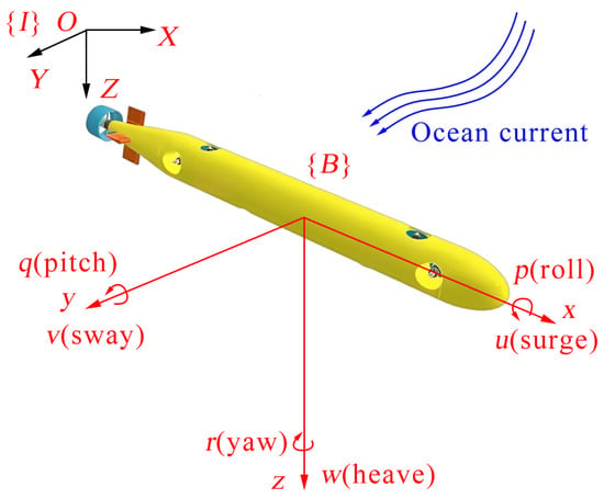
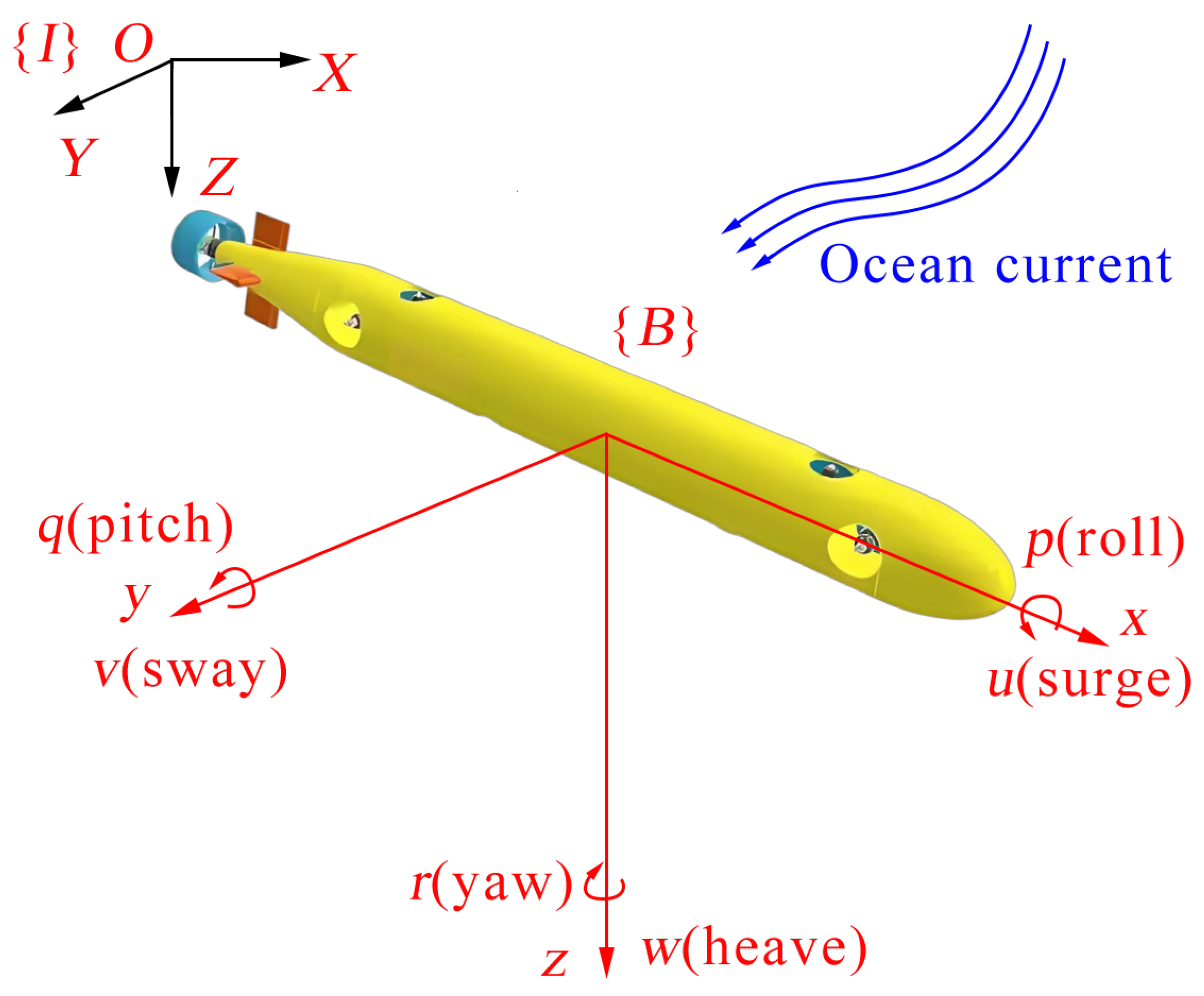
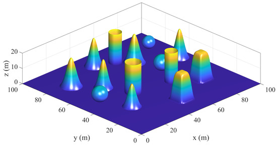
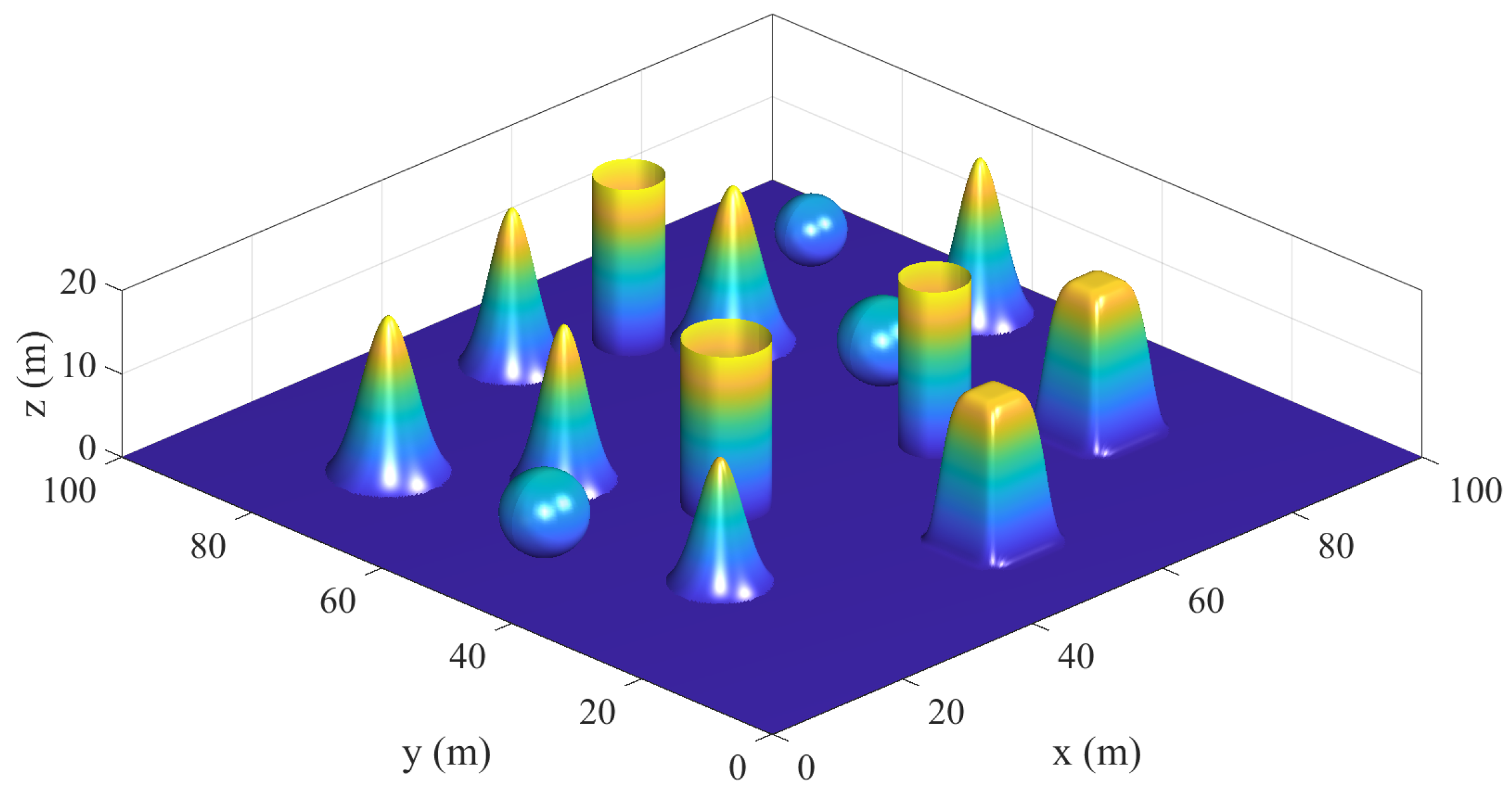
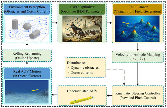
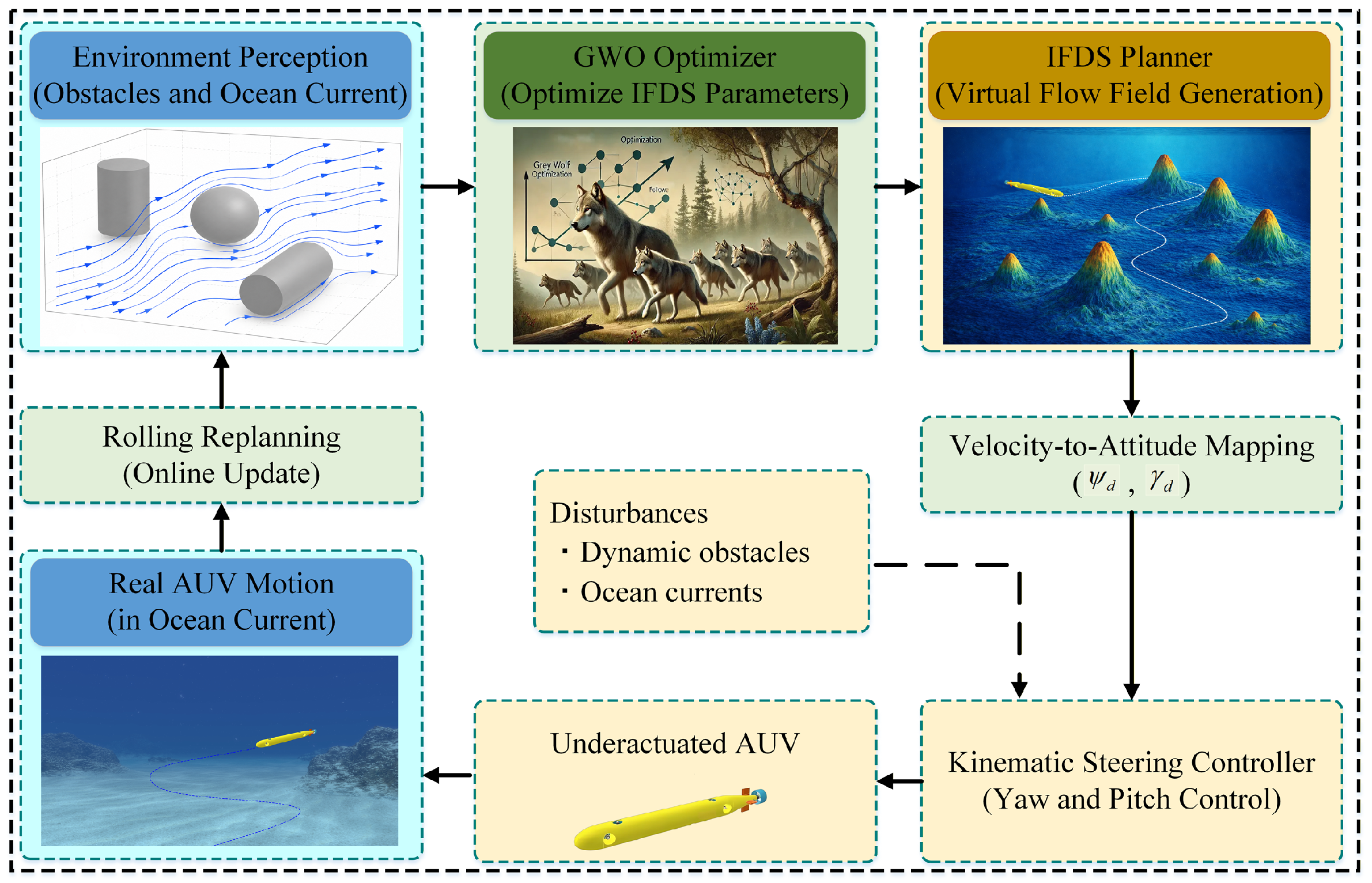
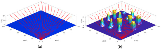
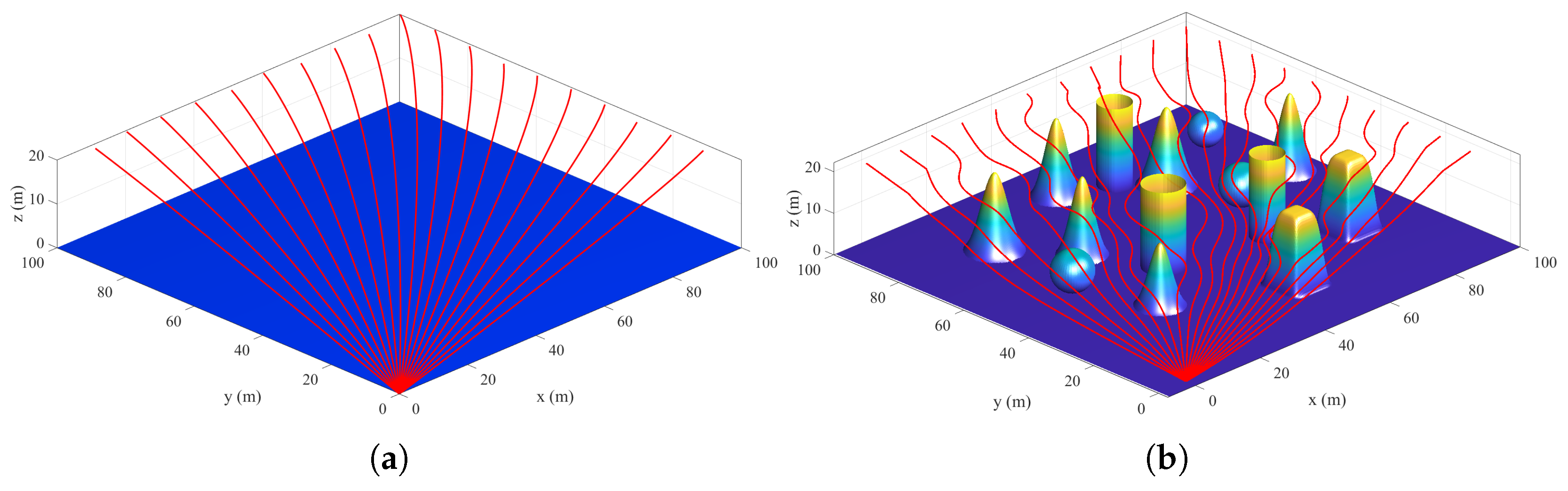
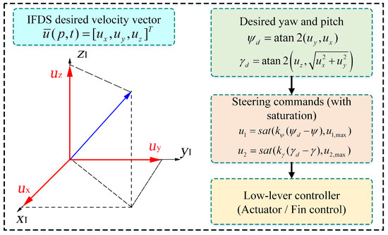
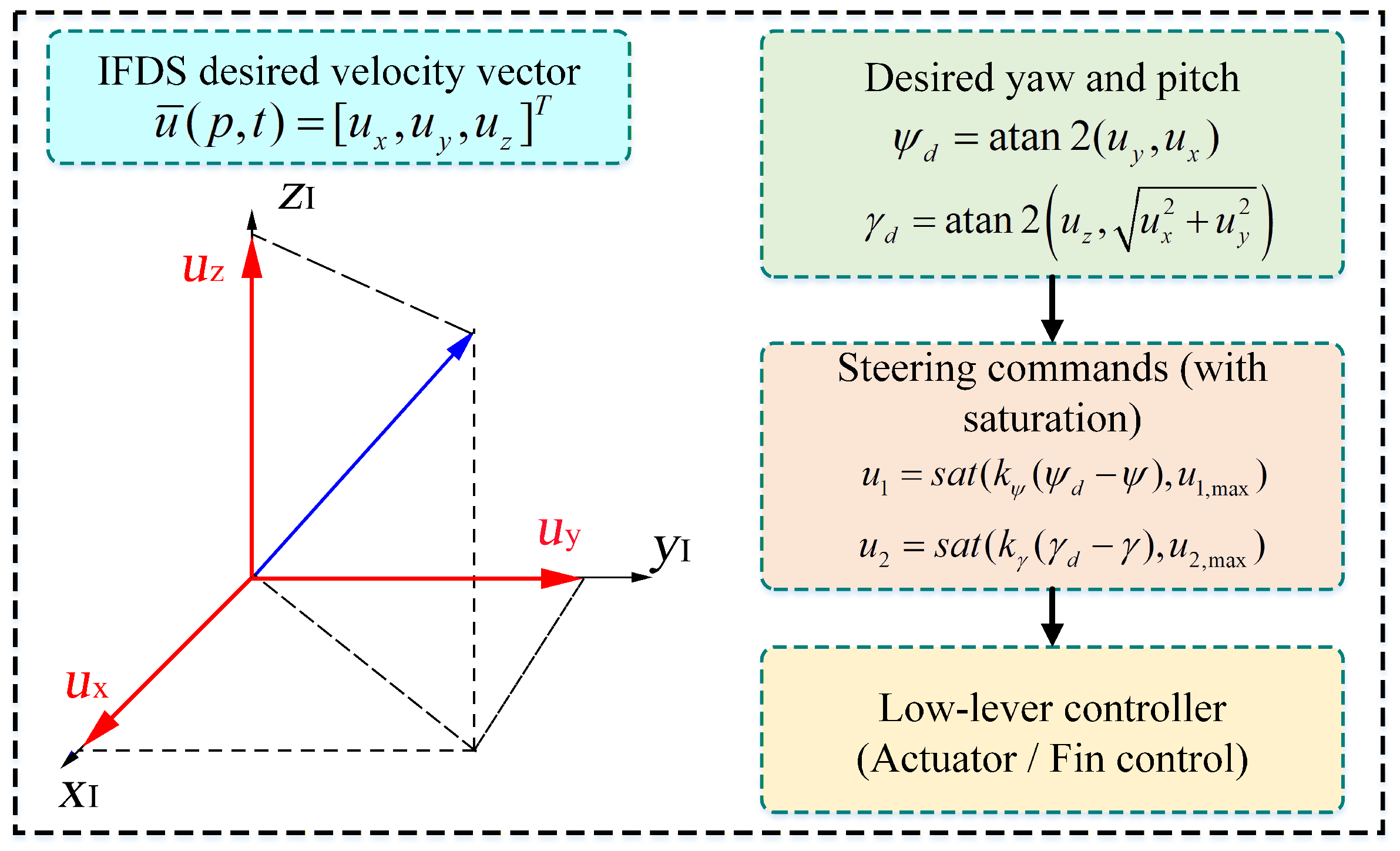
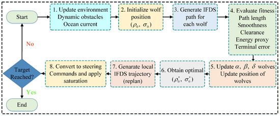
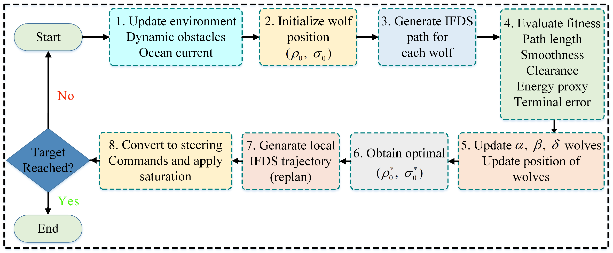
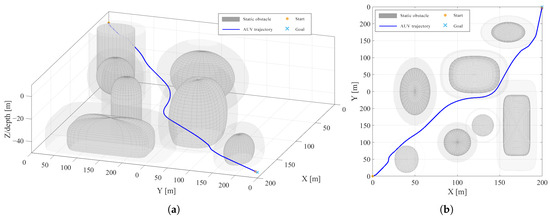
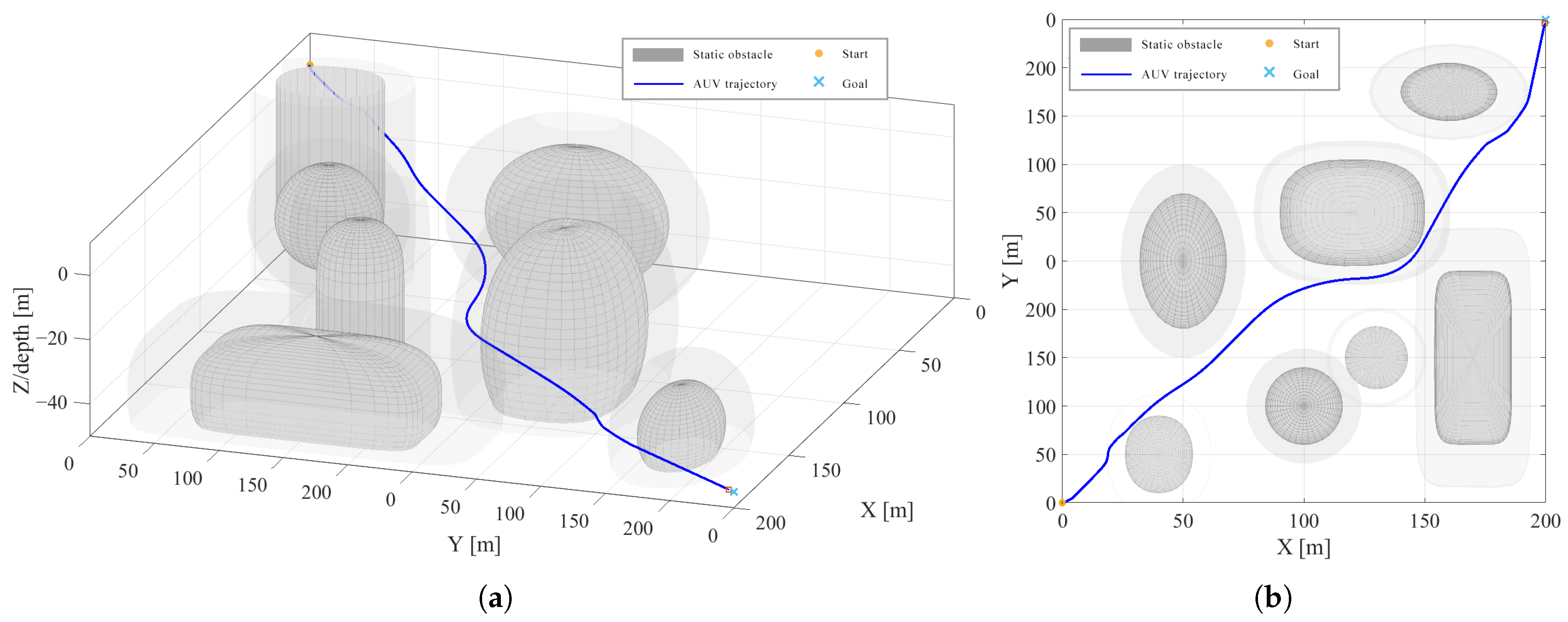
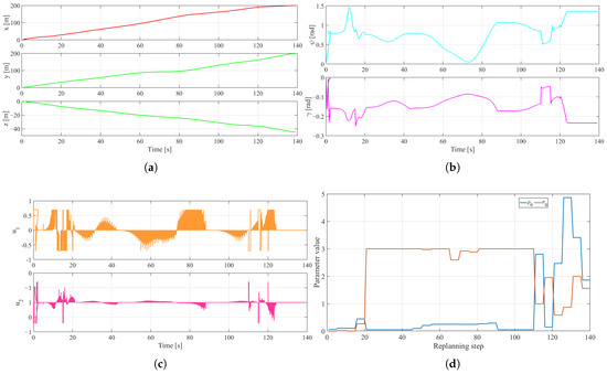
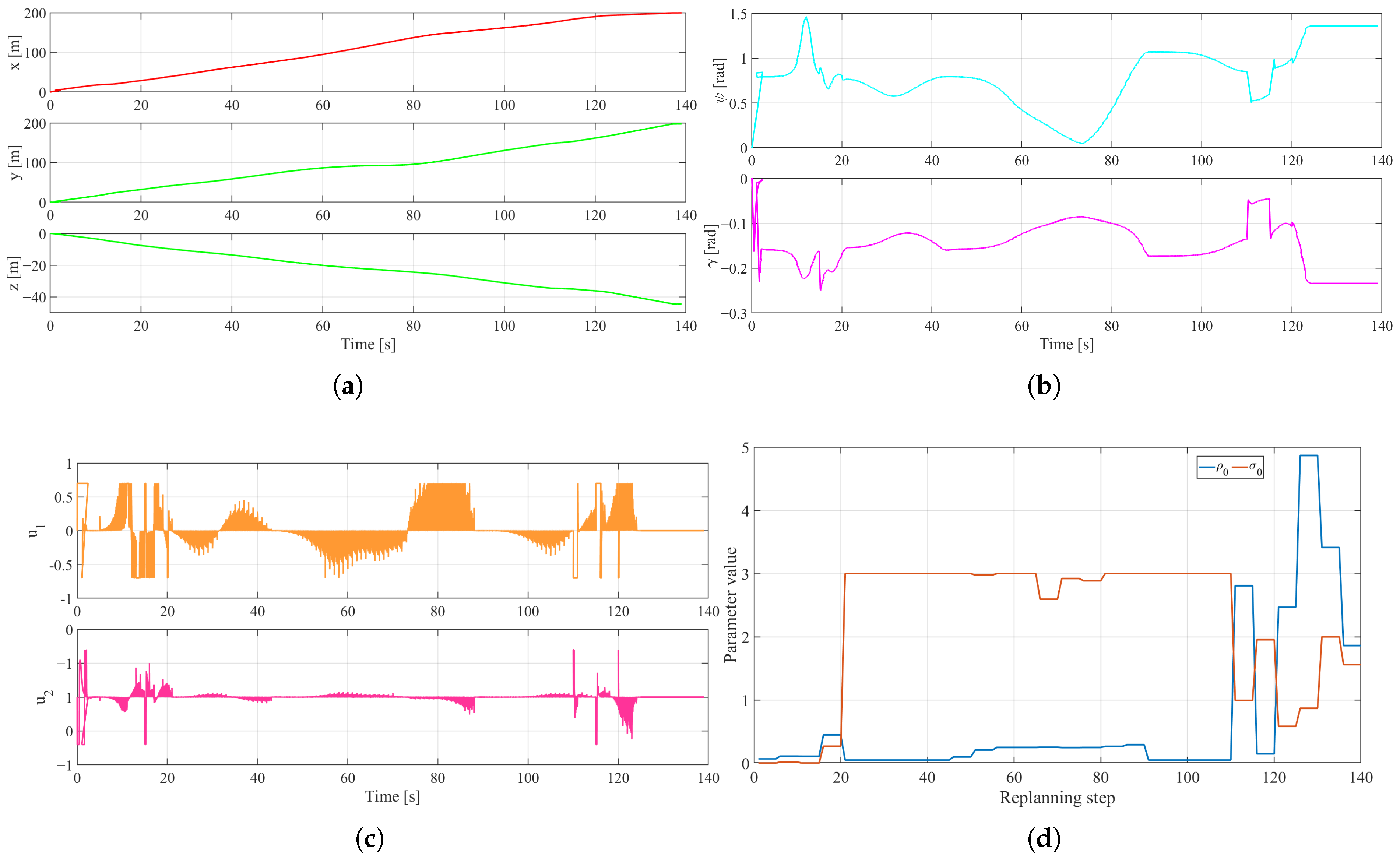
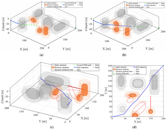
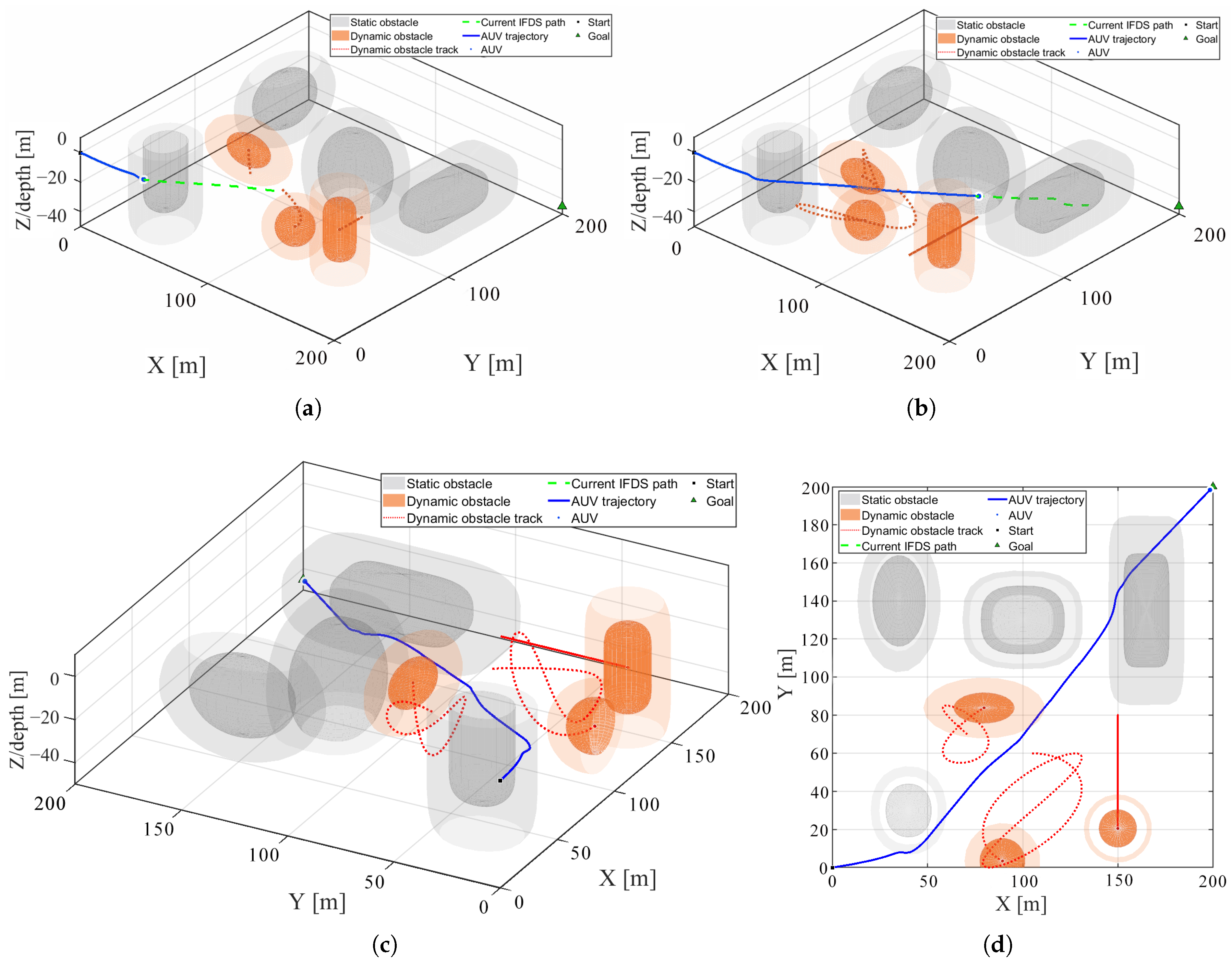
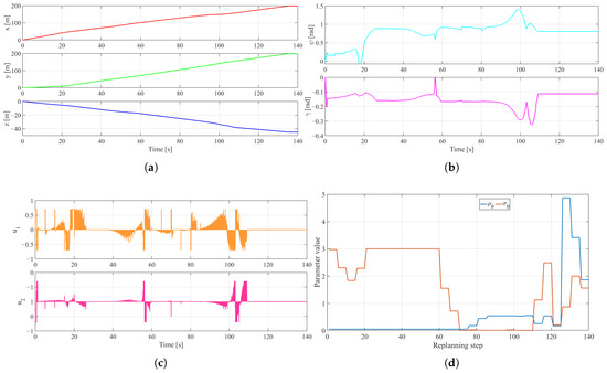
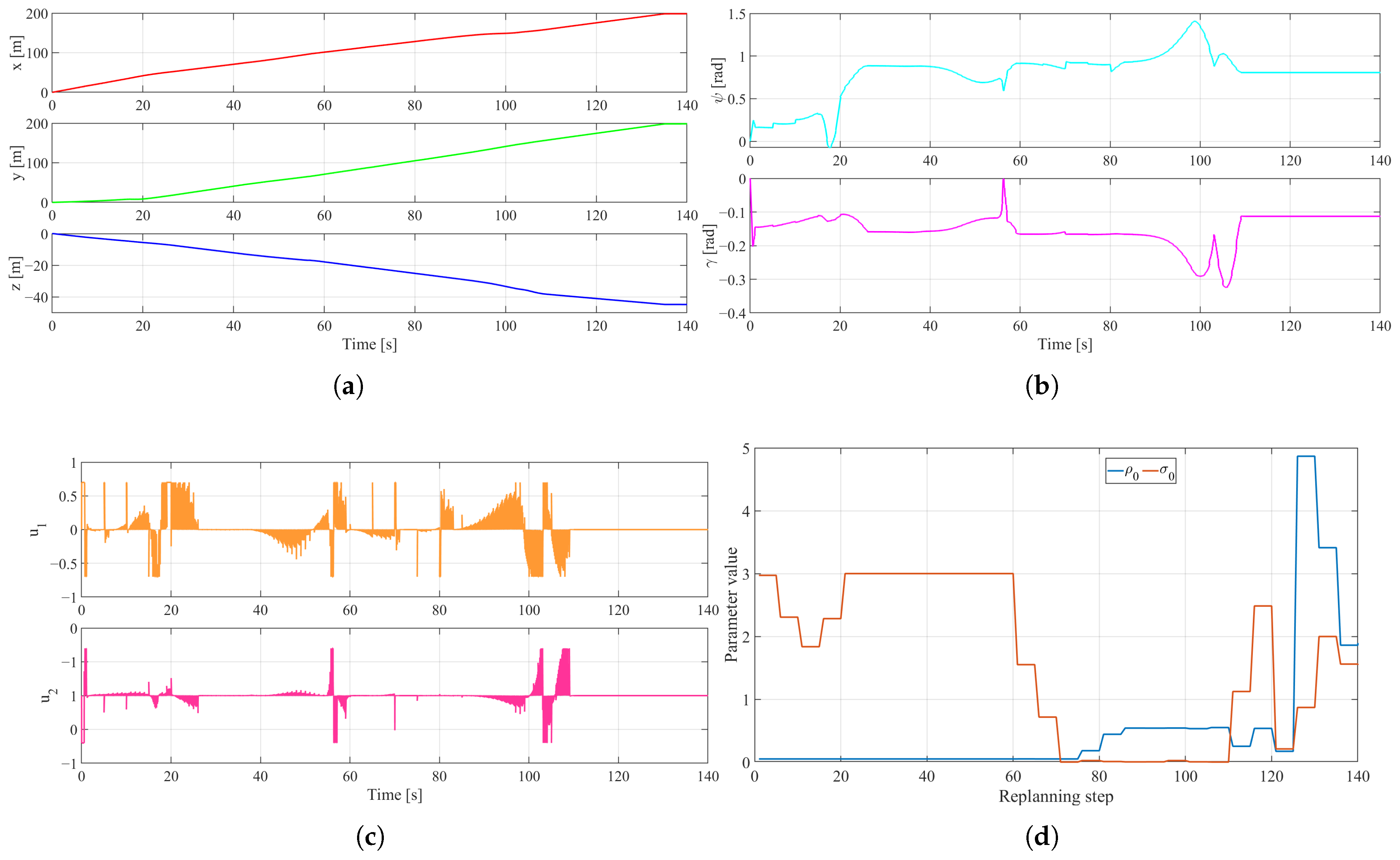
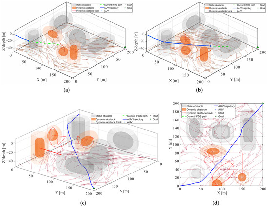
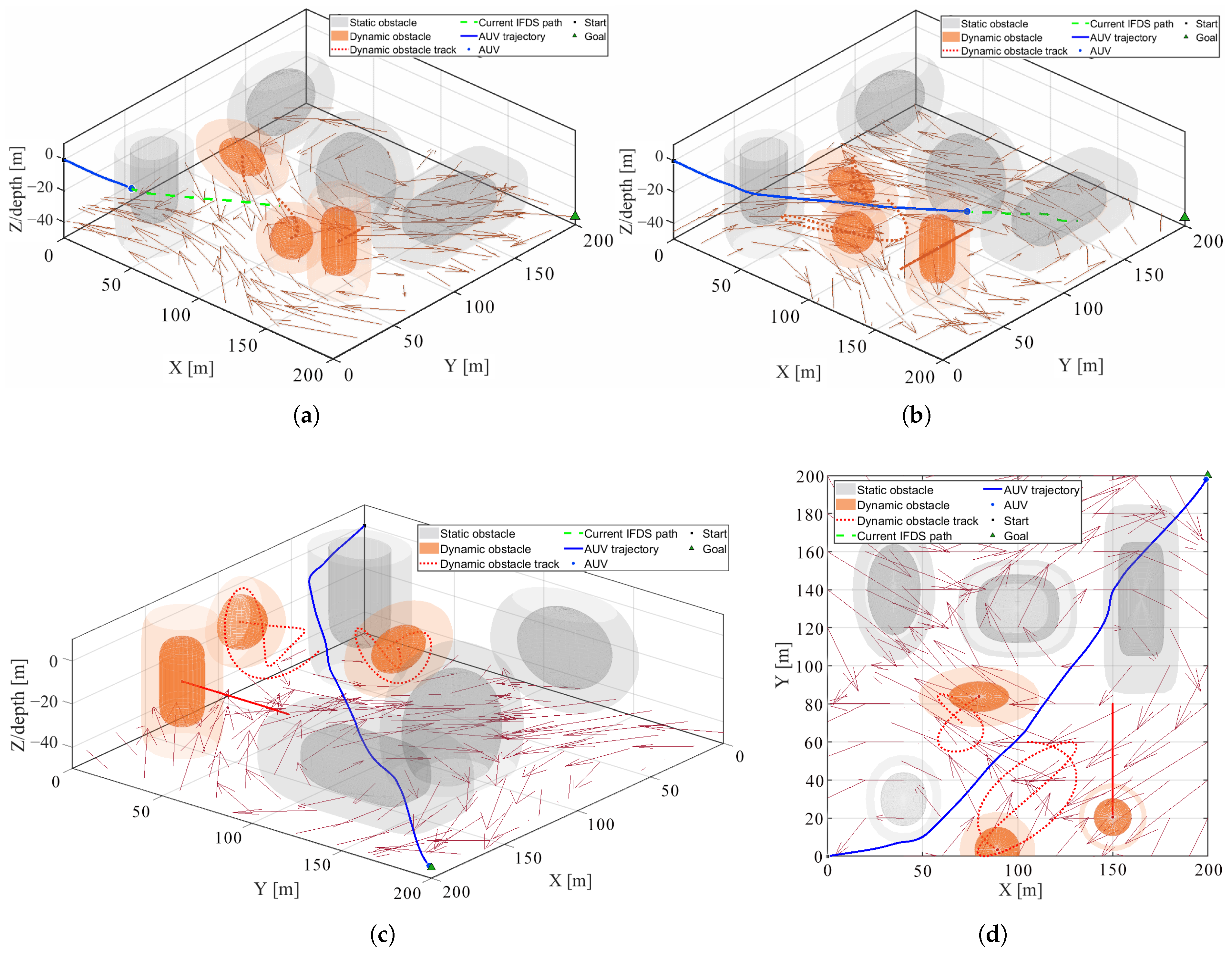
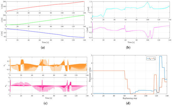
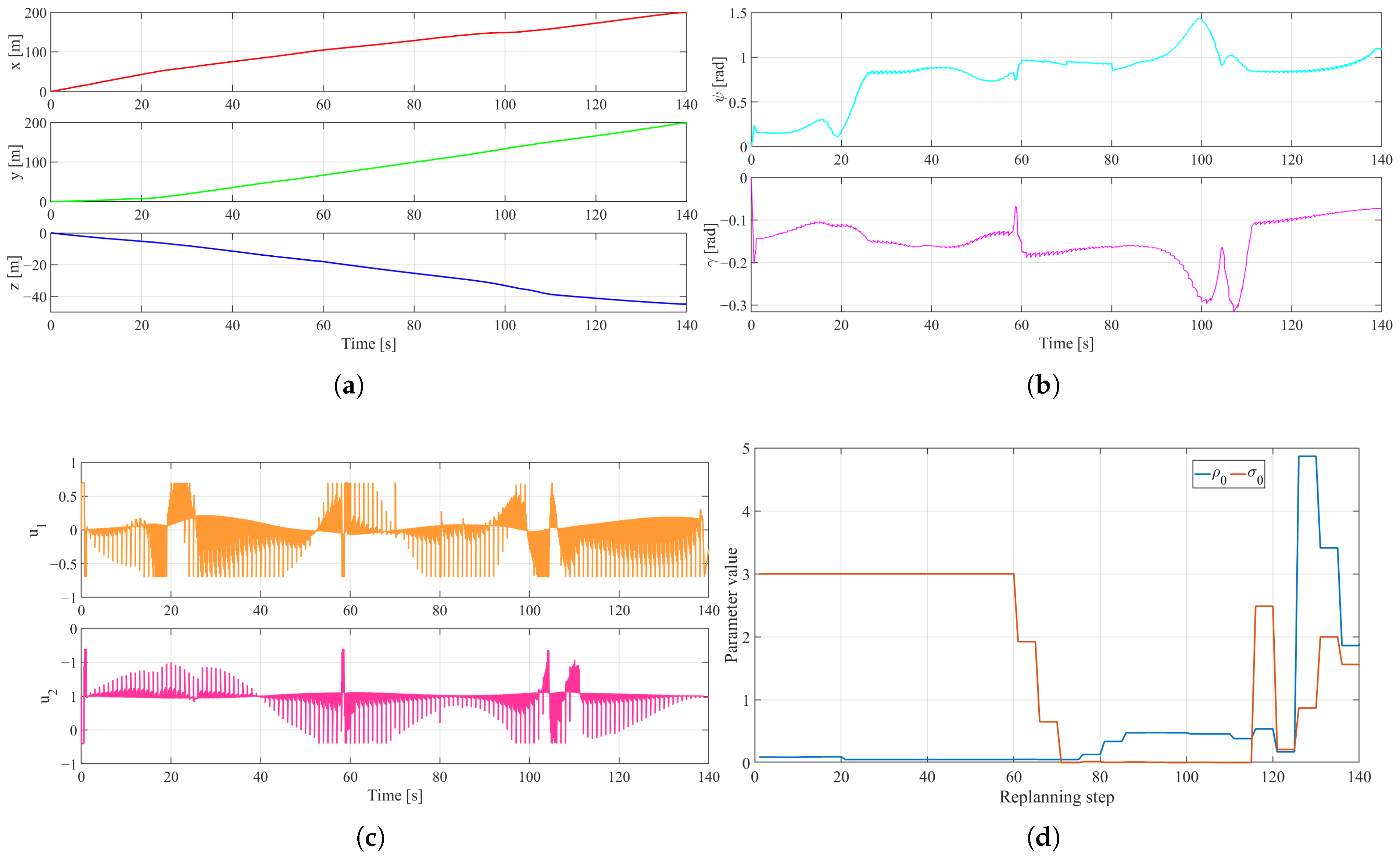
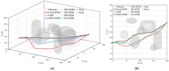
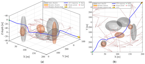
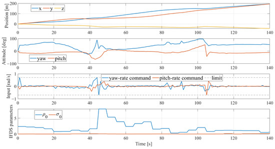

Disclaimer/Publisher’s Note: The statements, opinions and data contained in all publications are solely those of the individual author(s) and contributor(s) and not of MDPI and/or the editor(s). MDPI and/or the editor(s) disclaim responsibility for any injury to people or property resulting from any ideas, methods, instructions or products referred to in the content. |
© 2026 by the authors. Licensee MDPI, Basel, Switzerland. This article is an open access article distributed under the terms and conditions of the Creative Commons Attribution (CC BY) license.