


Highlights
What are the main findings?
- In consumer RGB drone imagery, submerged aquatic vegetation (SAV) appears as a local darkening of the water rather than as greenness: an excess-green index performs at chance, whereas local relative darkness separates SAV from open water with a cross-scene AUC of 0.969.
- Most SAV is smaller than the fixed lower limit on pixel number inherited from land-cover mapping. Pairing a ground-sampling-distance-anchored minimum mapping unit with a CFAR-inspired scale criterion recovers it, raising pixel recall from 0.52 to 0.71 with no false positives inside the annotated open-water rectangles.
What are the implications of the main findings?
- Low-cost, RGB-only drones can map where SAV is present and, within a stated spatial tolerance, how far it extends, including the small and fragmented stands that coarser sensors miss, with no multispectral hardware. The product is binary presence and extent only; it is not cover fraction, biomass, species identity, or a field-confirmed SAV map.
- The darkness and shadow limits of RGB remain physical and call for red-edge or near-infrared information, and low SAV prevalence bounds operational use. The spatial-scale limit, by contrast, is one that RGB can correct on its own.
Abstract
Submerged aquatic vegetation (SAV) is a sensitive indicator of shallow-water condition, but operational mapping has relied on multispectral, red-edge, or near-infrared sensing, leaving low-cost consumer RGB drones largely unused for the task. We present an RGB-only detector for SAV. It treats SAV as local darkening rather than a greenness signal, and sets the detectable patch scale with two label-free mechanisms, a ground-sample-distance (GSD)-anchored minimum mapping unit that rescales with altitude and a CFAR-inspired scale criterion N·(s/σ)2 ≥ τ driven by per-scene clutter σ. Across four densely annotated scenes most SAV is small, with 73–98% of labelled patches falling below the 0.43 m2 that a conventional fixed lower limit on pixel number retains at 4 cm GSD. Anchoring the minimum unit correctly raises pixel recall from 0.52 to 0.71 with no false positives inside the annotated open-water rectangles, and reaches a cross-scene SAV-versus-open-water AUC of 0.969, whereas an excess-green index performs near chance (AUC 0.438). Consumer RGB drones can therefore map binary SAV presence and extent within a darkness × scale detectability envelope, recovering the small, fragmented stands that coarser sensors miss, while cover fraction, biomass, species identity and the faintest SAV remain out of reach. The reference standard throughout is expert photointerpretation of 4 cm imagery, so what is mapped is image-interpreted SAV-like dark patches rather than field-confirmed SAV, and all results come from one lake system, one camera and one flight altitude.
1. Introduction
Submerged aquatic vegetation (SAV) is a structuring component of shallow freshwater and estuarine ecosystems. It stabilises sediments, cycles nutrients, oxygenates the water column, and provides habitat, and its presence and extent are widely used as integrative indicators of water-body condition [1,2]. Because SAV responds to eutrophication, hydrological alteration, and management intervention, its dynamics are a recurring target of monitoring [3,4,5,6]. Mapping SAV repeatedly over space and time nonetheless remains difficult, because the signal must be recovered through an attenuating water column [7].
Most operational SAV and aquatic-macrophyte mapping therefore relies on spectral information beyond visible light. Satellite multispectral and hyperspectral platforms, including Sentinel-2, PlanetScope, WorldView, and airborne hyperspectral sensors, are used to map macrophyte cover even in turbid and low-transparency waters [8,9,10,11,12,13]. These methods typically exploit red-edge and NIR contrast within bio-optical or geographic object-based models. The necessity of these bands is often explicit. Submerged canopies are detected by contrasting low in-water reflectance against the high NIR reflectance of near-surface or emergent material, and red-edge ranges have been compared directly against NIR for submerged targets [14]. Bio-optical approaches model the attenuation of light with depth to retrieve cover or biomass [15,16]. Dedicated indices have also been designed to remain invariant to depth or to extend the soil-line concept to variable water quality [17,18]. Reviews of satellite multispectral macrophyte mapping reflect this spectral dependence [19]. The approach has two clear limitations. Satellite pixel resolutions of 3 to 30 m miss small and fragmented stands, so low abundances go undetected [20], and even the best-case retrievals reported, obtained where the water column is clearest and the canopy densest, are confined to roughly 1.5 to 2.0 m depth in low-transparency water [8].
Unmanned aerial vehicles (UAVs) add centimetre-scale resolution to this toolkit. A substantial body of work maps aquatic vegetation from drones, predominantly with multispectral sensors and object-based image analysis (OBIA) [21,22,23,24,25,26], and increasingly for biomass and cover estimation by combining UAV and satellite data [27,28,29]. Consumer RGB drones, by contrast, are inexpensive, ubiquitous, and routinely flown by non-specialists, yet unfortunately they are often regarded as inadequate for SAV because they lack red-edge and NIR bands. Where RGB drones are used for aquatic primary producers, the targets are frequently floating or near-surface, such as green tides and filamentous or floating algae, for which a greenness contrast is valid [30,31,32]. Alternatively, RGB is paired with a multispectral sensor and its channels treated as auxiliary [33]. The few studies that apply RGB drones directly to submerged targets work in shallow, clear, non-turbid systems and treat the problem largely empirically [34,35]. Where RGB-only seasonal monitoring of submerged seagrass has been attempted, it was found insufficient to discriminate habitat change, and lowering the flight altitude did not help [36]. UAV multispectral imaging therefore reduces the resolution limitations of satellite data but keeps the spectral-band requirement and with it the sensor cost and calibration that limit consumer uptake. Consumer RGB is the one widely accessible alternative, yet what it can resolve for genuinely submerged vegetation in non-ideal water has not been established systematically.
This paper will look into two approaches that so far have not been attempted. Firstly, much RGB vegetation work transfers greenness indices designed for emergent or terrestrial canopies, such as excess green (ExG) and the normalised green–red difference. For SAV this is physically misplaced. A plant viewed through a water column does not present as “green” but as a local darkening of the water surface, because the column removes most of the upwelling pigment signal and what reaches the sensor is dominated by attenuation. The first aim of this paper is to make this explicit. We show that greenness is not merely weak but anti-informative for the SAV/open-water contrast, whereas local-relative darkness is a more suitable axis for detecting it.
Secondly, once a darkness-based detector is adopted, a subtle and, to our knowledge, untreated problem emerges: the size threshold applied to connected components. A “darker than surrounding water” rule highlights many small dark objects, only some of which are SAV. The remainder are sensor noise, ripple troughs, glint edges, shadow flecks, and floating debris. The standard remedy, inherited from land-cover mapping [37], is a minimum mapping unit (MMU): connected components smaller than a fixed pixel area are discarded. Such size thresholds are used in aquatic mapping too. For seagrass mapped from 3 m Planet satellite imagery, patches of at least about nine pixels, reported by those authors as ~200 m2, were almost always detected, and the same study used an occurrence-frequency threshold to suppress the isolated single-pixel misclassifications that appeared below that size [38]. Yet such thresholds are applied as fixed values, and their effect on recall is rarely quantified. The threshold buys precision at an unmeasured cost in recall, and it has two defects. It discards genuine small SAV patches that are, at the single-pixel level, spectrally indistinguishable from clutter, so the size threshold acts as a spatial proxy for a confidence the spectral data cannot supply. It is also expressed in pixels, so the same physical patch maps to a different pixel count at different altitudes and focal lengths, and a fixed lower limit expressed in pixels cannot transfer across acquisitions. This issue is not addressed even in careful UAV mapping-protocol guidance [39], and it matters wherever band choice and acquisition geometry are shown to change which vegetation is captured [40].
Four objectives follow. The first is to establish local-relative darkness, rather than greenness, as the RGB discriminative axis, and to build a transferable pixel detector on it. The second is to quantify how much genuine SAV a conventional fixed lower limit on pixel number discards. The third is to introduce two label-free mechanisms that recover it, a GSD-anchored physical minimum mapping unit and a CFAR-inspired scale criterion N·(s/σ)2 ≥ τ. The fourth is to delineate the resulting RGB capability boundary as a darkness-by-scale detectability envelope, and to test that boundary on deployment scenes acquired outside the calibration condition. Throughout, we respect a constraint stated by the survey operators: exhaustive annotation is too time-consuming to repeat, so any adaptive mechanism must be unsupervised at deployment.
2. Materials and Methods
2.1. Study Area and Image Acquisition
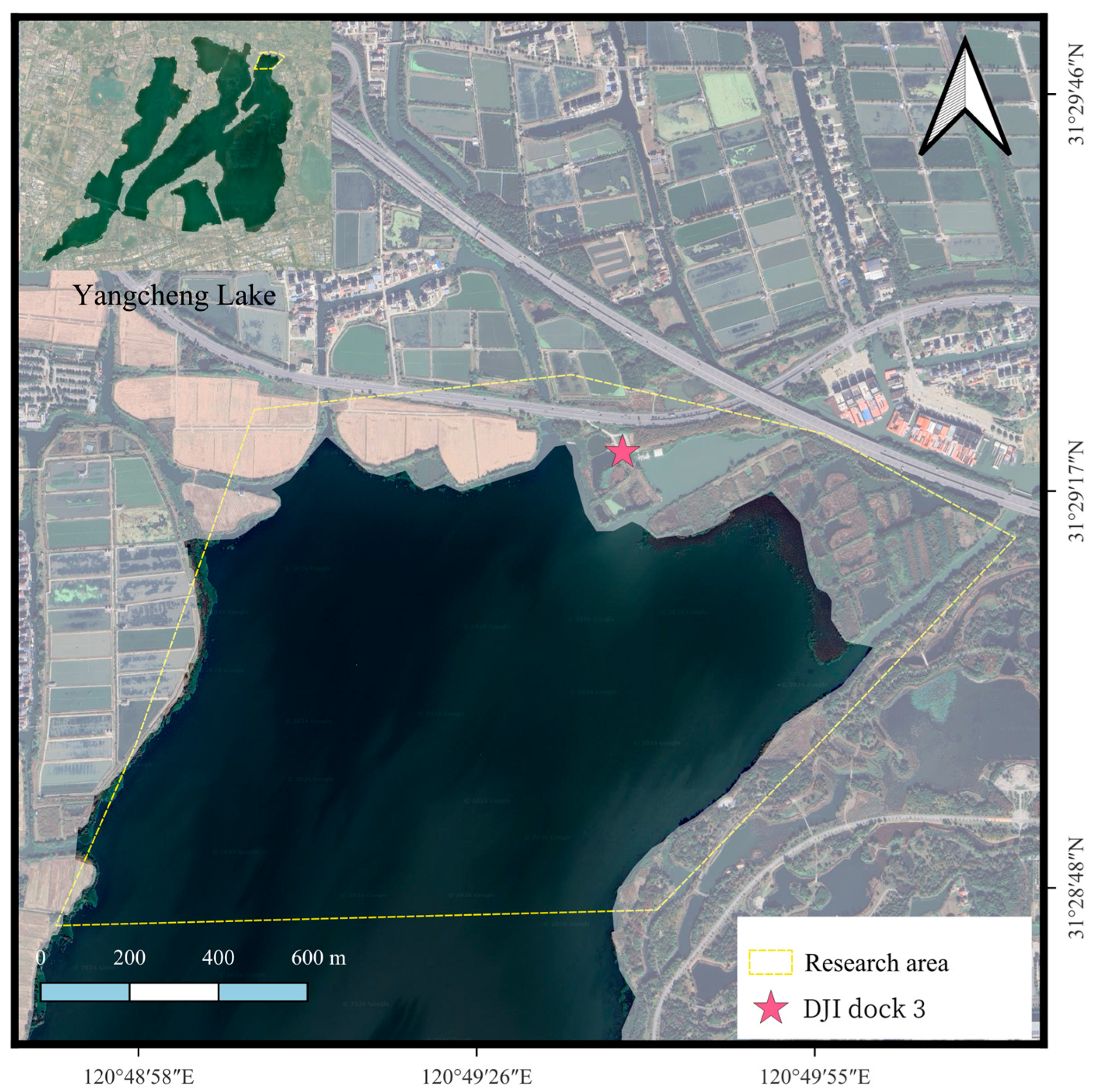
The study area is located in the north-east of Yangcheng Lake, Suzhou, Jiangsu Province, China (Figure 1), centred at 31.4847° N, 120.8248° E and spanning 31.4792° to 31.4903° N and 120.8140° to 120.8367° E. All positions are recorded in WGS 84, which is the coordinate system used by the flight-control system and the one in which the coordinates in Figure 1 are given. Because geographic coordinates are unsuitable for measuring area, the survey polygon and the flight track were projected to WGS 84/UTM zone 51 N (EPSG:32651) before measurement; in that projection the area covers 1.79 km2, over which a 13.6 km automated inspection route was planned and flown. Yangcheng Lake is a large, shallow freshwater lake in the Yangtze River Delta and a regionally important aquaculture water (particularly for Chinese mitten crab), where submerged aquatic vegetation strongly influences water clarity and habitat quality and is therefore a recurring monitoring target. An autonomous DJI Dock 3 (SZ DJI Technology Co., Ltd., Shenzhen, China) was deployed in the north of the area to support high-frequency, all-weather automated flights. Imagery was acquired with a DJI Matrice 4TD UAV (SZ DJI Technology Co., Ltd., Shenzhen, China; RGB camera, 4032 × 3024 px) at a relative flight altitude of approximately 111 m. This acquisition geometry yields a ground sampling distance (GSD) of 4.13 cm/px on the dense reference scene, computed from its recorded relative altitude of 110.95 m and 35 mm equivalent focal length of 24 mm (Equation (2)). Relative altitude across the annotated set varies between 109.7 and 115.0 m, so the GSD varies between 4.08 and 4.28 cm/px, a 4.8% variation within a single nominal flight altitude; we use 4.13 cm/px throughout because every derived patch-area quantity is computed on the dense scenes. Detection is performed at a working resolution of 1600 px on the long edge (10.4 cm/px), which bounds computation while remaining far finer than the SAV patch sizes of interest. Imagery was acquired mainly in the morning (~07:00–08:00) at near-nadir viewing geometry to suppress midday sun glint. Annotation was carried out in LabelMe (Version 6.2.0; open-source software, https://github.com/wkentaro/labelme, accessed on 25 July 2026), with SAV delineated as polygons and open water and the negative classes (wave, shadow, floating/emergent vegetation, land, etc.) as rectangles. Figure 2 summarises the full acquisition-to-detection workflow.
Figure 1.
Study area: A wetland in the north-east of Yangcheng Lake (Suzhou, Jiangsu, China). The dashed polygon marks the automated inspection extent (research area) and the star marks the DJI dock; the inset locates the site within Yangcheng Lake. Coordinates are shown in WGS 84; areas and route lengths were computed after projection to WGS 84/UTM zone 51 N (EPSG:32651).
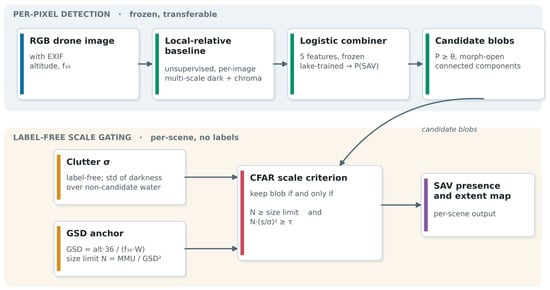
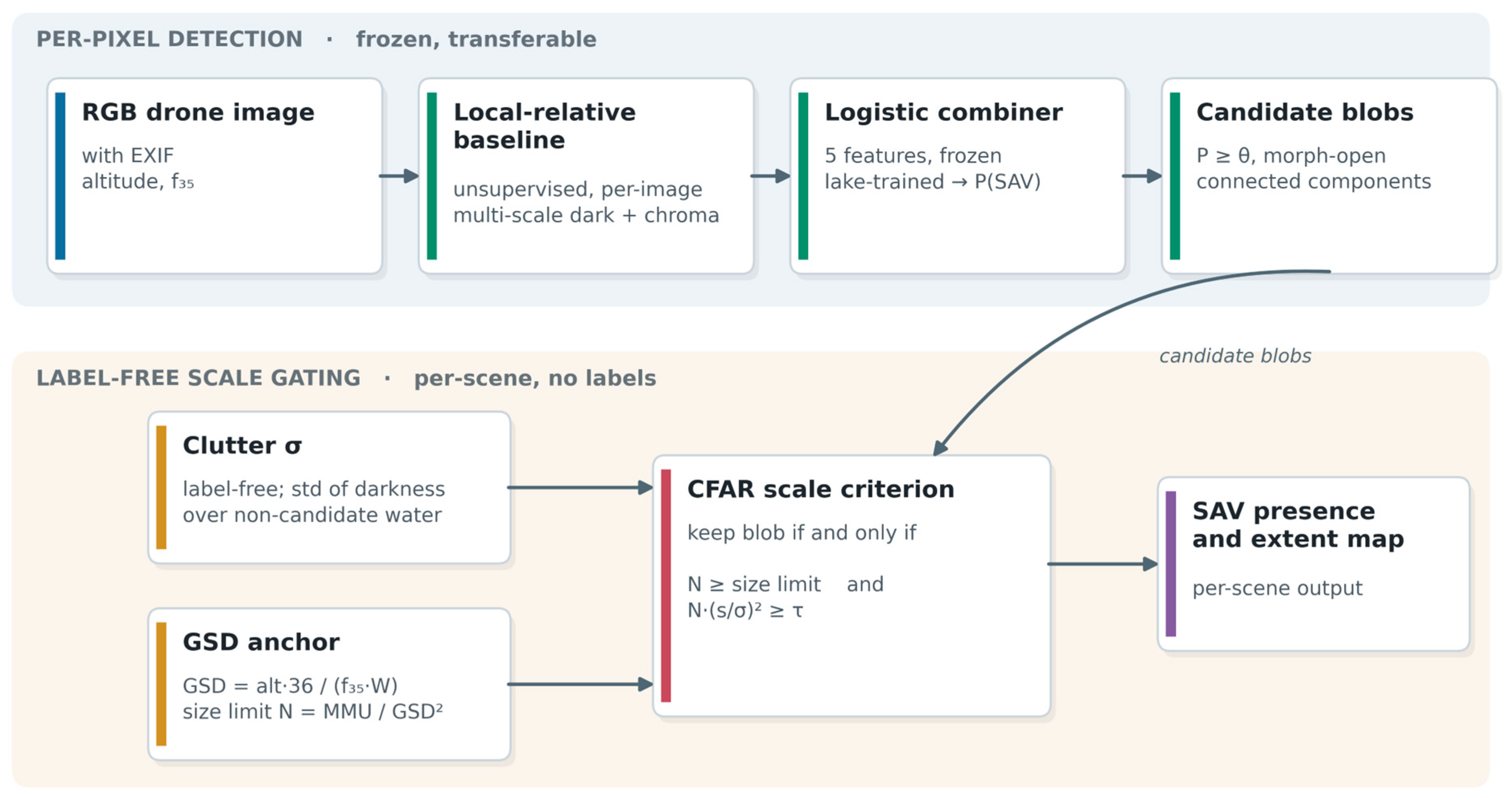
Figure 2.
Detector pipeline. Per-pixel local-relative detection (frozen, lake-trained, transferable) produces candidate blobs; label-free scale gating (per-scene clutter σ and a GSD-anchored size limit) then applies the CFAR scale criterion to yield the SAV presence/extent map.
2.2. Datasets and Annotation
Four datasets are used, with training and evaluation strictly separated. Throughout, the reference standard is expert photointerpretation of the 4 cm imagery rather than a synchronous in situ survey, so the target class consists of strictly image-interpreted SAV-like dark patches; when we refer to SAV below, this is what we mean. The combiner is trained only on the lake set, a separate collection of 17 densely binary-masked images (12 training/5 validation) representing the coherent-bed regime. Evaluation is performed on different scenes to test genuine cross-scene transfer, comprising the following: (i) a cross-scene box set of 58 frames spanning twelve acquisition dates across the monitoring season and a range of water levels and water-clarity (turbidity) conditions (a morning aquaculture-pond series plus several other dates and sites), annotated with SAV polygons and open-water rectangles (with floating/emergent vegetation labelled where present), totalling 1197 SAV and 512 open-water shapes, used for box-level discriminability. Two further box-annotated frames exist but are excluded from all evaluation: on checking the datasets against each other we found them to be pixel-identical to two of the twelve lake images on which the combiner was fitted, so retaining them would have placed training scenes inside the cross-scene test. Excluding them raises the cross-scene AUC of the proposed detector from 0.967 to 0.969, so the exclusion is conservative in direction as well as correct in principle; (ii) four dense scenes in which every SAV patch is exhaustively labelled (one full frame of 1391 patches plus three native-resolution crops), used as the measuring stick for the scale analysis (exhaustive whole-frame annotation is prohibitively slow, so dense labelling is confined to these reference scenes); and (iii) a deployment set of three unlabelled images (same-condition open water, diffuse green water, midday glint), used to test robustness against flooding under changing conditions.
2.3. Local-Relative Pixel Detector
The water column renders absolute radiometric quantities unreliable: white balance, sun angle, and water colour vary between and within scenes, so a detector keyed on absolute brightness or a single global threshold saturates when conditions change. We therefore use only local-relative features, all computed in CIELAB (luminance , chroma components , ) and HSV (hue, also used to exclude glint). Each image is first resized to a working resolution of 1600 px on the long edge; a smooth open-water baseline luminance field is then estimated by an unsupervised background-estimation procedure analogous to astronomical source extraction (SExtractor) [41]: on three grid scales (32, 96, 256 px at working resolution) the bright-side 75th percentile within each cell serves as the open-water reference, iterated three times (excluding pixels with before re-estimation) and interpolated back to full resolution by bicubic interpolation. The per-pixel features are three-scale dark residuals (where is the local baseline luminance at each scale, the pixel luminance, and a local robust scale), together with the local chroma deviation and hue deviation relative to the surrounding water, giving five features in total (dark residuals clipped to , chroma and hue to ). Absolute brightness and any global normalisation are deliberately excluded.
The five features are combined by a single low-capacity linear (logistic) rule. Because the features are physically motivated (submergence darkens the water and only weakly shifts its colour relative to the surrounding open water), the combination needs no high-capacity learning: its five coefficients and a bias are calibrated once, by a logistic fit on an independent set of densely masked images from the same lake system, and then frozen and applied unchanged to every scene reported here. The calibration is strongly over-determined (of order 4 × 10⁵ labelled water pixels constraining six parameters), and, because the frozen rule is never refitted per image, the cross-scene results reflect genuine transfer rather than per-scene tuning. Crucially, the calibration confirms the mechanism rather than discovering it: the three dark-residual terms dominate (small/mid/large-scale coefficients of 0.19/0.44/0.36), chroma is secondary (0.20), the hue (greenness) term is effectively null (−0.06), and the bias is −2.06. That is, darkness, not colour, carries the signal, exactly as the radiative-transfer argument predicts. The feature standardisation statistics are stored with the coefficients, so the frozen rule reproduces deterministically. The water mask additionally excludes land and emergent vegetation (high ExG > 25 together with high local texture, std , dilated by a 14 px shoreline buffer to remove shaded water hugging tree-lined banks that would otherwise read as false SAV) and residual specular glint ( and ), followed by a 5 × 5 morphological opening; these gates are used only to build the analysis mask and are never fed as features. The output is a continuous per-pixel SAV probability within the water area.
2.4. CFAR-Inspired Scale Criterion
Candidate pixels are those whose SAV probability exceeds a threshold (, a deliberately permissive high-recall inclusion threshold whose only role is to admit components for the subsequent scale test, so the discriminative decision is governed by rather than by ); after a 3 × 3 morphological opening to remove speckle, they are grouped into connected components under 8-connectivity. For each component we record its area (pixels) and its mean darkness contrast (the mean of over the component, with the mid-scale local baseline). We treat detection against a clutter background as a matched-filter, or constant-false-alarm-rate (CFAR), problem [42]. The statistic follows from incoherent integration over the component: for a region of pixels, each carrying a mean darkness contrast against benign-water clutter of standard deviation , the integrated signal grows as while the integrated clutter (summing approximately independent fluctuations) grows only as , so the squared detection signal-to-noise of the whole component is
The single-pixel contrast test () is the special case, and area integration is what lets a faint but extended patch clear the threshold that an individual pixel cannot. A component is retained if and only if the following conditions apply:
The clutter level is estimated per scene and without labels as the standard deviation of the darkness field over non-candidate water (probability below θ_cand), i.e., the natural fluctuation of benign water ( on the dense scenes here). The threshold is the single exposed operating point (default , chosen from the recall–precision trade-off); it is the detection threshold on the integrated statistic and can be bound to an external constraint such as measured transparency (Secchi depth or ), with larger being stricter. The area lower limit is provided by the physical anchor of Section 2.5 (degrading to an absolute lower limit of 4 px when metadata are absent). In the plane this criterion is a hyperbola, in contrast to the vertical line of a hard size threshold. The formulation extends the one-dimensional “per-pixel contrast against noise” detectability condition to the two-dimensional (contrast × area) plane. We call the criterion CFAR-inspired rather than CFAR because it is not a calibrated constant-false-alarm-rate detector in the classical sense: τ is chosen empirically from the recall–precision trade-off rather than derived from a nominal false-alarm probability, the clutter distribution is not modelled explicitly, and the approximate independence of neighbouring pixels assumed by the incoherent-integration step is not tested. The statistic is therefore best read as a matched-filter-like scale criterion whose operating point is set empirically, and the achieved false-alarm rate is an empirical quantity that varies between scenes rather than a constant guaranteed by construction.
2.5. GSD-Anchored Minimum Mapping Unit
To make transferable across scenes, we anchor it to a physical minimum mapping unit (MMU, m2) rather than a fixed pixel count. Under a pinhole-camera projection at near-nadir viewing, the ground footprint width imaged by the sensor is , where and are the physical sensor width and focal length. The 35 mm equivalent focal length reported in EXIF is defined so that , which removes any dependence on the actual sensor size. Dividing the footprint by the image width in pixels gives the per-pixel ground size, so from only two EXIF fields, the relative altitude alt (RelativeAltitude) and the 35 mm equivalent focal length f35 (FocalLengthIn35mmFormat), the working-resolution GSD is:
where 36 mm is the full-frame reference width and the working-resolution image width in pixels. Because the physical sensor width cancels, the anchor requires no camera-specific calibration and is, in principle, portable across platforms from metadata alone; this portability is established analytically here and is not validated empirically: all imagery in this study comes from one camera at one nominal altitude, so the cross-altitude and cross-camera behaviour of the anchor remains untested. The pixel-number lower limit is then set to . The same physical MMU maps to more pixels at lower altitude and fewer at higher altitude, so the criterion rescales automatically with acquisition altitude and camera. For the present data, the M4TD with alt = 110.95 m, f35 = 24 mm and = 1600 gives = 10.4 cm/px; a default MMU = 0.08 m2 (≈ 29 cm clump, the 25th percentile of labelled SAV patch sizes) corresponds to px. When metadata are absent, the procedure degrades to an absolute lower limit of 4 px.
2.6. Baselines and Evaluation
We compare the results against three baselines representing standard practice, all scored against the same dense ground truth within the same water mask. The greenness baseline is an ExG (excess green, ) threshold within water (>10), representing the “find green vegetation” approach inherited from terrestrial and floating-vegetation work [30,31]. The global-darkness baseline is a global Otsu threshold on within-water luminance, representing the naive “SAV = dark water” rule. The fixed-MMU baseline is the local-relative detector (candidates with probability ≥ 0.28) followed by a fixed 40 px MMU, representing the conventional connected-component minimum-mapping-unit approach. Our method is the CFAR criterion with the GSD anchor.
Pixel-level recall, precision, and F1 are computed on the dense reference scenes and the lake validation masks. Each image estimates its own baseline (no global fit); the logistic combiner is fitted on 12 lake images and then frozen and transferred to all cross-scene data (the lake set is split 12 training/5 validation). Cross-scene discriminability is reported as the box-level SAV-versus-open-water AUC over the 58-frame set (1197 SAV and 512 open-water shapes), from which the two frames identical to training images have been removed: each annotated shape is scored by its internal predicted-SAV pixel fraction, and the AUC is the rank-sum (Mann–Whitney U) statistic. We additionally report per-negative-class predicted coverage as a false-positive indicator, and whole-frame coverage on the deployment images. Because the dense ground truth uses tight polygons whereas detections are slightly dilated, precision is reported at zero tolerance and within ±2/±3 px tolerance to distinguish true false positives from boundary halos. The tolerance is defined at the working resolution, so ±2 px corresponds to about 21 cm and ±3 px to about 31 cm on the ground; all extent statements in this paper are bounded by that tolerance. Object-level metrics count an annotated patch as recovered when it intersects a predicted component, with IoU ≥ 0.5 reported additionally, and 95% confidence intervals are obtained by bootstrap resampling of patches (1000 resamples). All processing is implemented in Python (Version 3.10.20) with OpenCV (Version 4.13.0), NumPy (Version 2.2.6), SciPy (Version 1.15.3) and scikit-learn (Version 1.7.2, logistic regression); acquisition metadata are read with ExifTool (Version 13.56).
3. Results
The results are organised along the axes of the identifiability argument. Section 3.1 establishes the discriminative axis by contrasting greenness with local-relative darkness. Section 3.2, Section 3.3 and Section 3.4 address the scale axis: how the detectors compare, how much SAV a fixed lower limit on pixel number discards, and how anchoring that limit to the ground sampling distance makes it transferable in principle. Section 3.5 and Section 3.6 characterise the CFAR-inspired criterion and its single operating point. Section 3.7 then applies the detector to deployment scenes acquired outside the calibration condition and reports a point-based validation of what it maps there.
3.1. Greenness Versus Local-Relative Darkness
The excess-green (ExG) index separates SAV from open water at an AUC of only 0.438 (Table 1), which is essentially a matter of chance and indicates that greenness carries almost no usable SAV-versus-open-water signal. This is consistent with the physical expectation that pigment colour is attenuated through the water column while the dominant effect is darkening. A global-darkness threshold is better but still weak (Table 1) and saturates at the pixel level (F1 ≤ 0.05), because a single global cut cannot accommodate the within-scene baseline variation in water colour and illumination. Only the local-relative formulation resolves this. This result directly motivates abandoning greenness indices for submerged targets, in contrast to their valid use for floating and emergent vegetation.
Table 1.
Detector comparison. Pixel recall/precision/F1 on the dense reference scene and the lake validation masks; cross-scene SAV-versus-open-water box AUC (higher is better).
3.2. Baseline Comparison
Table 1 reports all four detectors under the same ground truth and metrics; the cross-scene AUC is computed over the 58 box-annotated frames (1197 SAV and 512 open-water shapes) spanning twelve dates and a range of water levels and clarity, so it measures discriminability across temporal and hydrological variation rather than within a single condition. The naive greenness and global-darkness baselines fail (pixel F1 0.04–0.05; cross-scene AUC 0.438 and 0.803). The two local-relative detectors are both strong discriminators at the box level: the fixed-MMU detector reaches AUC 0.950 and CFAR 0.969. The box-level AUC, however, is insensitive to the recall of small patches, because a shape is scored by its internal predicted-SAV fraction and a few large detections already light it up. CFAR’s distinctive advantage is therefore not visible here but in the dense pixel-level recall of small patches, where it leads on F1 (dense image 0.395 vs. 0.354; lake 0.376 vs. 0.361). The same ordering holds at the object level on the full-frame reference scene, where CFAR reaches a patch recall of 0.577 (95% CI 0.542–0.615) and a patch precision of 0.788 (0.759–0.817) against 0.260 (0.233–0.287) and 0.928 (0.897–0.956) for the fixed 40 px baseline and leads on patch recall at every matching threshold tested, including IoU ≥ 0.5 (0.136 vs. 0.085).
Dense F1 is the pixel-level metric on the full-frame dense reference scene; Lake F1 is the pixel-level metric on the lake validation masks; cross-scene AUC is the box-level SAV-versus-open-water metric over the 58 box-annotated frames. The box-level AUC separates the fixed-MMU and CFAR detectors only slightly because it is insensitive to small-patch recall; the size effect appears at the pixel level (Table 2).
Table 2.
Size operating point on the dense reference scene (pixel metrics vs. dense ground truth). None of the three configurations placed a single predicted SAV pixel inside the annotated open-water rectangles: 0 of 9829 pixels in every case, a 95% upper bound of 0.03% on the commission rate within those declared negatives.
3.3. The Size-Limit Recall Loss
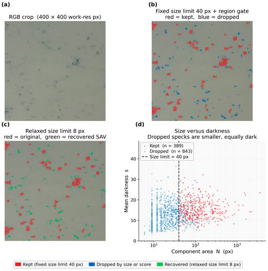
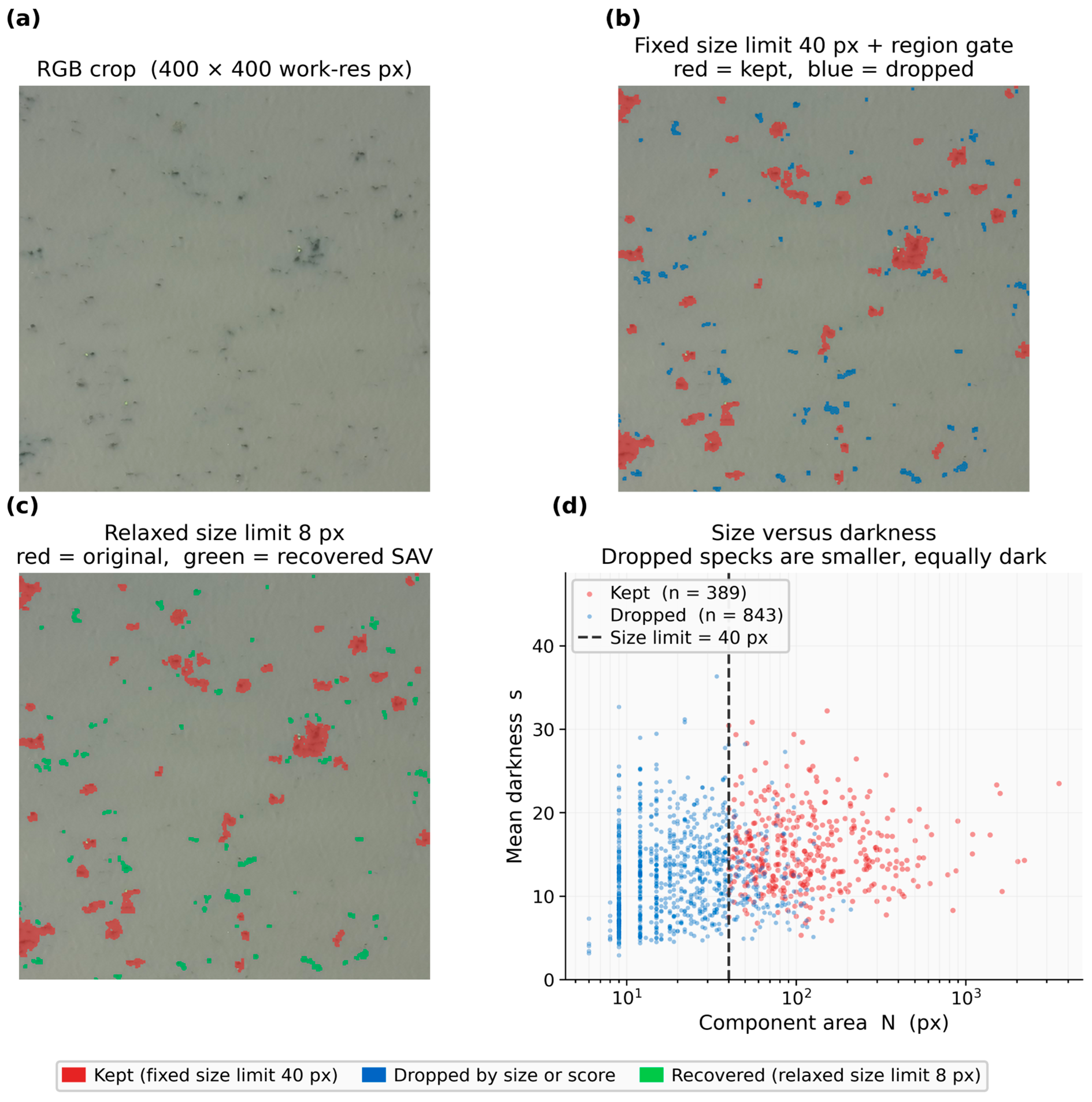
Using the dense reference scene, we swept the size operating point and decomposed the recall loss by patch size (Figure 3; Table 2). Removing the hard threshold raised pixel recall from 0.519 to 0.708, a gain of 19 percentage points (37% relative), with per-pixel precision essentially unchanged (0.258 → 0.267) and no false positives inside the annotated open-water rectangles throughout. This last quantity is measured only within the annotated open-water rectangles and the selected negative classes, not over all non-SAV water, so it bounds commission inside declared negatives rather than establishing a zero false-alarm rate. The lost SAV is not at a physical limit: across all size bins, 0% of labelled patches vanish at working resolution and 0% fall below the candidate darkness threshold. The patches are dark enough and resolved enough to become candidates; they are removed purely by the size proxy. Detection rate rises monotonically with both patch size and threshold relaxation; for example, the 30–80 px bin rises from 0.33 to 0.70.
Figure 3.
Most SAV is small and recoverable (a native-resolution crop of the dense reference scene). (a) RGB crop. (b) Connected components kept (red) vs. discarded (blue) by the fixed 40 px lower limit on pixel number. (c) Small SAV specks recovered (green) when the size limit is set correctly. (d) Component size vs. darkness: the discarded specks are smaller but equally dark.
This is not specific to a single scene. Across four exhaustively annotated scenes (the full-frame reference and three native-resolution crops), real SAV patches are consistently small relative to the fixed mapping unit (Table 3). Median patch areas range from 0.08 to 0.27 m2, and 73–98% of all labelled patches fall below the 0.43 m2 implied by the fixed 40 px threshold (median across scenes ≈ 90%). Because patch area is a property of the vegetation and the GSD rather than of the detector, this statistic is independent of the processing resolution and confirms that a fixed pixel threshold discards most real SAV across scenes.
Table 3.
Real SAV patch sizes across the four exhaustively annotated scenes (GSD 4.13 cm/full-px). The fixed 40 px threshold implies a 0.43 m2 minimum mapping unit on a full frame; most labelled patches fall below it.
Per-pixel precision against the tight polygons is 0.27 at zero tolerance but rises to 0.57 and 0.68 within a 2- and 3-pixel tolerance, respectively. Most of the apparent false positives are therefore boundary halos around the tight polygons rather than spurious detections. The remainder reflects a mixture of genuine false positives and SAV still missing even from the dense annotation (predicted coverage 5.0% vs. annotated 1.9%). Precision is thus best read as an interval. Per pixel, the size sweep does not degrade it; at the object level the same relaxation trades 27 points of patch precision (0.928 → 0.659) for more than a doubling of patch recall (0.260 → 0.582).
This effect is regime-dependent. On the lake set, where SAV forms coherent beds rather than sparse specks, relaxing the threshold adds little recall (+0.03) at a small precision cost (F1 flat to slightly negative). The harm of a fixed threshold therefore scales with how fragmented the SAV signal is, i.e., with growth form and GSD, so a single fixed value is systematically wrong across scenes.
3.4. GSD Anchoring of the Size Limit
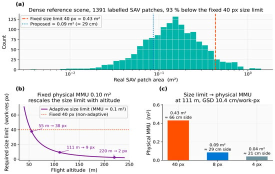
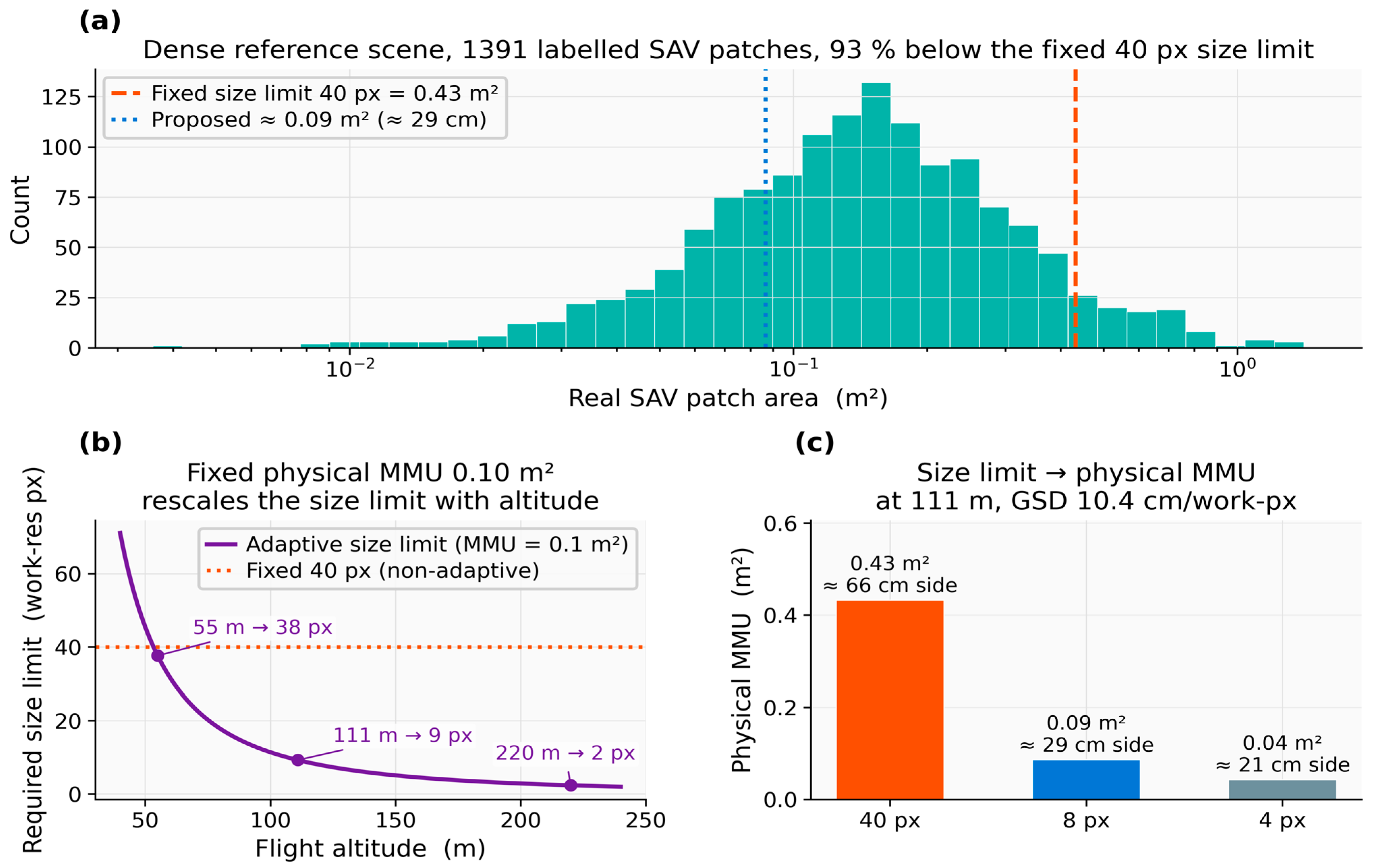
At 111 m altitude the GSD is 4.13 cm/px (10.4 cm/px at working resolution; 108 cm2 per working pixel). The current 40 px threshold therefore corresponds to a 0.43 m2 minimum mapping unit, i.e., a 66 cm clump (Figure 4). By contrast, the labelled SAV patches on the full-frame reference scene have a median area of 0.14 m2 (38 cm) and a 25th percentile of 0.086 m2 (29 cm). Thus 93% of patches are smaller than the 40 px MMU and are removed by size alone, and this holds across the four densely annotated scenes (73–98% below the MMU; Table 3). The empirically good threshold (8 px ≈ 0.087 m2) coincides with the 25th percentile of real patch sizes, i.e., a physically reasonable minimum clump.
Figure 4.
GSD-anchored physical minimum mapping unit. (a) Distribution of real SAV patch area on the dense reference scene, with the 0.43 m2 unit implied by the fixed 40 px limit and the proposed 0.09 m2 unit marked. (b) Size limit in working pixels required to hold one physical minimum mapping unit of 0.10 m2 as flight altitude varies, against the non-adaptive fixed 40 px limit. (c) Physical minimum mapping unit corresponding to limits of 40, 8 and 4 px at this altitude.
Anchoring a fixed physical MMU through GSD makes the pixel threshold depend on altitude in the correct direction. Predicted from Equation (2), a 0.10 m2 MMU maps to 37.6 px at 55 m, 9.2 px at 111 m, and 2.4 px at 220 m. Requiring patches eightfold larger at 220 m than at 55 m shows that a fixed pixel threshold is intrinsically non-transferable. These altitude figures are analytic predictions; all imagery here was acquired at a single altitude, so the rescaling is validated by construction rather than against multi-altitude acquisitions. To our knowledge this issue is not addressed in current UAV aquatic-mapping workflows, even though acquisition geometry is known to change what is captured.
3.5. CFAR Versus the Fixed Size Limit
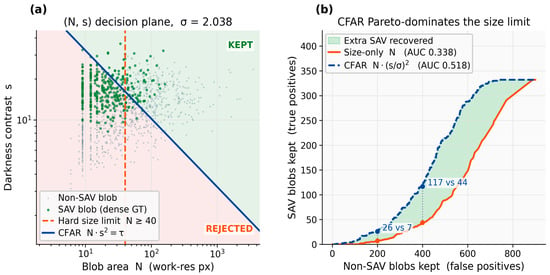
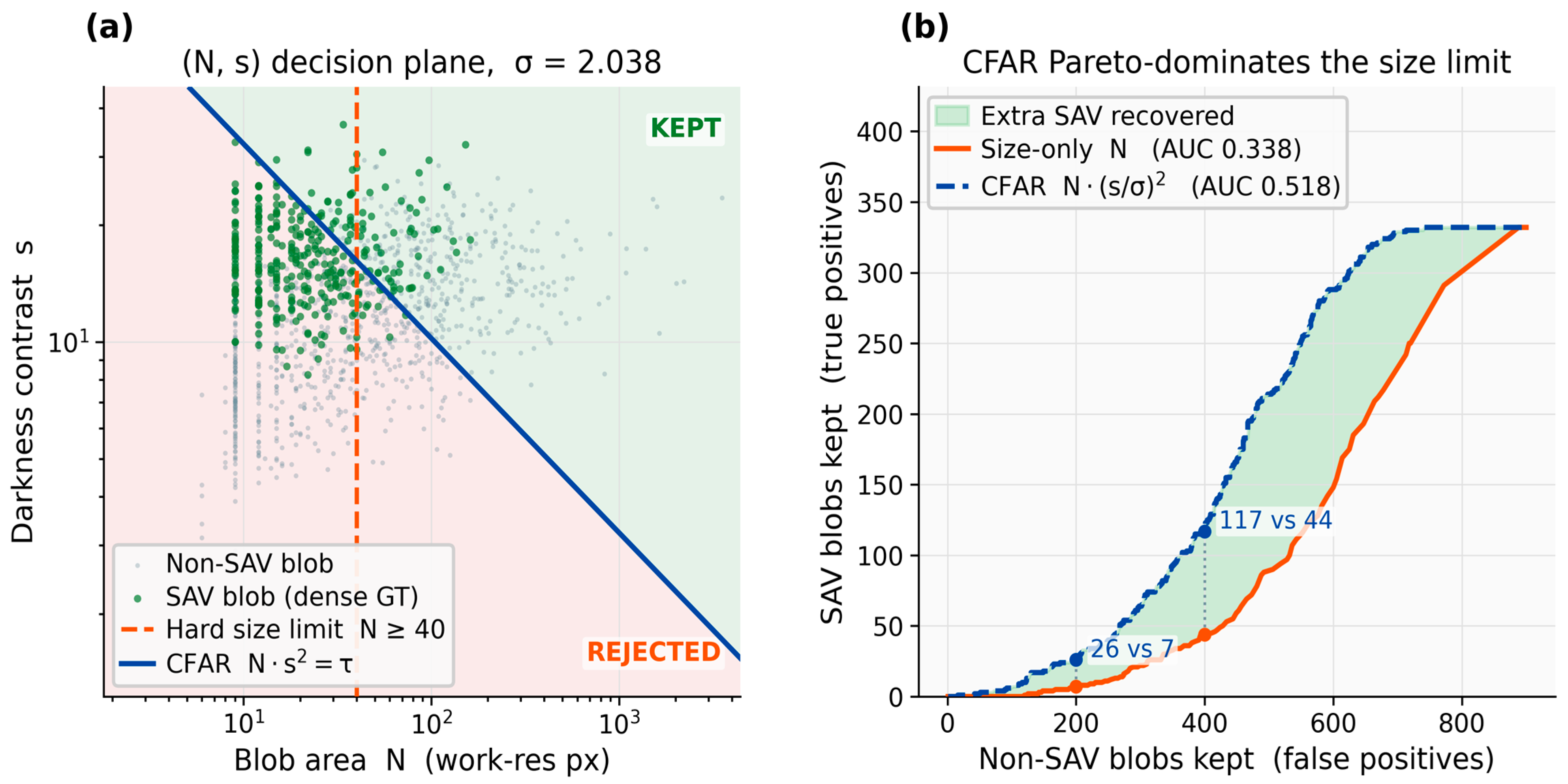
In the plane (Figure 5), real SAV patches occupy a region extending towards small at high . The hard threshold, a vertical line at , removes this small-but-dark population, whereas the CFAR hyperbola retains it while still rejecting small, faint clutter. At matched false-positive budgets, the CFAR statistic keeps substantially more SAV blobs than size alone: for example, at 200 retained non-SAV blobs it keeps 26 versus 7 SAV blobs, and at 400 it keeps 117 versus 44. Ranking quality, measured as the area under the SAV-kept versus non-SAV-kept curve, improves from 0.338 (size-only) to 0.518 (CFAR). The scene clutter used here (2.04) is estimated without labels. These keep-curve comparisons are computed on the dense reference scene; confirming the same Pareto relation across additional densely annotated scenes is left for future work.
Figure 5.
Detectability envelope in the (N, s) plane. (a) The fixed size limit (vertical line) vs. the CFAR boundary, with SAV and clutter blobs and the keep/reject regions shaded. Small but dark SAV, the green blobs lying left of the vertical limit but above the hyperbola, is cut by the fixed limit and kept by the criterion. (b) SAV-kept vs. non-SAV-kept curve, on which CFAR Pareto dominates the fixed size limit.
3.6. The CFAR Operating Point
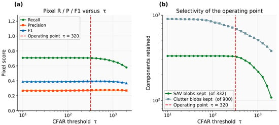
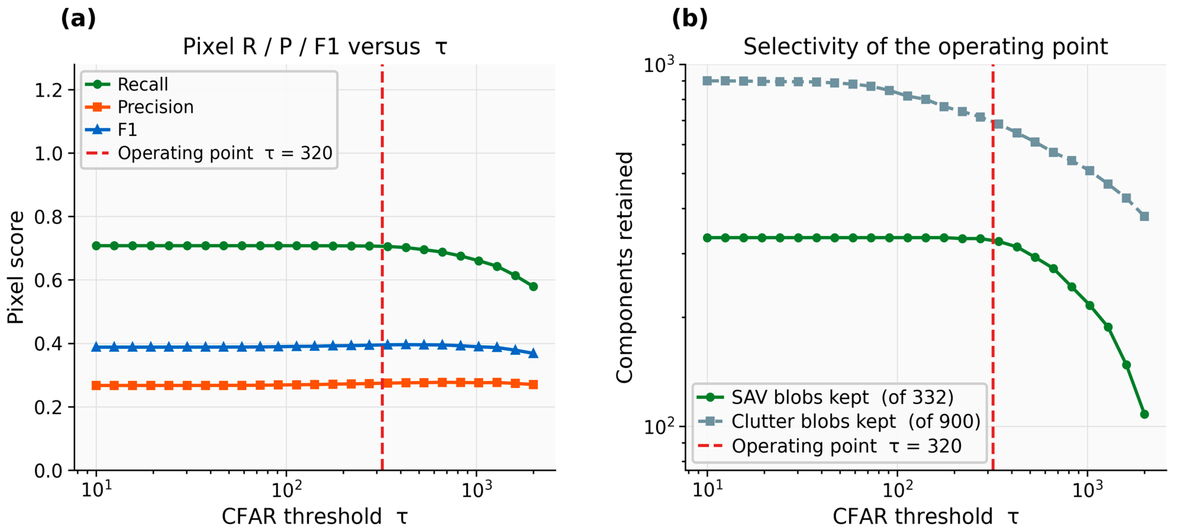
Sweeping (Figure 6) traces a smooth recall–precision trade-off. On the dense reference scene, not one of the 9829 pixels inside the annotated open-water rectangles is flagged at any τ in this range, so the commission rate inside the declared negatives is exactly zero rather than merely small (0 of 9829; 95% upper bound 0.03%), and trades recall against precision on ambiguous detections without saturating the declared negatives. This quantity is measured inside the annotated open-water rectangles and the selected negative classes only. This makes a single, interpretable operating point that can be bound to an external covariate such as measured transparency or the diffuse attenuation coefficient, rather than retuned by hand for each scene.
Figure 6.
CFAR operating point. (a) Recall, precision and F1 as the threshold τ is swept. (b) Selectivity of the operating point: SAV vs. clutter components retained vs. τ, with the false-positive rate inside the annotated open-water rectangles at zero throughout (0 of 9829 pixels at every τ in this range; 95% upper bound 0.03%).
3.7. Deployment Robustness
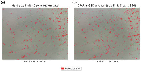
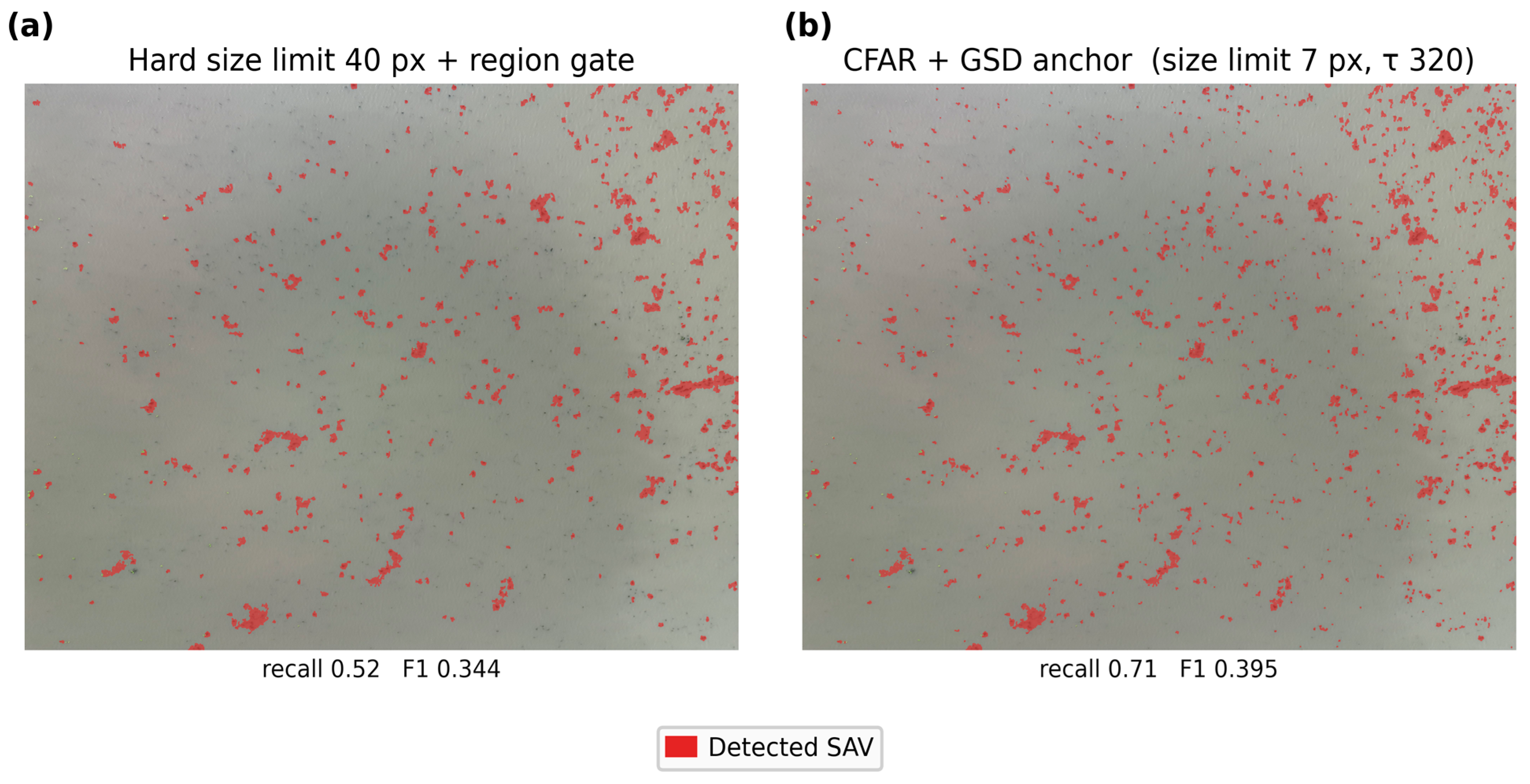
We ran the detector on three deployment images acquired outside the morning window used for calibration, each using its own EXIF metadata to set the physical threshold. Whole-frame predicted coverage stays low on the difficult scenes (green water 4.3%, midday glint 0.44%), in contrast to the 24–25% saturation of a non-adaptive global detector. Because a low coverage value alone cannot distinguish a correct low value from a wrong one, we validated these scenes directly. Six hundred stratified random points (70 in the mapped-SAV class, 60 in a 1 m buffer around it and 70 in the remaining water for each image) were photointerpreted blind and independently twice, and every disagreement plus a 10% audit of the agreements was adjudicated by the authors; agreement between the two independent interpretations was 0.913 (Cohen’s κ = 0.758, and 0.972 on the binary SAV versus not-SAV axis). Estimated with the stratified estimators of Olofsson et al. [43], the mapped SAV class is dominated by commission (Table 4). On the green-water scene the user’s accuracy is 0.129 (95% CI 0.069–0.227) and the estimated true SAV cover is 1.65% (bootstrap 95% CI 0.62–2.93%) against 5.01% mapped, indicating a roughly threefold overestimate of area, with a producer’s accuracy of 0.389. On the same-condition and glint scenes, no sampled point in the mapped class was interpreted as SAV (user’s accuracy of 0.000; 95% upper bound of 0.052). Overall accuracy is high on all three scenes (0.862–0.983) only because SAV is rare and is therefore not an informative metric here. Two mechanisms account for the commission. First, detections concentrate against the boundary of the analysis mask: on the same-condition scene 68% of detected pixels lie within 2 m of an excluded region against 32% of the water area, because bright non-vegetated land such as roads and riprap is not removed by the greenness-and-texture land gate and inflates the local open-water baseline near shorelines. Excluding a 3–4 m boundary band removes 72–100% of the predicted area on those two scenes while changing dense-scene recall by less than 0.001 (0.706 to 0.705) and leaving the open-water scene unchanged, so a larger shoreline exclusion than the 14 px used here is advisable. Second, on the open-water scene, which has no such boundary, commission persists and is not removed by the operating point: raising τ sixteenfold lifts the user’s accuracy only from 0.129 to 0.286 while dense-scene recall falls from 0.706 to 0.434. Sun glint produces specular spikes that are bright rather than dark and yield small, low-contrast candidates, which the statistic does not retain. Predicted coverage was accordingly low in the glint scene tested, but the mapped class there consisted mainly of dark wave troughs and floating-mat edges rather than SAV, and we did not test glint robustness across solar and viewing geometries. For comparison, Figure 7 shows the same whole-frame contrast on the dense reference scene, where exhaustive ground truth is available and both configurations can be scored directly against it.
Table 4.
Deployment-scene point validation. Two hundred stratified random points per scene, 600 in total, were allocated as 70 to the mapped-SAV class, 60 to a 1 m buffer around it and 70 to the remaining water, drawn within the analysis mask and photointerpreted blind and independently twice; every disagreement and a 10% audit of the agreements was adjudicated by the authors. Coverage is given on both denominators because Section 3.7 quotes the whole-frame value while the estimators operate within the analysis mask. Estimates follow the stratified estimators of Olofsson et al. [43]; intervals are bootstrap (10,000 resamples, seed fixed) except where every sampled point was negative, in which case the bootstrap is degenerate and a rule-of-three upper bound is given instead. Producer’s accuracy is undefined where no sampled point was interpreted as SAV. Overall accuracy is 0.862, 0.946 and 0.983 respectively, but it is high only because SAV is rare and is therefore not an informative metric here. On the same-condition scene an estimated 15.6% (10.8–21.2%) of the analysis mask is dry land that the greenness-and-texture land gate fails to exclude, which contributes to its mapped coverage.
Figure 7.
Whole-frame detection on the dense reference scene. (a) Fixed 40 px lower limit on pixel number with the region gate (recall 0.52). (b) GSD-anchored CFAR-inspired detector (recall 0.71). Neither configuration produces false positives inside the annotated open-water rectangles. This figure characterises the reference scene; the deployment scenes are quantified in Table 4.
4. Discussion
4.1. Principal Findings
Three findings follow from the experiments. First, the discriminative axis for SAV in RGB is local-relative darkness rather than greenness; the excess-green (ExG) index performs at chance (AUC 0.438). Second, most SAV is small and falls below the conventional fixed lower limit on pixel number, so a scale-aware minimum unit recovers it: at 4 cm GSD, a fixed 40 px threshold implies a 0.43 m2 minimum patch, below which 73–98% of labelled patches fall across the four densely annotated scenes, and setting the minimum unit correctly raises recall from 0.52 to 0.71 on the full-frame scene, while a size-binned decomposition shows the recovered patches are dark enough and resolved enough to be detected. Third, the lost recall is recoverable without new labels, because a CFAR criterion with scene-estimated clutter and a GSD anchor restores it with no false positives inside the annotated open-water rectangles and outperforms the standard baselines (cross-scene AUC 0.969). We interpret these findings below by relating them to prior RGB and multispectral work, to radiative-transfer theory, and to the limitations of the approach.
4.2. Relation to Prior Work
Our results occupy a specific position relative to three established lines of work, and the comparison clarifies what is gained and what is conceded.
Satellite multispectral and hyperspectral methods map SAV cover synoptically but are bounded by pixel size and water transparency. With Sentinel-2 in low-transparency water, detection is restricted to roughly 1.5–2.0 m depth and cover is retrieved at R2 0.56–0.66 [8], whereas at 3 m PlanetScope resolution low abundances cannot be detected at all [20]. Our 4 cm RGB recovers patches down to about 0.04–0.09 m2, well below these satellite mapping units, so it captures the small, fragmented SAV that coarse pixels miss. The trade-off is explicit: those satellite studies retrieve percent cover, whereas we map presence and extent only.
UAV multispectral methods solve the resolution problem but retain the requirement for red-edge or NIR bands. Object-based workflows classify submerged vegetation at 71–84% accuracy using a near-infrared band [21] and at 77% using a six-band sensor [22]. Hybrid UAV-plus-satellite schemes that report cover and biomass still derive the operational map from a multispectral water index, using the UAV only to generate training samples [27,44]. We obtain comparable or higher cross-scene separability (AUC 0.969) from consumer RGB alone, without calibrated multispectral hardware, again conceding the cover and biomass products that those methods target [15,45,46].
RGB studies addressing submerged targets directly have so far been confined to favourable conditions. Filamentous algae and rooted macrophytes have been classified at 82–92% accuracy, but only in clear, non-turbid rivers with Secchi depth above 2 m [34,35]. RGB-only seasonal monitoring of submerged seagrass was found insufficient to discriminate habitat change, and lowering the flight altitude from 115 to 30 m did not help [36]. Two recent UAV studies frame the comparison further. A feature-pyramid network applied to UAV orthophotos of subtidal and intertidal seagrass in Tokyo Bay reaches 0.957 overall accuracy and 0.918 F1, but it is a supervised deep model trained on exhaustively delineated seasonal ground truth, which is precisely the annotation cost our survey operators ruled out, and it is applied to a tidal flat rather than a turbid inland lake [47]. An amphibious UAV combining aerial and underwater imaging with YOLOv8 reaches mean average precisions of 0.76–0.80, but it does so by submerging the sensor and removing the water column from the optical path, so it answers a different question from ours, which is what can be recovered through the water column from an ordinary consumer RGB camera at altitude [48]. Against both, ours is a label-free detector rather than a trained one, together with the scale-axis analysis that neither study addresses. Our contribution is to extend RGB detection of submerged vegetation into turbid and variable water by keying on local-relative darkness rather than absolute colour, and to address the altitude dependence Prystay et al. [36] encountered by anchoring the scale threshold to GSD rather than changing flight height. The greenness result sharpens the boundary: vegetation indices remain valid for floating and emergent material [30,31], whereas our below-chance ExG AUC localises their failure specifically to submerged targets.
4.3. The Identifiability Map
These findings cohere into an identifiability map with three axes. On the darkness axis, the faintest SAV produces a darkening below the noise floor and is unrecoverable. On the shadow axis, dark SAV and dark shadow are confounded where contrast alone must decide. On the scale axis, small but genuine patches are removed by the size proxy. The decomposition in Section 3.3 separates these cases empirically: the patches missed by the size threshold are not on the darkness axis, because they exceed the candidate threshold, nor lost to resolution, because they survive at working resolution; they are lost to scale alone. The darkness and scale axes are thus separated empirically, whereas the shadow axis is argued from the radiative-transfer model rather than separately quantified here. The central implication is that the scale axis differs in kind from the other two. The darkness and shadow limits are physical lower bounds that require additional spectral information (red-edge, NIR, or shortwave-infrared) to break [8,14,18,49]. The scale limit is an operating-point choice that RGB can correct on its own through anchoring and CFAR. Framing the size threshold as the actionable axis of an identifiability boundary, rather than as a cleanup parameter, is to our knowledge new in SAV remote sensing.
4.4. Radiative-Transfer Interpretation
This map follows directly from how light interacts with submerged vegetation. As the water column deepens or the vegetated fraction within a pixel falls, attenuation drives the bottom signal toward the open-water background, so both the darkening and the residual colour of an SAV pixel weaken together. The full set of observable cues therefore contracts toward the noise floor along a single direction. This contraction is the optical form of the faint-SAV limit, and shadow, which darkens a pixel with almost no change in colour, drives it toward the same point. The darkness and shadow axes are thus physically joined, and neither can be separated from clutter by contrast alone, the same attenuation physics that underpins bio-optical SAV retrievals [15,16] and depth-invariant indices [17]. The scale axis is different in kind: detectability that fails for a single faint pixel can be regained by integrating enough adjacent pixels, which is the role of the CFAR area criterion (Equation (1)), so a patch too faint to cross the per-pixel threshold can still be recovered once its area and contrast are combined. This explains why the scale axis is recoverable whereas the darkness and shadow axes are not.
4.5. Scope and Practical Implications
Within the detectable envelope, RGB supports mapping of SAV presence and, within a stated spatial tolerance, spatial extent. Mapped extent is systematically larger than the annotated extent: on the full-frame reference scene, predicted patch area regresses on annotated patch area with an ordinary-least-squares slope of 1.66 (95% CI 1.28–2.06; robust Theil–Sen 1.33, 1.09–1.57) and an intercept of +0.26 m2 (0.19–0.34), and the predicted total area is 2.9 times the annotated total. Extent should therefore be read as an upper bound unless the boundary halo is corrected, and 42% of annotated polygons are not recovered as discrete objects. It does not support retrieval of cover fraction: cover is confounded with depth and sub-pixel mixing along the same contraction direction, so RGB darkness alone is not expected to recover it, and a formal cover retrieval is beyond the present scope. It also does not resolve the faintest or shadow-occluded SAV. These boundaries imply a clear division of labour. Consumer RGB drones are suited to rapid, low-cost, repeated mapping of where SAV is and how far it extends, including the small, fragmented stands that satellites miss, in clear to moderately turbid water. Multispectral and bio-optical methods remain necessary where cover, biomass, or the deepest and faintest stands are required [15,27,29,38,46,50]. Two design choices make the RGB detector portable. The GSD anchor removes the dependence of a fixed pixel threshold on altitude and camera, so the same physical minimum mapping unit transfers between surveys. The CFAR threshold is retained as a single exposed operating point. We deliberately do not estimate fully automatically from scene clutter, because doing so would require separating SAV specks from clutter specks, precisely the identifiability wall itself, since where SAV is pervasive there is no clutter-only sample. Instead we recommend binding to a measured covariate such as Secchi transparency or the diffuse attenuation coefficient [16,51], consistent with the broader difficulty of transferring fixed thresholds across water conditions reported for multispectral SAV mapping [8,20]. In the single glint scene tested, predicted coverage remained low, but the point validation shows that what was mapped there was mostly dark wave troughs and floating-mat edges rather than SAV, so the detector does not replace dedicated glint-removal preprocessing [52,53,54].
4.6. Limitations
First, the reference standard is expert photointerpretation of 4 cm imagery rather than a synchronous in situ survey. This is a deliberate and, for the present question, sufficient choice rather than a shortfall. Image-based reference is standard practice in optical aquatic remote sensing, where accuracy is routinely assessed against photointerpreted or higher-resolution imagery because co-located field transects cannot be acquired synoptically over large or repeatedly surveyed extents, the same constraint under which satellite SAV products are validated [38]. At 4 cm GSD the drone imagery is itself far finer than the quadrat or point sampling used in most field campaigns, so it serves as a high-resolution reference for the binary detection question rather than as a proxy awaiting ground confirmation. Because every detector is scored against the same annotation, the relative comparison that underlies all of our conclusions is independent of any residual absolute error in the reference. The remaining ambiguity is one of identity, not of detection: at this resolution a dark patch cannot be assigned to species and could in rare cases include floating debris or bottom features, so applications requiring species-level products would add targeted ground checks. Second, the dense scale-axis evidence rests on four exhaustively annotated scenes, all representing the sparse-speck growth form at a single aquaculture site; the coherent-bed regime is represented only by the separate lake masks. Densely annotated scenes spanning more water bodies and growth forms would further test the generality of the size effect, although the patch-size statistic (Table 3) is already consistent across the four scenes. Third, precision is bounded by annotation granularity (0.27 at zero tolerance, rising to 0.57–0.68 within 2–3 px), reflecting dilation halos and residual under-labelling, so the true precision is an interval rather than a point. Fourth, the criterion is applied here as a matched-filter heuristic, and is set empirically rather than calibrated to a nominal false-alarm rate from an explicit clutter model; such a calibration is a natural extension. Fifth, and most consequentially, the point validation of the deployment scenes (Section 3.7) shows that a commission rate which is acceptable where SAV is abundant becomes dominant where SAV is sparse: the detector’s false-alarm area is a few percent of the water surface in every scene examined, which is tolerable against the 1.9% annotated cover of the dense reference scene but is most of what is mapped once true cover approaches zero. Prevalence is therefore a fourth axis of the identifiability map alongside darkness, shadow and scale, and it is not controlled by any parameter the method exposes. Deployment to a water body of unknown SAV cover should be preceded by an independent estimate of prevalence, and predicted coverage alone should not be used as a monitoring indicator. Sixth, although the cross-scene evaluation already spans twelve dates and a range of water levels and clarity within the study region, all imagery comes from a single camera, a single region, and a single flight altitude (~111 m). The GSD anchor’s central claim, that one physical MMU rescales correctly across altitude and camera, is therefore established analytically (Equation (2)) but not yet validated empirically; a multi-altitude, multi-camera acquisition is the single most important next test, alongside cross-region and cross-growth-form transfer [26,55].
5. Conclusions
Consumer RGB drones can map SAV presence and extent within an identifiability envelope set by water-column attenuation, sub-pixel cover, spatial scale and SAV prevalence, provided the discriminative axis is correctly taken to be local-relative darkness rather than greenness. We showed that most SAV is small and is discarded by a conventional fixed lower limit on pixel number, and that a physically anchored, scale-aware minimum mapping unit recovers it and, by construction, rescales with altitude. We corrected it with two label-free mechanisms: a GSD-anchored physical minimum mapping unit, and a CFAR-inspired scale criterion with scene-estimated clutter and a single operating point. The resulting detector outperforms standard greenness, global-darkness, and fixed-MMU baselines while suppressing off-condition flooding, and it requires no re-annotation at deployment. The darkness and shadow limits of RGB remain physical and call for red-edge or NIR information. The scale limit, we have shown, is the axis that RGB can itself repair. Three limitations bound these conclusions. The reference standard is expert photointerpretation of 4 cm imagery rather than a synchronous in situ survey, so what is mapped is image-interpreted SAV-like dark patches rather than field-confirmed SAV. All imagery comes from one lake system, one camera and one nominal flight altitude, so the cross-altitude and cross-camera transfer of the GSD anchor is established analytically but not demonstrated. And the point validation of the deployment scenes shows that a commission rate which is acceptable where SAV is abundant becomes dominant where SAV is sparse, so prevalence bounds operational use as firmly as darkness, shadow and scale do. Future work follows from each of these. Synchronous in situ transects would convert the reference standard from image-interpreted to field-confirmed. A multi-altitude, multi-camera and cross-water-body acquisition would test the GSD anchor empirically rather than analytically. Binding the operating point τ to measured transparency or to the diffuse attenuation coefficient would replace the one remaining hand-set parameter. And an independent estimate of SAV prevalence should precede deployment to any water body of unknown cover, since predicted coverage alone cannot distinguish a correct low value from a wrong one.
Supplementary Materials
The following supporting information can be downloaded at https://www.mdpi.com/article/10.3390/drones10080586/s1: S1. Implementation materials, comprising the detector and baseline code, the figure and analysis scripts, the frozen parameter settings, the train/validation split list, and the annotation files for the lake set, the four exhaustively annotated scenes and the 58-frame cross-scene set, together with the complete deployment-scene point-validation record behind Table 4.
Author Contributions
Conceptualisation, D.X. and Y.F.; methodology, D.X.; software, X.C.; validation, X.C.; formal analysis, X.C.; investigation, D.X. and X.C.; data curation, X.C.; writing—original draft preparation, D.X. and X.C.; writing—review and editing, D.X. and Y.F.; visualisation, X.C.; supervision, D.X. and Y.F.; funding acquisition, D.X. All authors have read and agreed to the published version of the manuscript.
Funding
This research was supported by a project funded by the Priority Academic Program Development of Jiangsu Higher Education Institutions (PAPD), and Project on Health Assessment and Ecological Quality Grading of Municipal Important Wetlands in Suzhou 2026 (JSZC-320500-SZWK-C2026-0126).
Data Availability Statement
The imagery analysed in this study was acquired by, and remains under the data-sharing terms of, the Wetland Ecosystem Field Station of Taihu Lake, National Forestry and Grassland Administration, from which it is available on request. All implementation materials needed to inspect and re-implement the method are provided as Supplementary Material S1: the detector and baseline implementations together with the scripts that generate every figure; the frozen logistic coefficients and standardisation statistics, the region weights, and every threshold setting (candidate probability, tau, minimum pixel count, default minimum mapping unit); the 12/5 training and validation split list for the 17-image lake set; and the annotation files, comprising the 17 dense binary masks of the lake set and the 64 LabelMe files covering the four exhaustively annotated scenes and the cross-scene box set (all annotated frames are included; annotation_summary.csv marks the two excluded from evaluation). S1 also contains the complete record behind Table 4: the sampling design and random seed, the 600 point coordinates, both independent sets of photointerpretations, the adjudication record and the estimation scripts. Because the imagery is not redistributed, S1 supports inspection and re-implementation of the method, and independent scrutiny of every annotation, split and parameter, rather than push-button re-execution of the reported numbers; readers who obtain the imagery from the field station can reproduce them with the supplied code and split lists.
Acknowledgments
We thank Shuai Xue, Fei Shen, and Ziqiang Wang for field assistance and helpful discussions. During the preparation of this manuscript, the authors used ChatGPT (GPT-5.4; OpenAI, San Francisco, CA, USA) for the purposes of language editing, that is, improving the grammar, spelling, and readability of the text. The authors have reviewed and edited the output and take full responsibility for the content of this publication.
Conflicts of Interest
The authors declare no conflicts of interest.
Abbreviations
The following abbreviations are used in this manuscript:
| AUC | Area under the receiver-operating-characteristic curve |
| CFAR | Constant false-alarm rate |
| ExG | Excess-green index |
| EXIF | Exchangeable image file format |
| F1 | F1 score (harmonic mean of precision and recall) |
| GSD | Ground sampling distance |
| HSV | Hue–saturation–value colour space |
| MMU | Minimum mapping unit |
| NIR | Near-infrared |
| OBIA | Object-based image analysis |
| RGB | Red–green–blue |
| SAV | Submerged aquatic vegetation |
| UAV | Unmanned aerial vehicle (drone) |
References
- Renshaw, A. Distribution and Abundance of Submerged Aquatic Vegetation in the Caloosahatchee River Estuary as a Function of Optical Water Quality and Salinity; Florida Gulf Coast University: Fort Myers, FL, USA, 2025. [Google Scholar]
- Jiang, H.; Lu, A.; Li, J.; Ma, M.; Meng, G.; Chen, Q.; Liu, G.; Yin, X. Effects of Aquatic Plant Coverage on Diversity and Resource Use Efficiency of Phytoplankton in Urban Wetlands: A Case Study in Jinan, China. Biology 2024, 13, 44. [Google Scholar] [CrossRef] [Scilit] [PubMed]
- Yang, R.; Wu, J.; Zhao, J.; Guan, Q.; Fan, X.; Zhao, L. Marked Interannual Variability in the Relative Dominance of Phytoplankton over Submerged Macrophytes Rather than Regime Shifts in a Shallow Eutrophic Lake: Evidence from Long-Term Observations. Ecol. Indic. 2024, 166, 112301. [Google Scholar] [CrossRef] [Scilit]
- Zhu, J.; Gong, Z.; Wang, Y. Rapid Response of Aquatic Ecosystems and Environment in Shallow Macrophytic Lakes to Large-Scale Cofferdam Removal. Ecol. Indic. 2025, 178, 113884. [Google Scholar] [CrossRef] [Scilit]
- He, L.; Shi, N.; Guo, S.; Zhang, M.; Chen, B.; Zhou, X.; Wang, H.; Xie, X.; Wan, W.; Cao, T.; et al. Hydrological Alterations Drive Long-Term Decline and Resilience Loss of Submerged Aquatic Vegetation in a Large Floodplain Lake. Freshw. Biol. 2026, 71, e70167. [Google Scholar] [CrossRef] [Scilit]
- Yang, S.; Wan, R.; Yang, G.; Li, B. A Novel Framework to Assess the Hydrological Connectivity of Lake Wetlands in Plain River Networks with Dense Hydraulic Facilities: Comparing Natural and Disturbed States over a Century. J. Hydrol. 2024, 630, 130787. [Google Scholar] [CrossRef] [Scilit]
- Kroth, F.; Kuhwald, K.; Schneider, T.; Oppelt, N. Habitat Suitability and Species Distribution Modelling in Lake Macrophyte Research: A Systematic Review. Ecol. Indic. 2025, 179, 114141. [Google Scholar] [CrossRef] [Scilit]
- Vahtmae, E.; Toming, K.; Argus, L.; Moller-Raid, T.; Ligi, M.; Kutser, T. On the Possibility to Map Submerged Aquatic Vegetation Cover with Sentinel-2 in Low-Transparency Waters. J. Appl. REMOTE Sens. 2023, 17, 044506. [Google Scholar] [CrossRef] [Scilit]
- Vahtmae, E.; Argus, L.; Toming, K.; Moller-Raid, T.; Kutser, T. Assessing Seasonal and Inter-Annual Changes in the Total Cover of Submerged Aquatic Vegetation Using Sentinel-2 Imagery. Remote Sens. 2024, 16, 1396. [Google Scholar] [CrossRef] [Scilit]
- Tompoulidou, M.; Karadimou, E.; Apostolakis, A.; Tsiaoussi, V. A Geographic Object-Based Image Approach Based on the Sentinel-2 Multispectral Instrument for Lake Aquatic Vegetation Mapping: A Complementary Tool to in Situ Monitoring. Remote Sens. 2024, 16, 916. [Google Scholar] [CrossRef] [Scilit]
- Roca-Mora, M.; Peixoto-Dias, C.E.; Vivanco-Bercovich, M.; Lee, C.B.; Fonseca, A.L.; Caballero, I.; Navarro, G.; Horta, P. Blending PlanetScope and Sentinel-2 Imagery to Assess Subtidal Seagrass Changes in Turbid Waters. Mar. Pollut. Bull. 2026, 225, 119228. [Google Scholar] [CrossRef] [Scilit] [PubMed]
- Wilson, K.L.; Wong, M.C.; Devred, E. Comparing Sentinel-2 and WorldView-3 Imagery for Coastal Bottom Habitat Mapping in Atlantic Canada. Remote Sens. 2022, 14, 1254. [Google Scholar] [CrossRef] [Scilit]
- Fabbretto, A.; Bresciani, M.; Pellegrino, A.; Alikas, K.; Pinardi, M.; Padula, R.; Mangano, S.; Giardino, C. Tracking Water Quality and Macrophyte Changes in Lake Trasimeno (Italy) from Spaceborne Hyperspectral Imagery. Remote Sens. 2024, 16, 1704. [Google Scholar] [CrossRef] [Scilit]
- Timmer, B.; Reshitnyk, L.Y.; Hessing-Lewis, M.; Juanes, F.; Costa, M. Comparing the Use of Red-Edge and near-Infrared Wavelength Ranges for Detecting Submerged Kelp Canopy. Remote Sens. 2022, 14, 2241. [Google Scholar] [CrossRef] [Scilit]
- Liu, Y.; Wu, T.; Wang, S.; Gao, Y.; Xia, K.; Wang, X. A Submerged Aquatic Vegetation Biomass Estimation Framework Grounded in Underwater Light Attenuation. Remote Sens. Environ. 2026, 342, 115463. [Google Scholar] [CrossRef] [Scilit]
- Pawar, S.; Goncalves-Araujo, R.; Timmermann, K. In Search of Light: Estimating Diffuse Attenuation Coefficient of Downwelling Irradiance and Its Variation in Optically Complex Shallow Water Habitats Using Sentinel-2 Imagery. Sci. Total Environ. 2025, 965, 178598. [Google Scholar] [CrossRef] [Scilit] [PubMed]
- Hu, C. A Depth-Invariant Index to Map Floating Algae: A Conceptual Design. Remote Sens. Lett. 2024, 15, 1–9. [Google Scholar] [CrossRef] [Scilit]
- Khanna, S.; Hestir, E.L.; Bellvert, J.; Boyer, J.D.; Shapiro, K.D.; Ustin, S.L. A New Index for Detection of Submerged Aquatic Plants under Variable Quality Water: An Extension of the Soil-Line Concept. Giscience Remote Sens. 2024, 61, 2399386. [Google Scholar] [CrossRef] [Scilit]
- Campillo-Tamarit, N.; Molner, J.V.; Soria, J.M. Remote Sensing Tools for Monitoring Marine Phanerogams: A Review of Sentinel and Landsat Applications. J. Mar. Sci. Eng. 2025, 13, 292. [Google Scholar] [CrossRef] [Scilit]
- Rasse, L.; Godfroy, J.; Nogaro, G.; Cordier, F.; Feldis, D.; Meunier, S.; Puijalon, S.; Piegay, H. Monitoring of Riverine Aquatic Vegetation Using Satellite PlanetScope Imagery: Feasibility, Limitations and Prospects. Ecohydrology 2026, 19, e70178. [Google Scholar] [CrossRef] [Scilit]
- Chabot, D.; Dillon, C.; Shemrock, A.; Weissflog, N.; Sager, E.P.S. An Object-Based Image Analysis Workflow for Monitoring Shallow-Water Aquatic Vegetation in Multispectral Drone Imagery. ISPRS Int. J. Geo-Inf. 2018, 7, 294. [Google Scholar] [CrossRef] [Scilit]
- Brooks, C.; Grimm, A.; Marcarelli, A.M.; Marion, N.P.; Shuchman, R.; Sayers, M. Classification of Eurasian Watermilfoil (Myriophyllum Spicatum) Using Drone-Enabled Multispectral Imagery Analysis. Remote Sens. 2022, 14, 2336. [Google Scholar] [CrossRef] [Scilit]
- Husson, E.; Ecke, F.; Reese, H. Comparison of Manual Mapping and Automated Object-Based Image Analysis of Non-Submerged Aquatic Vegetation from Very-High-Resolution UAS Images. Remote Sens. 2016, 8, 724. [Google Scholar] [CrossRef] [Scilit]
- Husson, E.; Reese, H.; Ecke, F. Combining Spectral Data and a DSM from UAS-Images for Improved Classification of Non-Submerged Aquatic Vegetation. Remote Sens. 2017, 9, 247. [Google Scholar] [CrossRef] [Scilit]
- Benjamin, A.R.; Abd-Elrahman, A.; Gettys, L.A.; Hochmair, H.H.; Thayer, K. Monitoring the Efficacy of Crested Floatingheart (Nymphoides Cristata) Management with Object-Based Image Analysis of UAS Imagery. Remote Sens. 2021, 13, 830. [Google Scholar] [CrossRef] [Scilit]
- Novkovic, M.; Cvijanovic, D.; Mesaros, M.; Pavic, D.; Dreskovic, N.; Milosevic, D.; Andelkovic, A.; Damnjanovic, B.; Radulovic, S. Towards Uav Assisted Monitoring of Aquatic Vegetation within Large Rivers-the Middle Danube (Serbia). Carpathian J. Earth Environ. Sci. 2023, 18, 307–322. [Google Scholar] [CrossRef] [Scilit]
- Lu, L.; Luo, J.; Xin, Y.; Xu, Y.; Sun, Z.; Duan, H.; Xiao, Q.; Qiu, Y.; Huang, L.; Zhao, J. A Novel Strategy for Estimating Biomass of Submerged Aquatic Vegetation in Lake Integrating UAV and Sentinel Data. Sci. Total Environ. 2024, 912, 169404. [Google Scholar] [CrossRef] [Scilit] [PubMed]
- Paetzig, M.; Geiger, F.; Rasche, D.; Rauneker, P.; Eltner, A. Allometric Relationships for Selected Macrophytes of Kettle Holes in Northeast Germany as a Basis for Efficient Biomass Estimation Using Unmanned Aerial Systems (UAS). Aquat. Bot. 2020, 162, 103202. [Google Scholar] [CrossRef] [Scilit]
- Fan, Y.; Yang, Z.; Huai, W.; Dai, H.; Zhai, Y. Dynamic Distribution Monitoring and Biomass Estimation of Aquatic Vegetation in Jupia Hydropower Station, Brazil. J. Hydrol.-Reg. Stud. 2024, 51, 101606. [Google Scholar] [CrossRef] [Scilit]
- Kim, K.; Kim, B.-J.; Kim, E.; Ryu, J.-H. Classification of Green Tide at Coastal Area Using Lightweight UAV and Only RGB Images. J. Coast. Res. 2020, 102, 224–231. [Google Scholar] [CrossRef] [Scilit]
- Li, J.; Xing, Q.; Tian, L.; Hou, Y.; Zheng, X.; Arif, M.; Li, L.; Jiang, S.; Cai, J.; Chen, J.; et al. An Improved UAV RGB Image Processing Method for Quantitative Remote Sensing of Marine Green Macroalgae. IEEE J. Sel. Top. Appl. Earth Obs. Remote Sens. 2024, 17, 19864–19883. [Google Scholar] [CrossRef] [Scilit]
- Xing, Q.; Liu, H.; Li, J.; Hou, Y.; Meng, M.; Liu, C. A Novel Approach of Monitoring Ulva Pertusa Green Tide on the Basis of UAV and Deep Learning. Water 2023, 15, 3080. [Google Scholar] [CrossRef] [Scilit]
- Panyawai, J.; Stankovic, M.; Infantes, E.; Cossa, D.; Kaewutai, K.; Prathep, A. RGB and Multispectral UAV Mapping of Dugong Foraging Hotspots and Seagrass Beds in Thailand and Mozambique. Aquat. Mamm. 2025, 51, 464–481. [Google Scholar] [CrossRef] [Scilit]
- Flynn, K.; Chapra, S. Remote Sensing of Submerged Aquatic Vegetation in a Shallow Non-Turbid River Using an Unmanned Aerial Vehicle. Remote Sens. 2014, 6, 12815–12836. [Google Scholar] [CrossRef] [Scilit]
- Kislik, C.; Genzoli, L.; Lyons, A.; Kelly, M. Application of UAV Imagery to Detect and Quantify Submerged Filamentous Algae and Rooted Macrophytes in a Non-Wadeable River. Remote Sens. 2020, 12, 3332. [Google Scholar] [CrossRef] [Scilit]
- Prystay, T.S.; Adams, G.; Favaro, B.; Gregory, R.S.; Bris, A.L. The Reproducibility of Remotely Piloted Aircraft Systems to Monitor Seasonal Variation in Submerged Seagrass and Estuarine Habitats. Facets 2023, 8, 1–22. [Google Scholar] [CrossRef] [Scilit]
- Saura, S. Effects of Minimum Mapping Unit on Land Cover Data Spatial Configuration and Composition. Int. J. Remote Sens. 2002, 23, 4853–4880. [Google Scholar] [CrossRef] [Scilit]
- Hill, V.J.; Zimmerman, R.C.; Byron, D.A.; Heck, K.L. Mapping Seagrass Distribution and Abundance: Comparing Areal Cover and Biomass Estimates between Space-Based and Airborne Imagery. Remote Sens. 2024, 16, 4351. [Google Scholar] [CrossRef] [Scilit]
- Maes, W.H. Practical Guidelines for Performing UAV Mapping Flights with Snapshot Sensors. Remote Sens. 2025, 17, 606. [Google Scholar] [CrossRef] [Scilit]
- Tiskus, E.; Bucas, M.; Gintauskas, J.; Katarzyte, M.; Vaiciute, D. U-Net Performance for Beach Wrack Segmentation: Effects of UAV Camera Bands, Height Measurements, and Spectral Indices. Drones 2023, 7, 670. [Google Scholar] [CrossRef] [Scilit]
- Bertin, E.; Arnouts, S. SExtractor: Software for Source Extraction. Astron. Astrophys. Suppl. Ser. 1996, 117, 393–404. [Google Scholar] [CrossRef] [Scilit]
- Rohling, H. Radar CFAR Thresholding in Clutter and Multiple Target Situations. IEEE Trans. Aerosp. Electron. Syst. 1983, AES-19, 608–621. [Google Scholar] [CrossRef] [Scilit]
- Olofsson, P.; Foody, G.M.; Herold, M.; Stehman, S.V.; Woodcock, C.E.; Wulder, M.A. Good Practices for Estimating Area and Assessing Accuracy of Land Change. Remote Sens. Environ. 2014, 148, 42–57. [Google Scholar] [CrossRef] [Scilit]
- Chen, J.; Yu, Q.; Zhao, F.; Zhang, H.; Liang, T.; Li, H.; Yu, Z.; Zhang, H.; Liu, R.; Xu, A.; et al. Mapping the Fraction of Vegetation Coverage of Potamogeton crispus L. in a Shallow Lake of Northern China Based on UAV and Satellite Data. Remote Sens. 2024, 16, 2917. [Google Scholar] [CrossRef] [Scilit]
- Liu, B.; Sevick, T.; Jung, H.; Kiskaddon, E.; Carruthers, T. Quantifying the Potential Contribution of Submerged Aquatic Vegetation to Coastal Carbon Capture in a Delta System from Field and Landsat 8/9-Operational Land Imager (OLI) Data with Deep Convolutional Neural Network. Remote Sens. 2023, 15, 3765. [Google Scholar] [CrossRef] [Scilit]
- Simpson, J.; Bruce, E.; Davies, K.P.; Barber, P. A Blueprint for the Estimation of Seagrass Carbon Stock Using Remote Sensing-Enabled Proxies. Remote Sens. 2022, 14, 3572. [Google Scholar] [CrossRef] [Scilit]
- Chen, J.; Sasaki, J. Mapping of Subtidal and Intertidal Seagrass Meadows via Application of the Feature Pyramid Network to Unmanned Aerial Vehicle Orthophotos. Remote Sens. 2021, 13, 4880. [Google Scholar] [CrossRef] [Scilit]
- Zhao, F.; Wang, J.; Chen, Y.; Shao, X.; Liu, Y.; Chen, Y.; Xue, F.; Sasaki, J.; Mizuno, K. Cost-Effective Ecological Monitoring in Shallow Waters Using Amphibious Unmanned Aerial Vehicles (AUAV) and Deep Learning-Based Computer Vision. Mar. Environ. Res. 2026, 216, 107911. [Google Scholar] [CrossRef] [Scilit] [PubMed]
- Wang, H.; Li, Y.; Zeng, S.; Cai, X.; Bi, S.; Liu, H.; Mu, M.; Dong, X.; Li, J.; Xu, J.; et al. Recognition of Aquatic Vegetation Above Water Using Shortwave Infrared Baseline and Phenological Features. Ecol. Indic. 2022, 136, 108607. [Google Scholar] [CrossRef] [Scilit]
- Lebrasse, M.C.; Schaeffer, B.A.; Coffer, M.M.; Whitman, P.J.; Zimmerman, R.C.; Hill, V.J.; Islam, K.A.; Li, J.; Osburn, C.L. Temporal Stability of Seagrass Extent, Leaf Area, and Carbon Storage in St. Joseph Bay, Florida: A Semi-Automated Remote Sensing Analysis. Estuaries Coasts 2022, 45, 2082–2101. [Google Scholar] [CrossRef] [Scilit] [PubMed]
- Ellis, E.A.; Allen, G.H.; Riggs, R.M.; Gao, H.; Li, Y.; Carey, C.C. Bridging the Divide between Inland Water Quantity and Quality with Satellite Remote Sensing: An Interdisciplinary Review. Wiley Interdiscip. Rev. Water 2024, 11, e1725. [Google Scholar] [CrossRef] [Scilit]
- Qin, J.; Li, M.; Zhao, J.; Zhong, J.; Zhang, H. Revolutionize the Oceanic Drone RGB Imagery with Pioneering Sun Glint Detection and Removal Techniques. In Proceedings of the 2024 IEEE/CVF Winter Conference on Applications of Computer Vision (WACV), Waikoloa, HI, USA, 3–8 January 2024; pp. 8311–8320. [Google Scholar]
- Gray, P.C.; Windle, A.E.; Dale, J.; Savelyev, I.B.; Johnson, Z.I.; Silsbe, G.M.; Larsen, G.D.; Johnston, D.W. Robust Ocean Color from Drones: Viewing Geometry, Sky Reflection Removal, Uncertainty Analysis, and a Survey of the Gulf Stream Front. Limnol. Oceanogr.-Methods 2022, 20, 656–673. [Google Scholar] [CrossRef] [Scilit]
- Lee, J.-S.; Kim, S.-Y.; Jo, Y.-H. A Novel Method for Eliminating Glint in Water-Leaving Radiance from UAV Multispectral Imagery. Remote Sens. 2025, 17, 996. [Google Scholar] [CrossRef] [Scilit]
- Cvijanovic, D.; Novkovic, M.; Milosevic, D.; Piperac, M.S.; Galambos, L.; Cerba, D.; Stamenkovic, O.; Damnjanovic, B.; Mesaros, M.; Pavic, D.; et al. Conservation and Ecological Screening of Small Water Bodies in Temperate Riverine Wetlands Using UAV Photogrammetry (Middle Danube). Nat. Conserv.-Bulg. 2025, 58, 61–82. [Google Scholar] [CrossRef] [Scilit]

Disclaimer/Publisher’s Note: The statements, opinions and data contained in all publications are solely those of the individual author(s) and contributor(s) and not of MDPI and/or the editor(s). MDPI and/or the editor(s) disclaim responsibility for any injury to people or property resulting from any ideas, methods, instructions or products referred to in the content. |
© 2026 by the authors. Licensee MDPI, Basel, Switzerland. This article is an open access article distributed under the terms and conditions of the Creative Commons Attribution (CC BY) license.