


Highlights
What are the main findings?
- The complete H-PPO model achieved a 100% task success rate and a mean terrain clearance of 771.92 m.
- H-PPO outperformed A* and RRT* in task reliability, mean terrain clearance, and online computational efficiency.
What are the implications of the main findings?
- Hierarchical planning effectively integrates long-horizon route decisions with fixed-wing flight control under dynamic fire and smoke threats.
- Improved safety and reliability are achieved at the cost of longer routes and mission durations.
Abstract
To address the limitations of static-obstacle-based route planning in forest fire missions, this study develops a three-dimensional route-planning method for fixed-wing unmanned aerial vehicles (UAVs) that accounts for time-varying fire and smoke threats, complex terrain, and flight-dynamics constraints. A cellular automaton models fire spread with wind, slope, fuel, and moisture effects, while a Gaussian plume model estimates smoke concentration. The resulting burning and high-concentration smoke cells are encoded as dynamic three-dimensional threat envelopes and local grid masks. A hierarchical proximal policy optimization (H-PPO) architecture then combines a high-level stateful long short-term memory (LSTM) policy for route-subgoal generation with a pretrained low-level flight controller that produces continuous throttle and control-surface commands in JSBSim. In 100 independent simulation tests, the complete H-PPO model achieved a 100% task success rate, a mean terrain clearance of 771.92 m, and an average online decision time of 1.290 ms. Compared with A* and RRT*, H-PPO provided higher task reliability, greater mean terrain clearance, and lower online computational cost. The results show that hierarchical temporal decision making improves safety-prioritized planning in evolving fire and smoke environments, although conservative avoidance increases route length and mission duration. Further real-world and flight-test validation is required.
1. Introduction
Unmanned aerial vehicles (UAVs) are widely used for forest fire monitoring, fire-scene reconnaissance, and emergency response [1]. Unlike routine inspection or transport settings, the flight environment in a forest fire evolves continuously as the fire develops. Flame spread changes no-entry regions, and smoke dispersion expands the area of planning risk [2,3,4]. These changes are jointly affected by wind, terrain, vegetation type, and fuel moisture, so the UAV faces different passable airspace at different times [5,6]. Therefore, route planning for forest fires cannot rely only on static-obstacle assumptions and must account for dynamic flight constraints arising from the combined effects of flames, smoke, and terrain.
In dynamic fire and smoke environments, route safety depends on the relationship among the UAV state, the time of arrival, and threat-field evolution. The same spatial location may pose different risks at different times. A planner must therefore consider both spatial accessibility and time-varying threats. For fixed-wing UAVs, the planned route must also satisfy constraints on speed, altitude, minimum turning radius, climb and descent capability, and executed-trajectory continuity [7,8]. This study therefore formulates route planning in dynamic forest fire environments as a 3D sequential decision problem jointly constrained by fire and smoke threats, complex terrain, and flight dynamics.
Existing UAV route-planning methods generally include graph search, random sampling, artificial potential fields or swarm-intelligence optimization, and deep reinforcement learning [9,10]. A* search algorithm (A*) searches with heuristic costs, whereas rapidly exploring random tree star (RRT*) improves route quality through random sampling and rewiring; both are applicable to path planning [11,12]. In dynamic environments, search-based and sampling-based methods often require periodic replanning as obstacles or risk fields change [9,10]. The performance of artificial-potential-field and swarm-intelligence methods commonly depends on the chosen potential-field or population-update parameters [13,14]. Deep reinforcement learning can learn mappings from continuous observations to control actions and has been used for autonomous UAV navigation and obstacle avoidance in unknown or dynamic environments [15,16,17,18]. For wildfire missions, prior studies investigated dynamic fire-front monitoring, risk-aware routing, reinforcement-learning-based fire-scene surveillance, and fixed-wing fire-front tracking [2,3,4,19,20]. However, the studies reviewed above generally address wildfire monitoring or routing, smoke-risk representation, and fixed-wing trajectory execution as separate problems. Their joint treatment under evolving fire and smoke threats, complex three-dimensional terrain, partial observability, and fixed-wing flight-dynamics constraints remains insufficiently addressed.
For fire-scene modeling, the Rothermel model [5], the Fire Area Simulator (FARSITE) model [21], cellular automata [22,23,24,25,26], and data-driven methods [6,27,28,29] are used to predict fire spread. For smoke dispersion, the Gaussian plume model provides a classical analytical approximation for rapidly estimating concentration distributions from source terms and meteorological conditions [30]. Higher-fidelity Lagrangian or Eulerian frameworks are also used for complex wildfire smoke transport [31,32]. In real wildfire conditions, these estimates are affected by uncertainties in wind fields, fuel properties, fuel moisture, smoke-emission rates, atmospheric stability, and sensing errors, so the resulting threat regions should be treated as time-varying approximations for planning rather than exact forecasts. Although these models describe fire-scene conditions, their outputs are usually represented as 2D state grids, fire-line boundaries, or concentration fields. To support collision checking, safety-margin calculation, and local observation encoding for 3D route planning, the predicted fire-scene outputs must be further organized into an environmental representation suitable for online decision making.
To address these issues, this study develops a 3D route-planning method for fixed-wing UAVs in dynamic forest fire environments. It first constructs a coupled model of fire spread and smoke dispersion to generate time-varying burning-threat regions and high-concentration smoke-threat regions. The fire and smoke states are then organized into 3D dynamic envelopes and local grid masks for threat representation and online planning. On this basis, a hierarchical proximal policy optimization (H-PPO) method incorporating a long short-term memory (LSTM) network is developed. The high-level policy generates relative 3D route subgoals, and a pretrained low-level flight controller tracks the corresponding reference commands, thereby producing routes that satisfy safety and flight-feasibility constraints. In a potential operational implementation, onboard or ground-based observations and meteorological data could be used to update the fire and smoke threat maps, while the generated route subgoals would be executed by the onboard flight-control system. The present study validates this planning-and-control chain only in simulation, and real-flight deployment remains to be evaluated.
This study makes three contributions. First, it establishes a 3D sequential decision-making framework for fixed-wing UAV route planning in dynamic forest fire environments, which incorporates fire and smoke evolution, complex terrain, local observations, and flight-dynamics constraints. Second, it introduces a two-level representation of fire and smoke threats for route planning: 3D dynamic envelopes describe the spatial form of burning and high-concentration smoke threats, whereas local grid masks support online collision checking, safety-margin calculation, and policy observation encoding. Third, it develops a hierarchical PPO planning and control method in which the high-level policy combines local grid observations with LSTM to generate relative 3D route subgoals, while a pretrained low-level flight controller converts the subgoals into continuous throttle and control-surface commands. This design decouples long-horizon route decisions from high-frequency flight control.
The remainder of this paper is organized as follows. Section 2 introduces fire spread, smoke dispersion, and their dynamic threat representations. Section 3 presents the hierarchical PPO planning and control method. Section 4 describes the simulation platform, fire and smoke threat evolution, low-level flight-controller training, high-level route-planning validation, and comparative experiments. Section 5 concludes the paper and discusses limitations and future work.
2. Dynamic Fire and Smoke Threat Modeling and 3D Representation
The fire and smoke environment model provides time-updated burning-threat regions, high-concentration smoke-threat regions, and safety constraints for route planning. It is not treated as an independent fire-forecasting system. Instead, it serves as part of the dynamic fire and smoke environment and generates burning, high-concentration smoke, and terrain threat information that the planner can use. This section first uses a cellular automaton to describe surface-fire spread while incorporating wind, slope, fuel, and fuel-moisture effects. It then couples a smoke-dispersion model to estimate high-concentration smoke-threat regions. Finally, it organizes the discrete fire and smoke states into 3D dynamic envelopes and local grid masks for threat representation, visualization, collision checking, safety-margin calculation, and policy input.
2.1. Basic Cellular Automaton Model
This study uses a two-dimensional surface grid registered to a digital elevation model (DEM) as the cellular space. Each cell represents a geographic surface unit with attributes including elevation, slope, aspect, vegetation type, fuel moisture, and fuel load.
Let the study area be discretized into cells, and let the state of cell at time be defined as
where is the fire state, taking values 0, 1, and 2 to represent unburned, burning, and burned-out states, respectively; is the smoke concentration near the cell center; and is the cumulative burning time of the cell. Smoke-gas temperature is not treated as an independent state variable. Its effect is incorporated into the effective plume source height or model parameters, which avoids retaining a redundant state variable that is not used by subsequent processes.
A Moore neighborhood describes interactions between cells. For an arbitrary target cell , its neighborhood is denoted by , and the set of burning neighbors is
Cell states are updated at every time step . Whether an unburned cell ignites depends on the directional spread rates of burning cells in its neighborhood, whereas a burning cell changes to the burned-out state according to its cumulative burning time.
2.2. Rothermel Fire Spread Rate with Wind and Slope Corrections
At each discrete time step, the cellular automaton determines whether fire can spread from a burning cell to an adjacent unburned cell. The method starts from the no-wind, level-ground base spread rate provided by the Rothermel model [5], then constructs wind and slope correction terms for the cell-to-cell propagation direction to obtain the directional spread rate from source cell to target cell . Wind, slope, and related environmental factors are common determinants in fire-spread modeling [6,22,23,24]. The directional correction functions are constructed with reference to the effects of wind, slope, fuel, and moisture described in the Rothermel formulation and related cellular-automaton fire-spread studies [5,6,22,23,24,25,26,27]. The associated engineering coefficients were adjusted through preliminary simulations to preserve the expected directional effects and numerically stable fire evolution under the adopted discretization.
For a burning cell , the base spread rate under no-wind, level-ground conditions is defined as
where is the reaction intensity, namely the heat released per unit fuel area per unit time; is the propagating-flux ratio; is the dry bulk density of the fuel bed; is the effective heating number; and is the heat required for ignition. These parameters are determined by fuel type, fuel moisture, fuel-bed depth, and fuel surface-area-to-volume ratio and can be obtained from field surveys, remote-sensing retrievals, or geographic information system (GIS) databases.
For source cell and target cell , define the unit propagation-direction vector and the horizontal center-to-center distance as
where and are the horizontal coordinates of the two cell centers. Let be the unit wind-direction vector. The wind correction term is
where is a wind-speed correction coefficient determined by wind speed, fuel type, and fuel packing ratio. This formulation increases the spread rate in the downwind direction, weakens the crosswind effect, and does not provide positive acceleration in the upwind direction.
The slope effect is determined by the elevation difference from the source cell to the target cell. Let
where and are the surface elevations associated with the two cells. The slope correction term is defined as
where is the uphill acceleration coefficient and is the downhill spread-suppression coefficient. This treatment accelerates spread uphill and attenuates spread downhill. To prevent a negative corrected rate, the directional spread rate is finally defined as
where is a numerical lower bound. Before ignition probabilities are calculated, is converted to m/s so that its unit is consistent with the time step .
2.3. State-Transition Probabilities and Model Implementation
The Rothermel model provides a continuous spread rate [5], whereas the cellular automaton updates states at discrete time steps. This study therefore maps the directional spread rate to an ignition probability that increases with the theoretical propagation distance. This idea is consistent with probabilistic cellular fire-spread modeling [23,26,27], while the linear clipping function and the subsequent probability formulation are specific modeling choices adopted here for online simulation. Let the theoretical distance traveled by the fire front along direction during one time step be , and define the linear clipping function as
The single-source ignition probability that burning cell ignites target cell at time is then
where and are vegetation-type and air-humidity correction coefficients for the target cell, respectively. The outer keeps the probability within the interval , preventing invalid probabilities when a correction coefficient exceeds 1.
When a target cell is affected by multiple burning neighbors, this study approximately assumes conditional independence among the ignition events from different neighbors under the given environmental state. The probability that the target cell remains unburned is the product of the probabilities that individual neighbors fail to ignite it. The combined ignition probability is therefore
The state-update rule is
where is a uniform random number and is the complete-burning-time threshold determined by vegetation type and fuel load. The cumulative burning time is updated as follows. When a cell ignites, ; when a cell remains burning, ; and when a cell is unburned or burned out, its cumulative burning time remains unchanged or is no longer updated.
2.4. Smoke Dispersion Model and Coupling
High-concentration smoke-threat regions constitute a dynamic route threat distinct from burning-threat regions and may cover a larger area. To obtain a low-cost concentration approximation that updates synchronously with the cellular-automaton state, this study uses a Gaussian plume model to estimate smoke concentration [30]. Lagrangian or Eulerian dispersion frameworks can also provide higher-fidelity representations of complex wildfire smoke transport [31,32]. The Gaussian approximation is selected here to support online environmental updates during planning. However, the Gaussian plume model assumes simplified and approximately steady meteorological conditions and does not explicitly capture transient turbulence, terrain-induced airflow, spatially varying wind fields, or complex fire–atmosphere interactions. Therefore, the predicted smoke distribution is used as a computationally efficient approximation of high-concentration smoke-threat regions for route planning rather than as an accurate forecast of real wildfire smoke transport.
At each time step, all burning cells are treated as continuous point sources. Let the smoke emission rate of source cell be , the mean wind speed be , and a local coordinate system be defined by the wind direction. In this system, is the downwind distance from the source to the target point and is the crosswind distance. For a downwind target point satisfying , the smoke-concentration contribution from source at location is
where and are the lateral and vertical dispersion coefficients, which are typically determined by downwind distance and atmospheric stability; is the effective source height. The effective source height is approximated as the sum of flame height and thermal-rise height, namely
In the present implementation, all experiments use a fixed distance-dependent parameterization: and are set to and , respectively, where is selected from 100 uniformly spaced downwind-distance values over 1–5000 m. The lookup index is obtained by dividing by the 50 m environmental-grid interval, taking the integer part, and limiting the result to the range 0–99. Accordingly, ranges from 0.1 to 500 m and ranges from 0.05 to 250 m. No separate atmospheric-stability class is switched between scenarios, and the same parameterization is used in all comparative experiments.
The total smoke concentration in any cell is obtained by summing the contributions from all burning cells:
where is the set of burning cells at time . When smoke concentration exceeds the planning safety threshold , the cell is marked as a high-concentration smoke-threat cell:
where is the indicator function. In the implementation, each Gaussian-plume contribution is multiplied by 1 before the contributions from all burning cells are superimposed. Therefore, in the thresholding operation denotes the resulting simulation concentration index rather than a field-calibrated smoke concentration. A cell is classified as a high-concentration smoke-threat cell exactly when . This fixed engineering cutoff converts the continuous simulated plume into a binary threat mask and excludes the low-value tail of the Gaussian plume from the no-fly region. The resulting mask is used consistently for high-level policy observation, collision checking, safety-margin calculation, and trajectory evaluation. The value 50 was not calibrated against field smoke measurements, visibility observations, medical exposure limits, or aviation operating standards and therefore has no direct real-world safety interpretation. Throughout this paper, “high-concentration smoke” refers only to cells exceeding this cutoff in the simulated concentration field. All planning algorithms use the same concentration calculation and threshold.
2.5. 3D Dynamic Representation of Fire and Smoke Threats
The cellular automaton outputs discrete burning states and smoke-concentration grids. To characterize the spatial form of threats in continuous flight space, this study extracts burning cells and high-concentration smoke cells to construct 3D dynamic fire and smoke envelopes. The local grid masks corresponding to the same fire-scene state are retained for online planning. The two representations arise from the same dynamic environmental state but serve different functions. Unless otherwise specified, the area formed by burning cells is termed the burning-threat region, and the area where smoke concentration exceeds the safety threshold is termed the high-concentration smoke-threat region. Together, they are referred to as the fire and smoke-threat regions. The active burning region and cumulative burned region are used only to describe fire-evolution results and correspond to the sets of burning and burned-out cells, respectively.
Let the sets of burning-threat cells and smoke-threat cells be
For each threat cell, construct a ground point and an upper-boundary point. The threat point set is defined as
where denotes threat height. For burning cells, it can be determined by flame height or a vertical safety margin. For smoke cells, it can be determined by the effective plume source height or a specified smoke hazard height. The 3D dynamic fire and smoke envelope is given by the convex hull of the point set:
where denotes the 3D convex-hull operation. The convex hull can be represented by vertices, facets, and their adjacency relations for spatial-form analysis and 3D visualization of the threat region.
However, when a burning-threat region or high-concentration smoke-threat region contains disconnected components, a single convex hull may enclose safe gaps between them. The present implementation does not construct connected-component-wise or other subregional convex hulls. Instead, the 3D convex hull is used only for spatial-form analysis and visualization. Online collision checking and safety-margin calculation operate on the cell-wise burning and high-concentration smoke masks of the environmental grid, while the high-level policy receives UAV-centered local samples of these masks.
The local grid observation used by the high-level policy is defined as
where is the UAV-centered local terrain-elevation map, is the burning-threat cell mask, is the high-concentration smoke-threat cell mask, and is the task-boundary validity mask. Thus, the 3D dynamic fire and smoke envelopes describe threat spatial form, whereas the environmental-grid masks and their UAV-centered local samples support online collision checking, safety-margin calculation, and policy-observation encoding.
Figure 1a,b shows how the same dynamic environmental state is represented by a 3D envelope for spatial-form visualization and by a UAV-centered four-channel grid for policy observation. Figure 1c,d further quantifies the over-enclosure caused by applying one global convex hull to a representative snapshot containing four disconnected threat components. The cell-wise threat footprint is 0.86 km2, whereas the global-hull footprint is 8.02 km2. The global hull therefore falsely encloses 7.15 km2, corresponding to 89.2% of its footprint, including safe space between the disconnected components. The cell-wise masks preserve this space and are used for online planning instead of either the global hull or a set of subregional hulls.
Figure 1.
Complementary representations of a dynamic fire and smoke environment and illustration of global convex-hull over-enclosure. (a) 3D dynamic threat envelope; (b) UAV-centered four-channel local observation grid; (c) horizontal footprint of a single global convex hull for a representative disconnected-threat snapshot; and (d) corresponding cell-wise online threat mask. The dashed rectangle in (a) denotes the local sampling window, blue triangles in (a,b) indicate the UAV position, and yellow stars in (c,d) indicate ignition sources.
3. 3D Route Planning in Dynamic Fire and Smoke Environments Using Hierarchical PPO
3.1. Route-Planning Problem Definition
Given the dynamic fire and smoke environment model in Section 2, fixed-wing UAV route planning is formulated as a sequential decision problem in a dynamic 3D environment. Given a start point, target region, terrain elevation, and time-updated burning and high-concentration smoke threats, the high-level route planner must guide the UAV to the target region within the task time limit while avoiding terrain, burning-threat regions, and high-concentration smoke-threat regions. Because a fixed-wing UAV cannot hover or turn in place like a multirotor UAV, the executed trajectory must also satisfy dynamic constraints on speed, altitude, minimum turning radius, climb and descent capability, and trajectory continuity.
This study does not assume that the planner has access to the complete future fire and smoke threat state. At each high-level decision time, the route planner receives only the current UAV navigation state and a UAV-centered local grid observation. The local grid observation contains terrain elevation, burning-threat cells, high-concentration smoke-threat cells, and task boundaries, which describe environmental constraints within the currently observable range. The high-level planner uses this information to generate a bounded relative 3D route subgoal, and the low-level flight controller tracks the corresponding reference altitude, speed, and heading while the subgoal remains valid.
Let the UAV state be , the control input be , the dynamic environment state be , the target point be , and the task time limit be . The objective is to maximize the probability of reaching the target within finite time while reducing collision risk, route length, task duration, and excessive maneuvers. A feasible executed trajectory must satisfy
where denotes terrain-inaccessible regions, and and denote the burning-threat and high-concentration smoke-threat regions at time , respectively. , , , and denote altitude, speed, roll angle, and climb or descent rate, respectively. The problem has a long horizon, continuous controls, and partial observability. To reduce the difficulty of direct end-to-end control learning, this study uses a hierarchical structure that decouples low-frequency route-subgoal generation from high-frequency flight-dynamics control [33,34].
3.2. Overall Hierarchical Planning and Control Architecture
Fixed-wing UAV route planning in dynamic fire and smoke environments involves long horizons, partial observability, and continuous dynamic constraints. This study therefore uses a hierarchical planning and control architecture that combines high-level route decisions with low-level flight tracking. The architecture comprises a high-level route planner, a route-subgoal-to-command conversion module, a low-level flight controller, a dynamic fire and smoke environment, and the JSBSim six-degree-of-freedom flight-dynamics model. At a low decision frequency, the high-level policy selects the route subgoal for the next phase. At a higher control frequency, the low-level flight controller converts that subgoal into executable reference altitude, speed, and heading commands and outputs continuous throttle, aileron, elevator, and rudder commands. This hierarchy decouples long-horizon route selection from high-frequency flight-dynamics control, allowing the high-level policy to focus on safe route decisions under dynamic fire and smoke threats and complex terrain rather than learning complex control-surface dynamics directly. The interaction among the dynamic environment, the high-level route planner, the low-level flight controller, and the JSBSim flight-dynamics model is illustrated in Figure 2.
Figure 2.
Hierarchical planning and control architecture for fixed-wing UAV route planning in dynamic fire and smoke environments.
For clarity, the module that generates route subgoals is termed the high-level route planner, and its learned mapping is termed the high-level policy. The module that tracks reference commands is termed the low-level flight controller, and its learned mapping is termed the low-level control policy. The flight curve generated by the JSBSim dynamics model is referred to as the executed trajectory.
At the -th high-level decision time , the high-level policy receives the current navigation state, the local grid observation, and the recurrent hidden state from the previous decision time, forming the high-level observation
where is the navigation vector containing UAV position, velocity, and target-relative information, and is the four-channel local grid observation centered on the UAV. As shown in Figure 2, contains terrain elevation, burning-threat, high-concentration smoke-threat, and task-boundary-validity information. The high-level Actor outputs a three-dimensional continuous action conditioned on the LSTM hidden state
After scaling, boundary enforcement, and altitude clipping, the action yields the 3D route subgoal relative to the current UAV position. Thus, the high-level action does not directly correspond to control-surface or throttle commands. Instead, it identifies the local spatial position that the UAV should prioritize during the next planning phase.
Let the set of low-level control steps corresponding to high-level action segment be
where denotes the initial low-level control step of the action segment and denotes its actual duration in low-level control steps. Under normal conditions, equals the preset high-level decision interval. If the UAV reaches the route subgoal early, collides, enters the target region, or reaches the task time limit, the current action segment terminates early. The high-level policy can therefore regenerate the route subgoal according to the actual flight state and environmental changes rather than continuing to execute an invalid subgoal.
Within action segment , the route subgoal remains unchanged, but the low-level reference commands are updated in real time according to the current UAV state. Specifically, let denote the route subgoal, and let denote the current UAV position. The route-subgoal-to-command conversion is defined as
where , , and denote the reference altitude, reference speed, and reference heading, respectively. The reference speed is fixed at . The heading angle is measured clockwise from north; therefore, takes the eastward and northward position differences as its first and second arguments, respectively. When the horizontal distance between the UAV and the route subgoal is negligible, the current heading is retained.
The low-level flight controller then forms the low-level observation from the tracking errors between the reference commands and the current UAV states, together with the attitude, angular rates, and aerodynamic states, and outputs continuous control inputs
where
where , , , and denote the throttle, aileron, elevator, and rudder control inputs, respectively. The tracking errors are calculated from the differences between the reference and current altitude, airspeed, and heading states; the heading error is wrapped to the interval . The JSBSim six-degree-of-freedom flight-dynamics model propagates the UAV state:
JSBSim updates the state using a small physical integration step. The low-level flight controller updates control commands at a fixed control period, whereas the high-level policy generates a new route subgoal after multiple low-level control periods.
As shown in Figure 2, the dynamic fire and smoke environment evolves continuously with simulation time and receives the executed UAV state for collision checking, safety-margin calculation, and task-state updates. During low-level control, the environment module performs collision checking, safety-margin calculation, and task-state updates using the UAV position, terrain elevation, burning-threat regions, and high-concentration smoke-threat regions. At each new high-level decision time, the system reconstructs the local grid observation from the latest fire and smoke threat state. The high-level policy therefore makes decisions from information within the currently observable range and does not assume access to complete future fire and smoke threat evolution.
To ensure that the route subgoals learned by the high-level policy are practically executable, the low-level flight controller is first pretrained on an independent command-tracking task, and its parameters remain fixed during high-level policy training and deployment.
3.3. Low-Level Flight Controller
The low-level flight controller is pretrained with a PPO control policy [35]. Its task is not to avoid fire and smoke threats but to stably track the reference altitude, speed, and heading associated with the high-level route subgoal while outputting continuous throttle and control-surface commands.
The low-level control-policy network contains two Tanh fully connected hidden layers, each with a width of 256. After pretraining, its parameters remain fixed. The same low-level flight controller is reused during execution by H-PPO, A*, and RRT* so that all high-level route-planning algorithms operate under identical dynamic execution conditions.
3.3.1. State Space
The low-level control observation consists of reference-command tracking errors, UAV attitude, angular-motion states, and aerodynamic states:
Table 1 defines the low-level control-state variables and their units. To maintain numerically compact and comparable input magnitudes, the altitude-related variables are expressed in kilometers, while the airspeed error is represented as a dimensionless value scaled by the reference speed of 60 m/s.
Table 1.
State space of the low-level flight controller.
3.3.2. Action Space
The low-level action space contains four normalized continuous control inputs: throttle, aileron, elevator, and rudder.
The throttle input is normalized to [0, 1], whereas the aileron, elevator, and rudder inputs are normalized to [−1, 1].
3.3.3. Reward Function and Independent Pretraining
To provide dense feedback for the continuous tracking task, the low-level flight controller uses the following reward function based on altitude, speed, and heading errors:
The coefficient 20 was selected through preliminary tracking trials to provide sufficiently discriminative feedback as the combined altitude, speed, and heading errors increase. The pretrained low-level controller and its reward settings were subsequently fixed and used consistently for all high-level planning methods.
An episode terminates when flight altitude falls below or the control horizon reaches 500 steps. This reward is used only for independent training of the low-level flight controller; the low-level parameters remain fixed during high-level route-planning training.
3.4. High-Level Route-Planning Model
The high-level policy outputs a relative 3D route subgoal at each discrete decision time. To ensure a fair comparison, H-PPO, A*, and RRT* all receive the same UAV-centered local grid observation and update route subgoals at the same high-level decision period of .
3.4.1. High-Level State Space and Local Grid Observation
The high-level route-planning observation consists of a 10-dimensional navigation vector and a four-channel local grid observation:
where is the normalized 3D UAV position, is the normalized three-axis velocity, is the normalized relative position vector to the final goal, is the normalized 3D distance to the final goal, and is the local grid observation. The local grid has a horizontal resolution of 100 m and covers a UAV-centered area of 4.1 km × 4.1 km. This resolution refers only to horizontal environmental sampling; the proposed H-PPO method does not construct a vertically voxelized occupancy grid, and the UAV altitude is represented as a continuous variable. Its four channels represent normalized terrain elevation, the burning-threat cell mask, the high-concentration smoke-threat cell mask, and the task-boundary validity mask.
The 100 m local observation is reconstructed online from the underlying 50 m terrain, burning-state, and smoke-concentration grids at each high-level decision time. Specifically, the centers of the local cells are placed at 100 m intervals relative to the current UAV position. Each local-cell center is transformed into world coordinates and mapped to the containing 50 m source cell by dividing its horizontal coordinates by 50 m and taking the integer part. The terrain elevation and the corresponding burning and smoke states are then copied from that source cell. Terrain elevation is normalized by the maximum flight altitude of 6000 m, while burning and high-concentration smoke states are encoded as binary masks. Samples outside the 5 km × 5 km task area are marked in the boundary-validity channel. No spatial averaging or interpolation is applied during this coordinate-based resampling. The coarser local resolution was selected to balance the spatial observation range and policy-network input size, and the same mapping procedure is used by H-PPO, A*, and RRT*. The components and dimensions of the high-level route-planning state space are summarized in Table 2.
Table 2.
Components of the high-level route-planning state space.
3.4.2. Feature Fusion and LSTM
The navigation vector is encoded by a 64-dimensional fully connected layer, LayerNorm, and a Tanh function. The local grid observation is encoded as a 512-dimensional feature by a three-layer convolutional network followed by adaptive average pooling. The two features are concatenated and mapped to a 128-dimensional fused feature . To model temporal dependencies across decisions in fire and smoke threat evolution and UAV motion, the fused feature enters an LSTM with a hidden dimension of 128 [36,37]. The hidden state and cell state are propagated throughout an episode and reset only when the episode is initialized or terminated.
The Actor network takes as input and outputs the mean of a three-dimensional Gaussian distribution and a trainable log standard deviation. The Critic network outputs the state value . During training, the initial recurrent state is stored for each continuous high-level decision sequence, temporal order is preserved within each sequence during updates, and truncated backpropagation through time optimizes the recurrent network. Terminal samples do not bootstrap values, which avoids hidden-state leakage across episodes. The detailed Actor–Critic network architecture is summarized in Table 3.
Table 3.
Actor–Critic network architecture of the high-level route-planning model.
3.4.3. Action Space for High-Level Route Subgoals
The high-level Actor outputs a three-dimensional continuous action . After scaling, the action yields the route-subgoal displacement relative to the current position:
The horizontal magnitude of the route-subgoal displacement is limited to 1500 m, and the altitude increment is limited to ±300 m. The altitude coordinate is represented continuously within the range [100, 6000] m and is not divided into fixed vertical layers. The ±300 m value denotes the maximum relative altitude displacement of a route subgoal generated at one high-level decision time, rather than a vertical discretization interval. The route subgoal must remain at least 500 m from the horizontal task boundary. The high-level decision period is 10 s, while the low-level controller and JSBSim update the executed flight state at 0.2 s and 0.01 s intervals, respectively. Therefore, the executed altitude trajectory evolves continuously under the flight-dynamics constraints.
The maximum horizontal route-subgoal displacement of 1500 m and the horizontal boundary margin of 500 m were determined from the local-observation geometry and the aircraft minimum turning radius, whereas the vertical displacement bound of ±300 m was selected according to the aircraft climb/descent capability and terrain-clearance requirements. Specifically, the aircraft-centered 41 × 41 local grid contains 20 cell-center intervals in each horizontal direction. At a resolution of 100 m, the distance from the center to the outermost cell center is 2000 m. Limiting the horizontal route-subgoal displacement to 1500 m therefore leaves a 500 m margin within the represented local region. This margin equals the configured minimum turning radius of the aircraft; consequently, 500 m is also used as the minimum distance between a route subgoal and the horizontal task boundary. At the reference speed of 60 m/s, a displacement of 1500 m corresponds to approximately 25 s of horizontal look-ahead, so the route subgoal provides guidance over multiple high-level decision periods rather than specifying a position that must be reached within one period. The ±300 m vertical displacement bound allows the high-level policy to command terrain-clearance adjustments while preventing excessively large changes in the reference altitude. Given the maximum climb and descent rates of 10 and 8 m/s, respectively, a 300 m altitude change requires at least 30 and 37.5 s, corresponding to approximately three to four high-level decision periods. The 1500 m horizontal displacement limit, ±300 m vertical displacement bound, and 500 m boundary margin are kept fixed across all H-PPO training and evaluation scenarios.
3.4.4. Composite Reward Function for High-Level Route Planning
The high-level route-planning reward comprises task progress, terminal events, safety margin and route-subgoal progress. Let be the 3D distance from the UAV to the final goal and be the reduction in goal distance between adjacent control times. The base reward is defined as
where , , and indicate task success, collision, and timeout, respectively. To prevent the agent from obtaining sustained positive reward by remaining in a safe area, safety shaping uses the difference in the safety potential function between adjacent states. Let , , and denote the clearances from the UAV to fire and smoke threats, terrain, and the task boundary, respectively. Specifically, is calculated as the minimum three-dimensional Euclidean distance between the UAV and the vertically extended volumes of all burning-threat and high-concentration smoke-threat cells in the current local grid. The vertical extent of each threat cell is defined from the local terrain surface to its corresponding threat height. The terrain clearance is calculated as the vertical difference between the UAV altitude and the DEM elevation at the current horizontal position. The boundary clearance is the minimum horizontal distance from the UAV to the four boundaries of the task area. The corresponding reference margins are , , and . Define
The first term rewards improvement in the safety potential function, and the second applies a quadratic penalty when a clearance falls below its reference margin. The route-subgoal progress reward is defined as
The return for a high-level action segment consists of all low-level control-step rewards accrued during the segment
The reward weights were selected through preliminary training trials to establish a safety-prioritized hierarchy among task completion, global progress, safety clearance, and route-subgoal tracking. The terminal rewards of +260 for success and −260 for collision were assigned the largest magnitudes so that successful completion and collision avoidance dominate policy learning. The timeout penalty of −120 distinguishes failure to complete the mission from direct collision. The goal-progress coefficient of 2.0 provides dense guidance toward the final goal, whereas the safety-margin penalty coefficient of 0.01 and route-subgoal progress coefficient of 0.05 provide local shaping without overwhelming the terminal objective and global progress reward. The same weights were used in all corresponding training and evaluation runs and are not claimed to be universally optimal. The contribution of the additional safety-potential and route-subgoal progress terms is evaluated through the ablation study in Section 4.4.
To prevent extreme rewards from destabilizing policy updates, the cumulative reward in an episode is clipped to .
3.5. PPO Algorithm
Both the low-level flight controller and the high-level route planner use proximal policy optimization (PPO) as the primary training framework [35]. Both policies use an Actor–Critic architecture and online data sampled under the current policy, but their decision granularity and training objectives differ. The low-level control policy learns continuous tracking of reference altitude, speed, and heading at the control-step level. The high-level policy learns to generate relative 3D route subgoals from local fire and smoke observations at the action-segment level. Training was conducted in two stages. The low-level controller was first pretrained using five parallel environments for a fixed budget of 5.0 × 10⁶ control steps. Because a low-level episode could terminate before reaching its maximum horizon of 500 control steps, the number of completed low-level episodes was not prescribed in advance. After pretraining, the low-level controller parameters were frozen. Each high-level model was then trained for a fixed budget of 2000 episodes using six parallel environments. Each high-level episode randomly selected one of the three terrain scenarios and terminated when the UAV reached the goal, collided with a threat or the task boundary, or completed 1500 low-level control steps, corresponding to 300 s of simulated flight. Six episode rollouts were normally collected under the current policy before each PPO update, and the route subgoal was updated every 50 low-level control steps, corresponding to 10 s. Neither training stage used an adaptive early-stopping rule. Checkpoints were saved during high-level training, and the checkpoint with the highest composite monitoring score based on return, task success, collision, and goal-distance indicators was retained for subsequent independent evaluation.
PPO limits the magnitude of each update between the old and new policies, thereby suppressing excessive policy drift while retaining the capacity for policy improvement. For any sample , the probability ratio between the new and old policies is defined as
The clipped policy objective is
where is the advantage estimate and is the clipping coefficient. This study uses generalized advantage estimation (GAE) to compute the advantage function [38]:
where is the temporal-difference error.
The value network is typically fitted to the target value function by minimizing the mean squared error:
where is generally computed from the discounted cumulative return.
To encourage exploration, the objective also includes an entropy regularization term:
The policy loss, value-function error, and entropy regularization jointly define the optimization objective:
4. Simulation Experiments and Results Analysis
4.1. Simulation Platform and Experimental Setup
4.1.1. Simulation Environment
To evaluate the proposed hierarchical PPO route-planning method in dynamic fire and smoke environments, this study constructs a simulation platform that includes the dynamic fire and smoke environment model, local grid observations, fixed-wing flight dynamics, and multiple high-level route-planning algorithms. The high-level route-planning policy and conventional planning algorithms are implemented in Python 3.8 and PyTorch 2.4.1, and flight dynamics are computed using the C172x six-degree-of-freedom model in JSBSim [39]. All experiments were conducted on a workstation equipped with an Intel Core i7-14700 CPU and an NVIDIA GeForce RTX 3090 GPU. The online decision times reported in the comparative experiments were measured on this hardware platform.
The task area is 5 km × 5 km, with a terrain-grid resolution of 50 m. The low-level control period is 0.2 s, and the maximum task duration per episode is 300 s. In route-planning experiments, fire and smoke threat states update every 1 s. At each high-level decision time, the system reconstructs the local grid observation from the current UAV position and the latest fire and smoke threat state.
The experiments include valley, ridge, and multi-peak dynamic fire and smoke scenarios. The valley scenario evaluates local route selection in constrained passages. The ridge scenario evaluates detour capability under large-scale elevation changes and directional fire and smoke dispersion. The multi-peak scenario combines complex terrain relief with fragmented threat regions and evaluates overall planning capability in a multi-constraint environment. During training, each episode randomly selects one of the three terrain types and reinitializes the terrain, fire and smoke state, and UAV state. The terrain-resolved evaluation was conducted using 30 independent episodes for each model in each terrain scenario, giving 90 test episodes per model. The same random seeds (42–71) were used across models within each scenario, and the terrain, fire and smoke state, and UAV state were reinitialized for each episode.
4.1.2. Evaluation Metrics
To evaluate the planning algorithms comprehensively, this study reports task success rate, mean terrain clearance, fire and smoke threat-avoidance success rate, average decision time, average task duration, average route length, average executed-trajectory curvature, and maximum roll angle. Task success rate measures the ability to reach the target region safely within the time limit. Mean terrain clearance is the time average of the vertical distance between the UAV and terrain along each executed trajectory. The minimum safety margin is defined as the trajectory minimum of the smaller of the terrain clearance and the fire/smoke-threat clearance. The fire and smoke threat-avoidance success rate is the proportion of flights that do not enter burning-threat or high-concentration smoke-threat regions. Average decision time is the time required for one high-level policy inference or one replanning operation, excluding the offline training cost of reinforcement learning. Average task duration and average route length reflect execution efficiency, whereas average executed-trajectory curvature and maximum roll angle evaluate trajectory smoothness and the executability of the fixed-wing UAV.
When an algorithm fails to complete a task, the reported task duration, route length, executed-trajectory curvature, and maximum roll angle are computed from the actual executed trajectory from the start point to the termination time of that episode. Episodes terminate when the target is reached, a collision occurs, or the task time limit is reached.
For the terrain-resolved ablation-model evaluation, each model was evaluated in 90 episodes, comprising 30 independently seeded episodes in each of the valley, ridge, and multi-peak scenarios. The same terrain and random-seed combinations were used for all four models. Continuous metrics are reported as the mean ± standard deviation for each terrain and over all 90 episodes. For the planning-algorithm comparison, each algorithm was evaluated in 100 independently seeded episodes, with the three scenarios assigned cyclically, and continuous metrics are reported as arithmetic means over the 100 episodes. Because task success and fire and smoke threat avoidance are binary outcomes, their sampling uncertainty was quantified using Wilson 95% confidence intervals. Success differences between successive ablation models were assessed using two-sided exact paired McNemar tests because their episodes were matched by terrain and random seed. Planning-algorithm success proportions were compared using two-sided Fisher’s exact tests. Holm correction was applied separately to the ablation-model and planning-algorithm comparison families, and statistical significance was defined as an adjusted p value below 0.05.
4.1.3. Experimental Parameter Settings
To ensure reproducible simulation settings and to clarify the time scales and constraints linking the fire and smoke environment, the low-level flight controller, and the high-level route planner, key parameters are listed in Table 4, Table 5 and Table 6. All comparison algorithms operate under the same task area, dynamic fire and smoke environment, local grid observation, low-level flight controller, and flight-dynamics conditions. A* and RRT* differ only in the high-level route-planning mechanism.
Table 4.
Fire and smoke environment parameters.
Table 5.
Training parameters of the low-level flight controller.
Table 6.
Training parameters of the high-level H-PPO route-planning model.
Table 4 lists the spatial discretization, update period, and safety thresholds for the fire and smoke environment. Factors such as wind, slope, fuel type, and fuel moisture are computed online from terrain and environmental inputs for each scenario according to the model in Section 2 and are therefore not listed as globally fixed constants. Table 5 and Table 6 report the training parameters for the pretrained low-level flight controller and the complete H-PPO high-level route-planning model, respectively.
The environmental settings in Table 4 are simulation-design parameters rather than universally calibrated wildfire constants. The 5 km × 5 km task area and 50 m surface-grid resolution were selected to retain kilometer-scale terrain and route-selection characteristics while maintaining a tractable grid size for repeated dynamic updates. The 1 s fire and smoke update period synchronizes the cellular-automaton and smoke-dispersion calculations with the simulation clock. The initial 100 propagation steps were used to generate a developed, nontrivial threat distribution before each route-planning episode. The smoke threshold is a relative simulation-concentration threshold rather than a health-exposure standard, and the 100 m safety-clearance threshold corresponds to two surface-grid cells. Wind, slope, fuel type, and fuel moisture are scenario-dependent inputs calculated online according to the model in Section 2 rather than globally fixed parameters.
The principal PPO and GAE parameters, including , , and the PPO clipping coefficient of 0.2 follow the standard PPO and generalized advantage-estimation formulations [35,38]. The remaining optimization and network settings in Table 5 and Table 6, including the learning rates, rollout-buffer capacities, minibatch sizes, update epochs, network width, number of parallel environments, and training budgets, and LSTM configuration, were selected through preliminary training trials. A single-layer LSTM with a hidden-state dimension of 128 was used to provide recurrent representation capacity while keeping the online network compact. The final values were retained when they provided stable learning behavior without excessive computational cost. Separate settings were used for the low-level controller and the high-level recurrent route-planning policy because they operate at different decision frequencies and solve different control and planning tasks. These settings are experimental configurations for the present simulation framework and are not claimed to be universally optimal.
4.2. Analysis of Dynamic Fire and Smoke Threat Evolution
To examine the temporal and spatial evolution generated by the fire-spread and smoke-dispersion models, Figure 3 presents the simulated states over representative ridge terrain at 3, 10, 27, and 29 min. The colored surface represents the DEM elevation. The cumulative burned region, including both currently active and burned-out cells, is displayed as a dark-gray footprint on the terrain surface. Active-burning cells are overlaid as red vertical prisms, while high-concentration smoke cells satisfying are overlaid as translucent light-gray vertical prisms. Both types of threat prisms extend from the local terrain surface to 50 m above ground, in accordance with the threat-height settings used in this simulation. The cumulative burned footprint has no vertical threat extent because it records the surface fire history rather than a current airborne threat.
Figure 3.
Evolution of dynamic fire and smoke regions over ridge terrain at 3, 10, 27, and 29 min. Dark-gray regions denote the cumulative burned footprint on the terrain surface. Red prisms denote active-fire volumes extending from the local terrain surface to 50 m above ground. Translucent light-gray prisms denote high-concentration smoke volumes satisfying and extending from the terrain surface to 50 m above ground. The panel titles report the active burning area, cumulative burned area, projected high-concentration smoke-threat area, and the ratio of smoke-threat area to active burning area.
At 3 min of simulation, the active burning area is 121.5 ha and the cumulative burned area is 121.5 ha. The fire is still in its early development stage, with active burning concentrated near the initial ignition point. The overall form is compact and locally clustered. High-concentration smoke threats mainly cover the space above the fire source and the adjacent downwind area, with a relatively limited extent. This result indicates that fire and smoke threats are still expanding locally.
At 10 min of simulation, the active burning area increases to 571.0 ha and the cumulative burned area reaches 834.8 ha. Compared with the state at 3 min, the fire coverage expands substantially and evolves from an initially local cluster into a continuous threat belt extending rapidly along the dominant spread direction. The active fire front advances visibly outward, while high-concentration smoke threats spread over a much larger area and already cover more space than the active burning region. The horizontal footprints of both regions therefore expand rapidly. As they spread across the ridge terrain, the corresponding 50 m high threat prisms occupy a wider range of absolute elevations because their lower boundaries follow the local DEM, while their prescribed above-ground vertical extent remains unchanged. This rapid horizontal expansion indicates that the fire has entered a rapid growth stage.
At 27 min of simulation, the active burning area decreases to 132.8 ha, whereas the cumulative burned area increases to 1488.2 ha. The horizontal projected area of the high-concentration smoke-threat region is 1225.00 ha, calculated by multiplying the number of cells satisfying by the area of each 50 m × 50 m cell, i.e., 0.25 ha. The smoke-threat area is therefore 9.23 times the active burning area and 0.82 times the cumulative burned area. For comparison, the projected smoke-threat areas at 3 and 10 min are 470.50 and 775.25 ha, respectively, and their ratios to the active burning area are 3.87 and 1.36. From 10 to 27 min, the active burning area decreases by 76.8%, while the smoke-threat area increases by 58.0%. This quantitative comparison shows that the remaining active fire fronts are distributed over a broader perimeter and continue to produce a large downwind smoke-threat footprint even though the total active burning area has declined.
At 29 min of simulation, the active burning area further decreases to 122.2 ha, the cumulative burned area increases to 1532.5 ha, and the projected high-concentration smoke-threat area reaches 1254.50 ha. The smoke-threat area is 10.26 times the active burning area and 0.82 times the cumulative burned area. Compared with the state at 27 min, the active burning area decreases by a further 7.9%, whereas the smoke-threat area increases by 2.4%. Active burning remains concentrated along the outer fire front, while the broad spatial distribution of the remaining sources maintains an extensive downwind smoke-threat region. These results quantitatively demonstrate that a reduction in active burning area does not immediately produce a corresponding reduction in smoke-threat coverage.
Overall, the fire and smoke evolution exhibits a typical staged pattern of early local expansion, mid-stage rapid spread, and late-stage active burning at the perimeter with burnout in the interior. Active burning and cumulative burned regions separate clearly in the middle and late stages, while smoke threats show greater spatial extent and persistence. Therefore, route planning in dynamic fire and smoke environments cannot assess risk only from visible flames and must also consider high-risk airspace created by smoke dispersion.
4.3. Analysis of Low-Level Flight Controller Training
To verify that the low-level flight controller provides stable and repeatable dynamic execution for high-level route planning, the PPO low-level control policy is first trained in an independent command-tracking environment. During training, the policy takes tracking errors in reference altitude, speed, and heading, together with attitude, angular-motion, and aerodynamic states, as inputs and outputs continuous throttle, aileron, elevator, and rudder commands.
Figure 4 shows the training–return curve of the PPO low-level flight controller over 5.0 × 10⁶ training steps.
Figure 4.
Training and return of the low-level flight controller.
The figure shows that returns are low and somewhat variable early in training, indicating that the low-level control policy has not yet learned stable tracking of multiple reference-command channels. After approximately 0.6 × 10⁶ training steps, the return rises clearly. Near 1.0 × 10⁶ training steps, the policy already obtains a high and sustained return. The return then improves gradually and enters a high-return range after approximately 2.5 × 10⁶ training steps.
From 3.0 × 10⁶ to 5.0 × 10⁶ training steps, the return fluctuates mainly around a high level, with no persistent degradation or training collapse. These small fluctuations are mainly associated with stochastic action sampling and mini-batch policy updates during PPO training, differences among the states sampled by the five parallel environments, and the nonlinear flight dynamics simulated by JSBSim. The total of 5.0 × 10⁶ training steps was specified in advance as a fixed training budget. This budget allowed the controller to continue training for approximately 2.5 × 10⁶ steps after it first entered the high-return regime, thereby providing a sufficiently long interval for evaluating convergence stability. This indicates that, in terms of training return, the PPO-based low-level flight controller reached a relatively stable converged state and can serve as a fixed flight-dynamics tracking module for high-level route planning.
4.4. Experimental Analysis of the High-Level Route-Planning Model
To examine the effects of hierarchical decision making, temporal memory, and composite reward design on route selection in dynamic fire and smoke environments, four high-level route-planning configurations are compared after independent pretraining of the low-level flight controller. Model A is a single-level PPO baseline without a hierarchical architecture and represents direct end-to-end route decisions. Model B introduces high-level route-subgoal planning and fixed low-level flight-control tracking in the same task environment. Model C adds LSTM temporal memory to Model B. Models A–C were trained using only the base reward in Equation (39). Model D further adds a safety potential function and route-subgoal progress reward, forming the complete H-PPO high-level route-planning model. Models B, C, and D reuse the same trained low-level flight controller, so performance differences mainly reveal the contribution of the high-level route-planning mechanism. The configurations are listed in Table 7.
Table 7.
High-level route-planning model configurations.
Figure 5 shows the training–return curves of the four high-level route-planning models. The return is the cumulative reward of the high-level policy over a complete task episode and reflects learning of route-subgoal selection and long-horizon task progress in dynamic fire and smoke environments. Model A maintains a low return for a long period, indicating that direct learning of long-horizon route decisions is difficult without a hierarchical route-planning structure. After the hierarchical structure is introduced, Model B gradually improves, indicating that decoupling high-level route-subgoal generation from low-level flight tracking reduces the learning difficulty of high-level route planning. Model C improves further, indicating that the LSTM helps the high-level policy model fire and smoke threat evolution and flight-state changes from sequential observations. The complete H-PPO Model D converges faster and reaches the highest final return, indicating that the composite reward provides clearer safety constraints and goal guidance. Overall, high-level training returns follow D > C > B > A, consistent with task success rates in subsequent independent tests.
Figure 5.
Training returns of the high-level route-planning models.
For the complete H-PPO Model D, the ten consecutive 20-episode blocks covering Episodes 1801–2000 have a mean return of 290.77 with a standard deviation of 1.79. The corresponding mean training success and collision rates are 99.9% and 0.2%, respectively, and no persistent upward or downward trend is observed during this interval. These results indicate that Model D reached a relatively stable high-return plateau by the end of the fixed 2000-episode training budget. In contrast, Model A remained in a low-return regime and was therefore not regarded as having learned a feasible route-planning policy.
Table 8 and Table 9 report the performance of the four high-level route-planning models separately for the valley, ridge, and multi-peak scenarios, together with the overall results over all 90 test episodes. Model A, the single-level PPO baseline without a hierarchical architecture, fails to learn a feasible long-horizon route policy and has a task success rate of 0% in all three terrain scenarios. Its overall fire and smoke threat-avoidance success rate is only 11.1%. Although its overall task duration and route length are smaller than those of the hierarchical models, this outcome mainly reflects early failure or termination rather than higher planning efficiency. Model A also exhibits substantially larger executed-trajectory curvature and roll angles in every terrain scenario, indicating poor fixed-wing flight feasibility.
Table 8.
Terrain-resolved reliability, terrain-clearance, and dynamic-adaptation results of the high-level route-planning models. Continuous values are reported as mean ± standard deviation; n = 30 per terrain and n = 90 overall.
Table 9.
Terrain-resolved efficiency and flight feasibility results of the high-level route-planning models. Values are reported as mean ± standard deviation; n = 30 per terrain and n = 90 overall.
After high-level route-subgoal planning is introduced, Model B achieves an overall task success rate of 77.8% and an overall fire and smoke threat-avoidance success rate of 93.3%. Its task success rates are 70.0%, 73.3%, and 90.0% in the valley, ridge, and multi-peak scenarios, respectively. Compared with Model A, the overall executed-trajectory curvature and maximum roll angle of Model B decrease by 68.5% and 69.0%, respectively. Model B also maintains large mean terrain clearances in all three scenarios. However, it has the longest task duration and route length among Models B–D in each terrain scenario, indicating that the route-subgoal policy still favors conservative detours.
After adding the LSTM to Model B, Model C increases the overall task success rate to 94.4% and the overall fire and smoke threat-avoidance success rate to 98.9%. It reaches a 100% task success rate in both the valley and ridge scenarios, while its success rate is 83.3% in the multi-peak scenario. The latter is slightly lower than the 90.0% obtained by Model B, showing that the advantage of temporal memory is not uniform for every individual terrain. Nevertheless, compared with Model B, Model C reduces the overall task duration, route length, executed-trajectory curvature, and maximum roll angle by 18.6%, 15.8%, 27.8%, and 21.1%, respectively, and the same efficiency and smoothness advantages are observed in each terrain scenario. The overall mean terrain clearance decreases from 784.98 m to 693.15 m, indicating that the efficiency gain is accompanied by some reduction in terrain-clearance redundancy.
After adding the safety potential function and route-subgoal progress reward to Model C, the complete H-PPO Model D reaches a 100% task success rate and a 100% fire and smoke threat-avoidance success rate in all three terrain scenarios. Relative to Model C, its mean terrain clearance increases from 576.13 m to 644.52 m in the valley scenario, from 676.10 m to 750.57 m in the ridge scenario, and from 827.21 m to 911.27 m in the multi-peak scenario. The overall mean terrain clearance increases by 10.9%, from 693.15 m to 768.79 m. Model D also restores the task success rate from 83.3% to 100% in the multi-peak scenario. Its overall task duration, route length, curvature, and maximum roll angle increase to varying degrees relative to Model C but remain substantially better than those of Model B. These results show that the complete H-PPO model provides the most consistent reliability and terrain-clearance performance across the three terrain types, while retaining acceptable flight efficiency and feasibility.
For the task-success rates in Table 8, the Wilson 95% confidence intervals are [0.0%, 4.1%], [68.2%, 85.1%], [87.6%, 97.6%], and [95.9%, 100.0%] for Models A, B, C, and D, respectively. The corresponding intervals for fire and smoke threat avoidance are [6.1%, 19.3%], [86.2%, 96.9%], [94.0%, 99.8%], and [95.9%, 100.0%]. After Holm correction, the increases in task success from Model A to Model B and from Model B to Model C were statistically significant, with adjusted p values of 5.08 × 10⁻²¹ and 0.00815, respectively. The increase from Model C to Model D, from 94.4% to 100.0%, did not reach statistical significance at the 0.05 level (adjusted p = 0.0625). These findings provide statistical support for the contributions of the hierarchical architecture and LSTM temporal representation. Although the C-to-D increase in task success was not statistically significant, Model D achieved 100% task success in all three terrain scenarios and increased the overall mean terrain clearance by 10.9%, indicating that the composite reward primarily improved terrain-clearance redundancy and cross-terrain consistency in the present evaluation.
4.5. Comparison and Discussion of Planning Algorithms
This study uses A* and RRT* as conventional planning baselines and compares them with the proposed H-PPO method [11,12]. To ensure fairness, all three algorithms use the same 41 × 41 four-channel local grid observation, the same 10 s high-level decision period, the same pretrained low-level flight controller, and the same JSBSim dynamics model [39]. The conventional planners cannot access future fire and smoke threat states outside the observation range and can only replan periodically from the current local observation. The comparative reliability, terrain-clearance, and online decision results are reported in Table 10, while the corresponding execution-efficiency and flight-feasibility results are reported in Table 11.
Table 10.
Reliability, terrain-clearance, and online decision performance of different planning algorithms.
Table 11.
Execution efficiency and flight feasibility of different planning algorithms.
A* uses a 26-neighbor 3D grid search with an isotropic grid spacing of 100 m in the online local planning space. Over the altitude range [100, 6000] m, this setting produces 60 nominal altitude levels before collision and validity filtering. RRT* samples continuous 3D positions and uses a maximum of 5000 samples, an extension step of 180 m, a goal-bias probability of 0.2, and a rewiring radius of 360 m. The 180 m extension step limits the growth of the RRT* tree and does not represent a vertical-layer spacing. The local route waypoints generated by A* and RRT* are tracked by the same low-level flight controller.
The baseline-specific settings were selected through preliminary planning trials, with route feasibility and single-replanning time considered jointly. For A*, the 26-neighbor connectivity includes all face-, edge-, and corner-adjacent moves of the shared isotropic 100 m grid, enabling diagonal motion in three dimensions and reducing axis-aligned directional bias. For RRT*, the 180 m extension step is of the same spatial order as the 100 m local-grid resolution. Each candidate edge is checked for collision at 50 m intervals, and the 360 m rewiring radius is twice the extension step. The goal-bias probability of 0.2 directs 20% of the samples toward the local goal. Among the remaining samples, 65% are generated around the start-to-goal corridor and 35% are sampled over the bounded sampling region; direct and a limited set of guided-detour connections are also checked before tree expansion to improve local replanning efficiency. The maximum of 5000 samples limits the online search effort relative to the 10 s replanning period. These settings were applied unchanged to all scenarios and random seeds.
Table 10 shows that H-PPO achieves a 100% task success rate over 100 tests, exceeding RRT* and A* by 21 and 62 percentage points, respectively. Its mean terrain clearance is 771.92 m, which is 44.2% and 86.2% higher than those of RRT* and A*, respectively. H-PPO and RRT* both achieve a 100% fire and smoke threat-avoidance success rate, but RRT* has a lower overall task success rate because local random sampling causes planning failures or timeouts in some complex-terrain and fragmented-threat conditions. The fire and smoke threat-avoidance success rate of A* is 63%, indicating that it is more likely to lose safety margin as fire and smoke threats continue to evolve.
For the task-success rates in Table 10, the Wilson 95% confidence intervals are [96.3%, 100.0%], [70.0%, 85.8%], and [29.1%, 47.8%] for H-PPO, RRT*, and A*, respectively. The corresponding intervals for fire and smoke threat avoidance are [96.3%, 100.0%], [96.3%, 100.0%], and [53.2%, 71.8%]. Pairwise comparisons of task success remain statistically significant after Holm correction for H-PPO versus RRT*, H-PPO versus A*, and RRT* versus A*, with adjusted p values of 2.95 × 10⁻⁷, 9.39 × 10⁻²⁵, and 1.09 × 10⁻⁸, respectively. Thus, the differences in task reliability reported in Table 10 are unlikely to result solely from random variation among the 100 test episodes.
In terms of online computational performance, H-PPO has an average decision time of 1.290 ms, which is 99.77% and 99.91% lower than those of RRT* and A*, respectively. This metric includes only post-training policy inference time or the time for a single replanning operation by a conventional algorithm. It excludes the offline training cost of reinforcement learning. For each high-level decision, H-PPO performs forward inference through the three-layer convolutional encoder, feature-fusion layer, single-layer LSTM, and Actor output layer. Its computational complexity can be expressed as , where the first term represents the convolutional operations and and denote the LSTM input and hidden dimensions, respectively. Because the local-grid input size and network dimensions are fixed in this study, the online inference cost of H-PPO is effectively constant for each decision. By comparison, A* has a complexity of , which reduces to for the sparse local grid, while the expected complexity of RRT* is approximately when efficient nearest-neighbor search is used, where is the number of samples. Therefore, the computation times of A* and RRT* are more sensitive to the number and distribution of searchable nodes and samples. The results indicate that H-PPO has low and nearly fixed online computational cost during deployment, whereas the computation time of search-based planners is more sensitive to local grid structure, obstacle distribution, and the sampling process.
Table 11 shows that H-PPO does not achieve the shortest task duration, shortest route, or lowest executed-trajectory curvature. Its average task duration and route length are 211.196 s and 7.564 km, respectively, both larger than those of RRT* and A*. This result indicates that the complete H-PPO policy prefers longer detours to obtain a higher task success rate and greater mean terrain clearance. Its maximum roll angle is 15.464°, below the 30° flight-envelope limit used in this study, indicating that the generated trajectories satisfy the basic feasibility requirements of a fixed-wing UAV. However, H-PPO has higher average executed-trajectory curvature than RRT* and A*. It is therefore not valid to claim that its trajectory smoothness is superior to that of conventional planners.
Conventional planners can produce shorter routes in some successful episodes because their objectives place greater weight on the geometrically shortest route under the current local observation. In a dynamic fire and smoke environment, however, a shorter route does not necessarily preserve sufficient future safety margin. A* tends to select locally shortest corridors with low cost, and its original route can quickly approach a threat boundary as flames and smoke continue to spread. RRT* has stronger spatial exploration through random sampling, but its results remain affected by sampling randomness, limited computation time, and the local observation range. By contrast, H-PPO learns a more conservative subgoal-selection policy through LSTM and safety-prioritized rewards, thereby improving task reliability under dynamic fire and smoke threats.
Figure 6 presents representative dynamically executed trajectories in valley, ridge, and multi-peak fire and smoke scenarios. Each scenario includes a 3D executed trajectory and a top-down projection. The blue, orange, and green curves represent the executed trajectories of H-PPO, A*, and RRT*, respectively, while the green circles and purple stars mark the start and goal positions. Red regions denote active fire, gray regions denote high-concentration smoke threats, and the background map shows terrain elevation. The trajectories are representative single-run results for the corresponding scenarios and are used mainly to illustrate route-selection differences among the planning algorithms under complex terrain and dynamic fire and smoke threats.
Figure 6.
Executed trajectories for route planning. (a) Valley fire, (b) ridge fire, (c) multi-peak fire.
The representative trajectories show clear safety-prioritized behavior by H-PPO in all three scenarios. Its executed trajectories generally climb proactively early in the mission and make lateral detours near active fire and high-concentration smoke threats, thereby maintaining large threat clearances. By contrast, RRT* trajectories are generally closer to the start-to-goal direction and are relatively shorter, but in some scenarios they pass closer to fire and smoke threats. A* is more likely to proceed along a geometric route with low current local cost and is therefore more likely to lose safety margin or terminate early when threat regions continue to expand or terrain constraints are strong.
In the multi-peak scenario, terrain relief and fragmented fire and smoke threats jointly shape route selection. H-PPO avoids major threat regions by flying at a higher altitude and making wider lateral detours. Although this behavior increases route length and task duration, it is consistent with its safety-prioritized reward design and with the higher task success rate and mean terrain clearance in Table 10. Overall, Figure 6 further shows that the advantage of H-PPO is not the shortest route or the lowest executed-trajectory curvature but more reliable safe avoidance and task completion under dynamic fire and smoke threats.
To complement the mean terrain-clearance statistics in Table 10 and further compare the dynamic safety redundancy of the three planning methods, Figure 7 presents the safety-margin histories corresponding to representative successful runs in the valley, ridge, and multi-peak scenarios. At each simulation step, the safety margin is defined as the smaller of the terrain clearance and the fire/smoke-threat clearance.
Figure 7.
Safety-margin histories of H-PPO, RRT*, and A* in representative successful runs: (a) valley, (b) ridge, and (c) multi-peak scenarios. The dotted horizontal line denotes the prescribed 100 m safety-clearance threshold, and the circular markers indicate the minimum safety margins along the trajectories.
In the valley scenario, all three methods have approximately the same initial minimum safety margin of 225.5 m because they start from the same state. After departure, H-PPO establishes and maintains a larger safety margin, with a trajectory-averaged margin of 591.4 m, compared with 399.0 m for RRT* and 395.7 m for A*. In the ridge scenario, the minimum margins of H-PPO, RRT*, and A* are 290.1, 80.1, and 37.1 m, respectively, with RRT* and A* falling below the prescribed 100 m threshold. In the multi-peak scenario, the corresponding minimum margins are 325.8, 280.9, and 38.4 m, respectively, and only A* falls below the threshold. These representative safety-margin histories show that H-PPO maintains greater dynamic safety redundancy, whereas Table 10 separately reports aggregate task outcomes and mean terrain clearance over 100 episodes.
Overall, the main advantages of H-PPO are task success rate, mean terrain clearance, and online decision time. Its cost is longer task duration, longer route length, and larger executed-trajectory curvature. This result indicates that route-planning performance in dynamic fire and smoke environments should not be judged only by route length or trajectory smoothness. It should be evaluated jointly with task reliability, dynamic safety margin, mean terrain clearance, and online computational cost.
4.6. Discussion, Limitations, and Practical Implications
4.6.1. Sensitivity Analysis of Environmental Inputs
To evaluate the robustness of the trained route-planning policy to environmental-input variations, a one-factor-at-a-time sensitivity analysis was conducted using the frozen complete H-PPO Model D without additional training. Wind speed, base fire-spread rate, and smoke-release rate were varied independently to 0.7, 1.0, and 1.3 times their baseline values. The corresponding wind speeds were 3.5, 5.0, and 6.5 m/s; the base fire-spread rates were 0.35, 0.50, and 0.65 m/s; and the smoke-release rates were 7, 10, and 13 kg/s. The base fire-spread rate was used as the controllable fire-intensity input because it directly determines the expansion rate of burning cells in the cellular-automaton model. Terrain sensitivity was evaluated separately using the valley, ridge, and multi-peak scenarios.
For each parameter level, 20 paired random seeds were evaluated in each of the three terrain scenarios, giving 60 episodes per environmental-input level. The same seed was retained across the low, baseline, and high levels of each factor to reduce variation unrelated to the tested input. Together with the shared baseline condition, the sensitivity analysis comprised 420 deployment episodes. Unlike the mean terrain clearance reported in Table 8 and Table 10, this analysis recorded task success rate, trajectory-level minimum safety margin, and task duration. Figure 8 reports the absolute results for the three terrain types and the paired changes relative to the baseline condition for wind speed, fire-spread rate, and smoke-release rate.
Figure 8.
Sensitivity of the frozen H-PPO policy to terrain and environmental inputs. Panels (a,e) show the absolute minimum safety margin and task duration in the valley, ridge, and multi-peak scenarios. Panels (b–d) and (f–h) show paired changes relative to the baseline for wind speed, base fire-spread rate, and smoke-release rate at 0.7, 1.0, and 1.3 times their baseline values. Boxes indicate medians and interquartile ranges, and points denote individual paired runs. Each terrain contains 20 runs, and each environmental-input level contains 60 runs across the three terrains.
All seven evaluated conditions achieved 60 successful missions out of 60 episodes, corresponding to a task-success rate of 100% with a Wilson 95% confidence interval of [94.0%, 100.0%]. The environmental perturbations nevertheless produced measurable changes in the simulated threat fields. When the base fire-spread rate decreased from 0.50 to 0.35 m/s, the mean active-fire area decreased from 63.50 to 46.71 ha, whereas increasing it to 0.65 m/s increased the active-fire area to 85.35 ha. The corresponding high-concentration smoke-threat areas were 386.21, 419.18, and 458.48 ha. Changing the smoke-release rate from 7 to 13 kg/s increased the mean high-concentration smoke-threat area from 405.66 to 428.34 ha. Thus, the tested inputs altered the fire and smoke environment rather than merely changing parameter labels.
Despite these environmental changes, the mean minimum safety margin remained between 287.77 and 289.18 m across all wind, fire-spread, and smoke-release levels, compared with 288.47 m under the baseline condition. The corresponding mean task durations ranged from 152.86 to 155.37 s, compared with the baseline value of 154.24 s. Relative to the baseline, the largest change in minimum safety margin was less than 0.25%, and the largest change in task duration was less than 0.90%.
Terrain produced a more visible change in safety margin. The mean minimum safety margins in the valley, ridge, and multi-peak scenarios were 225.46 ± 0.00, 290.07 ± 0.00, and 349.87 ± 20.50 m, respectively, whereas their mean task durations remained similar at 154.59 ± 1.32, 154.08 ± 1.72, and 154.04 ± 1.05 s. These results indicate that terrain geometry affects the available clearance, but the frozen H-PPO policy retained stable mission completion and task duration across the three tested terrain types.
Overall, the sensitivity results show that the trained H-PPO policy remains stable under the tested ±30% variations in wind speed, base fire-spread rate, and smoke-release rate, as well as across the three terrain scenarios. This conclusion is limited to the parameter ranges and one-factor-at-a-time design considered here and should not be interpreted as robustness to arbitrary wildfire or atmospheric conditions.
4.6.2. Limitations and Practical Implications
Several limitations should be considered when interpreting the results. First, the proposed framework was evaluated only in simulation using a specific fixed-wing flight-dynamics model and three terrain scenarios; its generalization to other aircraft platforms and real wildfire environments has not been established. Second, the cellular-automaton fire-spread model and Gaussian plume smoke model provide computationally efficient threat estimates but simplify the spatial and temporal variability of wind, fuel conditions, atmospheric stability, and fire–atmosphere interactions. The current experiments also use simulation-generated observations and do not explicitly consider sensing errors, observation delays, communication interruptions, or uncertainty in threat-state estimation.
For practical deployment, onboard or ground-based observations, meteorological measurements, terrain data, and fuel information could be used to update the fire and smoke threat maps. The planner could then generate route subgoals for execution by the onboard flight-control system, while forest managers supervise the mission through an interactive interface displaying threat regions, recommended routes, safety margins, and task status. Such deployment would require reliable data fusion, uncertainty-aware environmental updating, platform-specific integration, and validation through controlled flight tests and field experiments under realistic fire conditions.
Advanced deep learning methods may complement the proposed framework as upstream perception modules. FireDM generates fire-scene images and segmentation masks, FireSeg performs fire segmentation using pretrained latent-diffusion features, and FireSegNASUNet and FireSegUNet focus on computationally efficient fire segmentation [40,41,42,43]. Their outputs could provide image-derived fire-region observations for updating the local threat representation used by the planner. Data-driven prediction models could similarly provide short-term estimates of threat evolution. These perception and prediction components were not implemented in the present study, and their integration into a complete perception–prediction–planning–control chain remains future work.
5. Conclusions
For 3D fixed-wing UAV route planning in complex terrain under dynamic fire and smoke threats, this study develops a framework that integrates fire and smoke threat modeling, local environmental representation, and hierarchical planning and control. The framework first uses a cellular automaton, directional fire-spread rates, and a smoke-dispersion model to generate time-varying burning-threat and high-concentration smoke-threat regions. It then represents fire and smoke states as 3D dynamic envelopes and local grid masks. The envelopes describe threat spatial form, whereas local grid masks support collision checking, safety-margin calculation, and policy observation encoding. For planning, a hierarchical PPO architecture decouples long-horizon route-subgoal generation from high-frequency flight control and uses an LSTM to capture temporal information across consecutive decisions.
Experiments on the high-level route-planning model show that the hierarchical structure is essential for learning a feasible route policy. In the 90-episode terrain-resolved ablation evaluation, high-level route-subgoal planning increases the overall task success rate from 0% for Model A to 77.8% for Model B and raises the fire and smoke threat-avoidance success rate to 93.3%. Adding the LSTM further increases the overall task success rate to 94.4% and the threat-avoidance success rate to 98.9%, while reducing task duration, route length, trajectory curvature, and roll angle relative to Model B. After the safety potential function and route-subgoal progress reward are added, the complete H-PPO Model D achieves 100% task success and 100% threat avoidance in the valley, ridge, and multi-peak scenarios, with an overall mean terrain clearance of 768.79 m. These results indicate that the composite reward provides the most consistent task reliability and terrain-clearance performance across the three terrain types.
Compared with conventional planning algorithms, H-PPO performs better in task success rate, mean terrain clearance, and online decision time. Across 100 independent tests, H-PPO achieves a 100% task success rate, exceeding the 79% of RRT* and the 38% of A*. Its mean terrain clearance is 44.2% and 86.2% higher than those of RRT* and A*, respectively. Its average online planning decision time is 1.290 ms, substantially below the single-replanning time of RRT* and A*. H-PPO does not obtain the shortest route or lowest executed-trajectory curvature, and its average task duration and route length are both higher than those of the conventional planners. Thus, the proposed method trades execution efficiency for greater mean terrain clearance and higher task reliability through a more conservative detour strategy, revealing the trade-off between safety and execution efficiency in route planning under dynamic fire and smoke threats.
The principal limitations of this study are the simulation-only validation, the simplified fire and smoke models, the absence of sensing and communication uncertainties, and the evaluation using a specific fixed-wing model and a limited set of scenarios. Therefore, the reported results demonstrate the comparative performance of the proposed method within the present simulation framework but do not establish its readiness for operational wildfire missions. Future work will calibrate the environmental model using real fire-scene data, incorporate perception and short-term threat-prediction modules, develop an interactive decision-support interface for forest managers, and evaluate the complete system through platform-specific flight tests and controlled field experiments. Real wildfire deployment should be considered only after the reliability of the sensing, environmental updating, planning, communication, and flight-control components has been jointly validated.
Author Contributions
Conceptualization, J.X. and Q.Y.; methodology, Q.Y.; software, S.W.; validation, J.Z. and S.W.; formal analysis, S.D.; investigation, J.X.; resources, J.X.; data curation, Q.Y.; writing—original draft preparation, S.W.; writing—review and editing, J.Z.; visualization, J.Z.; supervision, S.D.; project administration, S.D.; funding acquisition, Q.Y. All authors have read and agreed to the published version of the manuscript.
Funding
This research was funded by the Aeronautical Science Foundation of China, grant number 20220013053005.
Institutional Review Board Statement
Not applicable.
Informed Consent Statement
Not applicable.
Data Availability Statement
The data presented in this study are available from the corresponding author upon reasonable request.
Conflicts of Interest
The authors declare no conflicts of interest.
References
- Partheepan, S.; Sanati, F.; Hassan, J. Autonomous unmanned aerial vehicles in bushfire management: Challenges and opportunities. Drones 2023, 7, 47. [Google Scholar] [CrossRef] [Scilit]
- Islam, S.M.T.; Hu, X. Real-time autonomous path planning for dynamic wildfire monitoring with uneven importance. Appl. Intell. 2024, 54, 8505–8524. [Google Scholar] [CrossRef] [Scilit]
- Wang, Y.; Gao, F.; Li, M. Probabilistic path planning for UAVs in forest fire monitoring: Enhancing patrol efficiency through risk assessment. Fire 2024, 7, 254. [Google Scholar] [CrossRef] [Scilit]
- Patnaik, K.; Ratnoo, A. Wildfire tracking by fixed-wing unmanned aerial vehicles using receding-horizon guidance. J. Auton. Veh. Syst. 2026, 6, 021001. [Google Scholar] [CrossRef] [Scilit]
- Rothermel, R.C. A Mathematical Model for Predicting Fire Spread in Wildland Fuels; Research Paper INT-115; U.S. Department of Agriculture, Forest Service, Intermountain Forest and Range Experiment Station: Ogden, UT, USA, 1972.
- Singh, H.; Ang, L.-M.; Lewis, T.; Paudyal, D.; Acuna, M.; Srivastava, P.K.; Srivastava, S.K. Trending and emerging prospects of physics-based and ML-based wildfire spread models: A comprehensive review. J. For. Res. 2024, 35, 135. [Google Scholar] [CrossRef] [Scilit]
- Wang, X.; Xue, Y.; Tian, Y.; Liu, H.; Cai, Z. Planning and evaluation of water-dropping strategy for fixed-wing fire extinguisher based on multi-resolution modeling. Aerospace 2024, 11, 929. [Google Scholar] [CrossRef] [Scilit]
- Beard, R.W.; McLain, T.W. Small Unmanned Aircraft: Theory and Practice; Princeton University Press: Princeton, NJ, USA, 2012. [Google Scholar]
- Debnath, D.; Vanegas, F.; Sandino, J.; Hawary, A.F.; Gonzalez, F. A review of UAV path-planning algorithms and obstacle avoidance methods for remote sensing applications. Remote Sens. 2024, 16, 4019. [Google Scholar] [CrossRef] [Scilit]
- Luo, J.; Tian, Y.; Wang, Z. Research on unmanned aerial vehicle path planning. Drones 2024, 8, 51. [Google Scholar] [CrossRef] [Scilit]
- Hart, P.E.; Nilsson, N.J.; Raphael, B. A formal basis for the heuristic determination of minimum cost paths. IEEE Trans. Syst. Sci. Cybern. 1968, 4, 100–107. [Google Scholar] [CrossRef] [Scilit]
- Karaman, S.; Frazzoli, E. Sampling-based algorithms for optimal motion planning. Int. J. Robot. Res. 2011, 30, 846–894. [Google Scholar] [CrossRef] [Scilit]
- Khatib, O. Real-time obstacle avoidance for manipulators and mobile robots. Int. J. Robot. Res. 1986, 5, 90–98. [Google Scholar] [CrossRef] [Scilit]
- Kennedy, J.; Eberhart, R. Particle swarm optimization. In Proceedings of the IEEE International Conference on Neural Networks, Perth, WA, Australia, 27 November–1 December 1995; IEEE: Piscataway, NJ, USA, 1995; Volume 4, pp. 1942–1948. [Google Scholar] [CrossRef] [Scilit]
- Skarka, W.; Ashfaq, R. Hybrid machine learning and reinforcement learning framework for adaptive UAV obstacle avoidance. Aerospace 2024, 11, 870. [Google Scholar] [CrossRef] [Scilit]
- Wang, F.; Zhu, X.; Zhou, Z.; Tang, Y. Deep-reinforcement-learning-based UAV autonomous navigation and collision avoidance in unknown environments. Chin. J. Aeronaut. 2024, 37, 237–257. [Google Scholar] [CrossRef] [Scilit]
- Lei, B.; Hu, W.; Ren, Z.; Ji, S. DRL-based UAV autonomous navigation and obstacle avoidance with LiDAR and depth camera fusion. Aerospace 2025, 12, 848. [Google Scholar] [CrossRef] [Scilit]
- Zhang, J.; Yang, Q.; Shi, G.; Lu, Y.; Wu, Y. UAV cooperative air combat maneuver decision based on multi-agent reinforcement learning. J. Syst. Eng. Electron. 2021, 32, 1421–1438. [Google Scholar] [CrossRef] [Scilit]
- Julian, K.D.; Kochenderfer, M.J. Distributed wildfire surveillance with autonomous aircraft using deep reinforcement learning. J. Guid. Control Dyn. 2019, 42, 1768–1778. [Google Scholar] [CrossRef] [Scilit]
- Raoufi, M.; Telikani, A.; Zhang, T.; Shen, J. Fire front path planning and tracking control of uncrewed aerial vehicles using deep reinforcement learning. Robot. Auton. Syst. 2025, 193, 105076. [Google Scholar] [CrossRef] [Scilit]
- Finney, M.A. FARSITE: Fire Area Simulator-Model Development and Evaluation; Research Paper RMRS-RP-4 Revised; U.S. Department of Agriculture, Forest Service, Rocky Mountain Research Station: Ogden, UT, USA, 2004. [CrossRef] [Scilit]
- Ning, J.; Liu, H.; Yu, W.; Deng, J.; Sun, L.; Yang, G.; Wang, M.; Yu, H. Comparison of different models to simulate forest fire spread: A case study. Forests 2024, 15, 563. [Google Scholar] [CrossRef] [Scilit]
- Xu, Y.; Li, D.; Ma, H.; Lin, R.; Zhang, F. Modeling forest fire spread using machine-learning-based cellular automata in a GIS environment. Forests 2022, 13, 1974. [Google Scholar] [CrossRef] [Scilit]
- Byari, M.; Bernoussi, A.; Jellouli, O.; Ouardouz, M.; Amharref, M. Multi-scale 3D cellular automata modeling: Application to wildland fire spread. Chaos Solitons Fractals 2022, 164, 112653. [Google Scholar] [CrossRef] [Scilit]
- Shamsaei, K.; Juliano, T.W.; Roberts, M.; Ebrahimian, H.; Kosovic, B.; Lareau, N.P.; Taciroglu, E. Coupled fire-atmosphere simulation of the 2018 Camp Fire using WRF-Fire. Int. J. Wildland Fire 2023, 32, 195–221. [Google Scholar] [CrossRef] [Scilit]
- Freire, J.G.; DaCamara, C.C. Using cellular automata to simulate wildfire propagation and to assist in fire management. Nat. Hazards Earth Syst. Sci. 2019, 19, 169–179. [Google Scholar] [CrossRef] [Scilit]
- Zhuang, H.; Liu, N.; Xie, X.; Xu, X.; Li, M.; Zhang, Y.; Wang, R. Simulating wildfire spread based on continuous time-series remote sensing images and cellular automata. Int. J. Wildland Fire 2025, 34, WF24130. [Google Scholar] [CrossRef] [Scilit]
- Wu, Z.; Wang, B.; Li, M.; Tian, Y.; Quan, Y.; Liu, J. Simulation of forest fire spread based on artificial intelligence. Ecol. Indic. 2022, 136, 108653. [Google Scholar] [CrossRef] [Scilit]
- Kanwal, R.; Rafaqat, W.; Iqbal, M.; Song, W.G. Data-driven approaches for wildfire mapping and prediction assessment using a convolutional neural network. Remote Sens. 2023, 15, 5099. [Google Scholar] [CrossRef] [Scilit]
- Turner, D.B. Workbook of Atmospheric Dispersion Estimates: An Introduction to Dispersion Modeling, 2nd ed.; CRC Press: Boca Raton, FL, USA, 1994. [Google Scholar]
- Johnson, M.M.; Garcia-Menendez, F. A comparison of smoke modelling tools used to mitigate air quality impacts from prescribed burning. Int. J. Wildland Fire 2023, 32, 1162–1173. [Google Scholar] [CrossRef] [Scilit]
- Melecio-Vázquez, D.; Lautenberger, C.; Hsieh, H.; Amodeo, M.; Porter, J.R.; Wilson, B.; Pope, M.; Shu, E.; Waeselynck, V.; Kearns, E.J. A coupled wildfire-emission and dispersion framework for probabilistic PM2.5 estimation. Fire 2023, 6, 220. [Google Scholar] [CrossRef] [Scilit]
- Wang, D.; Zhang, J.; Yang, Q.; Liu, J.; Shi, G.; Zhang, Y. An autonomous attack decision-making method based on hierarchical virtual Bayesian reinforcement learning. IEEE Trans. Aerosp. Electron. Syst. 2024, 60, 7075–7088. [Google Scholar] [CrossRef] [Scilit]
- Zhang, J.; Wang, D.; Yang, Q.; Shi, Z.; Ji, L.; Shi, G.; Wu, Y. Loyal wingman task execution for future aerial combat: A hierarchical prior-based reinforcement learning approach. Chin. J. Aeronaut. 2024, 37, 462–481. [Google Scholar] [CrossRef] [Scilit]
- Schulman, J.; Wolski, F.; Dhariwal, P.; Radford, A.; Klimov, O. Proximal policy optimization algorithms. arXiv 2017, arXiv:1707.06347. [Google Scholar]
- Hochreiter, S.; Schmidhuber, J. Long short-term memory. Neural Comput. 1997, 9, 1735–1780. [Google Scholar] [CrossRef] [Scilit] [PubMed]
- Zhang, J.; Guo, Y.; Zheng, L.; Yang, Q.; Shi, G.; Wu, Y. Real-time UAV path planning based on LSTM network. J. Syst. Eng. Electron. 2024, 35, 374–385. [Google Scholar] [CrossRef] [Scilit]
- Schulman, J.; Moritz, P.; Levine, S.; Jordan, M.I.; Abbeel, P. High-dimensional continuous control using generalized advantage estimation. In Proceedings of the International Conference on Learning Representations (ICLR), San Juan, Puerto Rico, 2–4 May 2016. [Google Scholar]
- Berndt, J.S. JSBSim: An open-source flight dynamics model in C++. In Proceedings of the AIAA Modeling and Simulation Technologies Conference and Exhibit, Providence, RI, USA, 16–19 August 2004; Paper AIAA 2004; American Institute of Aeronautics and Astronautics: Reston, VA, USA, 2004. [Google Scholar] [CrossRef] [Scilit]
- Zheng, H.; Wang, M.; Wang, Z.; Huang, X. FireDM: A Weakly-Supervised Approach for Massive Generation of Multi-Scale and Multi-Scene Fire Segmentation Datasets. Knowl.-Based Syst. 2024, 290, 111547. [Google Scholar] [CrossRef] [Scilit]
- Zhang, W.; Zheng, H.; Li, W.; Pan, S.; Liu, Y. FireSeg: A Weakly Supervised Fire Segmentation Framework via Pre-Trained Latent Diffusion Models. Expert Syst. Appl. 2025, 275, 126852. [Google Scholar] [CrossRef] [Scilit]
- Hassan, A.; Zhang, T.; Egiazarian, K.; Sjöström, M. CR-DARTS: Channel Redistribution-Based Differentiable Architecture Search. IEEE Access 2025, 13, 201166–201182. [Google Scholar] [CrossRef] [Scilit]
- Hassan, A.; Johansson, J.; Schulte, S.; Zhang, T.; Egiazarian, K.; Sjöström, M. FireSegUNet: Exploring Computationally Efficient Fire Segmentation Network for Unmanned Aerial Vehicles. Knowl.-Based Syst. 2026, 348, 116377. [Google Scholar] [CrossRef] [Scilit]
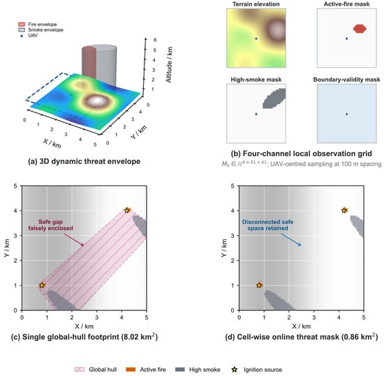
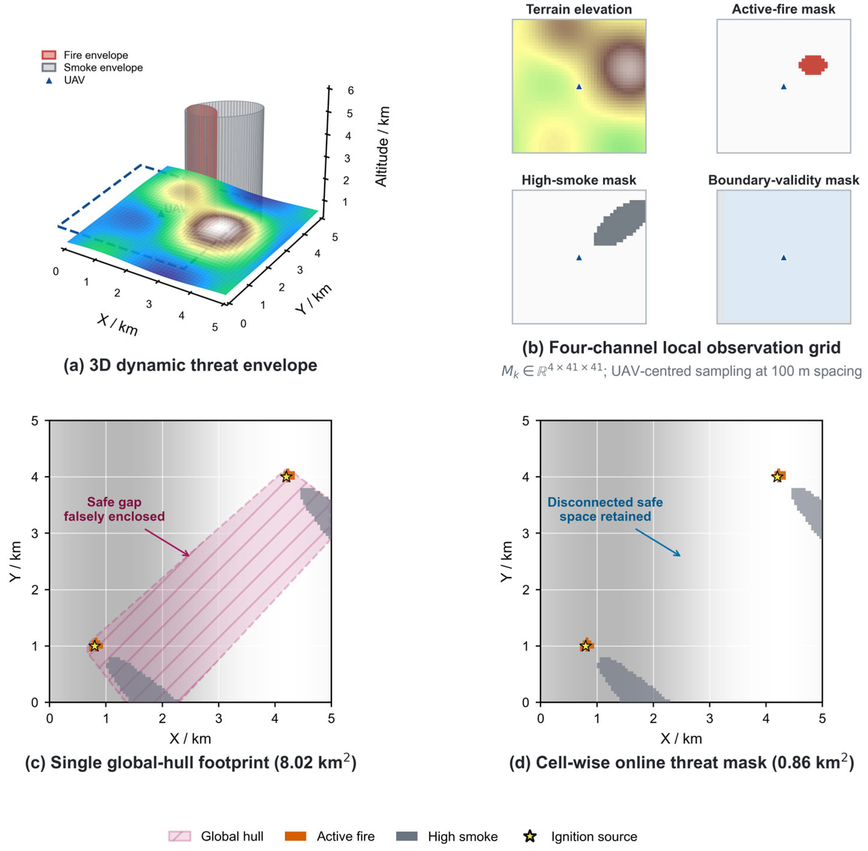
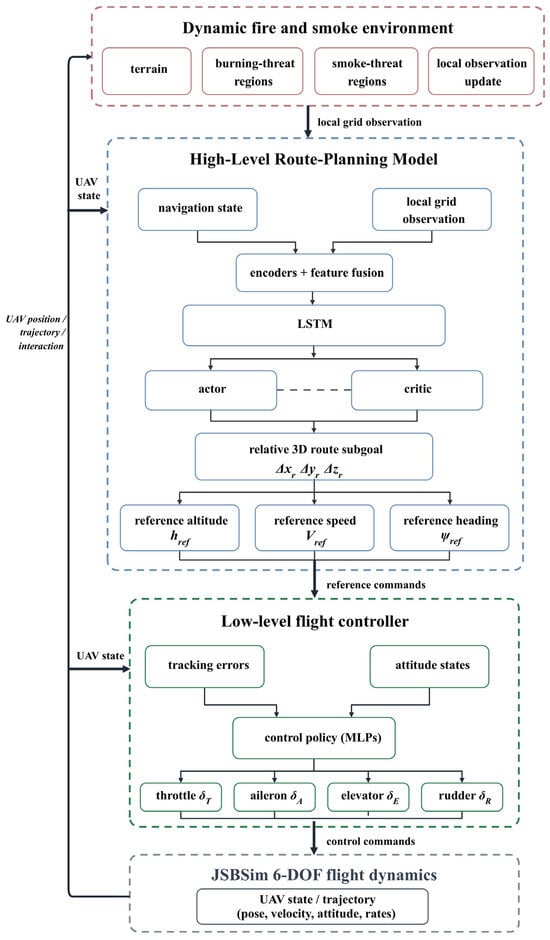
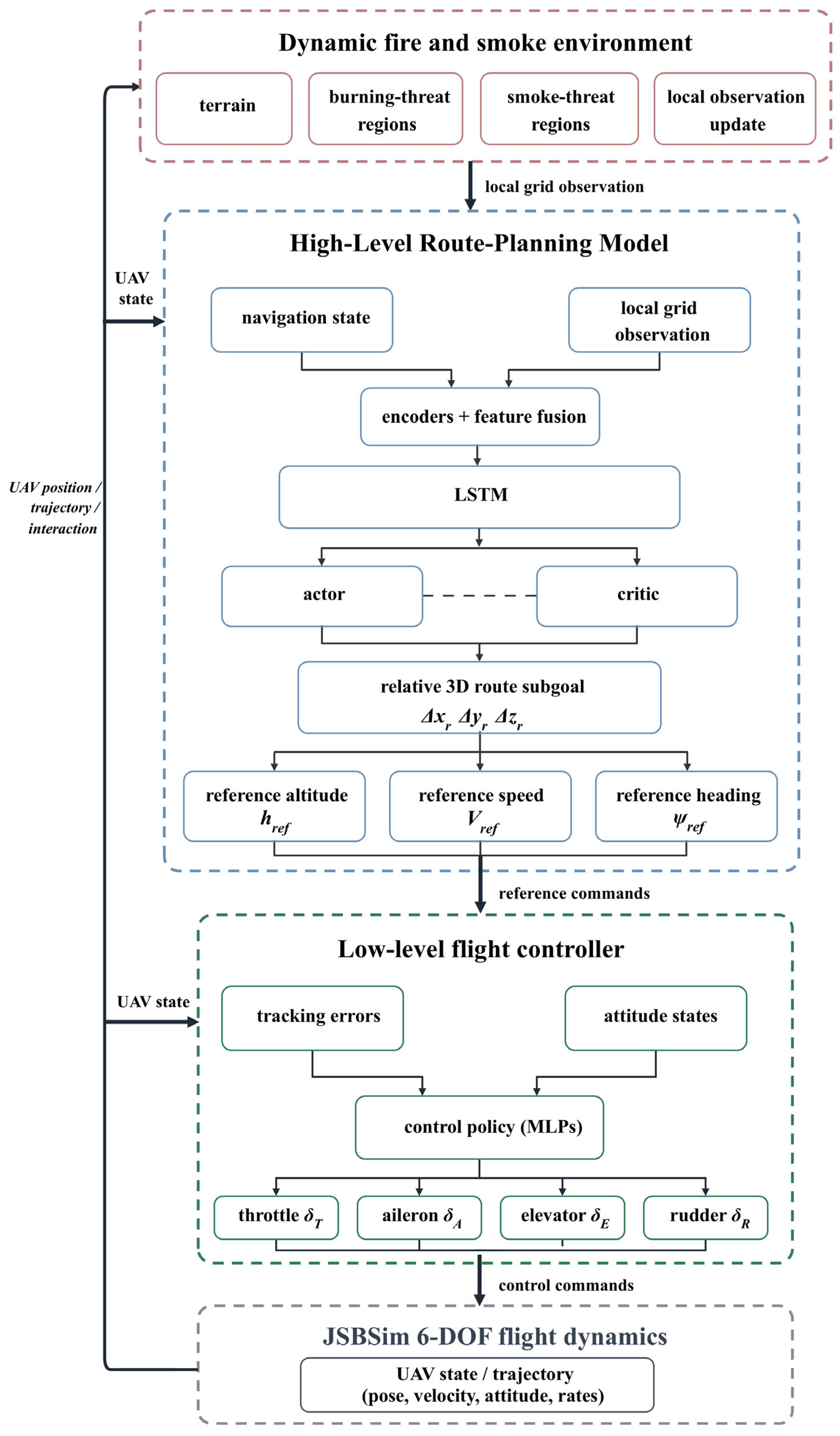
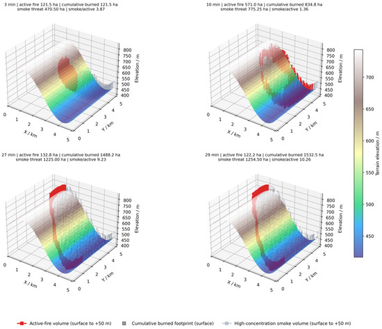
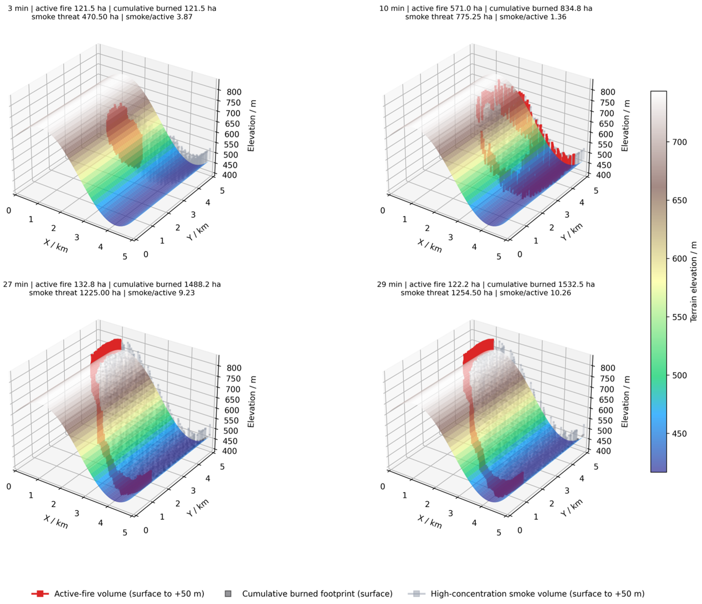
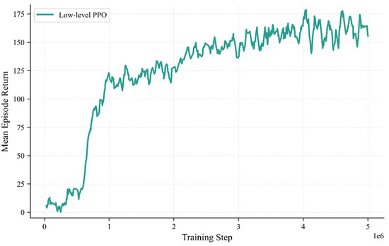
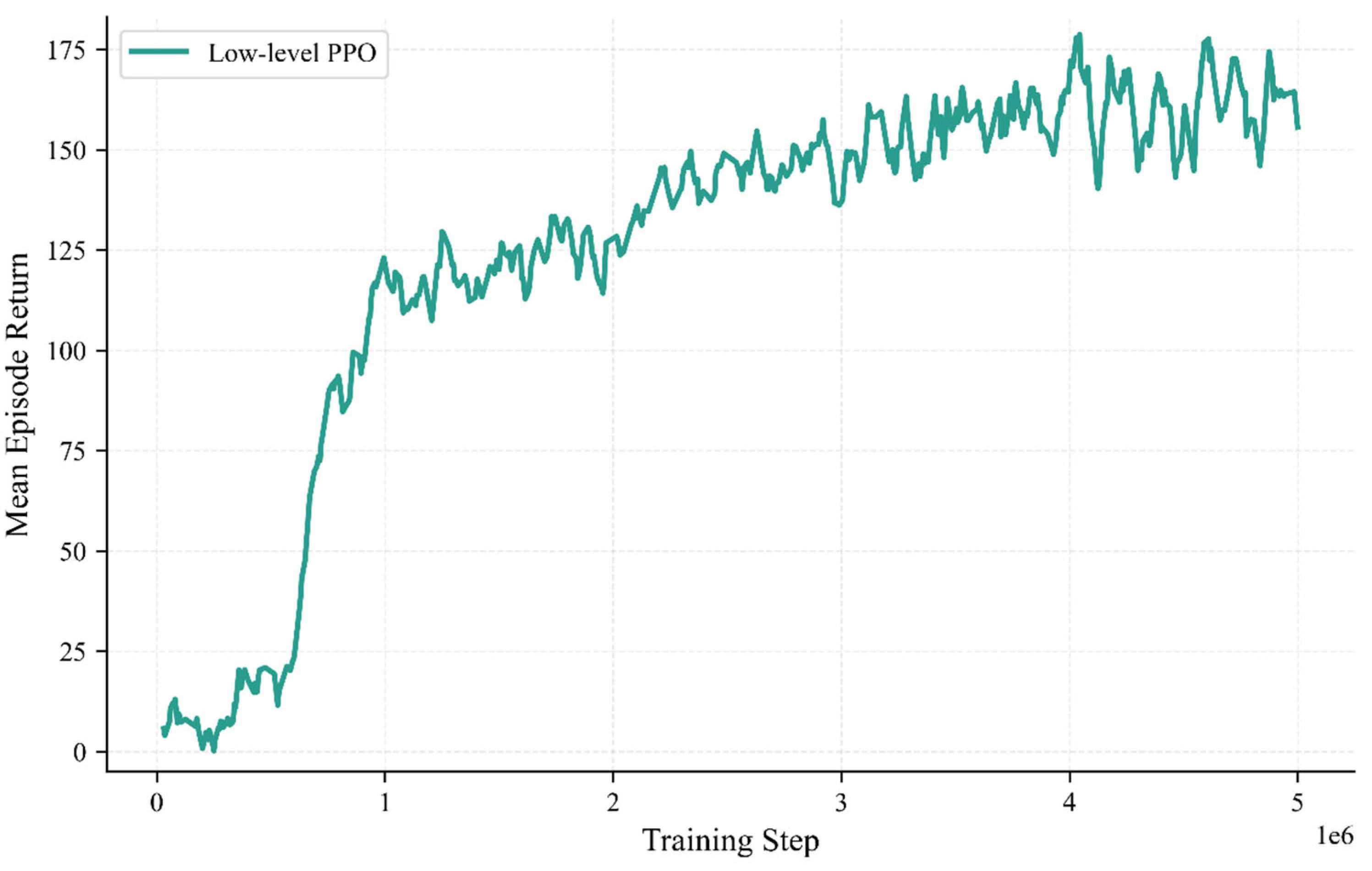
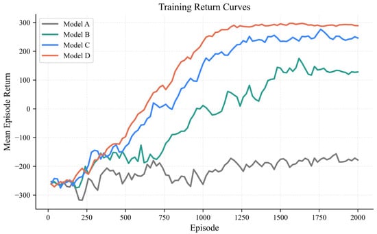
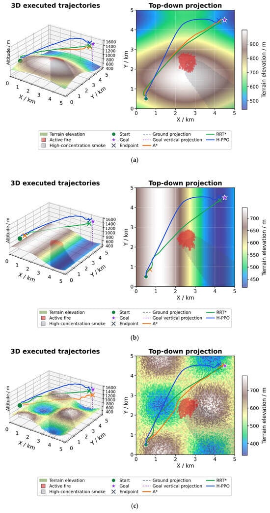
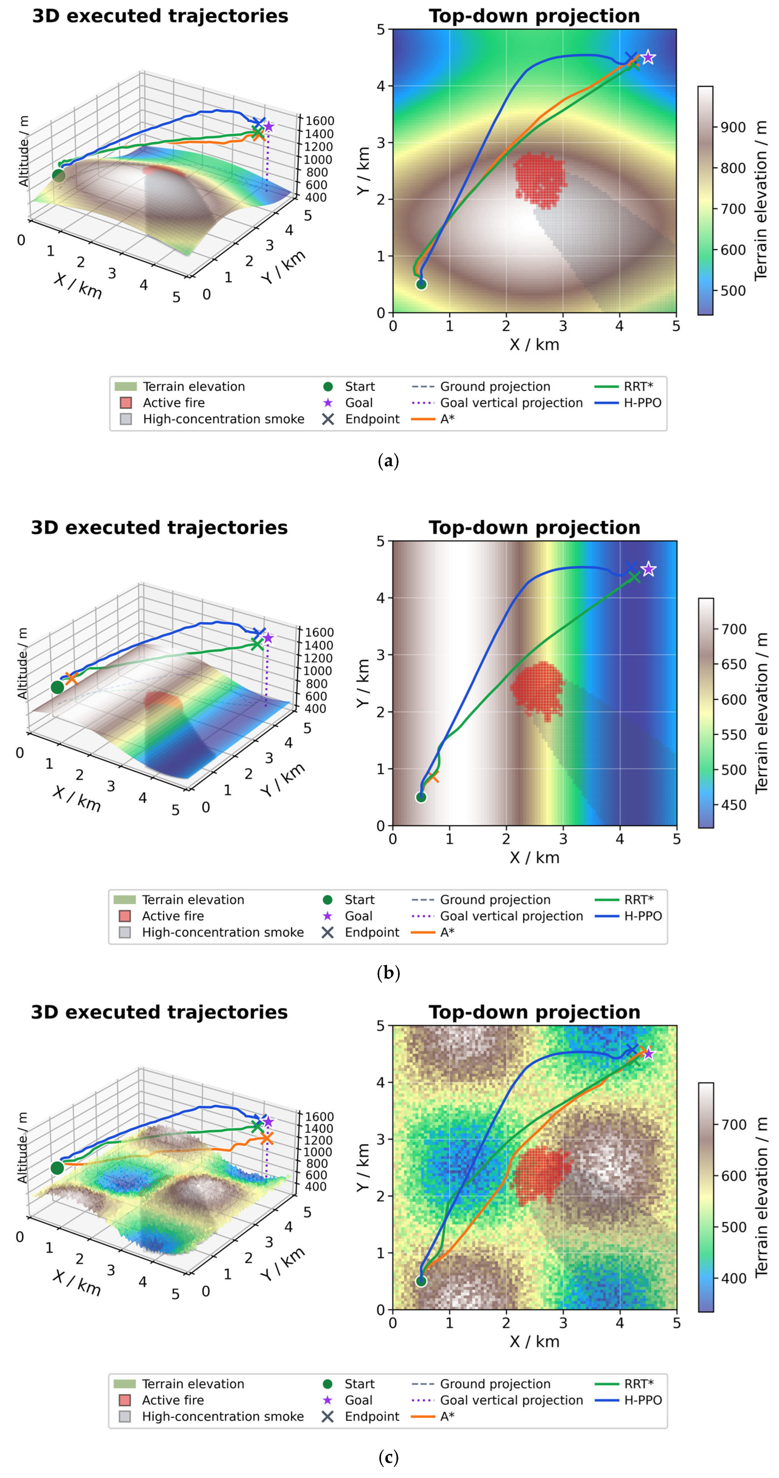
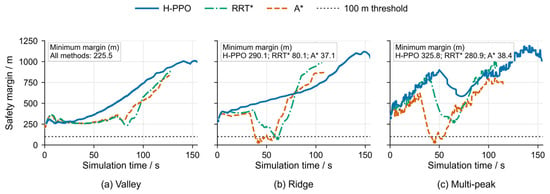
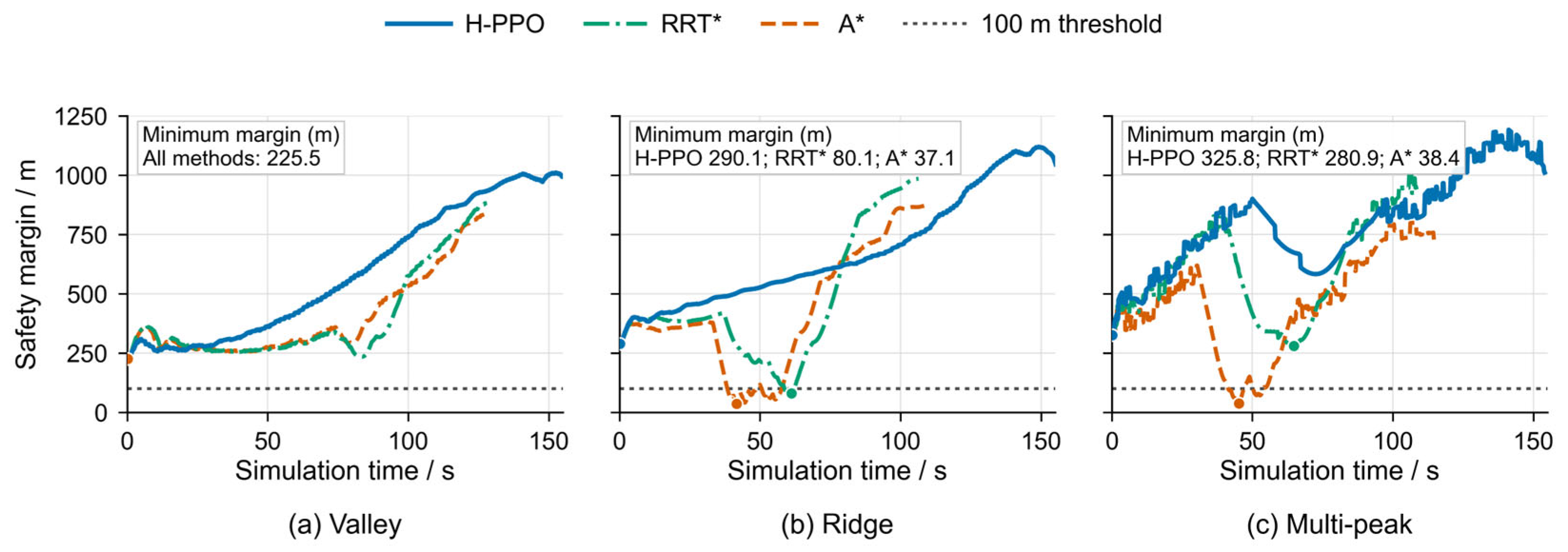
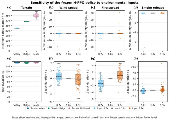
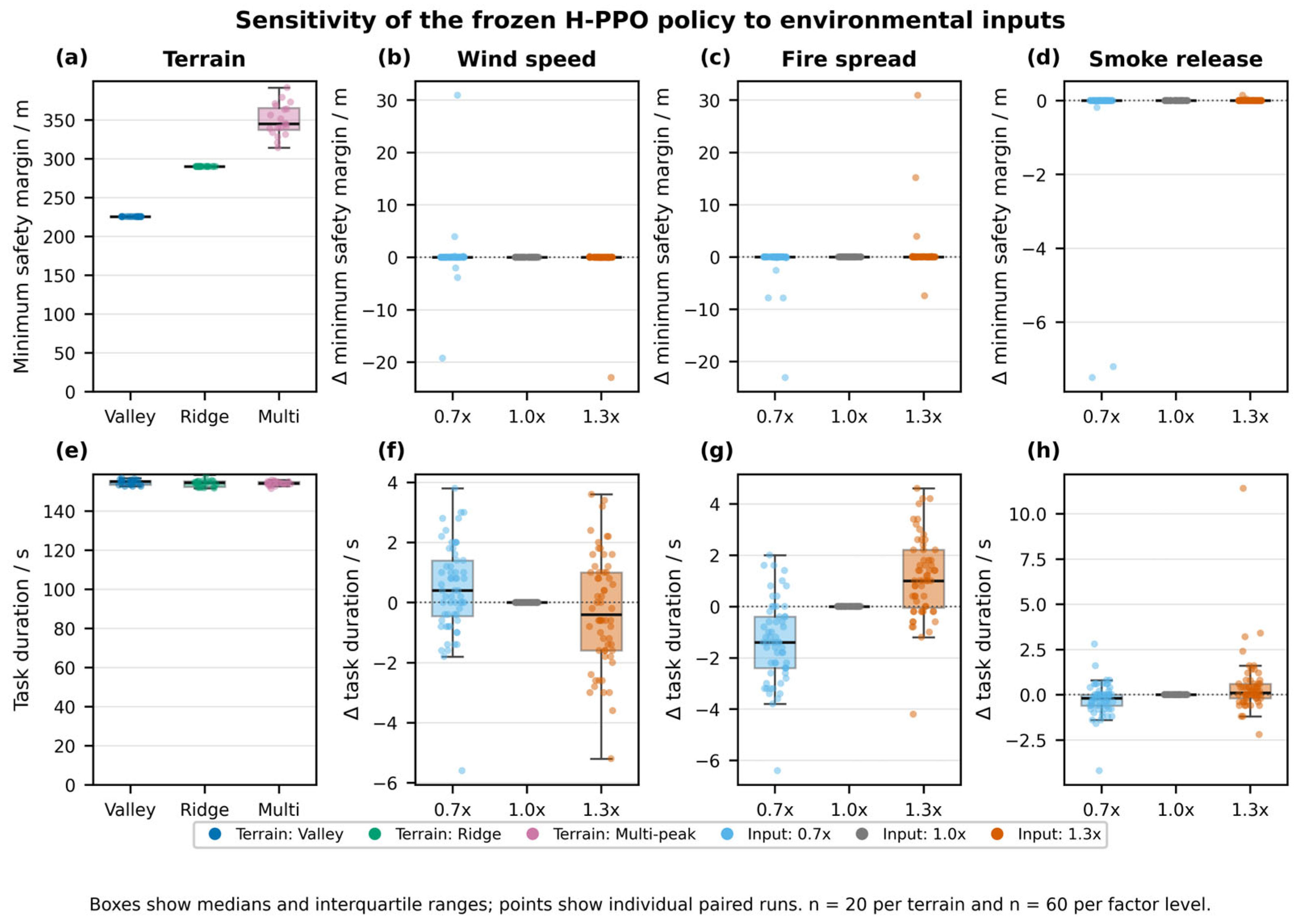

Disclaimer/Publisher’s Note: The statements, opinions and data contained in all publications are solely those of the individual author(s) and contributor(s) and not of MDPI and/or the editor(s). MDPI and/or the editor(s) disclaim responsibility for any injury to people or property resulting from any ideas, methods, instructions or products referred to in the content. |
© 2026 by the authors. Licensee MDPI, Basel, Switzerland. This article is an open access article distributed under the terms and conditions of the Creative Commons Attribution (CC BY) license.