


Highlights
What are the main findings?
- LLSOA outperforms four other swarm intelligence algorithms (DBO, GWO, PIO, PSO) in 3D urban path planning, with superior path length, smoothness, and convergence speed, while effectively handling complex waypoint constraints to bridge the gap between theory and real-world UAV missions.
- AirSim simulations with GPS/IMU noise further confirm that LLSOA-planned paths maintain stability under realistic sensor perturbations.
What are the implications of the main findings?
- LLSOA offers a robust, constraint-aware global planning solution for UAV operations in complex urban environments, where the LHS + Lévy Flight strategy significantly improves SOA performance in multi-constraint path planning.
- The ability to handle waypoint constraints and overcome sensor noise to a certain extent indicates that LLSOA has strong potential for real-world deployment.
Abstract
UAV path planning in complex urban environments faces significant challenges due to dense obstacles, narrow corridors, and stringent safety requirements. To address these issues, this paper proposes LLSOA, a modified Seagull Optimization Algorithm that integrates Latin Hypercube Sampling (LHS) for population initialization and Lévy Flight for global search. The key innovation lies in the problem-driven design: LHS ensures uniform coverage in dense urban maps, while Lévy Flight helps escape local optima. Compared with four state-of-the-art swarm intelligence algorithms (DBO, GWO, PIO, and PSO) across four urban scenarios, LLSOA achieves the best comprehensive fitness. Considering multiple constraints including path length, curvature, collision avoidance, and obstacle-avoidance logic, the trajectories generated by LLSOA show competitive overall performance, with no unsafe points recorded in the test scenarios and the best fitness values among the compared algorithms, albeit with a slight trade-off in path length. High-fidelity AirSim simulations with GPS/IMU noise further demonstrate that the planned trajectories remain within engineering acceptable limits. Compared with the noise-free baseline, the maximum trajectory deviation increases by 2.3% and the average deviation increases by 2.8% under high GPS/IMU noise. The main contributions are: (1) a problem-driven LLSOA that combines LHS and Lévy Flight, specifically tailored to dense urban environments; (2) theoretical analysis and simulation verification demonstrating its feasibility for multi-constraint path planning under the tested conditions; (3) high-fidelity (UE+AirSim) validation showing that the generated trajectories retain stability even under realistic sensor noise.
1. Introduction
When conducting flight operations in intricate environments characterized by dense urban structures, UAVs encounter multifaceted challenges including numerous obstacles, stringent public safety requirements, and the imperative to prevent collision incidents. Concurrently, given the extensive array of viable trajectories, it becomes essential to harmonize path optimization with energy-efficiency considerations to ensure mission objectives are accomplished effectively. Consequently, the trajectory planning and optimization challenge for UAVs in complex environments fundamentally represents a multi-constraint comprehensive optimization problem. The primary methodologies for addressing these challenges encompass: traditional mathematical programming techniques, swarm intelligence approaches, machine learning frameworks, hybrid algorithms, and other methodologies.
Although conventional mathematical programming approaches can ensure precise solutions for typical path-planning challenges, their efficacy diminishes when addressing more complex path-planning scenarios, typically yielding only a single solution per execution [1]. A review indicates that although the weighted sum method is the most widely used approach in military UAV path planning, its oversimplified nature may lead to the loss of critical trade-off information [2].
Cluster intelligent algorithms stand as the most widely adopted and intensively studied approach for UAV path-planning [3], exhibiting remarkable aptitude for tackling complexity and resolving multi-objective conflicts in UAV path-planning scenarios. The advantage of swarm intelligence algorithms resides in their capacity to produce multiple viable solutions for selection within a single execution, alongside their aptitude for managing nonlinear and intricate discrete environments [4,5]. The limitation is that they fall under the category of heuristic approaches, which cannot ensure the identification of global optimal solutions, and the configuration of parameters substantially affects the results [6].
The advantage of machine learning approaches is demonstrated through their remarkable adaptability, ability to operate effectively in highly dynamic and unpredictable environments, and superior real-time performance capabilities. However, these methods come with certain limitations, such as the necessity for substantial training datasets or extended interaction periods, alongside the inherent “black box” characteristic of many models, which often results in limited interpretability and challenges in comprehending the underlying decision-making mechanisms [7,8].
Hybrid algorithms can harness complementary strengths by integrating the benefits of diverse methodologies. For instance, algorithms with strong global search capabilities are employed to identify rough paths, followed by fine-tuning and obstacle avoidance through local optimization or learning approaches. The advantages of fusion algorithms lie in their powerful performance, ability to handle extremely complex real-world problems, and good robustness. However, the disadvantages include complex algorithm design, potentially high demand for computing power, and greater difficulty in parameter tuning [9].
In the practice of UAV path planning within urban environments, traditional mathematical programming approaches typically necessitate the construction of accurate mathematical models. While mathematical modeling possesses intrinsic advantages in terms of problem interpretability and result predictability, the quality of mathematical modeling is closely associated with the designer’s comprehension of the fundamental logic of the problem and professional capabilities. Accurate modeling frequently entails substantial complex data requirements and computational demands. Currently, mainstream solving methods tend to opt for machine learning approaches or fusion methods based on swarm intelligence algorithms [10,11].
Metaheuristic algorithms are a category of general swarm intelligence algorithms formulated based on intuition or experience, aiming to obtain approximate optimal solutions for complex optimization problems within an acceptable computational cost. These algorithms achieve a balance between the two mechanisms of diversified search and collective exploration. Classical metaheuristic algorithms encompass genetic algorithms (GA) and differential evolution (DE) [12]. Presently, the prevalent and relatively novel swarm intelligence algorithms include the Particle Swarm Optimization algorithm (PSO) [13], the Dung Beetle Optimization algorithm (DBO) [14], the Grey Wolf Optimization algorithm (GWO) [15], the Pigeon-Inspired Optimization algorithm (PIO) [16], and the Seagull Optimization Algorithm (SOA) [17]. At present, the development of swarm intelligence algorithms is demonstrating a tendency of dynamism and prosperity [18,19,20,21]. The metaheuristic algorithms only require designing a corresponding fitness function for comprehensive evaluation, combined with an appropriate optimization solver, making it highly suitable for solving urban environmental UAV path-planning problems [22].
Compared with machine learning algorithms, metaheuristic algorithms demonstrate superior compatibility regarding hardware resource requirements and development thresholds. Machine learning models usually demand high-performance GPUs or multiple servers for extended simulation training. Metaheuristic algorithms impose minimal hardware requirements and demonstrate low computational time costs. A standard personal computer can typically generate satisfactory results within minutes to tens of minutes, making them particularly suitable for solving problems requiring flexible deployment strategies. However, this approach demands that designers possess an in-depth understanding of the underlying logic of specific challenges. In terms of programming development, the logical framework of metaheuristic algorithms remains relatively intuitive, with code implementation and debugging complexities significantly lower compared to machine learning methodologies. Moreover, it does not rely on pre-accumulated datasets or self-generated data pools for training, offering advantages in terms of code openness, computational efficiency, and interpretability of results.
Furthermore, human expert experience and intuitive insights can be incorporated into metaheuristic algorithms. Such knowledge, often characterized by ambiguity and difficulty in quantification, can be integrated into the optimization search process by adjusting the fitness function or operational logic of the metaheuristic algorithm.
The Seagull Optimization Algorithm (SOA) was proposed by Gaurav Dhiman and Vijay Kumar in 2018 and officially published in the journal Knowledge-Based Systems in 2019. It is a newly proposed swarm intelligence optimization algorithm in recent years. The Seagull Optimization Algorithm (SOA) is an intelligently designed metaheuristic optimization algorithm characterized by simplicity in implementation and exceptional global search capabilities, with validated application value across diverse domains. To address the multi-objective optimization challenges encountered by UAVs operating in complex urban environments with dense buildings, targeted enhancements must be implemented to the original SOA framework.
It is worth noting that a complete autonomous navigation system for UAVs consists of two closely coupled components: path planning and trajectory tracking control. While the present work focuses on the planning aspect, the feasibility of a planned path ultimately depends on the capability of the low-level flight controller to accurately track the reference trajectory under external disturbances and model uncertainties.
Recent years have witnessed significant advances in UAV trajectory tracking control. Classical nonlinear methods such as backstepping sliding-mode control with disturbance compensation [23,24] and active disturbance rejection control (ADRC) have demonstrated strong robustness against external perturbations. Meanwhile, learning-based approaches have emerged as promising alternatives. Reinforcement learning (RL) and deep reinforcement learning (DRL) methods have been increasingly applied to UAV control, enabling adaptive decision-making in dynamic environments through interaction with the environment [25,26]. Multi-agent reinforcement learning (MARL) has also been explored for cooperative UAV control in scenarios requiring coordinated trajectory tracking [27]. Additionally, hybrid control strategies that integrate neural networks with classical controllers (e.g., ANN-PID) have shown improved adaptability and tracking accuracy [28].
These control methods provide the necessary foundation for executing the paths generated by planners. The integration of the proposed planning framework with such robust control strategies—whether model-based or learning-based—represents a promising direction for future work.
2. Related Work
SOA demonstrates stable search performance with minimal application parameters while balancing high-dimensional and low-dimensional optimization. This makes it ideal for solving complex multi-constraint problems. After its introduction, numerous scholars have conducted in-depth research and refinements on SOA according to the practical application requirements in their respective fields of study.
According to Pathak et al.’s analysis of 109 studies since 2019, the main directions for SOA variants are focused on hybridization, chaotic mapping, and Lévy Flights. The research fields mainly include engineering design and path planning [29]. Currently, research on SOA improvement algorithms is receiving widespread attention from researchers in related fields.
Recently, several studies have applied path-planning research using state-of-the-art SOA improvements. Chen et al. proposed LSOA, a Lévy-based SOA, which was validated on benchmark functions with a simple path-planning example [30]. Zhou et al. proposed a Tent–Lévy-based SOA for multi-UAV task allocation [18]. Huang et al. proposed an improved SOA for multi-center maintenance task allocation under resource constraints [31]. Zhang et al. proposed a multi-strategy-improved SOA integrating Lévy Flight, adaptive control factor, and elite retention for UAV 3D path planning in mountainous orchards [32].
Despite the satisfactory performance of SOA in various optimization tasks, its application to UAV 3D path planning in complex urban environments remains largely underexplored. A critical analysis of existing SOA variants reveals several limitations. For instance, the Lévy-based LSOA was primarily validated on benchmark functions with only a simple path planning example, lacking rigorous testing in realistic UAV scenarios. The Tent–Lévy-based SOA was designed for multi-UAV task allocation rather than continuous 3D path planning, and it did not consider environmental constraints such as dense obstacles or narrow corridors. Similarly, the multi-strategy-improved SOA for orchard path planning operates in open agricultural spaces, where obstacles are sparse, and constraints are less stringent compared to urban canyons. More importantly, none of these existing SOA variants have been validated in high-fidelity simulations that account for sensor noise, dynamic disturbances, or realistic flight dynamics. To fill these gaps, we propose LLSOA, which integrates Latin Hypercube Sampling (LHS) for diversity-enhanced population initialization and Lévy Flight for global search capability. The main contributions of this work are threefold:
- A problem-driven algorithm design specifically tailored to dense multiple-constraint urban environments;
- The first application of the LHS + Lévy Flight combination to UAV 3D path planning;
- Comprehensive validation in AirSim under GPS/IMU noise, demonstrating practical viability.
3. Analysis and Improvement of Seagull Optimization Algorithm
3.1. Analysis of Seagull Optimization Algorithm
Inspired by the migratory and predatory behaviors of seagulls in nature, the inventor of the Seagull Optimization Algorithm proposed a novel swarm-intelligence optimization algorithm. The fundamental idea of the Seagull Optimization Algorithm is to regard the solution space of the problem as a sea area and the objective function to be optimized as food in the sea. The initial population of the Seagull Optimization Algorithm (SOA) is regarded as seagull individuals randomly distributed in the three-dimensional space of the sea area. The algorithm achieves the solution of the objective function through two behaviors: migration and attack. Migration behavior refers to seagulls flying from a place that is currently unsuitable for survival to a place that is suitable for survival, corresponding to the global exploration ability of the algorithm. The algorithm introduces individual collision avoidance in the migration mode to expand the search range of the algorithm and improve the individuals’ ability to find the optimal position. Attack behavior simulates the attack process of seagulls on food in the area during flight, corresponding to the local exploitation ability of the algorithm, and its mathematical model can be represented as a spiral [33].
3.1.1. Migration Behavior
During the migration process, seagulls can achieve position transformation and optimization by continuously adjusting their flight angle and speed. The algorithm conducts a global search by simulating the migration behavior of seagulls. In this process, the following conditions must be met:
- Avoid collisions [33]
When the positions of seagulls change during migration, the position differences between individuals should be maintained, which ensures that the diversity of the population can be preserved. To prevent collisions between migrating seagulls, the inertia weight factor A is utilized to update the positions of seagulls.
where is the position where the search individual does not collide with other individuals;
is the location information of the current search individual;
t is the t-th iteration;
The inertia weight factor A represents the search movement behavior of the search individual in a given hunting space.
where T is the maximum number of iterations;
is used to control the frequency of A, and the value is usually 2.
The value of parameter A decreases linearly with the increase in iteration times.
- Move to the optimal position [33]
The seagulls move to the optimal position to simulate the individual optimization process. Under the control of parameter A, seagulls move to the global optimal position based on the constraint of avoiding collision. The formula is as follows:
where is the location information of the search individual after moving towards the best neighbor ;
B is a random value to balance the algorithm’s exploration and development capabilities. Its calculation method is as follows:
where rand is a random number between [0, 1].
- Optimal location migration [33]
After avoiding individual collisions during the movement process, seagulls will migrate towards the globally optimal position. In the process of multiple iterations, the overall position of the population gradually approaches the optimal solution of the algorithm, which is a continuous optimization process. The expression is as follows:
where is the distance between the search individual and the best individual.
3.1.2. Attack Behavior
The attack behavior corresponds to the local development process. By simulating the attack behavior of seagulls during predation and leveraging the historical experience in the search process, the algorithm allows seagulls to adopt a spiral motion mode of continuously adjusting the angle and speed after approaching the target position to capture prey. The description of mapping the attack behavior trajectory to three-dimensional space is as follows:
where r is the radius of the circling behavior of seagulls;
k is a random number between [0, 2π];
u and v are a pair of constants, which are used to describe the specific characterization of the circling behavior, and the values are both 1;
e is the base of natural logarithm. To sum up, the location update formula of the search individual is as follows:
where is the final position of the seagull.
After the spiral position update, each individual is further adjusted toward the global best position using a learning rate lr. This operation is applied only in the implementation to enhance convergence stability.
where MaxIter is the maximum number of iterations.
3.2. Limitations of Seagull Optimization Algorithm
3.2.1. Room for Improvement in Initial Population Generation
Generating the initial population is the first step of the Seagull Optimization Algorithm. The quality of the initial population has a decisive impact on the convergence speed, solution accuracy, and the acquisition of the global optimal solution of the algorithm. The Seagull Optimization Algorithm uses a completely random way to generate the initial population. Although such methods can ensure the complete operation of the algorithm, there are often the following potential problems [34]:
- Lack of population diversity
The lack of population diversity is closely related to the impact of the initial population quality.
On the one hand, the distribution of the randomly generated population is often uneven. In some regions, the individuals are too dense, while in other regions, they are relatively sparse. This uneven distribution easily causes the algorithm to fall into the local optimal trap, thus missing the opportunity to explore other potential optimal solution regions. If the convergence ability of the subsequent optimization algorithm is too strong, it will further accelerate the convergence process and eventually lead to premature convergence of the algorithm. On the other hand, like most swarm intelligence algorithms, the performance of SOA largely depends on the quality of the initial population. If the randomly generated initial solution is unevenly distributed or of poor quality, it will directly affect the final optimization effect and convergence speed of the algorithm.
The two factors are superimposed on each other, which makes the irrationality of the initial population distribution and the convergence characteristics of the algorithm restrict the global search ability and the stability of the optimization results.
- Lack of prediction of the optimal solution
The defect of “blind exploration” caused by simple randomness is particularly prominent in complex optimization problems. For example, in the three-dimensional path planning of UAVs, the prior knowledge such as terrain obstacle distribution, no-fly zone location, and target point orientation actually constitutes the implicit solution space constraints. If this information can be integrated into the population generation process in some form during the initialization stage, the search direction can be guided to converge in the high-quality area within the feasible region. However, the traditional random initialization method treats all solution space regions equally. It can neither distinguish high-potential regions from low-value regions nor dynamically adjust the sampling density according to the characteristics of the problem, resulting in a highly disordered exploration of the algorithm in the solution space. More importantly, when the dimension of the problem increases, the volume of the solution space expands exponentially, and the proportion of effective areas covered by random sampling decreases sharply. The “dimension disaster” effect further aggravates the sparsity of the distribution of the population on key decision variables, and the probability of the algorithm finding the global optimal solution decreases significantly. In addition, random initialization lacks an active control mechanism for the difference between individuals of the population. Multiple individuals may be highly similar or even repeated, resulting in redundant consumption of computing resources and weakening the ability of the population to promote global exploration through information sharing in the early stage of evolution. For specific types of problems, human experts can usually identify the “suboptimal solution” or an approximate solution in relative optimization and optimize it on this basis, which can significantly improve optimization efficiency. However, the population generation method that completely relies on random initialization completely ignores this part of information with guiding value, which may cause additional computational resource consumption and time waste.
3.2.2. Potential Enhancements in the Optimization Process
SOA realizes global search by simulating the migration process of seagulls and local optimization by simulating the predatory attack process of seagulls. At present, according to the default method proposed by the author, there are mainly the following problems:
It is difficult to balance the convergence speed and accuracy. In the migration process of SOA, individuals move in the direction of the optimal individual in the population, which is overly linear. Although this approach is direct, it will lead to the premature loss of population diversity. All the individuals converge to the same region, causing the remaining regions in the search space to be ignored in the early stage of the optimization process, resulting in insufficient global exploration. The linear parameter setting of the algorithm often fails to perfectly match the nonlinear optimization process of complex problems. This may lead to insufficient global exploration ability and the inability to quickly locate high-quality areas in the early stage of the algorithm. In the late stage of the algorithm, the local development ability is not refined enough, which affects the convergence accuracy and speed.
The solution accuracy is insufficient, and it is prone to falling into local optimization. In the attack behavior of SOA, the default motion trajectory of seagulls is spiral. Although such a path is conducive to local optimization, it lacks sufficient randomness during the process, preventing the algorithm from jumping out of the local optimal region and exploring other adjacent regions. Once all the individuals gather in a local optimal region, the algorithm will fall into a local optimal situation. When dealing with complex multimodal functions, such as those with multiple local optima or high-dimensional optimization problems, SOA is prone to the “premature” phenomenon, that is, it stops in a local optimal region before finding the global optimal solution, resulting in low accuracy. In complex problems, the optimal solution exists among all local extremum points. It is necessary to dynamically adjust the intensity of exploration and exploitation during the search process to find the optimal solution or a sub-optimal solution as close to the optimal one as possible. However, the original SOA does not incorporate a method for breaking out of the local optimum, making it difficult to escape the local extremum area and initiate the process of seeking a better solution.
3.3. Improvement of Seagull Optimization Algorithm
3.3.1. Improvement of Initial Population Generation
To solve the problem of insufficient population diversity, the Latin Hypercube Sampling (LHS) method is introduced to optimize the initial population generation process.
Latin Hypercube Sampling is an efficient multivariate uncertainty analysis technology, which is essentially the generalization of the Latin matrix in a multidimensional space. The core idea is to divide the interval of each variable into equal-probability sub-intervals that do not overlap, and ensure that each sub-interval is sampled only once. This hierarchical sampling method can ensure the uniform distribution across all dimensions, so as to achieve high coverage of the parameter space with a small sample size. Since the number of samples does not need to increase exponentially as the dimension increases, this method is especially suitable for high-dimensional simulation models. It can significantly reduce the sample demand, optimize computing resources, and greatly improve the simulation efficiency.
- The idea of Latin Hypercube Sampling (LHS)
The LHS method is based on the “partition balance” strategy:
Interval segmentation: For each dimension of multi-dimensional variables, the value range is divided into m sub-intervals with equal probability and no overlap. Generally, a uniform distribution is adopted, meaning that the length of each interval is the same.
Stratified sampling: First, for each dimension, the variable interval is evenly divided into n sub-intervals of the same number, and each sub-interval has the same probability. Then, a point is randomly selected from each sub-interval of each dimension. Once the sampling is completed, the sub-interval is no longer used to avoid repetition. Finally, these points are combined to form the initial sample set.
Random combination: The points independently extracted from each dimension are randomly arranged and combined into a multi-dimensional vector to form a matrix of M multi-dimensional sample points, ensuring that the sampling points on any dimension evenly cover the entire interval.
Termination condition: The sampling process strictly follows the principle of “no replacement”, and each sub-interval contributes only one sample and then stops.
- Mathematical description of Latin Hypercube Sampling
For d-dimensional space and N samples, when calculating the sampling points of each dimension j, the arrangement is randomly generated. The sampling points of each dimension j are calculated as follows:
The randomly generated arrangement represents the interval number of the i-th sample in dimension J.
The calculation formula of sampling points is as follows:
where is a random number uniformly distributed in U (0, 1). The formula ensures that the sample points fall within the specified sub-interval while preserving randomness.
- Advantages and applications of Latin Hypercube Sampling
LHS achieves better coverage of the search space with fewer samples compared to simple random sampling [35]. The advantages of using LHS to generate the initial population are as follows:
Reduce sample demand: LHS uses stratified sampling technology to evenly extract sample points in each dimension to ensure the uniformity of multidimensional spatial distribution. Compared with Monte Carlo random sampling, LHS can achieve similar or higher accuracy with a smaller sample size.
Uniform coverage: It avoids the “hole” phenomenon in the parameter space and improves the robustness of the model. The Monte Carlo method is prone to the problem of uneven sample distribution in high-dimensional space, resulting in a sharp increase in computational costs; LHS effectively improves the sampling efficiency of high-dimensional problems by independently extracting the sample points of each dimension.
At the same time, considering that most optimization algorithms lack the prediction of the obvious relative optimal solution, when initializing the population, it imitates human beings’ intuitive judgment on things and allows some individuals to directly incorporate the waypoint information instead of generating them completely randomly.
3.3.2. Improvement of Optimization Strategy
Lévy distribution was proposed by Paul Lévy, a French mathematician, in the 1920s. It refers to a random walk where the probability distribution of step size follows a heavy-tailed distribution, and there is a relatively high probability of large strides during the random walk process. The Lévy Flight strategy can help jump out of the local optimum and quickly find the global optimum. It does this by simulating the long-distance migration behavior of animals in nature and guiding particles to search in a wider range. Compared with traditional distributions, the Lévy distribution cannot have its variance defined, and it has no moments. This makes it fundamentally different from traditional distributions such as the normal distribution in terms of statistical characteristics.
It is mentioned in the document [2]: The proposed SOA starts with a randomly generated population. The search agents can update their positions with respect to the best search agent during the iteration process. A is linearly decreased from to 0.
In the original SOA, the global search process simulated by migration is linear, and the local optimization process simulated by spiral attack also lacks randomness. Usually, this searching method is prone to falling into a local optimum due to the lack of randomness. For the above reasons, Lévy Flight was introduced in the search phase.
Lévy Flight can solve these problems precisely because of its unique random walk characteristics of both short-range exploration and occasional long-distance jumping.
Lévy Flight can solve these problems precisely because of its unique random walk characteristics, which involve both short-range exploration and occasional long-distance jumps. The Lévy Flight strategy adopts a random walking strategy, which is mainly characterized by the staggered movement of short and long distances [36]. When the step size is larger, the search range is wider; when the step size is small, the local optimization ability is stronger. Its expression is as follows:
where β is a constant.
When 0 < β < 1, the algorithm will generate more large jump steps, possess strong global exploration ability, and may skip local optimal solutions;
When β ≈ 1.5, the algorithm has a relatively balanced mixture of long and short steps, making it perform well in most optimization problems;
When β approaches 2, the step-size distribution of the algorithm approaches a Gaussian distribution, indicating strong local search ability, but it is prone to getting stuck in local optima.
and are random numbers from 0 to 1.
x is the dimension of the position vector.
σ is the Mantegna formula calculated as follows:
where is the Gamma function.
In the actual implementation, the Lévy Flight perturbation is applied as an additive step to the current global best position, rather than directly multiplying the current position. The candidate solution is generated as:
where Ls = 0.1, step is the Lévy Flight step size generated by Equation (10), and Vscale applies different scaling factors to horizontal (x, y) and vertical (z) coordinates. The candidate is then clamped to the variable bounds:
Xcandidate = XGBest +Ls × step × (Ub − Lb) × Vscale,
Xnew = min(max(Xcandidate, Lb), Ub),
An experiment was designed to prove the difference between Lévy Flight and linear random movement. Specifically, in two-dimensional space, with the same number of steps (m = 1000) and the same starting point (0, 0), the Lévy Flight and linear random algorithms were run respectively. Then, the distributions of the two algorithms were compared and observed, and the key indicators were also compared.
The Lévy Flight walker exhibits a distinct pattern of occasional long-range jumps interspersed with short local movements, whereas the linear random motion remains confined within a limited region. This characteristic heavy-tailed distribution of Lévy Flight is particularly valuable for UAV path planning, where the optimization process must frequently escape local optima caused by dense obstacles and navigate across a large, complex search space. This observation provides the empirical basis for integrating Lévy Flight into the Seagull Optimization Algorithm to enhance its global search capability.
Figure 1 shows a comparison of four sets of trajectories generated by the Lévy Flight and the linear random methods. Simultaneously, the distribution and comparison of the average step size for the Lévy Flight and the linear random methods are shown for different numbers of steps: Figure 2 shows 100 steps, Figure 3 shows 500 steps, and Figure 4 shows 1000 steps. It can be seen that as the number of steps increases, the distinction between the two methods becomes increasingly apparent in the figures. These comparative data are shown in Table 1.
Figure 1.
Examples of comparison between Lévy Flight and the linear random method to generate a trajectory.
Figure 2.
Distribution and comparison of average step length and search radius of Lévy Flight and the linear random method (100 steps).
Figure 3.
Distribution and comparison of average step length and search radius of Lévy Flight and the linear random method (500 steps).
Figure 4.
Distribution and comparison of average step length and search radius of Lévy Flight and the linear random method (1000 steps).
Table 1.
Comparison of average step length and search radius of trajectory generated by Lévy Flight and the linear random method.
From the above experiments, it can be observed that, compared with the linear random method, the distribution of Lévy Flight exhibits stronger jumping ability and a wider distribution area, which effectively expands the spatial search range. The Lévy Flight method is significantly superior to the linear random method in terms of average step-size and search radius. After sufficient tests and verifications, the average step length distribution and search radius distribution of the Lévy Flight method show an obvious linear trend statistically, while the linear random method shows a more concentrated distribution. Introducing the Lévy Flight method in the optimization phase of the SOA can not only increase the probability of the algorithm jumping out of the local optimal solution but also contribute to enhancing the overall optimization ability.
Lévy Flight is incorporated into SOA to enhance its global exploration capability. The heavy-tailed step length distribution allows the search agents to occasionally make large jumps across the search space, which is particularly beneficial for escaping local optima in complex urban environments where building clusters often create numerous local minima.
3.3.3. Pseudocode of LLSOA
By combining the above LHS method and Lévy Flight method to improve the original SOA, a modified SOA with Latin Hypercube Sampling and Lévy Flight (LLSOA) is obtained. The pseudo-code is shown in Algorithm 1:
| Algorithm 1. The Pseudocode of LLSOA. |
| 1://Phase 1: Latin Hypercube Sampling Initialization 2: X ← zeros(N, dim) 3: X ← lhsdesign(N, dim) 4: fit ← zeros(N, 1) 5: unsafe ← zeros(N, 1) 6: for i = 1: N 7: [fit(i), unsafe(i), ~] ← fobj(X(i,:), opt, data) 8: if unsafe(i) > 0 9: fit(i) ← fit(i) * (1 + 0.5 * unsafe(i)) 10: end 11: end 12: [~, idx] ← sort(fit) 13: X ← X(idx,:) 14: fit ← fit(idx,:) 15: unsafe ← unsafe(idx,:) 16: GBestF ← fit(1) 17: GBestX ← X(1,:) 18: GBestUnsafe ← unsafe(1) 19: curve ← zeros(MaxIter, 1) 20: safety_records ← zeros(MaxIter, 1) 21://Phase 2: Main Iteration Loop 22: for t = 1: MaxIter 23: Pbest ← X(1,:) 24: Xnew ← zeros(N, dim) 25: for i = 1: N 26: A ← fc − t * fc/MaxIter 27: Cs ← X(i,:). * A 28: rd ← rand() 29: B ← 2 * A^2 * rd 30: Ms ← B. * (Pbest − X(i,:)) 31: Ds ← abs(Cs + Ms) 32: k ← 2 * π * rand() 33: u ← 1 34: v ← 1 35: r ← u * exp(k * v) 36: x_val ← r * cos(k) 37: y_val ← r * sin(k) 38: z_val ← r * k 39: Xnew(i,:) ← (x_val * y_val * z_val). * Ds + Pbest 40: lr ← 0.3 * (1 − t/MaxIter) 41: Xnew(i,:) ← (1 − lr) * Xnew(i,:) + lr * GBestX 42: if t < MaxIter/2 43: perturb ← 0.05 * (1 − t/MaxIter) * (rand(1, dim) − 0.5) 44: Xnew(i,:) ← Xnew(i,:) + perturb 45: end 46: end 47: for j = 1: N 48: Xnew(j,:) ← max(min(Xnew(j,:), ub), lb) 49: end 50: fit_new ← zeros(N, 1) 51: unsafe_new ← zeros(N, 1) 52: for i = 1: N 53: [fit_new(i), unsafe_new(i), ~] ← fobj(Xnew(i,:), opt, data) 54: if unsafe_new(i) > 0 55: fit_new(i) ← fit_new(i) * (1 + 0.5 * unsafe_new(i)) 56: end 57: end 58: X ← Xnew 59: fit ← fit_new 60: unsafe ← unsafe_new 61: //Update Global Best 62: for i = 1: N 63: if unsafe(i) < GBestUnsafe || (unsafe(i) == GBestUnsafe && fit(i) < GBestF) 64: GBestF ← fit(i) 65: GBestX ← X(i,:) 66: GBestUnsafe ← unsafe(i) 67: end 68: end 69: //Lévy Flight Perturbation 70: levy_beta ← 1.5 71: levy_scale ← 0.01 72: L ← Lévy(1, dim, levy_beta) 73: scale_vec ← ones(1, dim) 74: for k = 1: dim 75: if mod(k, 3) == 1 || mod(k, 3) == 2 76: scale_vec(k) ← 1.2 77: else 78: scale_vec(k) ← 0.5 79: end 80: end 81: cand ← GBestX + levy_scale * L .* (ub − lb) .* scale_vec 82: cand ← max (min(cand, ub), lb) 83: [fit_c, unsafe_c, ~] ← fobj(cand, opt, data) 84: if unsafe_c > 0 85: fit_c ← fit_c * (1 + 0.5 * unsafe_c) 86: end 87: if unsafe_c < GBestUnsafe || (unsafe_c == GBestUnsafe && fit_c < GBestF) 88: GBestF ← fit_c 89: GBestX ← cand 90: GBestUnsafe ← unsafe_c 91: end 92: [~, unsafe_idx] ← sort(unsafe) 93: X ← X(unsafe_idx, :) 94: fit ← fit(unsafe_idx, :) 95: unsafe ← unsafe(unsafe_idx, :) 96: curve(t) ← GBestF 97: safety_records(t) ← GBestUnsafe 98: end |
Although LLSOA, as a swarm intelligence algorithm, does not offer a formal convergence guarantee in the deterministic sense, its convergence behavior is supported by three mechanisms. First, the elitist strategy preserves the best-found solution at each iteration, ensuring that the search performance does not degrade. Second, the Lévy Flight operator provides occasional long jumps, which help the algorithm escape local optima and maintain global search capability. Third, the learning rate lr progressively reduces the influence of the global best solution as iterations proceed, gradually narrowing the search focus from exploration to exploitation. Together, these mechanisms drive the population toward a stable solution.
3.4. Solution Encoding and Decision Vector
In the proposed LLSOA, each individual (candidate solution) represents a complete UAV path, encoded as a decision vector consisting of the coordinates of intermediate waypoints.
The optimization problem in this paper involves two types of waypoints:
- Mandatory waypoints (fixed constraints)
These are the waypoints specified in the scenario (e.g., W1, W2, …, Wk). The UAV must pass through these points in sequence, from the start point to the target point. These waypoints are fixed constraints and are not included in the optimization variables.
- Intermediate waypoints (optimization variables)
These are the waypoints generated by the algorithm between each pair of fixed waypoints. Each individual is encoded as:
where N is the number of intermediate waypoints per segment. The dimensionality of each individual is 3 × N. Each variable is bounded within the map boundaries (xmin, xmax, ymin, ymax) and the altitude limits (zmin, zmax).
X = [x1, y1, z1, x2, y2, z2, …, xN, yN, zN],
The complete path is formed by concatenating:
where W1, W2, …, Wk are the mandatory waypoints. The fitness of each individual is evaluated based on the complete path, considering obstacle avoidance, path length, curvature, and waypoint constraints as defined in the fitness function.
Path = [Start, W1, (intermediate points), W2, (intermediate points), …, Wk, Target],
4. Simulation Scenario and Fitness Function Design
4.1. Simulation Environment Scenario
The flight path-planning experiment of the UAV in the urban building environment is designed. The experimental area is set as a 100 × 100 unit grid, and the buildings are distributed in the area with appropriate spacing. The starting point, waypoint, and target point are preset in the area. The UAV starts from the starting point according to the established sequence, passes through each waypoint in turn, and finally reaches the target point. Since this research focuses on the path-planning algorithm of the UAV, parametric modeling is carried out for the aerodynamic characteristics, handling and stability, body weight, and flight ability of the UAV. Figure 5 is an example of a flight area map.
Figure 5.
Terrain schematic diagram of UAV path planning.
4.2. Constraints for UAV Flight
It is specified that the following conditions shall be followed when solving the flight trajectory of the UAV:
- To ensure flight safety, a “safety global surface” centered at the UAV with a radius of 1 unit is set. The collision and boundary crossing of the UAV are determined through the surface of the safety globe.
- Collision with buildings must be avoided during UAV flight.
- It is forbidden for the UAV to fly out of the map boundary and enter the internal space of the building.
- The minimum flight altitude of the UAV shall not be less than 5 units.
4.3. Fitness Function Design
As the objective function of the optimization problem, the fitness function plays an important role in evaluating the quality of each solution. The fitness value directly reflects the proximity between the path and the optimal solution. The smaller the value, the better the path. When evaluating the flight trajectory of a UAV, we should not use a single index for a simple evaluation. Instead, we should comprehensively consider multi-dimensional factors and weigh them. Therefore, the fitness function should be weighted by multiple cost items, including path length cost, path curvature cost, comprehensive collision penalty, lateral offset reward, and vertical change penalty.
4.3.1. Path Length Cost
Path length is an important indicator to evaluate the quality of the route planned by the algorithm, which can effectively save the energy of the UAV and improve mission efficiency. The calculation method of path length fitness is as follows:
where is the fitness to evaluate the path cost;
is the total path of planning completion;
is the path length component between each sampling point;
is the path length weight, which is set to 0.2 in this experiment.
4.3.2. Path Curvature Cost
When the UAV is flying, excessive-angle turns and unnecessary turns should be avoided. Large-angle turning may not meet the dynamic limits of the UAV. Too many turns may lead to an increase in unnecessary path length, energy consumption, and flight time. The path curvature cost is obtained by calculating the sum of the squares of the tangent angles between adjacent path segments. Each path point is used to evaluate the smoothness of the path. The fitness function of path curvature calculates the radian of the angle between the direction vectors before and after, and accumulates the square of the angle. The calculation method of curvature cost is as follows:
where is the curvature cost equivalent;
n is the number of waypoints;
is the tangent angle.
The curvature fitness function is expressed as:
where is the curvature cost weight, which is set to 0.5 in this experiment.
4.3.3. Comprehensive Collision Punishment
The determination of collision and safety distance is an important aspect, including the determination of the UAV flying below the constrained altitude. This directly affects the feasibility of the route and is assigned a high weight. In the simulation environment, the safe distance of the UAV is defined as a “safety global surface” with a radius of 1 unit length. Collisions between the UAV and buildings, exceeding the safe flight altitude, and exceeding the map boundary are comprehensively incorporated into the comprehensive collision penalty.
Let the fitness function of the comprehensive collision penalty be , the radius of the safety globe be , the distance from the UAV to the building surface or the minimum flight altitude plane be , and the penetration depth be when the UAV is below the building surface or the minimum flight altitude plane. The comprehensive collision penalty takes into account the relative relationship between the UAV and the building or the minimum allowable flight altitude plane, and the calculation method of the comprehensive collision fitness function is as follows:
The UAV safety globe is located outside the building or above a safe-height plane with sufficient distance: ;
The UAV safety globe is located outside the building or above the safe-height plane, but the distance is not enough: ;
The UAV safety globe is located inside or under the safe altitude plane but not completely submerged in the building: ;
If the UAV is inside the building or under the safe-height plane, additional punishment will be imposed: ;
If the UAV exceeds the map boundary, it will be severely punished: .
4.3.4. Obstacle-Avoidance Logic Design
In terms of the choice of obstacle-avoidance logic, in the scenario discussed in this paper, buildings are regarded as the main obstacles, and the detour mode of the UAV can be divided into two types: ascending first and then descending, or lateral detour. The horizontal detour is preferred in the design for the following reasons:
From a flight safety perspective, for taller buildings, it is necessary to climb higher to avoid obstacles, which may lead to a more complex wind-shear environment and potential safety hazards. At the same time, the excessive accumulation of gravitational potential energy will cause more serious damage in the event of a UAV crash in the urban environment. Therefore, in actual flight, it is more advisable to maintain a relatively low safe altitude and try to avoid ascending operations. The lower limit of UAV flight altitude is also specified in the simulation scene.
Comprehensive analysis from the perspective of energy consumption: for taller buildings, the energy consumption of the transverse detour path is usually lower than that of the way of ascending first and then descending. This is because during the ascent and descent of the UAV, in addition to the basic energy consumption required to maintain level flight, the energy consumption per unit time also needs to overcome the potential energy change caused by ascent and descent, so the energy consumption is often greater. If the area is dominated by low-rise buildings, the energy consumption difference between the two paths may be small. But for high-rise buildings, this energy consumption difference will be more significant.
Therefore, the design fitness function encourages the UAV to bypass obstacles horizontally rather than by frequent ups and downs. At the same time, in order to minimize unnecessary vertical fluctuations and make flight more stable, the program focuses on optimizing horizontal obstacle-avoidance paths. All comparison methods used in subsequent experiments employed the same fitness function to ensure consistency in the computational conditions under the same scenario and constraints. Based on the above discussion, the final form of the fitness function is:
5. Experimental Verification
5.1. Experiment Environment
The experiment environment adopts the personal notebook computer Acer Predator PHN16-71; the detailed configuration includes:
- CPU: 13th Gen Intel(R) Core(TM) i9-13900HX 2.20 GHz;
- RAM: 64.0 GB;
- GPU: Intel(R) UHD Graphics and NVIDIA GeForce RTX 4060 Laptop GPU;
- Disk Drive: NVMe Micron 3400;
- Software Simulation Environment: Unreal Engine 4.27.2, AirSim 1.81, Matlab 2024b.
5.2. Simulation Experiments
5.2.1. Ablation Experiment
In order to rigorously verify the improvement effect of LLSOA, ablation research is essential. The original SOA, while demonstrating competent global search capabilities, suffers from two inherent limitations when applied to UAV path planning in complex environments. First, its random population initialization often results in uneven spatial coverage of initial solutions, potentially overlooking promising regions of the search space. Second, its step-size update mechanism during the optimization phase lacks adaptive perturbation capacity, making the algorithm susceptible to premature convergence in local optima when navigating obstacle-dense environments.
The LHS and Lévy Flight strategies address these limitations from distinct yet potentially complementary perspectives. LHS enhances the diversity and uniformity of the initial population distribution, thereby improving the algorithm’s exploration foundation. Lévy Flight introduces a heavy-tailed step-size distribution during optimization, enabling the search agent to occasionally perform long jumps that facilitate escape from local basins of attraction. However, the individual and interactive contributions of these two mechanisms to the overall algorithmic performance cannot be assumed a priori. Specifically, it remains unclear whether the performance gain originates primarily from the improved initialization, the enhanced search dynamics, or their synergistic coupling.
The ablation study systematically disentangles the individual contributions of the two enhancement modules by comparing four configurations: the complete LLSOA (LHS–Lévy-based SOA), two single-improvement variants (LHS-based SOA and Lévy-based SOA), and the baseline SOA. To assess the statistical significance of the observed differences, we applied the Friedman test to the fitness values, computation time, number of unsafe points, and path lengths obtained from 30 independent runs of each configuration. Among these metrics, fitness value serves as the primary criterion for performance evaluation, as it integrates all constraints and weighting factors into a single scalar representing the overall optimization outcome. The remaining metrics are reported as supplementary indicators to provide additional insight into the trade-offs between safety, efficiency, and computational cost. In this context, an “unsafe point” refers to a point where, although the drone has not collided with an obstacle, its distance from the obstacle is less than the safety globe .
In the ablation experiment, 15 building scenes were selected. The scene is set with a starting point, a target point, and different waypoints. The UAV needs to start from the starting point, pass through all waypoints in sequence, and finally reach the target point. The design of constraints and fitness functions has been described above. All algorithms were configured with a population size of 40, a maximum of 200 iterations, and 30 independent runs per scenario. The results of each algorithm after 200 iterations are compared. The scenario includes:
Starting point coordinates: (95, 5, 5);
Coordinates of waypoints: (79, 33, 8), (55, 47, 10), (32, 38, 10), (13, 75, 6);
Target point coordinates: (5, 93, 5).
The path-planning and optimization effects of SOA, LHS-based SOA, Lévy-based SOA, and LLSOA were compared under the same conditions. Figure 6 presents a representative example of the paths generated by the four algorithms in one of the test scenarios. The corresponding quantitative results are summarized in Table 2 and Table 3.
Figure 6.
Example of planning results for SOA, LHS-based SOA, Lévy-based SOA, and LLSOA across 15 building scenarios.
Table 2.
Comparison results of four algorithms across four evaluation metrics (SOA, LHS-based SOA, Lévy-based SOA, and LLSOA, each for 30 independent runs).
Table 3.
Comparison of average ranks from Friedman tests for four algorithms across four evaluation metrics (SOA, LHS-based SOA, Lévy-based SOA, and LLSOA, each for 30 independent runs).
- The result of the Friedman test
A Friedman test was performed on the results of the ablation experiments (SOA, LHS-based SOA, Lévy-based SOA, and LLSOA), yielding the following results:
The Friedman test results confirm that the four algorithm variants exhibit statistically significant differences in fitness (p < 0.001), unsafe points (p < 0.001), time (p < 0.001), and path length (p = 0.024). LLSOA achieves the best mean rank in fitness (1.30), demonstrating that both the LHS and Lévy Flight modules contribute effectively to the overall performance improvement. The slightly longer path length of LLSOA is a reasonable compromise for ensuring collision-free navigation in complex urban environments. At the same time, as an offline planning algorithm, LLSOA has a computation time that falls within an acceptable range.
5.2.2. Comparative Experiment
To comprehensively evaluate the proposed LLSOA, we compare it against four representative swarm intelligence algorithms: DBO, GWO, PIO, and PSO. These algorithms are selected for their distinct optimization paradigms: DBO exhibits competitive global search through rolling and dancing behaviors; GWO leverages hierarchical social hierarchy and encircling mechanisms for strong convergence; PIO incorporates map-and-compass and landmark operators for multi-modal optimization; and PSO, as a classical velocity-position framework, has been widely adopted in early UAV trajectory optimization studies. Their proven effectiveness in path-planning problems justifies their inclusion as benchmarks.
To evaluate the statistical significance of the performance differences among the five algorithms, we adopted a two-stage statistical testing procedure.
First, the Friedman test was applied to detect overall performance differences among the five algorithms for each evaluation metric. The Friedman test is a non-parametric alternative to repeated-measures ANOVA, which does not assume normality and is robust against outliers—particularly suitable for metaheuristic algorithm comparisons. A significant Friedman test result (p < 0.05) indicates that at least one algorithm differs from the others in terms of the tested metric.
Second, when the Friedman test confirmed a significant overall difference, we conducted pairwise Wilcoxon signed-rank tests between LLSOA and each of the four competing algorithms (DBO, GWO, PIO, and PSO). The Wilcoxon signed-rank test is a non-parametric paired difference test that evaluates whether the performance of LLSOA is statistically superior to that of each competitor.
All statistical tests were performed at a significance level of α = 0.05 using 30 independent runs for each algorithm on every test scenario. Since the fitness value integrates all constraints and weighting factors into a single scalar, it serves as the primary criterion for performance comparison. The remaining metrics are reported as supplementary evidence to provide deeper insight into the trade-offs between safety, efficiency, and computational cost.
To ensure fairness, each algorithm adopts a unified environmental setting, constraint-processing mechanism, and fitness function definition. All competing algorithms were configured with their default parameters as recommended in their respective original references. No additional tuning was performed for any algorithm. The random seed was shuffled for each of the 30 independent runs to ensure statistical independence. All algorithms were configured with a population size of 40, a maximum of 200 iterations, and 30 independent runs per scenario. The UAV flight environment included 15 high-rise buildings distributed across the map, consistent with the scenarios and constraints of the previous ablation tests. Figure 7 presents a representative example of the paths generated by the five algorithms in one of the test scenarios. The corresponding quantitative results are summarized in Table 4 and Table 5.
Figure 7.
Example of planning results for DBO, GWO, PIO, PSO, and LLSOA across 15 building scenarios.
Table 4.
Comparison results of five algorithms across four evaluation metrics (DBO, GWO, PIO, PSO, and LLSOA, each for 30 independent runs).
Table 5.
Comparison of average ranks from Friedman tests for five algorithms across four evaluation metrics (DBO, GWO, PIO, PSO, and LLSOA, each for 30 independent runs).
- The result of the Friedman test
A Friedman test was performed on the results of the ablation experiments (DBO, GWO, PIO, PSO, and LLSOA), yielding the following results:
The results of the Friedman test on the experimental data show that the p-values for all four metrics are <0.001, indicating highly significant differences among the five algorithms. LLSOA ranks first in fitness (mean rank: 1.13), unsafe points (mean rank: 1.00), and computation time (mean rank: 1.53). LLSOA ranks last in path length (mean rank: 4.10), which is an acceptable trade-off for ensuring safety.
- The result of Wilcoxon signed-rank tests
To further verify the statistical significance of performance differences between LLSOA and the four comparison algorithms (DBO, GWO, PSO, and PIO), Wilcoxon signed-rank tests were conducted under the current experimental conditions and fitness function design. Four evaluation metrics were considered: fitness value, unsafe points, path length, and computation time. The significance level was set at α = 0.05, and the Bonferroni correction was applied for multiple comparison adjustments. The test results are summarized in Table 6.
Table 6.
Summary of Wilcoxon signed-rank test results (Z-values, LLSOA compared with DBO, GWO, PIO, and PSO).
As shown in Table 7, for the fitness metric, LLSOA achieves significant superiority over all four comparison algorithms (p < 0.05). Specifically, the Z-value for LLSOA vs. DBO is 2.44 (p = 0.0148), while the Z-values for LLSOA vs. GWO, PSO, and PIO are all 4.78 (p = 0.000002). These results demonstrate that LLSOA significantly outperforms all comparison algorithms in terms of solution accuracy, with particularly pronounced advantages over GWO, PSO, and PIO.
For the unsafe points metric, LLSOA achieves highly significant superiority over all comparison algorithms (p < 0.001), with Z-values ranging from 4.8 (vs. PIO) to 5.15 (vs. DBO and PSO). Notably, the Z-values for LLSOA vs. DBO and LLSOA vs. PSO both reach 5.15 (p ≈ 0), representing the most significant differences across all tests. This strongly indicates that LLSOA exhibits better robustness in constraint handling, effectively avoiding the generation of infeasible solutions.
For the path length metric, the results show a divergence: LLSOA significantly outperforms PSO (Z = 4.33, p = 0.000015) and PIO (Z = 3.88, p = 0.000106), achieving a clean sweep across all four metrics against these two algorithms. However, DBO (Z = −1.98, p = 0.0472) and GWO (Z = −4.04, p = 0.000053) significantly outperform LLSOA on this metric, indicating that these two algorithms are capable of finding geometrically shorter paths. Nevertheless, it must be emphasized that, when interpreted in conjunction with the fitness and unsafe points results, the “advantage” of DBO and GWO in path length is achieved at the cost of severely degraded solution accuracy and massive constraint violations (unsafe points significantly inferior to LLSOA). Therefore, this advantage has limited practical value in real-world engineering applications.
For the computation time metric, LLSOA exhibits highly significant computational efficiency advantages over all four algorithms (p < 0.001), with Z-values ranging from 3.55 (vs. PIO) to 4.62 (vs. PSO). This indicates that LLSOA possesses a clear advantage in convergence speed.
In summary, the Wilcoxon signed-rank test results fully confirm the comprehensive superiority of LLSOA across the three core metrics: fitness, unsafe points, and computation time. Although DBO and GWO show slightly better performance on path length, this comes at the expense of substantially poorer solution accuracy and a large number of infeasible solutions. Overall, LLSOA demonstrates the most balanced and optimal comprehensive performance across all evaluation dimensions.
5.2.3. Generalization Experiment
To evaluate the generalization capability of the proposed LLSOA under different environmental conditions, we conducted additional tests on two urban scenarios with varying obstacle densities and building configurations. Unlike the comparative and ablation studies, which focused on algorithm performance relative to other methods, this experiment aims to assess whether LLSOA can consistently generate feasible paths across diverse settings.
For each scenario, LLSOA was independently run 10 times. The evaluation metrics include: (1) success rate—the proportion of runs that produced a collision-free path; (2) fitness value—reported as mean ± standard deviation; and (3) path length—reported as mean ± standard deviation. Typical 3D trajectories are also visualized for qualitative assessment.
- Generalization Experiment 1: 10 buildings
In this experiment, 10 scenes of buildings were selected, including:
Starting point coordinates: (7, 25, 5);
Coordinates of waypoints: (33, 49, 10), (54, 39, 15), (55, 61, 20), (76, 81, 18);
End coordinates: (99, 83, 5).
Figure 8 shows an example of a trajectory generated by LLSOA under the scenario.
Figure 8.
Example of planning results for LLSOA across 10 building scenarios.
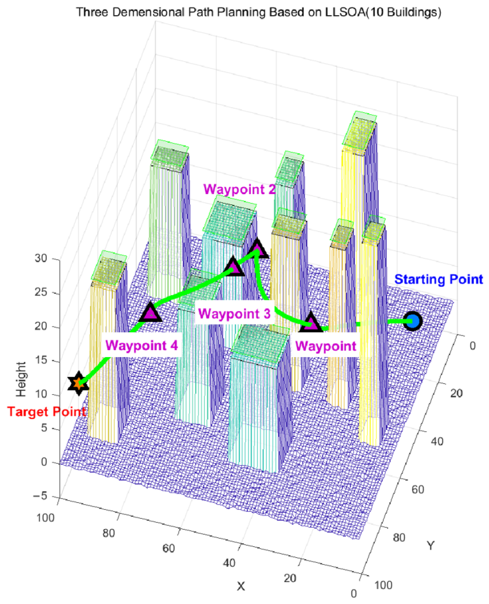
The experiment is repeated 10 times under identical conditions to assess the generalization ability of LLSOA. The key performance metrics—success rate, fitness, unsafe points, and path length—are recorded. The experimental results are summarized in Table 7.
Table 7.
Generalization experiment results for the 10-buildings scenario (10 independent runs).
- Generalization Experiment 2: 12 buildings
In this experiment, 12 scenes of buildings were selected, including:
Starting point coordinates: (1, 1, 5);
Coordinates of waypoints: (25, 34, 15), (40, 56, 20), (50, 40, 25), (83, 70, 14);
End coordinates: (100, 100, 10).
Figure 9 shows an example trajectory generated by LLSOA in this scenario.
Figure 9.
Example of planning results for LLSOA across 12 building scenarios.
The experiment is repeated 10 times under identical conditions to assess the generalization ability of LLSOA. The key performance metrics—success rate, fitness, unsafe points, and path length—are recorded. The experimental results are summarized in Table 8.
Table 8.
Generalization experiment results for the 12-buildings scenario (12 independent runs).
These results affirm the reliability and practical applicability of LLSOA for complex path-planning problems. It retains excellent planning capabilities even when transferred to other scenarios.
5.3. High-Fidelity Simulation Validation
LLSOA is an offline planning strategy. In this strategy, the algorithm pre-plans the flight path for the drone, and the drone then follows this path during flight. To verify the feasibility of this method, experiments typically need to be conducted in real urban environments to obtain conclusions with sufficient reliability. At present, our simulation utilizes Unreal Engine to create a simulated physical environment consisting of 12 buildings, which was chosen for its highly recognized physics simulation capabilities within the industry. Figure 10 is an example of an established 3D simulation scenario.
Figure 10.
Example of an established 3D simulation scenario.
This study utilizes the built-in quadcopter drone simulation model of AirSim, enabling the drone to trace the pre-planned path of the LLSOA throughout the simulation scenarios. To verify the robustness of this method, different levels of noise were introduced during the simulation. Multiple sets of repeated experiments were conducted, and the experimental results under different conditions were compared and analyzed. Figure 11 shows a flight example of UAV in 3D map. For the complete 3D environmental simulation video, see the attached Supplementary Materials.
Figure 11.
Flight example of UAV in 3D map.
This experiment directly utilizes the built-in drone model and flight control controller of AirSim. It simulates uncertain factors by adjusting the error level and sensor noise parameters in the controller settings. The comparison results of flight trajectories in a 3D high-fidelity simulation environment with those calculated by LLSOA are shown in Table 9.
Table 9.
Comparison of high-fidelity 3D simulation trajectories with deviations from LLSOA-generated trajectories.
6. Analysis and Conclusions
6.1. Analysis of Ablation Experiment
By comparing the ablation results across three urban building scenes of varying complexity, the following conclusions are drawn:
LHS alone negatively affects SOA performance (mean rank: 3.4 in fitness, 3.6 in unsafe points). Although LHS provides a more uniform initial population distribution and covers a wider solution space, the limited population size results in fewer seeds per unit space. Without sufficient long-range exploration capability, these seeds may not be effectively utilized during SOA optimization, ultimately degrading overall performance.
Lévy Flight alone substantially improves SOA performance (mean rank: 1.97 in fitness, 1.55 in unsafe points). The heavy-tail step-size characteristic enhances the local escape ability and global exploration capacity of seagull individuals, substantially improving performance even without modifying the initial population distribution.
When combined, LHS and Lévy Flight exhibit positive synergistic effects. LLSOA achieves the best overall performance (mean rank: 1.30 in fitness, 1.48 in unsafe points, 1.90 in path length). LHS provides a wider coverage of initial search starting points, while Lévy Flight effectively utilizes these points for deep exploration and local optima escape. The macro-level uniform layout of LHS complements the micro-level strong perturbations of Lévy Flight, generating synergistic benefits.
LHS serves a foreshadowing role—it does not directly deliver immediate advantages but creates favorable initial conditions for Lévy Flight. The performance enhancement of Lévy Flight demonstrates robustness, remaining effective regardless of LHS integration. The contribution of LHS is conditional, only manifesting positive effects when paired with Lévy Flight. Therefore, Lévy Flight should be regarded as the core improvement module, while LHS functions as an auxiliary enhancement module.
These findings explain why LHS-based SOA underperforms compared to SOA in ablation experiments, while the incorporation of Lévy Flight leads to substantial performance improvement, and their combination yields the best overall results.
It should be noted that the large mean fitness value (11,259,255.29) and standard deviation (42,926,172.76) of LLSOA in Table 3 are driven by two outlier runs (fitness values of 157,745,385 and 179,879,236), both caused by collision penalties. In the remaining 28 out of 30 runs (93.3%), LLSOA consistently achieved fitness values below 113, with the majority falling between 80 and 90. This indicates that LLSOA converges reliably in the vast majority of runs, while the outliers reflect the safety-first penalty mechanism.
6.2. Analysis of Comparative Experiment
By comparing the experimental results of LLSOA with DBO, GWO, PIO, and PSO algorithms in the urban building scenario, the following conclusions are drawn:
LLSOA achieves the best fitness values among all competing algorithms. This result validates that the synergistic combination of LHS initialization and Lévy Flight optimization effectively enhances the quality of path-planning in complex obstacle environments. When comparing multiple algorithms, including hierarchical-based GWO, behavior-specialized DBO and PIO, as well as the velocity-position update framework PSO, LLSOA achieved the lowest fitness values under identical conditions. The results indicate that LLSOA delivers competitive and balanced path-planning outcomes among the compared methods. As discussed in Section 6.1, the large mean fitness value of LLSOA in Table 5 is due to two outlier runs caused by collision penalties; the remaining 28 runs achieved stable fitness values below 113.
In contrast, although some comparison algorithms are outstanding in some subdivision indicators, such as path length, there are non-zero values in the number of unsafe points, which means that their planned path may face the risk of collision or execute infeasible maneuver instructions during actual flight, which is unacceptable in real-world UAV operations.
In terms of path length, the path generated by LLSOA is feasible but not necessarily the shortest. This is because, in the fitness function design, the algorithm assigns a high weight to indicators such as safety and smoothness. It ensures zero-collision and zero-rise maneuvers as a hard constraint at the expense of a slightly longer path, which meets the actual engineering needs.
In terms of calculation time, for most non-real-time tasks, such as off-line planning before flight, the computation time is acceptable, especially when considering safety and quality.
6.3. Analysis of the Generalization Experiment
The generalization capability of LLSOA is evaluated through 10-building and 12-building scenarios with complex obstacle configurations. Experimental results demonstrate that LLSOA achieves a 100% success rate across every 10 independent runs, with zero unsafe points, attesting to its high constraint-handling reliability. The algorithm consistently produces high-quality solutions with outstanding stability. Notably, the exceptionally low standard deviations across all metrics indicate that LLSOA’s performance is reproducible across independent runs—a critical attribute for practical deployment in safety-critical applications such as autonomous navigation and robotic path planning.
These findings substantiate three critical attributes of LLSOA: (I) reliability—it consistently finds feasible paths without violating constraints; (II) reproducibility—its performance is not contingent on random chance or fortunate initialization; and (III) generalizability—its advantages persist under substantially different environmental configurations. Collectively, these characteristics position LLSOA as a practical optimization tool, particularly suited for applications where safety, consistency, and predictable behavior are paramount.
6.4. Analysis of the High-Fidelity Simulation Verification
Although this high-fidelity experiment employed AirSim’s default drone model and flight control system, our tests with varying levels of sensor noise demonstrated that flight trajectory deviations remained within acceptable limits. Even under high-noise conditions, tracking errors showed no significant amplification, and the overall trajectory maintained satisfactory accuracy without occurrences of aircraft loss of control, trajectory divergence, or collisions with structures.
It is important to clarify that the robustness demonstrated in the AirSim experiments primarily reflects the trajectory-tracking controller’s ability to follow the LLSOA-planned path under sensor noise, rather than the robustness of the optimization algorithm itself. The path-planning algorithm, LLSOA, generates a static reference trajectory offline; actual tracking under noise is handled by AirSim’s built-in flight controller. Therefore, the AirSim results should be interpreted as a feasibility demonstration—confirming that the LLSOA-planned path is dynamically executable in a realistic physics environment—rather than as evidence of algorithmic robustness against sensor noise.
6.5. Conclusions and Prospect
In summary, when comparing mainstream meta-heuristic algorithms for urban UAV path planning, the improved LLSOA based on SOA shows competitive optimization performance and favorable convergence characteristics. Although there is a trade-off between computation time and path length, its fundamental strengths in safety assurance and path feasibility make it a promising candidate for future real-world UAV deployment scenarios, pending further validation.
In practical applications, LLSOA proves particularly suitable for mission environments that prioritize safety and have strict path feasibility constraints, including urban low-altitude logistics [37], infrastructure inspection, and search-and-rescue operations.
In practical applications of evolutionary algorithms, the design of fitness functions significantly impacts optimization outcomes. Well-designed fitness functions enable algorithms to achieve rapid and high-quality optimization, while poorly designed ones may hinder the entire optimization process. In the future, the implementations of LLSOA will focus on developing customized fitness function designs tailored to specific problems, adjusting weight parameters according to different environments, and establishing reference weight sets to facilitate more efficient optimization.
In future work, we plan to extend the proposed approach to a more comprehensive autonomous navigation framework for urban UAV operations. Given that LLSOA excels at offline global path planning over large-scale and long-distance missions, while reinforcement learning (RL) has demonstrated its effectiveness in reactive obstacle avoidance, a promising direction is to synergistically combine the two methods. In this framework, LLSOA would first generate a high-level reference trajectory, and an RL-based local planner would then handle real-time collision avoidance and dynamic adjustments. Such a hierarchical integration could significantly enhance the adaptability of UAVs in complex and dynamic urban environments by combining LLSOA’s strengths in global path planning with RL’s reactive capabilities.
In terms of application expansion, leveraging the algorithm’s characteristics, it can be extended to path optimization for stereo warehouse UAVs or freight robots. Additionally, it can be applied to optimize the trajectories of robotic arms in complex production environments. Regarding urban UAV path planning, this approach can also be extended to swarm-level path planning or integrate with other artificial intelligence algorithms to explore new improvement methods [3,38].
Supplementary Materials
The following supporting information can be downloaded at: https://www.mdpi.com/article/10.3390/drones10080558/s1, Video S1: AirSim simulation of the LLSOA-planned UAV path in an urban environment.
Author Contributions
Conceptualization, F.Z. and Y.H.; methodology, F.Z.; software, F.Z.; validation, F.Z., Y.H. and Y.M.; formal analysis, F.Z.; investigation, F.Z.; resources, Y.M. and Q.W.; data curation, F.Z. and Y.M.; writing—original draft preparation, F.Z.; writing—review and editing, F.Z.; visualization, F.Z.; supervision, Y.H.; project administration, Y.H.; funding acquisition, Y.H. All authors have read and agreed to the published version of the manuscript.
Funding
This research was supported by institutional funding from the AVIC Shenyang Aircraft Design and Research Institute.
Data Availability Statement
The original contributions presented in this study are included in the article and the Supplementary Materials. Further inquiries can be directed to the corresponding author.
Acknowledgments
During the preparation of this manuscript, the authors used the following generative AI tools: (1) DeepSeek (2.2.2(233)) and Baidu Translate (V2.4.1) were used for grammar checking, sentence refinement, and translation. These tools were used solely for superficial text editing. The authors have reviewed and edited all AI-assisted text and take full responsibility for the final manuscript. (2) DeepSeek was also used to assist in generating MATLAB 2024b code for data visualization and plotting. All AI-generated content and code have been reviewed and edited by the authors, who assume full responsibility for the publication.
Conflicts of Interest
The authors declare no conflicts of interest. The funders had no role in the design of the study; in the collection, analyses, or interpretation of data; in the writing of the manuscript; or in the decision to publish the results.
References
- Huang, G.; Hu, M.; Yang, X.; Wang, X.; Wang, Y.; Huang, F. A Review of Constrained Multi-Objective Evolutionary Algorithm-Based Unmanned Aerial Vehicle Mission Planning: Key Techniques and Challenges. Drones 2024, 8, 316. [Google Scholar] [CrossRef] [Scilit]
- Quadt, T.; Lindelauf, R.; Voskuijl, M.; Monsuur, H.; Čule, B. Dealing with Multiple Optimization Objectives for UAV Path Planning in Hostile Environments: A Literature Review. Drones 2024, 8, 769. [Google Scholar] [CrossRef] [Scilit]
- Rahman, M.; Sarkar, N.I.; Lutui, R. A Survey on Multi-UAV Path Planning: Classification, Algorithms, Open Research Problems, and Future Directions. Drones 2025, 9, 263. [Google Scholar] [CrossRef] [Scilit]
- Ghambari, S.; Golabi, M.; Jourdan, L.; Lepagnot, J.; Idoumghar, L. UAV Path Planning Techniques: A Survey. RAIRO-Oper. Res. 2024, 58, 2951–2989. [Google Scholar] [CrossRef] [Scilit]
- Hou, Y.; Zhao, J.; Zhang, R.; Cheng, X.; Yang, L. UAV Swarm Cooperative Target Search: A Multi-Agent Reinforcement Learning Approach. IEEE Trans. Intell. Veh. 2024, 9, 568–578. [Google Scholar] [CrossRef] [Scilit]
- Blum, C.; Roli, A. Metaheuristics in Combinatorial Optimization: Overview and Conceptual Comparison. ACM Comput. Surv. 2003, 35, 268–308. [Google Scholar] [CrossRef] [Scilit]
- Li, J.; Li, J.; Zhang, J.; Meng, W. A Comprehensive Review of Path-Planning Algorithms for Multi-Drone Swarms. Drones 2026, 10, 11. [Google Scholar] [CrossRef] [Scilit]
- Khaneghaei, M.; Asadi, D.; Ebrahimi, B.; Nahavandi, S. Intelligent hybrid optimization algorithms for multi-agent aerial robots path planning: Review of the recent emerging trends and open research directions. Artif. Intell. Rev. 2026, 59, 94. [Google Scholar] [CrossRef] [Scilit]
- Holland, J.H. Genetic Algorithms and the Optimal Allocation of Trials. SIAM J. Comput. 1973, 2, 88–105. [Google Scholar] [CrossRef] [Scilit]
- Jones, M.R.; Djahel, S.; Welsh, K. Path-Planning for Unmanned Aerial Vehicles with Environment Complexity Considerations: A Survey. ACM Comput. Surv. 2023, 55, 1–39. [Google Scholar] [CrossRef] [Scilit]
- Yuan, W.; Shi, Y. UAV Path Planning Based on APF-Q-Learning. In Proceedings of the 6GN for Future Wireless Networks; Lecture Notes of the Institute for Computer Sciences, Social Informatics and Telecommunications Engineering; Springer: Cham, Switzerland, 2023; Volume 505, pp. 290–300. [Google Scholar] [CrossRef] [Scilit]
- Storn, R.; Price, K. Differential Evolution–A Simple and Efficient Heuristic for Global Optimization over Continuous Spaces. J. Glob. Optim. 1997, 11, 341–359. [Google Scholar] [CrossRef] [Scilit]
- Kennedy, J.; Eberhart, R. Particle Swarm Optimization. In Proceedings of the 1995 IEEE International Conference on Neural Networks (ICNN’95), Perth, WA, Australia, 27 November–1 December 1995; IEEE: Piscataway, NJ, USA, 1995; Volume 4, pp. 1942–1948. [Google Scholar] [CrossRef] [Scilit]
- Xue, J.; Shen, B. Dung Beetle Optimizer: A New Meta-Heuristic Algorithm for Global Optimization. J. Supercomput. 2023, 79, 7305–7336. [Google Scholar] [CrossRef] [Scilit]
- Mirjalili, S.; Mirjalili, S.M.; Lewis, A. Grey Wolf Optimizer. Adv. Eng. Softw. 2014, 69, 46–61. [Google Scholar] [CrossRef] [Scilit]
- Duan, H.; Qiao, P. Pigeon-Inspired Optimization: A New Swarm Intelligence Optimizer for Air Robot Path Planning. Int. J. Intell. Comput. Cybern. 2014, 7, 24–37. [Google Scholar] [CrossRef] [Scilit]
- Dhiman, G.; Kumar, V. Seagull Optimization Algorithm: Theory and Its Applications for Large-Scale Industrial Engineering Problems. Knowl.-Based Syst. 2019, 165, 169–196. [Google Scholar] [CrossRef] [Scilit]
- Zhou, Z.; Liu, H.; Dai, Y.; Qin, L. A Tent-Lévy-Based Seagull Optimization Algorithm for the Multi-UAV Collaborative Task Allocation Problem. Appl. Sci. 2024, 14, 5398. [Google Scholar] [CrossRef] [Scilit]
- Hao, Z. UAV Path Planning Based on Bird Flock Migration. Appl. Comput. Eng. 2024, 92, 12–19. [Google Scholar] [CrossRef] [Scilit]
- Liu, Y.; Gu, Z.L.; Li, C.; Wang, B.G.; Wu, H.N.; Liu, W.J. UAV Path Planning Algorithm Based on Improved RRT. In Proceedings of the Third International Seminar on Artificial Intelligence, Networking, and Information Technology (AINIT 2022); SPIE: Bellingham, WA, USA, 2023. [Google Scholar] [CrossRef] [Scilit]
- Zhou, Z.; Yang, X.; Niu, B. An Improved DMSQPSO Algorithm For 3D UAV Path Planning. In Proceedings of the 2023 8th International Conference on Intelligent Information Processing (ICIIP 2023); ACM: New York, NY, USA, 2023. [Google Scholar] [CrossRef] [Scilit]
- Wang, J.; Zhao, Z.; Qu, J.; Yin, Y. UAV Path Planning in Three-Dimensional Complex Environments. In Proceedings of the 6th China Aeronautical Science and Technology Conference, CASTC 2023; Lecture Notes in Electrical Engineering; Springer: Singapore, 2024. [Google Scholar] [CrossRef] [Scilit]
- Karahan, M.; Kasnakoglu, C.; Akay, A.N. Robust Backstepping Control of a Quadrotor UAV Under Pink Noise and Sinusoidal Disturbance. Stud. Inform. Control 2023, 32, 15–24. [Google Scholar] [CrossRef] [Scilit]
- Zhang, J.Y.; Yu, C.M.; Ye, J.X. Trajectory Tracking Control for Quadrotor UAV Based on Extended State Observer and Backstepping Sliding Mode. J. Comput. Appl. 2018, 38, 2742–2746. (In Chinese) [Google Scholar]
- Chen, H.; Lin, Y.; Fu, M.; Yao, L.; Sheng, M. A Survey on Reinforcement Learning Methods for UAV Systems. ACM Comput. Surv. 2025, 58, 1–37. [Google Scholar] [CrossRef] [Scilit]
- Gedefaw, E.A.; Abera, N.B.; Abdissa, C.M. A Review of Modeling and Control Techniques for Unmanned Aerial Vehicles. Eng. Rep. 2025, 7, e70215. [Google Scholar] [CrossRef] [Scilit]
- Yang, Q.S.; Ruan, D.W.; Wu, X.Y.; Zhao, W.; Yang, W.Q. Research Progress of Multi-Agent Reinforcement Learning in Cooperative Control of Aerial Vehicles. Zhandao Daodan Jishu (Tactical Missile Technol.) 2025, 232, 90–106. (In Chinese) [Google Scholar] [CrossRef]
- Van An, V.; Mien, T.L.; Binh, N.V. A Comprehensive Survey of UAV Control Algorithms: Integrating Classical Methods with Artificial Intelligence for Enhanced Trajectory Tracking. AIMS Electron. Electr. Eng. 2026, 10, 26–53. [Google Scholar] [CrossRef] [Scilit]
- Pathak, V.K.; Gangwar, S.; Dikshit, M.K. A Comprehensive Survey on Seagull Optimization Algorithm and Its Variants. Arch. Comput. Methods Eng. 2025, 32, 3651–3685. [Google Scholar] [CrossRef] [Scilit]
- Chen, J.; Chen, X.; Fu, Z. Improvement of the Seagull Optimization Algorithm and Its Application in Path Planning. J. Phys. Conf. Ser. 2022, 2216, 012076. [Google Scholar] [CrossRef] [Scilit]
- Huang, Q.; Xia, L.; Wang, H.; Zhang, B. An Improved Seagull Optimization Algorithm for Multi-Center Maintenance Task Allocation of UAV Swarm Under Resource Constraints. In Proceedings of the 2025 IEEE 8th Information Technology and Mechatronics Engineering Conference (ITOEC); IEEE: Piscataway, NJ, USA, 2025; pp. 1373–1381. [Google Scholar]
- Zhang, Y.L.; Peng, W.H.; Sun, Z.L.; Lin, S.Z.; Wang, L.L.; Lan, Y.B. Three Dimensional Path Planning Method for UAV in Mountainous Orchards Based on Improved Seagull Optimization Algorithm. Nongye Jixie Xuebao/Trans. Chin. Soc. Agric. Mach. 2026, 57, 16–26. [Google Scholar]
- Dhiman, G.; Singh, K.K.; Soni, M.; Nagar, A.; Dehghani, M.; Slowik, A.; Kaur, A.; Sharma, A.; Houssein, E.H.; Cengiz, K. MOSOA: A New Multi-objective Seagull Optimization Algorithm. Expert Syst. Appl. 2021, 167, 114150. [Google Scholar] [CrossRef] [Scilit]
- Yan, A.; Hu, K. Improved Strategy and Its Application to the Optimization of Seagull Optimization Algorithm. Inf. Control 2022, 51, 688–698. [Google Scholar] [CrossRef]
- McKay, M.D.; Beckman, R.J.; Conover, W.J. A Comparison of Three Methods for Selecting Values of Input Variables in the Analysis of Output from a Computer Code. Technometrics 2000, 42, 55–61. [Google Scholar] [CrossRef]
- Sun, C.; Wang, X.; Jiang, G. NSST Image Enhancement Based on Lévy-SOA Adaptive Threshold Segmentation and Improved Guided Filtering. Control Eng. China 2024, 31, 1297–1304. [Google Scholar] [CrossRef]
- Shen, Y.; Jin, L.; Hu, K.; Hu, X.; Xue, C. Research on Logistics UAV Path Planning. In Proceedings of the 3rd International Conference on Artificial Intelligence, Automation, and High-Performance Computing (AIAHPC 2023); SPIE: Bellingham, WA, USA, 2024. [Google Scholar] [CrossRef] [Scilit]
- Lv, C.; Xu, B.; Shi, C. UAV Path Planning Based on Improved TD3 Algorithm. In Proceedings of the 2023 5th International Conference on Internet of Things, Automation and Artificial Intelligence (IoTAAI 2023); ACM: New York, NY, USA, 2023. [Google Scholar] [CrossRef] [Scilit]
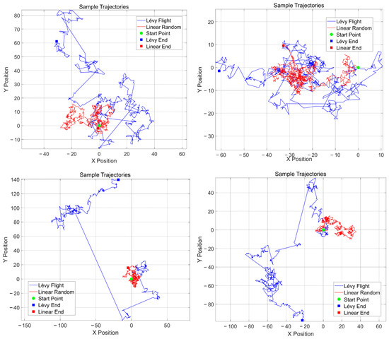
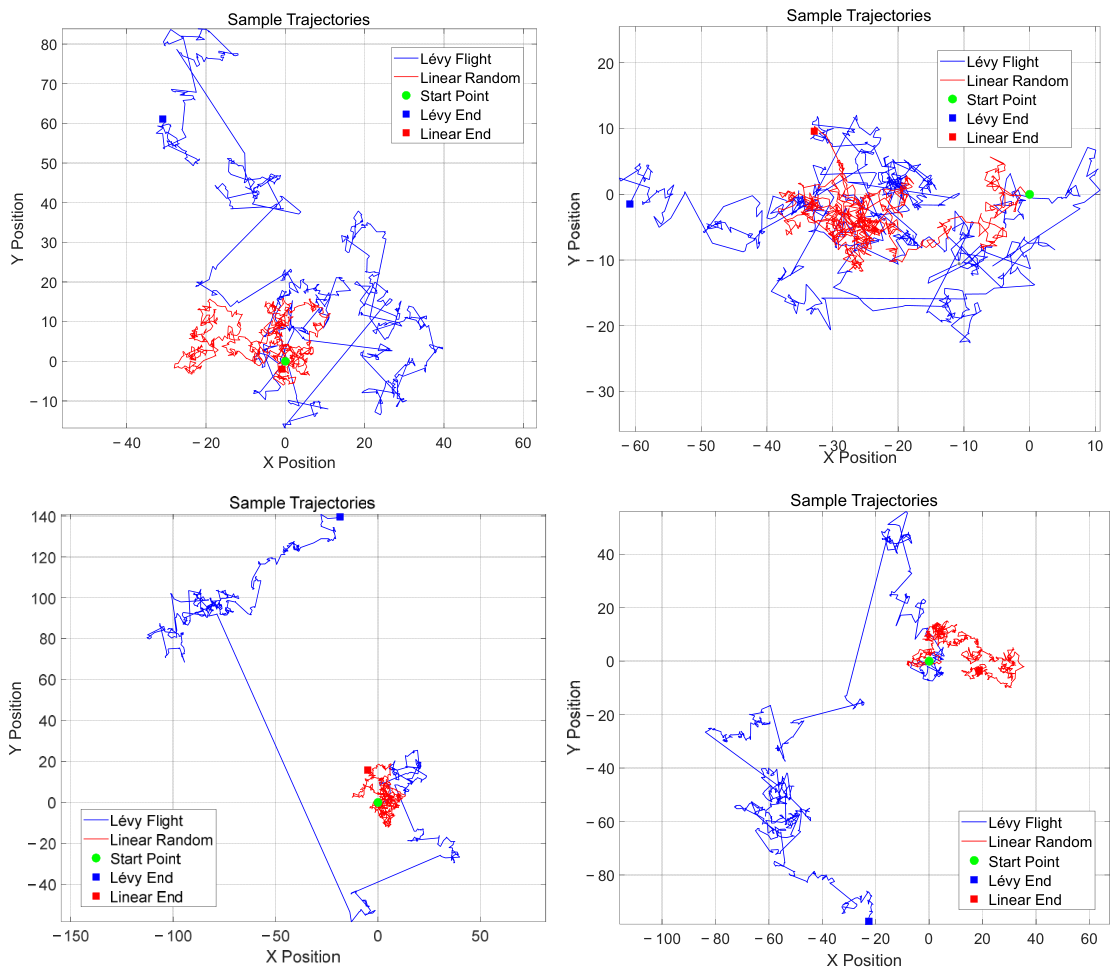
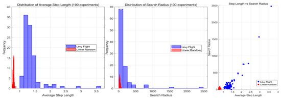
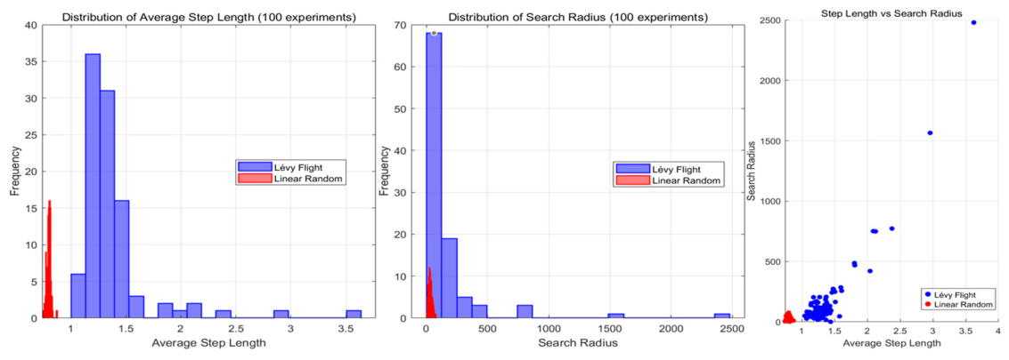
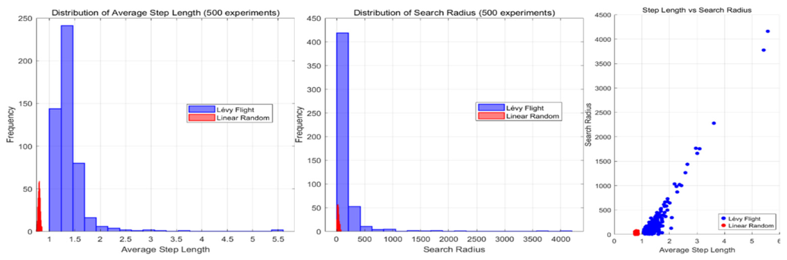
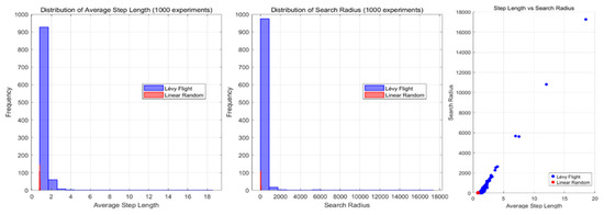
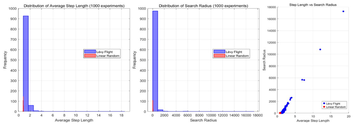
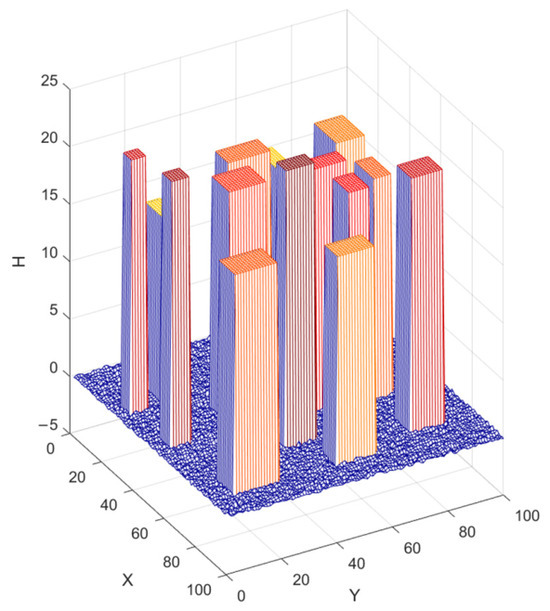
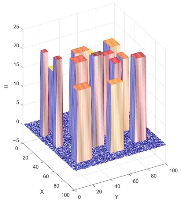
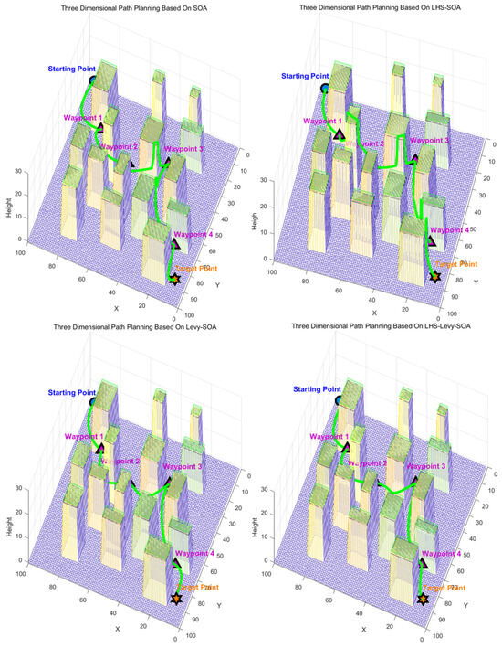
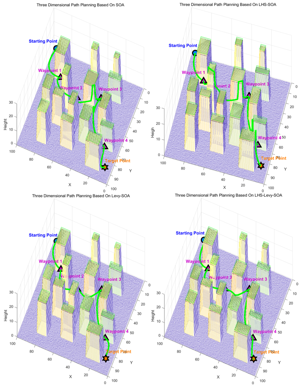
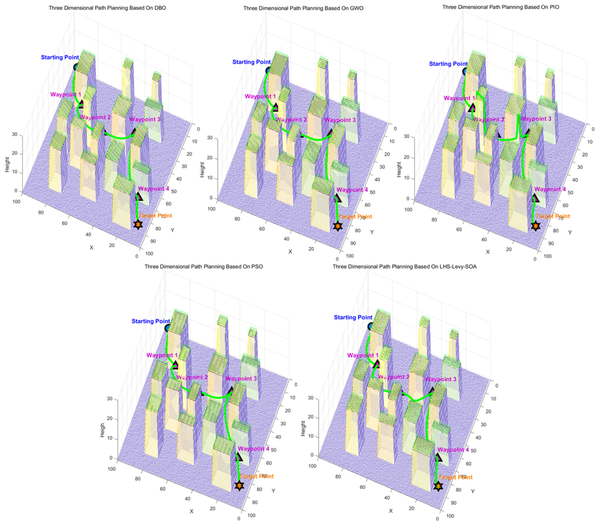
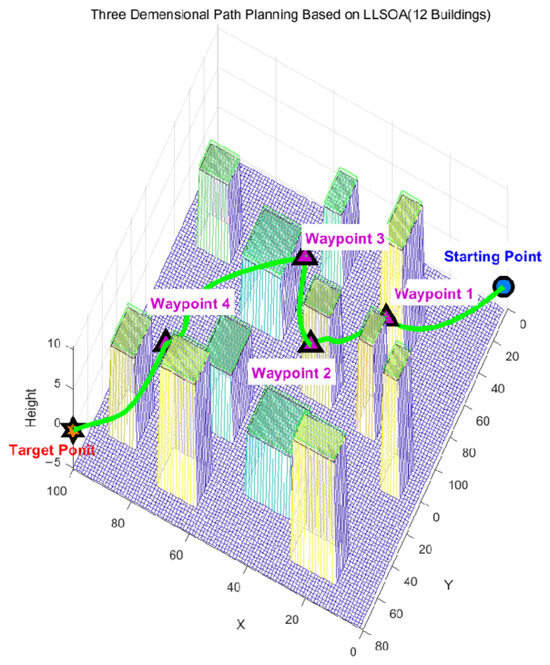
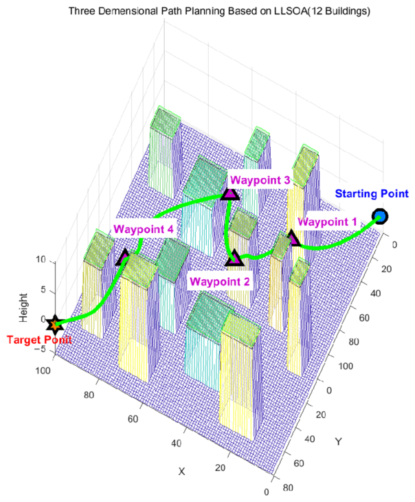
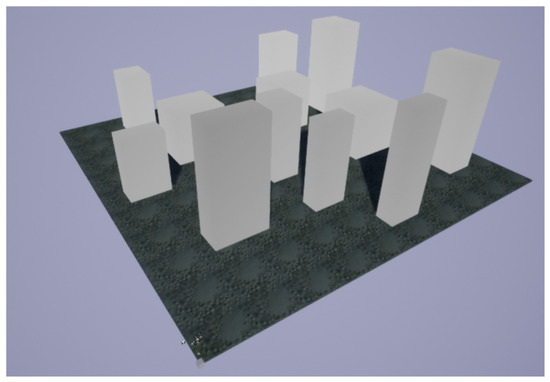
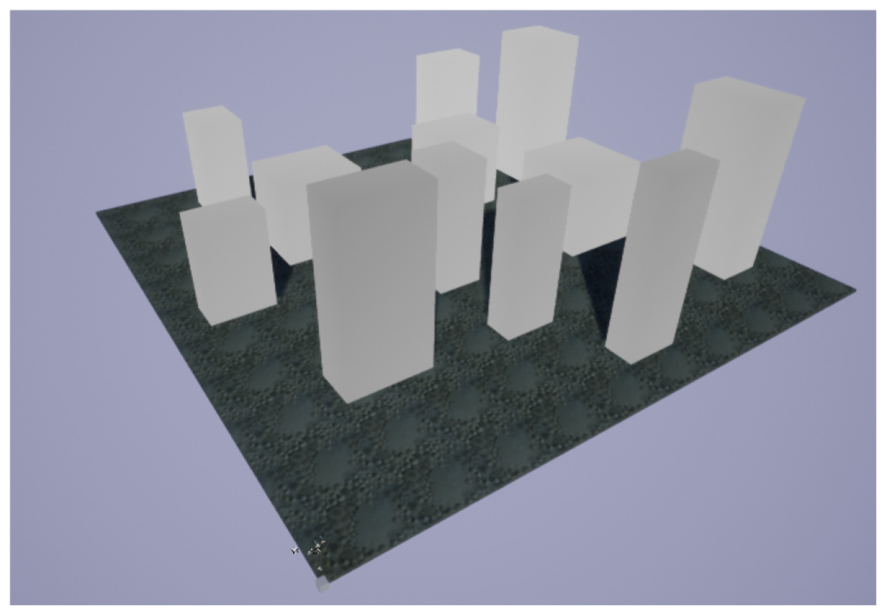
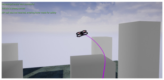
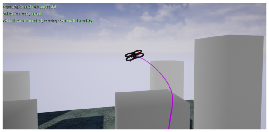

Disclaimer/Publisher’s Note: The statements, opinions and data contained in all publications are solely those of the individual author(s) and contributor(s) and not of MDPI and/or the editor(s). MDPI and/or the editor(s) disclaim responsibility for any injury to people or property resulting from any ideas, methods, instructions or products referred to in the content. |
© 2026 by the authors. Licensee MDPI, Basel, Switzerland. This article is an open access article distributed under the terms and conditions of the Creative Commons Attribution (CC BY) license.