Downwash–Spray Interactions in Agricultural Hexacopters: CFD Evaluation of Nozzle Configurations and Development of a Modular UAV Spray System

Highlights

What are the main findings?

• The placement of nozzles relative to rotor downwash significantly affects spray deposition uniformity, coverage, and drift behavior in UAV systems, with under-rotor configurations showing improved deposition uniformity and application efficiency compared to boom configurations, as confirmed by CFD results.
• The under-rotor two-nozzle configuration maximizes deposition area, application rate, and uniformity in the designed modular sprayer UAV with respective values of 9.375 m², 0.03387 mL/m², and 45.3%.

What are the implications of the main findings?

• CFD-informed design provides a reliable and efficient framework for optimizing UAV spraying systems before physical implementation.
• The results support the development of more efficient, adaptable UAV-based spraying strategies for precision agriculture, with potential benefits in reducing chemical waste and improving application effectiveness.

Abstract

Unmanned Aerial Vehicles (UAVs) are seeing increased use in agricultural settings due to their potential to be integrated with systems for applying pesticides. They can target specific areas while offering the potential to reduce chemical waste and improve application efficiency. However, this means that spray deposition efficiency is strongly influenced by rotor-induced downwash, which affects droplet transport, drift, and uniformity. This study presents a combined computational and experimental investigation of downwash–spray interactions in a hexacopter platform. CFD is used to predict the performance of various sprayer configurations that differ in the number, spacing, and positioning of nozzles. Rotor-induced airflow is modeled using an actuator disk approach in ANSYS Fluent 2025, and spray behavior is predicted using the Discrete Phase Model. Pure water was used as the working fluid for both the CFD simulations and experimental validation to ensure consistency between numerical and physical testing conditions. Numerical results indicate that a two-nozzle under-rotor setup maximizes performance characteristics such as deposition area, density, and uniformity for the designed agricultural UAV, providing a theoretically effective deposition area of 9.375 m², an effective application rate of 0.03387 mL/m², and a coefficient of variation of 45.3%. Compared to the best-performing boom configuration, this represents an approximately 13.5% improvement in spray uniformity. These results are validated through experimental testing using a modular UAV sprayer system and deposition measurements obtained from water-sensitive paper in controlled indoor conditions, achieving a droplet size of 502 µm, swath width of 1.8 m, 0.8% area coverage, and a coefficient of variation of 36.5%. While differences were observed between predicted and measured droplet size distributions, the CFD and experimental results demonstrated similar trends in spray coverage and deposition uniformity. Future work will refine simulations to better match experimental conditions and investigate canopy interaction, crosswind effects, and field-scale performance.

1. Introduction

UAVs have experienced significant growth in agricultural use, primarily due to their versatility. By equipping them with specialized systems, they can be used for applications such as monitoring crop health, predicting yield, and spreading seeds or pesticides. The integration of a pesticide sprayer system into a UAV is the primary focus of this study. When integrating a sprayer system into a UAV, the interactions between the spray and the rotor dynamics from the UAV must be properly considered, as they can affect each other in several ways [1]. The downwash from the rotors can disturb the canopies of the crops, which can allow for better penetration of the sprayed fluid, increasing effectiveness in some cases. This effect has been shown in prior studies to influence droplet deposition patterns and drift behavior, making it a critical consideration. This downwash also has the potential to direct the fluid droplets towards the intended crops, reducing waste and preventing contamination of nearby crops or water sources. The sprayer system can affect the performance of the UAV as well. The added weight of the system reduces the endurance of the UAV, either requiring a larger battery, which adds more weight, or more breaks to recharge to compensate [2]. Additionally, the presence of fluid in the sprayer system can negatively affect the maneuverability of the UAV, as the fluid can shift during flight [3]. These interactions between the flight and sprayer systems of an agricultural sprayer UAV must all be properly considered to ensure the efficiency of both systems is maximized. Therefore, understanding the coupled interaction between rotor dynamics and spray behavior is essential for optimizing UAV-based spraying systems.

Research findings from studies [4,5,6] have explored the potential advantages of UAV-based spraying systems in comparison to traditional application techniques, highlighting the need for further investigation into their practical use. While it is important to note that specific results are influenced by UAV performance parameters, each of these studies indicated a possible benefit from their implementation. These benefits include enhanced working efficiency in area coverage over time, more uniform deposition rates, and decreased water consumption. From an application technology perspective, improper interaction between rotor-induced airflow and sprayed droplets can contribute to several agronomic challenges, including off-target drift, insufficient canopy penetration, and non-uniform pesticide distribution. Excessive drift can reduce pesticide efficacy while increasing environmental contamination risks and economic losses due to inefficient chemical use. Conversely, inadequate droplet transport into the crop canopy may lead to poor pest and disease control. These competing effects make rotor–spray interactions a critical consideration when designing UAV spray systems and highlight the need to identify nozzle configurations that balance deposition uniformity, coverage, and drift mitigation.

1.1. Literature Context

The topic of this research was identified through a literature review, which demonstrated the current state and potential of the technology and procedures that could be implemented in this research. Articles such as [7,8,9] demonstrated that there were existing UAVs with the ability to complete agricultural tasks which traditionally rely on manual labor. The next articles which were examined, such as [10,11,12], were more focused specifically on the implementation of sprayer systems into agricultural UAVs. Though the types of sprayers and setups used in these articles do not all match what was used in this research, it served the purpose of highlighting the limitations of the technology and where this research could be focused. Other applications for UAVs in agriculture and their economic impact were also investigated during this stage of the literature review through articles like [13,14,15]. Though the focus of this research was on the development of spraying operations, the ability of UAVs to be used in other applications demonstrated their versatility and potential importance to agricultural operations. This is what led to versatility and modularity being a priority during this research, as it allows the final product to be potentially more cost-efficient while meeting the standards of the task.

The next stage of the literature review involved establishing the common practices which would be applied for observing system interaction and during numerical and experimental research. Some studies detailed approaches that are simple while being accurate enough for implementation in this research. The primary example of this is the actuator disk approach described in [16,17], which is a method for generating rotor dynamics in a simulation through a momentum source. This method is widely used due to its reduced computational cost compared to full rotor blade modeling, while still capturing overall flow behavior. Other studies like [18,19,20] obtain data regarding parameter values that are likely to maximize sprayer performance during testing. Such parameters include boundary conditions, domain dimensions, sprayer characteristics, and operating conditions such as altitude. These parameters strongly influence droplet transport and deposition, particularly in low-altitude UAV applications. The data regarding these parameters is especially beneficial to this study as it allows the focus of the data to remain on the effects specific sprayer characteristics have on the overall performance of the system. The sprayer characteristics being monitored include the number of nozzles as well as their spacing and positioning with respect to the rotors, with studies like [21,22,23] helping to identify these characteristics. Most reviewed studies highlight similar characteristics important for evaluating sprayer performance, namely coverage and uniformity. Coverage indicates how much fluid is being applied to the crops and is expressed through density and area measurements, while uniformity indicates how evenly the fluid is spread throughout that area, with a more even spread being more effective. These methodologies then provided the basis for how the numerical and experimental data in this study were evaluated. For this purpose, CFD is an important tool, as it allows these measurements to be taken under various conditions relatively quickly and easily, though verification of the results is necessary.

Additional articles, such as [3], also identified where there are limitations in current studies and the ability to implement UAVs in agriculture on a larger scale. These limitations primarily include the necessity for adequate consideration of rotor–sprayer interactions, limitations in UAV endurance, and the effects the presence of an integrated system has on the UAV and vice versa. However, many existing studies rely either on purely numerical simulations or on simplified experimental setups that do not fully capture the behavior of an operational UAV system. Acknowledging these limitations enables reflection on the approaches of this research and allows changes to be made that will further focus the research objectives on those that will address these limitations. It must also be stated that a large portion of the research presented in this study originates from work conducted for a master’s thesis at the University of Oklahoma [24], and a portion of the results are published in a conference paper for the IEEE Aerospace Conference 2026 [25].

1.2. Research Gap

As previously established, several studies investigate the influence of sprayer systems integrated into UAVs (Unmanned Aerial Vehicles). However, many of these studies either rely solely on numerical evaluations or use experimental setups that only replicate a UAV without directly observing how the sprayer system influences the UAV’s performance. One such study, referenced as [26], examines flow fields through simulation to predict their impact on pesticide application. The primary difference between their research and the present study lies in their experimental methods; they use a stationary rotor platform instead of a functional UAV. This characteristic is present in other studies as well, such as [27]. Consequently, their designed systems are likely aligned more with their simulated setup than with practical application. In contrast, this study aims to validate the functionality of the designed system through experimentation with a functional UAV. While the results may be somewhat less reflective of the simulations, they properly account for the size, weight, and cost limitations associated with implementing the sprayer system, making the findings more applicable to real-world operations.

Recent studies, such as [1,28,29], have experimentally tested sprayer system performance using functional UAVs in agricultural settings. However, this study seeks to improve upon the experimental approaches of these articles by focusing on design characteristics. Most articles reviewed that involve practical experimentation concentrate on the overall outcomes of the testing—essentially determining whether the UAV-mounted sprayer system can perform as desired compared to traditional methods. A more nuanced analysis of how the design of the UAV and the sprayer system affects performance characteristics could yield valuable insights into the benefits and tradeoffs of implementing this technology.

Finally, this study aims to fill the research gaps identified in other works by prioritizing design parameters over performance parameters. While many articles that experimentally investigate UAV spraying operations, such as [30], examine operational factors like flight speed, wind speed, or altitude and their effects on sprayer performance, there appears to be a lack of research on the influence of design aspects, such as nozzle spacing or quantity. Although [30] does not focus on pesticide sprayer systems for UAVs, their approach to testing the designed delivery device has inspired a greater emphasis on design characteristics in this study. Beyond methodological limitations, a practical agricultural challenge remains regarding the selection of nozzle placement strategies for UAV spray systems. Traditional boom-mounted configurations are commonly used because they increase potential spray coverage; however, wider coverage can also increase droplet dispersion and reduce deposition uniformity. Conversely, positioning nozzles closer to the rotor downwash may improve deposition concentration and reduce drift but may limit overall coverage area. The extent to which these competing effects influence spray performance remains insufficiently understood, particularly for small agricultural UAV platforms. Addressing this knowledge gap is important for improving application efficiency while minimizing drift-related losses and environmental impacts.

1.3. Hypothesis

This study hypothesizes that nozzle placement beneath the rotor downwash core will improve spray deposition uniformity and application efficiency compared with conventional boom-mounted configurations. The hypothesis is based on the premise that droplets introduced directly into the high-velocity downwash core experience greater downward momentum and reduced exposure to lateral transport mechanisms associated with rotor-tip vortices. As a result, under-rotor configurations are expected to produce more concentrated deposition patterns and reduced drift potential under controlled operating conditions.

1.4. Objectives and Contributions

The work conducted in this study aims to use both simulation and experimentation to identify how characteristics of a sprayer system, such as the number of nozzles, their spacing, and positioning with respect to the rotors, can affect the performance of the system and the UAV into which it is integrated. Therefore, the primary research objectives are the use of CFD to collect numerical data regarding the effects of the mentioned characteristics on the performance of the potential sprayer system design and the UAV.

The first objective focuses on the purpose of the simulations run for this research. The simulations are meant to test nozzle placement in different sprayer system configurations. These configurations include both boom-based and under-rotor nozzle setups, selected to represent common design approaches in UAV spraying systems. The boom configuration is tested in four setups with varying characteristics, while the under-rotor configuration has two, allowing for conclusions to be drawn regarding various parameters.

The second objective is to use these preliminary conclusions to make decisions regarding the design of the experimental UAV and the integrated modular sprayer system.

The third objective is to validate conclusions drawn from the numerical results. The data obtained during experimentation is ultimately meant to prove consistency between numerical and experimental data regarding the observed deposition characteristics under controlled conditions. Validation is performed through comparison of characteristics such as uniformity and coverage between simulation and experimental measurements.

To the authors’ knowledge, this work represents one of the few studies that combines CFD-based optimization of UAV spray-system geometry with full-scale experimental validation on a functional agricultural UAV platform. Furthermore, the study directly evaluates the influence of nozzle placement relative to rotor downwash, providing insight into the tradeoff between deposition uniformity and coverage area that has received limited attention in previous UAV spraying research.

This study will address the research gap through the gathering of both numerical and experimental data, with the numerical CFD analysis serving the purpose of narrowing the focus of the experimental trials and informing the design of a sprayer system to be implemented into an assembled functional UAV. This combined approach represents a key contribution of this work by linking simulation-based optimization directly with full-system experimental validation. The experimental tests are then meant to demonstrate the ability of the final UAV to perform as expected and validate the numerical data by reproducing its results.

Additionally, the UAV designed over the course of this research is meant to provide benefits over most commercially available models. The UAV itself is small and cheap while still having the capacity to be integrated with the sprayer system, making it beneficial for use in smaller-scale agricultural operations. The sprayer system is integrated with the primary benefits of being modular and reconfigurable, meaning it can be easily detached from the UAV, allowing for the UAV to be used for other applications in addition to spraying. The reconfigurability of the sprayer system then provides the benefit of allowing the performance characteristics of the system to be changed relatively easily, so that the whole system itself can be applied to another agricultural UAV with a different frame.

2. Materials and Methods

2.1. UAV Platform and Operating Conditions

The first step of developing a model in CFD to represent an agricultural UAV is creating a platform representative of the UAV intended to be used during experimental testing. The aspects of this designed UAV that affect the model in CFD are primarily the frame and propellers. These geometric features directly influence rotor-induced airflow and therefore must be represented accurately for reliable simulation results. However, the initial expected capabilities of the flight system and its components must also be determined, as they define the operating conditions used in the simulations, particularly the thrust required to maintain hover.

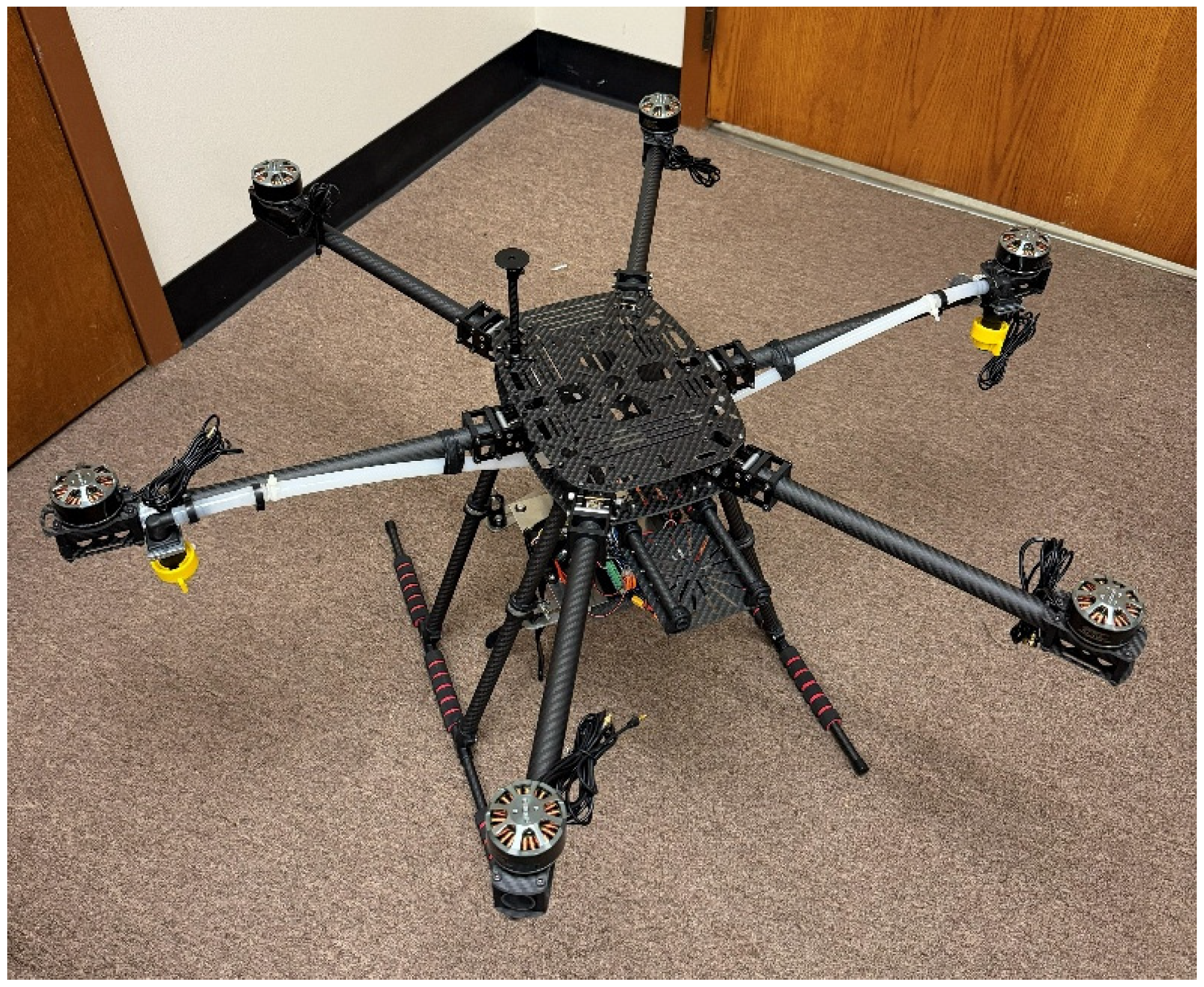
The primary criteria for components considered for the initial UAV design are based on availability and price. The selected frame is the JMT ZD850 hexacopter (JMT Direct Store, Hongkong) frame shown in Figure 1. The frame has a length of 0.85 m and a payload capacity of 7 kg, which informs the takeoff weight of the final UAV and the selection of the remaining components. These specifications are also used to estimate total thrust requirements for the actuator disk model.

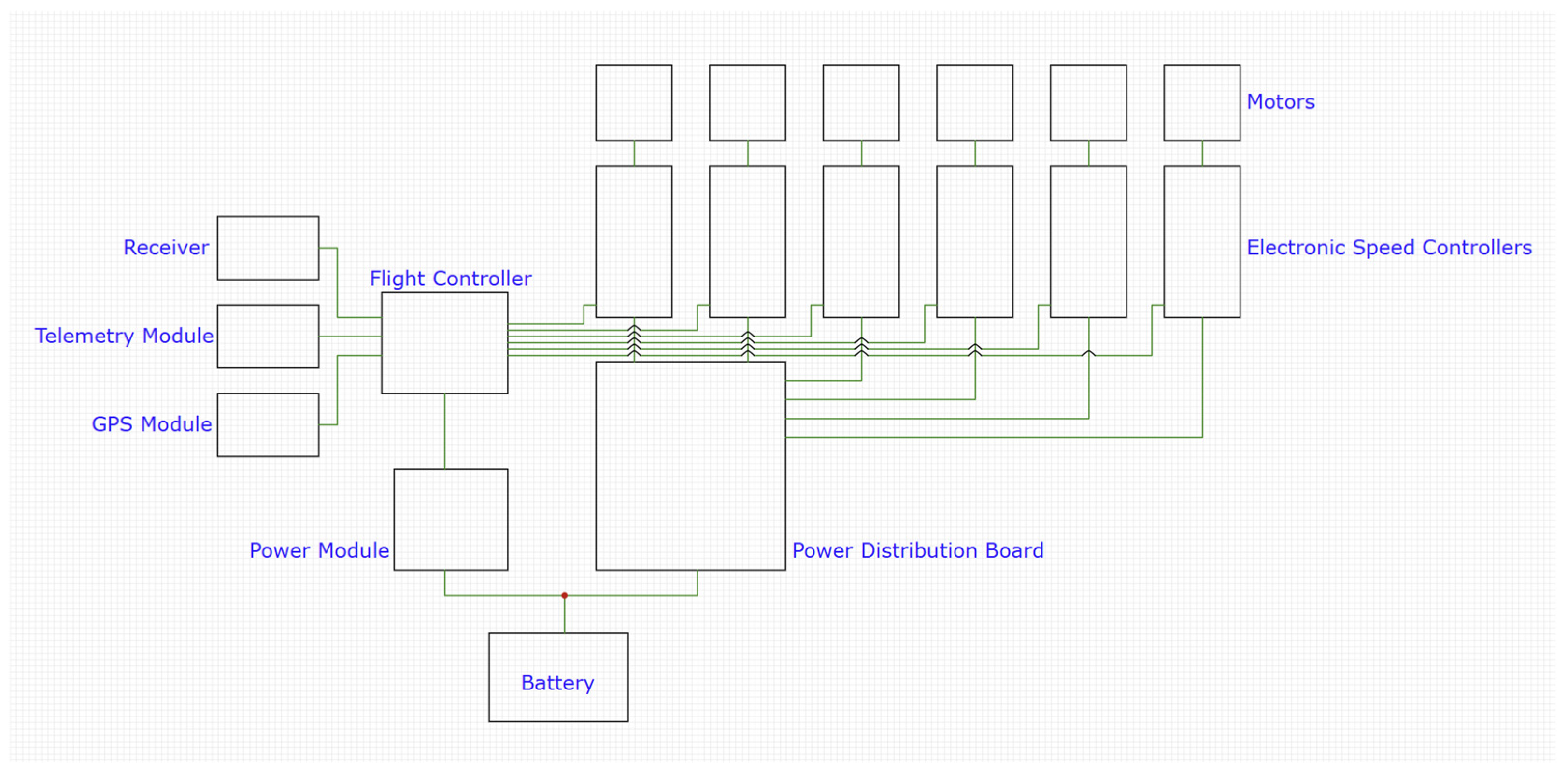
The components were also selected with specific performance goals in mind, specifically a flight time of about 10 min and a thrust-to-weight ratio of 2. A thrust-to-weight ratio of 2 was selected to ensure stable hover and maneuverability under load. However, not all of these performance goals were met exactly, primarily due to changes made during the assembly of the UAV with goals of using more accessible parts or allowing for more flexibility with the design of the sprayer system. The wiring diagram of the UAV flight configuration is shown in Figure 2. The specifications of the UAV platform are as shown in

Table 1. UAV Specifications.

Feature	Description
Total Takeoff Weight	6.2 kg
Sprayer System Weight	2.5 kg
Thrust-to-Weight Ratio	1.8
Flight Time	~8 min
Flight Controller	Pixhawk 6C Mini
Motor	400 KV Brushless Motor (Gartt-rc, Shenzhen, China)
Battery	6S 6000 mAh LiPo Battery (Ovonic Direct, Hongkong)
Propeller	1447 Carbon Fiber Propeller (QwinOut, Hongkong)
Nozzle	TeeJet XR110015VS Nozzle (Simpson Farm Enterprises, Beloit, KS, USA)
Pump	R385 Diaphragm Pump 1.5–2.0 L/min (12 V) (FangshenStore, China)

. The flight controller is the Pixhawk 6C Mini-Model A (Holybro, Hong Kong, China), which comes with the M9N GPS Module and PM02 V3 Power Module.

2.2. CFD Domain, Mesh, and Boundary Conditions

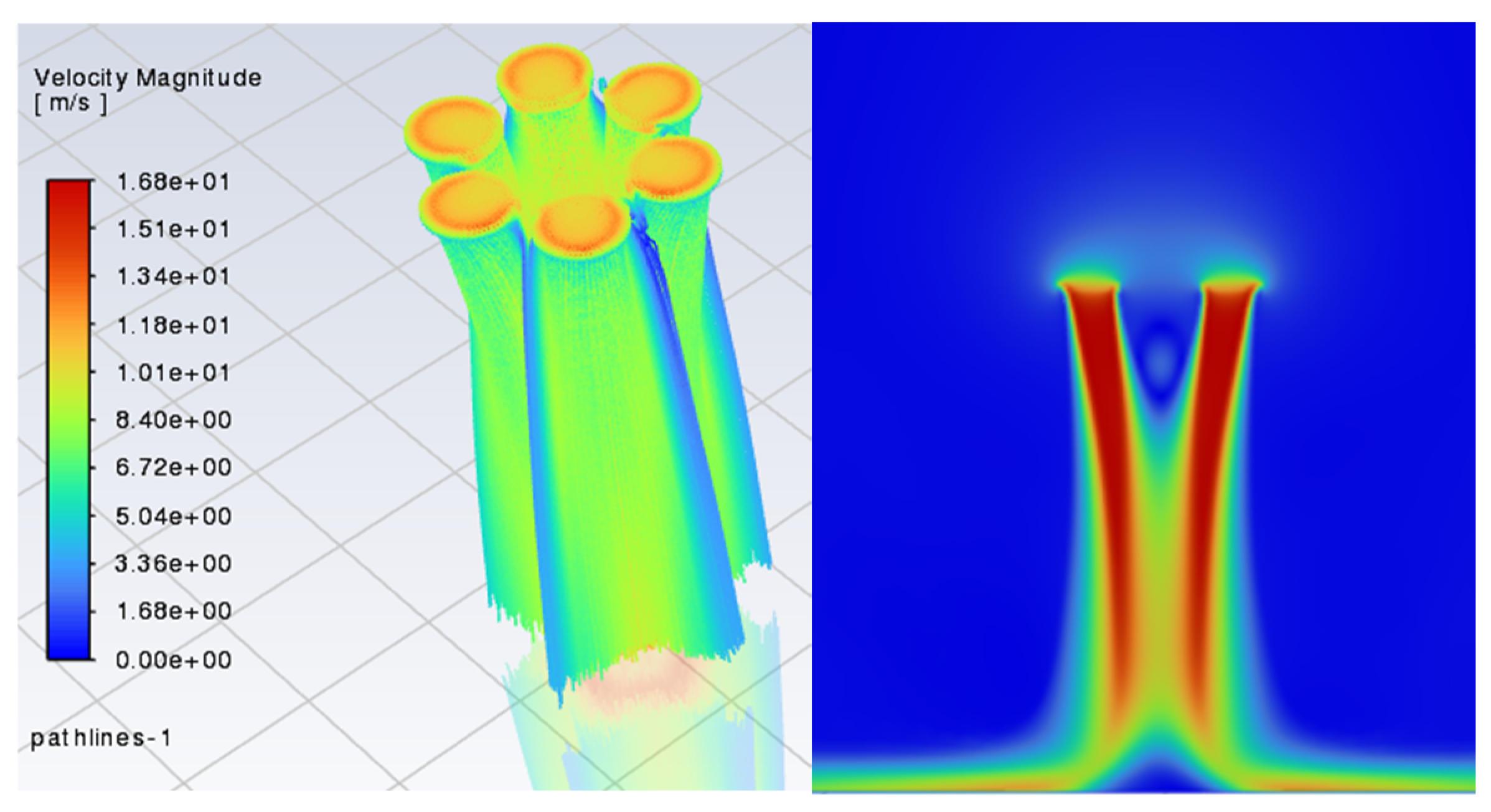
Numerical simulations in this study are conducted with ANSYS Fluent, and the UAV geometry is created with ANSYS Design Modeler. The simulations are performed under steady-state conditions to approximate hover behavior. The geometry consists of a 10 × 10 × 5 m domain, actuator disks representing rotors, and a cylindrical region of influence. The domain size is selected to minimize boundary effects on rotor-induced flow [18]. The bottom face is treated as a no-slip wall representing the ground, while the remaining faces are pressure outlets. This setup allows airflow to exit freely, preventing artificial recirculation at domain boundaries. 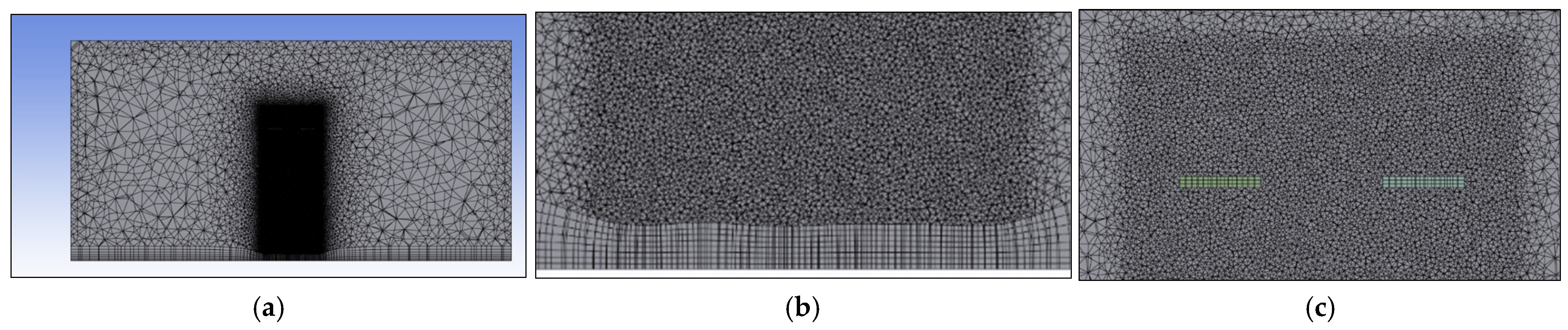The centers of the actuator disks are positioned 3 m above the ground plane and oriented to align with the size of the selected frame [19]. The base mesh used in the CFD analysis is shown in Figure 3 and comprises 6,496,806 elements and 1,156,459 nodes.

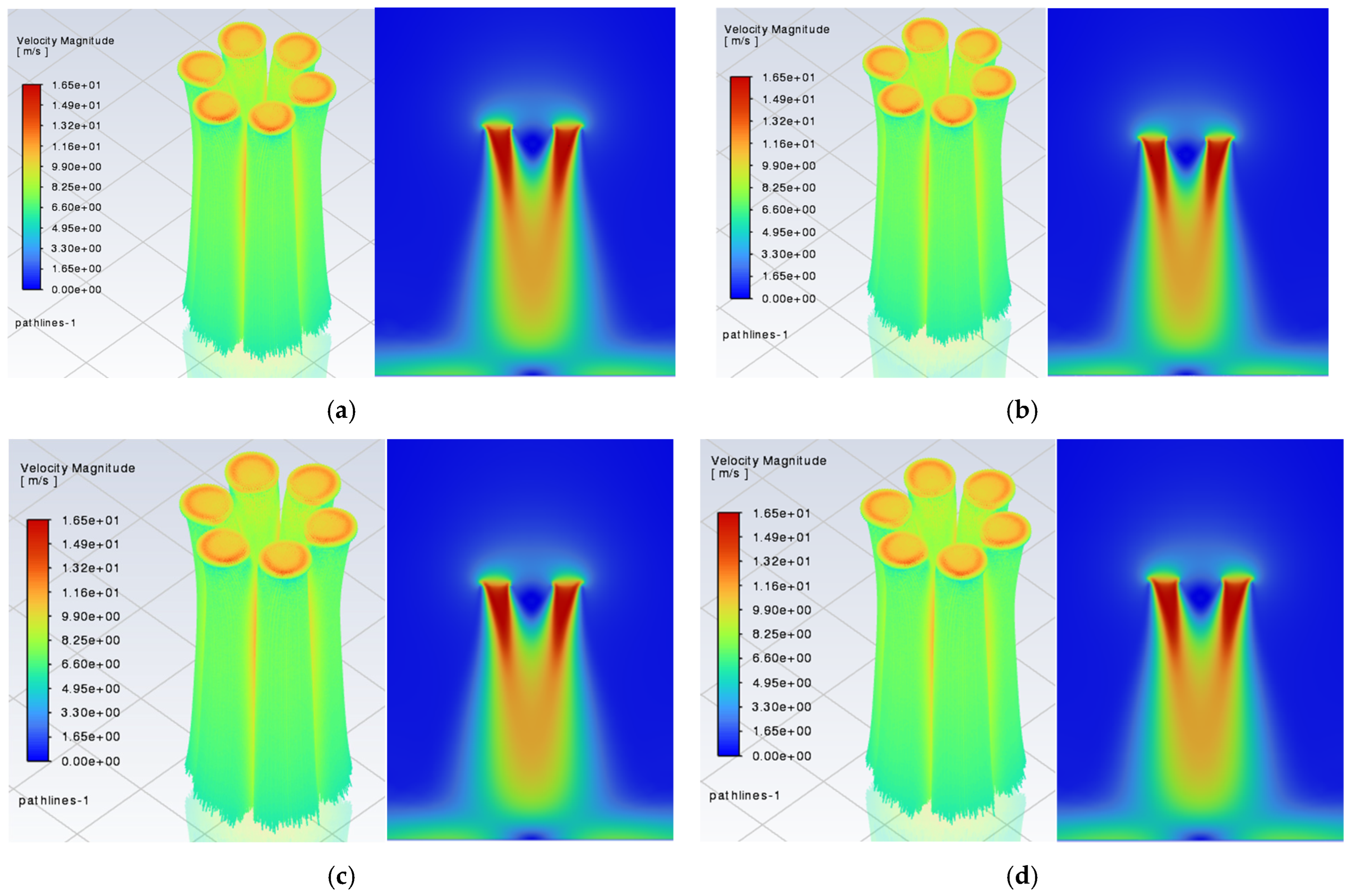
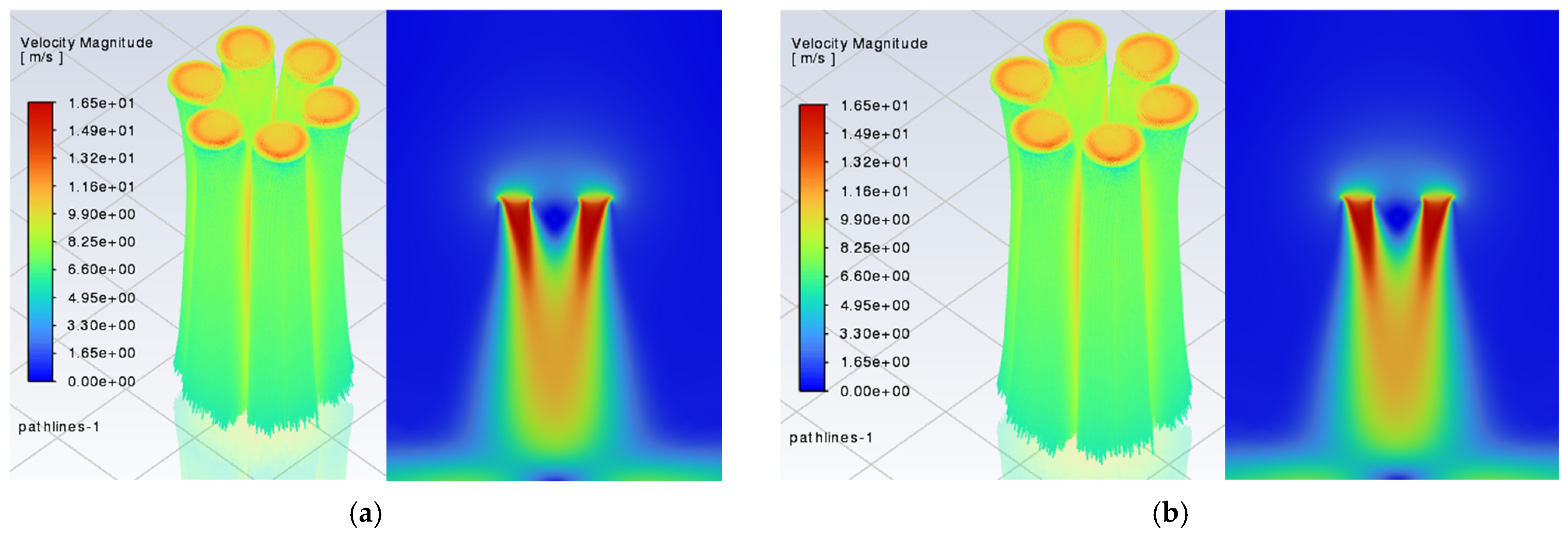
A mesh independence study is conducted to validate the results obtained with the base mesh. Mesh convergence is assessed using velocity magnitude and Y+ values. The criterion for independence is that values across meshes are within 5% of each other. This threshold is commonly used in CFD studies to ensure numerical accuracy without high computational cost. As shown in

Table 2. Mesh Independence Study Results.

Mesh	Global Element Size (m)	Y+ Value	Average Velocity Magnitude (m/s)
			Value	Error (%)
M0	0.2	26.2 to 177	0.2655
M1	0.3	46.3 to 684	0.2159	18.7
M2	0.15	4.01 to 108	0.4854	82.8
M3	0.1375	1.27 to 77.8	0.5381	10.8
M4	0.125	1.75 to 50.1	0.5705	6.02
M5	0.12	0 to 39.1	0.5775	1.23

, Y+ values decrease with mesh refinement while velocity magnitude increases [31]. These trends are accompanied by continuity residuals in the range of 10⁻⁵, indicating convergence between iterations. Additionally, convergence in the physical quantities of the simulation is a significant indicator of overall convergence. For this research, which aims to use CFD to inform UAV design and predict experimental outcomes, the physical quantities are considered sufficient to indicate convergence when accompanied by the given continuity residuals. Between M4 and M5 meshes, the average velocity magnitude changed by only 1.23%, satisfying the selected mesh-independence criterion and confirming that further refinement would provide limited benefit relative to the computational cost.

2.3. Rotor Modeling and Turbulence Model

The purpose of using an actuator disk approach in this research is to represent rotor-induced airflow while maintaining computational efficiency. Rather than explicitly resolving blade geometry, the method approximates rotor effects through a momentum source term, allowing the dominant characteristics of the downwash flow field to be captured at a significantly lower computational cost than blade-resolved simulations. Since the primary objective of this study is to compare the relative effects of different nozzle configurations on spray deposition rather than to investigate detailed rotor aerodynamics, the actuator disk approach provides an appropriate level of modeling fidelity. The momentum provided by each disk is determined to be 4280.33 N/m³ based on hover conditions, where total thrust equals UAV weight. The UAV modeled in this study has a total takeoff weight of 6.2 kg, corresponding to a gravitational force of approximately 60.8 N. Assuming equal load distribution across the six rotors, each rotor is required to generate approximately 10.1 N of thrust to maintain hover. These operating conditions were used to define the actuator disk source term and ensure that the simulated flow field represents equilibrium flight conditions.

The simulations use the SST k-omega turbulence model to capture wake behavior. This model is selected due to its improved performance in predicting adverse pressure gradients and separating flows compared to the k-epsilon model [16]. The SST k-omega turbulence model uses two transport equations. The first is for k, which is given by the equation

$${\displaystyle \frac{\partial }{\partial \mathrm{t}}}\left(\mathsf{\rho }\mathrm{k}\right)+{\displaystyle \frac{\partial }{\partial {\mathrm{x}}_{\mathrm{i}}}}\left(\mathsf{\rho }\mathrm{k}{\mathrm{u}}_{\mathrm{i}}\right)={\displaystyle \frac{\partial }{\partial {\mathrm{x}}_{\mathrm{i}}}}\left({\displaystyle \frac{\partial \mathrm{k}}{\partial {\mathrm{x}}_{\mathrm{i}}}}\left(\mathsf{\mu }+{\displaystyle \frac{{\mathsf{\mu }}_{\mathrm{t}}}{{\mathsf{\sigma }}_{\mathrm{k}}}}\right)\right)+{\mathsf{\mu }}_{\mathrm{t}}{\mathrm{S}}^2-{\mathsf{\beta }}^{*}\mathsf{\rho }\mathrm{k}\mathsf{\omega }$$

(1)

where $\rho$ is the fluid density, k is the turbulent kinetic energy, u is the velocity component, $\mu$ is the molecular viscosity, ${\mu }_t$ is the turbulent viscosity, and S is the strain rate magnitude. These variables are also present in the omega transport equation

$${\displaystyle \frac{\partial }{\partial \mathrm{t}}}\left(\mathsf{\rho }\mathsf{\omega }\right)+{\displaystyle \frac{\partial }{\partial {\mathrm{x}}_{\mathrm{i}}}}\left(\mathsf{\rho }{\mathrm{u}}_{\mathrm{i}}\mathsf{\omega }\right)=\mathsf{\alpha }{\mathsf{\mu }}_{\mathrm{t}}{\mathrm{S}}^2{\displaystyle \frac{\mathsf{\omega }}{\mathrm{k}}}-\mathsf{\beta }\mathsf{\rho }{\mathsf{\omega }}^2+{\displaystyle \frac{\partial }{\partial {\mathrm{x}}_{\mathrm{i}}}}\left({\displaystyle \frac{\partial \mathsf{\omega }}{\partial {\mathrm{x}}_{\mathrm{i}}}}\left(\mathsf{\mu }+{\mathsf{\sigma }}_{\mathsf{\omega }}{\mathsf{\mu }}_{\mathrm{t}}\right)\right)+2\left(1-{\mathrm{F}}_1\right)\mathsf{\rho }{\mathsf{\sigma }}_{\mathsf{\omega }2}{\displaystyle \frac{1}{\mathsf{\omega }}}{\displaystyle \frac{\partial \mathrm{k}}{\partial {\mathrm{x}}_{\mathrm{i}}}}{\displaystyle \frac{\partial \mathsf{\omega }}{\partial {\mathrm{x}}_{\mathrm{i}}}}$$

(2)

and the turbulent (eddy) viscosity equation, which is used in SST modeling,

$${\mathsf{\mu }}_{\mathrm{t}}={\displaystyle \frac{\mathsf{\rho }{\mathrm{a}}_1\mathrm{k}}{\max \left({\mathrm{a}}_1\mathsf{\omega },\mathrm{S}{\mathrm{F}}_2\right)}}$$

(3)

where $F_1$ and $F_2$ are Menter blending functions and α, β, β*, σ_k, σ_ω, σ_ω2, and a₁ are all constants.

2.4. Spray Modeling (Discrete Phase Model)

The spray injection is simulated using the Discrete Phase Model (DPM), which tracks droplet trajectories. A Lagrangian particle tracking approach is used to account for droplet–air interaction. This tracks particle position until it either encounters the ground plane or one of the pressure outlets, in which case it is counted as trapped or escaped. Droplet drag is evaluated using the spherical drag law and turbulent dispersion using the discrete random walk method. The discrete random walk method determines effective particle velocity by adding instantaneous fluctuations to the mean velocity. The core equations for the rest of the model are given by

$${\displaystyle \frac{\mathrm{\pi }}{6}}{\mathsf{\rho }}_{\mathrm{p}}{\mathrm{d}}^3{\displaystyle \frac{\mathrm{d}}{\mathrm{d}\mathrm{t}}}\left({\mathbf{u}}_{\mathrm{p}}\right)={\mathbf{F}}_{\mathrm{D}}+{\displaystyle \frac{\mathrm{\pi }}{6}}{\mathsf{\rho }}_{\mathrm{p}}{\mathrm{d}}^3\mathbf{g}$$

(4)

$${\mathbf{F}}_{\mathrm{D}}={\displaystyle \frac{1}{2}}{\mathrm{C}}_{\mathrm{D}}\mathsf{\rho }{\displaystyle \frac{\mathrm{\pi }}{4}}{\mathrm{d}}^2\left|\mathbf{u}-{\mathbf{u}}_{\mathrm{p}}\right|\left(\mathbf{u}-{\mathbf{u}}_{\mathrm{p}}\right)$$

(5)

and

$${\mathrm{C}}_{\mathrm{D}}={\displaystyle \frac{24}{\mathrm{R}\mathrm{e}}}\left(1+0.15{\mathrm{R}\mathrm{e}}^{0.687}\right)$$

(6)

where ρ is the fluid density, ρ_p is the density of the particle, d is the particle diameter, u is the local fluid velocity, u_p is the droplet velocity, F_D is the drag force, g is the acceleration due to gravity, and CD is the drag coefficient. In the case of Equation (6), it only applies to Reynolds numbers less than 1000. If the value is greater than or equal to 1000, then the drag coefficient is assumed to be 0.44 [32].

Droplet sizes follow a Rosin–Rammler distribution with a mean diameter of 300 µm as defined by the following equations

$$\mathrm{F}\left(\mathrm{d}\right)=1-{\mathrm{e}}^{-{({\displaystyle \frac{\mathrm{d}}{\mathrm{\lambda }}})}^{\mathrm{n}}}$$

(7)

$$\mathrm{f}\left(\mathrm{d}\right)={\displaystyle \frac{\mathrm{n}}{\mathrm{\lambda }}}{({\displaystyle \frac{\mathrm{d}}{\mathrm{\lambda }}})}^{\mathrm{n}-1}{\mathrm{e}}^{-{({\displaystyle \frac{\mathrm{d}}{\mathrm{\lambda }}})}^{\mathrm{n}}}$$

(8)

$$\mathrm{\lambda }={\displaystyle \frac{\overline{\mathrm{d}}}{\mathrm{\Gamma }\left(1+\frac{1}{\mathrm{n}}\right)}}$$

(9)

where d is a given droplet diameter, $\overline{\mathrm{d}}$ is the mean droplet diameter, F(d) is the mass fraction function for that diameter, f(d) is the probability density function for that diameter, λ is the scale parameter, Γ is the gamma function, and n is the spread parameter, which is 2 in this study. A mean diameter of 300 µm was selected for the simulations based on the nozzle type that was expected to be available when developing the conceptual design of the sprayer system. This distribution represents typical agricultural spray characteristics based on commercial nozzle specifications. Droplet evaporation and secondary breakup are neglected, which is a reasonable assumption for short travel distances and large droplet sizes. Although evaporation and secondary breakup may influence droplet transport under field conditions, their effects are expected to be limited for the relatively large droplets and short travel distances considered in this study. Therefore, the simulations should primarily be interpreted as representations of deposition trends rather than exact droplet-size evolution.

2.5. Nozzle Configurations Evaluated

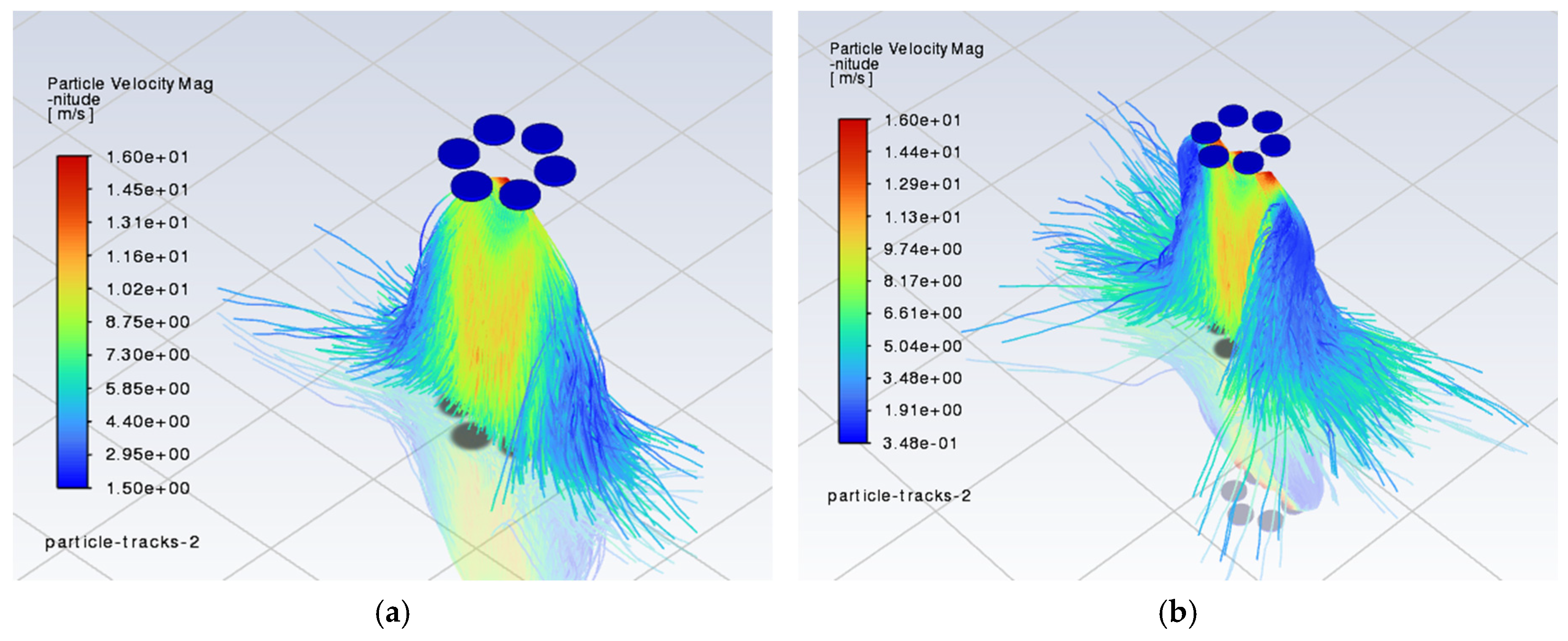
Four boom configurations and two under-rotor configurations shown in

Table 3. Nozzle Configurations.

Configuration	Setup	Number of Nozzles	Nozzle Spacing (m)
C1	Boom	1	N/A
C2	Boom	3	0.5
C3	Boom	2	1
C4	Boom	2	0.6
C5	Under-Rotor	2	0.6495
C6	Under-Rotor	2	0.75

are simulated for this research. These configurations were selected to represent commonly used UAV spraying layouts and to evaluate the influence of nozzle placement relative to rotor flow. The performance is evaluated based on deposition density, uniformity, and area. Deposition uniformity is quantified using the coefficient of variation (CV%). The goal of these comparisons is to determine which setup maximizes sprayer system performance to prepare for the implementation of a sprayer system in experimental trials.

The first boom configuration (C1) employs a single nozzle positioned below the center point between the actuator disks. The second boom configuration (C2) adds two other nozzles positioned 0.5 m on either side of the original nozzle so that their 110-degree arches intersect, and the resulting spray pattern forms a line. The third boom configuration (C3) removes the original center nozzle, and the fourth (C4) brings the two remaining nozzles closer together so that they are each positioned 0.3 m away from the center. The spacing in the different setups is determined based on [20], where 0.6 m is cited as the optimal nozzle spacing. The spacing in the second and third setups is slightly smaller to maintain simplicity and limit the size of the spar.

The under-rotor setup employs only two configurations due to the reduced potential for variability that comes from the symmetry of the different potential configurations. Both configurations use two nozzles placed directly underneath the rotors, translated 0.05 m closer to the center of the frame from the center of the rotor. The vertical location of the nozzles relative to the rotor plane was kept constant for both under-rotor configurations so that any differences in performance could be attributed primarily to nozzle placement rather than release height. The first configuration (C5) places the nozzles directly under the front two rotors. The second (C6) uses the nozzles under the center rotors instead.

2.6. Quantitative Deposition Analysis

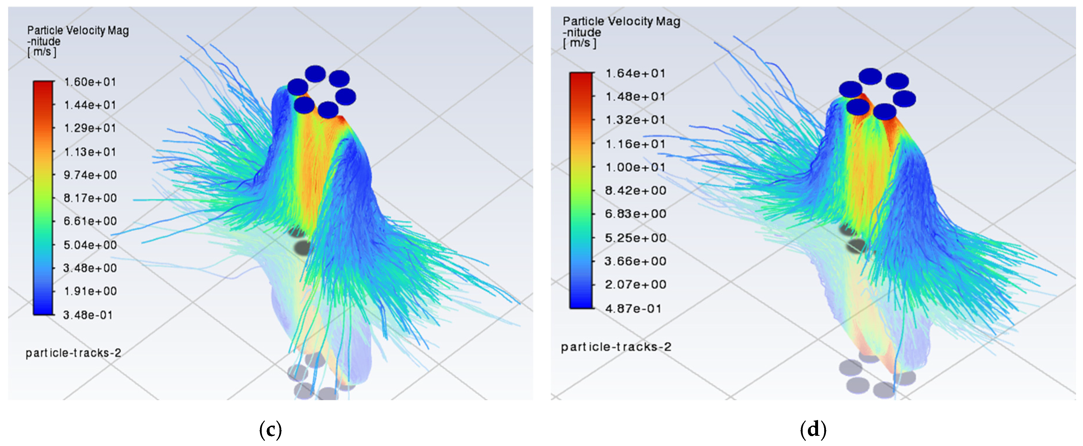
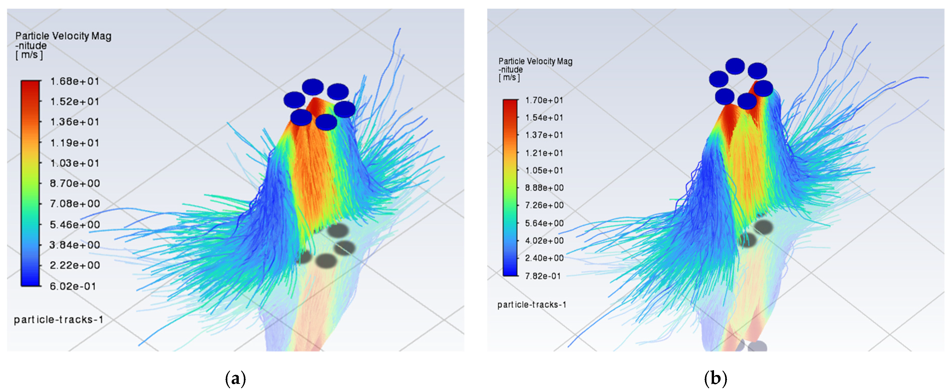
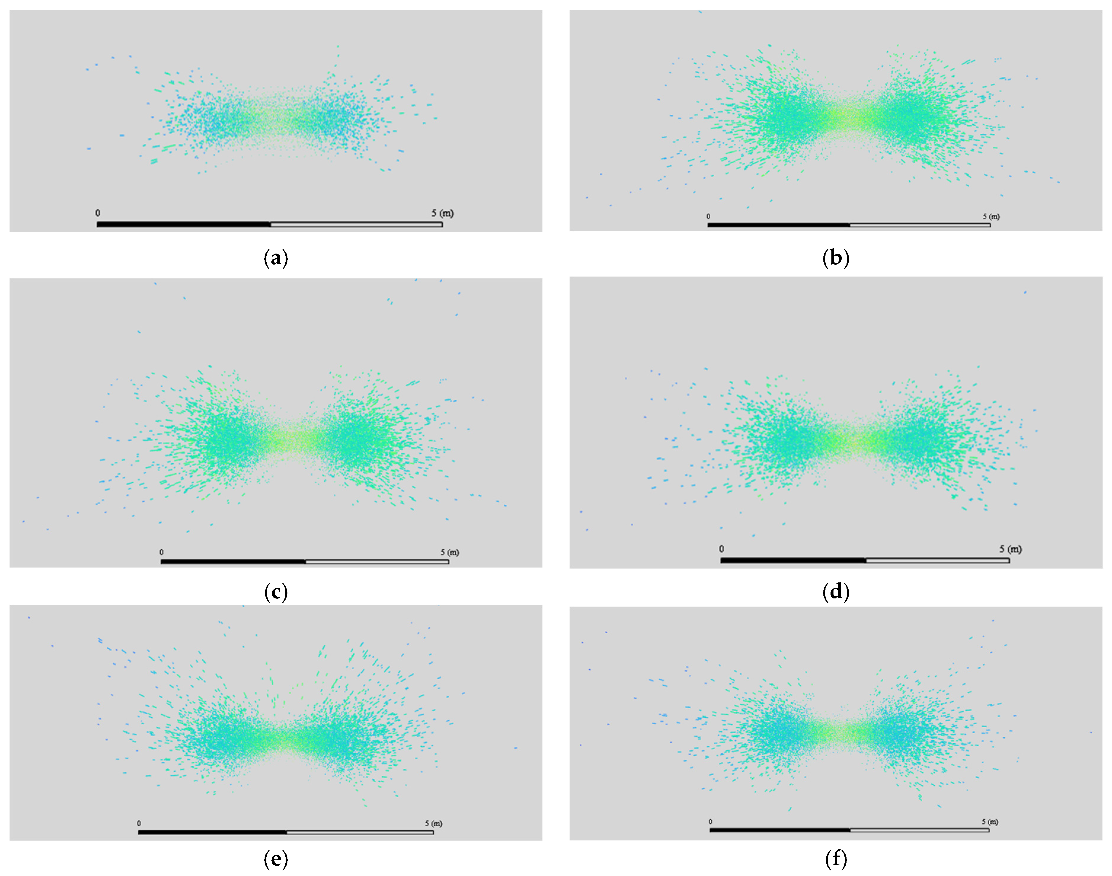
The simulations are evaluated using key metrics, including deposition rate, application rate, and uniformity. These metrics are derived from particle impact data recorded at the ground plane. The particle tracks demonstrate the impact of the downwash on the trajectory of the sprayed fluid, enabling conclusions regarding the influence of different parameters. Deposition areas of the configurations are measured both qualitatively and quantitatively using visualization of where the particle tracks intersected with the ground plane and particle position data.

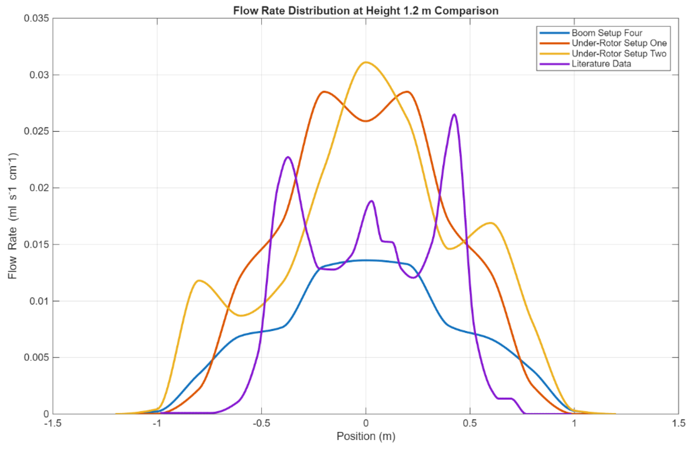
The first metric is the rate at which the sprayed fluid meets the ground plane, which is calculated using the equation

$$\mathrm{Q}={\displaystyle \frac{\mathrm{V}\mathrm{n}}{\mathrm{L}\mathrm{t}}}$$

(10)

where Q is the volumetric flow rate per unit length, V is the volume of each particle, n is the number of particles within a specified region of the deposition area, L is the maximum depth of the deposition area, and t is the total time over which particles are being deposited on the ground plane [17].

The application rate is used for comparing configurations within this study, given by the equation

$$\mathrm{q}={\displaystyle \frac{\mathrm{V}\mathrm{n}}{\mathrm{L}∆\mathrm{X}}}$$

(11)

where q is the volumetric application rate, and ΔX is the length of the small portion of the deposition area’s width in which fluid volume is being measured.

The coefficient of variation (CV%) is used as a measure of uniformity. Lower CV% values indicate more uniform spray distribution, and the CV% should ideally be between 15 and 30% [20]. The CV% is given by the equation

$$\mathrm{C}\mathrm{V}\%=100·{\displaystyle \frac{\mathrm{s}}{\overline{\mathrm{X}}}}$$

(12)

where s is the sample standard deviation of the volumes of fluid, and $\overline{\mathrm{X}}$ is the mean of those values.

2.7. Modular Spray System Design

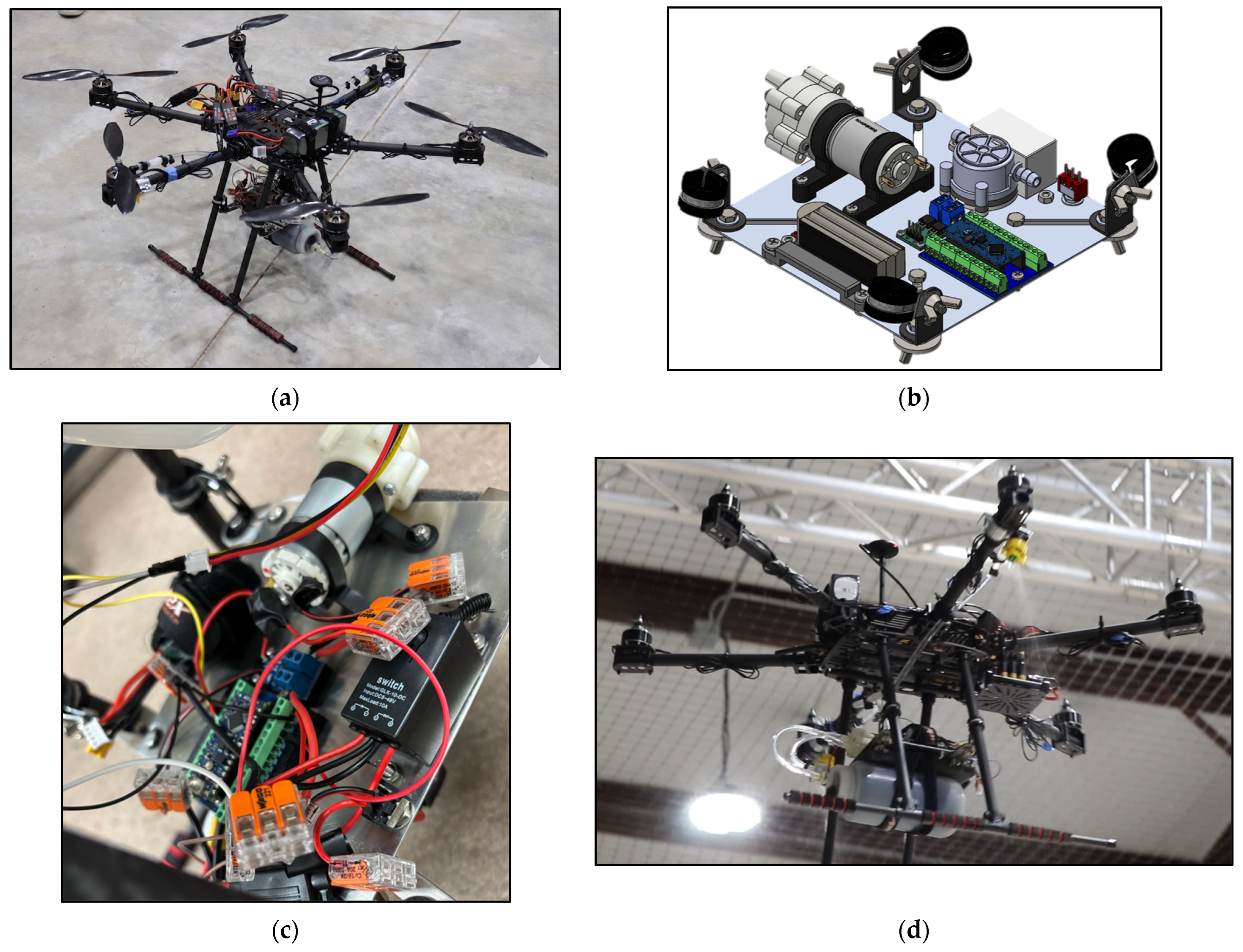
The modular spray system is designed with three primary goals: modularity, lightweight construction, and adjustable nozzle configuration. These design objectives are selected to ensure compatibility with small UAV platforms while maintaining flexibility for experimental evaluation. Modularity allows rapid swapping of tanks, nozzles, and batteries, enabling efficient testing of multiple configurations without structural redesign. Lightweight construction is critical due to UAV payload limitations. Reducing system mass improves flight endurance, maintains a stable center of gravity, and minimizes adverse effects on maneuverability. Adjustable nozzle placement allows variation in number, spacing, and orientation, which is essential for validating CFD-predicted configurations. Additional design considerations include cost, manufacturability, and operational safety. Commercial off-the-shelf components were prioritized to reduce fabrication complexity and improve reproducibility. The system is designed for easy assembly and maintenance in typical workshop conditions while ensuring consistent spray performance and safe operation. An overview of the complete system is shown in Figure 4.

The mechanical layout is developed through iterative CAD modeling and is refined during assembly. The final configuration uses a 1 L HDPE tank mounted beneath a 6″ × 6″ aluminum plate, with the pump, flow sensor, electronics, and battery mounted above, as illustrated in Figure 4b. This arrangement provides a compact footprint and maintains a balanced mass distribution relative to the UAV frame. The mounting system uses slotted braces and clamps to accommodate different hexacopter geometries and allows removal as a single module. The integrated electronics and wiring layout is shown in Figure 4c, highlighting the compact placement of control hardware. During design, nozzle placement initially follows CFD predictions, with nozzles mounted on the front arms. However, this configuration shifts the center of gravity forward. To maintain stability, the final system places the nozzles on the center arms, providing improved mass balance during flight, as seen in Figure 4d.

The fluidic system consists of the HDPE tank, diaphragm pump, inline flow sensor, and nozzle assemblies. Foam inserts within the tank reduce fluid sloshing, and a vent prevents vacuum formation. A diaphragm pump was selected due to its lower mass and ability to maintain consistent flow under varying operating conditions. Flow rate is monitored using a Hall-effect sensor (ALLECIN E.C. US, Shanghai, China) and controlled via a microcontroller to maintain a target application rate. This closed-loop control ensures consistent spray output during operation. An Arduino microcontroller (DIYables, Republic of Korea) was programmed to regulate the automated spraying system by measuring the liquid flow rate and adjusting the pump to maintain the desired flow. A flow sensor counts pulses proportional to the fluid flow, and every 200 ms, the program converts the pulses calculated into a flow rate using the manufacturer-provided calibration constant, where the K factor was adjusted by 8% after multiple calibration trials (Equation (13)) [33].

$$F=\left(98\times 1.08\right)\times Q$$

(13)

A PI controller continuously compares the measured flow rate against the target value of 0.8 L/min and adjusts the pump speed via a MOSFET (Ceksezx Direct, China) using PWM to minimize the error between the measured and target flow rates. The program also tracks the cumulative volume dispensed and uses an automatic shutoff function that deactivates the pump when the measured pulse frequency drops below a defined threshold while the pump is operating at high output, indicating that the tank has been emptied. System activation and deactivation were controlled wirelessly using a digital high/low signal from a remote switch. The nozzle mounts are fully adjustable, allowing variation in nozzle number, spacing, and orientation without modifying the core structure. This modular design enables systematic evaluation of different spray configurations and supports direct comparison with CFD predictions. The total system mass, including payload, was approximately 1.8 kg, corresponding to 40% of the UAV payload capacity, with a controlled flow rate of 0.8 L/min during operation.

2.8. Experimental Validation Setup

Prior to field testing, a preliminary bench validation of the spray system was conducted to verify the proper functionality of the electronics, pump, and nozzle connections before mounting the system to the hexacopter. This test was also used to refine the control system and confirm reliable wireless activation of the pump. A flow rate symmetry test was also performed by placing collection containers under each nozzle and recording the discharge over time. The mass of liquid (water) collected was measured using a digital scale, confirming that the system delivered nearly equal flow rates across both nozzles. This ensured that any differences observed during flight testing were due to aerodynamic effects rather than hardware inconsistencies.

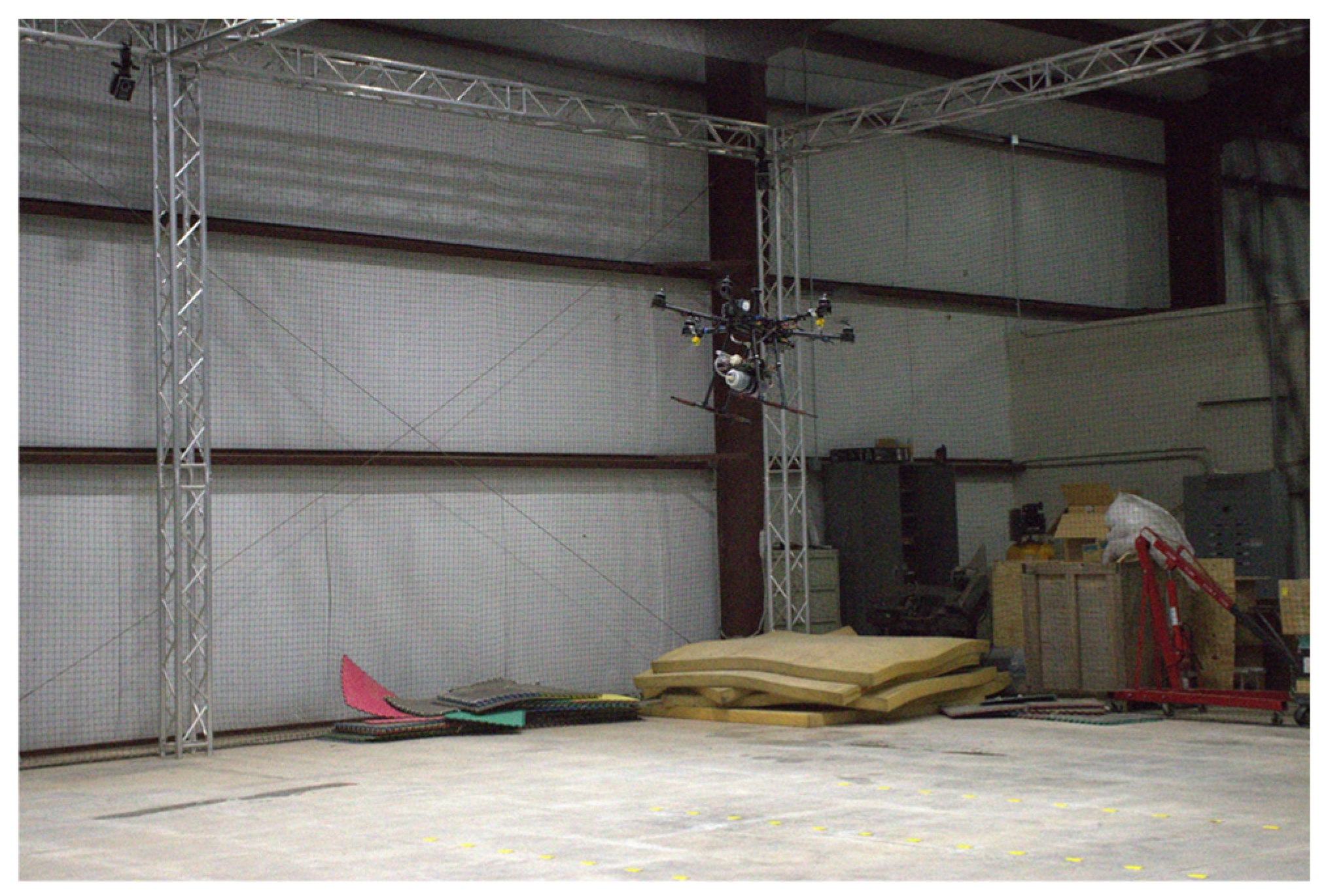
Following component-level validation, experimental testing of the complete UAV spray system was conducted indoors at the University of Oklahoma Drone Dome, as shown in Figure 5. Pure water was used as the working fluid throughout all experiments to maintain consistency with CFD assumptions. Ambient conditions remained relatively stable throughout testing due to the controlled indoor environment. Indoor testing was selected to eliminate environmental effects such as wind and temperature variation, allowing a controlled comparison with CFD predictions. Validation through field testing will be necessary for future developments of this technology, as it would provide a more accurate representation of how the UAV and attached systems would behave during commercial applications. Additionally, it would also have the benefit of potentially identifying unforeseen interactions between the UAV and the environment that would need to be addressed in future iterations. For the work done in this study, it was decided that establishing a performance baseline easily comparable to numerical data was a priority, which contributed to the decision to use indoor testing, alongside the fact that we had more connections that would allow us to coordinate the use of an indoor space. Spray deposition was quantified using water-sensitive paper (WSP), which changes color upon droplet impact and allows measurement of droplet distribution and coverage.

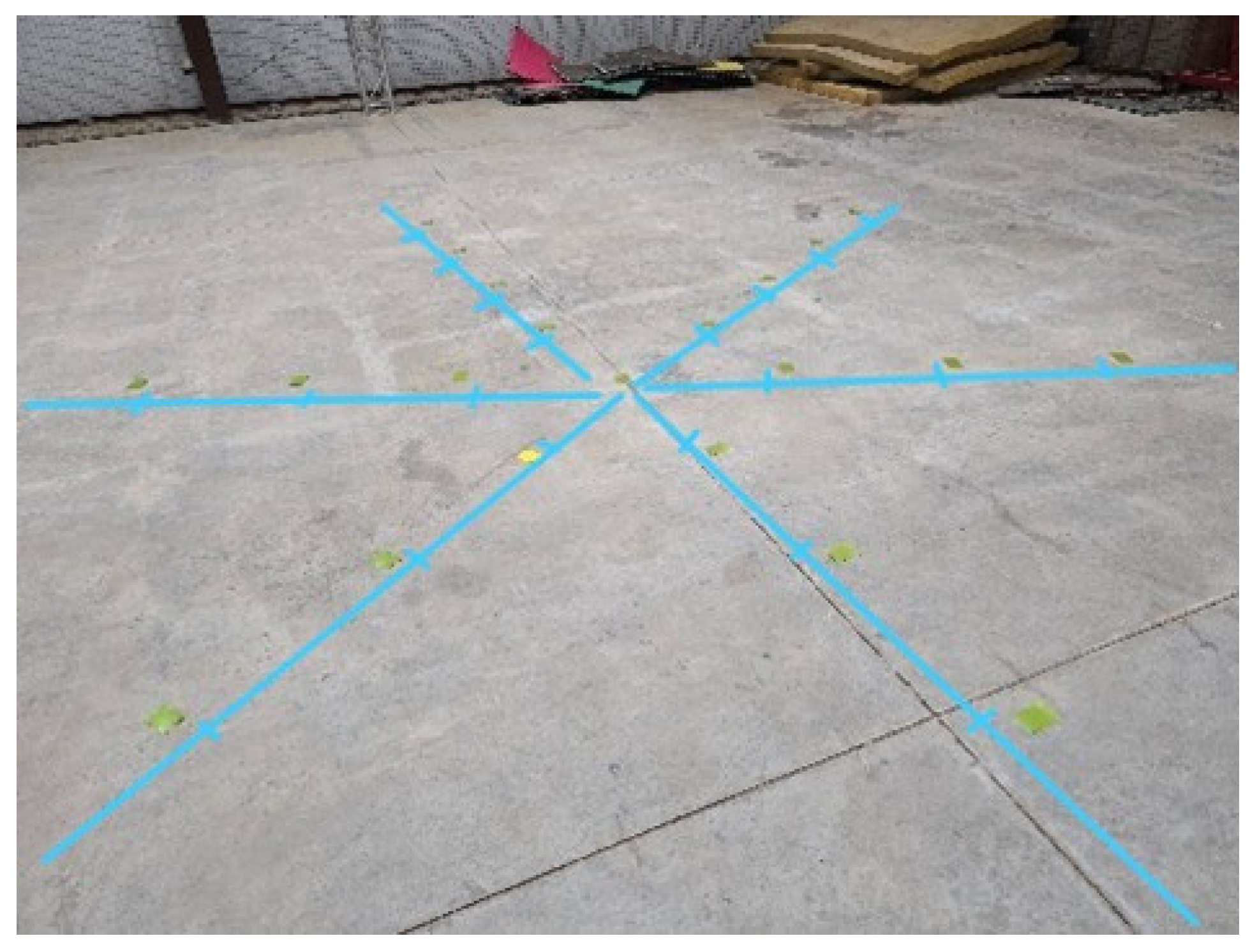
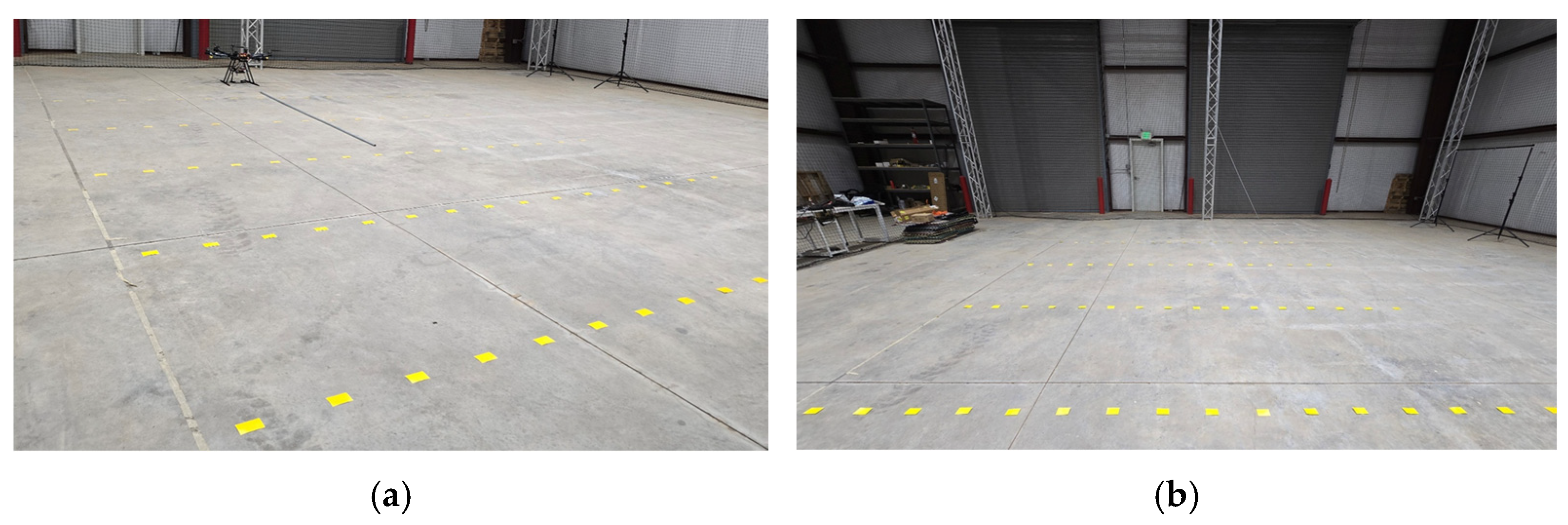
Two stationary hover tests and two forward-flight tests were conducted to evaluate spray behavior under different operating conditions. In the hover tests, WSP cards were arranged in a radial pattern centered at the UAV position, as illustrated in Figure 6. A total of 25 cards were placed along six radial directions at 60° intervals, with multiple distances from the origin to capture deposition variation. The UAV was positioned at an approximate altitude of 2 m, and the spray system was activated for a short duration. Due to the lack of GPS stabilization in the indoor environment, maintaining a perfectly stationary hover required continuous pilot correction, resulting in slight drift during testing. Forward-flight tests were conducted using a grid-based layout of WSP cards arranged perpendicular to the flight path, as shown in Figure 7. The grid consisted of multiple rows spaced along the direction of travel, with uniform lateral spacing within each row. The UAV was flown along the centerline of the grid at a target altitude of approximately 2 m and a nominal forward velocity of 2 m/s, although variations occurred due to manual control. The spray system was activated prior to entering the grid and deactivated after passing the final row to ensure full coverage. Special care was taken in handling and processing the WSP cards to maintain data accuracy. Cards were handled using gloves to prevent contamination and were left undisturbed after spraying to allow complete absorption of droplets. Each card was labeled and stored systematically to avoid mixing or cross-contamination.

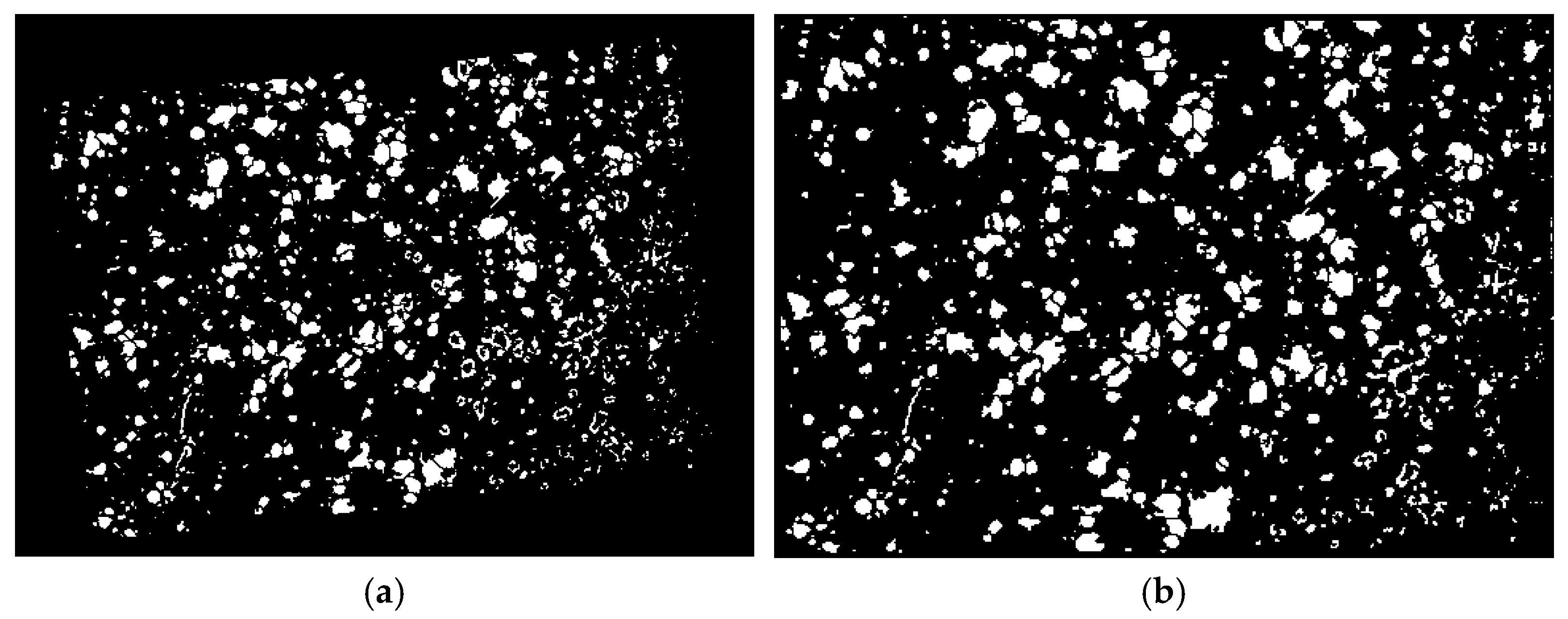
Image processing of the WSP cards was performed using Fiji (ImageJ 2.9). Multiple cards were captured per image and analyzed using defined regions of interest (ROI). All images were calibrated based on known WSP dimensions to ensure consistent scaling. Images were converted to grayscale and thresholded to separate droplet marks from the background. Additional processing steps included hole filling and watershed segmentation to separate overlapping droplets, as illustrated in Figure 8a,b. In some cases, variations in lighting required manual adjustment of threshold values to ensure accurate droplet identification.

Droplet characteristics were quantified using particle analysis tools within Fiji, which provided both individual droplet measurements and summary statistics. Four primary metrics were evaluated. The first was the volume median diameter (DV50), defined as the droplet diameter at which 50% of the spray volume is contained in smaller droplets, as described by ASABE Standard S327.4 [34]. This metric was used to assess droplet atomization and identify potential secondary breakup effects [35]. The second metric was the effective swath width, determined using the 50% maximum deposition criterion following ASABE Standard S341.3 [36]. This metric represents the usable spray width where sufficient coverage is achieved and is critical for evaluating application efficiency [37]. The third metric was the percentage area coverage obtained from the WSP analysis, which provides a measure of droplet deposition density. Finally, spray uniformity was evaluated using the coefficient of variation (CV%), calculated over the effective swath width [38]. Lower CV% values indicate more uniform spray distribution, which is generally desirable in agricultural applications.

The experimental results showed trends consistent with CFD predictions, particularly in terms of spray distribution patterns and relative performance of nozzle configurations. However, discrepancies were observed in droplet size and uniformity. These differences are primarily attributed to limitations in experimental conditions, including UAV drift due to manual control, variability in flight speed, and sensitivity of image processing to lighting conditions.

3. CFD Results

3.1. Baseline Downwash (No Spray)

The initial simulation was conducted using only actuator disks to establish a baseline for rotor-induced airflow without spray injection. The resulting flow field is shown in Figure 9, where the maximum velocity magnitude reaches approximately 16.8 m/s. High-velocity regions persist near the rotor cores and extend toward the ground plane, with velocities remaining above 13.4 m/s within 0.5 m of the ground. The downwash jets generated by each rotor remain largely distinct, exhibiting minimal interaction in the upper region of the domain. As the flow approaches the ground plane, slight convergence occurs before the jets diverge laterally.

This behavior is consistent with prior studies [17], which report distinct rotor jets that retain high velocity near the rotor exit and gradually interact closer to the ground. Minor differences in velocity magnitude and flow structure are expected due to differences in rotor configuration, aircraft geometry, and the absence of forward motion in the present study.

3.2. Flow Fields Across Configurations (C1–C6)

The velocity contours and pathlines for the four boom configurations are presented in Figure 10. Across all configurations, the overall flow structure remains similar to the baseline case, with only minor reductions in peak velocity (approximately 16.5 m/s). The presence of spray injections introduces localized disturbances in the flow field, causing earlier interaction and merging of rotor jets. However, variations in nozzle spacing and number do not significantly alter the global flow structure. This indicates that spray injection has a measurable but limited influence on the overall downwash characteristics.

Similarly, the under-rotor configurations shown in Figure 11 exhibit nearly identical flow structures, with peak velocities also reaching approximately 16.5 m/s. The flow slows to approximately 10 m/s near the ground due to interaction with the no-slip boundary. Overall, these results suggest that while the presence of a spray affects local flow behavior, the dominant flow characteristics are governed primarily by rotor-induced downwash rather than nozzle configuration.

3.3. Particle Trajectories and Velocity Behavior

The particle trajectories for all configurations are shown in Figure 12 and Figure 13. In all cases, spray particles initially follow the expected fan-shaped distribution but rapidly decelerate due to drag and interaction with the surrounding airflow. Particles that enter the high-velocity rotor jets experience strong downward acceleration and follow steep trajectories toward the ground. In contrast, particles outside these jet regions lose velocity more quickly and drift outward due to lateral flow divergence near the ground.

For boom configuration one, the central nozzle produces a relatively narrow deposition pattern, as most particles remain within the rotor influence zone and are directed downward before significant lateral spread occurs. In boom configuration two, the addition of side nozzles increases the deposition area. Particles originating from outer nozzles experience less interaction with the rotor core flow, allowing for greater lateral dispersion. This leads to a wider but less concentrated deposition pattern. Boom configurations three and four show similar behavior, with configuration four exhibiting slightly higher particle velocities due to its closer proximity to rotor jets. This results in reduced drift compared to configurations two and three while maintaining relatively wide coverage.

For the under-rotor configurations (Figure 13), particles are introduced directly within the rotor downwash, resulting in higher particle velocities (up to 17 m/s). Under-rotor configuration one directs particles more uniformly downward, while configuration two exhibits a slight directional bias due to nozzle placement. Overall, under-rotor configurations reduce drift and increase deposition concentration due to stronger coupling with rotor-induced airflow.

3.4. Deposition Footprints

The deposition areas of the different configurations are qualitatively evaluated through approximating the total area containing the sprayed particles on the map of the ground plane, as shown in Figure 14 and

Table 4. Sprayer configuration estimated deposition areas.

	Length (m)	Width (m)	Area (m2)
Boom Configuration One	5.046	1.789	9.027
Boom Configuration Two	8.310	4.437	36.868
Boom Configuration Three	8.382	4.485	37.597
Boom Configuration Four	7.857	4.214	33.112
Under-Rotor Configuration One	8.077	3.846	31.065
Under-Rotor Configuration Two	9.286	3.571	33.163

.

Boom configuration one produces the smallest deposition area (approximately 9.027 m²), with a narrow and concentrated pattern. Configurations two and three achieve the largest coverage areas (approximately 36–38 m²), primarily due to increased lateral dispersion from multiple nozzles. Boom configuration four provides a balance between area and concentration, with a deposition area of approximately 33.112 m².

Under-rotor configurations produce slightly smaller deposition areas (approximately 31–33 m²) but exhibit improved central concentration. Configuration one, in particular, demonstrates higher particle density near the center of the deposition zone. These results indicate that increasing the nozzle number increases coverage area but often reduces deposition density and uniformity due to enhanced droplet dispersion.

3.5. Quantitative Deposition Evaluation

Quantitative metrics for selected configurations are presented in

Table 5. Sprayer evaluation metrics final values.

	Effective Deposition Area (m2)	Effective Application Rate (mL/m2)	Coefficient of Variation (%)
Boom Configuration Four	10.585	0.03377	52.30
Under-Rotor Configuration One	9.375	0.03886	45.25
Under-Rotor Configuration Two	10.222	0.03589	52.90

. These include effective deposition area, effective application rate, and coefficient of variation (CV%).

Boom configuration four exhibits an effective deposition area of 10.585 m² with a CV% of 52.30, indicating moderate uniformity. Under-rotor configuration one achieves the lowest CV% (45.25), indicating improved uniformity, along with the highest effective application rate (0.03886 mL/m²). Under-rotor configuration two shows slightly higher variability (CV% = 52.90), which is attributed to uneven distribution across the deposition region.

Under-rotor configuration one demonstrates the best overall performance among the evaluated setups. Compared with Boom Configuration Four (CV% = 52.30), it reduced the coefficient of variation to 45.25%, representing an improvement in spray uniformity of approximately 13.5%. Additionally, it achieved the highest effective application rate (0.03886 mL/m²), indicating a favorable balance between deposition concentration and uniformity. The lower CV% indicates improved deposition uniformity, which is consistent with findings from previous studies [20]. Although this configuration provides a slightly reduced deposition area compared to boom configurations, it delivers a higher and more uniform application rate across the target region. Despite its favorable performance, under-rotor configuration two was selected for experimental testing due to improved mass distribution and reduced impact on the UAV’s center of gravity.

3.6. Sensitivity Analysis

A sensitivity analysis is conducted for under-rotor configuration one to evaluate the influence of key parameters on simulation outcomes. The changed variables include droplet diameter, which is varied by ±20%, and operational altitude, which is varied by ±0.5 m. These parameters are chosen because they are the most likely to have unintended discrepancies between the simulated and experimental setups. The results of these new simulations are displayed in

Table 6. Altitude and Droplet Size Sensitivity Results.

	Effective Deposition Area (m2)	Effective Application Rate (mL/m2)	Coefficient of Variation (%)
Under-Rotor Configuration One Original	9.375	0.03886	45.25
Altitude 0.5 m Increase	11.450	0.02983	42.19
Altitude 0.5 m Decrease	7.526	0.05419	45.26
Droplet 20% Increase	7.774	0.04569	38.09
Droplet 20% Decrease	11.047	0.03637	51.87

below.

The trends displayed by the results suggest that while the two parameters have a similar impact on deposition area, altitude has a larger impact on effective application rate while influencing CV% more. A higher altitude increases drift potential, aligning with behaviors seen in previously analyzed particle tracks, but also appears to improve uniformity. This is possibly a result of the increased amount of drift, giving the droplets a proper amount of time to be distributed more evenly throughout a larger area, which is why the application rate decreases. The same analysis can then be applied to the decreased altitude condition, which demonstrates how the reduced drift potential can improve application rate but likely causes the fluid to pool underneath the nozzles, increasing CV% and decreasing deposition area. Notably, the increase in CV% is marginal compared to other value changes. This likely means that uniformity is not subject to change very much as a result of relatively small decreases in altitude.

An increase in droplet size, and therefore mass, results in the droplets having more inertia and, therefore, reduced drift potential. Despite this, CV% decreases with this smaller potential for drift, as opposed to when altitude changes, where it increases slightly with reduced drift potential. The increased inertia most likely prevents the droplets from reaching the exterior of the rotor downwash jets, as they are injected with a primarily downward trajectory while the downwash maintains it, and the particles are better suited to maintain that trajectory. Therefore, fewer particles have the potential to drift, as they do not reach the exterior of the downwash jets, decreasing the deposition area but improving uniformity and application rate within that area.

Sensitivity results overall indicate that droplet size has a significant impact on deposition behavior, particularly on uniformity. Conversely, changes in altitude have a larger impact on effective application rate due to the amount of drift allotted by the altitude, increasing or decreasing the deposition area. Notably, a relatively small variety of values was used during this sensitivity analysis. Testing additional cases would be necessary in future work to get a clearer understanding of how these parameters would affect the numerical results.

3.7. Comparison with Prior Studies

Simulation results were compared with literature data [17] using volumetric flow rate distributions (Figure 15). The present simulations show peak deposition concentrated near the centerline due to overlapping spray patterns, whereas the referenced study shows dual peaks corresponding to a single nozzle under one rotor.

Differences are attributed to variations in nozzle configuration, droplet size, and operating height. Despite these differences, the overall trends in deposition behavior are consistent, supporting the validity of the current model.

4. Experimental Validation

4.1. Ground Results

As shown in

Table 7. Ground Testing Results.

Trial	Time-to-Empty (s)	Left Nozzle (L)	Right Nozzle (L)	Combined (L)
1	73	0.322	0.318	0.640
2	70	0.310	0.307	0.617
3	73	0.314	0.309	0.623
AVG	72	0.315	0.311	0.627

, the average usable liquid capacity of the system was approximately 0.627 L. Although a 1 L HDPE bottle was used, the effective capacity was reduced due to the presence of internal tubing and foam inserts, which occupy volume and retain a portion of the fluid during operation. The results also demonstrate that the system distributes flow evenly between the two nozzles, with approximately 50.3% delivered to the left nozzle and 49.7% to the right. This near-equal distribution confirms that the flow system is well balanced and that any differences observed in spray deposition are primarily due to aerodynamic effects rather than hardware inconsistencies. Using the average discharge time and measured capacity, the mean flow rate of the system was calculated to be approximately 0.523 L/min, indicating stable and repeatable fluid delivery under ground-testing conditions.

4.2. Flying Results

Table 8. Hover Test Results.

Trial	Avg. DV50 Size (µm)	Swath Width at 2 m Height (m)	Avg. Area Covered (%)
1	531	2.8 *	1.3
2	705	1.8	1.7
AVG	618	1.8	1.5

* Larger width attributed to card spacing and is neglected.

presents the results obtained from stationary hover tests. The average droplet size (DV50) was calculated to be approximately 618 µm, indicating relatively coarse droplets compared to the CFD assumptions. There were several reasons for the discrepancy between the numerical and experimental droplet diameters. The first was the changes in the sprayer system design when moving from the conceptual design phase, which is what primarily informed the numerical setup. Though the brand of nozzle was the same as the one used as the basis for the simulations, the model was different and therefore had a different expected droplet diameter. However, what likely had a greater influence on experimental values was the method of data collection. The water droplets likely coalesced as they contacted the paper and then expanded as they were absorbed into it. While steps were taken to break up large apparent droplets on the card samples using the analysis program, there was an intention to do so minimally so as not to significantly tamper with the data. Therefore, the measured DV50 values should be interpreted as estimates of deposited droplet characteristics rather than direct measurements of droplet diameters at the nozzle exit. The effective swath width was determined to be approximately 1.8 m. Although Trial 1 produced a larger apparent swath width (2.8 m), this value resulted from increased spacing between WSP cards and is therefore not considered representative. The second trial, which employed closer spacing, provides a more accurate estimate of system performance. The average area coverage within the swath was approximately 1.5%, indicating an ultra-low-volume spray regime. This level of coverage suggests that the spray system is operating in a targeted application mode, rather than delivering dense, uniform saturation across the entire swath.

As shown above in

Table 9. Flying Test Results.

Trial	Avg. DV50 Size (µm)	Swath Width at 2 m Height (m)	Avg. Area Covered (%)	Coefficient of Variation (%)
1	530	1.7	1.1	27.5
2	474	1.8	0.6	45.5
AVG	502	1.8	0.8	36.5

, the flying test results exhibit trends similar to those observed during hover testing, with some notable differences. The average droplet diameter in flight conditions was smaller, with a DV50 of approximately 502 µm, suggesting increased atomization or breakup due to airflow interactions during motion. The average swath width remained consistent at approximately 1.8 m, indicating that forward motion had minimal impact on overall coverage width. However, the average area coverage decreased to 0.8%, reflecting increased dispersion of droplets during flight. The coefficient of variation (CV%) within the effective swath was calculated to be 36.5%, indicating moderate uniformity. Trial-to-trial variability was observed, with CV% ranging from 27.5% to 45.5%, highlighting the influence of manual flight control and varying operating conditions. One limitation of this study was the small number of trials conducted for both the hover and flight testing. The limited trials were mainly due to constraints related to access to the testing space and time restrictions. Additionally, unexpected complications, such as technical difficulties, caused some trials to be delayed, resulting in a total number that was fewer than initially planned. Consequently, the calculated averages are less representative of the trends observed in the experiments. To address this issue, additional trials should be conducted in future iterations of this work.

4.3. Metric Comparison

When compared to CFD predictions, several key differences are observed. The experimentally measured droplet diameter (≈502 µm) is significantly larger than the simulated value (~280 µm), indicating that the modeling assumptions may underestimate droplet size or secondary coalescence effects. The measured swath width of 1.8 m is reasonably close to the CFD-predicted effective swath of approximately 2.0 m, suggesting good agreement in overall spray coverage behavior. However, the experimental uniformity (CV% = 36.5%) is noticeably better than the variation predicted in CFD simulations for the under-rotor configurations (CV% = 45.25–52.90%), with a difference of approximately 12.6%. Agreement between CFD and experimental measurements varied depending on the metric considered. Swath width differed by approximately 10%, while significantly larger discrepancies were observed for droplet-size measurements. These findings indicate that the CFD model more accurately captured overall deposition behavior and coverage trends than absolute droplet-size characteristics.

5. Discussion

5.1. Mechanistic Interpretation

This research provides insight into how sprayer nozzle positioning influences system performance when integrated into an agricultural UAV. Comparisons between simulated flow velocity profiles and pathlines across configurations provide the basis for the prediction that the presence of spray injection beneath a rotor does influence the local behavior of rotor-induced downwash. However, the overall structure of the downwash remains largely similar between configurations, suggesting that nozzle placement does not significantly alter the global airflow field. Analysis of fluid particle trajectories demonstrates how downwash subsequently affects droplet motion. In general, particles initially disperse outward from the nozzle and move toward the ground plane. As they interact with rotor-induced airflow, their trajectories become strongly influenced by local velocity fields. Particles entering high-velocity rotor jets are rapidly accelerated downward, while those outside these regions experience greater lateral drift. While the global airflow field is not significantly changed by the position of the nozzles, meaning the location of these local velocity fields is relatively consistent, the position of the nozzles relative to them changes. This changes how fluid droplets interact with the fields due to the differences in trajectory and velocity, and is likely why the nozzle position can have such a pronounced effect on the fluid deposition while leaving the airflow field relatively unchanged.

These simulation results indicate that nozzle placement relative to rotor flow has a direct effect on deposition patterns. Positioning nozzles beneath or between rotors reduces lateral drift and concentrates deposition within a smaller region, resulting in increased density and improved uniformity. For example, Under-Rotor Configuration One achieved a coefficient of variation of 45.25%, compared with 52.30% for Boom Configuration Four, representing an improvement in uniformity of approximately 13.5%. The analysis of the simulated deposition maps indicates that increasing the number of nozzles does not significantly impact the performance of individual nozzles; instead, it enhances the overall coverage area. Introducing a second nozzle typically improves performance by increasing both density and uniformity. However, adding further nozzles tends to primarily expand the deposition area, which could lead to a decrease in uniformity if the spacing between nozzles becomes excessive. It is important to note that these observations stem from numerical findings and necessitate further experimental validation with additional configurations.

A key observation from both simulation and experimental results is that effective application rate and uniformity tend to be inversely related to deposition area. Configurations that produce wider coverage often exhibit lower uniformity and reduced deposition density, whereas more concentrated configurations yield higher application rates and more consistent coverage. These findings are supported by experimental results, which display similar trends in deposition behavior despite variability in flight conditions. While further testing is required to fully validate these relationships, the current results provide consistent evidence supporting the conclusions drawn from the CFD simulations.

5.2. Agronomic Implications

While this study identifies high uniformity and deposition density as desirable performance characteristics, these outcomes may not be optimal for all agricultural applications. Different crops and treatment strategies require varying levels of coverage, droplet size, and application rate. This highlights a key limitation of the study, as the results are based on a small-scale UAV platform and a specific set of operating conditions. In larger-scale agricultural operations, tradeoffs between coverage area and concentration may be prioritized differently depending on crop type, field size, and economic considerations.

For example, in some applications, maximizing coverage area may be more beneficial than achieving high local concentration, particularly where uniform distribution over a wide region is required. Conversely, targeted applications may benefit from the concentrated deposition observed in under-rotor configurations. As a result, further research is needed to evaluate how these findings translate to commercial-scale systems and to determine optimal configurations for different crop and application scenarios. The relatively low coverage values observed experimentally (0.8–1.5%) are characteristic of ultra-low-volume applications and reflect the coarse droplet spectrum evaluated in this study. Consequently, the results should be interpreted primarily as demonstrating the influence of nozzle placement on deposition behavior rather than as a direct assessment of pesticide efficacy.

5.3. Engineering Implications

From an engineering perspective, the results suggest that placing nozzles directly beneath the rotors is advantageous due to reduced droplet drift and increased interaction with downward airflow. This configuration leads to improved deposition uniformity and application efficiency, although it results in a slight reduction in total coverage area. Nozzle spacing is also identified as a critical design parameter. Excessive spacing between nozzles can lead to reduced uniformity and lower deposition density in intermediate regions, while overly compact spacing increases system weight and fluid usage without significant performance benefits.

Based on the configurations evaluated in this study, an effective nozzle spacing is estimated to lie between approximately 0.375 m and 0.75 m. This is shown by the selected C5 and C6 configurations and aligns well with the 0.6 m value provided by [20], which was used as a reference when determining the sprayer system characteristics. However, this range is derived from a limited set of test cases and should be considered a preliminary guideline rather than a definitive design rule. These findings suggest that optimal UAV spray system design requires balancing competing factors, including coverage area, uniformity, payload capacity, and system complexity.

5.4. Integration into Field Operations

The results of this study demonstrate that CFD is a valuable tool in the design and optimization of agricultural UAV spray systems. By enabling rapid evaluation of multiple configurations, CFD allows designers to identify promising system architectures prior to physical testing, reducing development time and cost. There is a consensus regarding the relative performance trends observed across different configurations; however, notable discrepancies exist between certain values derived from numerical data and experimental results that warrant attention. One such value is the average droplet diameter, which highlights the necessity for validation when employing this approach. Nonetheless, the capacity to replicate experimental trends underscores the approach’s utility.

This methodology is especially relevant for variable-rate spraying applications, where spray parameters must be adjusted dynamically to match crop requirements. CFD-based modeling can help predict how changes in nozzle configuration, operating conditions, and UAV design affect spray deposition, allowing for more precise and efficient application strategies. Practical deployment of UAV spray systems will also depend on factors not explicitly considered in this study, including ambient wind conditions, crop canopy architecture, refill logistics, battery endurance constraints, and regulatory requirements associated with aerial pesticide applications. By integrating CFD analysis with practical experimental validation, this study provides a framework for developing more efficient, adaptable, and application-specific UAV spraying systems.

6. Conclusions

The research conducted in this study illustrates how key sprayer system design parameters influence spray performance in an agricultural hexacopter and demonstrates the capability of CFD to inform UAV spray system design. This was achieved through analysis of the interaction between sprayed droplets and rotor-induced downwash, with results supported by both a mesh independence study and experimental validation. The simulation results indicate that nozzle placement relative to the rotors significantly impacts deposition behavior, particularly in terms of deposition area and particle density. These effects arise primarily from the influence of downwash on droplet trajectories. Under-rotor configurations were shown to be more favorable in this study, as the downward-directed airflow enhances deposition concentration and reduces lateral drift. Among the evaluated configurations, Under-Rotor Configuration One produced the highest effective application rate (0.03886 mL/m²) and the lowest coefficient of variation (45.25%), representing approximately a 13.5% improvement in uniformity over the best-performing boom configuration. This configuration yielded experimental results indicating a droplet size of 502 µm, a swath width of 1.8 m, an area coverage of 0.8%, and a coefficient of variation of 36.5%. In contrast, nozzles positioned near the edges or between the rotors showed enhanced droplet dispersion but limited effective spread. The number of nozzles was found to have a less direct impact on performance compared to placement, although increasing nozzle count naturally increases total coverage area. However, gains in coverage may come at the expense of uniformity if spacing is not properly optimized.

The results also suggest that the relative advantage of under-rotor configurations is influenced by the smaller scale of the UAV platform used in this study. Under-rotor setups inherently limit nozzle spacing and number, making them more suitable for applications requiring concentrated and uniform deposition. In contrast, boom configurations may be more appropriate for applications where maximizing coverage area is the primary objective. Overall, this study demonstrates that CFD-informed design provides a useful first-order approximation for optimizing UAV spray systems, provided that key parameters such as droplet size are calibrated against experimental measurements.

Several areas of improvement for this work have been identified that could potentially allow this approach to accurately capture complex interactions, as opposed to serving as an approximation. One primary limitation is the inconsistency between the UAV configuration used in the simulations and the final experimental system. Although the simulations were developed with a degree of generalization to accommodate design changes, improved agreement between numerical and experimental results could be achieved by updating the CFD model to more closely match the as-built system. Experimental uncertainty can also be reduced through improved testing methods. A major source of variability in this study was pilot-induced error, particularly due to the lack of GPS-assisted stabilization in the indoor testing environment. Future work should incorporate automated flight control, allowing for more consistent flight paths, stable altitude control, and improved repeatability of results.

Further experimental validation should include patternator testing to obtain more precise and continuous measurements of spray deposition. In addition, outdoor field testing would allow for evaluation under realistic operating conditions, including the use of GPS-assisted flight and the influence of environmental factors such as wind. Advancing the numerical modeling approach is also an important next step. Future simulations should incorporate additional physical effects such as canopy interaction, forward flight motion, and potentially droplet breakup or evaporation. These enhancements would improve the accuracy of predictions under real-world conditions. Finally, further work should investigate how the conclusions of this study scale to larger UAV platforms and commercial agricultural applications. Evaluating system performance at larger scales will be essential for determining the broader applicability of the findings and for translating CFD-informed design principles into practical deployment strategies.