A Bayesian Optimization-Based AUV Swarm Model in a Double-Gyre Flow Field

Highlights

What are the main findings?

• A behavior-based swarm control architecture is proposed for coordinated motion in time-varying Double-Gyre flow fields, where a graph attention mechanism guided by agent heading angles dynamically assigns inter-agent interaction weights.
• A Bayesian optimization framework is introduced to determine the optimal behavioral weights for swarm coordination.

What are the implications of the main findings?

• This method enhances swarm adaptability, coordination stability, and control performance under complex environmental disturbances.
• The framework provides a robust and scalable basis for swarm control in dynamic flow environments, with promising potential for autonomous marine multi-agent applications.

Abstract

Conventional cooperative control methods for multi-AUV systems typically rely on quasi-steady hydrodynamic assumptions and do not explicitly account for time-varying uncertainties in ocean dynamics. In addition, controller parameters are often tuned empirically. As a result, under complex disturbed flow fields and communication constraints, AUV swarms are prone to group fragmentation and reduced polarization, which undermines stable cooperative navigation. To address these limitations, we propose a double-gyre-flow-optimized autonomous underwater vehicle swarm (DGF-OAS) model for coordinated operations in time-varying flow fields. The proposed model incorporates a heading-aware graph attention mechanism to adaptively adjust adjacency weights among agents with different roles. It further integrates the Lennard–Jones potential to preserve safe inter-vehicle spacing and embeds a periodically varying double-gyre flow field to characterize ocean disturbances. Bayesian optimization is then employed to automatically identify suitable weights for the alignment and attraction–repulsion terms, thereby improving swarm cohesion and environmental adaptability. Simulation results demonstrate that, under flow-field disturbances, DGF-OAS achieves group polarization of up to 96%, reduces the average task completion time by 15.84% compared with the baseline model, and attains a task completion rate of 97%, significantly outperforming the compared methods. These findings indicate that the proposed approach exhibits strong adaptability and stability in complex environments and offers an effective solution for AUV swarm control.

1. Introduction

Autonomous underwater vehicles have become an important enabling technology in marine engineering, driven by the growing demand for underwater operations, ocean resource exploitation, and marine ecological protection [1,2,3]. Compared with single-vehicle systems, multi-AUV swarms offer higher operational efficiency and stronger environmental adaptability, delivering pronounced advantages in complex mission scenarios [4]. Classical strategies for multi-robot swarm control include the leader–follower paradigm [5], the virtual structure method [6], and behavior-based control [7]. More recently, deep reinforcement learning has attracted increasing attention in multi-agent cooperative control [8,9]. Among these, behavior-based control is inspired by the emergent phenomena of natural collectives such as fish schools and bird flocks [10,11]. Through purely local interactions, agents self-organize their motion by enforcing short-range repulsion, mid-range alignment, and long-range attraction. The approach is decentralized, self-organizing, and robust. It is now well established in aerial and ground swarm robotics. However, in complex underwater environments, its performance is susceptible to strong currents and measurement noise and is further challenged by communication constraints.

In traditional underwater swarm control, AUVs are often modeled as particles while environmental disturbances are approximated as stochastic noise. Yet in realistic current fields, the flow exerts a pronounced influence on individual trajectories and collective coordination and can even cause severe performance degradation. To account for background flows, prior work that assumes full knowledge of the flow field has investigated cooperative path optimization and trajectory planning for multiple AUVs [12,13,14]. In practice, however, complete flow information is generally unavailable. To reduce reliance on global flow data, some studies enable navigation from purely local sensing without prior environmental knowledge [15,16]. These methods, though effective, are limited to single-agent settings and typically require large quantities of current data for training. Beyond single-agent navigation, other works fuse local observations to realize multi-AUV cooperative control under flow-field conditions [17] and propose swarm control tailored to regimes with strong currents [18]. Nevertheless, the periodic nature of ocean flows continuously injects heading noise into the system, substantially weakening inter-agent alignment. In addition, flow uncertainty induces switching of the interaction topology at high frequency, which can trigger communication link breakages. This, thereby, diminishes group cohesion and increases the risk of swarm fragmentation.

Moreover, the complexity of the marine environment not only degrades collective performance but also exacerbates the challenges of underwater communication [19]. To improve communication efficiency among agents, researchers have proposed undirected information flow topologies based on proximity interactions, as well as hybrid schemes that integrate topological structure with visual interactions to reduce communication overhead while maintaining minimal neighborhood size [20]. Because multi-robot coordination often involves balancing competing objectives, optimization algorithms are widely employed to enhance multi-AUV performance. Examples include genetic algorithms for target-point assignment [21], particle swarm optimization with multiple objectives for overall path planning while considering path length, smoothness, turning angles, and ocean-current effects [22], and hybrid approaches that combine PSO with the ELKAI solver for joint task allocation and path planning [23]. Despite these advances, conventional optimization methods often require extensive sample evaluations, struggle to balance exploration and exploitation in high-dimensional parameter spaces and are prone to local optima. As a result, challenges remain in coping with complex ocean disturbances while achieving scalability to large swarms.

To address swarm control under complex flow fields, we propose an integrated framework for cooperative control and parameter optimization of AUV swarms. Building on our prior work [24,25], we first incorporate a multi-head attention mechanism into the alignment term to dynamically distribute interaction weights and thereby reduce communication load. Second, we apply the Lennard–Jones potential as a soft constraint on inter-agent spacing, maintaining a balanced distance among neighboring AUVs and mitigating collision risk. Departing from conventional models, we explicitly incorporate a noisy double-gyre flow that varies in time into the swarm dynamics to emulate oceanic disturbances. Third, we employ Bayesian optimization to tune the behavioral weights of the alignment and attraction–repulsion terms, using the mean group polarization, mean normalized arrival time, and mean task success probability as optimization objectives, thereby enhancing robustness under background flows. Extensive simulations demonstrate that, under identical environmental conditions, the proposed model achieves superior performance over baseline methods in key metrics such as polarization and task completion rate. The major contributions of this work are given below.

1. A behavior-based swarm control model is proposed for multi-AUV cooperative navigation in complex marine environments, where a local flow field disturbance term is incorporated into the individual velocity update law to describe swarm motion under time-varying flow conditions.

2. A graph attention-based adaptive neighbor-weighting strategy is developed by exploiting heading-related features. Combined with a leader-follower hierarchical architecture, the proposed strategy enhances the guiding effect of key nodes and improves heading alignment across the swarm.

3. A Bayesian optimization-based parameter tuning framework is established to optimize the key behavioral parameters of the swarm model. The optimized parameter combination contributes to improved overall swarm performance across multiple collective behavior metrics, including polarization, average inter-individual spacing, and other related indicators.

The rest of the paper proceeds as follows. Section 2 reviews previous studies related to this topic. Section 3 formulates the multi-AUV cooperative navigation problem. Section 4 introduces the framework for swarm control. Section 5 outlines the theoretical foundation and execution of the optimization method. The setup and results of the simulation are covered in Section 6. Section 7 presents the conclusions of this study and discusses future research directions.

2. Related Work

As multi-AUV systems become increasingly capable and efficient in challenging conditions, the cooperative control and optimization of underwater swarms in flow fields have attracted growing research attention. Li et al. [26] proposed an adaptive cooperative exploration strategy for multiple AUVs based on a greedy idea, which achieves target coverage in an unknown discretized grid environment while explicitly accounting for energy and communication constraints. However, this strategy does not incorporate flow field disturbances into the model, and its applicability in realistic ocean current environments remains to be further verified. For underwater acoustic sensor networks subject to complex ocean current disturbances, one study [27] employs AUVs to assist in the prediction and repair of routing holes, thereby enhancing the reliability of communication among multiple sensor nodes. In addition, most related studies typically assume that complete flow field information is available a priori and mainly focus on cooperative mission execution and path optimization for multiple AUVs. For example, Liu et al. [12] formulated task allocation and route planning for multiple AUVs as a multiobjective optimization problem and validated the proposed method on multi-objective missions in underwater scenarios constructed from a New Zealand bathymetric data set. To mitigate premature convergence to local optima in high-dimensional settings, Sun et al. [13] developed a multiobjective optimization framework combined with a dynamic window fusion algorithm for global trajectory generation of multiple AUVs in disturbed marine flow fields. This study [14] proposed a collision-avoidance strategy for multiple AUV formations operating in ocean current environments, in which an affine transformation is used to achieve formation reconfiguration and obstacle avoidance is achieved through an improved artificial potential field scheme. Near-surface experiments further demonstrate the feasibility of this method.

Although the above studies provide effective schemes for cooperative control under known flow field conditions, the highly time-varying nature of real ocean environments and the difficulty of obtaining complete flow field information impose inherent limitations on path planning and control strategies that rely on global flow field priors. Consequently, researchers have shifted their attention toward AUV control problems under local sensing constraints. Gunnarson et al. [15] employed a deep reinforcement learning algorithm to achieve AUV navigation from an initial point to a target point, and transferred the learned policy to time-varying double gyre flow environments for testing. However, the transferred policy exhibited unsatisfactory navigation success rates across different scenarios. Building on this work, a method based on proximal policy optimization (PPO) was developed in [16], which incorporates a look-ahead state space (LASS) and a flow-field prediction network, leading to a significant improvement in the agents’ navigation success rates in flow-field environments. Although these studies rely only on local information, they do not address the problem of cooperative navigation among multiple agents. The study [18] proposed a multi-AUV cooperative control method under a strong background flow field, in which smoothed particle hydrodynamics (SPH) particles are treated as equivalent to AUVs. This method maintains overall group stability while generating approximately energy-optimal cooperative motion trajectories, thereby providing a new scheme for multi-body cooperation in flow field environments.

In a multi-AUV cooperative control framework, ocean environmental disturbances are not only a primary external factor but also give rise to underwater communication link disruptions, increased difficulty in cooperative task optimization, and conflicts among individual behaviors, all of which exert a significant impact on overall system performance. To address cooperative control in congested environments, Liang et al. [20] proposed a communication architecture that integrates adaptive dynamic interaction with a bio-inspired self-organization mechanism. In [28], the position of the swarm center is estimated and treated as a global virtual reference point, thereby ensuring connectivity across the entire group. Furthermore, Tao et al. [29] proposed an air-water cross-domain communication scheme operating in real time, in which multiple unmanned aerial vehicles equipped with hydrophones form mobile acoustic base stations to satisfy the communication requirements of multi-AUV swarms in emergency scenarios. To enable information exploration over steady or unsteady marine geomorphology without requiring global characteristic scale estimation, Nitti et al. [30] integrated metaheuristic algorithms with consensus theory and developed a cooperative swarm scheme for multi-AUV systems, which serves as both an optimization tool and a control architecture. In [23], an improved Dijkstra algorithm, particle swarm optimization-based task assignment, and ELKAI for solving sub-traveling salesman problems are employed jointly to realize shortest path planning for multiple AUVs and to shorten overall mission execution time. Zhang et al. [31] designed an age-based multi-particle swarm optimization algorithm with faster convergence and a stronger capability to escape local optima, and applied it to multi-AUV path planning under complex terrain and threat region constraints. Aiming to improve cooperative planning capability in challenging scenarios, Sun et al. [32] introduced a multiobjective, multipopulation variant of the gray wolf optimization algorithm, derived from the standard framework. By introducing a multi-population cooperation structure, a multiobjective optimization mechanism, and several refined operators, this method achieves superior performance in terms of mission duration and collision probability. Although the above studies perform optimization tailored to specific tasks, relatively little attention has been devoted to the systematic optimization of the internal parameters of the underlying control models themselves.

Given that traditional swarm models typically rely heavily on manual parameter tuning, several researchers have begun to investigate automated parameter search strategies based on intelligent optimization algorithms [33]. For example, building on the classical active elastic sheet (AES) swarming model, Bahaidarah et al. [34] incorporated a multiobjective particle swarm optimization (PSO) procedure to automatically optimize the control parameters and thereby enhance swarm polarization. In addition, training swarms to perform collective tasks in continuous state and action spaces by means of deep reinforcement learning can, to some extent, circumvent the explicit parameter tuning process [35]. However, most of these parameter-optimization and learning-based approaches are designed for generic swarm robotic or mobile robotic platforms and do not explicitly account for the dynamical characteristics and communication constraints of underwater AUV swarms operating under complex flow field disturbances.

Although the aforementioned studies provide important foundations for cooperative control and task optimization of multi-AUV systems in flow-field environments, most of them are established under the assumption that complete flow-field information is available and primarily focus on the design of cooperative control strategies and path planning for specific mission scenarios. In contrast, systematic parameter optimization frameworks specifically tailored to complex disturbed ocean environments remain largely lacking. To bridge this gap, this paper proposes a behavior-based AUV swarm control model for complex flow disturbances and incorporates a Bayesian optimization algorithm to systematically tune the key behavioral parameters, enabling the multi-AUV system to maintain a stable spatial configuration and efficiently accomplish cooperative navigation tasks under ocean perturbations.

3. Problem Description

Cooperative navigation with multiple autonomous underwater vehicles is characterized by substantial uncertainty. Under stochastic perturbations induced by complex flow fields, the collective relies on local sensing and distributed decision-making to achieve coordinated motion. This section first presents a system-level formulation for cooperative navigation among multiple AUVs. Each AUV is modeled by first-order integrator dynamics, upon which we develop a performance evaluation framework to assess group-level coordination.

3.1. Description of the Multi-AUV Cooperative Navigation Task

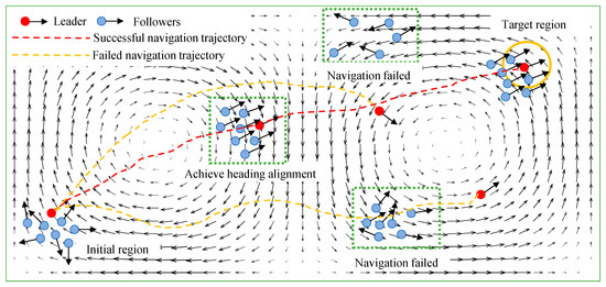
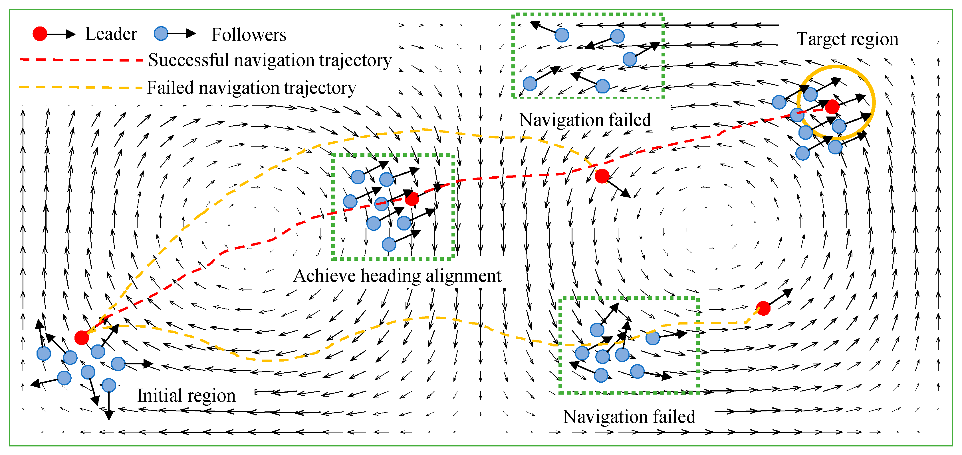
We consider the cooperative navigation of multiple AUVs in a rectangular two-dimensional region influenced by an unsteady double-gyre flow. A behavior-based swarm control model is proposed to accomplish the task. The system consists of N AUVs structured as a hierarchical leader–follower architecture. The leader knows the desired heading and issues navigation commands, while the followers receive these commands directly or indirectly through local interactions. As illustrated in Figure 1, the agents marked in red indicate the leaders, whereas those in blue represent the followers. A trial is deemed successful if the leader guides the group to the target region within a prescribed number of simulation steps. Otherwise, the task is judged to have failed if the group does not reach the target within the time limit, or if loss of connectivity in the communication network breaks the leader- follower topology and causes group fragmentation. Thus, the multi-AUV cooperative navigation task aims to achieve, under flow-field disturbances and under the constraint that only the leader has access to the desired heading, a self-organized transition of the group from an initially disordered state to a stable formation, ensuring that the leader arrives at the target region within the allotted time while maintaining inter-vehicle cohesion and network connectivity.

Figure 1. Schematic of the multi-AUV cooperative navigation task.

3.2. Kinematic and Communication Topology

To investigate the cooperative navigation problem of multi-AUV systems under constant-depth conditions, each autonomous underwater vehicle is abstracted as a point mass with its geometric size neglected, and its motion is described by a two-dimensional single-integrator model. Each agent interacts within a circular neighborhood of radius $R$. Under these approximations, a multi-robot system comprising $N$ AUVs is considered. The communication topology is represented as a directed, weighted graph $G=\left(V,E,{\alpha }_{ij}\left(t\right)\right)$. In this representation, $V=\left\{\mathrm{1,2},\cdots ,N\right\}$ is the set of vertices corresponding to robots, and $E=\left\{\left(i,j\right)\left|i,j\in V,i\ne j\right.\right\}$ represents the directed edges that define communication links. The attention weight ${\alpha }_{ij}\left(t\right)$ describes the value robot i assigns to robot $j$ at a specific time $t$. The corresponding kinematic equation is formulated as:

$${\dot{\mathit{p}}}_i\left(t\right)={\mathit{v}}_i\left(t\right)$$

(1)

where robot $i$’s velocity and position are given by ${\mathit{v}}_i\left(t\right)={\left({\mathit{v}}_{i,x}\left(t\right),{\mathit{v}}_{i,y}\left(t\right)\right)}^{\mathrm{T}}\in {\mathbb{R}}^2$ and ${\mathit{p}}_i\left(t\right)={\left({\mathit{p}}_{i,x}\left(t\right),{\mathit{p}}_{i,y}\left(t\right)\right)}^T\in {\mathbb{R}}^2$, respectively. To ensure safe operation, the speed is bounded by $v^{max}$. When the desired speed exceeds $v^{max}$, the speed will be saturated as:

$${\mathit{v}}_i\left(t\right)={\displaystyle \frac{{\mathit{v}}_i^d\left(t\right)}{‖{\mathit{v}}_i^d\left(t\right)‖}}·min\left\{‖{\mathit{v}}_i^d\left(t\right)‖,v^{max}\right\}$$

(2)

where ${\mathit{v}}_i^d\left(t\right)$ is the desired speed, which will be detailed in Section 4.3. The set of agents neighboring robot$i$ is given by

$${\mathcal{N}}_i\left(t\right)=\left\{j\left|\sqrt{{\left(p_{i,x}\left(t\right)-p_{j,x}\left(t\right)\right)}^2+{\left(p_{i,y}\left(t\right)-p_{j,y}\left(t\right)\right)}^2}\right.<R\right\}$$

(3)

3.3. Metrics

The evaluation framework for collective navigation in a double-gyre flow field is developed from three aspects: task accomplishment, collective motion characteristics, and communication cost. Specifically, the average arrival time is adopted to quantify task execution speed, while the success rate characterizes task completion reliability. The polarization, mean inter-agent distance, and their steady-state values are used to characterize the consistency, cohesion, and stability of the swarm during navigation. In addition, the cumulative communication overhead in a single mission is introduced to quantify the communication cost required to maintain cooperative behavior. Collectively, these metrics provide a comprehensive evaluation of system performance in terms of task outcome, motion process, and communication cost. The specific definitions of these performance metrics are given as follows:

Polarization $\left(\Phi \right)$: measures the consistency of the heading angles of the vehicles and is defined by:

$$\Phi ={\displaystyle \frac{\left|{\sum }_{i=1}^n{\mathit{v}}_i\right|}{\left|{\sum }_{i=1}^n\left|{\mathit{v}}_i\right|\right|}}$$

(4)

where ${\mathit{v}}_{\mathit{i}}$ denotes the speed vector of AUV $i$. When all headings are perfectly aligned, $\Phi =1$. When headings are dispersed, $\Phi$ is close to $0$.

Mean arrival time $\left(\overline{T}\right)$: Over $N_{MC}$ Monte-Carlo simulations, $\overline{T}$ is the average time required for the swarm to travel from the initial region to the target region.

Success rate $\left(P_{suc}\right)$: Subject to a prescribed maximum number of simulation steps, this is the percentage of Monte-Carlo trials in which the swarm reaches the target point. It is computed as:

$$P_{suc}={\displaystyle \frac{M}{N_{MC}}}\times 100\%$$

(5)

where $M$ and $N_{MC}$ denote the number of successful trials and Monte Carlo runs, respectively.

Mean inter-individual distance $\left(\overline{D}\right)$: characterizes swarm cohesion and should remain smooth during ideal motion without sudden fragmentation or compressive deformation [36]. It is defined as:

$$\overline{D}\left(t\right)={\displaystyle \frac{2{\sum }_{i=1}^{N-1}{\sum }_{j=1}^N‖{\mathit{p}}_i\left(t\right)-{\mathit{p}}_j\left(t\right)‖}{N\left(N-1\right)}}$$

(6)

Steady-state value $\left(\delta \right)$: evaluates long-term heading alignment of the swarm. Let $\Phi \left(k\right)$ denote the polarization at time step $k$, and let $T$ be the earliest time step such that $\Phi \left(T\right)>0.95$. The steady-state value $\delta$ is defined by

$$\delta ={\displaystyle \frac{{\sum }_{k=T}^{T+200}\Phi \left(k\right)}{200}}$$

(7)

Cumulative number of communications ($M_{tot}$): This metric is introduced to evaluate the unicast-equivalent cumulative communication cost during a single task execution. Under the assumption that each robot sends one state message to all of its neighbors at each time step, the cumulative number of message transmissions during one task is defined as:

$$M_{tot}=\sum _{t=1}^{T_{arr}}\sum _{i=1}^N{n}_i\left(t\right)$$

(8)

where $T_{arr}$ denotes the arrival horizon of the robot swarm at the target region, expressed in discrete simulation steps, and $n_i\left(t\right)=\left|N_i\left(t\right)\right|$ denotes the number of neighbors of robot i at time t.

4. Behavior-Based Modeling Framework

Building on the preceding multi-AUV cooperative navigation dynamics, a principled behavior-based control architecture is likewise essential. This section presents a behavior-driven swarm control strategy, in which the desired velocity of each agent is formulated as a weighted superposition of three components: alignment, attraction–repulsion, and flow-field disturbance. On this basis, a baseline model is established for operation in a double-gyre flow environment. Meanwhile, a theoretical analysis of the proposed behavioral control law is conducted, providing a rigorous foundation for the subsequent Bayesian optimization of behavioral weights.

4.1. Alignment Term

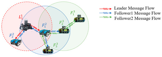
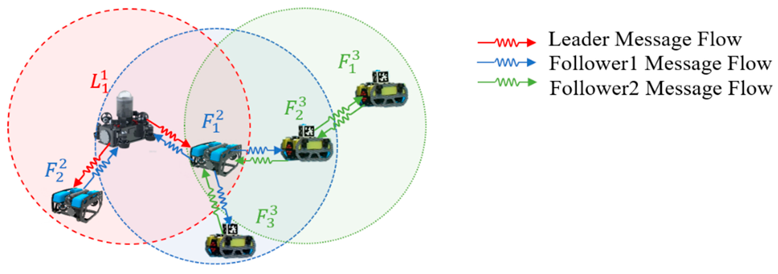
In the DGF-OAS model, the alignment component builds upon the Vicsek model and incorporates a multi-head graph attention mechanism parameterized by the heading angles of the agents [37]. This enables dynamic weighting for individual neighbors, improving the robustness of heading consensus in the presence of disturbances. As illustrated in Figure 2, the swarm adopts a hierarchical leader–follower architecture to amplify the guidance of key nodes. Leaders carry larger weights in the communication topology; therefore, they steer the headings of surrounding robots more effectively.

Figure 2. Interaction topology of a hierarchical leader–follower AUV swarm. Arrows indicate the direction of information flow. The swarm uses a layered leader–follower structure with leaders in the first layer $\left(L_1^1\right)$. The remaining members are dynamically partitioned into the second $\left(F_i^2\right)$ and third $\left(F_i^3\right)$ layers according to their distance from the leader within the communication graph. The dashed circles denote each agent’s interaction range, which limits the effective distance for information exchange.

Let ${\theta }_i\left(t\right)$ represent the heading of the ${AUV}_i$ at discrete time instant $t$. To avoid discontinuities from angular periodicity, we embed headings as ${\mathit{h}}_i\left(t\right)=\left[\cos {\theta }_i\left(t\right),\sin {\theta }_i\left(t\right)\right]$. To mitigate sensor noise and local perturbations, the temporal average for each attention head $h$ is expressed as

$${\overline{\mathit{z}}}_i^{\left(h\right)}\left(t\right)={\displaystyle \frac{1}{\mathrm{∆}}}{\sum }_{k=0}^{\mathrm{∆}-1}{\mathit{h}}_i\left(t-k\right){\mathit{W}}_f^{\left(h\right)}$$

(9)

where $W_f^{\left(h\right)}\in {\mathbb{R}}^{2\times F}$ is the linear projection for head $h$, and $\mathrm{∆}$ is the window length. The unnormalized alignment score on edge $\left(i,j\right)$ is then obtained from:

$${\tilde{e}}_{ij}^{\left(h\right)}\left(t\right)={\left({\mathrm{a}}^{\left(h\right)}\right)}^T\left[{\overline{\mathit{z}}}_i^{\left(h\right)}\left(t\right)‖{\overline{\mathit{z}}}_j^{\left(h\right)}\left(t\right)\right]$$

(10)

where $\parallel$ denotes vector concatenation and ${\mathrm{a}}^{\left(h\right)}$ is the learnable weight vector of head $h$.

To enhance nonlinearity, we apply a LeakyReLU and temperature scaling. Inspired by the stratified social structure observed in pigeon flocks, and in contrast to the role-aware attention in [38], we introduce a role-dependent amplification coefficient ${\gamma }_{ij}$ that scales the contribution of neighbor $j$ in the attention score, defined by:

$$e_{ij}^{\left(h\right)}\left(t\right)={\gamma }_{ij}{\displaystyle \frac{\sigma L\left({\tilde{e}}_{ij}^{\left(h\right)}\left(t\right)\right)}{\tau }},{\gamma }_{ij}=\left\{\begin{array}{c}{\omega }_1 , j=leader\\ {\omega }_2 ,j\in {\mathcal{N}}_{leader}\\ 1 ,otherwise\end{array}\right.$$

(11)

where $\sigma L\left(x\right)=max\left(x,\alpha x\right) \mathrm{w}\mathrm{i}\mathrm{t}\mathrm{h} \alpha \in \left(0,1\right)$ the negative-slope coefficient, and $\tau >0$ is the temperature. ${\mathcal{N}}_{leader}$ denotes the set of neighbors of the leader. The role gains satisfy ${\omega }_1>{\omega }_2>1$, ensuring that, relative to their neighbors, leaders exert stronger influence during information propagation.

Given the scaled scores $e_{ij}^{\left(h\right)}\left(t\right)$, attention weights over the neighbor set ${\mathcal{N}}_i$ of agent $i$ are obtained by a Softmax normalization:

$${\alpha }_{ij}^{\left(h\right)}\left(t\right)={\displaystyle \frac{exp\left(e_{ij}^{\left(h\right)}\left(t\right)\right)}{\sum _{k\in {\mathcal{N}}_i}exp\left(e_{ik}^{\left(h\right)}\left(t\right)\right)}},\forall j\in {\mathcal{N}}_i$$

(12)

With $H$ attention heads in parallel, the final attention weight is defined as the arithmetic mean across heads:

$${\alpha }_{ij}\left(t\right)={\displaystyle \frac{1}{H}}{\sum }_{h=1}^H{\alpha }_{ij}^{\left(h\right)}\left(t\right)$$

(13)

For agent $i$, the alignment component of the desired speed at instant $t$ is expressed as

$${\mathit{v}}_i^{align}\left(t\right)=v_0\left[{\displaystyle \genfrac{}{}{0pt}{}{\mathit{cos}\left({\tilde{\theta }}_i\left(t\right)\right)}{\mathit{sin}\left({\tilde{\theta }}_i\left(t\right)\right)}}\right]$$

(14)

where the consensus heading $\widetilde{{\theta }_i}\left(t\right)$ is computed as the circular mean of the headings of neighboring agents, with weights given by the attention coefficients ${\alpha }_{ij}\left(t\right)$

$${\tilde{\theta }}_i\left(t\right)={\mathit{tan}}^{-1}{\displaystyle \frac{\sum _{j\in N_i\left(t\right)}\left({\alpha }_{ij}\left(t\right)·\mathit{sin}\left({\theta }_j\left(t\right)\right)\right)}{\sum _{j\in N_i\left(t\right)}\left({\alpha }_{ij}\left(t\right)·\mathit{cos}\left({\theta }_j\left(t\right)\right)\right)}}$$

(15)

In (15), ${\alpha }_{ij}\left(t\right)$ are the multi-head attention weights defined above. By jointly accounting for adjacency, communication intensity, and node roles, the proposed alignment mechanism improves collective self-organization and goal consistency of the swarm despite disturbances.

4.2. Attraction and Repulsion Term

Given that heading consensus among robots is secured, maintaining a safe relative spacing through pairwise attraction and repulsion is essential for coherent swarm motion. In this work we adopt the Lennard–Jones potential as the modeling basis for the attraction and repulsion term. Originally proposed by Yamagishi et al. [39] to describe interatomic interactions in molecular dynamics, it is defined as:

$$U\left(d_{ij}\right)=4ϵ\left[{\left({\displaystyle \frac{\sigma }{d_{ij}}}\right)}^{12}-{\left({\displaystyle \frac{\sigma }{d_{ij}}}\right)}^6\right]$$

(16)

where $ϵ$ is the well depth, $\sigma$ represents the characteristic length scale, and $d_{ij}=‖{\mathit{p}}_i-{\mathit{p}}_j‖$ denotes the distance from robot $i$ to its neighboring robot $j$. Physically, the potential induces repulsion when $d_{ij}$ is smaller than the equilibrium separation and attraction when $d_{ij}$ exceeds it (the equilibrium occurs at $d^{*}=2^{1/6}\sigma$). To simplify the analysis, inertia is neglected, and the Lennard–Jones interaction is treated as a direct contribution to the agent’s velocity, derived from the energy-decreasing spatial derivative of the aggregated pairwise interaction function. Accordingly,

$${\mathit{v}}_i^{LJ}\left(t\right)=-\nabla {\sum }_{j\in N_i\left(t\right)}U\left(r_{ij}\right)={\sum }_{j\in N_i\left(t\right)}{\mathit{F}}_{LJ}\left(r_{ij}\right){\mathit{r}}_{ij}$$

(17)

where ${\mathit{r}}_{ij}={\displaystyle \frac{{\mathit{p}}_i-{\mathit{p}}_j}{d_{ij}}}$ denotes the unit direction vector from robot $j$ toward robot $i$, and ${\mathit{F}}_{LJ}\left(r_{ij}\right)$ denotes the magnitude of the interaction force associated with the Lennard–Jones potential. This term prevents collisions while preserving group cohesion, thereby supporting stable swarm operation.

4.3. Flow Field Term

To model ocean disturbances with periodic time variation, we adopt a two-dimensional, time-varying double gyre as the environmental flow field. This flow-field model is widely used for algorithmic validation in geophysical fluid dynamics and underwater robotics. With a small set of parameters, it captures the tidal and seasonal reciprocation and mesoscale vortices that give rise to nonstationarity and spatial inhomogeneity commonly observed in the ocean [40,41]. Therefore, it provides a suitable testbed for multi-AUV cooperative control. Following [42], the stream function can be written as

$$\psi \left(x,y,t\right)=A\mathit{sin}\left(\pi f\left(x,t\right)\right)\mathit{sin}\left(\pi y\right)$$

(18)

$$f\left(x,t\right)={ϵ}_{flow}\mathit{sin}\left(\omega t\right)x^2+\left(1-2{ϵ}_{flow}\mathit{sin}\left(\omega t\right)\right)x$$

(19)

Within a two-dimensional bounded domain, the velocity field follows from the associated stream function as

$$\mathit{v}\left(x,y,t\right)=\left[{\displaystyle \genfrac{}{}{0pt}{}{-\frac{\partial \psi }{\partial y}}{\frac{\partial \psi }{\partial x}}}\right]=\left[{\displaystyle \genfrac{}{}{0pt}{}{-\pi A\mathit{sin}\left(\pi f\left(x,t\right)\right)\mathit{cos}\left(\pi y\right)}{-\pi A\mathit{cos}\left(\pi f\left(x,t\right)\right)\mathit{sin}\left(\pi y\right)\frac{df}{dx}}}\right]$$

(20)

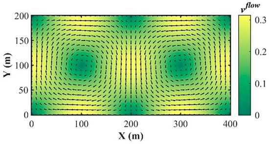
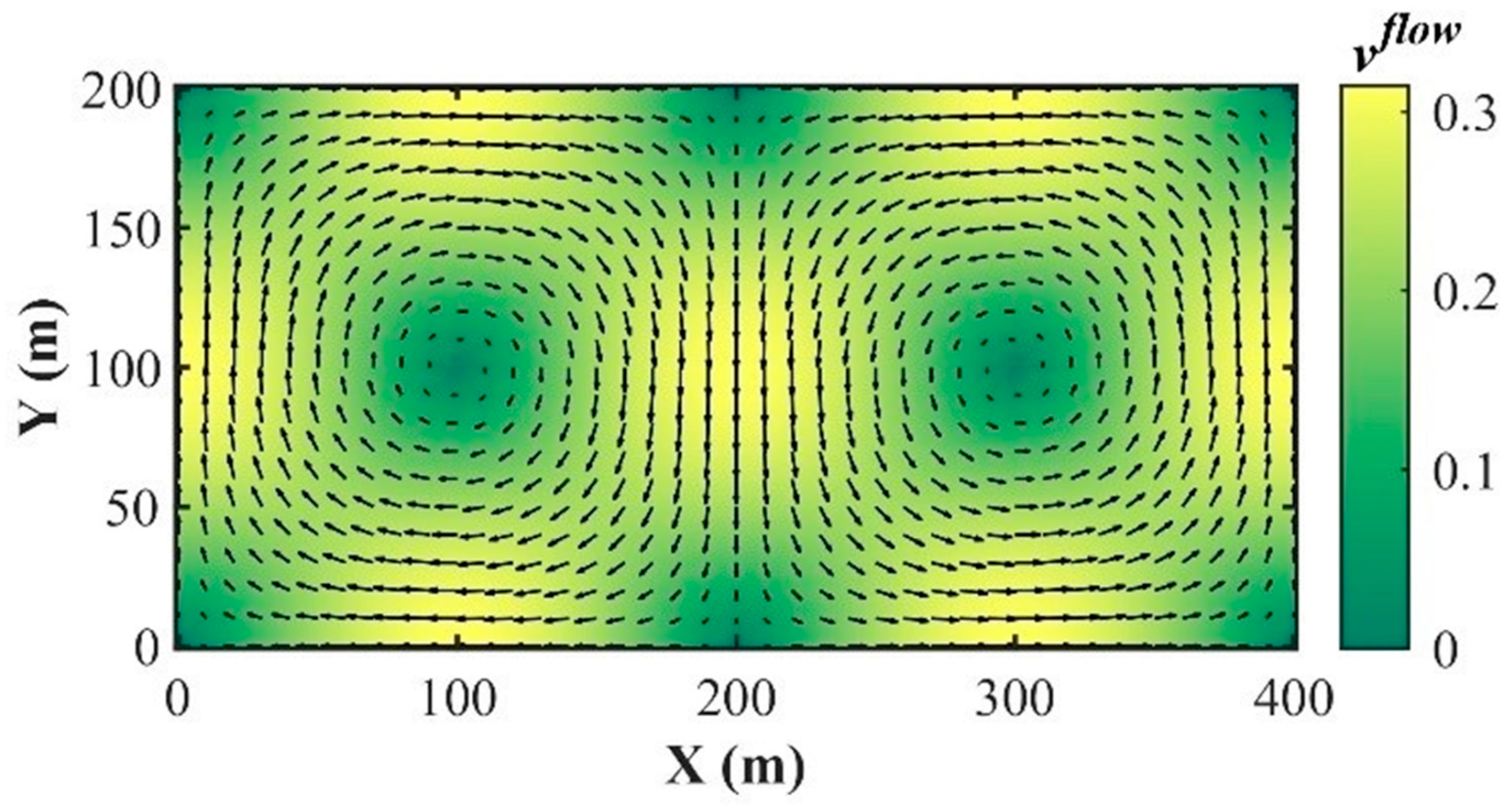
where $A$ is the flow-speed amplitude, $\omega$ is the temporal frequency, and ${ϵ}_{flow}$ controls the time variation in the separatrix between the two gyres. When ${ϵ}_{flow}=0$, the flow consists of two symmetric vortices. When ${ϵ}_{flow}\ne 0$, the separatrix oscillates along the x-axis, causing the two gyres to alternately expand and contract. In this study, the physical space is mapped to the rectangular domain [0,400] × [0,200] (see Figure 3). In addition, each AUV is assumed to access local flow-velocity information at its own position, which is then introduced as an environmental input. In the simulation, this local flow velocity is generated from the double-gyre flow model, with Gaussian noise superimposed to characterize the uncertainty in local sensing. The local flow velocity for AUV i is given by

$${\mathit{v}}_i^{flow}\left(t\right)=\mathit{v}\left(p_i\left(t\right),t\right)+\lambda {\eta }_i\left(t\right)$$

(21)

where $p_i\left(t\right)$ denotes the position of AUV i at time t,${\eta }_i\left(t\right)$ is a Gaussian random perturbation vector, and λ denotes the noise amplitude.

Figure 3. Time-varying double gyre. Arrows indicate the direction and relative magnitude of the velocity field, and the background colormap depicts the speed magnitude (see colorbar at right).

Combining the alignment and the attraction–repulsion terms with the flow contribution, the desired speed of robot $i$ is defined as:

$${\mathit{v}}_i^d\left(t\right)=g^{align}{\mathit{v}}_i^{align}\left(t\right)+g^{lj}{\mathit{v}}_i^{LJ}\left(t\right)+g^{flow}{\mathit{v}}_i^{flow}\left(t\right)$$

(22)

where $g^{align},g^{lj},g^{flow}$ are the corresponding weighting parameters.

The above behavior-level weighted superposition defines a baseline swarm model for AUVs in a double-gyre flow (DGF-AS). In this baseline, all behavior weights used to construct the desired speed are set by manual tuning to serve as a reference for subsequent optimization methods.

4.4. Theoretical Analysis

To investigate the fundamental theoretical properties of the aforementioned multi-AUV cooperative navigation system, the following assumptions are introduced under the conditions that the actual execution velocity satisfies (2) and that the desired velocity of each AUV is generated by the weighted combination of the behavioral terms described above.

Assumption 1.

The initial communication graph G(0) is connected, and the communication topology remains connected throughout the system evolution.

Assumption 2.

The attention weights obtained from (12) and (13) satisfy the nonnegativity and normalization conditions, namely, ${\alpha }_{ij}\left(t\right)\ge 0,\sum _{j\in N_i\left(t\right)}{\alpha }_{ij}\left(t\right)=1$. Moreover, there exists a uniform positive lower bound $\underset{¯}{\alpha }>0$ on every active edge.

Assumption 3.

No collision occurs between any pair of AUVs at the initial time, and the system trajectories remain within a compact collision-free set Ω, the Lennard–Jones potential function is continuously differentiable.

Assumption 4.

The local flow field is bounded over the region of interest. Specifically, there exists a finite positive constant ${\overline{v}}_f$for which $‖\mathit{v}\left({\mathit{p}}_{\mathit{i}}\left(\mathit{t}\right),\mathit{t}\right)‖\le {\overline{\mathit{v}}}_{\mathit{f}}$. Moreover, the random perception disturbance satisfies ${\rm E}\left[{\eta }_i\left(t\right)\right]=0, {\rm E}\left[{‖{\eta }_i\left(t\right)‖}^2\right]\le {\sigma }_{\eta }^2$.

Theorem 1.

Consider the multi-AUV swarm system governed by the dynamic Equation (1), where the actual velocity of each individual is determined by (2), and the desired velocity is composed of the behavioral components in (22), which are respectively defined by (14), (17) and (21). If Assumptions 1–4 hold, then the system possesses the following properties:

1. The group heading error contracts progressively and asymptotically converges to consensus in the absence of external disturbances;

2. The group configuration evolves toward a neighborhood of the potential equilibrium set, and the inter-AUV distances remain bounded;

3. Under flow-field disturbances and random perception errors, the system states remain ultimately bounded.

Appendix A presents the detailed derivation supporting Theorem 1. Furthermore, since the DGF-OAS framework developed in Section 4 only optimizes the behavioral weights in (22) without altering the fundamental structure of the control law, the above conclusions remain valid for the optimized parameterized model as well.

5. DGF-OAS Parameters Optimization

To alleviate the reliance of traditional swarm models on manual tuning guided by experience, particularly in complex underwater environments or large-scale multi-robot tasks, we regard the unknown mapping from behavioral weight parameters to swarm performance as a black box function. Let the weights of the alignment term and the attraction–repulsion term be collected into $\mathit{x}={\left[g^{align},g^{lj}\right]}^T\in \mathsf{\Omega }$. In this study, the flow-field weight $g^{flow}$ is treated as a fixed environmental baseline parameter and therefore is not included in the optimization. Within the prescribed search space $\mathsf{\Omega }$, Bayesian optimization (BO) is used to perform automated, global parameter tuning.

5.1. Objective Function

To jointly optimize multiple performance indicators, the tuning of model weights is formulated as a minimization problem, and the following objective function is introduced:

$$J\left(x\right)={\omega }_s\left(1-\overline{S}\left(\mathit{x}\right)\right)+{\omega }_t\overline{T}\left(\mathit{x}\right)+{\omega }_{\Phi }\left(1-\overline{\Phi }\left(\mathit{x}\right)\right)$$

(23)

where ${\omega }_s$, ${\omega }_t$, and ${\omega }_{\Phi }$ denote the weights associated with the success-probability term, the arrival-time term, and the swarm-consensus term, respectively. To ensure that all performance indicators can be evaluated on a unified scale, the three terms are normalized to the interval [0,1]. Specifically, $\overline{S}\left(\mathit{x}\right)$ denotes the average task success probability over $N_{MC}$ Monte Carlo trials. $\overline{T}\left(\mathit{x}\right)$ denotes the average normalized arrival time over $N_{MC}$ Monte Carlo trials and is defined as $T_{arr}/T_{step}$, where $T_{step}$ is the maximum allowable number of simulation steps. $\overline{\Phi }\left(\mathit{x}\right)$ denotes the average swarm consensus index over the steady-state time window under $N_{MC}$ Monte Carlo trials.

In this work, the weights are set as ${\omega }_s$ = 0.5, ${\omega }_t$ = 0.3, and ${\omega }_{\Phi }$ = 0.2, reflecting a design preference that prioritizes task success while also accounting for execution efficiency and swarm consensus. Therefore, the proposed objective function can comprehensively characterize the consistency, task efficiency, and reliability of the swarm model in complex environments. The optimization process then seeks the optimal parameter pair $\left(g^{align},g^{lj}\right)$ by minimizing $J\left(\mathit{x}\right)$.

5.2. Gaussian Process

Bayesian optimization places a Gaussian process (GP) prior on the objective $J\left(\mathit{x}\right)$. For any finite set $\left\{{\mathit{x}}_1,\cdots ,{\mathit{x}}_{\mathit{n}}\right\}$, the vector of function values $f={\left[J\left({\mathit{x}}_1\right),\cdots ,J\left({\mathit{x}}_{\mathit{n}}\right)\right]}^T$ follows a multivariate normal distribution, that is:

$$J\left(\mathit{x}\right)~\mathcal{G}\mathcal{P}\left[m\left(\mathit{x}\right),k\left(\mathit{x},{\mathit{x}}^{\prime }\right)\right]$$

(24)

We adopt a zero-mean prior, $m\left(\mathit{x}\right)=0$. Since all key swarm-control behavioral parameters to be optimized in this study are continuous variables and the objective function exhibits an overall smooth nonlinear response to parameter variations, the squared exponential (RBF) kernel is employed to model the correlation among sampled points.

$$k\left(\mathit{x},{\mathit{x}}^{\prime }\right)=exp\left(-{\displaystyle \frac{{‖\mathit{x}-{\mathit{x}}^{\prime }‖}^2}{2l^2}}\right)$$

(25)

where $l$ is the length-scale controlling smoothness and correlation range.

5.3. Acquisition Function

The acquisition function quantifies, under the GP posterior, the utility of sampling each candidate $\mathit{x}$, balancing exploration and exploitation [36]. Given that the evaluation of the objective function depends on repeated simulations and thus incurs a relatively high computational cost, the expected improvement (EI) criterion is adopted as the acquisition function in this study.

$$EI\left(\mathit{x}\right)=\left(f\left({\widehat{\mathit{x}}}_{best}\right)-{\mu }_t\left(\mathit{x}\right)-\xi \right)\Psi \left(\widehat{{\rm Z}}\left(\mathit{x}\right)\right)+{\sigma }_t\left(\mathit{x}\right)\varphi \left(\widehat{{\rm Z}}\left(\mathit{x}\right)\right),\widehat{Z}\left(\mathit{x}\right)={\displaystyle \frac{f\left({\widehat{\mathit{x}}}_{best}\right)-{\mu }_t\left(\mathit{x}\right)-\xi }{{\sigma }_t\left(\mathit{x}\right)}}$$

(26)

where ${\mu }_t\left(\mathit{x}\right)$ and ${\sigma }_t\left(\mathit{x}\right)$ denote the posterior mean and standard deviation of the GP model, $f\left({\widehat{\mathit{x}}}_{best}\right)$ represents the highest objective value observed so far, and $\xi >0$ is a parameter controlling exploration. The functions $\Psi \left(·\right)$ and $\varphi \left(·\right)$ denote the standard normal cumulative distribution and its corresponding probability density, respectively. Incorporating evaluation time, the extended EI is computed as:

$${EI}^{+}\left(\mathit{x}\right)={\displaystyle \frac{EI\left(\mathit{x}\right)}{s\left(\mathit{x}\right)+\beta {\sigma }_s\left(\mathit{x}\right)}}$$

(27)

where $s\left(\mathit{x}\right)$ is the predicted evaluation time at $\mathit{x}$, ${\sigma }_s\left(\mathit{x}\right)$ quantifies the uncertainty of that prediction, and $\beta$ is a hyperparameter balancing improvement versus uncertain evaluation cost.

5.4. Parameter Optimization Procedure

Building on the objective in Section 5.1, the Gaussian process surrogate in Section 5.2, and the acquisition function in Section 5.3, the Bayesian optimization procedure for parameter tuning is summarized in Algorithm 1. The procedure comprises four phases: (i) generating $N_0$ initial samples in the search space $\Omega$ and evaluate $J\left(\mathit{x}\right)$ to construct the dataset $\mathcal{D}$; (ii) fitting the Gaussian process surrogate using $\mathcal{D}$; (iii) iteratively sampling candidate points according to the time-aware acquisition ${EI}^{+}$; and (iv) terminating when the maximum number of evaluations is reached or when the improvement over several consecutive iterations falls below a threshold, and select the parameter pair that minimizes $J\left(\mathit{x}\right)$.

Algorithm 1: Bayesian optimization for swarm control weight tuning

$1: \mathcal{D}\leftarrow \mathit{\varnothing }$. $2: \mathrm{Generate} N_0$$\mathrm{initial} \mathrm{samples} \left\{{\mathit{x}}_{\mathit{i}}\right\}\subset \mathsf{\Omega }$. $3: \mathrm{For} \mathrm{each} {\mathit{x}}_{\mathit{i}}$$, \mathrm{evaluate} J\left({\mathit{x}}_{\mathit{i}}\right)$$\mathrm{by} N_{MC}$ simulations; $\mathrm{set} \mathcal{D}\leftarrow \mathcal{D}\cup \left\{\left({\mathit{x}}_{\mathit{i}},J\left({\mathit{x}}_{\mathit{i}}\right)\right)\right\}.$

$4: \mathrm{Fit} \mathrm{a} \mathrm{GP} \mathrm{to} \mathcal{D}$.

$5: \mathbf{for} t=1\dots T_{max}$ do

$6:x_{new}\leftarrow argmax\left\{x\in \mathsf{\Omega }\right\} {EI}^{+}\left(x \left| GP,\mathcal{D}\right.\right)$.

$7:\mathrm{Evaluate} J\left({\mathit{x}}_{\mathit{n}\mathit{e}\mathit{w}}\right)$$\mathrm{by} N_{MC}$ simulations; $\mathcal{D}\leftarrow \mathcal{D}\bigcup \left\{\left({\mathit{x}}_{\mathit{n}\mathit{e}\mathit{w}},J\left({\mathit{x}}_{\mathit{n}\mathit{e}\mathit{w}}\right)\right)\right\}$

$8:\mathrm{Update} \mathrm{the} \mathrm{GP} \mathrm{with} \mathcal{D}$. $9:\mathrm{if} \left|J_{min}^{\left(t\right)}-J_{min}^{\left(t-1\right)}\right|<ϵ$ then break 10: end for $11: {\mathit{x}}^{*}\leftarrow argmin\left\{ J\left({\mathit{x}}_{\mathit{i}}\right):\left({\mathit{x}}_{\mathit{i}},J\left({\mathit{x}}_{\mathit{i}}\right)\right)\in \mathcal{D} \right\}$. $12: \mathbf{return} {\mathit{x}}^{*}$.

The resulting optimal weights $g^{align}$ and $g^{lj}$ are used in the experimental setup of Section 6 for the DGF-OAS model and validated under a temporally varying double-gyre flow. The full DGF-OAS procedure is presented as pseudocode in Algorithm 2.

Algorithm 2: DGF-OAS Model

1: Initialize a DGF field over a $200 \mathrm{m}\times 400 \mathrm{m}$ domain and set the target region. 2: Set flow-field parameters $A,{ϵ}_{flow},\omega ,\lambda$. 3: Use BO to obtain the optimal model weights $g^{align}$ and $g^{lj}$.

4: Randomly initialize the positions and headings of $N$ AUVs; set the initial speed $v_0$.

5: for step = $1,\dots ,T_{step}$ do

6:       for $i=1,\dots ,N$ do

7:           Determine the neighborhood set ${\mathcal{N}}_i$ of ${AUV}_i$.

8:           for $j=1,\dots ,{\mathcal{N}}_i$ do 9:                Calculate $v_i^{align}$ using Equation (14). 10:              Calculate $v_i^{lj}$ using Equation (17). 11:              Calculate $v_i^{flow}$ using Equation (21). 12:         end for 13:         Obtain the AUV speed $v_i$ using Equation (2). 14:         $\mathrm{Update} \mathrm{the} \mathrm{position} \mathrm{of} {AUV}_i$$\mathrm{via} \left[{\displaystyle \genfrac{}{}{0pt}{}{p_{i,x}\left(t+1\right)}{p_{i,y}\left(t+1\right)}}\right]=\left[{\displaystyle \genfrac{}{}{0pt}{}{p_{i,x}\left(t\right)}{p_{i,y}\left(t\right)}}\right]+v_i\mathrm{∆}t\left[{\displaystyle \genfrac{}{}{0pt}{}{\mathit{cos}{\mathit{\theta }}_{\mathit{i}}\left(\mathit{t}\right)}{\mathit{sin}{\mathit{\theta }}_{\mathit{i}}\left(\mathit{t}\right)}}\right]$. 15:     end for 16:     if ${AUV}_i$ reaches the target region, then 17:         Record steps for ${AUV}_i$ to reach the target. 18:         Compute $\Phi \left(step\right)$ using Equation (4). 19:         Compute $\overline{D}\left(\mathrm{s}\mathrm{t}\mathrm{e}\mathrm{p}\right)$ using Equation (6). 20:     end if 21: end for 22: return polarization, average inter-agent distance.

In summary, the proposed method operates in two stages. Stage I employs Bayesian optimization to determine the optimal parameter set, thereby improving model adaptability and robustness under complex flow conditions. Stage II executes behavior control using optimized parameters, enabling efficient and stable swarm motion within a time-varying double-gyre flow field.

6. Simulation Experiments and Results Analysis

The numerical setup and the obtained results are presented and analyzed in this section. First, Bayesian optimization is applied to tune the behavioral weight parameters of the baseline DGF-AS model, resulting in the optimized DGF-OAS model. Then, Monte Carlo simulations are conducted to perform sensitivity analysis on the key model parameters, thereby revealing the effects of different parameter settings on model performance. Moreover, the DGF-OAS model is compared with the DGF-AS model and the leader-based hierarchical perception model in [24], and the differences in collective coordination performance under flow-field environments are quantitatively evaluated using the defined performance metrics. Finally, the contributions of the core components in the DGF-OAS model are investigated through ablation experiments.

6.1. Experimental Setup

Numerical simulations are performed in a periodically varying double-gyre flow field. The swarm comprises a single leader and nineteen followers. The leader AUV is assumed to receive task commands from a base station in real time, and agents form a connected network via local interactions. In each run, all AUVs are initialized at random positions within the prescribed flow-field domain, and their initial headings are drawn uniformly from (0,2π). The main parameters and their values are summarized in Table 1. As shown in Figure 1, the target region is defined as a disk of radius 10 m centered at (370,170). To comprehensively validate the proposed approach, we design four groups of simulations:

Table 1. Model and simulation experimental parameters.

Parameter	Description	Value
N	Number of AUVs	20
R	Sensing radius of AUV	10 m
${ v}_0$	Initial velocity of AUV	0.4 m/s
${ v}_{max}$	Maximum speed of AUV	1 m/s
$\mathrm{∆}t$	Integration step	0.2 s
${ T}_{step}$	Maximum simulation steps	6000
${ N}_{MC}$	Number of MC simulations	60
${ F}_f$	Input feature dimension	2
${ F}_h$	Hidden embedding dimension	4
${ N}_{heads}$	Number of attention heads	4
${ Leaky}_{slope}$	Negative slope in LeakyReLU	0.2
$\tau$	Softmax temperature	1.0
${ \omega }_1,{\omega }_2$	Attention scaling factors	1.5, 1.2
$\sigma$	Characteristic length	7
$ϵ$	Depth of potential function	0.07
A	Flow amplitude	0.068
${ ϵ}_{flow}$	Perturbation strength	0.25
$\omega$	Oscillation rate	$2\mathsf{\pi }$
$\lambda$	Noise amplitude	0.2
${ g}^{flow}$	Flow-field weight	0.72
L	Length of the swarm arena	400 m
W	Width of the swarm arena	200 m

(1) Bayesian Optimization. To identify an appropriate combination of key behavioral weighting parameters in the DGF-OAS model, Bayesian optimization is employed for parameter tuning. The maximum evaluation budget is set to 40, of which the first 8 evaluations are used as initial sampling points to construct the surrogate model. Subsequent samples are then selected adaptively by the acquisition function, thereby achieving a balance between exploration and exploitation in parameter space.

(2) Parameter sensitivity analysis. To elucidate the relationship between DGF-OAS performance and key parameters, we run 60 independent Monte-Carlo trials and analyze the effects of the following variables: flow-speed amplitude (A), oscillation amplitude of the flow-field separatrix (${ϵ}_{flow}$), noise intensity (λ), equilibrium distance (σ),potential-well depth (ϵ), swarm size (N) and attention coefficients $\left({\omega }_1,{\omega }_2\right)$. Their impacts on the polarization and its steady-state level are examined in detail.

(3) Algorithmic performance comparison. For each of the baseline DGF-AS, the proposed DGF-OAS, and the controller of Zhao et al. [24], we run 60 Monte-Carlo trials and evaluate five performance metrics, namely polarization, average inter-agent distance, task success rate, average arrival time, average steady-state level, and cumulative communication count.

(4) Ablation Study. Ablation experiments were designed to examine the contributions of three modules in DGF-OAS: the dynamic attention-weighting mechanism, parameter optimization, and the attraction–repulsion term. Using identical simulation settings, all models were evaluated on a multi-AUV cooperative navigation task in a time-varying double-gyre flow field over 60 Monte Carlo runs. Their cumulative task-success-rate curves were compared to characterize both convergence behavior and final task completion capability.

A practical issue is that different algorithms may require different numbers of steps to reach the target region. Directly comparing raw time-step trajectories can therefore misalign progress and bias the results. To ensure fairness, for each run we linearly map the absolute time axis to a common normalized progress interval [0,1], where 0 denotes the initial state, and 1 denotes the moment of arrival at the target region. We then select equally spaced grid points over [0,1] and obtain metric values at those points via linear interpolation. This procedure guarantees that each algorithm provides data at identical progress points, enabling comparability.

6.2. Bayesian Optimization

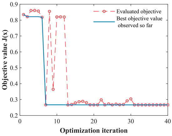
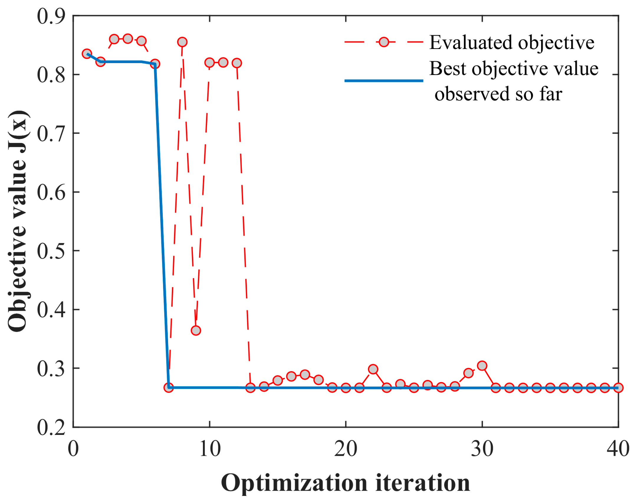
This section analyzes the Bayesian optimization parameter tuning framework for the multi-AUV cooperative navigation task from three perspectives: objective-function convergence, parameter-response characteristics, and sample distribution in the parameter space. As shown in Figure 4, the objective function exhibits a clear convergence trend as the number of evaluations increases. In the early stage of optimization, the objective values of different sample points fluctuate markedly, indicating that the search process is primarily dominated by global exploration. After approximately 13 evaluations, the variation in the objective function decreases significantly, suggesting that the search gradually concentrates on promising regions of the parameter space. Meanwhile, the best-so-far objective value drops rapidly to approximately 0.267 within the first seven evaluations, and then continues to decline slowly until it finally reaches 0.266. These results demonstrate that the proposed optimization process is capable of quickly identifying potentially high-quality regions with relatively few evaluations, thereby exhibiting good convergence performance.

Figure 4. Convergence curve of the objective function during the Bayesian optimization process.

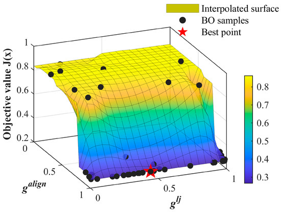
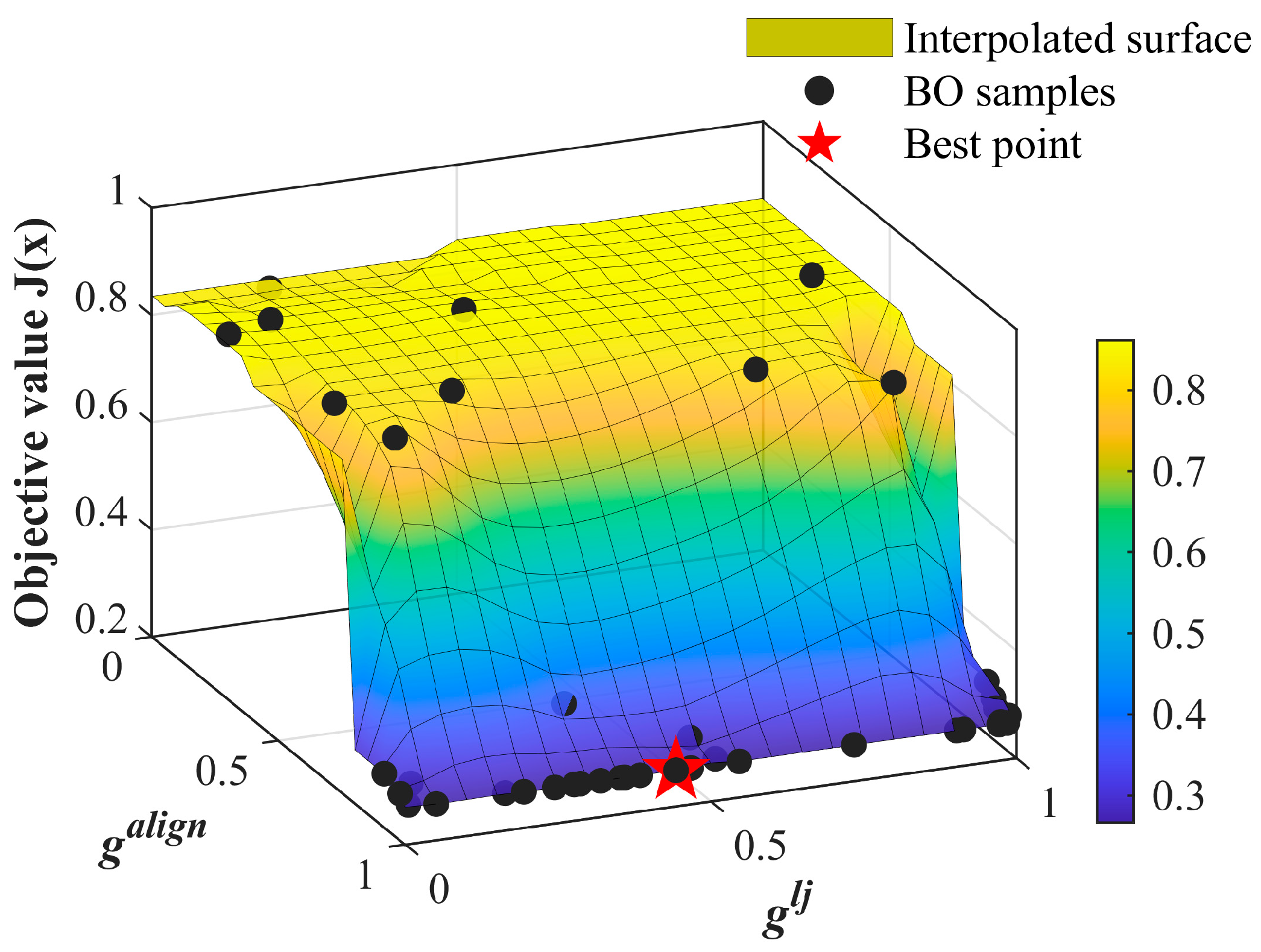
As illustrated in Figure 5, the distribution of the objective function in the behavioral parameter space exhibits a distinctly nonuniform pattern. In the region where $g^{align}$ < 0.51, the objective surface remains relatively flat, indicating that the objective function is only weakly sensitive to variations in $g^{align}$ within this interval. At the same time, the corresponding objective values in this region are generally high, and the sampling points are relatively sparse, suggesting that this area is unlikely to contain promising optima. As $g^{align}$ increases, the surface gradient becomes progressively steeper, indicating that the objective function becomes increasingly sensitive to variations in $g^{align}$. When $g^{align}$ = 0.55 and $g^{lj}$ lies in the range of 0.84–0.99, a pronounced depression appears on the surface, indicating that the objective function becomes relatively sensitive to variations in $g^{lj}$ within this local region. In addition, when $g^{align}$ approaches 0.99, the sampled points become noticeably denser, suggesting that the optimization search progressively concentrates around this advantageous region. Ultimately, the optimal point is obtained at $g^{align}$ = 0.99 and $g^{lj}$ = 0.44, with the minimum objective value reaching 0.266. Considering both the surface morphology and the sampling distribution, it can be observed that $g^{align}$ exerts a stronger overall influence on the objective function than $g^{lj}$. This indicates that, compared with the attraction–repulsion behavioral parameter, the alignment behavioral parameter plays a more significant role in regulating system performance.

Figure 5. Three-dimensional distribution of objective function values in the behavioral parameter space.

6.3. Parameter Sensitivity Analysis

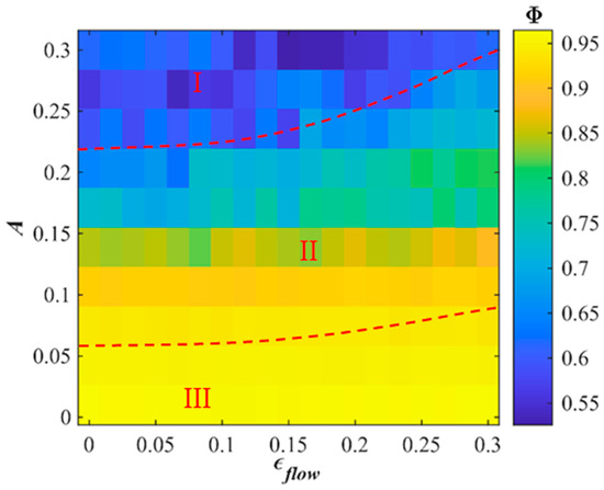
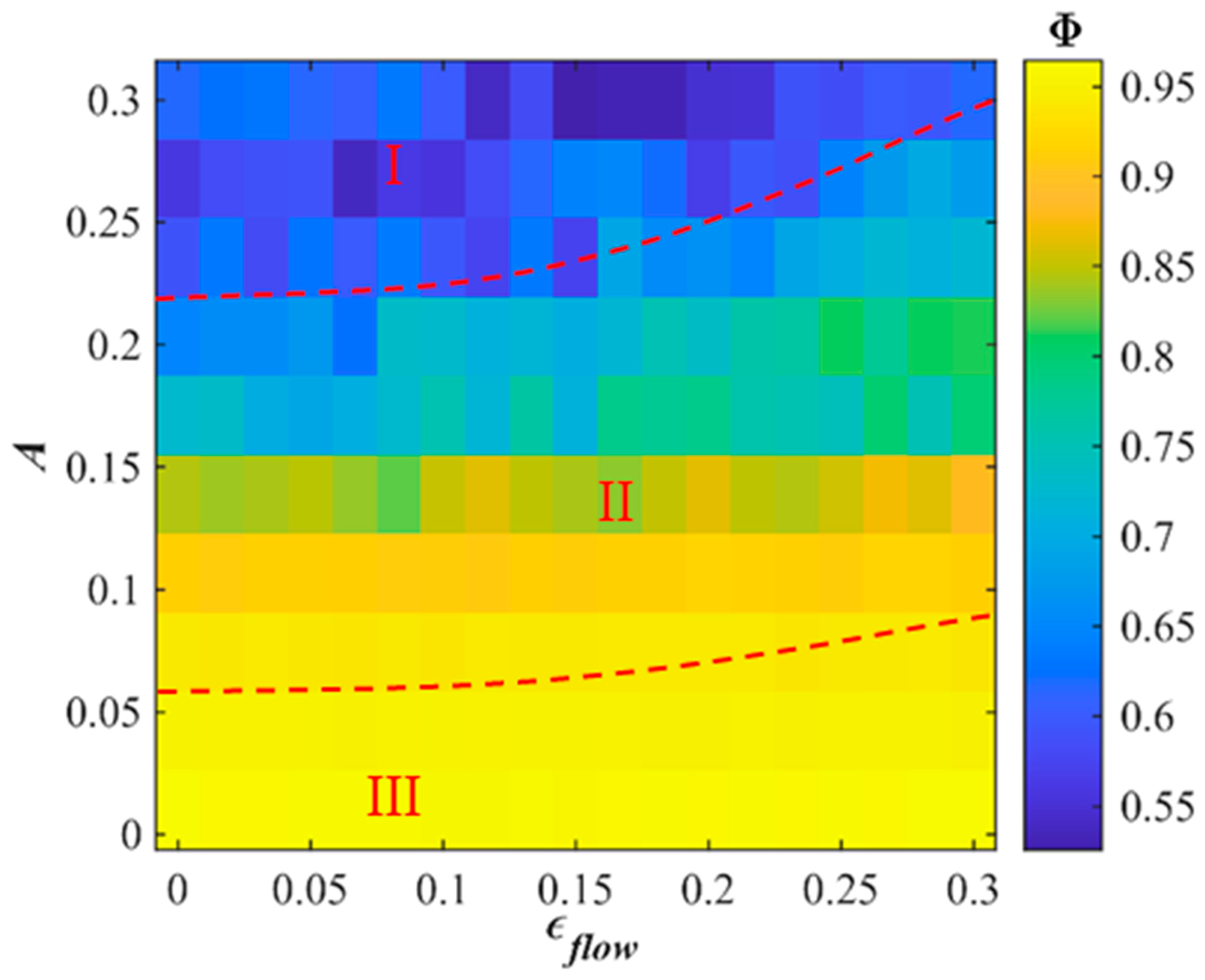
To systematically assess how the flow-speed amplitude $A$ and the oscillation amplitude of the flow-field separatrix ${ϵ}_{flow}$ affect the polarization $\Phi$, we vary only these two parameters while keeping all others fixed. Specifically, we sample $A\in \left[0,0.3\right]$ at 10 uniformly spaced values and ${ϵ}_{flow}\in \left[0,0.3\right]$ at 19 uniformly spaced values, testing every $\left(A,{ϵ}_{flow}\right)$ pair. Figure 6 shows that the $\left(A,{ϵ}_{flow}\right)$ plane can be partitioned into three regimes, I–III, according to $\Phi$. When $A$ increases, the intensified background shear reduces $\Phi$ below 0.63; we designate this interval as the weakly polarized regime (I). As $A$ decreases, $\Phi$ increases; however, increasing ${ϵ}_{flow}$ enlarges the time-varying swing of the separatrix and strengthens vortex perturbations, yielding a transition regime (II) in which the system evolves from weak polarization toward steady behavior. Moderate flow perturbations in regime II can induce heading alignment. When $A<0.058$, $\Phi$ enters the steady regime (III) with $\Phi >0.95$, indicating that DGF-OAS exhibits high adaptability to flow disturbances in this range.

Figure 6. Heatmap of the swarm polarization index $\Phi$ as a function of flow-speed amplitude $A$ and separatrix oscillation amplitude ${ϵ}_{flow}$. Each pixel denotes the mean $\Phi$ over 60 Monte Carlo runs. The parameter space is divided into three states: weak polarization (State I), transition (State II), and stability (State III).

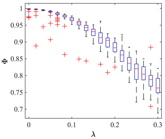
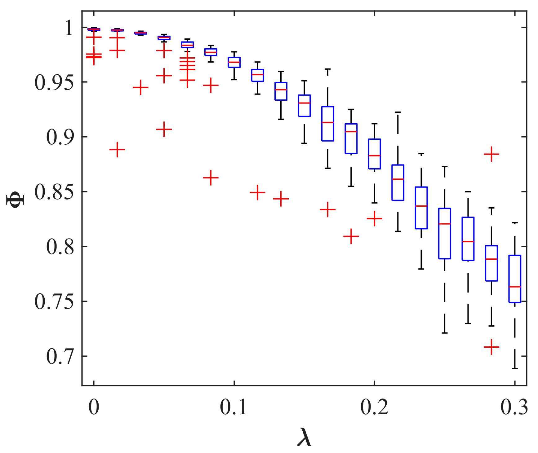
In Equation (21), the noise amplitude λ amplifies flow perturbations and thus influences $\Phi$. To evaluate robustness with respect to λ, we sample λ ∈ [0,0.3] at 19 uniformly spaced values while fixing other parameters. Figure 7 indicates an inverse relationship between $\Phi$ and λ. As λ increases from 0 to approximately 0.12, the polarization level declines but remains in a steady range; for λ further increases from 0.12 to 0.30, $\Phi$ drops to 0.76. This decline is attributable to heightened flow uncertainty that causes frequent neighbor switching and heading fluctuations, thereby weakening alignment. To further quantify the fluctuation characteristics and stability of the results shown in Figure 7, Table 2 presents a statistical summary of group polarization for $\mathsf{\lambda }=0,0.1,0.2,0.3$, covering its average, spread, and 95% confidence range. The results indicate that the mean value of $\Phi$ decreases from approximately 0.997 to 0.766 as the noise intensity increases, while the standard deviation rises from 0.006 to 0.031, suggesting that stronger flow noise leads to more pronounced output fluctuations. At the same time, the 95% confidence intervals remain relatively concentrated for all cases, indicating good statistical stability of the results across repeated simulations. Taken together, Figure 7 and Table 2 show that the DGF-OAS model maintains strong robustness under low-to-moderate noise perturbations, whereas its polarization performance begins to deteriorate noticeably once the noise intensity exceeds a certain range.

Figure 7. Effect of flow-field noise λ on the polarization index $\Phi$ in the DGF-OAS model. Box plots summarize 60 simulation runs; the red line denotes the median, and red plus signs indicate outliers.

Table 2. Group polarization statistics under different flow-noise intensities.

$\mathsf{\lambda }$	Mean	SD	CI
0	0.997	0.006	0.995	0.998
0.1	0.967	0.006	0.966	0.969
0.2	0.882	0.020	0.876	0.887
0.3	0.766	0.031	0.758	0.774

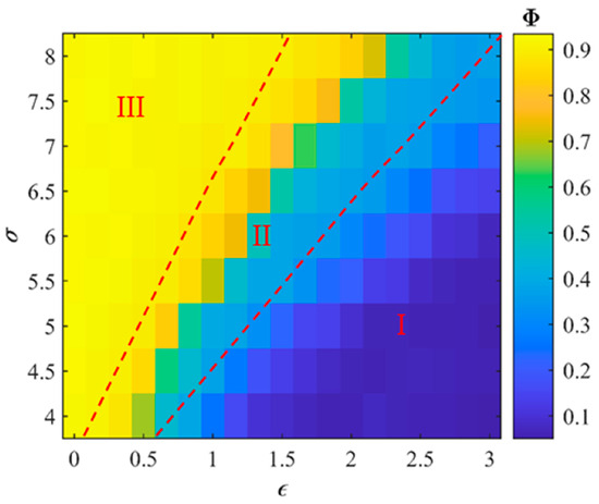
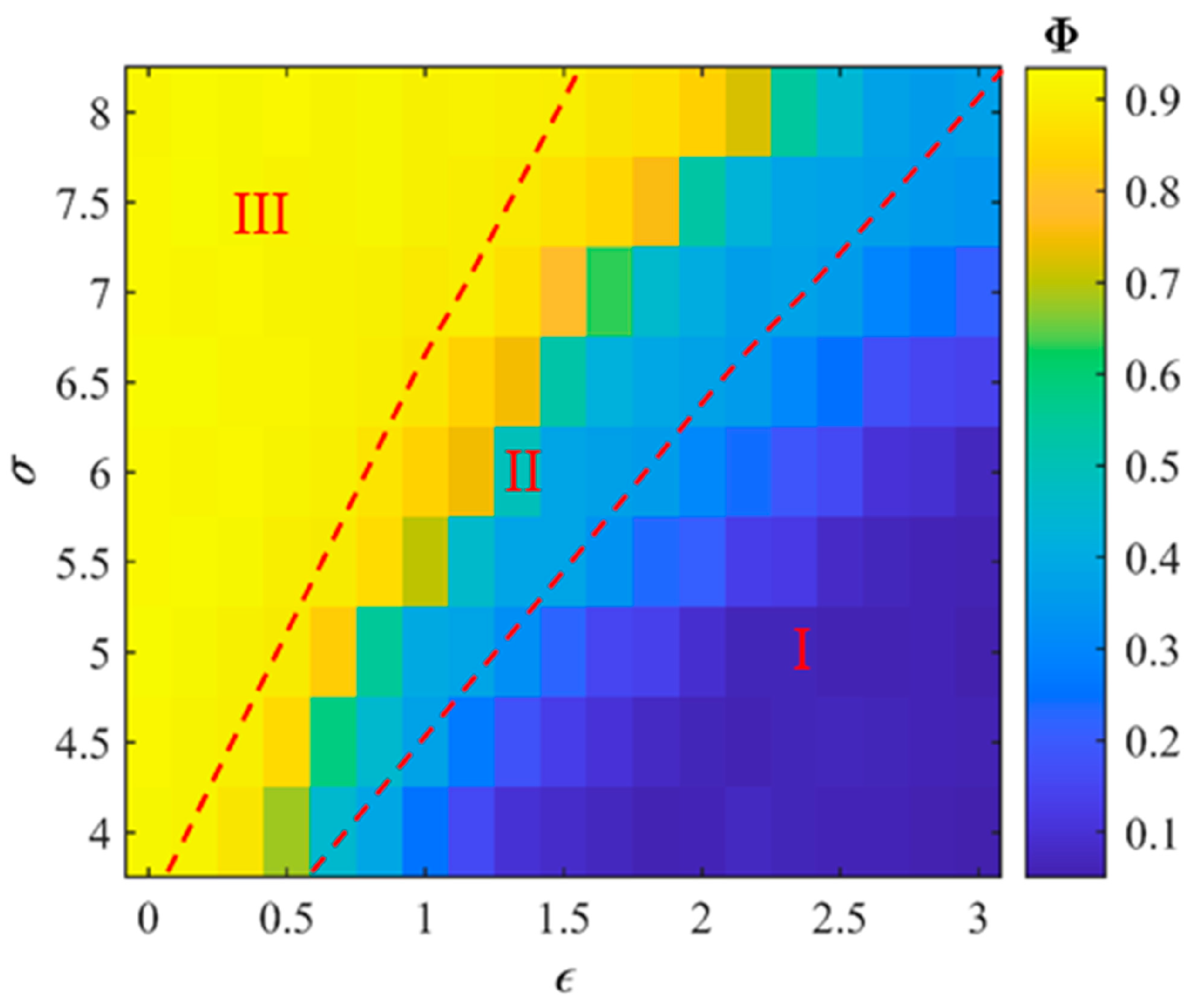
We further examine the sensitivity of $\Phi$ to parameters in the attraction–repulsion term. With all other parameters held fixed, we compute $\Phi$ on a $10\times 19$ Cartesian grid spanning $\sigma \in \left[4,8\right]$ and $ϵ\in \left[0,3\right]$. The results are shown in Figure 8. In regime III, $\Phi$ converges toward $\Phi =0.92$ as $\sigma$ and $ϵ$ increase. In regime II, $\Phi$ lies between 0.40 and 0.90, reflecting a transition from weak polarization to steady behavior. In regime I, the average polarization drops markedly. This is primarily because of the larger potential-well depth $ϵ$ reduces inter-agent spacing, strengthens repulsion, and induces local oscillations, thereby degrading consensus. Hence, when the parameters lie in regime I, DGF-OAS is more sensitive to $\sigma$ and $ϵ$, and swarm performance is more easily affected. Appropriate tuning of the attraction–repulsion parameters is therefore critical for robustness.

Figure 8. Sensitivity of $\Phi$ to $\sigma$ and $ϵ$. Each pixel is the mean over 60 runs. Contours at $\Phi =0.40$ and $\Phi =0.90$ partition the parameter space into three polarization regimes: weak polarization (Regime I), transition (Regime II), and steady state (Regime III).

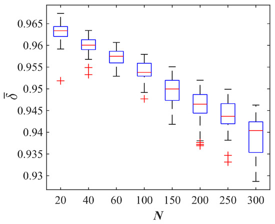
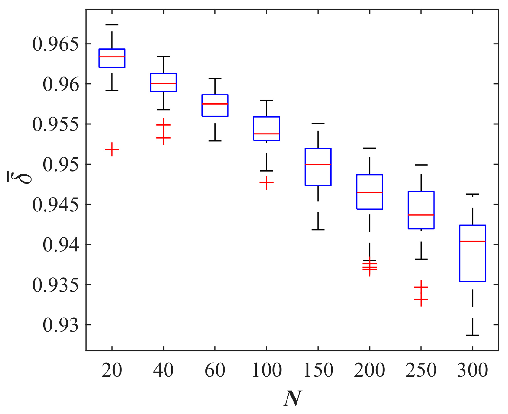
To quantify the influence of swarm size on instability in complex flows, swarms with $N\in \left\{20,40,60,100,150,200,250,300\right\}$, were simulated, and the results are provided in Figure 9. The mean steady-state value $\overline{\delta }$ shows a slight downward trend with increasing $N$, achieving $\overline{\delta }\ge 0.963$ at $N=20$ and $0.940$ by $N=300$. Table 3 presents the mean, standard deviation, and 95% confidence interval of $\overline{\delta }$ under different group sizes. When the number of AUVs is varied between 20 and 300, the mean value of $\overline{\delta }$ declines from 0.963 to 0.939, suggesting a modest reduction in system stability at larger swarm scales. The standard deviation shows only a marginal increase, suggesting that the dispersion of the simulation results becomes slightly larger as the group size grows, while the overall fluctuation level remains low. In addition, the 95% confidence intervals are narrow for all group sizes, implying low uncertainty in the estimation of the mean steady-state value. Overall, the DGF-OAS model exhibits robust steady-state performance under varying group sizes, which supports its scalability for larger swarms.

Figure 9. Box-plot analysis of steady-state values $\overline{\delta }$ versus swarm size $N$. Boxes show the interquartile range. The line within each box represents the median, and the whiskers reach the most distant data points within 1.5 times the interquartile range. Plus signs indicate outliers.

Table 3. Statistical summary of steady-state values under different group sizes.

N	Mean	SD	CI
20	0.963	0.002	0.963	0.964
40	0.960	0.002	0.959	0.960
60	0.957	0.002	0.957	0.958
100	0.954	0.002	0.953	0.955
150	0.949	0.003	0.949	0.950
200	0.946	0.004	0.945	0.947
250	0.944	0.003	0.943	0.944
300	0.939	0.005	0.938	0.940

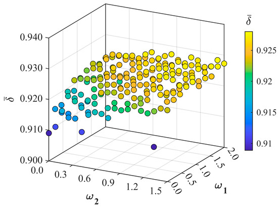
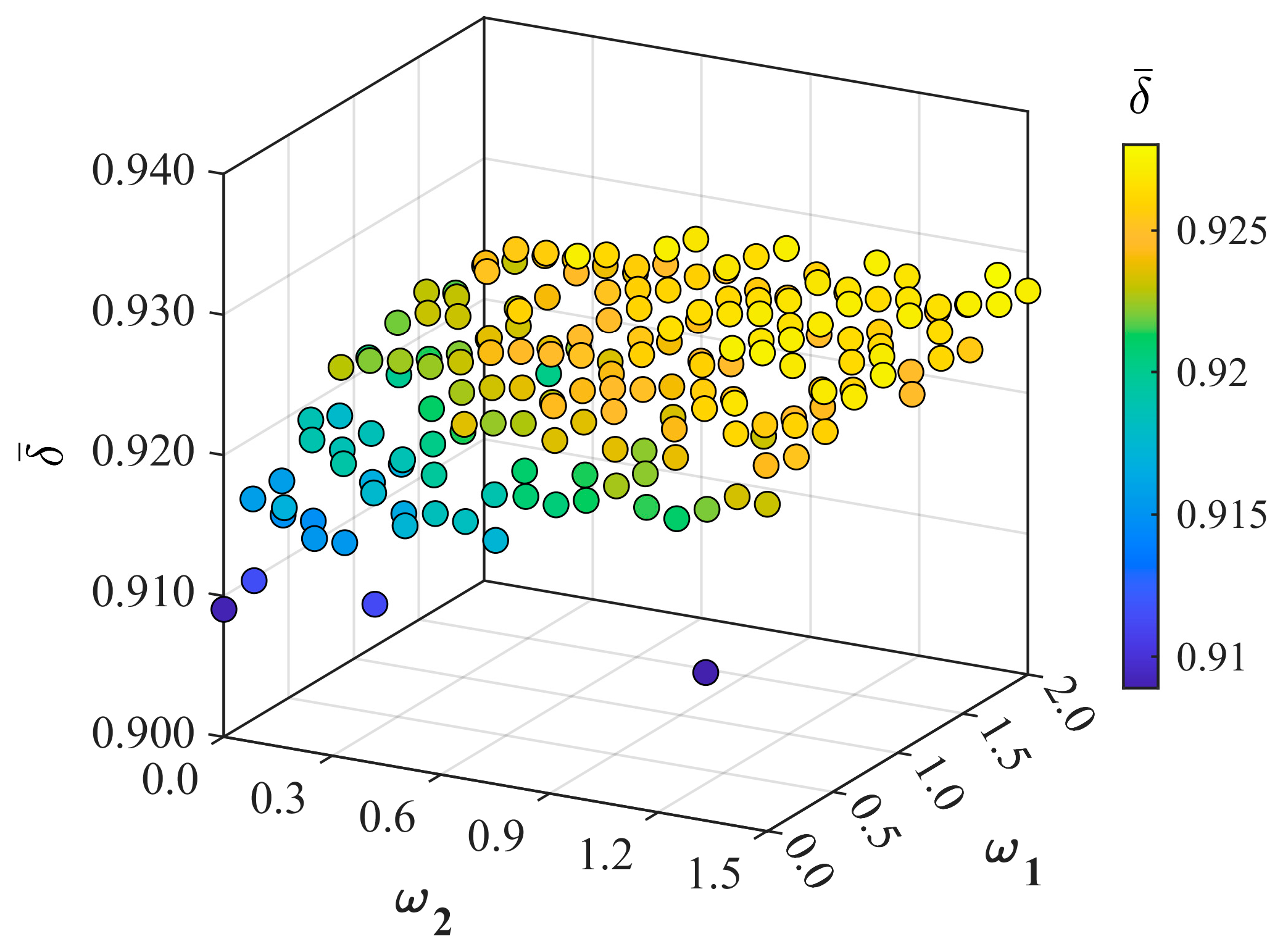
The guidance role of the leader in the leader–follower hierarchical architecture was examined through a parameter sensitivity analysis of the group-averaged steady-state value $\overline{\delta }$ with respect to the role-weight coefficients in Equation (11). Specifically, ${\omega }_1\in \left(\left.0,2\right]\right.$ and ${\omega }_2\in \left(\left.0,1.5\right]\right.$ were sampled using 10 and 19 evenly spaced values, respectively. Figure 10 presents the resulting three-dimensional scatter distribution of $\overline{\delta }$ in the $\left({\omega }_1,{\omega }_2\right)$ parameter space. It can be observed that when ${\omega }_1<0.66$ and ${\omega }_2<1$, the average steady-state value remains below 0.92, indicating that the guiding influence of the leader and its neighboring agents is relatively weak in this region, thereby making it difficult for the swarm to achieve a desirable stable state. As ${\omega }_1$ and ${\omega }_2$ increase, $\overline{\delta }$ exhibits an overall upward trend and stabilizes above 0.925 in the region where ${\omega }_1>1.3$ and ${\omega }_2>1$. This suggests that appropriately increasing the weights assigned to the leader and its neighboring agents can enhance overall swarm stability. Therefore, the parameter region defined by ${\omega }_1>1.3$ and ${\omega }_2>1$ may be regarded as an appropriate choice.

Figure 10. Sensitivity analysis of the role-weight coefficients with respect to the average steady-state value.

In summary, the effects of flow intensity, attraction–repulsion parameters, swarm size, and role-weight coefficients on the overall collective performance were systematically investigated. First, among key flow parameters, both the flow intensity $A$ and the noise amplitude $\lambda$ influence performance; within the tested range, the minimum observed $\Phi$ remains above 0.55, and the separatrix oscillation amplitude ${ϵ}_{flow}$ has a comparatively limited impact. Second, the equilibrium distance $\sigma$ and potential-well depth $ϵ$ in the attraction–repulsion term are more sensitive. In particular, $\Phi$ may drop to $0.1$. Finally, increasing swarm size does not cause substantial performance degradation over the tested range. The role-weight parameters can maintain satisfactory collective performance within an appropriate range of values. Overall, the proposed model exhibits good adaptability under flows of practical intensity and provides guidance for parameter selection in subsequent underwater experiments.

6.4. Performance Comparison of Different Models

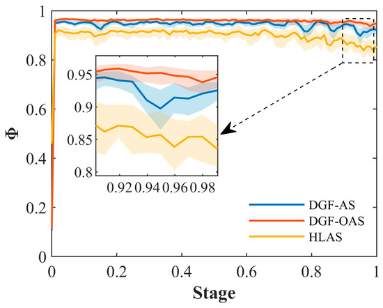
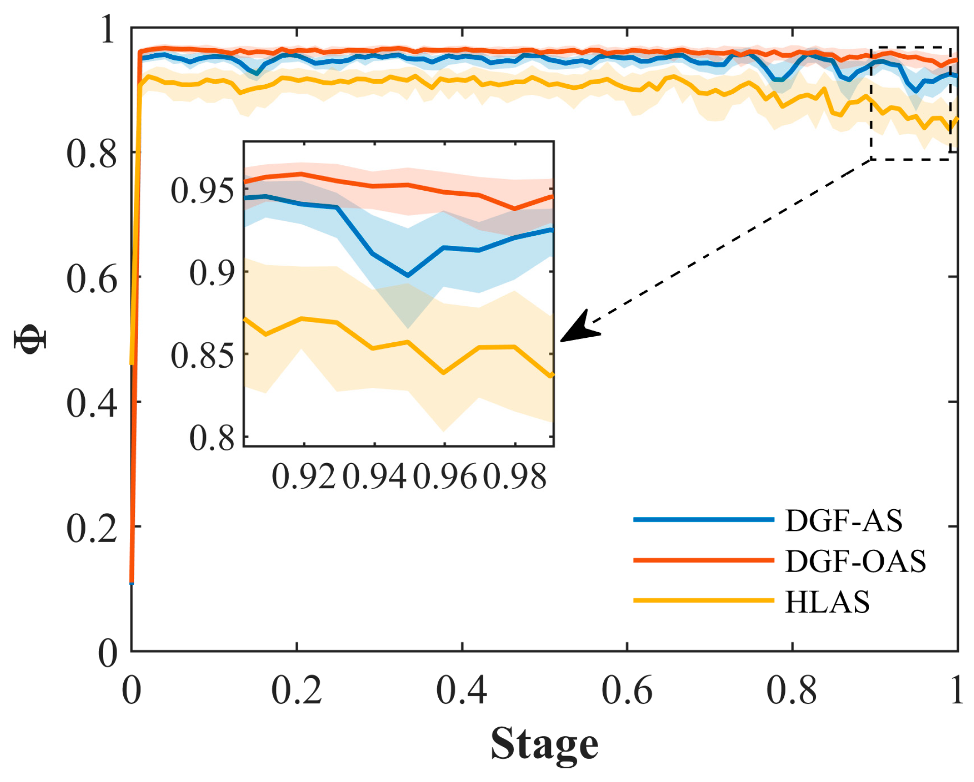
To evaluate the performance of the proposed DGF-OAS model under complex flow conditions, a systematic comparison is conducted against two baseline methods, DGF-AS and HLAS. Figure 11 presents the evolution of swarm polarization as the task progresses across models. In the double-vortex flow, HLAS reaches about 0.92 at the outset but later exhibits pronounced fluctuations due to flow perturbations, with polarization decreasing to 0.84. DGF-AS generally maintains higher polarization than HLAS across stages, but it is more sensitive to flow disturbances and exhibits limited adaptability. By contrast, the Bayesian-optimized DGF-OAS maintains a higher polarization under the same environmental perturbations, indicating superior cooperative performance in complex flow conditions.

Figure 11. Distribution of swarm polarization across task stages. The center solid line represents the median value, whereas the shaded region corresponds to the interquartile interval (Q1−Q3), thus describing data dispersion.

Although polarization effectively captures heading alignment within an AUV swarm, it does not directly quantify whether a coherent spatial structure is preserved.

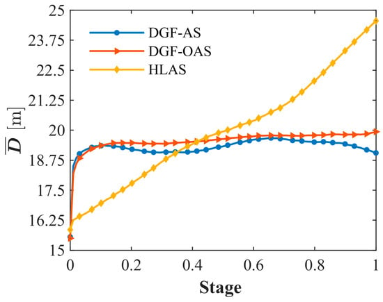
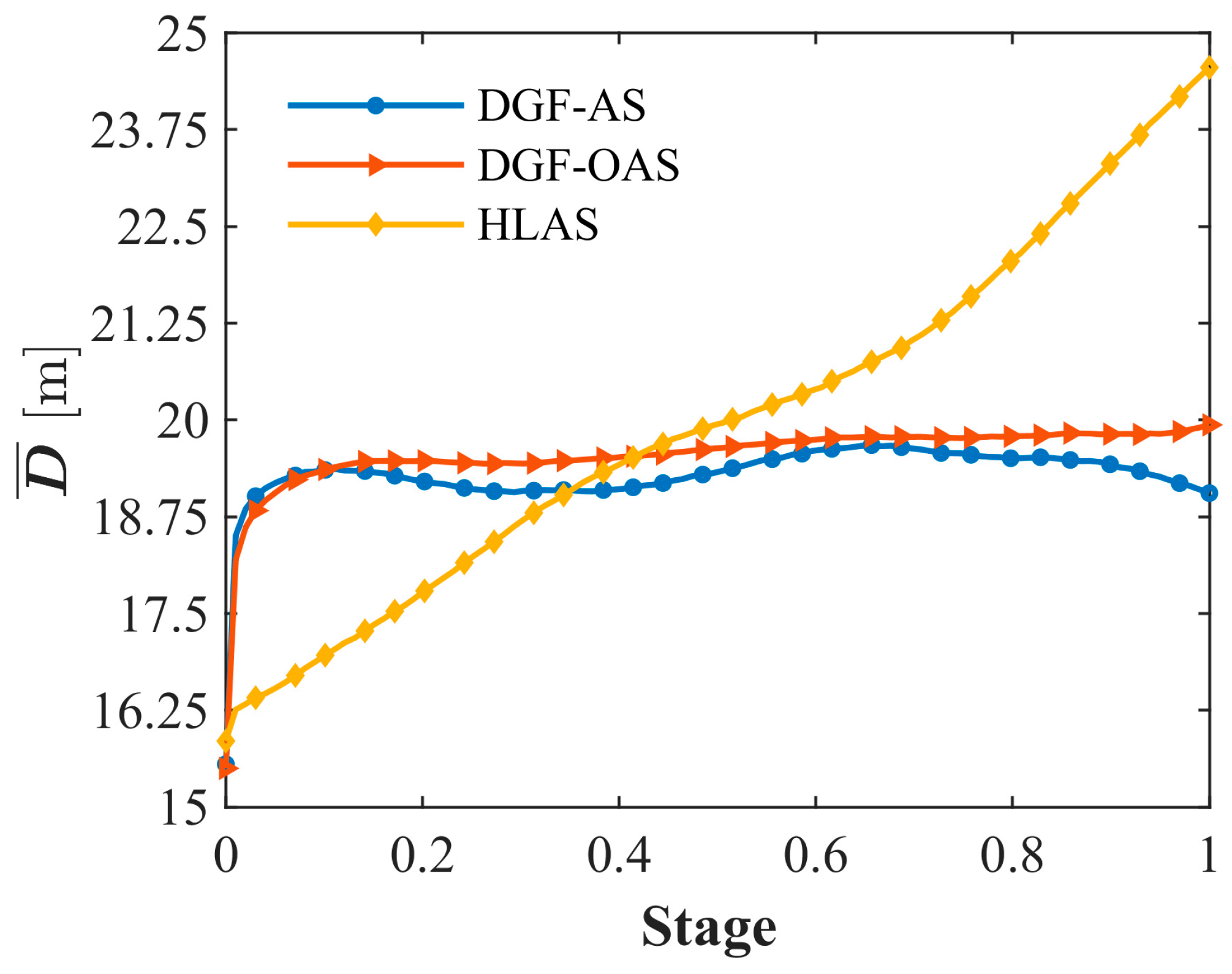
Therefore, cohesion is quantified using the average inter-individual distance $\overline{D}$ given in Equation (6), and the three models are compared in Figure 12. The results show that DGF-OAS drives $\overline{D}$ toward a stable value even under flow perturbations, thereby maintaining high cohesion. In contrast, although the DGF-AS model maintains a relatively small mean inter-agent distance, $\overline{D}$ continues to fluctuate under flow-field disturbances, indicating that its swarm structure is less stable than those of the other models. For HLAS, $\overline{D}$ increases steadily with task progress, which indicates that some AUVs gradually peel away from the formation and separate from the main swarm.

Figure 12. Evolution of the mean inter-individual distance $\overline{D}$ during task execution. Each curve represents the average over $60$ independent simulation runs.

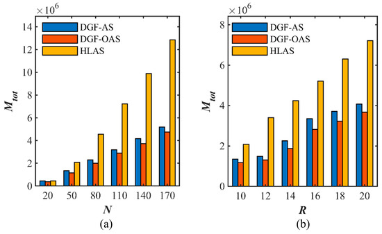
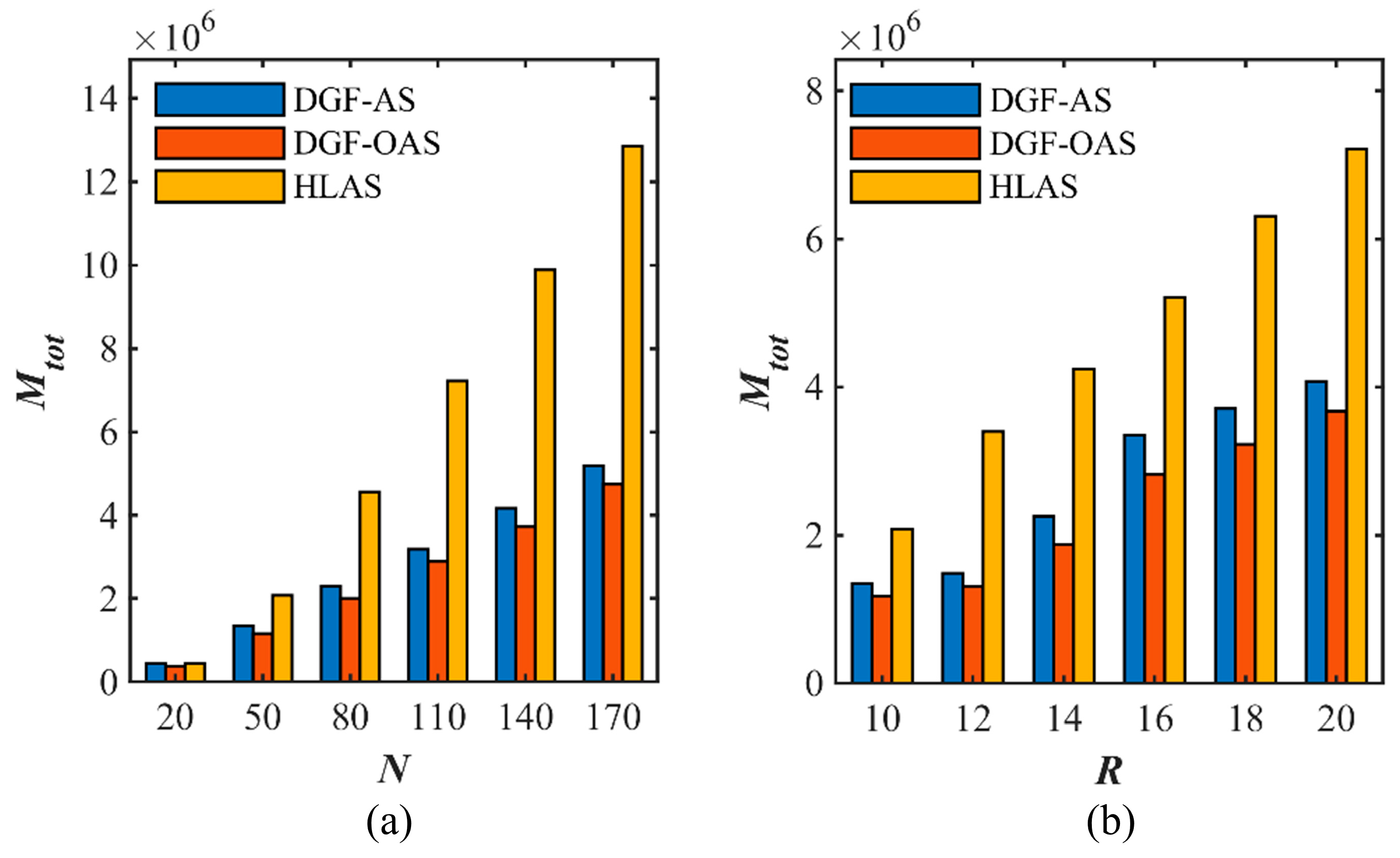
To evaluate the capability of the DGF-OAS model to reduce communication load in flow-field environments, the cumulative communication cost $M_{tot}$, defined in (8), is adopted to compare DGF-OAS with HLAS and DGF-AS under different swarm sizes and interaction radii (see Figure 13a,b). The results show that the cumulative communication cost of all three models increases with the swarm size and interaction radius. This is because larger swarm sizes and larger interaction radii lead to more neighboring agents for each individual, thereby increasing the cumulative communication cost. Nevertheless, compared with HLAS, DGF-OAS consistently achieves lower communication cost under all experimental settings. In particular, when the swarm size is N = 20 and N = 170, the communication cost is reduced by 17.15% and 63.14%, respectively. Under varying interaction radii, DGF-OAS also further reduces the communication cost compared with DGF-AS, with reductions of 12.89% and 9.94% at R = 10 and R = 20, respectively. These results indicate that the DGF-OAS model can effectively reduce the communication load during the swarm cooperation process in flow-field environments.

Figure 13. Comparison of the cumulative communication cost $M_{tot}$ under different parameter settings: (a) $M_{tot}$ for different swarm sizes; (b) $M_{tot}$ for different interaction radii.

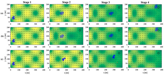
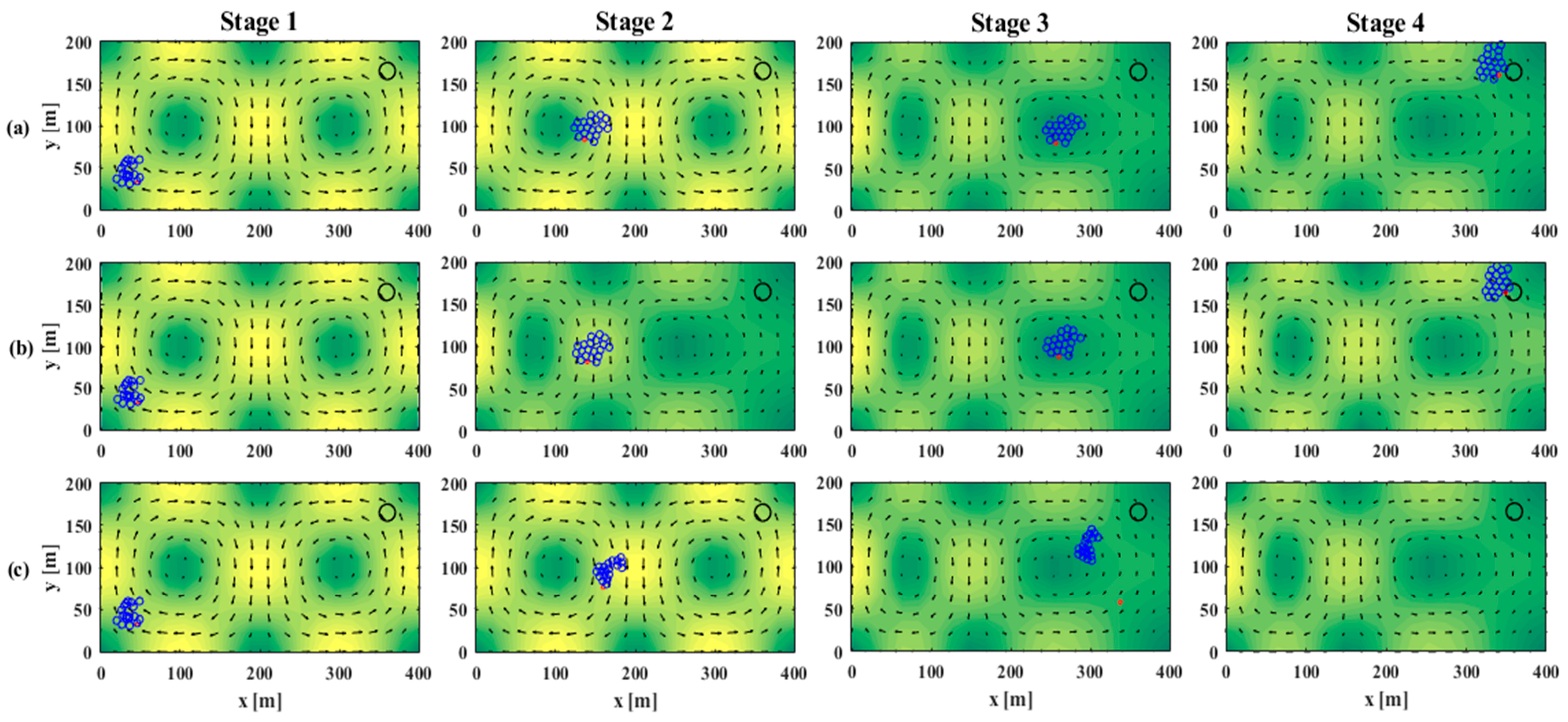
To further assess group behavior across task stages, we randomly sample snapshots from 60 independent simulations and present four representative stages in Figure 14 for a direct comparison of temporal swarm evolution. For DGF-AS and DGF-OAS, Stage 1 begins with randomly dispersed AUVs. After entering the left vortex in Stage 2, the swarm maintains safe inter-vehicle spacing. Within the right vortex in Stage 3, the overall structure remains stable. By Stage 4, although DGF-OAS is affected by the strong flow velocity, rapid local velocity variations, and pronounced shear effects near the target region, it still maintains safe inter-agent spacing and continues to approach the target region. In comparison, DGF-AS fails to reach the target, indicating its inferior task success performance under complex and strongly disturbed flow conditions. HLAS remains disordered at Stage 1. As the simulation advances, the parameterization without explicit treatment of complex flow disturbances yields insufficient neighbor constraints and the swarm progressively fragments. By Stage 4, the swarm has drifted completely out of the flow field. These findings confirm that the proposed model achieves stronger environmental adaptability than the baselines.

Figure 14. Representative snapshots of $N=20$ AUVs across four task stages for three models. (a) DGF-AS. (b) DGF-OAS. (c) HLAS. Columns proceed from Stage 1 to Stage 4 in chronological order.

In the comparative study, we evaluate AUV swarm behavior under flow using three parameterizations, including manually tuned control weights, the optimized weights obtained in Section 5.4, and the control parameters reported in the literature [24]. Unlike Ref. [24], where the attractive and repulsive terms are assigned separate weighting parameters, this paper employs a Lennard–Jones potential to characterize the inter-agent attraction and repulsion in a unified manner. Therefore, $\mathrm{b}\mathrm{o}\mathrm{t}\mathrm{h}{ g}^{rep}$ and $g^{att}$, in this study, correspond to the same weighting parameter $g^{lj}$. Beyond polarization and cohesion, we also assess three metrics defined in Section 3.3, namely task completion rate, mean arrival time, and mean steady-state value. For each parameter set, we perform 60 Monte-Carlo trials and report the mean as the statistic, as summarized in Table 4.

Table 4. Parameter values and performance comparison across algorithms.

Model	${\mathit{g}}^{\mathit{a}\mathit{l}\mathit{i}\mathit{g}\mathit{n}}$	${\mathit{g}}^{\mathit{r}\mathit{e}\mathit{p}}$	${\mathit{g}}^{\mathit{a}\mathit{t}\mathit{t}}$	${\mathit{P}}_{\mathit{s}\mathit{u}\mathit{c}}$(%)	$\overline{\mathit{T}}\left(\mathit{s}\right)$	$\overline{\mathit{\delta }}$
DGF-AS	0.85	0.68	0.68	43	1189.5	0.89
DGF-OAS	0.99	0.44	0.44	97	1001.1	0.93
HLAS [24]	1.00	1.00	0.01	62	1087.2	0.87

Table 4 shows that the proposed DGF-OAS outperforms both baselines across all metrics. The task completion rate reaches 97 percent, which exceeds HLAS at 62 percent and DGF-AS at 43 percent, and demonstrates strong adaptability and robustness in complex flow fields. The mean arrival time for DGF-OAS equals 1001.1 s, markedly faster than the comparison models. The mean steady-state value reaches 0.93, higher than DGF-AS at 0.89 and HLAS at 0.87, which indicates better maintenance of swarm coordination and structural stability during sustained operation. Overall, DGF-OAS delivers higher success rates, faster convergence, and improved steady-state performance, and it provides a clear advantage in challenging hydrodynamic environments.

6.5. Ablation Analysis

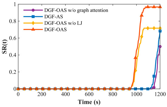
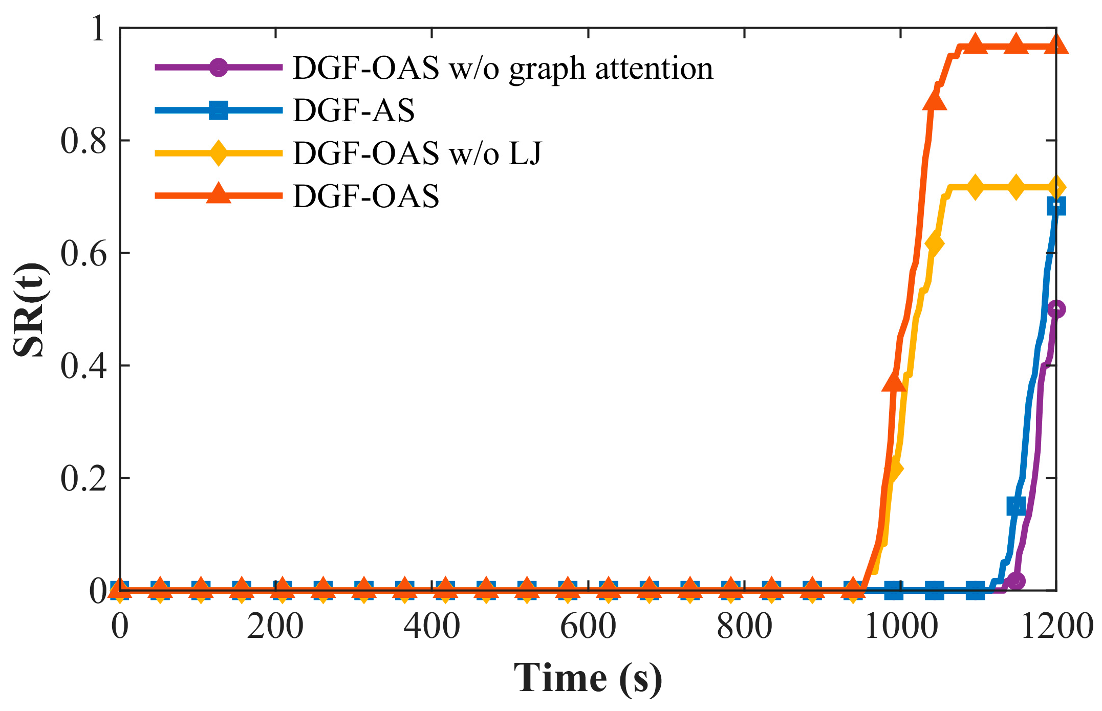
To investigate the effects of the main modules in DGF-OAS, three reduced variants were constructed for comparison, namely, DGF-OAS w/o graph attention, DGF-AS, and DGF-OAS w/o LJ. Figure 15 presents the time evolution of the task success rate, denoted by SR(t), for the different models.

Figure 15. Time evolution of the task success rate, SR(t), for different ablation models.

It is observed that the full DGF-OAS model achieves the earliest increase in SR(t) and attains a final success rate of 0.97 within the maximum simulation horizon, indicating the best overall performance in both task-completion efficiency and mission success. In contrast, removing the Lennard–Jones (LJ) attraction–repulsion term significantly slows the growth of SR(t), and the final success rate drops to 0.72. This degradation suggests that the LJ term plays a critical role in preserving swarm structural coherence and ensuring reliable task completion. The DGF-AS model, in which parameter optimization is omitted, remains consistently below the full model and exhibits an evident rightward shift in the success-rate curve, with a final success rate of 0.68. This result indicates that Bayesian optimization effectively improves the adaptability and execution capability of the model under complex time-varying flow conditions. When the dynamic weight-allocation mechanism is removed, SR(t) grows the slowest and converges to the lowest plateau value of 0.50, demonstrating that this mechanism is particularly important for enhancing cooperative efficiency and improving the overall probability of mission success.

Taken together, the ablation results verify that the graph attention mechanism, Bayesian optimization, and the Lennard–Jones attraction–repulsion term each contribute positively to the cooperative navigation performance of the proposed DGF-OAS model.

7. Conclusions

This study proposes a multi-AUV swarm control model in a Double-Gyre flow environment to improve swarm adaptability and coordination under complex ocean disturbances. By incorporating background flow information, a heading-aware graph attention mechanism, and a Lennard–Jones-potential-based spacing regulation strategy, the proposed model enables the swarm to maintain coordinated motion and stable spatial organization during cooperative navigation. In addition, Bayesian optimization is employed to systematically tune the key behavioral weights, further enhancing the overall cooperative performance of the multi-AUV system. Experiments indicate strong environmental adaptability and robustness within the tested ranges. For flow-intensity amplitudes below 0.058, the DGF-OAS model remains in a steady regime. With flow-field noise amplitudes up to about 40% of the maximum imposed perturbation, the swarm maintains strong heading consensus and is robust to mild to moderate stochastic disturbances. As the attraction–repulsion parameters move from the weak polarization regime to the steady-state regime, swarm polarization increases by 0.50. As swarm size increases from 20 to 300, the mean steady-state value varies by less than 2.39%. Relative to HLAS, the task-completion rate improves by approximately 56.45%, confirming efficient swarm motion under complex hydrodynamic conditions.

Although the proposed model incorporates background flow-field information, it remains limited by the current scenario assumptions and does not explicitly capture the inertia, thruster constraints, and hydrodynamic effects of real AUVs. Future work will focus on incorporating more realistic AUV dynamic models for higher-fidelity simulation studies, as well as conducting physical experiments in real environments to further validate the proposed approach. Such efforts will facilitate the extension of this work to more complex and practical application scenarios.

References

- Masmitja, I.; Palomeras, N.; Toma, D.M.; Bahamon, N.; Carandell, M.; García Del Arco, J.A.; Chatzievangelou, D.; Real, M.; Sánchez-Márquez, A.; Batet, G.; et al. Interconnected Robotic Platforms Inform Deep-Sea Ecological Restoration Trends. Mar. Pollut. Bull. 2025, 219, 118314. [Google Scholar] [CrossRef] [Scilit]
- MahmoudZadeh, S.; Yazdani, A. Distributed Task Allocation and Mission Planning of AUVs for Persistent Underwater Ecological Monitoring and Preservation. Ocean Eng. 2023, 290, 116216. [Google Scholar] [CrossRef] [Scilit]
- Hasan, W.K.; Ahmad, I.; Phung, Q.V.; Habibi, D. Adaptive Guard Band and Power Control for Resource Allocation in Mobile and Fixed Mission-Critical IoUT Networks. Ad Hoc Netw. 2025, 178, 103978. [Google Scholar] [CrossRef] [Scilit]
- Badri-Hoeher, S.; Wilts, T.; Schaefer, L.; Westphalen, J.; Winkler, J.; Isokeit, C.; Harlakin, A.; Hott, M.; Placzek, J.M.; Marx, S.; et al. Multiheterogeneous AUV Swarm Technology Exemplified by the MAUS Project: Cooperation, Mission Planning and Hybrid Communication. IEEE J. Ocean Eng. 2025, 50, 228–251. [Google Scholar] [CrossRef] [Scilit]
- Cai, W.; Ju, Y.; Liu, Z.; Zhang, M.; Lv, S. Event-Triggered Leader-Follower Communication Based Formation Control with Dual-Predictor for Multiple AUVs. Ocean Eng. 2025, 334, 121552. [Google Scholar] [CrossRef] [Scilit]
- Ding, W.; Zhang, L.; Zhang, G.; Wang, C.; Chai, Y.; Yang, T.; Mao, Z. Research on Obstacle Avoidance of Multi-AUV Cluster Formation Based on Virtual Structure and Artificial Potential Field Method★. Comput. Electr. Eng. 2024, 117, 109250. [Google Scholar] [CrossRef] [Scilit]
- Berlinger, F.; Gauci, M.; Nagpal, R. Implicit Coordination for 3D Underwater Collective Behaviors in a Fish-Inspired Robot Swarm. Sci. Robot. 2021, 6, eabd8668. [Google Scholar] [CrossRef] [Scilit]
- Wang, S.; Lin, C.; Han, G.; Zhu, S.; Li, Z.; Wang, Z.; Ma, Y. Multi-AUV Cooperative Underwater Multi-Target Tracking Based on Dynamic-Switching-Enabled Multi-Agent Reinforcement Learning. IEEE Trans. Mob. Comput. 2025, 24, 4296–4311. [Google Scholar] [CrossRef] [Scilit]
- Zhang, Z.; Song, D.; Cao, J.; Zhang, H.; Wang, C.; Xu, H. Multi-Agent Reinforcement Learning for UUV Swarm-Based Capture with Opponent Modeling. In Proceedings of the OCEANS 2025 Brest; IEEE: Brest, France, 2025; pp. 1–7. [Google Scholar]
- Vicsek, T.; Czirok, A.; Ben-Jacob, E.; Cohen, I.; Sochet, O. Novel Type of Phase Transition in a System of Self-Driven Particles. Phys. Rev. Lett. 1995, 75, 1226–1229. [Google Scholar] [CrossRef] [Scilit]
- Jia, Y.; Vicsek, T. Modelling Hierarchical Flocking. New J. Phys. 2019, 21, 093048. [Google Scholar] [CrossRef] [Scilit]
- Liu, X.-F.; Fang, Y.; Zhan, Z.-H.; Jiang, Y.-L.; Zhang, J. A Cooperative Evolutionary Computation Algorithm for Dynamic Multiobjective Multi-AUV Path Planning. IEEE Trans. Ind. Inf. 2024, 20, 669–680. [Google Scholar] [CrossRef] [Scilit]
- Sun, B.; Lv, Z. Multi-AUV Dynamic Cooperative Path Planning with Hybrid Particle Swarm and Dynamic Window Algorithm in Three-Dimensional Terrain and Ocean Current Environment. Biomimetics 2025, 10, 536. [Google Scholar] [CrossRef] [Scilit]
- Pang, W.; Zhu, D.; Sun, C. Multi-AUV Formation Reconfiguration Obstacle Avoidance Algorithm Based on Affine Transformation and Improved Artificial Potential Field under Ocean Currents Disturbance. IEEE Trans. Autom. Sci. Eng. 2024, 21, 1469–1487. [Google Scholar] [CrossRef] [Scilit]
- Gunnarson, P.; Mandralis, I.; Novati, G.; Koumoutsakos, P.; Dabiri, J.O. Learning Efficient Navigation in Vortical Flow Fields. Nat. Commun. 2021, 12, 7143. [Google Scholar] [CrossRef] [Scilit]
- Zhang, Y.; Zheng, S.; Xu, C.; Cai, S. Efficient Navigation in Vortical Flows Based on Reinforcement Learning and Flow Field Prediction. Ocean Eng. 2025, 327, 120937. [Google Scholar] [CrossRef] [Scilit]
- Yu, X.; Hsieh, M.A.; Wei, C.; Tanner, H.G. Synchronous Rendezvous for Networks of Marine Robots in Large Scale Ocean Monitoring. Front. Robot. AI 2019, 6, 76. [Google Scholar] [CrossRef] [Scilit]
- Song, Z.; Lipinski, D.; Mohseni, K. Multi-Vehicle Cooperation and Nearly Fuel-Optimal Flock Guidance in Strong Background Flows. Ocean Eng. 2017, 141, 388–404. [Google Scholar] [CrossRef] [Scilit]
- Jia, Y.; Wang, L. Experimental Implementation of Distributed Flocking Algorithm for Multiple Robotic Fish. Control Eng. Pract. 2014, 30, 1–11. [Google Scholar] [CrossRef] [Scilit]
- Liang, H.; Fu, Y.; Gao, J. Bio-Inspired Self-Organized Cooperative Control Consensus for Crowded UUV Swarm Based on Adaptive Dynamic Interaction Topology. Appl. Intell. 2021, 51, 4664–4681. [Google Scholar] [CrossRef] [Scilit]
- Yin, L.; Yan, Z.; Tian, Q.; Li, H.; Xu, J. A Novel Robust Algorithm for Path Planning of Multiple Autonomous Underwater Vehicles in the Environment with Ocean Currents. Ocean Eng. 2024, 312, 119260. [Google Scholar] [CrossRef] [Scilit]
- Sun, B.; Niu, N. Multi-AUVs Cooperative Path Planning in 3D Underwater Terrain and Vortex Environments Based on Improved Multi-Objective Particle Swarm Optimization Algorithm. Ocean Eng. 2024, 311, 118944. [Google Scholar] [CrossRef] [Scilit]
- Mu, X.; Gao, W. Coverage Path Planning for Multi-AUV Considering Ocean Currents and Sonar Performance. Front. Mar. Sci. 2025, 11, 1483122. [Google Scholar] [CrossRef] [Scilit]
- Zhao, Q.; Yang, T.; Tang, G.; Yang, Y.; Luan, Y.; Wang, G.; Wan, T.; Xu, M.; Li, S.; Xie, G. Hierarchical Model for an AUV Swarm with a Leader. Pol. Marit. Res. 2025, 32, 71–80. [Google Scholar] [CrossRef] [Scilit]
- Zhao, Q.; Luan, Y.; Li, S.; Wang, G.; Xu, M.; Wang, C.; Xie, G. The Influences of Self-Introspection and Credit Evaluation on Self-Organized Flocking. Appl. Sci. 2023, 13, 10361. [Google Scholar] [CrossRef] [Scilit]
- Li, J.; Chen, Q.; Wang, Y. A Multi-Auv Adaptive Collaborative Target Coverage Algorithm for Unknown Environment. Ad Hoc Netw. 2026, 180, 104033. [Google Scholar] [CrossRef] [Scilit]
- Zhu, R.; Boukerche, A.; Feng, L.; Yang, Q. A Trust Management-Based Secure Routing Protocol with AUV-Aided Path Repairing for Underwater Acoustic Sensor Networks. Ad Hoc Netw. 2023, 149, 103212. [Google Scholar] [CrossRef] [Scilit]
- Sahu, B.K.; Subudhi, B. Flocking Control of Multiple AUVs Based on Fuzzy Potential Functions. IEEE Trans. Fuzzy Syst. 2018, 26, 2539–2551. [Google Scholar] [CrossRef] [Scilit]
- Tao, H.; Shao, M.; Wang, Y.; Wang, X.; Luo, H. Multi-UAV Assisted Cross-Boundary Communication Scheme for AUV Swarms via Multi-Agent Reinforcement Learning Approach. Ad Hoc Netw. 2025, 178, 103993. [Google Scholar] [CrossRef] [Scilit]
- Nitti, A.; De Tullio, M.D.; Federico, I.; Carbone, G. A Collective Intelligence Model for Swarm Robotics Applications. Nat. Commun. 2025, 16, 6572. [Google Scholar] [CrossRef] [Scilit] [PubMed]
- Zhang, J.; Ning, X.; Ma, S. An Improved Particle Swarm Optimization Based on Age Factor for Multi-AUV Cooperative Planning. Ocean Eng. 2023, 287, 115753. [Google Scholar] [CrossRef] [Scilit]
- Sun, B.; Li, Y.; Zhang, W. Multipopulation Grey Wolf Optimization for Cooperative Multi-AUV Path Planning in Complex Underwater Environments. IEEE Syst. J. 2025, 19, 837–847. [Google Scholar] [CrossRef] [Scilit]
- Ma, L.; Bao, W.; Zhu, X.; Wu, M.; Wang, Y.; Ling, Y.; Zhou, W. O-Flocking: Optimized Flocking Model on Autonomous Navigation for Robotic Swarm. In Advances in Swarm Intelligence; Tan, Y., Shi, Y., Tuba, M., Eds.; Lecture Notes in Computer Science; Springer International Publishing: Cham, Switzerland, 2020; Volume 12145, pp. 628–639. ISBN 978-3-030-53955-9. [Google Scholar]
- Vásárhelyi, G.; Virágh, C.; Somorjai, G.; Nepusz, T.; Eiben, A.E.; Vicsek, T. Optimized Flocking of Autonomous Drones in Confined Environments. Sci. Robot. 2018, 3, eaat3536. [Google Scholar] [CrossRef] [Scilit]
- Bezcioglu, M.B.; Lennox, B.; Arvin, F. Self-Organised Swarm Flocking with Deep Reinforcement Learning. In Proceedings of the 2021 7th International Conference on Automation, Robotics and Applications (ICARA); IEEE: Prague, Czech Republic, 2021; pp. 226–230. [Google Scholar]
- Mezey, D.; Bastien, R.; Zheng, Y.; McKee, N.; Stoll, D.; Hamann, H.; Romanczuk, P. Purely Vision-Based Collective Movement of Robots. npj Robot. 2025, 3, 11. [Google Scholar] [CrossRef] [Scilit]
- Veličković, P.; Cucurull, G.; Casanova, A.; Romero, A.; Liò, P.; Bengio, Y. Graph Attention Networks. arXiv 2017, arXiv:1710.10903. [Google Scholar]
- Huang, Z.; He, Y.; Wang, S.; Wang, Z.; Xu, R.; Merothra, S. SRACas: A Social Role-Aware Graph Neural Network-Based Model for Popularity Prediction of Information Cascades. In Proceedings of the Database Systems for Advanced Applications; Wang, X., Sapino, M.L., Han, W.-S., El Abbadi, A., Dobbie, G., Feng, Z., Shao, Y., Yin, H., Eds.; Springer Nature: Cham, Switzerland, 2023; Volume 13945, pp. 21–30. [Google Scholar]
- Yamagishi, K.; Suzuki, T. Collective Movement Method for Swarm Robot Based on a Thermodynamic Model. Int. J. Adv. Comput. Sci. Appl. 2017, 8, 513–519. [Google Scholar] [CrossRef] [Scilit]
- Michini, M.; Hsieh, M.A.; Forgoston, E.; Schwartz, I.B. Experimental Validation of Robotic Manifold Tracking in Gyre-like Flows. In Proceedings of the 2014 IEEE/RSJ International Conference on Intelligent Robots and Systems; IEEE: Chicago, IL, USA, 2014; pp. 2306–2311. [Google Scholar]
- Mei, J.; Kutz, J.N.; Brunton, S.L. Observability-Based Energy Efficient Path Planning with Background Flow via Deep Reinforcement Learning. In Proceedings of the 2023 62nd IEEE Conference on Decision and Control (CDC); IEEE: Singapore, 2023; pp. 4364–4371. [Google Scholar]
- Shadden, S.C.; Lekien, F.; Marsden, J.E. Definition and Properties of Lagrangian Coherent Structures from Finite-Time Lyapunov Exponents in Two-Dimensional Aperiodic Flows. Phys. D Nonlinear Phenom. 2005, 212, 271–304. [Google Scholar] [CrossRef] [Scilit]
Disclaimer/Publisher’s Note: The statements, opinions and data contained in all publications are solely those of the individual author(s) and contributor(s) and not of MDPI and/or the editor(s). MDPI and/or the editor(s) disclaim responsibility for any injury to people or property resulting from any ideas, methods, instructions or products referred to in the content. |
© 2026 by the authors. Licensee MDPI, Basel, Switzerland. This article is an open access article distributed under the terms and conditions of the Creative Commons Attribution (CC BY) license.