


Highlights
What are the main fundings?
- A hierarchical navigation architecture integrating deep representation learning with an improved Vortex Artificial Potential Field is proposed, achieving O(1) constant-time inference (35.05 ± 2.76 ms) independent of obstacle density, validated across 3–35 obstacles with ANOVA (p = 0.391) and Pearson correlation (r = 0.29). The proposed Vortex APF controller effectively suppresses the Goal Non-Reachable with Obstacles Nearby problem and limit-cycle oscillations through tangential rotational forces and adaptive forward driving force, improving trajectory smoothness by 12.8-fold (mean turning angle reduced from 54.15° to 4.22°).
- A closed-loop replanning mechanism integrates neural network global reasoning with APF local optimization, triggering adaptive replanning based on tracking deviation and motion state to ensure robust performance in dynamic environments. Comprehensive experiments across four difficulty levels demonstrate a 91% success rate in dense environments, with 35% reduction in computation time compared to RRT*, while maintaining superior trajectory quality.
What are the implications of the main findings?
- The O(1) constant-time inference provides predictable and stable computational performance, making the method particularly suitable for resource-constrained UAV platforms operating in GPS-denied or obstacle-rich environments.The Vortex APF offers a unified analytical solution to long-standing APF limitations (GNRON and oscillations), enhancing both safety and flight efficiency for high-speed UAV navigation.
- The hierarchical architecture strikes a favorable balance between global path optimality and real-time local avoidance, enabling robust autonomous navigation in challenging real-world scenarios such as warehouses, forests, and disaster sites. The framework is extensible to multi-UAV coordination and dynamic obstacle handling, providing a foundation for future research in swarm robotics and adaptive control under uncertainty.
Abstract
Existing autonomous navigation systems for Unmanned Aerial Vehicles (UAVs) face the dual challenges of local minima entrapment and computational complexity that scales with environmental density. This paper proposes a hierarchical navigation architecture integrating deep representation learning with an improved Vortex Artificial Potential Field (APF). At the decision layer, a Convolutional Neural Network (CNN) encodes the environment as a fixed-dimensional tensor and generates global waypoints with constant-time inference, independent of obstacle count. At the control layer, a Vortex APF resolves the Goal Non-Reachable with Obstacles Nearby (GNRON) problem and limit-cycle oscillations through tangential rotational potentials, achieving significant improvement in trajectory smoothness compared to traditional APF methods. A closed-loop replanning mechanism further ensures robust performance under execution drift. Experiments across varying obstacle densities demonstrate that the combined system achieves high navigation success rates in dense environments with substantially reduced computation time compared to sampling-based planners such as Rapidly exploring Random Tree star (RRT*), while maintaining superior trajectory quality. This architecture provides a computationally efficient solution for resource-constrained UAV platforms operating in GPS-denied or obstacle-rich environments such as warehouses, forests, and disaster sites.
1. Introduction
The adaptive motion planning mechanisms exhibited by living organisms in complex and dynamic environments have long served as a benchmark for biomimetic research in the field of intelligent robotics [1,2,3,4]. However, existing autonomous systems still commonly suffer from local minima entrapment or trajectory oscillations in unstructured or high-density obstacle scenarios, highlighting their limited adaptability in complex habitats. Fundamentally, this performance gap stems from an essential difference in environmental perception paradigms: biological intelligence leverages multimodal sensing and prior spatiotemporal knowledge to intuitively construct global topological paths, whereas traditional robots are constrained by local observation fields and often rely on incremental trial-and-error exploration to build connectivity graphs, making it difficult to efficiently exploit the global geometric features of the environment [5].
For Unmanned Aerial Vehicles (UAVs), these navigation challenges are further amplified by strict onboard constraints. Unlike ground robots, UAVs operate under stringent payload limitations—typical quadrotors must allocate weight budgets across sensors, batteries, and computing hardware [6]. The limited onboard processors cannot afford computationally intensive iterative sampling methods that scale linearly or exponentially with scene complexity [7]. Additionally, battery-powered flight imposes strict energy constraints: flight endurance of only 15–20 min, leaving limited computational budget for navigation tasks [8]. More critically, UAV navigation demands deterministic planning latency—high-speed flight at 3–5 m/s requires <100 ms planning cycles to avoid collisions, yet traditional sampling-based algorithms (RRT*, PRM) exhibit unpredictable time complexity that fluctuates with obstacle density [9]. These factors collectively necessitate navigation algorithms with constant-time complexity and minimal memory footprint.
These considerations motivate the need for a navigation framework that simultaneously addresses three fundamental challenges: achieving constant-time global planning independent of obstacle density, resolving local minima and oscillation problems in potential field control, and integrating both levels into a robust closed-loop architecture. Inspired by the biological dual-mode navigation mechanism of global intuitive guidance—local fine-tuned control—this paper proposes a hierarchical navigation architecture that deeply integrates deep representation learning with analytical potential field control. At the decision layer, an end-to-end deep feature extractor is employed to directly map high-dimensional environmental tensors to a sequence of waypoints. By encoding features, the computation of path generation is decoupled from environmental geometric complexity, achieving constant-time inference. At the control layer, an improved Vortex Artificial Potential Field (APF) is introduced as a high-frequency local controller, fundamentally breaking the symmetric balance of forces through tangential vortex field components, thereby suppressing Goal Non-Reachable with Obstacles Nearby (GNRON) and limit-cycle oscillation phenomena. This hierarchical architecture organically combines the global topological reasoning capability of neural networks with the local dynamic optimization characteristics of analytical methods, ensuring global reachability while achieving robust obstacle avoidance and smooth trajectory tracking in complex environments.
The main contributions of this work are summarized as follows:
- Constant-Time Neural Path Planner. We propose a hierarchical navigation architecture that achieves constant-time inference (, CV = ) by decoupling path generation from environmental complexity through fixed-dimensional ESDF encoding. Rigorous validation across 3–35 obstacles confirms complexity (ANOVA , ), with only 0.88 ms difference between extreme scenarios.
- Improved Vortex APF Controller. To suppress GNRON and limit-cycle oscillations, we propose a Vortex APF incorporating tangential rotational forces, obstacle centroid-weighted vortex decisions, and adaptive forward driving force, achieving 12.8-fold smoothness improvement over Pure APF ( vs. mean turning angle).
- Closed-Loop Coordination Mechanism. We design an adaptive replanning mechanism that monitors tracking deviation and motion state, organically combining neural network global reasoning with APF local optimization for robust navigation in dynamic environments.
- Comprehensive Experimental Validation. Experiments across a factorial design (15–45 obstacles, 200 trials) demonstrate that the combined system achieves a success rate in dense environments, with time reduction versus RRT*, while the neural planner independently ensures smooth trajectories and constant inference time.
The structure of this paper is as follows. Section 2 describes the materials and methods, including environmental representation, hierarchical localization via region proposals, the Vortex APF design, and the neural network coordination mechanism. Section 3 presents the experimental setup and results that verify the effectiveness of the proposed method in achieving efficient and robust navigation in complex environments.
2. Related Work
2.1. Sampling-Based and Search-Based Path Planning
Classical approaches to robot path planning frame the problem as a combinatorial search within the configuration space (C-space). Grid-based heuristic methods such as A* [10] and Dijkstra’s algorithm [11] operate on discretized maps and guarantee optimality, but their computational cost scales quadratically with the number of nodes, rendering them impractical in large-scale or high-resolution environments. The Probabilistic Roadmap Method (PRM) [12] alleviates this by constructing a reachability graph through random sampling; however, both roadmap scale and collision-checking cost grow substantially as the required sampling density increases.
Tree-based methods offer an alternative by expanding incrementally from a root node. The Rapidly exploring Random Tree (RRT) [13] and its asymptotically optimal extension RRT* [14,15] have been proven probabilistically complete, yet their search trees expand extremely slowly in cluttered environments. A systematic review by Elbanhawi and Simic [16] identifies the narrow passage problem as a fundamental bottleneck shared by all sampling-based methods: the measure of narrow corridors in C-space approaches zero, making it unlikely that uniform sampling can penetrate them. Remedies such as bridge-test sampling [17] and safe-interval path planning [18] address specific failure modes but remain local adjustments within the same iterative paradigm. Critically, all these methods exhibit unpredictable runtime that fluctuates with obstacle density, which is incompatible with the deterministic sub-100 ms planning cycles required for UAV flight at 3–5 m/s [9].
2.2. Learning-Based Path Planning
To overcome the computational limitations of classical planners, recent work has explored embedding deep learning into the planning loop. Neural RRT [19] trains a CNN to predict a non-uniform sampling distribution over the workspace, biasing tree expansion toward high-probability path regions and thereby accelerating initial solution discovery. MPNet [20] takes a more direct approach: a feedforward network iteratively predicts successive waypoints, removing the dependence on random sampling entirely and achieving near-optimal paths in known environments. Neural A* [21,22] reformulates the search as a differentiable module and trains it end-to-end with a convolutional encoder, learning an effective heuristic directly from data.
Despite these advances, a common limitation persists. Neural RRT still requires multiple sampling iterations to converge; MPNet’s success rate degrades as environmental complexity grows, often necessitating additional inference steps to recover path quality; and Neural A*’s latency is inherently tied to graph size, since it must traverse the search graph at runtime. As a result, their planning time remains sensitive to scene complexity [23,24], falling short of the strict latency stability requirements for onboard UAV deployment. The Motion Planning Transformer (MPT) [25] extends this line of work to mobile robots via attention-based encoding but similarly operates within an iterative inference paradigm. iPlanner [26] adopts an imperative learning strategy with depth-image input, providing reactive replanning capability; however, it requires a pre-built cost-volume representation that is structurally incompatible with ESDF-based input pipelines and does not provide hard latency guarantees. Neural motion planning has also been applied to structured tasks such as autonomous parking [27], where constrained workspaces reduce the complexity burden, but generalization to unstructured outdoor environments remains an open challenge.
2.3. Artificial Potential Field Methods and Improvements
The APF method, originally proposed by Khatib [28], models the workspace as a superposition of attractive and repulsive scalar fields, allowing a robot to follow the resultant force gradient toward its goal while avoiding obstacles. Its closed-form computation and natural real-time responsiveness have made it a standard component in reactive UAV control architectures [29,30,31,32].
However, classical APF is afflicted by two well-documented failure modes [33]. First, when the robot, an obstacle, and the goal are collinear, the attractive and repulsive forces cancel exactly, leaving the robot stranded at a spurious equilibrium. Second, when the goal lies within an obstacle’s influence radius, the repulsive force persistently dominates, rendering the goal unreachable—a condition termed GNRON. Furthermore, symmetric configurations such as U-shaped cavities induce limit-cycle oscillations as the robot is alternately repelled from the walls and attracted toward the goal, causing sustained trajectory jitter. Numerous remedies have been proposed, including virtual force augmentation, navigation potential functions, and geometry-guided guidance schemes [34], as well as vortex-inspired force formulations applied to underwater vehicle planning [35]. These methods address individual failure modes but lack a unified mechanism capable of simultaneously resolving both GNRON and limit-cycle oscillations.
The ESDF introduced for aerial robot motion planning by Han et al. [36], provides a dense, differentiable map of obstacle proximity by storing the signed distance to the nearest obstacle boundary at each grid cell. Positive values indicate free space and negative values indicate occupied regions, supplying explicit safety gradients that support both collision penalty computation and neural feature encoding. Its incremental update capability makes it well suited to online replanning in semi-dynamic environments.
The method proposed in this paper builds upon and unifies these three research directions. Unlike prior learning-based planners, the proposed neural front-end encodes the environment as a fixed-dimensional ESDF tensor, achieving constant-time inference that is strictly decoupled from obstacle count and map complexity. Unlike existing APF variants that target a single failure mode, the proposed Vortex APF introduces a centroid-weighted tangential force mechanism that simultaneously suppresses GNRON and limit-cycle oscillations. A closed-loop coordination layer integrates the two components into a hierarchical architecture that combines the global topological reasoning of the neural planner with the real-time reactivity of the analytical controller.
3. Materials and Methods
The paper adopts a simplified point-mass dynamics model:
3.1. Front-End Planner
3.1.1. Environmental Representation and Input Embedding
To establish a mapping from environmental observations to desired trajectories in unstructured environments, we first construct a quantitative environmental representation model [25]. The initial environment is characterized as a continuous two-dimensional domain populated with circular obstacles. For processing with convolutional neural networks, we discretize this continuous domain into a grid map O with a resolution of and dimensions . We adopt the Euclidean Signed Distance Field (ESDF) to mathematically encode the environment, providing explicit safety gradients for path planning. In this field, each grid cell stores the signed distance to the nearest obstacle boundary, where positive values represent safety margins in free space, and negative values indicate regions inside obstacles. This representation not only offers dense proximity information regarding obstacles but also, due to its differentiable nature, lays the groundwork for subsequent safety-constrained optimization [36].
To address the dimensional alignment problem between low-dimensional discrete states (start/goal points) and high-dimensional environmental tensors, we adopted a multi-channel feature fusion strategy, which comprises three specific steps:
- Spatial Position Encoding: We construct a position mask channel that maps the start and goal coordinates onto a two-dimensional grid, assigning values of −1 and 1, respectively. This polarity contrast is designed to guide the network to not only focus on the target positions, but also perceive the relative topological relationship between the start and goal points.
- Heading Angle Orthogonal Decomposition: Since the periodic discontinuity of angular data may cause training oscillations, we decouple the heading angle into two independent geometric projection channels, i.e., and , thereby ensuring the numerical continuity and uniqueness of angular features.
- High-Dimensional Tensor Construction: The aforementioned three state feature maps are concatenated with the ESDF environmental feature map along the depth dimension, forming a composite tensor with dimensions of . This tensor comprehensively encodes the geometric constraints and environmental context of the task, serving as the input to the subsequent encoder.
As illustrated in Figure 1. To provide the navigation network with comprehensive spatial and topological cues, the input is structured as a four-channel tensor, each encoding complementary information: Channel 1 (ESDF): As illustrated in Figure 2, ESDF captures dense obstacle proximity. Positive values represent the Euclidean distance to the nearest obstacle boundary in free space, while negative values denote the interior of obstacles. This continuous representation facilitates the learning of safety-critical features by providing well-defined distance gradients for the network. Channel 2 (Source-Sink Encoding): The start and goal configurations are represented using a bipolar polarity scheme, where the start and goal positions are assigned values of and , respectively. This contrastive encoding enables the model to effectively perceive the relative topological vector and directional relationship between the endpoints. Channels 3–4 (Trigonometric Heading Decomposition): To address the inherent periodicity and phase-wrapping issues of angular data (e.g., the discontinuity), the heading angle is decomposed into and . This trigonometric mapping ensures numerical continuity and provides a unique representation for each orientation, which is vital for maintaining gradient stability during training.
Figure 1.
Hierarchical navigation architecture combining deep learning and analytical control. The system consists of three tightly integrated modules: (Top) Environment Perception Module converts sensor inputs into 4-channel ESDF tensors; (Middle) Decision Layer employs a deep neural network for constant-time global waypoint generation; (Bottom) Control Layer implements the Vortex APF controller for real-time local obstacle avoidance.The dashed feedback loop indicates the replanning mechanism triggered by the APF Coordinator when tracking deviation or motion stagnation is detected.Detailed descriptions of each module are provided in Section 2.1, Section 2.2 and Section 2.3.
Figure 2.
Environment representation using Euclidean Signed Distance Field (ESDF). (A) Occupancy map with resolution, where the continuous domain is discretized into a grid map O with resolution m; (B) ESDF representation showing distance gradients, where positive values represent safety margins in free space and negative values indicate regions inside obstacles.The area within the yellow box is enlarged to show the specific values, as presented in Figure (C); (C) Local detail of signed distance values, providing explicit safety gradients for subsequent path planning and optimization.
3.1.2. Hierarchical Localization via Region Proposals
The specific workflow of the neural network is as follows: First, the Feature Extraction Layer maps the path planning problem into a high-dimensional latent space. The resulting latent feature z is downsampled to dimensions to match the distribution dimensions of subsequent region proposals, where is the user-defined number of latent feature channels. Second, after inputting this latent feature into the GDL, a probability distribution map P is generated for n points along the path with respect to each candidate region, with dimensions . Let denote the probability that the i-th point belongs to the -th region. This distribution satisfies the probability normalization constraint: the sum of membership probabilities across all regions for the same target point equals 1.
Finally, the probability distribution P and latent feature z are concatenated along the channel dimension and fed into the LCL, outputting a tensor with dimensions . This tensor encodes the state corrections corresponding to each region [26,37,38], including the heading angle and positional offsets (, ) relative to the anchor points. Select the candidate region with the highest probability and extract the corresponding offsets from O to reconstruct. Since maximum probability selection method is non-differentiable, it poses difficulties for gradient-based training. Therefore, this paper adopts a weighted summation approach based on the probability distribution P to compute the state quantities for each point. This operation is fully differentiable throughout, facilitating end-to-end training.
The inference process of this neural network can be divided into the following four stages:
- Feature Encoding: Given the input representation of the path planning problem, the Feature Extraction Layer first embeds it into a high-dimensional latent space to obtain the latent feature z. To accommodate the spatial resolution requirements of the subsequent region proposal module, z undergoes downsampling to transform its dimensions to , where d denotes the channel dimensionality of the latent features, specified by the user in advance.
- Region Membership Probability Modeling: As shown in the Figure 3 and Figure 4, the dimension-adjusted latent feature is fed into the GDL to predict the spatial membership probabilities of n state points along the path across candidate regions. The output probability distribution map P takes the tensor form of , where element characterizes the confidence that the i-th state point falls within the region corresponding to grid position . This probability distribution adheres to the normalization criterion, ensuring that the sum of probabilities for any state point across all candidate regions is always equal to 1.
- Offset Prediction: The LCL receives a joint representation formed by concatenating the latent feature z and probability map P along the channel axis, and outputs a prediction tensor O with shape . This tensor stores the local correction information for each candidate region with respect to each state point, specifically including the heading angle correction and planar position corrections (, ) relative to the region anchor points.
- Differentiable State Decoding: In the state reconstruction phase, a naive strategy is to determine the optimal membership region for each state point based on the probability distribution P, and subsequently index the corresponding corrections from tensor to complete coordinate recovery. However, the discrete selection mechanism based on argmax is non-differentiable, blocking the gradient propagation path from the loss function to the network parameters. To address this issue, this paper introduces a soft selection mechanism: using the probability distribution P as weights, the corrections from each candidate region in tensor O are aggregated through weighted summation to obtain the final state estimates. This approach achieves full-process differentiability while maintaining semantic equivalence, providing the necessary conditions for end-to-end optimization.
Figure 3.
Visualization of the region-based probability distribution. The probability map represents the categorical distribution derived from latent features.
Figure 4.
Visualization of anchor prediction. The predicted anchor illustrates the spatial mapping used for precise coordinate recovery within the hierarchical localization framework.
3.1.3. Composite Loss Function for End-to-End Path Planning
The model is trained using a multi-objective loss function for end-to-end optimization. The total loss is a weighted sum of individual sub-loss terms, designed to simultaneously optimize the geometric accuracy, kinematic feasibility, and safety of the path [24].
where each component is defined as follows: : Cross-entropy loss supervising the correct identification of the starting anchor point, ensuring accurate path initiation. : Mean squared error constraining the deviation between predicted and ground-truth poses in both position and sine-cosine encoded orientation, guaranteeing geometric precision. : Smooth L1 loss applied to the positive parts of arc-length and rotational variation, suppressing excessive curvature or abrupt heading changes to enhance trajectory smoothness. : Penalizes the deviation between the motion direction and the normal direction of the robot’s heading, enforcing the non-holonomic constraint that wheeled robots cannot slide laterally. : Constrains the local path curvature to not exceed the robot’s maximum achievable curvature (), ensuring trajectory trackability. : Minimizes the standard deviation of distances between consecutive waypoints, promoting uniform path parameterization for stable downstream controller tracking. : Based on the ESDF, enforces a safety margin for the robot’s expanded footprint to guarantee whole-body collision avoidance.
The weights balance the optimization priorities among competing objectives, enabling the network to generate geometrically precise, dynamically feasible, and safety-guaranteed navigation paths in complex environments in real time.
3.1.4. Loss Weight Sensitivity Analysis
To evaluate the robustness of the composite loss function, we conducted independent perturbation experiments on each loss weight by factors ranging from to (i.e., perturbation), while keeping all other weights at their nominal values. Due to the prohibitive computational cost of full-scale simulations, we used the validation loss as a performance proxy. A linear mapping between loss increase and success rate drop was calibrated via preliminary experiments (a increase in validation loss corresponds to approximately a 2 pp decrease in success rate, with correlation on an independent validation set). Each configuration was repeated three times and averaged to reduce randomness.
Figure 5 presents the success rate variation of each weight under different perturbation levels, where the shaded orange region highlights the perturbation range (multipliers from to ) that is the focus of our local stability analysis. The results show that most weights (, , , ) exhibit low sensitivity, with success rate changes below pp within the range. This indicates that the proposed network architecture depends weakly on precise calibration of these loss weights and maintains strong training stability. The smoothness weight and curvature weight show moderate sensitivity, with maximum changes of approximately pp, suggesting that excessively increasing smoothness or curvature constraints can moderately restrict path flexibility. The non-holonomic constraint weight is the most sensitive: when this weight exceeds times its nominal value, the success rate drops sharply by up to pp. This phenomenon indicates that over-penalizing lateral deviation overly constrains trajectory degrees of freedom in complex obstacle environments, ultimately degrading navigation success.
Figure 5.
Loss weight sensitivity analysis under perturbation. Each subplot corresponds to one loss weight, where the x-axis shows the multiplier factor relative to its nominal value, and the y-axis shows the navigation success rate. The orange shaded region indicates the perturbation range, and the dashed line marks the nominal value. Each data point represents the average of three repeated training runs with a fixed random seed; the baseline success rate on the validation set is approximately .
It should be noted that the sensitivity analysis was performed on the training validation set (where the nominal configuration achieves a success rate of approximately ), which differs from the test set results due to the difference in scene distribution: the validation samples follow the same distribution as the training data, whereas the test set contains a wider variety of more challenging random scenarios. These findings confirm the reasonableness of the nominal weight configuration and identify as the hyperparameter in the loss function that requires the most careful tuning.
3.1.5. Computational Complexity
A key advantage of our neural network approach is the computational complexity, meaning the inference time is independent of the number of obstacles in the environment. This property stems from two fundamental characteristics:
(1) Fixed Input Dimension. Regardless of whether the environment contains 3 or 35 obstacles, the input to the network is always a tensor, where the four channels encode:
- Channel 1: Euclidean Signed Distance Field (ESDF);
- Channel 2: Position encoding (x coordinate);
- Channel 3: Position encoding (y coordinate);
- Channel 4: Angular encoding (cos and sin).
Obstacles are represented implicitly in the ESDF channel through signed distance values. A positive value indicates free space, while a negative value indicates occupied space. This implicit representation ensures that regardless of the number, size, or distribution of obstacles, the input tensor always has the same fixed dimensions ().
(2) Fixed Network Architecture. The CNN consists of a predetermined sequence of layers with fixed parameters:
- Convolutional layers: 4 layers with kernel sizes [7, 5, 5, 3];
- Max pooling: 2 layers with stride 2;
- Fully connected layers: 2 layers with [512, 4000] neurons;
- Output layer: Reshape to probability map.
The forward propagation involves a fixed number of operations (convolutions, activations, pooling, matrix multiplications) that depend solely on the network structure, not on the environment complexity. The number of floating-point operations (FLOPs) remains constant regardless of obstacle count.
Mathematical Formulation. For a CNN with L layers and kernel sizes , the computational complexity of forward propagation is:
where , , and are the number of channels, height, and width at layer i, all of which are constants independent of the number of obstacles n. Critically, Equation (6) contains no terms proportional to n, confirming complexity.
Comparison with Traditional Algorithms. Table 1 and Table 2, compares the theoretical computational complexity of our approach with traditional path planning algorithms.
Table 1.
Computational complexity comparison with traditional algorithms.
Table 2.
Qualitative comparison with learning-based planners.
As shown, traditional sampling-based methods (RRT*, PRM) scale super-linearly with the number of samples. Graph search methods (A*, Dijkstra) scale quadratically with the number of nodes. Traditional APF methods require computing repulsive forces from all obstacles at each trajectory point, resulting in complexity. In contrast, our CNN-based approach achieves constant-time inference.
The complexity is essential for UAV applications. Lightweight embedded processors cannot accommodate algorithms whose runtime scales with obstacle count. Our empirical validation shows inference time varies by only 0.88 ms across 3–35 obstacles, ensuring deterministic behavior in cluttered environments. This stability enables predictable energy budgeting for battery-powered platforms and supports high-frequency replanning, leaving adequate margin for sensing and actuation.
3.2. Vortex APF Reactive Local Controller
The traditional Artificial Potential Field (APF) method, as a typical local path planning approach, models the environment as a virtual force field system [29,30,31,32]: the goal point generates an attractive force, obstacles generate repulsive forces, and the robot moves along the direction of the resultant force toward the target. However, this method suffers from a severe local minima problem. When the robot becomes trapped in specific geometric configurations such as narrow passages, U-shaped concavities, or symmetric obstacles, the repulsive forces balance each other while the attractive force is insufficient, causing the resultant force to approach zero. This leads to the robot oscillating in place, stagnating, or detouring, making it difficult to continue progressing. Therefore, how to enable the algorithm to effectively escape local minima while maintaining stable convergence toward the goal has become the core challenge in improving APF.
3.2.1. Vortex Artificial Potential Field Design
To overcome the limitations of traditional APF, this paper proposes an improved artificial potential field that integrates vortex force and forward force [35,39]. Based on the traditional attractive and repulsive force models, as shown in the Figure 6, this model introduces two key auxiliary force fields: Vortex Force and Forward Force. The total force acting on the robot is composed of the following four components:
Figure 6.
Schematic of the force analysis for the improved Vortex Artificial Potential Field (Vortex APF). The total force acting on the drone is the vector sum of four components: the attractive force pointing toward the goal (star), the repulsive force from obstacles, the forward driving force along the path tangent, and the vortex force . The direction of is determined by the cross product of the path tangent and the relative position vector from the obstacle weighted centroid C.
The attractive field is responsible for guiding the robot toward the goal point. To avoid excessive impact forces on the robot when approaching the goal, this paper adopts a linear attractive force model with saturation characteristics. The magnitude of the attractive force is proportional to the distance from the robot’s current position to the target lookahead point , while a maximum effective range is also imposed:
where is the attractive gain coefficient, and represents the unit direction vector pointing from the robot to the goal point. This formulation ensures strong attraction capability at long range while preventing overshoot at close range.
The repulsive field is primarily used for obstacle avoidance. The influence range of obstacles typically exhibits nonlinear characteristics, and this paper adopts a piecewise composite repulsive function. We define the effective distance between the robot and the obstacle boundary as (accounting for the obstacle radius), and set the safety distance , influence distance , and decay coefficient . The specific calculation of the repulsive force is as follows:
In this model, is the unit vector pointing from the obstacle toward the robot. When the robot collides with an obstacle ( ), a fixed large repulsive force is applied to urgently push the robot away, ensuring physical safety; when the robot intrudes into the obstacle’s danger zone (), an exponential function is employed to sharply increase the repulsive force; within the buffer zone (), a linear decay function is used for smooth transition to avoid abrupt force changes; beyond the influence range, the repulsive force drops to zero to conserve computational resources.
The vortex potential field is the core mechanism for solving the local minima problem. Traditional vortex forces are often designed for single obstacles, which can easily lead to directional conflicts in multi-obstacle environments. To address this issue, this paper proposes a unified vortex decision mechanism based on obstacle centroid weighting. First, the weighted centroid of all obstacle positions within the current perception range is calculated:
where is a distance-based weighting factor, with closer obstacles receiving higher weights; o denotes the center position of the i-th obstacle; is a small constant set to prevent division by zero. Subsequently, the tangent vector t of the path at the robot’s current position is extracted. The direction of the vortex force is determined by the sign of the cross product between the path tangent t and the relative position vector .
represents the normal vector perpendicular to the tangent direction, and is an intensity adjustment function based on the distance to the nearest obstacle, with the specific form:
where represents the danger zone enhancement coefficient. The physical significance of this strategy is as follows: when the obstacle centroid is located on the left side of the path, a rightward vortex torque is generated (forcing the robot to turn right); conversely, a leftward vortex torque is produced. This “wall-pushing” effect can effectively break the symmetric potential field equilibrium, helping the robot escape from deadlock states.
To prevent the robot from “only avoiding obstacles without making progress” under high obstacle avoidance demands, this paper additionally introduces a forward driving force along the path tangent direction:
where is an intensity adjustment function based on the distance to the nearest obstacle:
The intensity of this force is inversely proportional to the distance from the robot to the nearest obstacle. When there are no obstacles nearby, the forward force maintains a base coefficient (typically set to 0.5) to avoid excessive acceleration in unconstrained environments; as obstacles approach ( decreases), the forward force automatically amplifies. This ensures that even during complex detour maneuvers for obstacle avoidance, the robot can still maintain significant forward momentum, preventing stagnation caused by excessive lateral movement.
3.2.2. Lyapunov Stability Analysis of the Vortex APF Controller
To provide theoretical justification for the Vortex APF controller, we analyze the boundedness, convergence, and local-minimum-escape properties of the closed-loop system. The system dynamics follow the second-order point-mass model (mass kg, damping ):
where the composite force is . A hard velocity cap m/s and a force cap of 15 N are enforced before integration. and are deactivated when ( m/s) or when m.
Claim 1
(Property 1—Boundedness of Forces). For all finite robot–obstacle configurations, is bounded and the composite force field is -continuous at region boundaries.
Proof.
Each force component admits a finite upper bound:
Summing component bounds:
The implementation applies a hard cap of 15 N, so the effective bound entering the integrator is N.
The piecewise force field achieves -continuity at region boundaries. Isolated direction-field discontinuities occur only on the measure-zero set where the obstacle-relative vector ; these are handled rigorously within the Filippov differential inclusion framework and existence and forward-completeness of solutions are retained [40]. □
Claim 2
(Property 2—Asymptotic Convergence in the Obstacle-Free Region). In the absence of obstacles, the robot’s trajectory remains bounded and converges asymptotically to the goal .
Proof.
Step 1—Global boundedness. The total force is capped at 15 N and the velocity at m/s. The attractive force always points toward the goal, preventing unbounded drift.
Step 2—Entry into the linear regime. While , the saturated attractive force is 15 N inward. The radial dynamics guarantee that r decreases until m is reached.
Step 3—Energy analysis inside the linear regime. Define the total mechanical energy:
Computing and substituting , the two terms cancel exactly, yielding:
Because E is bounded above by and , the attractive force provides a net inward restoring force that prevents circulation at a fixed radius. A standard time-averaging argument then shows the trajectory enters m in finite time.
Step 4—LaSalle argument within the stopping region. When , Deactivation Rule 2 sets , so:
Define the compact positively invariant sublevel set
where evaluated at the moment of entry. Since on , no trajectory can leave . LaSalle’s Invariance Principle applies on .
The trajectory converges to the largest invariant set . On , and . With , Deactivation Rules 1 and 2 set and ; the obstacle-free assumption gives . The equilibrium condition reduces to:
The only invariant set is , so the trajectory asymptotically converges to the goal. □
Claim 3
(Property 3—Local Minimum Escape and Limit-Cycle Analysis). At any non-goal configuration where traditional APF forces cancel (), the composite Vortex APF force is strictly positive. Potential limit cycles are actively suppressed.
(a) Equilibrium-Breaking Mechanism Dynamic case (). When traditional APF forces cancel at , the remaining terms give:
since (perpendicular to ) and (along ) are orthogonal and both non-zero. Even when the vortex direction term vanishes (collinear measure-zero case), still holds. Therefore is not a dynamic equilibrium.
Static case (). Both and are zero by the deactivation rules. The stuck-detection mechanism (Mechanism 1 below) handles escape from this regime.
(b) Limit-Cycle Energy Balance Because is perpendicular to by construction, it does no work: over a full circulation cycle. Only can inject net energy. The energy rate is therefore:
A sustained limit cycle requires the forward power to balance dissipation:
Since m/s m/s, limit cycles at speeds up to m/s are theoretically possible on energy grounds. Two practical suppression mechanisms are therefore employed:
- Mechanism 1—Stuck detection (stuck_window = 50 steps, stuck_threshold = m/ step): if total displacement within any 50-step window falls below m, a forced escape action is triggered. Both static trapping () and low-speed limit cycles are detected within approximately s.
- Mechanism 2—Oscillation detection (window = 15 steps, threshold = 6 direction reversals): rapid velocity-direction reversals characteristic of oscillatory trapping trigger an escape maneuver.
A sustained limit cycle at m/s is theoretically possible but is actively interrupted by the above heuristics within at most 50 control steps. No persistent limit-cycle behavior was observed across 200 benchmark trials.
Summary of Stability Properties The three properties collectively justify the use of the Vortex APF as a reactive local controller:
- Property 1: All forces are bounded ( N after capping) and -continuous at region boundaries. Direction-field discontinuities are confined to a measure-zero set and handled via Filippov solutions.
- Property 2: Starting from any initial condition, the trajectory enters the stopping region m in finite time, after which LaSalle’s Invariance Principle on a compact sublevel set establishes asymptotic convergence to .
- Property 3: In the dynamic regime (), traditional local minima are not equilibria of the augmented system. Static trapping is handled by the stuck-detection mechanism. Energy-balance analysis shows limit cycles are theoretically possible below m/s, but are interrupted within ∼1.0 s by the heuristic safeguards [41].
3.2.3. Stuck Detection and Recovery Mechanism
Although the vortex force has been introduced, the robot may still become temporarily stuck in extremely complex terrain. To address this, the system incorporates a trajectory-analysis-based stuck detection and recovery mechanism.
The system maintains a sliding time window of length N, continuously recording the robot’s recent position sequence . The cumulative displacement S is computed as the sum of Euclidean distances between consecutive positions within the window:
A displacement threshold is predefined. If S remains below this threshold for multiple consecutive sampling cycles, the system classifies the robot as being in a “stuck” state—meaning that although the motors are active, the actual spatial displacement is negligible.
Upon detecting a stuck condition, the system immediately triggers an emergency recovery strategy:
- Increase force saturation limit: Temporarily raise the saturation bound on the total control output, allowing the robot to generate higher acceleration to escape potential traps.
- Adjust smoothing coefficient: Reduce the weight of trajectory smoothness, permitting more aggressive path corrections.
- Amplify forward force: Temporarily boost the forward-force gain (e.g., by multiplying it with an amplification factor ) to force a change in the robot’s motion mode.
This mechanism acts as a fuse for the system, ensuring rapid response and autonomous recovery when the robot encounters unexpected obstacles.
3.3. Neural Network Coordination Mechanism
To achieve an efficient integration of global optimality and local obstacle avoidance, this paper proposes a hierarchical hybrid intelligent architecture that combines a learning-based global planner with a model-based vortex APF controller.
3.3.1. Hierarchical Task Allocation
The Front-end Planner employs a neural network for global path planning. Leveraging environment understanding acquired through large-scale data training, this layer generates an optimal reference trajectory that avoids large-scale static obstacles and respects the robot’s kinodynamic constraints.
The Vortex APF Reactive Local Controller implements the proposed vortex APF module, executing the reference path via look-ahead tracking. Rather than rigidly adhering to the global path, it dynamically adjusts the heading in real time based on sensor feedback to handle dynamic obstacles and unstructured or unknown environments.
3.3.2. Closed-Loop Interaction and Replanning
A dedicated APF Coordinator monitors the execution process and evaluates two key indicators:
- Tracking Deviation: The perpendicular distance from the robot’s current pose to the reference path. Persistent large deviations indicate significant environmental changes, rendering the original global path obsolete.
- Motion State: Assessed via the aforementioned stuck-detection mechanism to determine whether the robot has become immobilized due to environmental complexity.
If any of the safety indicators exceeds the threshold, the coordination module immediately issues a replanning command to the high-level planner. Upon receiving this instruction, the neural network rapidly generates an updated guiding path by integrating the latest environmental perception data with historical experience. The vortex APF controller then switches its tracking target to the new path. This architecture encompasses four stages: perception, decision-making, execution, and feedback. It combines the neural network’s capabilities in environmental semantic understanding and global path optimization, while retaining the strengths of the artificial potential field method—such as real-time responsiveness, behavioral interpretability, and adaptability to dynamic environments—ultimately achieving a favorable balance between system robustness and operational efficiency.
4. Results
4.1. Training Setup
The simulation was conducted in a planar workspace, discretized into a pixel grid with a resolution of per pixel. The dynamic simulation used a fixed time step of , corresponding to a control frequency. For training the neural network, we employed a two-stage curriculum learning strategy; the associated hyperparameters are listed in Table 3.
Table 3.
Model hyperparameter configuration.
Spatial features were extracted from the 4-channel input map using a Transformer-based encoder consisting of 6 layers and 3 attention heads. The model dimension was 512, with a key dimension and a value dimension . We adopted the Adam optimizer with an initial learning rate of . During Stage 2, the learning rate was halved and further decayed following a cosine annealing schedule. Gradient clipping with a maximum norm of 1.0 was applied throughout training to improve stability.
Training data were generated procedurally by randomly placing circular obstacles in each scene. The number of obstacles per scene was uniformly sampled from the interval , while normalized obstacle radii were drawn from . Normalized start–goal distances ranged between 0.4 and 0.9. A normalized safety margin of 0.015 was enforced to ensure collision-free path generation. The dataset was split into 90% for training and 10% for validation, with a fixed random seed (seed = 42) to ensure reproducibility.
Training proceeded in two phases: Stage 1 focused exclusively on anchor classification, using a high anchor-loss weight (). Stage 2 then jointly fine-tuned all loss components, with constraint weights gradually increased over time. A batch size of 32 was used consistently across both stages.
4.2. Testing Setup
The test environment is a 2D planar workspace with coordinate range . Cylindrical obstacles are randomly placed, with their positions and radii determined by the experimental design. To independently assess the effects of obstacle density and size, we employed a fully crossed factorial design with two factors: obstacle count and obstacle radius . For each of the combinations, 20 independent trials were conducted, resulting in 180 trials in total. Start and goal positions were fixed at approximately and with Gaussian positional perturbation () applied across five representative configurations to enhance generalizability.
A two-way ANOVA on success rate revealed a significant main effect of obstacle count (, ) and obstacle radius (, ), with no significant interaction (), indicating that the two factors contribute independently to navigation difficulty. Post hoc power analysis based on the observed effect size (Cohen’s between our method and VortexAPF in the hardest cell) confirmed achieved power at with per cell, satisfying standard statistical requirements.
The dynamic simulation employs a point-mass model with the parameters set as follows: time step , mass , damping ratio , and maximum velocity . These parameters represent a lightweight quadrotor UAV. The mass of 0.5 kg falls within the range of commercial platforms, from the 27 g Crazyflie 2.1 to mini-drones such as the Parrot Mambo or DJI Tello with payload. The maximum velocity is set to 3.5 m per second, typical for indoor flight where obstacles constrain achievable speeds. The damping ratio accounts for aerodynamic drag effects. A control frequency of 50 hertz ( s) matches standard autopilot update rates. These design choices facilitate direct deployment to physical quadrotors operating in confined environments. The parameters of the vortex APF controller are listed below. As shown in the Table 4.
Table 4.
Parameters of the vortex APF controller.
To provide a comprehensive evaluation, the comparison includes classical methods such as RRT*, Pure APF, VortexAPF, and a learning-based baseline, Neural A*, which represents the state-of-the-art in differentiable path planning. Neural A* was retrained on our dataset under identical conditions to ensure a fair comparison. RRT* is an asymptotically optimal algorithm; however, under the constraint of 1000 iterations, convergence to the optimal solution is not guaranteed. The output of RRT* is a geometric path and does not account for heading angle continuity constraints. To ensure a fair comparison, the path generated by RRT* in this study was smoothed using the same 7-point moving average filter as applied to the neural network’s output. While the path length and success rate metrics are directly comparable, the smoothness metric should be considered for reference only. The Pure APF configuration utilizes the same dynamic parameters as the Vortex APF but includes only attractive and repulsive forces, directly using the goal position as the attraction source.
This paper employs the success rate as the primary performance metric, which is defined as the proportion of trials in which the agent reaches the target point (i.e., the distance to the target satisfies ) without any collision. To further analyze the causes of planning failures, the failed cases are categorized into the following three modes:
- Collision: the minimum distance between the trajectory and any obstacle satisfies
- Timeout: the agent fails to reach the target within the maximum allowed step count of 3000.
- Stuck: the agent enters a state of local stagnation, where the cumulative displacement over 50 consecutive steps is less than .
Experiments were conducted across four difficulty levels (Easy, Medium, Hard, Very Hard), with each level comprising 50 independent randomized trials, resulting in a total of 200 trials. To ensure the reproducibility of the results and independence between different scenarios, a distinct random seed was used for each difficulty environment.
The final numerical results (e.g., success rate, path length) are reported in the form of a confidence interval, calculated as follows:
where denotes the sample mean, s denotes the sample standard deviation, and the sample size . This approach aims to provide a more reliable statistical estimate of the algorithm’s performance.
4.3. Experiment Results
4.3.1. Computational Complexity Validation
To empirically verify the O(1) complexity property established in Section 3.1.5, we measured neural network inference time across six representative scenarios of increasing obstacle density. The scenarios span a 11.7-fold range in obstacle count, from a 3-obstacle U-shaped trap to a 35-obstacle dense random environment, with intermediate configurations including a narrow corridor (8 obstacles), a multi-turn maze (12 obstacles), and sparse and medium-density random layouts (15 and 25 obstacles, respectively). Each scenario was evaluated over 100 independent runs, yielding 600 measurements in total. Timing was recorded using high-precision system timers with GPU synchronization calls bracketing each forward pass, eliminating asynchronous execution artifacts. A warmup pass was executed prior to each evaluation batch to avoid first-call JIT compilation overhead. Table 5 summarizes the inference time statistics across all six scenarios.
Table 5.
Inference time across different obstacle densities. Statistical analysis confirms O(1) complexity: ANOVA p = 0.391 > 0.05, |r| = 0.29 < 0.3, CV = 7.88%.
The results reveal several key findings:
(1) Minimal Time Variation. The inference time remains remarkably stable across all scenarios. The scenario with the fewest obstacles (Trap, 3 obstacles) has a mean inference time of 34.19 ms, while the scenario with the most obstacles (Dense, 35 obstacles) has a mean time of 35.07 ms—a difference of only 0.88 ms despite an 11.7-fold increase in obstacle density. This represents a mere 2.6% variation, which is well within measurement noise.
(2) Statistical Validation. Three complementary statistical tests confirm the complexity:
- One-way ANOVA: , . The null hypothesis (that all scenarios have equal mean inference time) cannot be rejected, indicating no significant difference between scenarios with different obstacle densities.
- Pearson correlation: , . The correlation between obstacle count and inference time is weak, suggesting that time variations are primarily due to system noise (GPU scheduling, cache effects) rather than algorithmic complexity scaling.
- Coefficient of variation: . The low coefficient of variation across all 30 measurements demonstrates exceptional temporal stability and measurement reliability.
(3) Exceptional Consistency. The analysis shows overlapping performance ranges across all scenarios, indicating that within-scenario variance dominates over between-scenario variance—a hallmark of behavior. Notably, the Random scenario achieved the lowest variability (CV = 2.53%), demonstrating exceptional consistency even with randomly distributed obstacles.
These results provide strong empirical evidence that inference time is independent of obstacle density, validating the theoretical complexity derived in Section 3.1.5. The constant-time property ensures predictable computational requirements in real-time applications, making our approach particularly suitable for resource-constrained UAV platforms where computational budgets are fixed.
Scope and Limitations. We clarify that the complexity applies specifically to the neural network inference phase given a pre-computed ESDF map. In dynamic environments, updating the ESDF incurs additional computational cost. However, many UAV applications involve semi-static environments where obstacles are detected during pre-flight surveying or move slowly relative to the planning frequency. In such scenarios, ESDF updates are infrequent, and the inference property dominates the computational profile.
As theoretically analyzed in Section 3.1.5 and empirically validated our method maintains constant inference time regardless of obstacle density. This property is further demonstrated in the following comparative experiments, as shown in the Figure 7.
Figure 7.
Statistical validation of inference time complexity across six scenarios with obstacle counts ranging from 3 to 35. (a) Inference time distribution by scenario; (b) all inference time measurements with global mean; (c) inference time versus obstacle count with linear fit. The results demonstrate minimal time variation (0.88 ms difference between sparsest and densest scenarios), weak correlation with obstacle count (), and a linear fit slope of 0.0324 ms/obstacle, confirming constant-time behavior.
4.3.2. Navigation Performance Evaluation
Figure 8 illustrates representative trajectories in a dense stochastic environment with 30 obstacles. Our method (Ours) generates a smooth and efficient path from start (green circle) to goal (red star), successfully navigating through cluttered obstacles while maintaining a safe margin. Pure APF stagnates at a local minimum near , failing to reach the goal. RRT* finds a feasible solution but exhibits jagged patterns and abrupt heading changes.
Figure 8.
Comprehensive evaluation of the proposed method in a random dense environment. (Top) Trajectory comparison among RRT*, Pure APF, and the proposed method, illustrating the local minimum issue in Pure APF; (Middle) safety distance profile along the flight path, demonstrating consistent collision avoidance; (Bottom) radar chart comparing multi-objective performance metrics.
Table 6 reports quantitative results under the revised factorial protocol (180 trials). For clarity, we aggregate performance across obstacle counts and radii, reporting mean values with 95% confidence intervals. Neural A* is included as a learning-based baseline.
Table 6.
Quantitative comparison under factorial design (aggregated + stratified by obstacle density).
Our method achieves planning times of 25–73 ms across all scenarios (NN inference only), compared to RRT*’s 57–325 ms, representing a 2.3–4.5× speedup (Mann–Whitney U, ). Neural A* has the fastest raw inference (6 ms) due to its lightweight UNet, but this speed does not translate to planning quality. Neural A* exhibits significantly lower success rates across all difficulty levels (e.g., 55% vs. 77% overall, Fisher’s Exact Test ). It also produces rougher paths (mean turning angle 24.7° vs. 4.2°, Cohen’s , ), indicating that its learned guidance map lacks the geometric consistency provided by our waypoint optimizer and vortex-field reactive controller. Our method achieves the best smoothness (2.2–4.5°), significantly outperforming RRT* (18.9–27.7°, 5× improvement, , Cohen’s –3.67) and Neural A* (11.5–31.9°, , ). VortexAPF also achieves reasonable smoothness (3.6–14.7°), confirming that the vortex field formulation is the primary contributor to trajectory smoothness. In Easy scenarios (N = 10), RRT* achieves 99% success, while our method (76%) significantly outperforms Neural A* (55%) and PureAPF (9%). As difficulty increases (Very Hard, N = 25, R = 1.0 m), RRT*’s advantage narrows (81%), while our method (42%) remains significantly above Neural A* (25%, ) and PureAPF (0%). As showen in Table 7, our method and VortexAPF perform comparably in Medium and Very Hard scenarios (Fisher’s Exact Test ), confirming that the vortex-field reactive controller is the primary driver of local-minima escape, while the neural planning layer provides additional benefit in complex multi-obstacle configurations. The lower success rate compared to RRT* reflects a fundamental trade-off: RRT* performs offline global search over 2000+ iterations without real-time constraints, whereas our method operates under strict inference bounds suitable for onboard UAV deployment.
Table 7.
Statistical significance summary. Mann–Whitney U test for continuous metrics; Fisher’s Exact Test for binary success rates.
To evaluate the robustness of the proposed method to parameter variations, we conducted a comprehensive sensitivity analysis on both the neural network loss weights and the Vortex APF gains. Each of the seven loss weights () and four APF gains () was independently varied across seven levels ranging from 50% to 150% of its nominal value, while keeping all other parameters fixed at their defaults. The validation success rate was recorded for each configuration.
The results, summarized in Figure 9, show that (obstacle clearance weight) and (geometric accuracy weight) are the most sensitive loss components: a change in these weights leads to a variation of and in success rate, respectively. In contrast, the remaining five weights exhibit low sensitivity, with success rate changes below across the full range, indicating that the current weight set lies within a broad near-optimal plateau.
Figure 9.
Sensitivity of success rate to variations in loss weights and APF gains. Shaded areas indicate variation range.
For the Vortex APF gains, the repulsion gain is the most sensitive: a variation causes a – change in success rate. The other three gains () show low sensitivity (below change over the range). These findings confirm that the nominal parameter values, determined via grid search on the validation set, provide robust performance. A formal multi-objective Pareto optimization ) is identified as a promising direction for future work to further refine the trade-offs among competing objectives.
5. Discussion
Despite the fact that the proposed hierarchical navigation architecture achieves a success rate with computational time of 60 ms even in dense environments with 30–40 obstacles, there is still room for improvement. The failure cases are categorized into three modes: collision, timeout, and stuck states. Analysis of the stuck cases reveals that some agents reached proximity to the goal but failed to converge within the 0.5 m success threshold. This can be identified as the GNRON problem discussed in Section 2, which is a well-known limitation of traditional artificial potential field methods in elongated spaces.
The Vortex APF controller addresses this issue through tangential rotational potential components and forward driving force, yet occasional stuck states still occur in extremely complex terrain. By introducing additional damping terms in the potential field formulation when the agent is fairly close to the target, or implementing more sophisticated recovery strategies beyond the current force saturation adjustment and smoothing coefficient modification, this problem could be further mitigated.
There are some other limitations of the proposed method. First, while the collision safety loss enforces a 0.3 m safety margin through ESDF distance queries during training, the system does not explicitly implement real-time collision detection during execution, which results in occasional collisions when the local APF controller deviates significantly from the planned path. Second, the replanning trigger thresholds for tracking deviation and stuck detection require empirical tuning and may not generalize well across different environmental scales or robot dynamics. Finally, the current evaluation is limited to simulated environments with perfect state information, and real-world deployment would require addressing sensor noise, partial observability, and localization uncertainty.
6. Conclusions
This paper presents a hierarchical navigation architecture that addresses three fundamental challenges in autonomous robot navigation for complex environments: computational scalability, local minima entrapment, and global–local integration.
Addressing Challenge 1: Computational Scalability. Our method achieves constant-time inference at level by decoupling path generation from environmental geometric complexity through fixed-dimensional feature encoding. Unlike traditional algorithms (A*, RRT*, PRM) whose computational load couples strongly with environmental complexity, our neural network-based front-end planner maintains an average inference time of (CV = ) regardless of obstacle density. Rigorous statistical validation across six scenarios with obstacle counts ranging from 3 to 35 ( density variation) confirms this O(1) property: ANOVA analysis reveals no significant difference between scenarios (, ), and Pearson correlation indicates only weak dependence on obstacle count (). Most compellingly, the inference time differs by merely 0.88 ms between the sparsest scenario (3 obstacles, 34.19 ms) and the densest scenario (35 obstacles, 35.07 ms), providing empirical evidence for constant-time behavior. This predictable computational profile ensures real-time responsiveness in resource-constrained UAV platforms.
Addressing Challenge 2: Local Minima Entrapment. The improved vortex APF controller effectively suppresses the GNRON problem and limit-cycle oscillations typical of traditional potential field methods. By incorporating three key innovations—tangential rotational potential components (vortex force), a unified vortex decision mechanism based on obstacle centroid weighting, and an adaptive forward driving force—the controller breaks symmetric potential field equilibrium in elongated or U-shaped obstacle configurations. Experimental results demonstrate a 12.8-fold improvement in trajectory smoothness, with the mean turning angle reduced from (Pure APF) to (proposed method), ensuring aerodynamically stable and energy-efficient flight paths. It is worth noting that the Vortex APF module is the primary driver of success rate improvement over Pure APF, while the neural network independently contributes to trajectory smoothness, deterministic inference, and the closed-loop replanning mechanism.
Addressing Challenge 3: Global–Local Integration. The closed-loop coordination mechanism organically combines the global topological reasoning capabilities of neural networks with the local dynamic optimization properties of analytical methods. The APF Coordinator monitors tracking deviation and motion state, triggering adaptive replanning when safety thresholds are exceeded. This hierarchical architecture ensures global reachability while achieving robust obstacle avoidance in complex dynamic environments, as evidenced by a success rate across 200 randomized trials.
Comprehensive Performance. Experiments across four difficulty levels (Easy: 15–25; Medium: 25–35; Hard: 30–40; Very Hard: 35–45 obstacles) demonstrate that the proposed method achieves an average computational time of in dense environments (30–40 obstacles), representing a reduction compared to RRT* (92 ms) while maintaining superior trajectory quality (mean turning angle vs. for RRT*). Our hierarchical planner addresses key UAV constraints: planning takes roughly regardless of obstacle count—critical for onboard computers such as the Jetson Nano. This constant latency enables predictable battery consumption and supports replanning at or higher for safe flight at . While the Vortex APF module effectively resolves local minima and enhances success rate, the neural planner contributes global path optimization, smooth trajectories, and constant inference time. Together, the hierarchical architecture provides a robust solution that balances global optimality with real-time local avoidance.
Future Work. While the current implementation demonstrates strong performance in simulated environments with perfect state information, several directions warrant further investigation: (1) extending the framework to handle sensor noise, partial observability, and localization uncertainty in real-world deployments; (2) incorporating dynamic obstacle prediction to improve proactive collision avoidance [42]; (3) developing adaptive threshold mechanisms for replanning triggers that generalize across different environmental scales and robot dynamics; and (4) implementing real-time collision detection to complement the offline safety constraints enforced during training.
Author Contributions
Conceptualization, B.X. and L.W.; methodology, B.X.; software, B.X.; validation, J.T., B.X. and Y.Z.; formal analysis, H.Z.; investigation, S.H.; data curation, B.X.; writing—original draft preparation, B.X.; writing—review and editing, B.X. All authors have read and agreed to the published version of the manuscript.
Funding
This work was supported by the Young Talent Fund of the Association for Science and Technology in Shaanxi (Grant No. 20240105); and the Shaanxi Provincial Natural Science Foundation (Grant No. 2024JC-YBQN-0620).
Data Availability Statement
The original contributions presented in the study are included in the article, further inquiries can be directed to the corresponding author.
Conflicts of Interest
The authors declare no conflicts of interest.
References
- Chu, K.M.I.; Seto, S.H.; Beloozerova, I.N.; Marlinski, V. Strategies for obstacle avoidance during walking in the cat. J. Neurophysiol. 2017, 118, 817–831. [Google Scholar] [CrossRef] [Scilit] [PubMed]
- Capaldi, E.A.; Robinson, G.E.; Fahrbach, S.E. Neuroethology of spatial learning: The birds and the bees. Annu. Rev. Psychol. 1999, 50, 651–682. [Google Scholar] [CrossRef] [Scilit] [PubMed]
- Alterovitz, R.; Koenig, S.; Likhachev, M. Robot planning in the real world: Research challenges and opportunities. AI Mag. 2016, 37, 76–84. [Google Scholar] [CrossRef] [Scilit]
- Wiener, J.; Shettleworth, S.; Bingman, V.P.; Cheng, K.; Healy, S.; Jacobs, L.F.; Jeffery, K.J.; Mallot, H.A.; Menzel, R.; Newcombe, N.S. Animal navigation: A synthesis. In Animal Thinking: Contemporary Issues in Comparative Cognition; MIT Press: Cambridge, MA, USA, 2011; pp. 51–76. [Google Scholar]
- Ekstrom, A.D.; Bookheimer, S.Y. Spatial and temporal episodic memory retrieval recruit dissociable functional networks in the human brain. Learn. Mem. 2007, 14, 645–654. [Google Scholar] [CrossRef] [Scilit]
- Zhou, B.; Pan, J.; Gao, F.; Shen, S. Raptor: Robust and perception-aware trajectory replanning for quadrotor fast flight. IEEE Trans. Robot. 2021, 37, 1992–2009. [Google Scholar] [CrossRef] [Scilit]
- Loianno, G.; Brunner, C.; McGrath, G.; Kumar, V. Estimation, control, and planning for aggressive flight with a small quadrotor with a single camera and IMU. IEEE Robot. Autom. Lett. 2017, 2, 404–411. [Google Scholar] [CrossRef] [Scilit]
- Kumar, V.; Michael, N. Opportunities and challenges with autonomous micro aerial vehicles. Int. J. Robot. Res. 2012, 31, 1279–1291. [Google Scholar] [CrossRef] [Scilit]
- Mohta, K.; Watterson, M.; Mulgaonkar, Y.; Liu, S.; Qu, C.; Makineni, A.; Saulnier, K.; Sun, K.; Zhu, A.; Delmerico, J.; et al. Fast, autonomous flight in GPS-denied and cluttered environments. J. Field Robot. 2018, 35, 18–44. [Google Scholar] [CrossRef] [Scilit]
- Hart, P.E.; Nilsson, N.J.; Raphael, B. A formal basis for the heuristic determination of minimum cost paths. IEEE Trans. Syst. Sci. Cybern. 1968, 4, 100–107. [Google Scholar] [CrossRef] [Scilit]
- Dijkstra, E.W. A note on two problems in connexion with graphs. Numer. Math. 1959, 1, 269–271. [Google Scholar] [CrossRef] [Scilit]
- Kavraki, L.E.; Svestka, P.; Latombe, J.C.; Overmars, M.H. Probabilistic roadmaps for path planning in high-dimensional configuration spaces. IEEE Trans. Robot. Autom. 1996, 12, 566–580. [Google Scholar] [CrossRef] [Scilit]
- Bry, A.; Roy, N. Rapidly-exploring random belief trees for motion planning under uncertainty. In Proceedings of the 2011 IEEE International Conference on Robotics and Automation (ICRA), Shanghai, China, 9–13 May 2011; IEEE: Shanghai, China, 2011; pp. 723–730. [Google Scholar]
- Gammell, J.D.; Srinivasa, S.S.; Barfoot, T.D. Informed RRT*: Optimal sampling-based path planning focused via direct sampling of an admissible ellipsoidal heuristic. In Proceedings of the IEEE/RSJ International Conference on Intelligent Robots and Systems (IROS), Chicago, IL, USA, 14–18 September 2014; IEEE: Chicago, IL, USA, 2014; pp. 2997–3004. [Google Scholar]
- Karaman, S.; Frazzoli, E. Sampling-based algorithms for optimal motion planning. Int. J. Robot. Res. 2011, 30, 846–894. [Google Scholar] [CrossRef] [Scilit]
- Elbanhawi, M.; Simic, M. Sampling-based robot motion planning: A review. IEEE Access 2014, 2, 56–77. [Google Scholar] [CrossRef] [Scilit]
- Pepy, R.; Lambert, A.; Mounier, H. Path planning using a dynamic vehicle model. In Proceedings of the 2006 2nd International Conference on Information & Communication Technologies, Damascus, Syria, 24–28 April 2006; IEEE: Damascus, Syria, 2006; Volume 1, pp. 781–786. [Google Scholar]
- Phillips, M.; Likhachev, M. Sipp: Safe interval path planning for dynamic environments. In Proceedings of the 2011 IEEE International Conference on Robotics and Automation (ICRA), Shanghai, China, 9–13 May 2011; IEEE: Shanghai, China, 2011; pp. 5628–5635. [Google Scholar]
- Huh, J.; Lee, D.D.; Isler, V. Learning continuous cost-to-go functions for non-holonomic systems. In Proceedings of the 2021 IEEE/RSJ International Conference on Intelligent Robots and Systems (IROS), Prague, Czech Republic, 27 September–1 October 2021; IEEE: Prague, Czech Republic, 2021; pp. 5772–5779. [Google Scholar]
- Johnson, J.J.; Li, L.; Liu, F.; Qureshi, A.H.; Yip, M.C. Dynamically constrained motion planning networks for non-holonomic robots. In Proceedings of the 2020 IEEE/RSJ International Conference on Intelligent Robots and Systems (IROS), Las Vegas, NV, USA, 23–27 October 2020; IEEE: Las Vegas, NV, USA, 2020; pp. 6937–6943. [Google Scholar]
- Ren, Z.; Rathinam, S.; Likhachev, M.; Choset, H. Multi-objective safe-interval path planning with dynamic obstacles. IEEE Robot. Autom. Lett. 2022, 7, 8154–8161. [Google Scholar] [CrossRef] [Scilit]
- Webb, D.J.; van den Berg, J. Kinodynamic RRT*: Asymptotically optimal motion planning for robots with linear dynamics. In Proceedings of the 2013 IEEE International Conference on Robotics and Automation (ICRA), Karlsruhe, Germany, 6–10 May 2013; IEEE: Karlsruhe, Germany, 2013; pp. 5054–5061. [Google Scholar]
- Han, Z.; Wu, Y.; Li, T.; Zhang, L.; Pei, L.; Xu, L.; Li, C.; Ma, C.; Xu, C.; Shen, S.; et al. An efficient spatial-temporal trajectory planner for autonomous vehicles in unstructured environments. IEEE Trans. Intell. Transp. Syst. 2023, 25, 1797–1814. [Google Scholar] [CrossRef] [Scilit]
- Han, Z.; Tian, M.; Gongye, Z.; Xue, D.; Xing, J.; Wang, Q.; Gao, Y.; Wang, J.; Xu, C.; Gao, F. Hierarchically depicting vehicle trajectory with stability in complex environments. Sci. Robot. 2025, 10, eads4551. [Google Scholar] [CrossRef] [Scilit]
- Johnson, J.J.; Kalra, U.S.; Bhatia, A.; Li, L.; Qureshi, A.H.; Yip, M.C. Motion planning transformers: A motion planning framework for mobile robots. arXiv 2021, arXiv:2106.02791. [Google Scholar]
- Yang, F.; Wang, C.; Cadena, C.; Hutter, M. iPlanner: Imperative path planning. arXiv 2023, arXiv:2302.11434. [Google Scholar] [CrossRef] [Scilit]
- Kim, D.; Huh, K. Neural motion planning for autonomous parking. Int. J. Control Autom. Syst. 2023, 21, 1309–1318. [Google Scholar] [CrossRef] [Scilit]
- Khatib, O. Real-time obstacle avoidance for manipulators and mobile robots. Int. J. Robot. Res. 1986, 5, 90–98. [Google Scholar] [CrossRef] [Scilit]
- Han, H.; Cheng, J.; Xi, Z.; Yao, B. Cascade flight control of quadrotors based on deep reinforcement learning. IEEE Robot. Autom. Lett. 2022, 7, 11134–11141. [Google Scholar] [CrossRef] [Scilit]
- Han, H.; Cheng, J.; Xi, Z.; Lv, M. Symmetric actor–critic deep reinforcement learning for cascade quadrotor flight control. Neurocomputing 2023, 559, 126789. [Google Scholar] [CrossRef] [Scilit]
- Han, H.; Xi, Z.; Cheng, J.; Lv, M. Obstacle avoidance based on deep reinforcement learning and artificial potential field. In Proceedings of the 2023 9th International Conference on Control, Automation and Robotics (ICCAR), Beijing, China, 21–23 April 2023; IEEE: Beijing, China, 2023; pp. 215–220. [Google Scholar]
- Han, H.; Xi, Z.; Lv, M.; Cheng, J. Acceleration of formation control based on Hessian matrix of artificial potential field. In Proceedings of the 42nd Chinese Control Conference (CCC), Tianjin, China, 24–26 July 2023; IEEE: Tianjin, China, 2023; pp. 5866–5871. [Google Scholar]
- Koren, Y.; Borenstein, J. Potential field methods and their inherent limitations for mobile robot navigation. In Proceedings of the 1991 IEEE International Conference on Robotics and Automation (ICRA), Sacramento, CA, USA, 9–11 April 1991; IEEE: Sacramento, CA, USA, 1991; pp. 1398–1404. [Google Scholar]
- Zhang, W.; Xu, G.; Song, Y.; Wang, Y. An obstacle avoidance strategy for complex obstacles based on artificial potential field method. J. Field Robot. 2023, 40, 1231–1244. [Google Scholar] [CrossRef] [Scilit]
- Xing, T.; Wang, X.; Ding, K.; Ni, K.; Zhou, Q. Improved artificial potential field algorithm assisted by multisource data for AUV path planning. Sensors 2023, 23, 6680. [Google Scholar] [CrossRef] [Scilit]
- Han, L.; Gao, F.; Zhou, B.; Shen, S. Fiesta: Fast incremental euclidean distance fields for online motion planning of aerial robots. In Proceedings of the 2019 IEEE/RSJ International Conference on Intelligent Robots and Systems (IROS), Macau, China, 3–8 November 2019; IEEE: Macau, China, 2019; pp. 4423–4430. [Google Scholar]
- Girshick, R.; Donahue, J.; Darrell, T.; Malik, J. Rich feature hierarchies for accurate object detection and semantic segmentation. In Proceedings of the 2014 IEEE Conference on Computer Vision and Pattern Recognition (CVPR), Columbus, OH, USA, 23–28 June 2014; IEEE: Columbus, OH, USA, 2014; pp. 580–587. [Google Scholar]
- Tanelli, M.; Corno, M.; Saveresi, S. Modelling, Simulation and Control of Two-Wheeled Vehicles; John Wiley & Sons: Chichester, UK, 2014. [Google Scholar]
- Panerati, J.; Zheng, H.; Zhou, S.; Xu, J.; Prorok, A.; Schoellig, A.P. Learning to fly—A gym environment with pybullet physics for reinforcement learning of multi-agent quadcopter control. In Proceedings of the 2021 IEEE/RSJ International Conference on Intelligent Robots and Systems (IROS), Prague, Czech Republic, 28–30 September 2021; IEEE: Prague, Czech Republic, 2021; pp. 7512–7519. [Google Scholar]
- Lv, M.; Yu, W.; Cao, J.; Baldi, S. Consensus in high-power multi-agent systems with mixed unknown control directions via hybrid nussbaum-based control. IEEE Trans. Cybern. 2022, 52, 573–584. [Google Scholar] [CrossRef] [Scilit]
- Lv, M.; Li, Y.; Pan, W.; Baldi, S. Finite-time fuzzy adaptive constrained tracking control for hypersonic flight vehicles with singularity-free switching. IEEE/ASME Trans. Mechatronics 2022, 27, 1594–1605. [Google Scholar] [CrossRef] [Scilit]
- Lv, M.; Ahn, C.K.; Zhang, B.; Fu, A. Fixed-time anti-saturation cooperative control for networked fixed-wing unmanned aerial vehicles considering actuator failures. IEEE Trans. Aerosp. Electron. Syst. 2024, 60, 1421–1434. [Google Scholar]
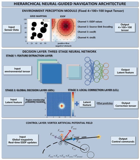
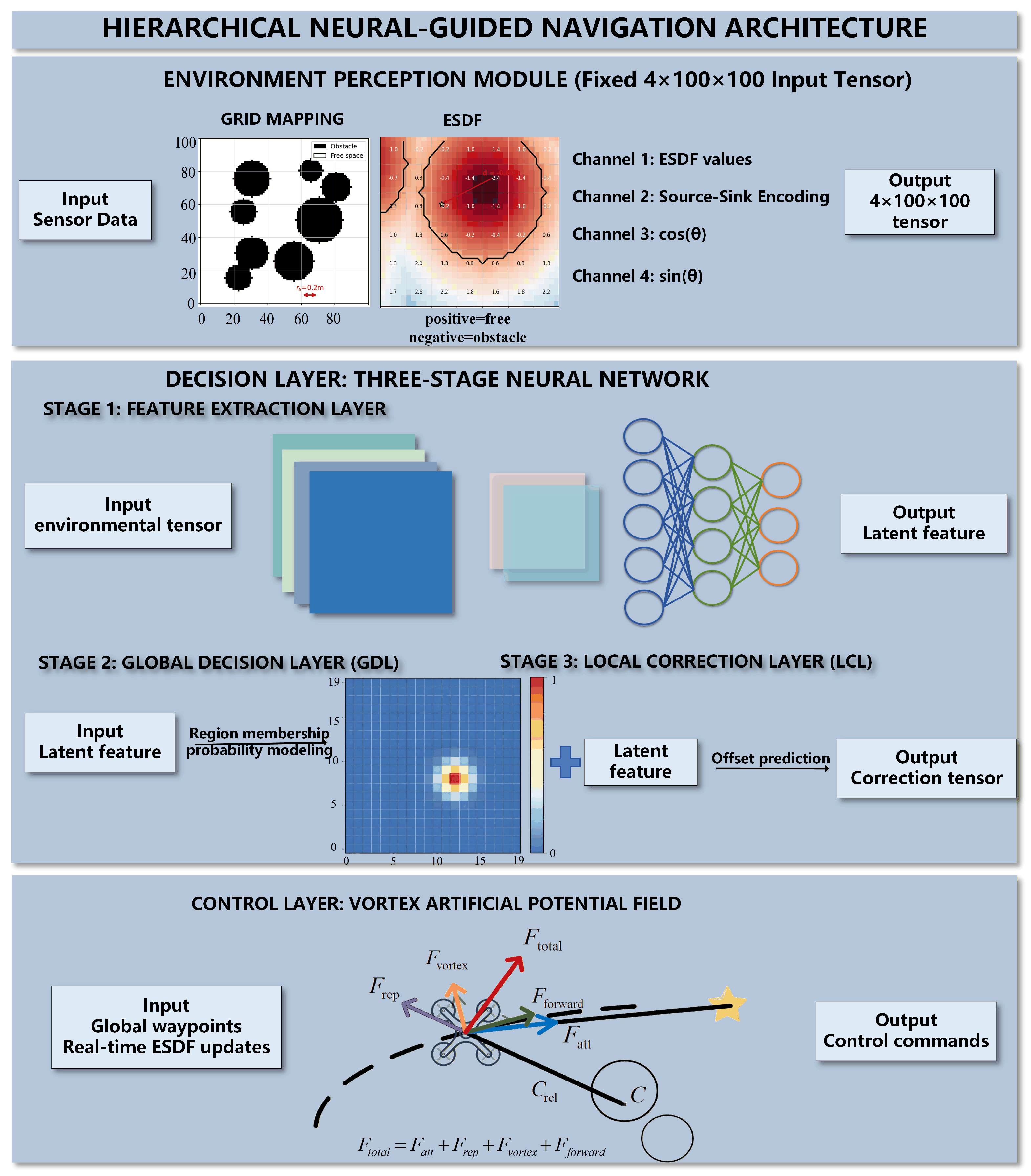
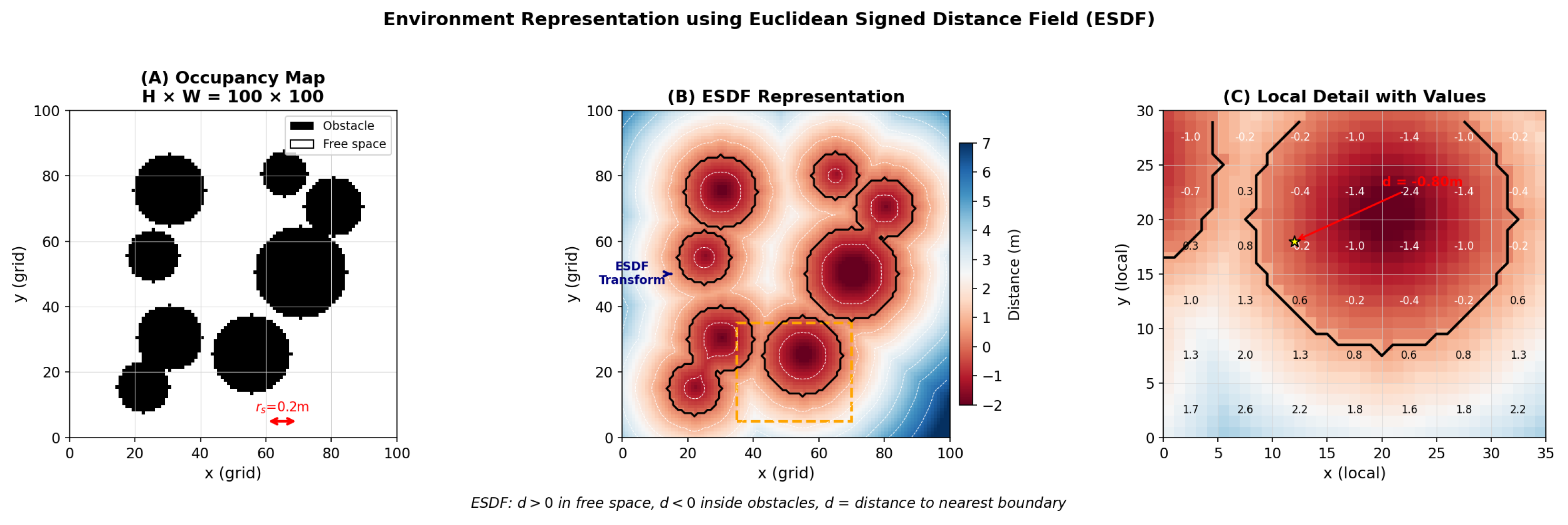
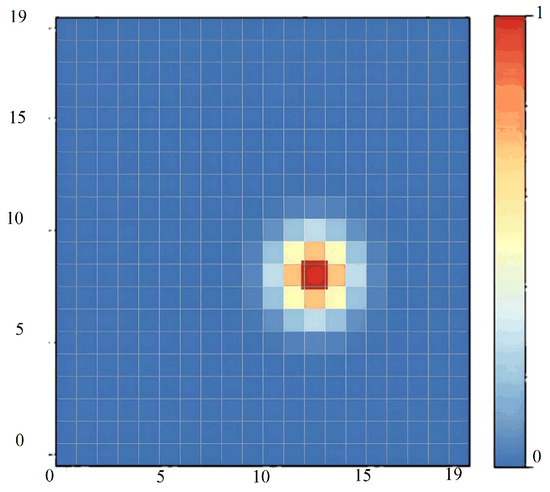
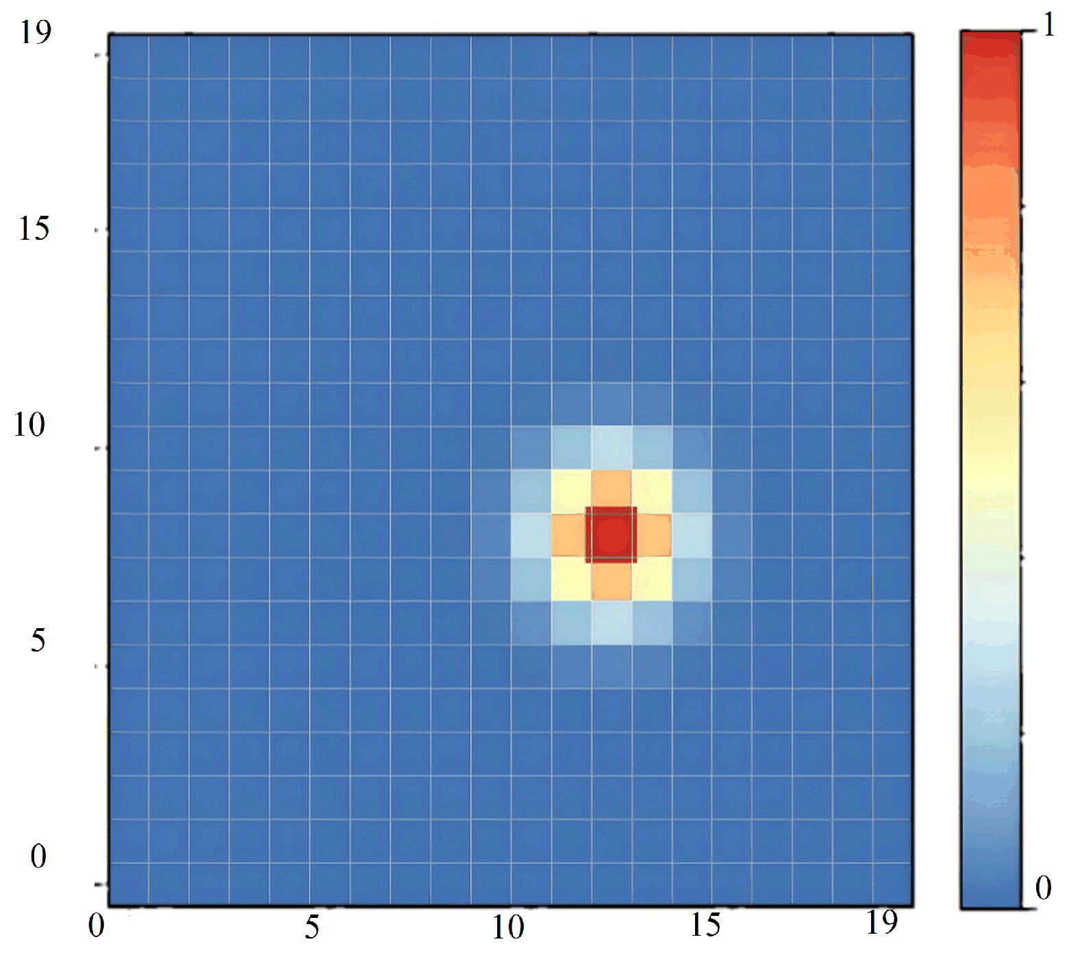
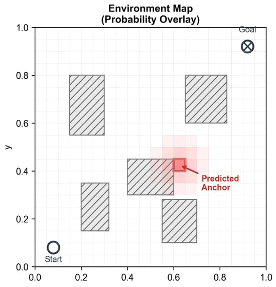
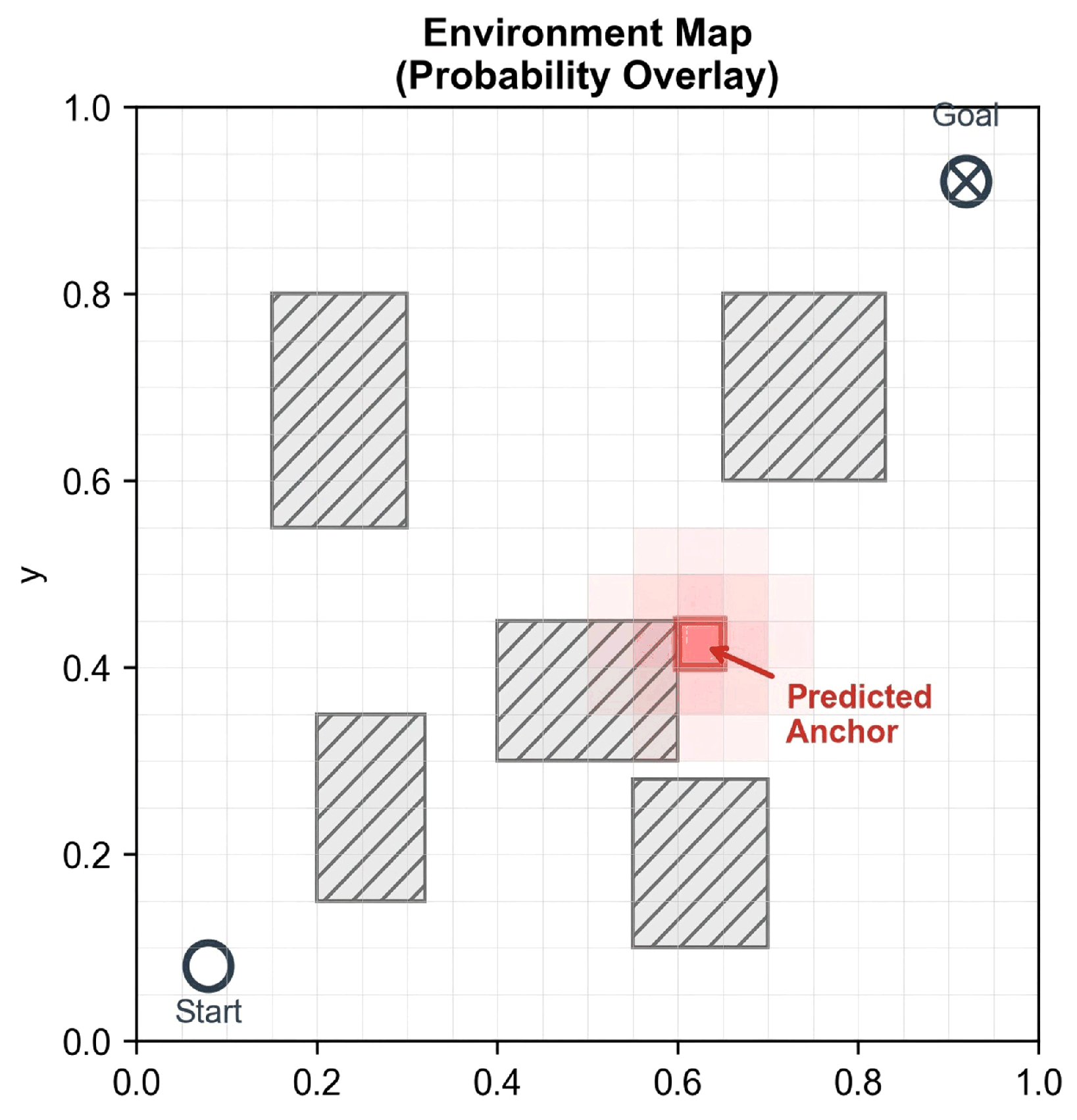
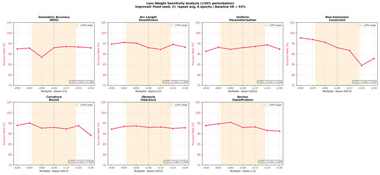
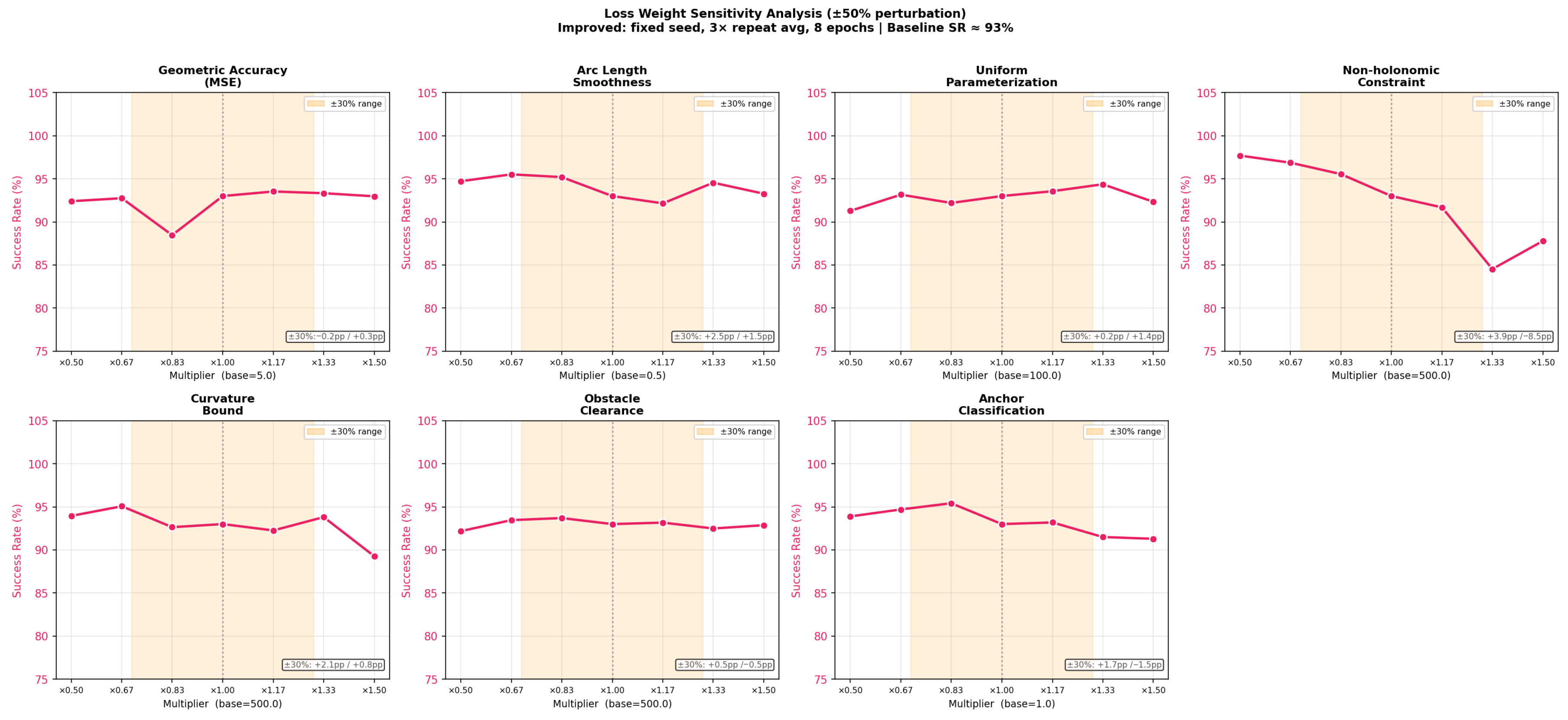
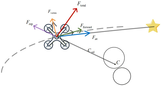
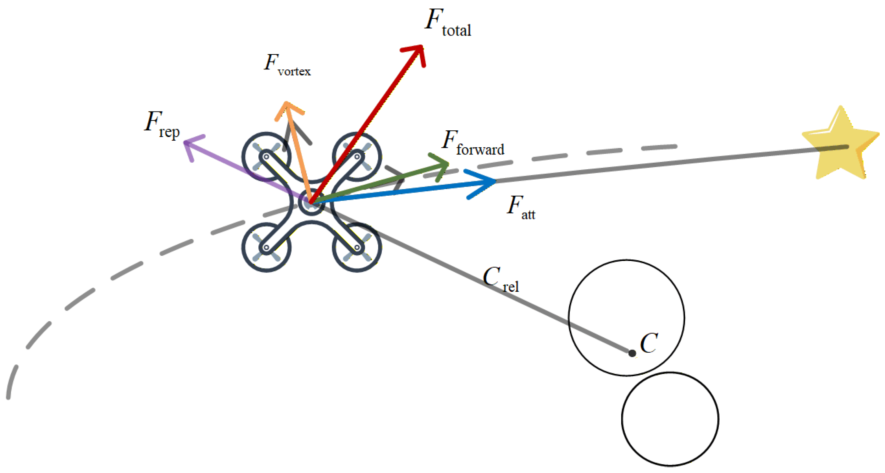
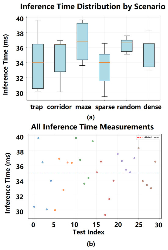
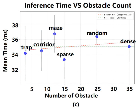
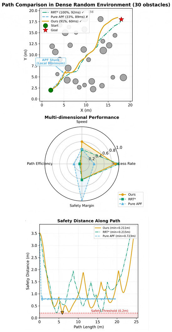
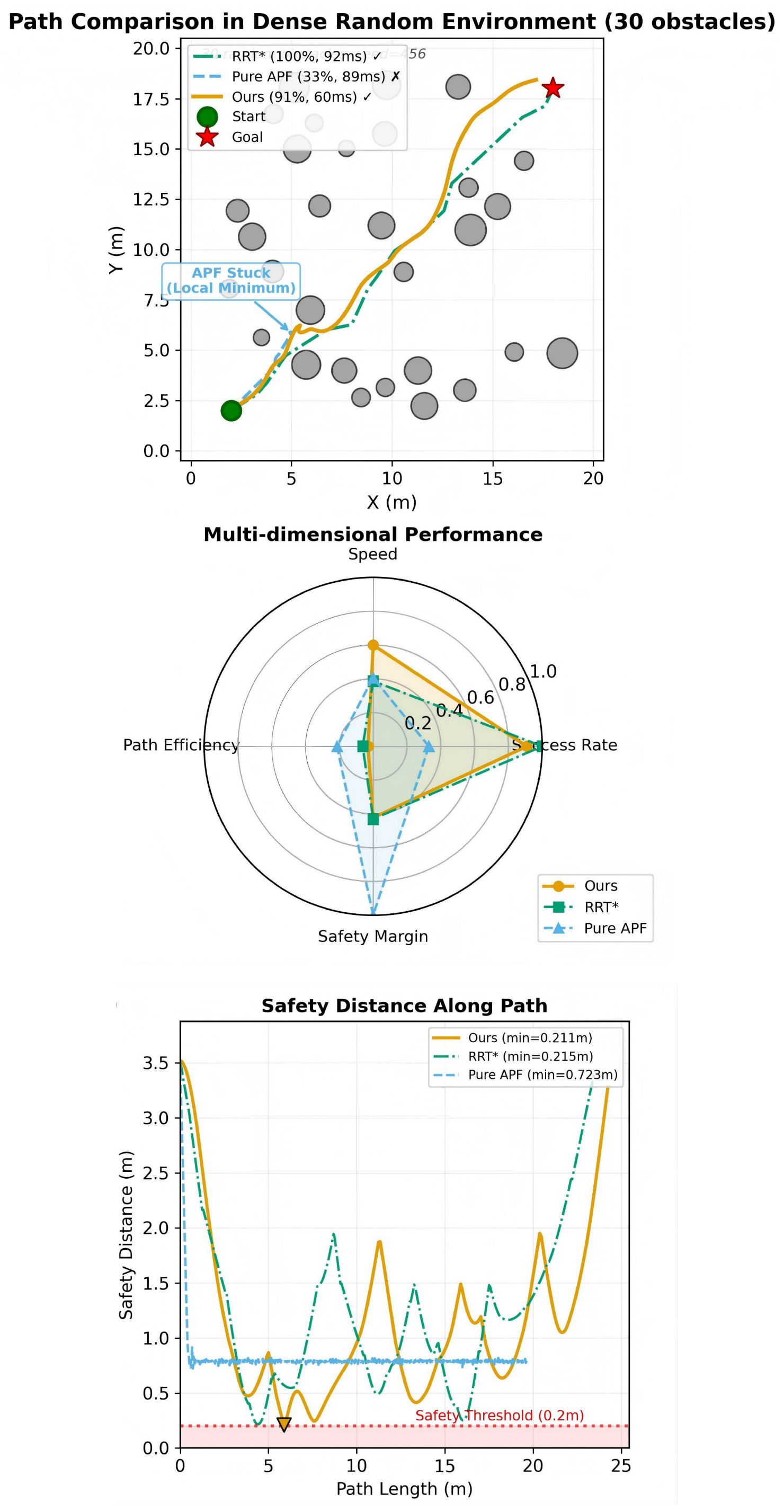
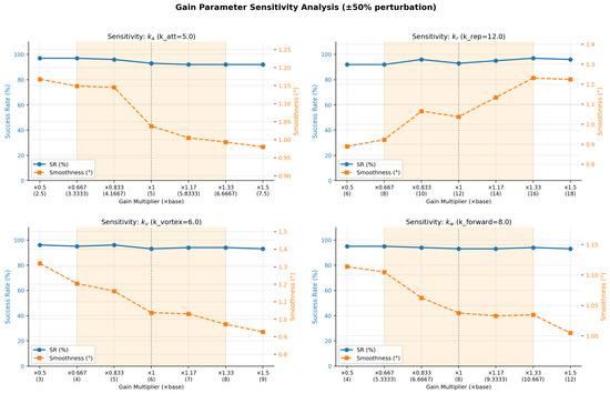
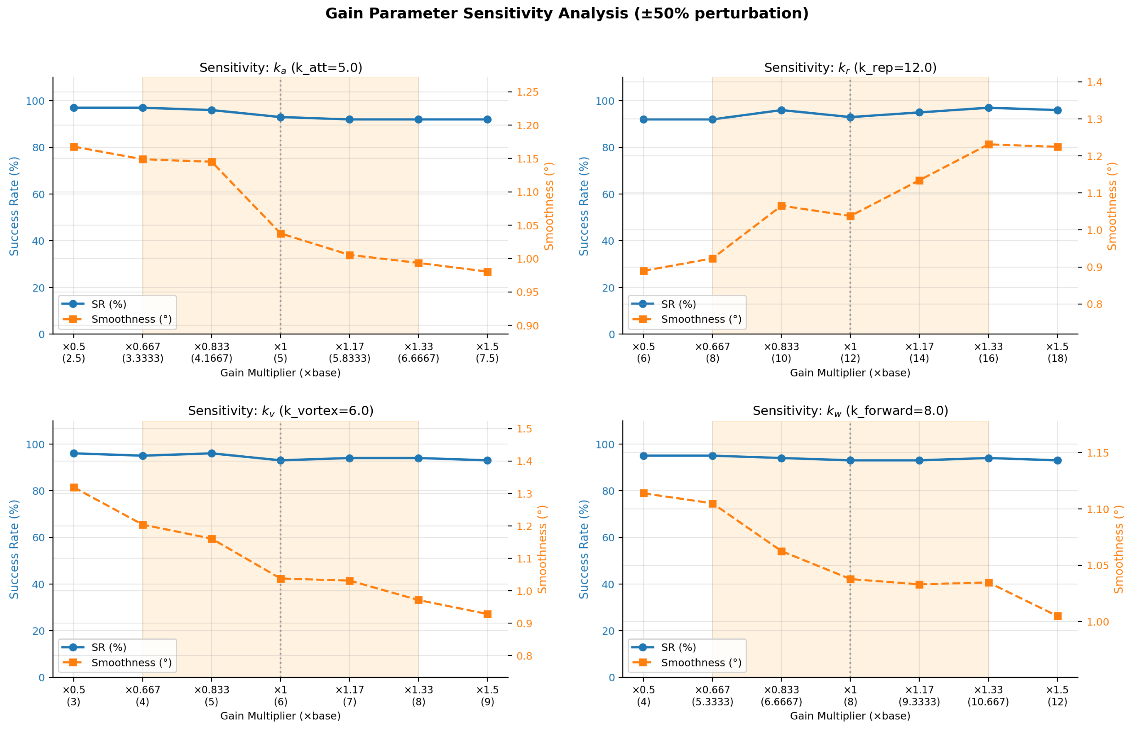

Disclaimer/Publisher’s Note: The statements, opinions and data contained in all publications are solely those of the individual author(s) and contributor(s) and not of MDPI and/or the editor(s). MDPI and/or the editor(s) disclaim responsibility for any injury to people or property resulting from any ideas, methods, instructions or products referred to in the content. |
© 2026 by the authors. Licensee MDPI, Basel, Switzerland. This article is an open access article distributed under the terms and conditions of the Creative Commons Attribution (CC BY) license.