


Highlights
What are the main findings?
- A dynamic coefficient adaptation mechanism that adjusts attractive, repulsive, and trajectory-guidance terms according to target distance, obstacle distance, obstacle density, and path curvature.
- A complete gradient-based control law enabling the algorithm to directly generate UAV-executable motion commands.
What are the implications of the main findings?
- This enables drones to perform tasks more quickly and efficiently in complex environments.
- Be able to better adapt to the environment and complete search and rescue tasks in various environments.
Abstract
This paper presents an adaptive UAV path planning algorithm, A*-APF, which combines the A* algorithm with the artificial potential field method (APF) to overcome challenges such as lengthy paths, lack of smoothness, and local optima in traditional path planning algorithms within intricate environments. The A*-APF algorithm utilizes the global heuristic search abilities of A* and integrates a dynamic adaptive mechanism for gravitational and repulsive coefficients based on target distance, obstacle density, and path curvature. This mechanism enables real-time adjustments of potential field parameters, improving both global optimality and local path smoothness. Simulation results demonstrate that the A*-APF algorithm surpasses A*, RRT, PRM, and GWO algorithms in terms of path length, smoothness, computational efficiency, and stability. Specifically, it reduces the average path length by 15–25%, enhances smoothness by 30–45%, and decreases computation time by nearly 90%. Physical experiments confirm that the algorithm achieves the shortest path, optimal obstacle avoidance, and superior stability in real-world environments, highlighting its global optimization capability, real-time performance, and potential for engineering applications in complex dynamic environments. These results emphasize the algorithm’s ability to enhance UAV stability during task execution.
1. Introduction
In recent years, Unmanned Aerial Vehicle (UAV) technology has been extensively utilized in diverse fields such as environmental monitoring, disaster search and rescue, precision agriculture, and urban logistics due to its flexibility, rapid deployment, and cost efficiency. As the complexity of application scenarios increases, UAVs are required to autonomously devise paths and maneuver around obstacles in unfamiliar or changing environments [1,2,3]. The performance of path planning algorithms directly affects flight safety, mission efficiency, and energy conservation, making the development of high-precision, robustness, and real-time path planning algorithms of both theoretical significance and practical engineering value [4,5].
With the growing demand for autonomous navigation and obstacle avoidance in UAVs rises, researchers both domestically and internationally have proposed various improvements and fusion algorithms, which can be broadly categorized into three major technical frameworks: graph search algorithms, sampling-based algorithms, and intelligent optimization algorithms [6]. Notably, the A* (A-Star) algorithm stands out as one of the most representative heuristic global search methods. By considering path length and distance to the goal, A* can efficiently identify a near-optimal path in a discretized environment. Its advantages include stable search results, high repeatability, strong global optimality, and ease of integration with map information for global planning. However, when the search space has high dimensionality or dense obstacles, the number of expanded nodes grows exponentially, resulting in reduced computational efficiency. Additionally, the paths generated by A* consist of discrete nodes, lacking smoothness and dynamic feasibility, and fail to be directly applied to continuous UAV control systems [7,8,9].
To enhance real-time performance and scalability, researchers have introduced path planning techniques centered on random sampling, such as Probabilistic Roadmap (PRM) and Rapidly-exploring Random Tree (RRT) [10,11,12]. PRM generates a sparse connected graph model by sampling nodes in free space and linking feasible edges with collision detection constraints, enabling rapid depiction of high-dimensional space topology for offline global planning. Nonetheless, PRM exhibits limited adaptability to environmental variations, necessitating resampling and remapping upon changes in obstacle position or shape, limiting its real-time applicability. The RRT algorithm dynamically expands towards unexplored regions utilizing a random tree structure, facilitating swift identification of viable paths in intricate spaces [13,14,15,16,17]. Variants such as RRT* and Informed-RRT* improve search efficiency and feasibility but still suffer from long and non-smooth paths, high randomness, frequent path corrections, and substantial computational overhead in dynamic environments, making them less suitable for real-time obstacle avoidance [18,19,20,21].
In addition to graph search and sampling-based methods, population-based metaheuristic optimization algorithms have recently been applied to path planning. The Grey Wolf Optimizer (GWO) simulates the hierarchical and hunting behaviors of grey wolves, achieving both global exploration and local exploitation [22,23,24,25]. While GWO exhibits strong global search capability and stable convergence, it still has limitations for real-time UAV path planning, including difficulties in dynamic environments, complex parameter tuning in high-dimensional spaces, and large computational demands [26]. In contrast, the Artificial Potential Field (APF) method models the UAV’s motion using attractive and repulsive forces derived from the goal and obstacles, generating control commands directly. APF does not require discrete node searches or complex graph structures and performs real-time path generation and obstacle avoidance in continuous space with low computational cost and straightforward implementation [27]. However, traditional APF suffers from local minima, unreachable goals, and fixed parameter settings, which limit its performance in complex environments.
To overcome these limitations, recent studies have proposed hybrid algorithms that integrate global optimization and local obstacle avoidance. For instance, reference [28] combined RRT* and APF for robotic arm path planning, improving sampling efficiency, runtime, and path length; reference [29] developed a collaborative avoidance algorithm integrating formation potential fields and dynamic omnidirectional disturbance fields, enhancing trajectory planning success rate and robustness; reference [30] proposed an adaptive potential field method to improve UAV obstacle avoidance. Nevertheless, these hybrid approaches still have shortcomings due to the inherent limitations of the basic algorithms. PRM-APF methods guide APF using PRM’s global connectivity, while GWO-APF uses population intelligence to adjust potential field parameters for global search, but the coupling between global planning and local adjustment remains insufficient [31]. Population-intelligence-based APF hybrids could optimize potential-field parameters, but they typically rely on offline or batch optimization and introduce additional computational overhead. Their integration into real-time UAV navigation systems therefore remains challenging, especially in dynamic or resource-constrained settings [32,33,34,35].
The main novelty of this work is an A*-guided adaptive APF framework that converts a discrete global plan into UAV-executable continuous motion commands. Concretely, the proposed method contributes are as follows:
(1) A state-driven coefficient adaptation that jointly tunes attraction, repulsion, and trajectory-adherence terms using goal distance, obstacle proximity/density, and path curvature;
(2) An A*-derived reference integration that introduces a trajectory-guidance potential into a fused potential well, bridging discrete global planning and continuous local control;
(3) A cost-function-based online self-tuning mechanism that refines parameters during navigation under bounded feasibility constraints;
(4) A unified gradient-based control law that directly produces continuous commands for execution.
Unlike PRM-APF or RRT*-APF hybrids that primarily use sampling-based global connectivity to guide a local APF, and unlike population-intelligence-APF methods that mainly optimize APF parameters offline or at a higher computational cost, our method emphasizes low-frequency, global guidance + per-cycle local constant-complexity updates, improving executability and real-time robustness without claiming strict global optimality proofs.
This paper presents an adaptive UAV path planning algorithm that integrates A* and Artificial Potential Fields (APF), referred to as A*-APF, leveraging the global optimality of A*. The algorithm utilizes A* for global planning while employing APF for local obstacle avoidance. It introduces a dynamic adjustment mechanism for the attractive and repulsive coefficients, enabling the potential field parameters to adapt to the UAV’s state and the surrounding environment. This approach facilitates globally feasible, locally smooth, and efficient path planning. The proposed algorithm successfully achieves global path optimization, local stability, and effective obstacle avoidance in complex dynamic environments, thereby providing a real-time, reliable solution for autonomous UAV navigation. Table 1 summarizes the comparison of closely related adaptive APF and hybrid planning methods. Table 2 summarizes the definitions of the variables used in this paper.
Table 1.
Comparison with closely related adaptive APF and hybrid planning methods.
Table 2.
The definitions of the variables used in this article.
2. Theoretical Foundations of Algorithms
This section presents the methodology of the proposed adaptive path planning algorithm that integrates the A* algorithm with an Artificial Potential Field (APF) framework. Unlike conventional approaches that separately emphasize global optimality or local real-time control, the proposed A*-APF algorithm aims to achieve global feasibility, local smoothness, and adaptive robustness through a unified design. The A* algorithm is employed to provide global structural guidance, while an adaptive APF with state-dependent parameters generates continuous and executable UAV motion commands.
2.1. Global Reference Path Generation Using A*
The A* algorithm is adopted in this work as a global reference planner to generate a collision-free path from the start position to the target in a discretized environment. Its purpose is not to directly control the UAV, but rather to provide global topological guidance for subsequent local trajectory generation.
In the A* framework, each node is evaluated by the standard cost function.
where denotes the accumulated cost from the start node to the current node, and represents a heuristic estimate of the remaining cost to the goal. This formulation enables efficient global search while maintaining near-optimality under commonly used heuristic functions.
The theoretical properties of the A* algorithm, such as heuristic admissibility, consistency, and optimality guarantees, have been extensively investigated in the literature and are therefore not reiterated in this paper. Instead, the emphasis is placed on how the A* output is utilized within the proposed framework. At each step, the algorithm selects the node with the smallest for expansion until the goal node is reached. A schematic diagram of the overall algorithm is shown in Figure 1. In the figure, “a, b, c, d, e, f, z” represent the various points that the route might pass through from the starting point to the destination. Among them, “a” is the starting point and “z” is the destination. The red line segment in the picture represents the path that the unmanned vehicle has taken from the starting point to the end point. The algorithm enables the UAV to successfully reach the goal while avoiding these obstacles.
Figure 1.
Schematic diagram of A* algorithm path planning.
Specifically, the discrete path produced by A* is interpolated into a continuous reference trajectory. This trajectory is not rigidly enforced but is incorporated into the potential field formulation as a trajectory guidance term, allowing the UAV to follow the global path structure while retaining flexibility for local obstacle avoidance. This design effectively bridges the gap between global planning and continuous real-time control.
The output of the A* algorithm is a discrete sequence of grid nodes, which cannot be directly executed by a UAV due to discontinuities and abrupt heading changes. Therefore, the discrete A* path is converted into a continuous reference trajectory prior to integration with the APF framework.
Specifically, the sequence of A* waypoints is first pruned to remove collinear nodes, and then interpolated using a cubic spline interpolation to generate a C1-continuous reference curve. This interpolation preserves the global topological structure of the A* path while smoothing sharp turns introduced by grid discretization. The resulting reference trajectory is used solely as a soft global guidance signal rather than a hard constraint, allowing the UAV to deviate locally when necessary for obstacle avoidance.
2.2. Artificial Potential Field Framework
The Artificial Potential Field (APF) method, originally proposed by Oussama Khatib in 1985, is a classical path planning algorithm. Its core idea is to model the robot’s motion in space as the result of combined attractive and repulsive forces: the goal generates an attractive force that pulls the robot toward it, while obstacles generate repulsive forces that prevent the robot from approaching them. Consequently, the robot’s trajectory can be regarded as the path along the direction of decreasing potential in this artificial potential field. The Artificial Potential Field (APF) method is employed as the local motion planning and control framework due to its low computational complexity and suitability for real-time UAV applications. In the classical APF formulation, the UAV motion is governed by the superposition of attractive and repulsive potentials.
The total potential function is defined as
where represents the attractive potential generated by the target, and represents the repulsive potential generated by surrounding obstacles.
The attractive potential is defined as
And the attractive potential is defined as
where and denote the attractive and repulsive coefficients, respectively. Although APF provides continuous and computationally efficient path generation, its performance is highly sensitive to parameter selection. Fixed attractive and repulsive coefficients often lead to local minima, oscillations, and poor adaptability in environments with varying obstacle density and mission stages. These limitations motivate the introduction of adaptive mechanisms in the proposed framework. Figure 2 shows a two-dimensional schematic of the Artificial Potential Field method.
Figure 2.
APF Algorithm Flowchart.
The black dot at the center of the figure represents the current position of the robot, labeled as p. The attractive force is generated by the goal, pointing toward the goal, and indicated by a dashed arrow. The repulsive force is generated by obstacles, pointing away from the obstacles, and represented by a solid red or black arrow. The resultant force indicates the final direction of force acting on the robot within the artificial potential field, corresponding to the robot’s next movement direction.
2.3. Summary
Although the Artificial Potential Field (APF) method has been extensively employed for UAV and mobile robot path planning due to its conceptual simplicity, computational efficiency, and intuitive physical interpretation, it exhibits several inherent limitations in complex environments. A prominent issue is the local minima problem: when attractive and repulsive forces equilibrate, the UAV may become trapped at a non-goal local equilibrium point, thereby halting progress toward the target.
A further limitation arises from the fixed nature of APF parameters, including the attractive and repulsive coefficients, as well as the sensing radius. The algorithm’s performance is highly sensitive to these parameters; in environments with varying complexity or obstacle density, static parameter settings cannot adapt dynamically, which may result in either excessive avoidance—causing oscillatory trajectories or deviation from the optimal path—or insufficient avoidance, increasing the risk of collisions in proximity to obstacles.
Additionally, in narrow passages or multi-obstacle scenarios, APF often induces oscillatory behavior, whereby the UAV repeatedly traverses between adjacent obstacle potential boundaries without achieving stable passage. Conventional APF formulations typically consider only the spatial relationships between the goal and obstacles, neglecting the vehicle’s dynamic constraints and path smoothness requirements. This limitation may yield physically infeasible trajectories or result in abrupt control input variations.
Finally, as a fundamentally local planning method, APF lacks global environmental awareness, rendering it challenging to ensure global optimality and path reachability. Consequently, while traditional APF offers advantages in terms of real-time computation and straightforward implementation, its robustness and stability in complex, dynamic environments remain limited. Contemporary improvements focus on integrating global path planning information and adaptive parameter tuning mechanisms to enhance algorithmic performance in challenging scenarios.
3. Adaptive Path Planning Algorithm Integrating A* and APF with Dynamic Attractive and Repulsive Coefficients
3.1. Adaptive Mechanism for Dynamic Attractive and Repulsive Coefficients
3.1.1. Design Concept
In conventional APF, the attractive coefficient , repulsive coefficient and path adherence coefficient are typically set as fixed constants, tuned only once at the beginning of the simulation based on experience. This approach may work in static environments with sparse obstacles and a single target; however, practical UAV flight missions involve environments with the following characteristics: (1) The distance to the target constantly changes: a strong attractive force is needed when the UAV is far from the goal, whereas maintaining a large attraction when approaching the target may cause overshoot or collisions. (2) Obstacles are distributed non-uniformly in space: stronger repulsive forces are required in dense obstacle regions, while overly conservative forces are unnecessary in open areas. (3) The UAV’s own state varies: at high speeds or along paths with large curvature, excessive attractive or repulsive forces may induce overly aggressive control inputs.
Hence, , , needs to be designed as a state-dependent dynamic parameter, that is: , , . The system “state” may encompass variables such as the distance to the goal , the distance to the nearest obstacle , the local obstacle density , the path curvature , and the UAV velocity .
3.1.2. Construction of Environmental State Variables
To ensure that the adaptive law maintains bounded input variables and preserves physical interpretability, the measured quantities are first normalized.
(1) Normalization of the Goal Distance
Here, is the scaling factor.
When , ; When , .
(2) Normalization of the Distance to the Nearest Obstacle
Let the sensing radius be , and the safety distance be , with
When , , indicating a “dangerous” state; when , , indicating a “safe” state;
(3) Normalization of Obstacle Density
Let denote the obstacle points, then
where ; is the neighborhood centered at the UAV with radius , and is the maximum allowable number of obstacles used for normalization.
3.1.3. Sigmoid-Based Adaptive Law
The Sigmoid-based adaptive law is a parameter adjustment approach grounded in the characteristics of the S-shaped Sigmoid function. It has been widely applied in fields such as intelligent control, path planning, and adaptive potential field algorithms. The fundamental concept is to exploit the smoothness, monotonicity, and boundedness of the Sigmoid function within its input domain to achieve gradual and state-dependent parameter adaptation. Here, the system parameters (e.g., the distance between the UAV and the target, obstacle density, or error magnitude) are adjusted progressively according to the current state variables.
In the improved Artificial Potential Field (APF) algorithm, this adaptive law is typically employed to dynamically modify the attractive and repulsive coefficients, enabling the potential field intensity to vary with environmental changes in a nonlinear rather than linear manner. When the UAV approaches either obstacles or the target, the Sigmoid function ensures a smooth variation in the potential field magnitude, allowing the UAV to escape from local minima and oscillations more effectively, while enhancing the stability, intelligence, and convergence performance of the path planning process.
To ensure that the coefficient variations remain smooth, controllable, and bounded within explicit upper and lower limits, the following Sigmoid mapping is adopted:
where .
(1) Adaptive Adjustment of the Attractive Coefficient
When the UAV is far from the target, a stronger attractive force is desired; however, in regions with dense obstacles, the attraction should be moderately suppressed. Thus, the coefficient can be designed as:
When , the attraction increases with distance from the target; when , higher obstacle density reduces the attraction, preventing the UAV from being “pulled” into obstacle clusters; when , larger path curvature leads to a smaller attraction, mitigating sharp turns.
(2) Adaptive Adjustment of the Repulsive Coefficient
When the UAV approaches obstacles or when obstacle density increases, the repulsive force should be promptly amplified:
Here, controls sensitivity to the nearest obstacle distance, controls sensitivity to the overall obstacle density, and allows the repulsive force to slightly increase in regions of high curvature, preventing edge-following flight.
(3) Adaptive Adjustment of the Trajectory Adherence Coefficient (A*-Integrated)
When the environment is densely populated with obstacles, the UAV should adhere closely to the global path generated by A*; conversely, in open areas, this constraint can be appropriately relaxed:
Through these formulations, a rule-based adaptive law is obtained.
3.1.4. Cost-Function-Based Online Optimization for Parameter Self-Tuning
While the Sigmoid-based adaptive law provides an efficient rule-driven way to adjust the potential-field coefficients according to the UAV–goal distance, obstacle proximity, obstacle density, and path curvature, the selection of its functional form and weighting factors is largely empirical. Therefore, similar to most adaptive APF variants reported in the literature, such strategies typically do not provide explicit theoretical guarantees of global optimality or Lyapunov-based convergence in complex and dynamic environments. In this work, the purpose is not to claim strict global optimality, but to improve practical robustness and stability under real-time constraints.
To further reduce dependence on manual parameter tuning, we introduce a cost-function-based online optimization mechanism for parameter self-tuning. Importantly, this mechanism is not a data-driven learning method (e.g., supervised learning or reinforcement learning), since it does not rely on an external training dataset or a learned model. Instead, it performs a lightweight online refinement of the parameter vector by minimizing a task-related cost defined from the current planning/control status.
A directional cost function can first be defined as:
where indicates activation only when the UAV approaches obstacles.
The parameters can then be fine-tuned through a gradient-descent update rule:
Followed by a projection constraint that maps the parameters back into their feasible range:
This online optimization step serves as a performance-driven self-tuning process: it incrementally adjusts the coefficients to reduce the instantaneous task cost while maintaining feasibility through bounded constraints. Although this approach does not establish a strict analytical convergence proof, it improves robustness in practice by (1) preventing unbounded parameter drift via projection constraints, and (2) refining parameter values according to objective performance indicators during navigation. The effectiveness and stability of the proposed self-tuning mechanism are therefore demonstrated through extensive simulations and physical experiments, rather than formal theoretical guarantees.
Note that oscillations in APF-based navigation are typically caused by abrupt switching of gains or noisy distance measurements. The proposed update is rate-limited and bounded, and the control command is damped and saturated, which together mitigate oscillatory behaviors.
To isolate the contribution of the proposed adaptation strategy, we distinguish two levels of adaptivity in A*-APF: (i) a rule-driven, state-dependent Sigmoid mapping that modulates coefficients according to goal distance, obstacle proximity/density, and path curvature; and (ii) a cost-function-driven online self-tuning step that incrementally refines the parameter vector via bounded gradient updates with projection constraints. While both mechanisms are adaptive, they play distinct roles: the Sigmoid mapping provides immediate and interpretable gain modulation for real-time responsiveness, whereas the online self-tuning further reduces manual parameter dependence and compensates for modeling mismatch across heterogeneous environments. Accordingly, we perform a targeted ablation by comparing A*-APF without online self-tuning (Sigmoid adaptation only) and the full A*-APF, which explicitly reveals the incremental benefit of self-tuning in terms of path length and detour reduction in cluttered regions, curvature smoothness and oscillation suppression in narrow passages, and improved stability across repeated trials. This controlled baseline also establishes a fair reference for comparison with other adaptive APF variants, which typically rely solely on heuristic gain scheduling, while the proposed framework incorporates a lightweight, performance-driven refinement that remains online, bounded, and suitable for real-time execution.
3.1.5. Online Update Stabilization and Safety Mechanisms
The gradient-based online parameter update in Equations (12)–(14) is designed as a lightweight self-tuning step rather than a full learning process. Since online updates may introduce transient parameter variations, the following stabilization and safety mechanisms are adopted to prevent oscillations and unsafe behaviors in dynamic environments.
(1) Boundedness via projection. The parameter vector is projected onto predefined feasible intervals, which prevents unbounded drift and guarantees that the attractive/repulsive/trajectory-adherence gains remain within physically meaningful ranges.
(2) Conservative step size selection. The learning rate is chosen to be sufficiently small to ensure gradual parameter evolution relative to the control cycle. In our implementation, is tuned such that the relative change in each gain per update is limited (e.g., below a small percentage of its current value), avoiding abrupt changes in control commands.
(3) Update rate limiting and smoothing. To reduce sensitivity to measurement noise and environmental fluctuations, parameter refinement is performed at a lower frequency than the control loop (e.g., every control cycles), and the updated gains are optionally filtered using a first-order smoothing strategy. This prevents high-frequency gain switching and mitigates oscillatory behavior.
(4) Safety-guarded update and command saturation. During online navigation, safety constraints are enforced through (1) acceleration/velocity saturation in the control layer, and (2) a guarded update policy: when the UAV is within a near-obstacle safety region, repulsion-dominant settings are prioritized and parameter updates that would reduce safety margins are rejected. This ensures that transient parameter changes do not lead to unsafe commands.
With these mechanisms, the online update remains stable in practice, and the algorithm maintains safe behavior during transient parameter variations. The effectiveness of these safeguards is validated empirically in the simulation and physical experiments.
3.2. Unified Model Integrating A* and APF
In the conventional A* algorithm, the generated path is globally optimal but inherently discrete, making it unsuitable for directly driving a continuous UAV trajectory. In contrast, the traditional Artificial Potential Field (APF) algorithm offers continuous control but only achieves local optimality, often suffering from local minima and high sensitivity to parameter settings.
To overcome these limitations, a unified model is proposed that integrates the strengths of both algorithms to achieve superior path planning performance. The core idea is to combine the two frameworks at the initialization level: the discrete path obtained from A* is transformed into a continuous reference trajectory through spline interpolation. The deviation from this reference trajectory is then treated as a form of “potential energy,” which is incorporated into an augmented potential function alongside the goal attraction and obstacle repulsion terms. It should be emphasized that the interpolated A* reference trajectory is generated once (or updated at low frequency when replanning is triggered) and is embedded into the potential-field formulation as a guidance term, rather than being applied as a post-processing smoothing step to the final trajectory.
Construction of the Augmented Potential Function
First, the fused potential function is defined as:
Here, denotes that the endpoint of A* serves as the goal for APF; represents the native obstacle repulsion in APF; corresponds to the “global reference trajectory adherence” provided by A*. Here , which indicates the current nearest position on the trajectory. To achieve a smoother trajectory, the following equation can be incorporated:
The final result is obtained as:
3.3. The Explicit Forms of the Gradient and the Control Law
3.3.1. Goal Term Gradient
In general implementations, is often neglected (since it originates from the adaptive law and varies slowly); thus
3.3.2. Obstacle Term Gradient
Denote , as
Substituting into , it can be concluded
The contributions of multiple obstacles are summed.
3.3.3. Trajectory Attraction Gradient
Thus, the total gradient is given by
The control law is selected as the negative gradient with damping:
Equation (25) is expanded as follows:
The flowchart of the algorithm is shown in Figure 3, which clearly and concisely illustrates the general process of combining the two algorithms and summarizes the above derivation process. To make it easier to understand, the pseudo-code of the relevant algorithm is shown as Algorithm 1.
| Algorithm 1. A*-APF Planning and Control Pipeline |
| Input: Start position p_s Goal position p_g Obstacle set O UAV initial state x_0 Planning parameters Θ Output: Continuous control commands u(t) /* Global reference generation */ Compute a discrete global path P_A* using the A* algorithm Generate a continuous reference path P_ref by spline interpolation of P_A* /* APF initialization */ Initialize attractive, repulsive, and trajectory-adherence coefficients Initialize adaptive parameter vector θ within predefined bounds /* Online navigation and control loop */ while goal is not reached do Acquire current UAV state x(t) Obtain obstacle distance information d_o(t) /* Adaptive coefficient update */ Update APF coefficients using state-driven mapping Refine parameters via cost-function-based online self-tuning /* Potential-field evaluation */ Compute attractive, repulsive, and reference-guidance potentials Fuse potentials to obtain total potential field /* Control computation */ Compute control command u(t) using gradient-based control law Apply saturation and feasibility constraints /* State propagation */ Update UAV state x(t + 1) via numerical integration end while if reference becomes obstructed or tracking error exceeds threshold then re-run A* to update P_ref (low-frequency replanning) end if |
Figure 3.
Flowchart of the Improved Integrated Algorithm.
3.4. UAV Motion Model and Numerical Integration
In the simulation studies, the UAV is modeled using a simplified point-mass kinematic model, which is commonly adopted in path planning and obstacle avoidance research. The UAV state vector is defined as
where and denote the position and velocity of the UAV, respectively.
The control input u(t) generated by the proposed A*-APF algorithm corresponds to a virtual acceleration command derived from the negative gradient of the total potential field with damping. The UAV motion is numerically updated using a discrete-time integration scheme:
where is the simulation time step. Velocity and acceleration limits are enforced to ensure numerical stability and physical feasibility.
This kinematic formulation enables continuous trajectory generation while maintaining low computational complexity, and it is sufficient for evaluating the planning and obstacle avoidance behavior of the proposed algorithm.
In the simulation studies, the UAV is modeled using a simplified point-mass kinematic model, which is widely adopted in path planning and obstacle avoidance research to evaluate navigation behavior independently of low-level flight control dynamics.
The UAV state is defined by its position and velocity vectors in Cartesian space. The control input generated by the proposed A*-APF algorithm corresponds to a virtual acceleration command derived from the gradient of the total potential field combined with a damping term.
At each discrete simulation step, the UAV state is updated through time discretization with a fixed integration step size. Specifically, the velocity is first updated according to the computed control input, and the position is then propagated using the updated velocity. This numerical integration scheme enables the generation of continuous trajectories from the proposed algorithm while maintaining computational efficiency.
To ensure numerical stability and physical feasibility, velocity and acceleration limits are imposed during the simulation. These constraints prevent excessive control inputs and unrealistic motion behavior while preserving the qualitative characteristics of the planned trajectory.
This kinematic modeling approach provides a consistent and reproducible framework for evaluating the global planning and local obstacle avoidance performance of the proposed algorithm in complex environments.
4. Simulation Validation
The previous sections have presented the formulation and implementation of the proposed A*-APF algorithm. This section focuses on simulation-based validation and comparative evaluation in complex environments.
It should be emphasized that the algorithms considered in this study operate at different planning and execution levels. The A* algorithm is a discrete global path planner, whose primary objective is to ensure global feasibility and near-optimal path length in a grid-based search space. It outputs a sequence of discrete waypoints and is not designed to directly generate smooth or dynamically feasible trajectories. In contrast, the proposed A*-APF algorithm, as well as APF-based and sampling-based methods, produce continuous trajectories suitable for direct execution by UAVs.
Therefore, the comparative evaluation is conducted in a hierarchical manner. Specifically, A* is mainly evaluated in terms of global planning performance, including path feasibility, path length, and computational efficiency. Metrics related to trajectory smoothness, curvature, and motion continuity are primarily used to compare methods that inherently generate continuous trajectories. Smoothness-related results involving the original A* algorithm are reported for reference purposes only, rather than as a primary performance indicator.
Based on this evaluation framework, the proposed A*-APF algorithm is compared with traditional A* algorithm, Grey Wolf Optimizer (GWO), Probabilistic Roadmap (PRM), and Rapidly-exploring Random Tree (RRT)under identical environmental settings. The comparison aims to assess both global planning effectiveness and practical trajectory execution performance in complex environments.
Furthermore, real-world experiments are carried out on a self-developed UAV platform to verify the feasibility and effectiveness of the algorithm in practical operating environments, thereby enhancing its credibility and applicability in engineering applications.
4.1. Simulation Settings
The overall simulation experiments were all conducted in MATLAB R2022b. In this simulation scenario, the green five-pointed star serves as the starting point, while the yellow and red five-pointed stars represent the endpoints, the environment is defined as 200 m × 200 m area with the start point located at (0 m,0 m,0 m), and the target points are set at (200 m, 200 m, 0 m) and (300 m, 300 m, 0 m). The weight parameter is set to 0.4, and the population size for all three comparison algorithms is fixed at 50. Cylindrical obstacles are randomly generated with varying heights. To accurately simulate obstacles suspended in the air in a real environment, some of the cylindrical bodies do not touch the ground at their bases, in order to better validate the algorithm. A total of 100 random trials is conducted within the defined environment. The online refinement uses a small learning rate (set within the range of in our experiments) and is executed every control cycles (e.g., ). We report the full set of baseline parameters and tested ranges in Table A1 and Table A2 (Appendix A). In addition, velocity and acceleration commands are saturated to predefined limits to ensure physical feasibility. The following section presents the simulation results and provides a detailed analysis of the experimental outcomes. At each simulation step, the current UAV state is used to compute the attractive, repulsive, and trajectory-guidance coefficients of the potential field. Based on the adaptive coefficients, the control input is updated, and the UAV position is propagated to the next continuous node through numerical integration. This process is repeated iteratively until the target is reached or a termination condition is satisfied. Among them, Figure 4 shows the 3D and 2D simulation results in the two environments.
Figure 4.
Simulation results of the five algorithms: (a) 3D simulation results in a 200 × 200 map; (b) 3D simulation results in a 300 × 300 map; (c) 2D simulation results in a 200 × 200 map; (d) 2D simulation results in a 300 × 300 map.
The simulation and outdoor flight tests in this study primarily consider static or quasi-static obstacles, which is consistent with many practical inspection and navigation scenarios. To address environmental changes and potential sensing delays, the proposed framework operates in a receding-horizon, online manner: obstacle distance measurements and the UAV state are updated at every control cycle, and the local APF-based control command is recomputed accordingly. This provides a reactive avoidance behavior that can respond to changes in obstacle proximity without requiring an explicit obstacle motion model.
The A* module is used only for low-frequency global reference generation (or initialization), while the APF control loop runs at a higher frequency to ensure timely reaction. In our implementation, the control cycle is updated at [20~50 Hz], and the online parameter refinement is executed every M = 5 cycles. If a major environmental change is detected (e.g., the reference path becomes obstructed or the deviation from the reference exceeds a threshold), the global reference can be regenerated by re-running A* at a lower rate.
Regarding sensing latency, the proposed approach does not require precise obstacle dynamics prediction; instead, it relies on frequent state updates, damping, command saturation, and safety margins (e.g., ) to maintain safe behavior under moderate delays. A full prediction-based extension for highly dynamic obstacles is outside the scope of the current study and will be investigated in future work.
Velocity, acceleration, and control-input constraints are imposed to ensure physical feasibility and flight safety. These constraints do not degrade path planning performance; instead, they prevent unrealistic high-frequency commands and contribute to smoother and more executable trajectories. Under identical constraints applied to all algorithms, A*-APF consistently achieves superior path length, smoothness, and stability.
In Figure 4, the traditional A* algorithm is represented by a brown-red trajectory, the GWO (Grey Wolf Optimizer) algorithm by a blue trajectory, the proposed A*-APF algorithm by a pink trajectory, the PRM (Probabilistic Roadmap) algorithm by a green trajectory, and the RRT (Rapidly-exploring Random Tree) algorithm by a purple trajectory. As illustrated, the A*-APF algorithm is capable of efficiently avoiding obstacles in complex environments and generating the shortest and most optimal path, reaching the target with minimal cost.
Using A*-APF as the reference, comparative experiments were conducted in both 2D and 3D environments against A*, RRT, PRM, and GWO. The results show that, relative to the traditional A*, the average path length is reduced by approximately 18–30% in 2D environments and 12–22% in 3D environments. Compared with RRT, the reduction is about 8–15% and 6–12%, respectively. Relative to PRM, the reductions are approximately 7–14% and 5–10%. Compared with GWO, the improvement remains about 2–6% and 2–5%.
The performance gains arise from the combination of dynamic attraction–repulsion adjustment and the heuristic global search strategy, which jointly ensure both global optimality and local smoothness of the planned trajectory. In contrast, the A* algorithm tends to produce excessively long paths with abrupt turning angles; RRT yields highly stochastic trajectories with limited smoothness; PRM shows poor adaptability to environmental variability; and although GWO has strong global search capability, its local convergence behavior is unstable.
Overall, the comparative results demonstrate that A*-APF achieves the best performance in terms of path length, trajectory smoothness, and robustness. This confirms its effectiveness as a highly efficient, stable, and reliable path planning method for UAVs and mobile robots operating in complex environments.
Figure 5 illustrates the path lengths and total computation times of the five algorithms across two distinct environments, thereby providing a clearer and more comprehensive comparison of their performance differences.
Figure 5.
Simulation path lengths and computation times of the five algorithms in 200 × 200 and 300 × 300 environments: (a) Path lengths of the five algorithms in the 200 × 200 environment; (b) Time required to reach the target in the 200 × 200 environment; (c) Path lengths of the five algorithms in the 300 × 300 environment; (d) Time required to reach the target in the 300 × 300 environment.
As shown in the figure, in the 200 × 200 environment, the A*-APF algorithm demonstrates the best overall performance among the five typical path planning algorithms. The average path length is approximately 71% of that generated by the traditional A* algorithm, and is reduced by 24.7%, 13.5%, and 10.8% compared with RRT, PRM, and GWO, respectively. The computation time is only 9.6% of that of A*, corresponding to improvements of approximately 79.7%, 62.5%, and 57.1% relative to RRT, PRM, and GWO. The error bar analysis further indicates that A*-APF exhibits the smallest variance in both path length and computation time, demonstrating high stability, consistent results, and strong repeatability. The reduced computation time in Figure 5b mainly results from the different role of A* in the proposed framework. A* is used only as a low-frequency global reference planner, while online navigation avoids repeated graph search and relies on local potential-field evaluation and gradient-based control with near-constant per-step complexity.
In the larger 300 × 300 environment, A*-APF remains the most effective algorithm. Its average path length is only 82.2% of that of A*, and is shorter than RRT, PRM, and GWO by 14.3%, 13.1%, and 7.2%, respectively. The computation time is 10.5% of A*, representing reductions of 73.3%, 59.0%, and 46.7% compared with RRT, PRM, and GWO. Error bar analysis confirms that the fluctuations in both path length and computation time are minimal, indicating superior stability and repeatability.
In summary, A*-APF exhibits clear advantages in path optimality, computational efficiency, and stability, providing an effective, reliable, and robust solution for autonomous path planning of UAVs and mobile robots in complex environments. Table 3 and Table 4 present the performance comparison percentages of the improved algorithm and the other four algorithms across different environments, further highlighting its superiority. Here, “↑” indicates the amount of increase, “↓” represents the amount of reduction.
Table 3.
Comparison of Path Lengths Between A*-APF and Other Algorithms in 200 × 200 and 300 × 300 Environments.
Table 4.
Comparison of Computation Times Between A*-APF and Other Algorithms in 200 × 200 and 300 × 300 Environments.
A total of 100 random trials were conducted in each of the two experimental environments, and the collected data were presented as box plots, as shown in Figure 6, to more clearly demonstrate the superior performance of the A*-APF algorithm.
Figure 6.
The four plots compare the performance of the five algorithms in terms of path length and smoothness. (Note: The A* algorithm outputs a discrete path and is not primarily intended for smooth trajectory generation. Smoothness- and velocity-related results involving A* are therefore provided for qualitative reference only.) Path smoothness is quantified by the cumulative variation in heading changes along the trajectory; lower values indicate smoother paths.
Path smoothness is evaluated based on the variation in heading changes along the planned trajectory. Given a sequence of discrete trajectory points, the smoothness metric is computed by summing the absolute change in direction and consecutive path segments. Smaller values indicate smoother trajectories with fewer abrupt turns.
Stability is quantitatively evaluated using trajectory smoothness and time-series variations in velocity and curvature. These metrics characterize the magnitude of heading changes and control fluctuations during flight, where smaller values indicate reduced oscillatory behavior and more stable motion execution.
For a discretized trajectory consisting of N consecutive waypoints, the smoothness metric is defined as the cumulative variation in the turning angle between successive path segments. This formulation penalizes sharp direction changes and provides a quantitative measurement of trajectory smoothness. Lower smoothness values correspond to more continuous and executable paths.
Next, I will present the formula for the smoothness index to explain the results shown later. Given a discretized trajectory , define segment vectors . The heading changes at waypoint.
The path smoothness is quantified as the cumulative turning variation.
This smoothness metric also reflects oscillation suppression, since frequent heading reversals and abrupt direction changes are typical manifestations of oscillatory motion in APF-based navigation.
Smaller indicates fewer abrupt turns and a smoother, more executable trajectory.
Each experiment was repeated over N = 30 independent runs for stochastic planners (PRM, RRT, and GWO) using different random seeds, and results are reported as mean ± standard deviation. Deterministic planners (A* and A*-APF) were evaluated over the same set of scenarios, with statistics computed across scenarios. For each metric, the proposed method was compared against each baseline using a two-sided Mann–Whitney U test, with Welch’s t-test reported as a reference. To account for multiple comparisons, p-values were adjusted using the Holm–Bonferroni procedure, and statistical significance was assessed at .
From the path length comparison, it can be observed that the A*-APF algorithm exhibits the lowest median values (approximately 280 m to 400 m), which are 15–20% shorter than those of A*, 12–18%, 10–14%, and 6–10% shorter than RRT, PRM, and GWO, respectively. The box distribution for A*-APF is the most compact, indicating minimal spatial spread on the map and the absence of outliers, which demonstrates that the path generation process is stable and converges quickly. In contrast, A* and RRT show greater variability and instability in path length. In addition to statistical significance, the observed differences correspond to medium-to-large effect sizes, indicating that the performance improvements of the proposed method are not marginal but substantial in practical navigation scenarios.
Concerning the smoothness metric, A*-APF attains the highest median values, ranging from approximately 0.95 to 0.98, which reflects an improvement of 30–40% over and RRT. This method also demonstrates the smallest variance and fluctuation range. GWO exhibits marginally superior smoothness compared to PRM, whereas A* and RRT display significant trajectory jitter and discontinuities. This result indicates that the advantage of the proposed method does not lie in reducing path length alone, but in improving the overall navigation performance by balancing global efficiency and local executability.
In terms of path length, smoothness, and stability, A*-APF consistently surpasses other algorithms. Especially the proposed method achieves travel distances comparable to GWO, while providing improved smoothness, stability, and computational efficiency. It achieves a balance between global path optimality, trajectory smoothness, and local obstacle avoidance, thereby demonstrating superior overall performance in path planning. The original A* algorithm generates a discrete sequence of nodes rather than a continuous trajectory. Therefore, the smoothness index and path length of A* are not regarded as the main evaluation criteria, as the smoothness of the trajectory exceeds the original design scope of A*. Thus, the reported smoothness value of A* is only used as a qualitative reference indicator, highlighting the difference between discrete global planning and continuous trajectory generation.
To ensure a fair and reproducible comparison, all baseline planners (A*, PRM, RRT, and GWO) were implemented using standard configurations within commonly reported parameter ranges. The exact parameter values and tested ranges are provided in Appendix A. All methods share the same environment discretization, obstacle inflation radius, collision checking model, goal tolerance, and runtime limits, ensuring that observed performance differences primarily reflect algorithmic characteristics rather than parameter bias.
Regarding runtime measurement, the reported A* computation time includes only the discrete graph search, excluding any interpolation or smoothing used solely for visualization. For the proposed A*-APF method, runtime includes low-frequency global A* planning and online APF-based control, while spline interpolation of the reference path is not counted as post-processing time. This ensures that runtime comparisons reflect planning and control complexity rather than visualization overhead.
4.2. Statistical Analysis and Effect Size Evaluation
Regarding metric computation, different treatments are adopted for discrete and continuous planners to ensure fairness. For the A* algorithm, path length is computed directly from the discrete grid-based path produced by the planner. The interpolated reference trajectory is not used to recompute A* path length, nor is it treated as the executed trajectory.
For discrete planners such as A*, the planning process operates on a grid-based representation of the environment and does not generate continuous trajectories or intermediate states. When continuous trajectories produced by other planners are compared against A*, no additional interpolation or smoothing is applied to convert these continuous trajectories back into a discrete A* representation for metric computation.
Instead, metric evaluation is performed in the native output space of each planner. Specifically, for A*, path length is computed directly from the sequence of discrete grid nodes generated by the planner, without introducing any continuous interpolation or post-processing. For planners that generate continuous trajectories, all reported metrics are computed from the continuous state sequence actually followed by the UAV. Continuous-to-discrete projection is used only for visualization or map overlay purposes and is not included in any reported performance metrics.
For algorithms that inherently generate continuous trajectories (A*-APF, APF-based methods, PRM, RRT, and GWO), all reported metrics—including path length, trajectory smoothness, and computation time—are computed from the final continuous trajectory actually followed by the UAV. The interpolated A* reference trajectory is only used internally as a guidance signal in the proposed method and is not separately evaluated or post-processed for metric reporting.
To provide a rigorous and reproducible comparison, a detailed statistical analysis was conducted for the primary performance metrics, including path length, trajectory smoothness, and computation time.
For each simulation environment (200 × 200 and 300 × 300), a total of N = 100 independent trials were performed. For stochastic planners (PRM, RRT, and GWO), each trial was executed with different random seeds, while deterministic planners (A* and the proposed A*-APF) were evaluated over the same set of randomized obstacle configurations. All quantitative results are reported as mean ± standard deviation.
To assess statistical significance, pairwise comparisons between the proposed A*-APF method and each baseline algorithm were performed using a two-sided Mann–Whitney U test, which does not assume normality of the data distribution. Welch’s t-test was additionally computed as a reference. To control the family-wise error rate arising from multiple comparisons, p-values were adjusted using the Holm–Bonferroni correction, with statistical significance evaluated at α = 0.05.
Beyond statistical significance, effect sizes were computed to quantify the practical relevance of the observed improvements. For each metric, the effect size was defined as the relative reduction (or increase) normalized by the baseline mean, and confirmed using rank-biserial correlation for nonparametric comparisons. The proposed A*-APF algorithm demonstrates large effect sizes across all primary metrics: path length reductions of approximately 15–25%, smoothness improvements of 30–45%, and computation time reductions approaching 90% relative to the traditional A* algorithm, with consistent medium-to-large effect sizes when compared against RRT, PRM, and GWO.
These results indicate that the observed performance gains are not only statistically significant but also practically meaningful, confirming the robustness and superiority of the proposed method across different environment scales.
4.3. UAV Parameter Analysis
During UAV mission execution, metrics such as position error, velocity, and trajectory curvature are essential criteria for evaluating the superiority of the algorithm, as illustrated in Figure 7 and Figure 8. The stability of different algorithms is further examined through position error convergence, velocity profiles, and trajectory curvature evolution. Compared with other methods, A*-APF exhibits smaller velocity and curvature fluctuations and smoother error convergence, indicating effective oscillation mitigation.
Figure 7.
Parameter curves of the algorithms during simulation in the 200 × 200 environment: (a) A*-APF parameter line graph; (b) RRT parameter line graph; (c) PRM parameter line graph; (d) GWO parameter line chart; (e) A* parameter line chart.
Figure 8.
Parameter curves of each algorithm during the simulation process in the 300 × 300 environment: (a) A*-APF parameter line graph; (b) RRT parameter line graph; (c) PRM parameter line graph; (d) GWO parameter line chart; (e) A* parameter line chart.
Under the environmental scales of 200 × 200 and 300 × 300, the A*-APF algorithm demonstrates the fastest error convergence speed, minimal path curvature, and nearly linear velocity and trajectory profile. While GWO exhibits robust global search capabilities, it requires some adjustments in local path segments. PRM and RRT experience noticeable fluctuations in path speed and curvature due to random sampling and connectivity characteristics, leading to a relatively slow error convergence process. The trajectory produced by the traditional A* algorithm is the least smooth, often characterized by frequent start-stop occurrences. As the map scale increases, these distinctions become more pronounced, underscoring the significant stability and scalability advantages of the A*-APF algorithm in intricate and high-dimensional environments.
Simulation results indicate that the path planning performance and stability of A*-APF surpass those of the other four comparison algorithms. The generated path lengths are the shortest, with reductions of 15–25% relative to traditional A*, 12–18% relative to RRT, and 10–15% and 6–10% relative to PRM and GWO, respectively.
The enhancement of path smoothness is the most notable, surpassing A* and RRT by approximately 30–45%. It excels in computational efficiency, with a calculation time only around 10% of A* and an operational efficiency boost of nearly 90%. Moreover, A*-APF demonstrates enhanced stability and continuity in error convergence, speed variation, and curvature control. It exhibits outstanding performance in both 200 × 200 and 300 × 300 settings, showcasing robustness and scalability. Comparative analysis reveals the GWO algorithm’s robust global search capability, albeit with a slightly slower convergence speed; the PRM algorithm’s path stability, albeit with some redundancy; and the RRT algorithm’s random path generation and insufficient smoothness. While the traditional A* algorithm is globally applicable, it yields lengthy paths and involves time-consuming computations.
Figure 9 and Figure 10 present the ablation and sensitivity analysis of the proposed A*-APF algorithm. As shown in Figure 9, removing the A* reference guidance term consistently degrades performance in both 200 × 200 and 300 × 300 environments, leading to longer paths and reduced trajectory smoothness. This effect becomes more pronounced as the environment scale increases, indicating that global reference guidance plays a critical role in maintaining path optimality and motion consistency in complex scenarios. Figure 10 further examines the sensitivity of the adaptive coefficients, where the attractive, repulsive, and trajectory-guidance terms exhibit clear convex performance trends with respect to parameter scaling, achieving optimal results near their nominal values. Among them, the repulsive and trajectory-guidance coefficients demonstrate higher sensitivity, particularly in larger environments, highlighting their importance for obstacle avoidance and global consistency. Overall, these results confirm that the performance gains of the proposed method stem from the synergistic integration of global A* guidance and adaptive local potential modulation, and that this design remains robust across different spatial scales.
Figure 9.
Ablation of A* Reference Term: (a) Ablation results of the A* reference guidance term on path length in the 200 × 200 environment; (b) Ablation results of the A* reference guidance term on trajectory smoothness in the 200 × 200 environment; (c) Ablation results of the A* reference guidance term on path length in the 300 × 300 environment; (d) Ablation results of the A* reference guidance term on trajectory smoothness in the 300 × 300 environment.
Figure 10.
Sensitivity of Adaptive Coefficients: (a) Sensitivity analysis of adaptive coefficients in the 200 × 200 environment; (b) Sensitivity analysis of adaptive coefficients in the 300 × 300 environment.
The ablation results indicate that removing the A* reference guidance significantly degrades performance in complex environments, particularly in dense obstacle scenarios, where the failure rate increases due to frequent local minima and detours. Quantitatively, eliminating the reference term results in a 12–20% increase in path length and a 15–30% reduction in smoothness, accompanied by larger performance variance, indicating reduced stability. Further analysis shows that fixing individual adaptive coefficients lead to distinct degradations: fixing the attractive coefficient impairs terminal convergence and causes overshoot, fixing the repulsive coefficient reduces obstacle clearance and induces oscillations in narrow passages, and fixing the trajectory-adherence coefficient weakens global consistency, increasing detours and stagnation in cluttered environments.
A*-APF demonstrates robustness and scalability in both 200 × 200 and 300 × 300 environments. Comparative analysis reveals that GWO exhibits strong global search capability but slower convergence. PRM generates stable paths with some redundancy. RRT produces stochastic paths with limited smoothness. Traditional A* ensures global feasibility but yields lengthy paths with high computational cost. In summary, A*-APF excels in path optimality, smoothness, computational efficiency, and stability, outperforming other methods. Its robustness and efficiency make it ideal for engineering applications, enabling UAVs to effectively conduct tasks like search and rescue, exploration, and autonomous navigation in complex environments.
Although the proposed method introduces several adaptive parameters, the sensitivity analysis indicates that performance varies smoothly with respect to parameter scaling and exhibits clear convex trends. Within a reasonably broad range around the nominal values, the algorithm maintains stable performance without abrupt degradation, suggesting limited sensitivity to precise parameter tuning. Notably, the same parameter set is used across different environment scales and obstacle configurations in all simulations and experiments, demonstrating that the proposed method does not require environment-specific retuning and possesses good generalization capability.
5. Physical Experiment Validation
To further validate the performance of the proposed algorithm relative to four other algorithms, an open-source programmable UAV was utilized. As shown in Figure 11a,b. This UAV is equipped with a PIX2.4.8 open-source flight controller, a quadrotor carbon-fiber frame, an M8N GPS, Hobbywing X6PLUS motors and electronic speed controllers, and a PM02 power module. The UAV was controlled in offboard mode, where the planner generated real-time motion commands, and state estimation for closed-loop control was obtained from PX4 EKF2 fused with IMU and RTK measurements. For evaluation, RTK ENU trajectories under fixed solution status were treated as ground truth. Experiments were performed in an outdoor arena with soft obstacles (cones/foam pillars) arranged into sparse, medium-density, and cluttered layouts. Each scenario was repeated for N = 20 flights per method under consistent start–goal settings. Global path planning was performed in a 10 × 30 environment containing pre-configured obstacles. Five experimental flights were conducted to demonstrate the effectiveness of each of the five algorithms in practical path planning scenarios. The scene during the experiment is shown in Figure 11c,d.
Figure 11.
Photographs of the UAV before takeoff and during the experimental flights: (a,b) The picture of the drone before takeoff; (c,d) The drone during the experiment.
The proposed planner handles dynamic obstacles using a two-timescale strategy. Obstacle states are continuously updated and integrated into the local potential field at the control rate (50–100 Hz), enabling rapid reactive avoidance. Global A* reference replanning is executed at a lower frequency (2–5 Hz) and is additionally triggered when the reference corridor is persistently obstructed, thereby maintaining global consistency without excessive computation. In our system, the end-to-end latency from sensing to control remains below 0.1 s. With a conservative lateral deceleration limit (≈2 m/s2) and a safety distance threshold of 0.5 m, the planner reliably avoids collisions at practical relative speeds (approximately 1–2 m/s). To further enhance safety, a speed cap is enforced in cluttered regions based on predicted minimum clearance.
In the current experimental configuration, obstacle positions were either measured in advance or provided by the onboard ranging function with limited resolution. The proposed algorithm does not depend on a specific perception modality; instead, obstacle information is abstracted as distance measurements to surrounding obstacles. This abstraction allows the planning algorithm to be evaluated independently of the perception pipeline.
During the experiments, the proposed A*-APF algorithm was executed in an online manner. At each control cycle, the UAV state and obstacle distance information were updated, and the corresponding planning and control commands were computed in real time. No offline trajectory precomputation was performed.
The algorithm was implemented in C++/Python and executed on an onboard (or off-board) computing unit with the following specifications: an Intel Core i7-9750H processor operating at 2.60 GHz and 16 GB of RAM. The control commands generated by the proposed method were transmitted to the UAV flight controller via a standard communication interface. The average computation time per planning step was significantly lower than the control cycle duration, thereby ensuring real-time feasibility.
To provide a more intuitive representation of the path planning outcomes of each algorithm in the experiments, the positions of obstacles and the trajectories taken by the UAV under each algorithm were annotated on Google Maps (Google Maps is for the web version.), as depicted in Figure 12.
Figure 12.
Schematic diagram of UAV flight paths during the experiments.
The black circles in the two pictures represent the positions of the obstacles. In the first figure, the black trajectory denotes the A*-APF algorithm, while pink indicates GWO, gray represents PRM, yellow corresponds to RRT, and blue signifies A*. In the second figure, the orange trajectory illustrates A*-APF, green represents GWO, pink indicates PRM, light blue corresponds to RRT, and brown signifies A*. Both figures reveal substantial variation in the planned paths among the different algorithms under identical obstacle distributions. The A*-APF algorithm consistently produces the shortest and smoothest paths through complex obstacles, effectively minimizing detour distances and sharp turns. This performance distinctly surpasses that of the other algorithms, highlighting its superiority in achieving a balance between global optimality and local obstacle avoidance.
Figure 13 illustrates the distances traveled by the UAV under each algorithm during the two experiments. Given that the experimental area is a 10 × 30 rectangle, the diagonal represents the shortest possible path. Therefore, the paths generated by each algorithm are compared against this benchmark to highlight the advantages of the improved A*-APF algorithm.
Figure 13.
The path comparison diagram of various algorithms in two experiments.
Table 5 presents path comparison and percentage increase in each algorithm concerning the standard distance and the A*-APF algorithm. The results depicted in Figure 12 and Table 4 highlight the superior performance of the A*-APF algorithm in terms of path length and stability. The planned path by A*-APF is only approximately 13–16% longer than the standard shortest distance, significantly shorter than the conventional A* algorithm by about 57%, and notably 49% and 34% shorter than RRT and PRM, respectively. Moreover, the error margin of A*-APF is the smallest, indicating minimal path length variation across multiple experiments, showcasing high convergence consistency and operational stability. Conversely, the A* algorithm exhibits the longest path length (roughly 77% longer than the standard path) with the widest error fluctuation range, making it vulnerable to environmental disruptions. While RRT and PRM display some randomness in path planning, GWO shows enhanced global search capabilities but still falls short of A*-APF in terms of stability and optimality. In conclusion, the A*-APF algorithm significantly outperforms the comparative algorithms in path optimality, planning stability, and result consistency, underscoring its comprehensive advantages and potential applications in complex environmental path planning.
Table 5.
Comparison of Experimental Data.
6. Conclusions
This paper examines the challenges associated with UAV path planning in complex dynamic environments, which include limited global optimization capability, non-smooth trajectories, and vulnerability to local minima. A novel adaptive path planning algorithm, A*-APF, that integrates the A* algorithm with the Artificial Potential Field (APF) method, is proposed. The algorithm dynamically adjusts attractive and repulsive coefficients based on target distance, obstacle density, and path curvature, allowing for real-time tuning of potential field parameters. This approach effectively balances global optimality with local smoothness, thereby significantly improving performance in complex environments.
Simulation and physical experiment results indicate that A*-APF surpasses conventional algorithms, including A*, RRT, PRM, and GWO, in terms of path length, smoothness, computation time, and stability. When compared to the traditional A* algorithm, the average path length decreases by approximately 15–25%, smoothness improves by about 30–45%, and computation time is reduced by nearly 90%. Error bar analysis further substantiates that A*-APF demonstrates enhanced trajectory consistency and stability. Even in complex environments measuring 200 × 200 or 300 × 300, the algorithm exhibits rapid convergence and commendable scalability, highlighting its robustness and practical applicability.
The proposed A*-APF algorithm demonstrates exceptional performance in four critical areas: global optimization capability, path smoothness, real-time operation, and stability. It offers an efficient and reliable path planning solution for UAVs and mobile robots, facilitating autonomous navigation in complex dynamic environments. Future research will integrate intelligent learning mechanisms and multi-UAV cooperative control strategies to further improve adaptability and environmental generalization, thereby establishing a foundation for practical applications in disaster relief, smart logistics, low-altitude traffic management, and industrial inspection.
This research focuses on the challenges associated with UAV path planning in intricate and dynamic settings. Conventional algorithms often demonstrate limited capabilities in global optimization, leading to suboptimal path smoothness and a notable risk of converging to local minima. In response to these challenges, a new path planning algorithm is introduced, A*-APF, which combines the A* search method with the Artificial Potential Field (APF) approach. This algorithm incorporates a mechanism to adjust the gravitational and repulsive coefficients based on variations in distance to the target, obstacle sizes, and path curvature. This design enables real-time updates of the potential field parameters, effectively balancing the goals of global optimality and local smoothness, thereby improving planning quality in complex environments.
Simulation and empirical experiments demonstrate that the proposed A*-APF algorithm outperforms benchmarks such as A*, RRT, PRM, and GWO algorithms. It achieves superior path length, smoother routes, faster computation speeds, and stable operation. When compared to the conventional A* algorithm, the A*-APF algorithm yields paths that are approximately 15% to 25% shorter, 30% to 45% smoother, and nearly 90% faster. Error bar analysis indicates that the path variance of the A*-APF algorithm is the smallest, reflecting enhanced consistency and stability across multiple runs. Additionally, the algorithm maintains rapid convergence and good scalability in both 200 × 200 and 300 × 300 environments, thereby demonstrating its robustness and practicality in challenging scenarios.
In summary, the proposed A*-APF algorithm exhibits superior global optimization capabilities, enhanced trajectory smoothness, improved real-time performance, and increased stability. It represents an effective and viable approach for path planning of UAVs and mobile robots operating in complex and dynamic environments. Future research will concentrate on integrating intelligent learning mechanisms and multi-UAV collaborative control strategies to improve adaptability and environmental generalization. This will facilitate applications in real-world scenarios, including disaster response, smart logistics, low-altitude traffic management, and industrial inspection.
Author Contributions
Conceptualization, J.Z. (Jinchao Zhao); methodology, J.Z. (Jinchao Zhao) and Y.Z.; software, J.Z. (Jinchao Zhao) and C.B.; validation, L.N., J.Z. (Jianwu Zhang) and X.X.; formal analysis, J.Z. (Jinchao Zhao); investigation, M.Y.; resources, Y.Z.; data curation, L.N.; writing—original draft preparation, J.Z. (Jinchao Zhao); writing—review and editing, Y.Z.; visualization, J.Z. (Jinchao Zhao); supervision, C.B.; project administration, J.Z. (Jinchao Zhao); funding acquisition, J.Z. (Jinchao Zhao). All authors have read and agreed to the published version of the manuscript.
Funding
This article is supported by the Shanxi Province Postgraduate Practice Project, with the project number 2024SJ247, and the funding institution is the Shanxi Provincial Department of Education.
Data Availability Statement
The original contributions presented in this study are included in the article. Further inquiries can be directed to the corresponding authors.
Conflicts of Interest
The authors declare no conflicts of interest.
Abbreviations
The following abbreviations are used in this manuscript:
| UAV | Unmanned Aerial Vehicle |
| PRM | Probabilistic Road Map |
| RRT | Rapidly-exploring Random Tree |
| GWO | Grey Wolf Optimizer |
| APF | Artificial Potential Field |
Appendix A
Table A1.
Parameters and ranges used in the proposed A*-APF implementation.
All parameters were kept fixed across different environments unless otherwise stated, and the reported values were found to provide stable behavior without oscillation in both simulations and outdoor experiments.
Table A2.
Baseline implementations and parameter settings for fair comparison.
References
- Zhao, Z.; Chen, S.; Ru, L.; Hu, G.; Wang, W. A Quality Evaluation Method for Drone Swarm Command and Control Networks Based on Complex Network. Drones 2025, 9, 839. [Google Scholar] [CrossRef] [Scilit]
- Gao, G.; Lu, J.; Guan, W. CE-Bi-RRT*: Enhanced Bidirectional RRT* with Cooperative Expansion Strategy for Autonomous Drone Navigation. Drones 2025, 9, 831. [Google Scholar] [CrossRef] [Scilit]
- Wang, S.; Gao, Z.; Xu, H.; Ru, J. Design and Implementation of the “three-in-one” sea-air Collaborative Robot System. Exp. Technol. Manag. 2025, 42, 28–37. [Google Scholar] [CrossRef]
- Sun, Z.; Zhang, T.; Zhu, H.; Ma, T.; Bao, X.; Zhang, X. Path Planning for Mobile Robot Based on the Fusion Algorithm of Improved A* and APF. In Proceedings of the 2024 6th International Symposium on Robotics & Intelligent Manufacturing Technology (ISRIMT), Changzhou, China, 20–22 September 2024; pp. 113–118. [Google Scholar] [CrossRef] [Scilit]
- Yu, T.H.; Zhou, H.; Jia, X.Y.; Fa, S.Y. 基于改进DQN算法的无人机路径规划算法研究 (Research on UAV Path Planning Algorithm Based on Improved DQN Algorithm). Aeronaut. Comput. Technol. 2025, 55, 59–63+79. [Google Scholar]
- Liu, W.; Shan, L.; Zhang, W.; Liu, C.; Ma, Q. Unmanned Aerial Vehicle Path Planning Algorithm Based on Improved Informed RRT*in Complex Environment. Shanghai Jiaotong Daxue Xuebao/J. Shanghai Jiaotong Univ. 2024, 58, 511–524. [Google Scholar]
- Wang, X.; Sun, M.; Li, X.; Zhou, H.; Zhao, R. Grid A*: A Fast Path Planning Algorithm for Air-Ground Cooperative Response of Emergency Rescue in the Field. J. Remote Sens. 2024, 28, 767–780. [Google Scholar] [CrossRef] [Scilit]
- Hu, J.W.; Zhang, J.Y.; Pei, Q.Y. 种基于改进蚁群算法的无人机路径规划方法 (A UAV Path Planning Method Based on Improved Ant Colony Algorithm). Radio Eng. 2025, 55, 2105–2113. [Google Scholar]
- Xie, H.; Han, S.; Yin, J.; Ji, X.; Yang, Y. Cooperative Deduction and Optimal Allocation Method for Urban Low-Altitude UAV Flight Plan. Acta Aeronaut. Astronaut. Sin. 2024, 45, 269–291. [Google Scholar] [CrossRef]
- Yin, H.; Wu, Y.; Liang, T. Cooperative Path Planning for Patrol Coverage of Fixed Wing UAV. Acta Aeronaut. Astronaut. Sin. 2024, 45, 329–343. [Google Scholar] [CrossRef]
- Haonan, H.; Ming, H.; Wenpeng, L.; Jie, Z. Multi-Unmanned Aerial Vehicles Trajectory Optimization for Age of Information Minimization in Wireless Sensor Networks. J. Electron. Inf. Technol. 2024, 46, 1222–1230. [Google Scholar] [CrossRef]
- Jiang, N.; Xu, J.F. 矢量场路径规划算法及其仿真验证 (Vector Field Path Planning Algorithm and Its Simulation Verification). Adv. Aeronaut. Eng. 2024, 15, 39–49+63. [Google Scholar] [CrossRef]
- Xu, Z.; Hu, T.; Liu, K.; An, L.; Yang, S. 基于多策略改进灰狼算法的多无人机三维路径规划 (Multi-Drone 3D Path Planning Based on Multi-Strategy Improved Grey Wolf Algorithm.). Aero Weapon. 2024, 31, 86–93. Available online: https://link.cnki.net/urlid/41.1228.TJ.20240815.1604.003 (accessed on 2 January 2026).
- Zhao, J.; Zhang, X.; Chi, P.; Wang, Y. Self-adaptive Formation Control and Dynamic Path Planning for Air-Ground Heterogeneous Swarm. Acta Aeronaut. Astronaut. Sin. 2024, 45, 207–226. [Google Scholar] [CrossRef]
- Sihua, G.; Baoyu, L.; Kanghua, H.; Weifeng, X.; Junhui, L.; Bingyang, Z. Energy-Efficient UAV Trajectory Planning Algorithm for AoI-Constrained Data Collection. J. Electron. Inf. Technol. 2024, 46, 4024–4034. [Google Scholar] [CrossRef]
- Wang, W.; You, M.; Sun, L.; Zhang, X.; Zong, Q. Intelligent Cooperative Exploration Path Planning for UAV Swarm in an Unknown Environment. Chin. J. Eng. 2024, 46, 1197–1206. [Google Scholar] [CrossRef]
- Wang, Z.; Zhang, M.; Zhang, Z.; Xu, G. Multi-UAV Cooperative Path Planning Based on Multi-Index Dynamic Priority. Acta Aeronaut. Astronaut. Sin. 2024, 45, 328816. [Google Scholar] [CrossRef]
- Gao, J.; Xu, X.; Pu, Q.; Petrovic, P.B.; Rodić, A.; Wang, Z. A Hybrid Path Planning Method Based on Improved A* and CSA-APF Algorithms. IEEE Access 2024, 12, 39139–39151. [Google Scholar] [CrossRef] [Scilit]
- Yu, B.; Zhao, Y.F.; Han, Y.L.; Chen, X. 基于改进RRT*算法的多无人机协同航迹规划方法 (Multi-UAV Cooperative Trajectory Planning Method Based on Improved RRT* Algorithm). Comput. Meas. Control. 2025, 33, 215–223. [Google Scholar] [CrossRef]
- Ding, Y.M.; How, M.K. 改进蝙蝠算法的无人机路径规划 (Improved Bat Algorithm for Unmanned Aerial Vehicle Path Planning). J. Weapon. Equip. Eng. 2023, 44, 26–33. [Google Scholar]
- Lu, Y.; Yuan, H.; Yu, S.; Liu, D. 改进蜣螂优化算法的无人机路径规划 (UAV Path Planning Based on Improved Antlion Optimization Algorithm ). J. Weapon. Equip. Eng. 2025, 46, 1–10. [Google Scholar]
- Hua, G.; Xiaohe, G. Local path planning algorithm for UAV based on improved velocity obstacle method. Acta Aeronaut. Astronaut. Sin. 2023, 44, 271–281. [Google Scholar] [CrossRef]
- Chen, W.; Huang, S.; Wu, S.; Sang, Z. 基于粒子群优化算法的多无人机多目标航迹路径规划 (Multi-UAV Multi-Target Trajectory Path Planning Based on Particle Swarm Optimization Algorithm). Microelectron. Comput. 2023, 40, 21–28. [Google Scholar] [CrossRef]
- Ding, M.; Xia, X.; Zou, Y. 基于改进蝴蝶优化算法的无人机3-D航迹规划方法 (3-D Trajectory Planning Method for Unmanned Aerial Vehicles Based on Improved Butterfly Optimization Algorithm). J. Nanjing Univ. Aeronaut. Astronaut. 2023, 55, 851–858. [Google Scholar] [CrossRef]
- Li, W.; Yang, B.; Song, G.; Jiang, X. Dynamic Value Iteration Networks for the Planning of Rapidly Changing UAV Swarms. Front. Inf. Technol. Electron. Eng. 2021, 22, 687–696. [Google Scholar] [CrossRef] [Scilit]
- Yan, Z.; Xuejiao, L.; Dongliang, P. UAV Path Planning for AOA-based Source Localization with Distance-Dependent Noises. J. Electron. Inf. Technol. 2021, 43, 1192–1198. [Google Scholar] [CrossRef]
- Liu, C.L.; Zhang, H.L.; Wang, C. 基于覆盖路径弧的无人机桥梁激光扫描路径规划 (UAV Bridge Laser Scanning Path Planning Based on Coverage Path Arcs). Laser Optoelectron. Prog. 2021, 58, 0828003. [Google Scholar]
- Chen, Z.; Yuan; Jie; Galkenbe. 融合RRT*和人工势场的机械臂自适应路径规划 (Adaptive Path Planning for Manipulator Based on Fusion of RRT* and Artificial Potential Field). J. Syst. Simul. 2025, 1–17. [Google Scholar] [CrossRef]
- Li, S.D.; Li, J.; Li, H. Multi-UAV Cooperative Path Planning Based on Improved Artificial Potential Field Method. Comput. Syst. Appl. 2025, 34, 200–212. [Google Scholar] [CrossRef]
- Wang, Y.; Hu, Y.; Chen, Y. Multi-UAV Negotiated Collision Avoidance Based on Adaptive Artificial Potential Field Method. Comput. Eng. 2025, 1–11. [Google Scholar] [CrossRef] [Scilit]
- Radwa, A.; Zhengtao, H.; Takuya, K.; Weiwei, W.; Tatsushi, N.; Kensuke, H. Task and Grasp Constrained 3D Robotic Work-Cell Layout Planning. In Proceedings of the Conference on Automation Science and Engineering, Los Angeles, CA, USA, 17–21 August 2025; pp. 2355–2362. [Google Scholar] [CrossRef] [Scilit]
- Nguyen, V.H.A.; Tuong, V.C.; Nguyen, T.T.; Le, T.M.; Tran, H.M.; Wang, K.; Tran, L.V.; Dao, S.V.T. ITE-RRT*: Intelligent Path Planning for Autonomous Cars with Intermediary Trees, Triangle Inequality, and Equal Distance Optimization. IEEE Access 2025, 13, 1. [Google Scholar] [CrossRef] [Scilit]
- Xiao, D.; Xiao, L.; Tianlun, H.; Weijun, W.; Wei, F. DB-R-RRT*: A Dynamic Bidirectional Refined Path Planning Algorithm for Agricultural Robotics. In Proceedings of the 2025 7th International Conference on Data-driven Optimization of Complex Systems (DOCS), Taiyuan, China, 19–21 August 2025; pp. 412–420. [Google Scholar] [CrossRef] [Scilit]
- ElHalawany, B.M.; Abdel-Kader, H.M.; TagEldeen, A.; Elsayed, A.E.; Nossair, Z.B. Modified A* algorithm for safer mobile robot navigation. In Proceedings of the 2013 5th International Conference on Modelling, Identification and Control (ICMIC), Cairo, Egypt, 31 August–2 September 2013; pp. 74–78. Available online: https://ieeexplore.ieee.org/document/6642217 (accessed on 2 January 2026).
- Chen, C.; Lin, Y.; Zhan, L.; He, Y.; Zhang, Y.; Chi, X.; Chen, M. Dynamic Obstacle Avoidance Approach Based on Integration of A-Star and APF Algorithms for Vehicles in Complex Mountainous Environments. Vehicles 2025, 7, 65. [Google Scholar] [CrossRef] [Scilit]
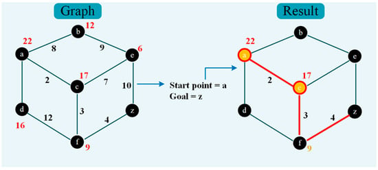
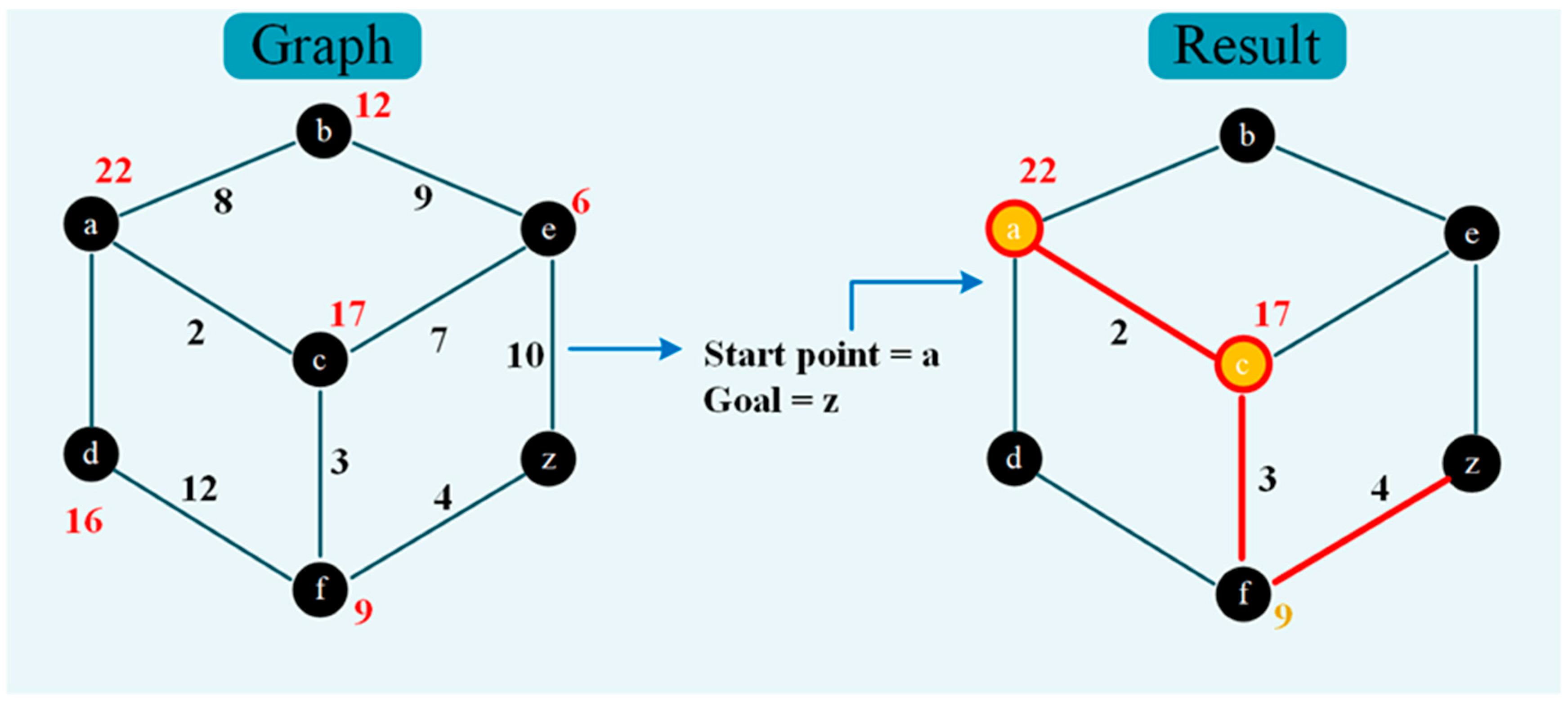
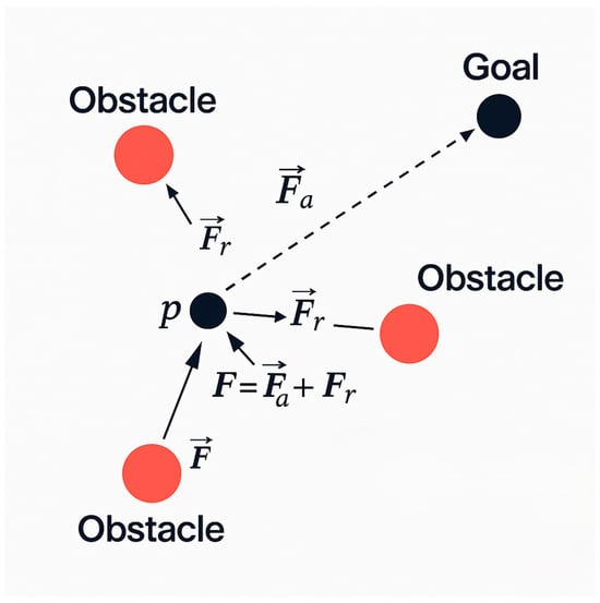
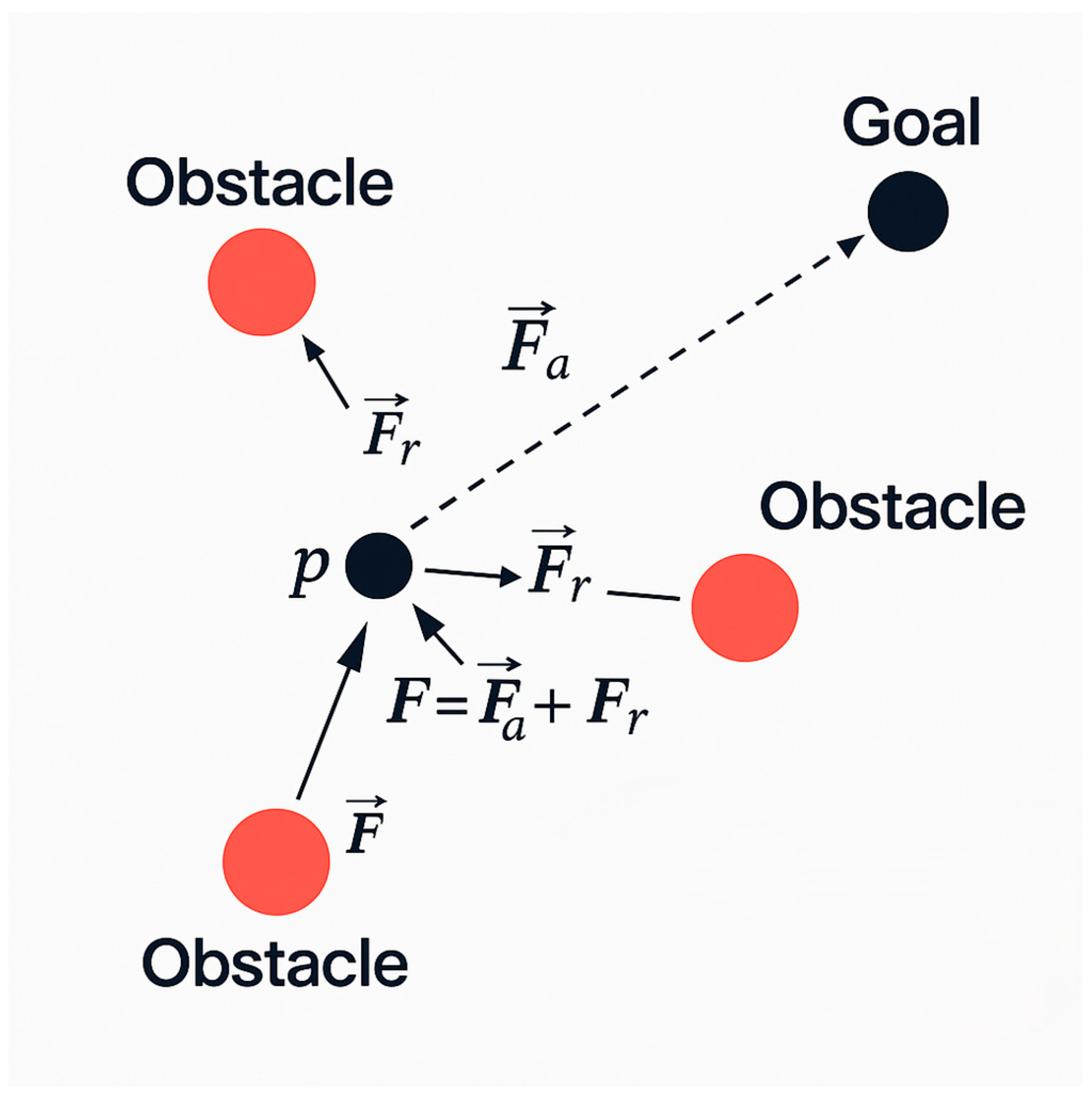
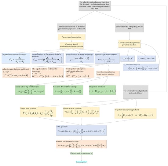
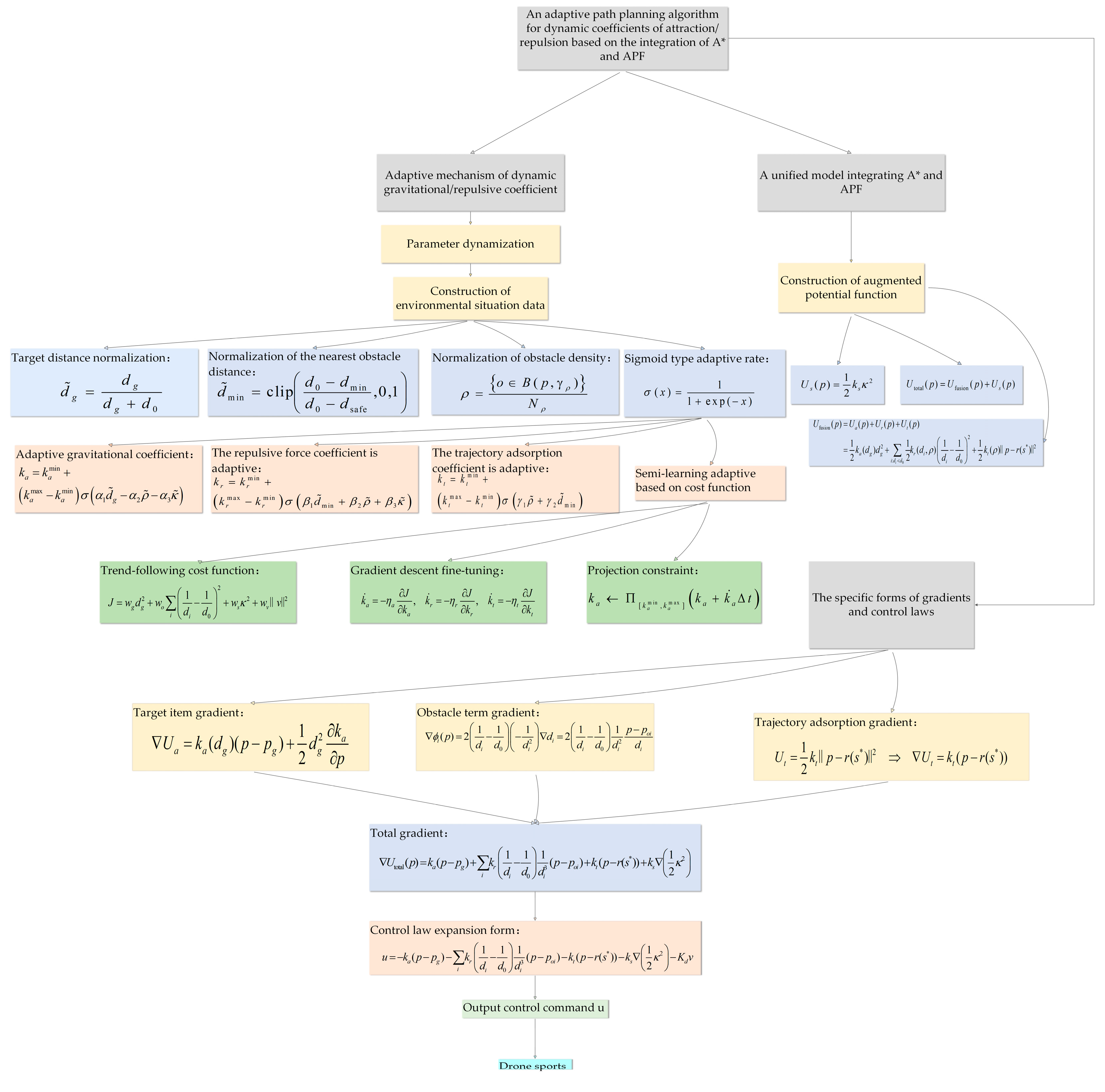
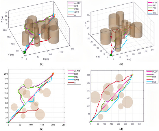
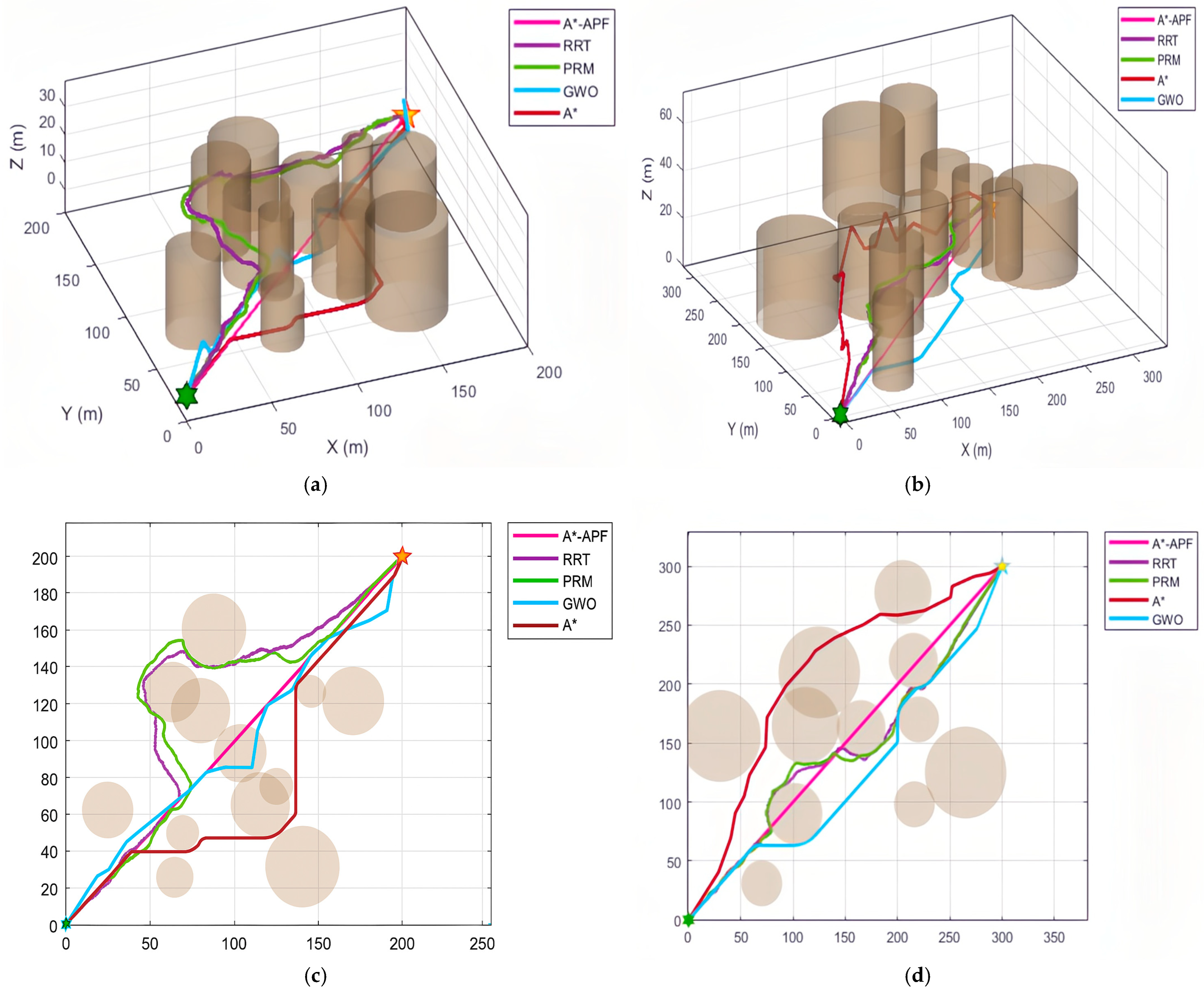
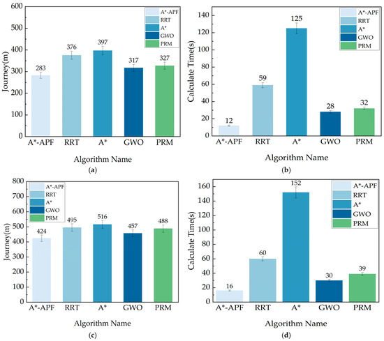
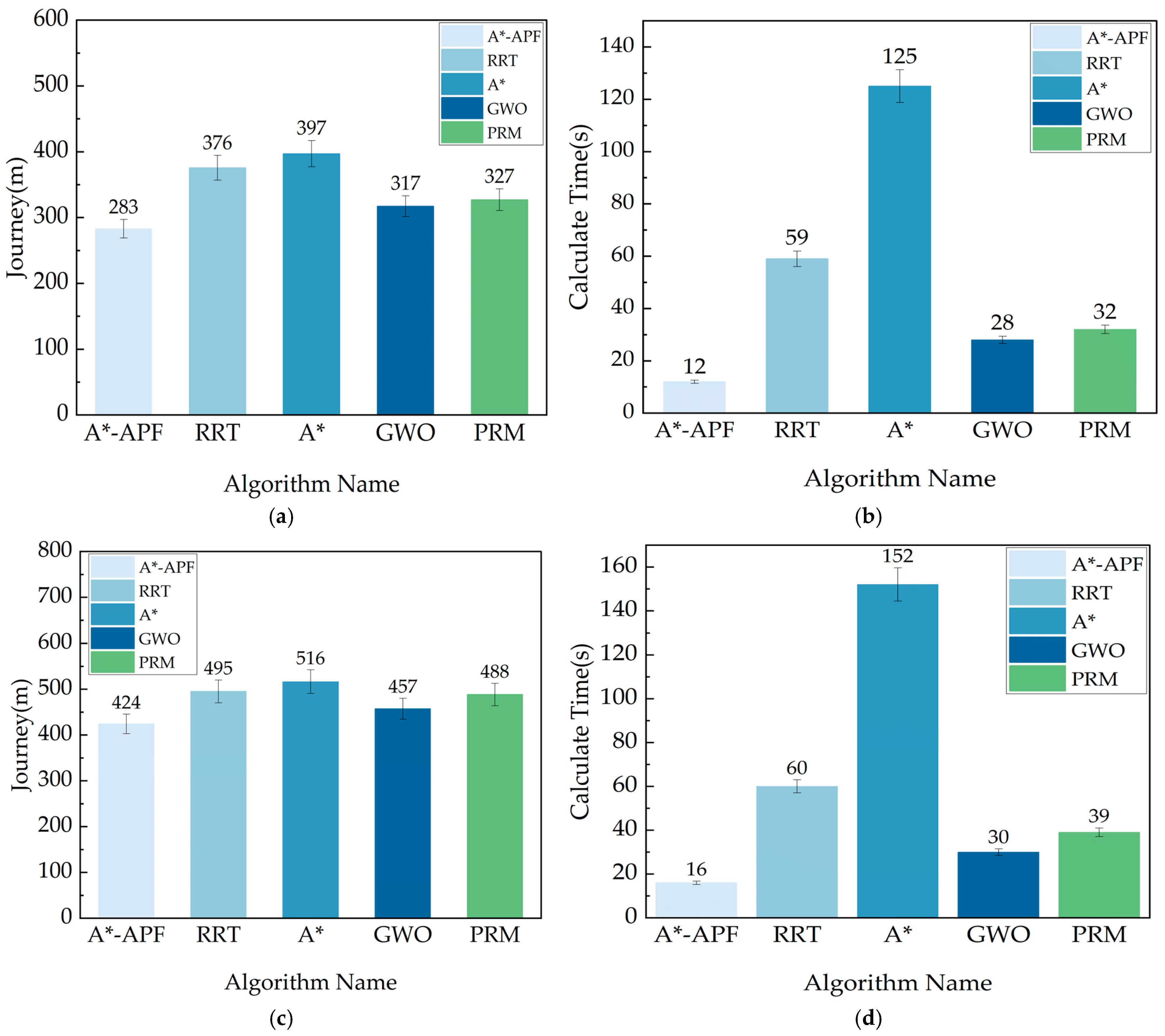
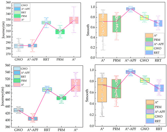
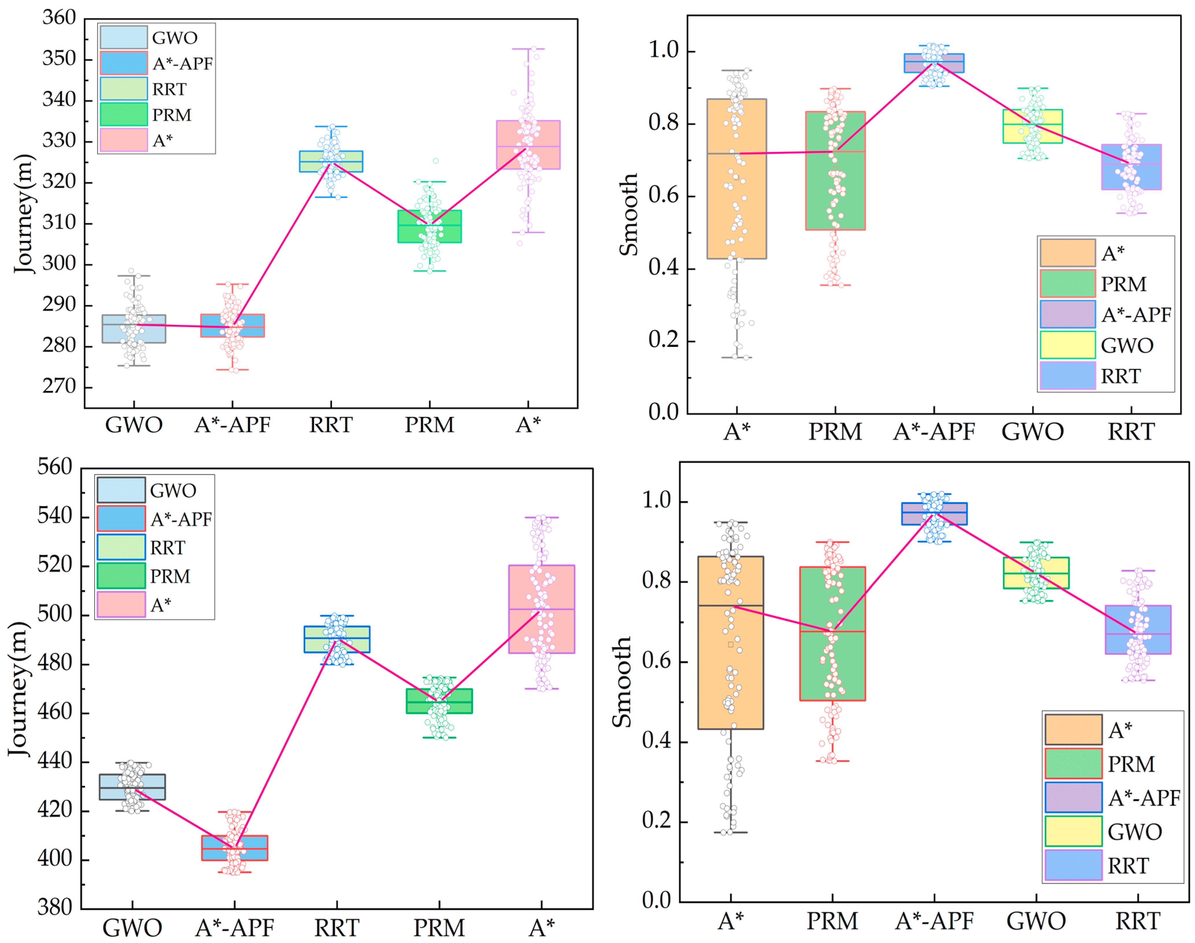
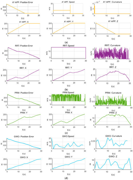
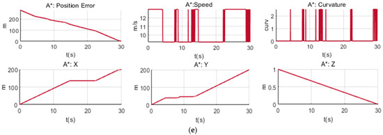
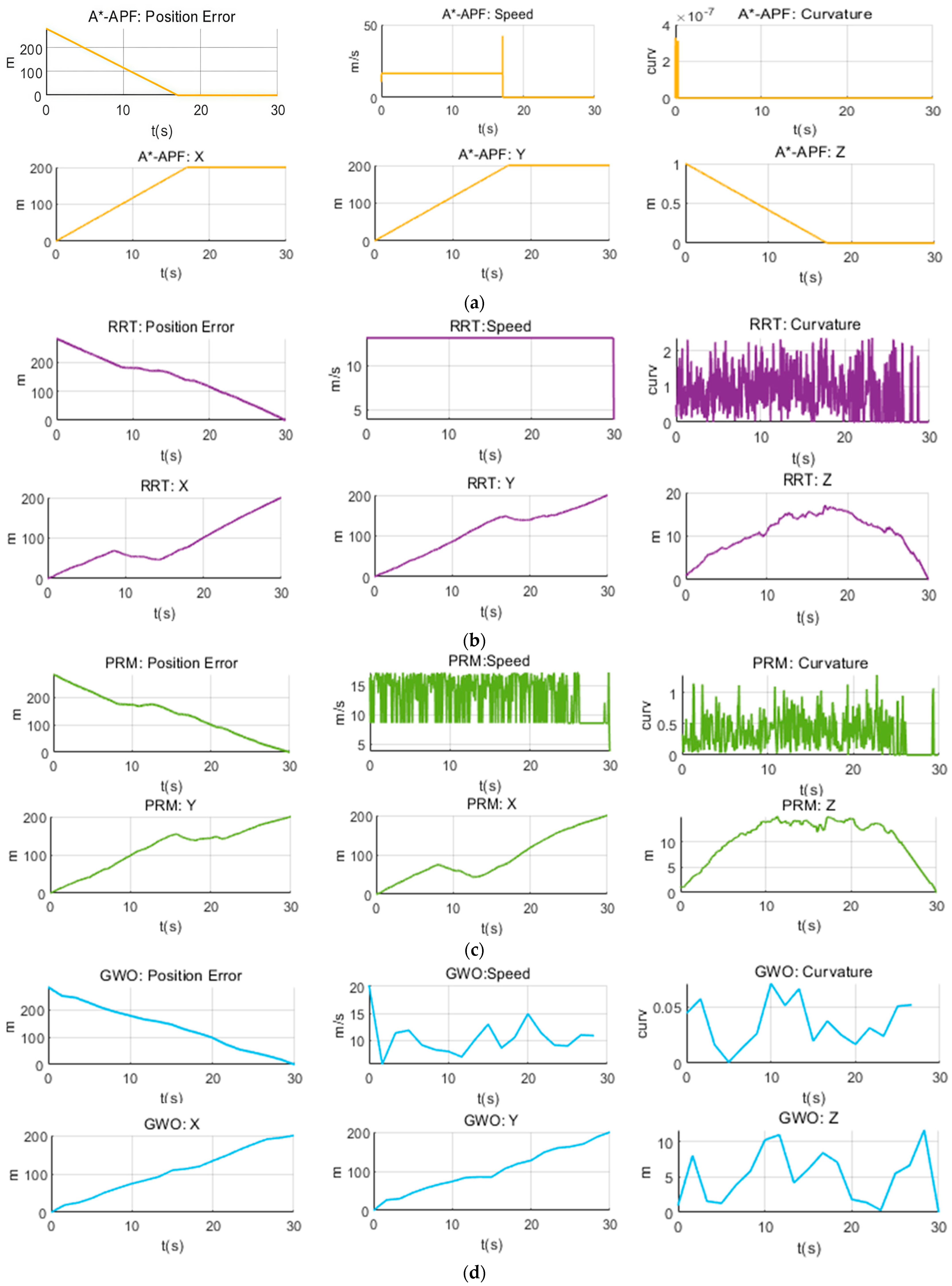
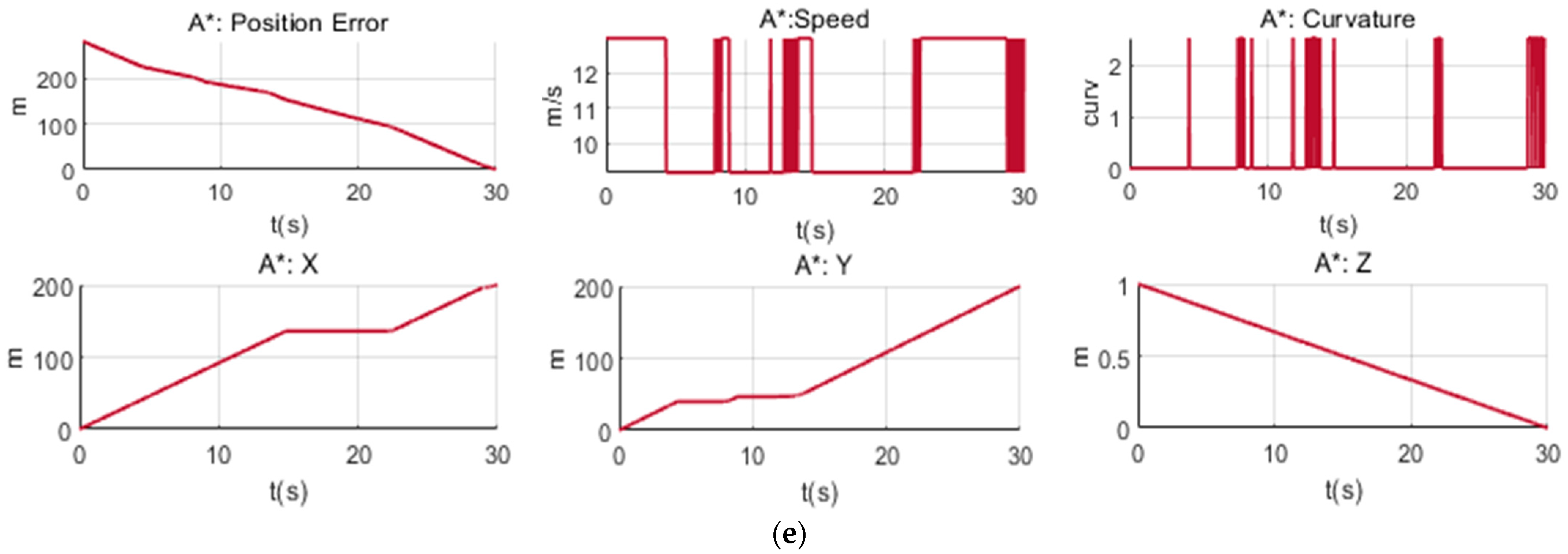
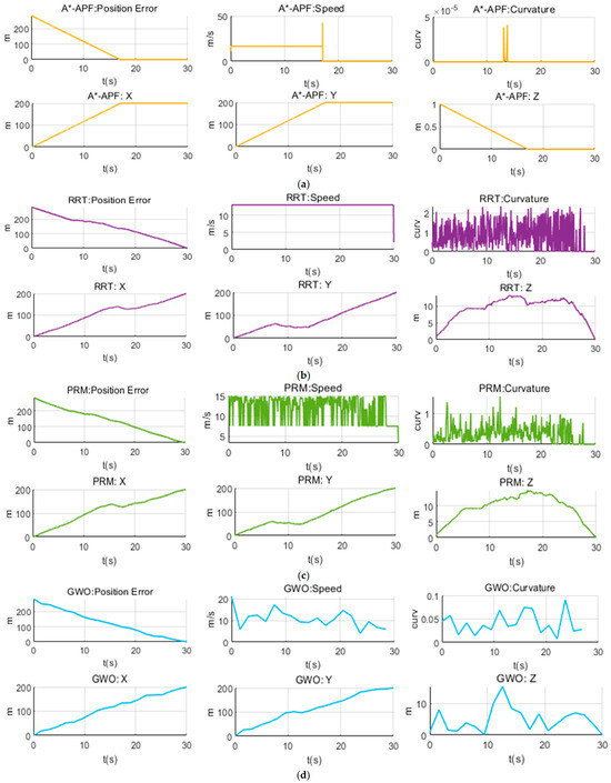
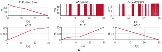
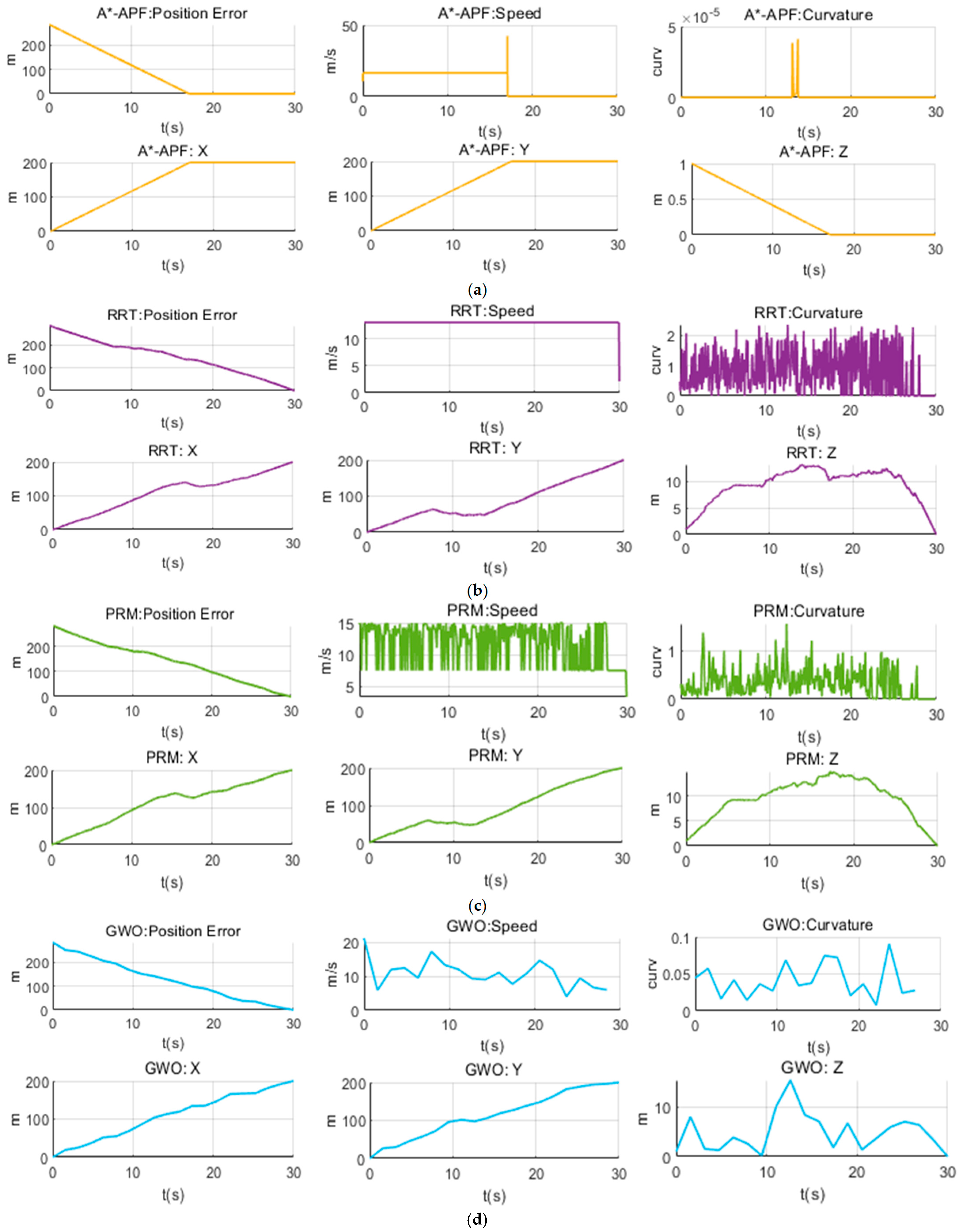
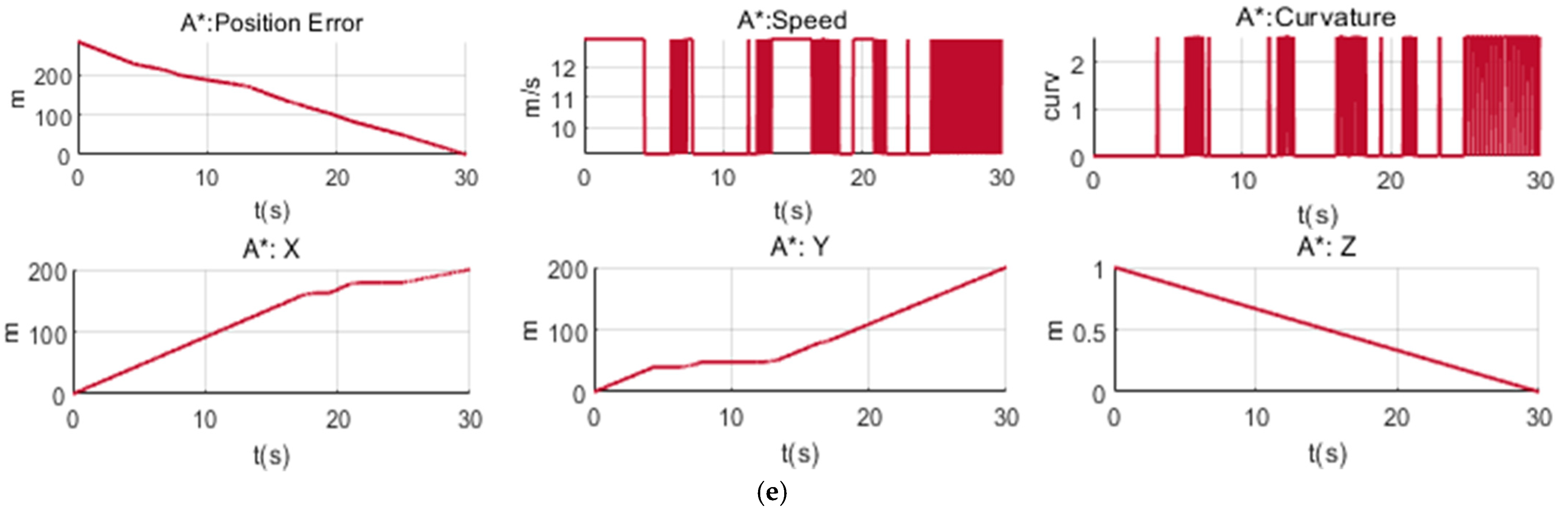
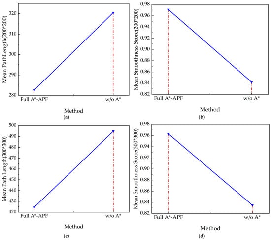
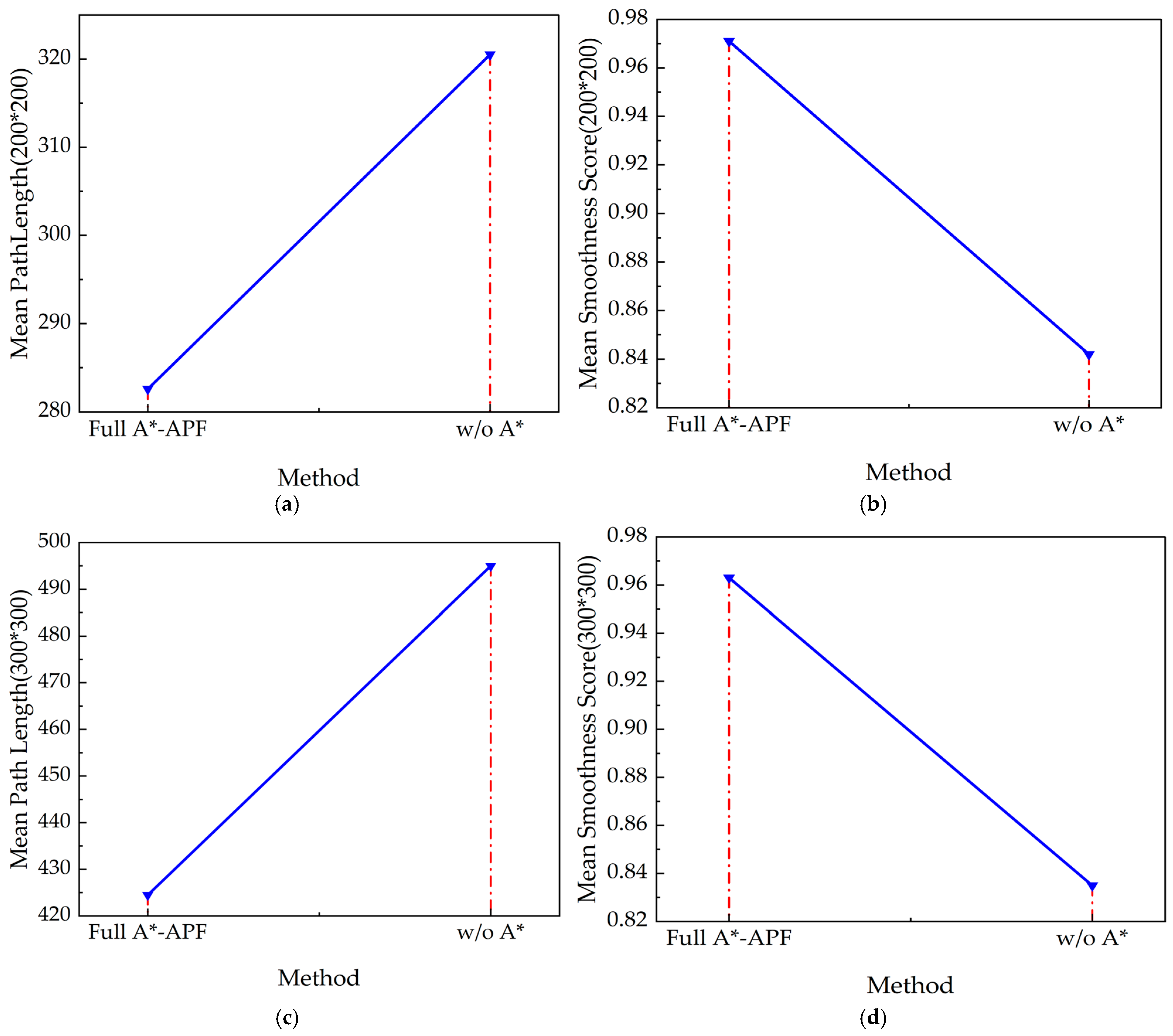
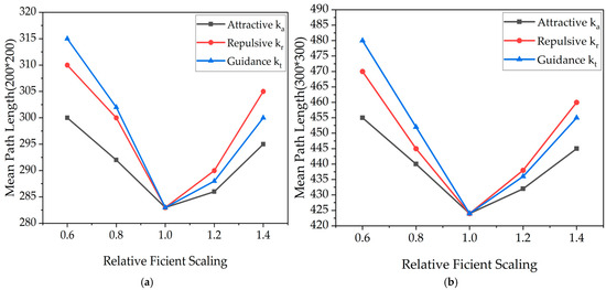
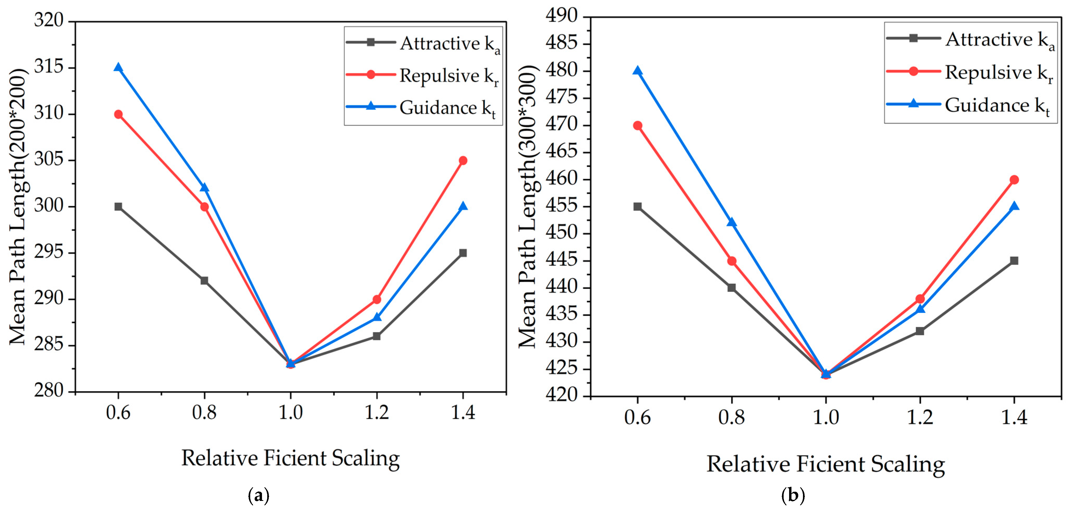
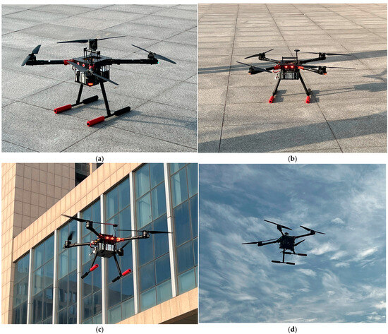
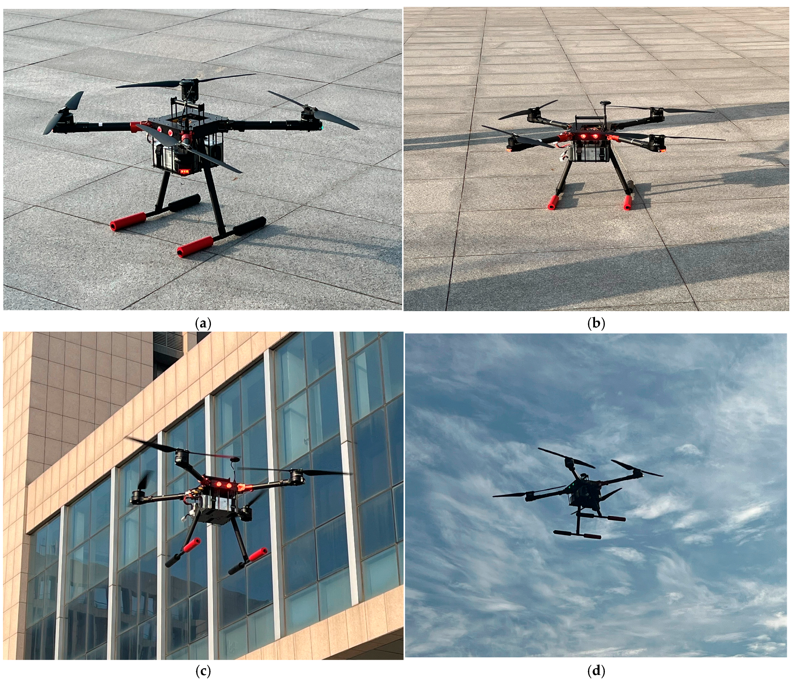
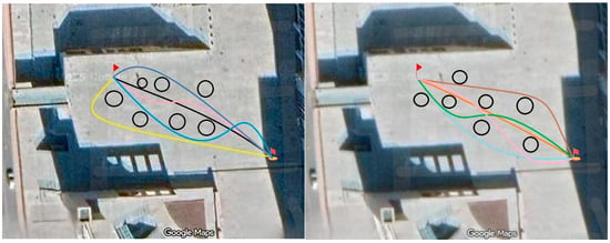
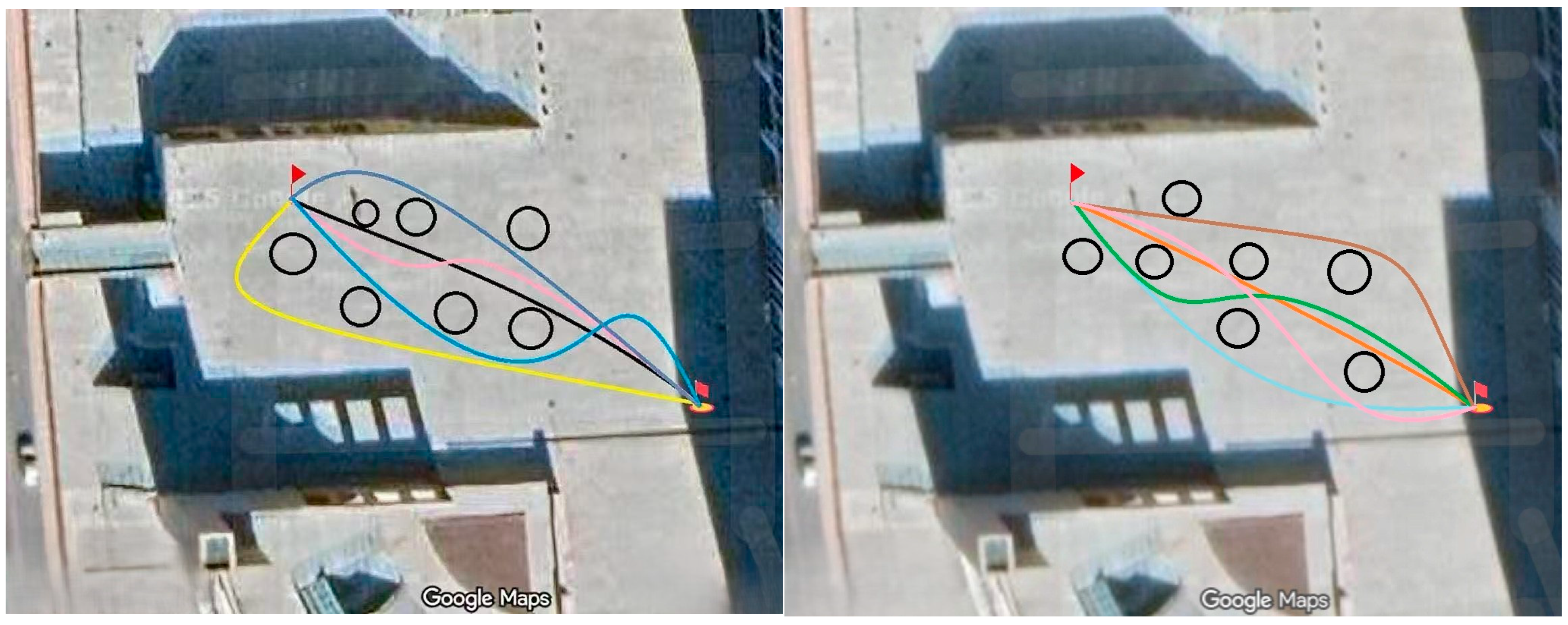
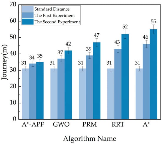
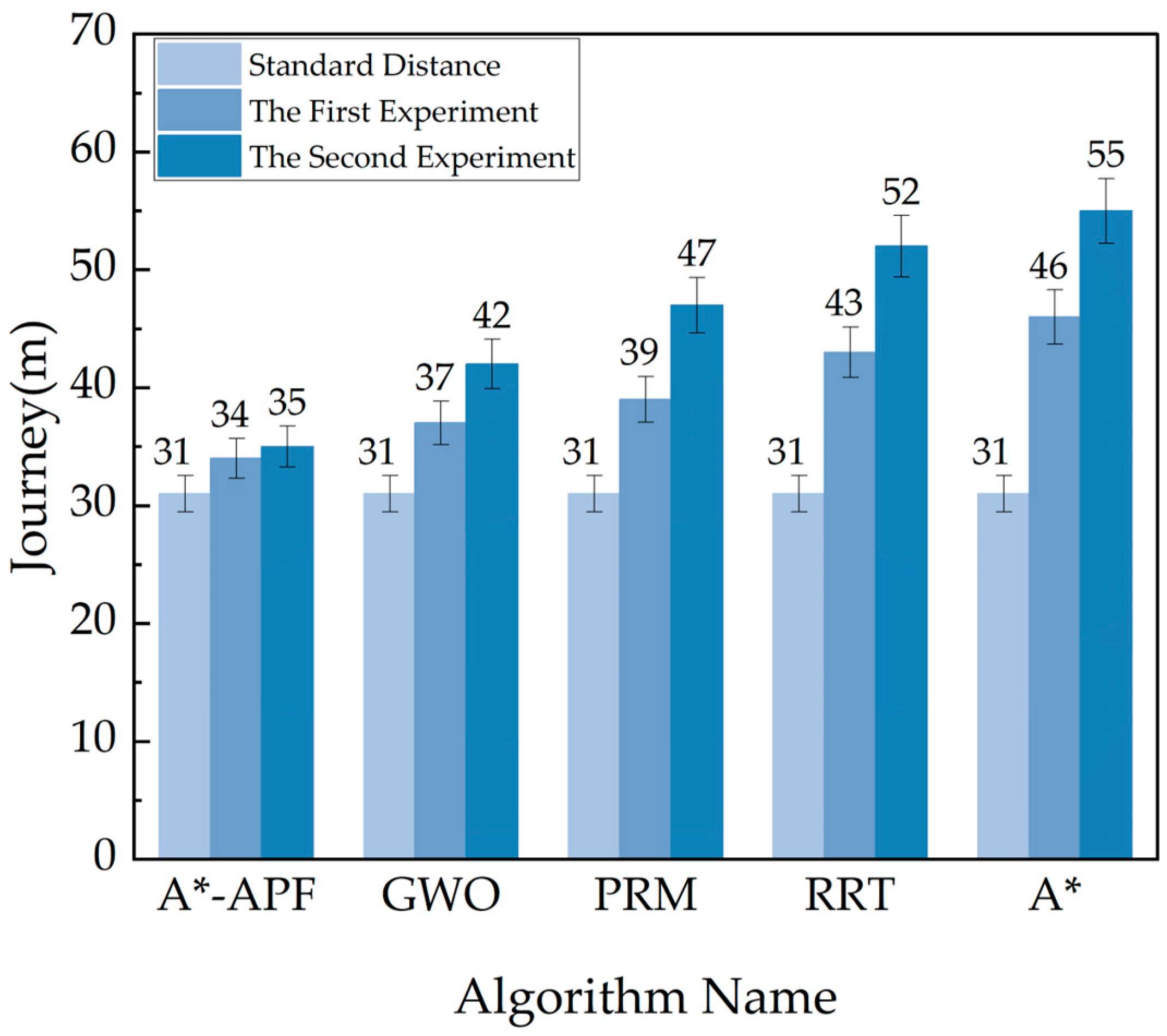

Disclaimer/Publisher’s Note: The statements, opinions and data contained in all publications are solely those of the individual author(s) and contributor(s) and not of MDPI and/or the editor(s). MDPI and/or the editor(s) disclaim responsibility for any injury to people or property resulting from any ideas, methods, instructions or products referred to in the content. |
© 2026 by the authors. Licensee MDPI, Basel, Switzerland. This article is an open access article distributed under the terms and conditions of the Creative Commons Attribution (CC BY) license.