Geometric Prior-Guided Multimodal Spatiotemporal Adaptive Motion Estimation for Monocular Vision-Based MAVs

Highlights

What are the main findings?

• This work proposesa Multimodal Decoupled Spatiotemporal Adaptive Network (MDSAN) that breaks the reliance of traditional motion estimation methods on the observer’s high-order motion, enabling high-precision 3D relative position and velocity estimation of dynamic MAVs, even in scenarios of low or no observability.
• This work develops two core modules (MSCN and STAS): MSCN achieves multimodal feature decoupling to avoid cross-modal contamination and suppress non-Gaussian noise, while STAS constructs a spatiotemporal collaborative modeling framework to reconstruct estimation constraints in low-observability scenarios.

What are the implications of the main findings?

• The main finding provides a new technical path for MAV swarm perception systems, balancing high precision, robustness, and cost-effectiveness by eliminating dependence on wireless communication and additional hardware.
• The main finding ddresses the unbalanced research status of MAV swarms (overemphasizing control while neglecting perception) and offers a practical solution to improve the reliability and cost-effectiveness of the swarm perception link.

Abstract

Estimating the relative position and velocity of micro aerial vehicles (MAVs) using visual signals is a critical issue in numerous tasks. However, traditional relative motion estimation algorithms suffer severely from non-Gaussian noise interference and have limited observability, making it difficult to meet the practical requirements of complex dynamic scenarios. To address this dilemma, this paper proposes a Multimodal Decoupled Spatiotemporal Adaptive Network (MDSAN). Designed for air-to-air scenarios, MDSAN achieves high-precision relative pose and velocity estimation of dynamic MAVs while overcoming the observability limitations of traditional algorithms. In detail, MDSAN is collaboratively composed of two core sub-modules: Modality-Specific Convolutional Normalization (MSCN) blocks and Spatiotemporal Adaptive State (STAS) blocks. Specifically, MSCN uses custom convolution kernels tailored to three modalities—visual, physical, and geometric—to separate their features. This prevents interference between modalities and reduces non-Gaussian noise. STAS, built on a state-space model, combines two key functions: it tracks long-term MAV motion trends over time and strengthens the synergy between different modal features across space. Adaptive weights balance these two functions, enabling stable estimation, even when traditional methods struggle with low observability. Furthermore, MDSAN adopts a full-vision multimodal fusion scheme, completely eliminating the dependence on wireless communication and reducing hardware costs. Extensive experimental results demonstrate that MDSAN achieves the best performance in all scenarios, significantly outperforming existing motion estimation algorithms. It provides a new technical path that balances high precision, high robustness, and cost-effectiveness for technologies such as MAV swarm perception.

1. Introduction

Micro aerial vehicle (MAV) swarm technology possesses significant research significance and practical application value in fields such as cooperative navigation, dynamic target tracking, swarm flight, autonomous search and rescue, and target encirclement (capture/protection) [1,2,3,4,5,6,7]. It has emerged as one of the core research directions in the field of robotics. In existing research, MAV swarm technologies predominantly focus on the control layer. Such studies generally design cooperative controllers under the assumption that each aircraft can obtain information on neighboring node status via wireless communication [3,8,9] while paying insufficient attention to the perception layer essential for stable swarm system operation. This reflects an imbalance in research priorities, emphasizing control over perception.

Notably, wireless communication-based methods for acquiring neighboring MAV information are prone to electromagnetic interference, transmission delay, and signal occlusion, leading to poor reliability. A few studies have adopted onboard visual sensors to detect neighboring MAVs for visual localization [10,11,12]. Full vision-based MAV visual localization methods can be completely independent of communication networks, realizing motion state estimation solely through visual information collected by cameras. Furthermore, they do not require additional deployment of sensing devices or the design of special detection algorithms, resulting in no extra hardware costs. This provides an ideal solution to resolve the contradiction between reliability and cost-effectiveness in MAV swarm perception. However, these methods still exhibit poor performance in terms of precision and robustness, failing to fully address the technical challenges.

In the development of all-visual relative position estimation, the bearing-only method [13] was the most widely used early approach. It uses target detection to obtain the target’s bounding box, then extracts the center pixel coordinates and combines them with a pinhole camera model to calculate the spatial bearing vector from the observer’s camera to the target. However, this algorithm imposes strict observational constraints. When using the bearing-only approachto estimate target motion, the observer must move in a lateral direction orthogonal to the target’s azimuth vector. These stringent motion limitations severely restrict its applicability in complex dynamic scenes. To overcome these observational limitations, Ning et al. proposed the bearing-angle method [14]. This approach enhances observability by incorporating the target bounding box’s angular information, effectively circumventing the bearing-only method’s reliance on additional lateral observer motion. However, the bearing-angle approach assumes angle measurement noise follows a Gaussian distribution. In real-world scenarios, bounding-box noise from deep learning object detectors exhibits a distinctly non-Gaussian distribution due to factors like target scale variations, partial occlusions, and illumination fluctuations. This Gaussian assumption severely underestimates the impact of extreme noise.

To address the noise-handling drawbacks of the bearing-angle method, we proposed the dynamic bearing-angle approach [15] in our previous work, which processes noise through a dual mechanism of weighted outlier suppression and dynamic noise intensity adaptation. Leveraging the Huber weight function of M-estimation, it assigns low weights to abnormal observations caused by issues such as instantaneous severe jitter of the bounding box, effectively suppressing impulsive, heavy-tailed, and other non-Gaussian noises. Meanwhile, it dynamically adjusts the noise covariance matrix via dynamic filtering in real time, accurately tracking changes in statistical noise characteristics, quickly adapting to target maneuvers, and shortening the convergence time. Additionally, it dynamically adjusts the smoothing coefficient based on the variance of the prior residual sequence, avoiding unstable filtering performance caused by fixed coefficients. This mechanism breaks the traditional fixed covariance assumption, resolves the problem of estimation performance deterioration induced by non-Gaussian and time-varying noises, and enhances robustness and accuracy in complex scenarios.

However, the aforementioned methods still suffer from critical drawbacks: the observability conditions are extremely stringent, as they generally rely on the strong assumption of a motion-order difference between the observer and the target [14] while failing to consider extreme cases of insufficient motion order. Although the motion-order advantage can theoretically guarantee observability, in practical scenarios, the observer often cannot achieve high-order motion due to path constraints, energy limitations, and other factors, directly leading to estimation divergence and tracking failure. More critically, existing methods are difficult to optimize through explicit modeling: explicit compensation for observability in low-order motion requires breaking of the boundaries of existing observability theory; the additional integration of devices such as LiDAR sensorsincreases costs, violating the core advantage of full-vision methods; and trading precision for stability fails to meet the high-precision requirements of MAV swarms. These contradictions make traditional algorithms unable to adapt to the practical demands of low cost and high reliability, highlighting an urgent need for new technical approaches to break through this predicament.

Therefore, to address the technical dilemma in current MAV motion estimation, where traditional methods suffer from limited observability due to their reliance on the observer’s high-order motion, this paper proposes an end-to-end motion estimation scheme based on multimodal decoupling and spatiotemporal adaptive modeling named the Multimodal Decoupled Spatiotemporal Adaptive Network (MDSAN). Without requiring the observer’s high-order motion, prior target-size information, or additional hardware deployment, it aims to solve the problem of high-precision 3D relative pose and velocity estimation for dynamic-attitude MAVs, providing a new path for improving the reliability and cost-effectiveness of MAV swarm perception. In detail, MDSAN achieves efficient motion estimation through two core modules. The MSCN block separates features from three modalities—visual, physical, and geometric. It uses unique convolution kernels and temporal optimization to keep each modality’s key dynamic information intact, reduce redundant data, and suppress non-Gaussian noise—all without letting one modality interfere with another.The STAS block realizes spatiotemporal collaborative modeling based on the State-Space Model (SSM) [16,17]. It first captures long-range inter-frame temporal dependencies to characterize MAV motion trends, then models cross-modal spatial correlations to enhance feature complementarity. Meanwhile, it introduces adaptive vision–geometry variance weights to further filter noise by judging cross-modal motion consistency.

By leveraging end-to-end temporal learning and multimodal collaborative optimization, MDSAN effectively integrates implicit visual information and geometric prior information, avoiding the stringent assumptions of traditional methods—such as the requirement for a motion-order difference between the observer and the target and the explicit construction of an attitude–size coupling model. Extensive experiments demonstrate that MDSAN achieves stable and high-precision MAV motion estimation, even in scenarios where the observer has no high-order motion or even no motion at all.

The contributions of this article are summarized as follows:

• We propose a Multimodal Decoupled Spatiotemporal Adaptive Network (MDSAN), which breaks the stringent reliance of traditional methods on the observer’s high-order motion. It fundamentally solves the problem of high-precision 3D relative pose and velocity estimation for dynamic-attitude MAVs, providing a new technical path for MAV swarm perception systems.
• We innovatively adopt a collaborative design of modality-specific decoupling and spatiotemporal adaptive modeling, combined with the end-to-end learning capability of deep learning. This eliminates the need for the explicit construction of attitude–size coupling models and static noise distribution models while suppressing non-Gaussian noise and retaining real MAV motion mutations through modality-specific processing.
• We address the unbalanced research status of MAV swarms (overemphasizing control while neglecting perception). The full-vision multimodal fusion scheme avoids reliance on wireless communication and additional hardware costs, and the cross-modal MSCN–STAS collaboration enhances perception robustness. This provides a practical and feasible solution to the problems of insufficient reliability and poor cost-effectiveness in the perception link of MAV swarms.

2. Related Works

The bearing-only approach [13] serves as the fundamental framework for visual target motion estimation, with its core lying in calculating the direction vector using the pixel coordinates of the target detection-box center and the pinhole camera model to achieve target position and velocity estimation. Early research focused on addressing filtering stability issues: Hoelzer et al. [18] proposed an improved polar coordinate method to separate observable and unobservable quantities, avoiding ill conditioning of the error covariance matrix; Aidala [19] revealed the divergence defect of the traditional Extended Kalman Filter (EKF) caused by the strong nonlinearity of bearing-only observations, promoting the development of alternative schemes such as pseudo-linear filtering and particle filtering. Notably, motion estimation and compensation have long been core techniques in video coding to remove temporal redundancy, with block-matching algorithms being a classic and efficient implementation [13], but such methods are designed for static frame compression and cannot adapt to the dynamic non-Gaussian noise and observability constraints in MAV motion estimation.

Lin et al. [20] further verified the balanced advantages of pseudo-measurement filtering between stability and real-time performance. Regarding observability, Fogel and Gavish [21] established the theory of Nth-order dynamic targets, clarifying the core constraint that when the target performs nth-order motion, the observer must execute $(n+1)$th-order motion with a lateral component. Subsequent studies, such as that by He et al. [22] optimizing trajectories based on the Fisher Information Matrix (FIM) and that by Li et al. [23] proposing 3D spiral guidance, all revolved around the satisfaction of this constraint. Multi-observer collaboration, such as in the spatiotemporal triangulation algorithm proposed by Zheng et al. [13], reduces the burden on a single observer but still requires some observers to achieve high-order motion, failing to break through the fundamental limitation.

To address the bearing-only method’s reliance on lateral motion, the bearing-angle approach [14] fuses the direction vector of the detection-box center with the opening angle derived from the box size. It incorporates the target’s physical size into the state vector and simplifies calculations via pseudo-linear Kalman filtering. Its key breakthrough lies in the relaxed observability conditions: without requiring the observer’s lateral motion, linear motion along the direction vector can still maintain observability through changes in the opening angle, resolving conflicts with task requirements. In single-view perception tasks, the combination of multimodal fusion with prior guidance has been proven effective in addressing scale ambiguity and lack of depth [24], providing valuable insights for breaking through the observability limitations in MAV motion estimation. In our previous work, we proposed the dynamic bearing-angle algorithm [15], which further optimizes robustness by introducing a dual mechanism of dynamic noise intensity adaptation and M-estimation-based outlier suppression. It dynamically adjusts the noise covariance and suppresses non-Gaussian noise through the Huber weight function, improving estimation accuracy in dynamic scenarios. However, it is essentially an optimization of the bearing-angle method’s performance and does not alter the core logic of observability.

From the perspective of observability, none of the three types of algorithms has broken through the limitation of motion-order difference: The bearing-only approach requires high-order motion with a lateral component; otherwise, observability degrades. Although the bearing-angle method relaxes the lateral constraint, it still demands the observer’s high-order motion to match the target dynamics. The dynamic bearing-angle approach only enhances dynamic robustness, without changing the underlying observability logic. This limitation constitutes a bottleneck in practical tasks: highly maneuverable targets require the observer to perform complex high-order motion, which not only increases energy consumption but may also conflict with the preset path. How to achieve stable estimation without relying on motion-order difference has become a core problem that urgently needs to be solved.

3. Method

Traditional motion estimation algorithms only use the 2D bounding boxes of MAVs in images as inputs for explicit modeling. However, explicit modeling suffers from observability limitations, making it constrained in practical scenarios. Fortunately, the visual features of the MAV to be estimated within the bounding box have not been effectively utilized. Therefore, this paper abandons the geometric calculation approach that relies on explicit motion-order constraints and shifts to data-driven implicit information fusion. This paper proposes a novel MAV motion estimation method named MDSAN. Addressing the observability constraints and non-Gaussian noise interference issues of traditional motion estimation methods, MDSAN fuses data-driven implicit information based on visual features with geometric prior information to achieve accurate end-to-end target position estimation, thereby avoiding the observability limitations of traditional methods.

3.1. Overview of the Multimodal Decoupling Spatiotemporal Adaptive Network

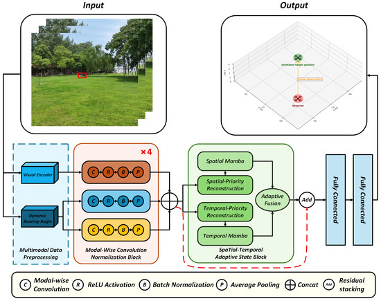
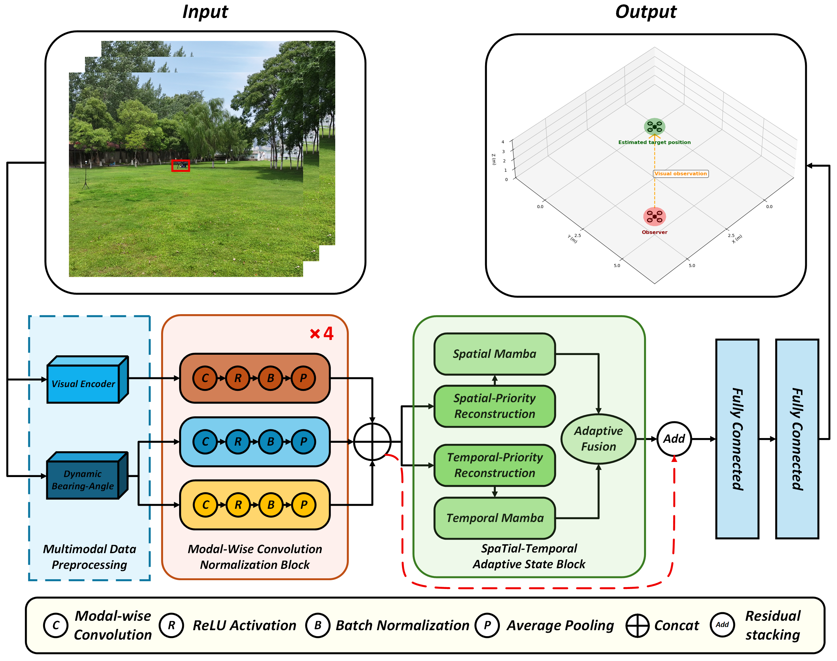
The overall structure of the proposed MDSAN is shown in Figure 1. We decompose $I_{ROI}$ into three modalities—visual, physical, and geometric—for separate processing. Specifically, regarding the visual features ($I_{ROI}$), we first resize $I_{ROI}$ to a uniform size of 64 × 64, then construct a visual encoder using MobileNetV2 [25] to extract deep semantic features ($X_{vis}$) of the MAV target. This process is mathematically expressed as follows:

$$X_{vis}=MobileNetV2\left(Resize(I_{ROI},64\times 64)\right),X_{vis}\in {\mathbb{R}}^{128}$$

(1)

Figure 1. The pipeline of the proposed the Multimodal Decoupling Spatiotemporal Adaptive Network.

We obtain physical and geometric modal characteristics through the dynamic bearing-angle algorithm [15]. The mathematical representation of this process is expressed as follows:

$$(X_{phy}^{init},X_{geo}^{init})=DBearingAngle(I_{BOX},P_{cam},R_c^w)$$

(2)

Among these, $P_{cam}$ is the internal reference matrix of the camera; $R_c^w$ is the rotation matrix from the camera frame to the world frame; $X_{geo}^{init}=[g_{\tau },{\theta }_{\tau }]\in {\mathbb{R}}^4$, where $g_{\tau }$ is the bearing vector and ${\theta }_{\tau }$ represents the azimuth angle; and $X_{phy}^{init}=[p_x,p_y,p_z,v_x,v_y,v_z]\in {\mathbb{R}}^6$, where p denotes the position and v represents the velocity. To address the limitations of low-dimensional features, we perform dimensionality elevation via a 1 × 1 convolutional layer with a learnable weight matrix and bias term, resulting in $X_{phy}\in {\mathbb{R}}^{32}$ and $X_{geo}\in {\mathbb{R}}^{16}$, which enrich the semantic expression of initial features.

Subsequently, we perform collaborative processing on the extracted multimodal temporal data through modal local feature decoupling and spatiotemporal correlation modeling. In this process, we propose two key modules: a Modality-Specific Convolutional Normalization (MSCN) block and a Spatiotemporal Adaptive State (STAS) block. The MSCN block is responsible for modality-specific processing of the three modalities (visual, physical, and geometric), avoiding cross-modal information interference and preserving the dynamic characteristics of each modality. Based on the State-Space Model (SSM), the STAS block first conducts temporal modeling to characterize the MAV motion trend, then performs spatial modeling to enhance feature collaboration and balances the spatiotemporal contributions through adaptive weights, ultimately breaking through the observability limitations of traditional methods. The overall mathematical relationship of this process can be expressed as follows:

$$F=STAS\left(Concat(MSCN\left(X_{vis}\right),MSCN\left(X_{phy}\right),MSCN\left(X_{geo}\right))\right)$$

(3)

where $Concat(·)$ represents feature concatenation, $MSCN(·)$ denotes the modality-specific normalization operation, and $STAS(·)$ stands for the spatiotemporal correlation modeling operation. This process not only ensures the purity of each modal feature by preventing cross-modal interference but also strengthens multimodal collaboration through spatiotemporal modeling, providing support for stable estimation in low-observability scenarios.

Finally, we map the intermediate feature (Y) to a 6-dimensional prediction through a fully connected network:

$$F{C}_1=SiLU\left(Linear(F,W_9,b_9)\right)$$

(4)

$$F{C}_2=SiLU\left(Linear(F{C}_1,W_{10},b_{10})\right)$$

(5)

$$Y=Linear(F{C}_2,W_{11},b_{11})\in {\mathbb{R}}^6$$

(6)

3.2. Modality-Specific Convolutional Normalization Block

Traditional multimodal temporal encoding often adopts the form of simple concatenation after unified convolution, which easily leads to cross-modal information contamination, loss of temporal fine-grained information, and poor modal adaptability. To address these issues, we designed the MSCN block. Through modality-specific convolution and temporal optimization, it achieves the decoupling, preservation, and enhancement of multimodal features, providing pure and highly distinguishable local features for the subsequent STAS block.

The modality-specificconvolution process is expressed as follows:

$$E_{conv}^m=Conv(X^m,W^m,b^m,K^m,stride=1)\in {\mathbb{R}}^{T\times D_m}$$

(7)

where $m\in \{vis,phy,geo\}$; $W^m$ denotes the modality-specific convolution kernel, $b^m$ is the modality-specific bias term, and $X^m$ represents the input modal feature. Targeting the temporal dynamic differences of different modalities, dedicated convolution kernels are designed for each of the three modalities. The kernel size is uniformly expressed as $k^m=2s^m+1$ through the kernel coefficient ($s^m$): the visual modality has strong locality of texture features, so $k^{vis}=3$; the physical modality requires medium-range dependence to capture motion trends, so $k^{phy}=5$; and the correlation between the direction angle and opening angle of the geometric modality needs long-range temporal capture, so $k^{geo}=7$. The convolution operation only acts on the current modal feature and does not share parameters across modalities, fundamentally avoiding cross-modal information contamination.

In the temporal optimization stage, ReLU is first applied to retain fine-grained features; then, batch normalization is used to stabilize the training distribution. The formula is expressed as follows:

$$E_{BN}^m=BN\left(ReLU\left(E_{conv}^m\right)\right)$$

(8)

Subsequently, average pooling with a stride of 2 is adopted to reduce the temporal length from T to $L=T/2$, reducing redundancy while retaining temporal mean features:

$$E_m=E_{pool}^m=AvgPoo{l}_2(E_{BN}^m,stride=2)\in {\mathbb{R}}^{L\times D_m}$$

(9)

Finally, the outputs of the three modalities are concatenated along the feature dimension to form the final output of MSCN: $E=[E_{vis},E_{phy},E_{geo}]\in {\mathbb{R}}^{L\times 176}$.

3.3. Spatiotemporal Adaptive State Block

The STAS block is constructed based on the SSM. Through spatiotemporal modeling and adaptive fusion, it efficiently captures multimodal long-range spatiotemporal dependencies and cross-modal correlations while dynamically balancing the contributions of each modality. It fundamentally avoids the reliance of traditional methods on the observer’s high-order motion and adapts to complex dynamic scenarios of MAVs. First, discretization adaptation of the SSM is performed. Since MAV motion data are frame-level temporally discrete signals, the Zero-Order Hold (ZOH) method is used to discretize the continuous SSM. The discretization formulas are expressed as follows:

$$\overline{A}=exp(\Delta A)$$

(10)

$$\overline{B}={(\Delta A)}^{-1}·\left(exp\right(\Delta A-I\left)\right)·\Delta B$$

(11)

where $\Delta =1/f$ is the sampling interval, $A\in {\mathbb{R}}^{64\times 64}$ and $B\in {\mathbb{R}}^{64\times 1}$ are the continuous SSM parameters, and $exp(·)$ denotes the exponential matrix operation. To enhance the adaptability of the SSM to dynamic MAV changes, input-dependent parameters are introduced, enabling $\overline{A}$, $\overline{B}$, and $\Delta$ to be adjusted with input features:

$${\overline{A}}_t={\Delta }_t\otimes A_{param}$$

(12)

$${\overline{B}}_t={\Delta }_t\otimes Linea{r}_B\left(E_t\right)$$

(13)

$${\Delta }_t=Softplus(Linea{r}_{\Delta }\left(E_t\right)+{\theta }_s)$$

(14)

$${\overline{C}}_t=Linea{r}_C\left(E_t\right)$$

(15)

where $A_{param}$ adopts the HIPPO matrix to enhance the ability to capture long-range temporal dependencies; $Linea{r}_B$, $Linea{r}_{\Delta }$, and $Linea{r}_C$ are modality-shared linear projection layers; ${\theta }_s$ is a learnable bias term; ⊗ represents the element-wise product operation; and $Softplus\left(z\right)=log(1+exp(z\left)\right)$ ensures ${\Delta }_t>0$.

In the temporal modeling stage, Temporal Mamba is responsible for characterizing long-range temporal dependencies: the output (E) of MSCN is rearranged to prioritize the temporal dimension as $E^{Temp}=rearrange(E;L\times 176\to 176\times L)\in {\mathbb{R}}^{176\times L}$, and the multimodal temporal dynamics are modeled through Temporal SSM:

$$F_{Temp,t}={\overline{C}}_{Temp,t}·S_{Temp,t}={\overline{C}}_{Temp,t}·({\overline{A}}_{Temp,t}·S_{Temp,t-1}+{\overline{B}}_{Temp,t}·E_{Temp,t})$$

(16)

where ${\overline{A}}_{Temp,t}$, ${\overline{B}}_{Temp,t}$, and ${\overline{C}}_{Temp,t}$ are Temporal SSM parameters and $S_{Temp,t}$ is the hidden state vector.

In the spatial modeling stage, Spatial Mamba is responsible for capturing cross-modal correlations: E is rearranged to explicitly distinguish the modal dimension as $E^{Spat}=split(E;dim=1,split=[128,32,16])\in {\mathbb{R}}^{L\times 176}$, and the multimodal complementary correlations are modeled through Spatial SSM to output spatial features:

$$F_{Spat,t}={\overline{C}}_{Spat,t}·S_{Spat,t}={\overline{C}}_{Spat,t}·({\overline{A}}_{Spat,t}·S_{Spat,t-1}+{\overline{B}}_{Spat,t}·E_{Spat,t})$$

(17)

Finally, adaptive fusion is performed: the global variance of visual features (${\sigma }_{vis}$) and the global variance of geometric features (${\sigma }_{geo}$) are combined to dynamically adjust weights, balancing the contributions of temporal and spatial features. The formulas are expressed as follows:

$$w_{Temp,t}={\displaystyle \frac{{\sigma }_{vis}}{{\sigma }_{vis}+{\sigma }_{geo}}}$$

(18)

$$w_{Spat,t}=1-w_{Temp,t}$$

(19)

Meanwhile, the output (E) of MSCN is superimposed as a residual connection to avoid gradient vanishing, and the final output of STAS is obtained:

$$F=w_{Temp,t}·F_{Temp}+w_{Spat,t}·F_{Spat}+E$$

(20)

This feature not only contains long-range spatiotemporal dependencies but also integrates multimodal collaborative information, providing strong support for subsequent pose regression.

3.4. Loss-Function Design

To ensure the regression accuracy of position and velocity in a single frame, enhance the motion continuity within the temporal window, and avoid non-physical jumps in prediction results, the following loss function is designed:

$$L_{total}=L_{reg}+\lambda ·L_{TempSmooth}$$

(21)

The core regression loss ($L_{reg}$) adopts Mean Squared Error (MSE) to optimize the prediction errors of position and velocity, adapting to the requirements of continuous value regression. It is mathematically expressed as follows:

$$L_{reg}=\alpha ·L_{pos-MSE}+\left(1-\alpha \right)·L_{vel-MSE}$$

(22)

Specifically, let the predicted position and velocity of the model be ${\widehat{p}}_k$ and ${\widehat{v}}_k$ and the corresponding ground truths be $p_{k,gt}$ and $v_{k,gt}$. Then, the position loss is $L_{pos-MSE}={\displaystyle \frac{1}{3}}{\sum }_{k=x,y,z}{({\widehat{p}}_k-p_{k,gt})}^2$, and the velocity loss is $L_{vel-MSE}={\displaystyle \frac{1}{3}}{\sum }_{k=x,y,z}{({\widehat{v}}_k-v_{k,gt})}^2$.

To characterize the motion continuity of MAVs and constrain the variation deviation of predicted values between adjacent frames in the temporal window, a temporal smoothness loss ($L_{TempSmooth}$) is constructed. It is mathematically expressed as follows:

$$L_{TempSmooth}={\displaystyle \frac{1}{6(L-1)}}\sum _{t=1}^{L-1}(\Vert {\widehat{p}}_{k,t+1}-{\widehat{p}}_{k,t}{\Vert }^2+\Vert {\widehat{v}}_{k,t+1}-{\widehat{v}}_{k,t}{\Vert }^2)$$

(23)

Through experimental testing, the training parameters are set as $\alpha =0.7$, $\lambda =0.1$, and $L=5$.

4. Real-World Experimental Results

4.1. Experimental Settings

4.1.1. Implementation Details

All experiments reported in this paper are completed in a unified hardware and software environment. We use the PyTorch 1.7.1 framework to implement the model proposed in this paper and use two NVIDIA GeForce RTX 3090 graphics cards for model training and testing. The training process adopts the AdamW optimizer with an initial learning rate $1\times {10}^{-4}$, weight decay of $1\times {10}^{-4}$, and batch size of 16. The total number of training epochs is 200, and the learning rate is reduced to $1\times {10}^{-4}$ at epoch = 50.

4.1.2. Metrics

We directly use the distance error and velocity error to evaluate motion estimation accuracy, with smaller distance and velocity errors indicating better performance.

The distance error is calculated using the Euclidean distance, reflecting the accuracy of the spatial position estimation of the target within a single frame and mathematically expressed as follows:

$$PE=\sqrt{{({\widehat{p}}_x-p_{x,gt})}^2+{({\widehat{p}}_y-p_{y,gt})}^2+{({\widehat{p}}_z-p_{z,gt})}^2}$$

(24)

The velocity error refers to the deviation between the estimated velocity and the true velocity and is also calculated using the Euclidean distance, reflecting the accuracy of the motion velocity estimation of the target. It is mathematically expressed as follows:

$$VE=\sqrt{{({\widehat{v}}_x-v_{x,gt})}^2+{({\widehat{v}}_y-v_{y,gt})}^2+{({\widehat{v}}_z-v_{z,gt})}^2}$$

(25)

In quantitative analysis, we adopt the Average Distance Error (ADE), Average Velocity Error (AVE), and Root Mean Square Error of Distance (D-RMSE) to evaluate motion estimation accuracy, with smaller ADE, AVE, and D-RMSE values indicating better performance [15].

4.1.3. Baselines

We verified the effectiveness of our method by comparing it with the state-of-the-art bearing-angle, dynamic bearing-angle, and classic bearing-only methods. For a fair comparison, we conducted simulations using publicly available code and parameter settings adjusted specifically for the task addressed in this paper.

4.1.4. Datasets

To verify the performance of the proposed visual target motion estimation algorithm in real-world scenarios, this study adopts the MAV6D dataset and MS-MAV-ViME as experimental benchmarks, utilizing their image sequences and corresponding annotation information for validation.

The MAV6D dataset is constructed via an indoor automated data collection platform, consisting of three core components: the VICON motion capture system, a monocular camera, and the target MAV. It achieves strict spatiotemporal alignment of data through a timestamp synchronization mechanism. The VICON system outputs a high-precision 6D pose ground truth of the MAV at a sampling frequency of 100 Hz, while the monocular camera captures 640 × 480 pixel images at 20 Hz and provides complete intrinsic and extrinsic parameters. The target MAV flies within a restricted area of 1–6 m, with retroreflective markers attached to its body to ensure the accuracy of ground-truth capture. The dataset contains 57,075 annotated images and 129 video sequences, covering multiple maneuver modes, multi-view variations, and scenarios with different distances.

Additionally, the current MAV motion estimation field lacks real-world air-to-air motion estimation datasets. To further verify the generalization and robustness of the algorithm, we additionally constructed the MS-MAV-ViME dataset for comparative validation, with detailed descriptions provided in Section 4.2.

4.2. Multi-Scenario MAV Visual Motion Estimation Dataset

Currently, the MAV motion estimation field generally lacks real-world air-to-air motion estimation data. Most existing studies rely on simulated environments, in which it is difficult to reproduce complex factors such as non-Gaussian noise and dynamic interactions in real scenarios. This makes it impossible to effectively verify the actual performance of algorithms in low-observability scenarios. To address this, we specifically construct the multi-scenario MAV visual motion estimation dataset (MS-MAV-ViME), whose core goal is to provide real and comprehensive measured data support for the proposed MDSAN method, and systematically verify the algorithm’s robustness and high-precision estimation capability in different dynamic interaction scenarios.

4.2.1. Hardware Platform Configuration

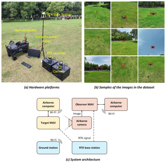
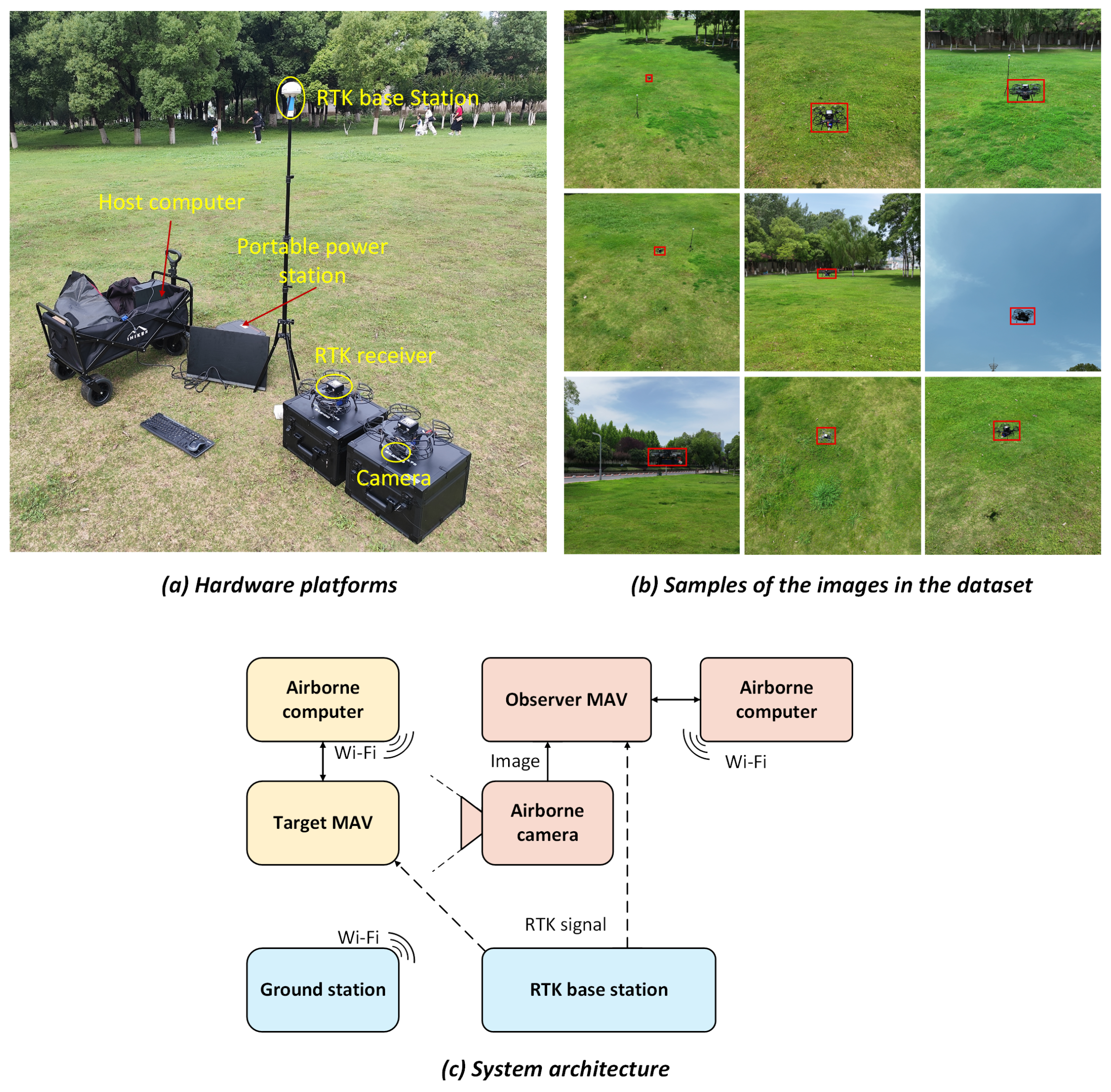
Data collection is based on two flight platforms developed with OWL mini3 quadrotor UAVs (Figure 2a). Each platform is equipped with an RTK GPS module, a binocular vision module integrated with an IMU (achieving precise self-localization through the fused Visual–Inertial Odometry (VIO) algorithm), a 2-axis gimbal stabilizer, and an RGB gimbal camera. Meanwhile, the true velocity of the UAV is calculated in real time from the fused data of the RTK module and IMU synchronously collected and stored by the onboard VISBOT platform with a sampling frequency consistent with that of the RTK positioning data (10 Hz), ensuring spatiotemporal correlation between velocity and position data.

Figure 2. The setup of the MAV-to-MAV motion estimation experiment.

In terms of control and storage, the onboard flight controlleradopts the VISBOT onboard platform (equipped with an 8-core CPU and a 6TOPS NPU) and the Enzo Pro 4th-generation flight controller. Remote connection is realized via a 5G-band Wi-Fi module, and the collected data, such as images and position and velocity information, are stored on the onboard computer in real time. Furthermore, the centimeter-level position reference provided by the RTK module, the enhanced accuracy in dynamic velocity measurement provided by the IMU, and the effective cancellation of flight jitter through the gimbal stabilizer further ensure the stability of image collection, laying a solid foundation for subsequent multimodal feature extraction and motion estimation. The key parameter specifications of each hardware platform are shown in Table 1, and the structure of the hardware perception and communication system is illustrated in Figure 2c.

Table 1. Key specifications of the outdoor hardware system.

Component	Parameter	Value	Unit
OWL 3	Diagonal size	200	mm
	Max speed	20	m/s
	Max flight time	26	min
	Total mass	675	g
RTK	Accuracy	1	cm
	Max frequency	10	Hz
Camera	Resolution	1920×1080	pixel
	Max frequency	30	Hz

4.2.2. Data Collection

During the data collection phase, the target MAV and the observer MAV flew along specified trajectories at set speeds according to predefined control commands, covering core scenarios such as chasing, circling, and static observation, with viewing angles including three typical types: top-down, bottom-up, and front-facing. Meanwhile, the gimbal camera of the observer MAV adjusted its attitude in real time using an automatic control algorithm to ensure the target MAV remained within the camera’s field of view throughout the process, avoiding data invalidation caused by target loss.

A total of 21 valid data sequences were obtained. The video data was stored in MP4 format with an original frame rate of 30 Hz and a resolution of $1920\times 1080$ pixels. Each individual sequence in the collected data had a duration of 20–120 s, resulting in a total of 46,624 frames for the dataset, with an overall duration of approximately 25.9 min. The corresponding RTK position data and IMU-fused velocity data were both sampled at 10 Hz, and the true velocity values were recorded and stored synchronously with the position data, fully preserving the spatiotemporal motion states of the target and observer MAVs. The motion scenarios captured in the dataset included six sub-scenarios—circular motion, linear following, linear following after oblique cut-in, static observation, target-forbidden observer reciprocating motion, and random maneuvering—comprehensively covering complex dynamic interaction scenarios.

During data collection, the camera, RTK module, and IMU all collected data based on GPS timestamps to ensure the temporal unity of multi-source data. Specifically, each frame of the video recorded by the camera was embedded with a GPS timestamp with an accuracy of $\pm 1$ ms. The RTK position data and IMU-fused velocity data were synchronously associated with GPS timestamps during recording, and the timestamps of the velocity data and position data were strictly aligned (deviation $\le 1$ ms), effectively guaranteeing the time traceability and spatiotemporal consistency of the original data. Additionally, when storing data, the onboard computer established index associations between image frames, position data, and velocity data based on GPS timestamps. All images and flight data were stored on the onboard computer, and subsequent annotation and performance comparison were completed through offline processing. Examples of measured data images are shown in Figure 2b.

4.2.3. Data Processing

During the data processing phase, the original 30 Hz video data is first clipped into individual frames and downsampled to 10 Hz to ensure a sampling frequency matching with the 10 Hz RTK position data and IMU velocity data. Subsequently, a target detection and tracking algorithm constructed based on PRL-Track and YOLOv11s [26] is adopted to automatically extract the 2D bounding boxes (ROI regions) of the target MAV from each frame, laying the foundation for subsequent multimodal feature extraction. Furthermore, based on GPS timestamps, frame-by-frame alignment of the 10 Hz image frames, RTK position data, and IMU velocity data is achieved through nearest-neighbor matching. The image frame closest to the timestamp of the position–velocity data is selected as a valid frame to ensure the spatiotemporal synchronization of visual features, position ground truth, and velocity ground truth in single-frame data. All image data are uniformly resized to $640\times 480$ pixels to adapt to the input requirements of the model’s visual encoder.

After alignment, the temporal deviation between the image frames, RTK position data, and IMU velocity data is ≤3 ms, among which the internal synchronization deviation between velocity data and position data is ≤1 ms. This precision fully meets the stringent requirements of spatiotemporal synchronization for offline performance comparison and real-time motion estimation, ensuring that the temporal error between multi-source data will not affect the validity of algorithm evaluation.

All data sequences are divided as follows to ensure the objectivity of performance evaluation: 14 sequences for model training, 2 sequences for validation and parameter tuning, and 5 sequences for independent testing (the test data did not participate in the model training process).

4.2.4. MS-MAV-ViME Typical Test Scenarios

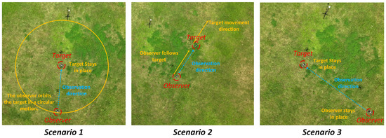
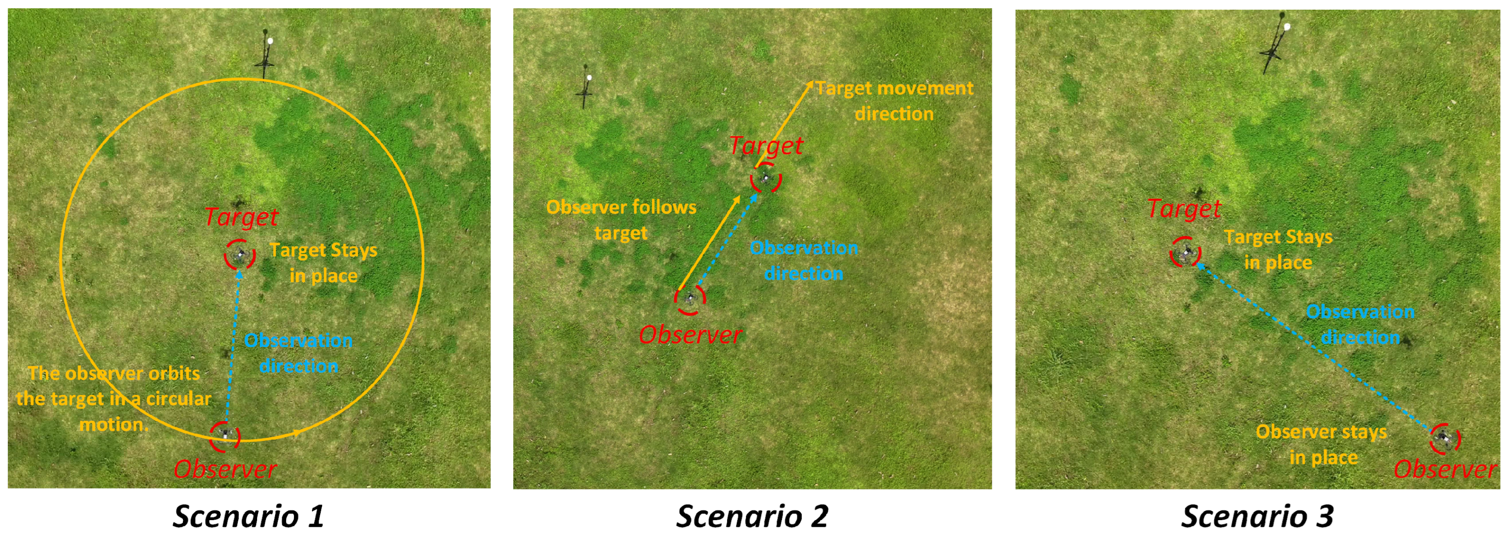
We present test results from three typical motion scenarios, where the data was not used for training. Detailed experimental settings are presented as follows (Figure 3):

Figure 3. Overview of experimental scenario setup.

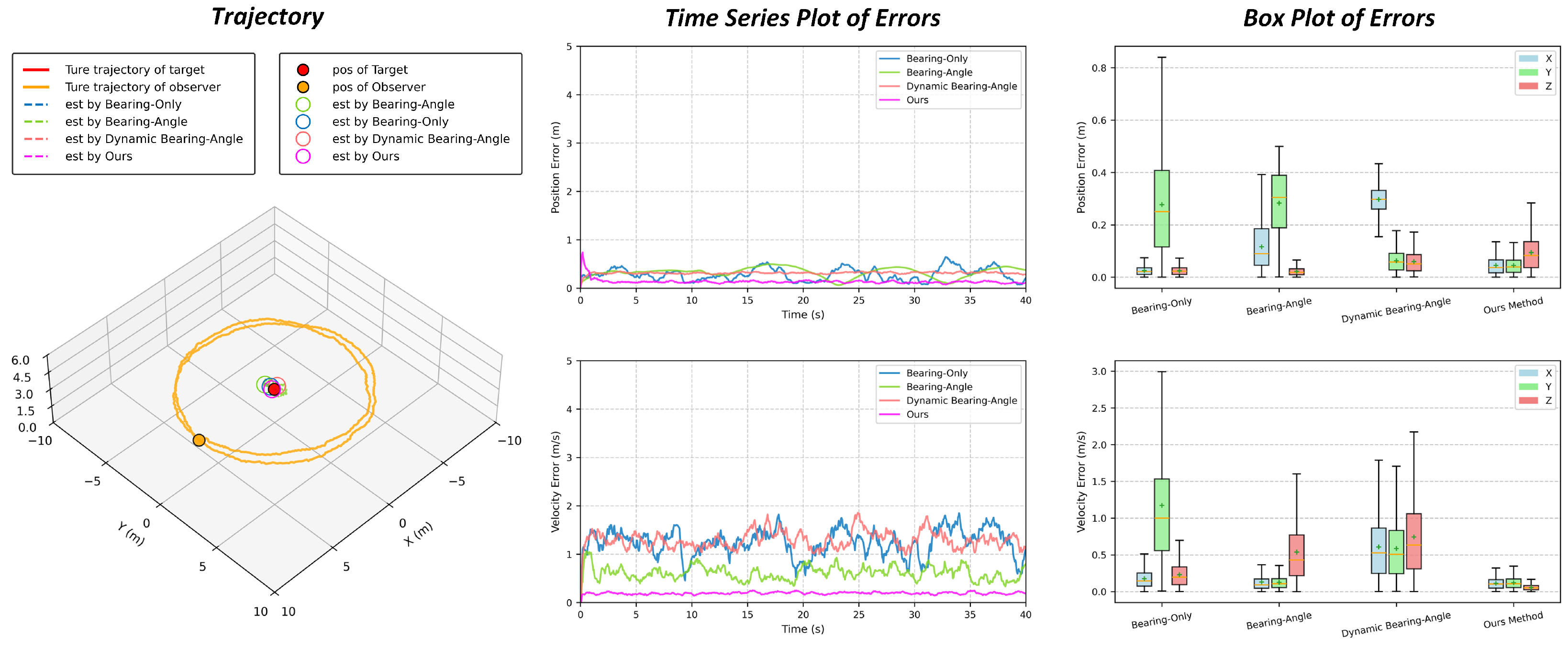
• Scenario 1: Circular Motion Around the Target (Strong Traditional Observability): In the initial stage, both the observer and the target UAVs activate all deployed algorithms on the ground. After the ground control station sends the take-off command, the target UAV moves to a height of 2 m and hovers, while the observer UAV moves to a height of 3 m and flies along a circular trajectory with the target as the center and a radius of 6 m (angular velocity: 0.5 rad/s). During the movement, the target UAV remains approximately stationary, and the observer UAV’s circular motion provides sufficient lateral movement, ensuring the estimation algorithm obtains adequate relative motion parameters as inputs. Meanwhile, the observer UAV exhibits high-order motion relative to the target. Although the measured values fluctuate slightly due to measurement noise interference, the sufficient lateral relative motion and the presence of high-order motion in this scenario result in strong observability.
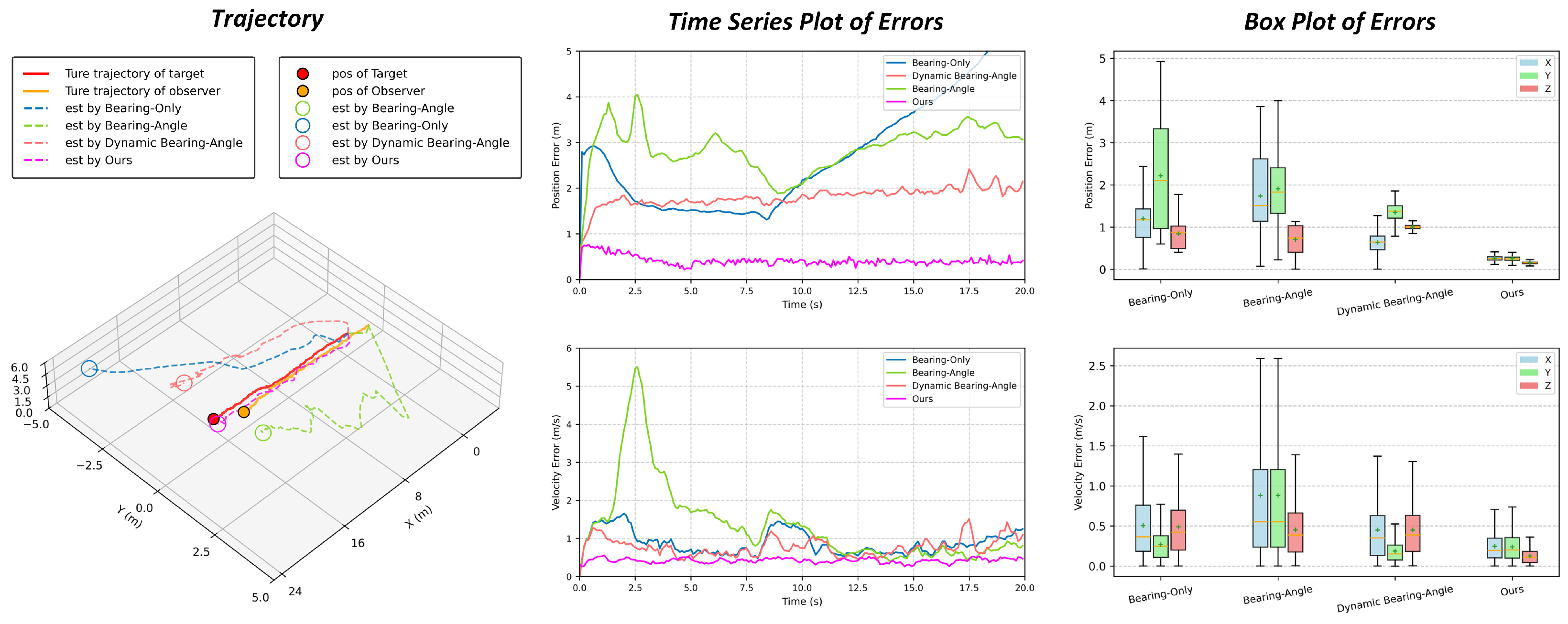
• Scenario 2: Linear Motion Following the Target (Weak Traditional Observability): In the initial stage, both the observer and the target UAVs activate all deployed algorithms on the ground. After the ground control station sends the take-off command, the target UAV moves to a height of 2 m, and the observer UAV hovers at a height of 3 m, 2.2 m directly behind the target. The target UAV adopts a motion pattern of “uniform linear motion-braking and hovering-uniform linear motion”: it moves at a constant speed of 1.2 m/s from 0 to 8 s, brakes and remains stationary (velocity = 0) from 8 to 10 s, then moves at a constant speed of 1.2 m/s again from 10 to 20 s. The observer UAV’s motion strategy is outlined as follows: it hovers in a stationary position for observation from 0 to 1.2 s, then follows the target at a speed of 1.2 m/s after 1.2 s, brakes and hovers in a stationary position for observation from 8 to 10 s, and finally moves at a constant speed of 1.2 m/s to follow the target from 10 to 20 s. During the entire movement process, there is no lateral motion (no orthogonal component of the direction vector) between the observer and the target in any phase. Additionally, a relative motion-order difference exists only in an extremely short time period (e.g., the observer is initially stationary, and the observer lags in braking). Therefore, the scenario exhibits almost no observability.
• Scenario 3: Stationary Observer Monitoring the Target (No Traditional Observability): In the initial stage, both the observer and the target UAVs activate all deployed algorithms on the ground. After the ground control station sends the take-off command, the target UAV moves to a height of 3 m, and the observer UAV hovers at the same height of 3 m (6 m away from the target) and continuously monitors the target for 60 s. In this scenario, there is no significant relative motion between the target and the observer in any direction of the 3D space; only bounding-box observation noise associated with the detection algorithm disturbs the measurements. Moreover, there is no high-order motion (complete immobility), resulting in no observability in this scenario.

4.3. Experimental Results on MAV6D

We conducted tests on the MAV6D dataset, where four typical frame intervals were selected. The Average Distance Error (ADE) and Distance Root Mean Square Error (D-RMSE) were adopted to evaluate the accuracy of target position estimation, and the results are shown in Table 2.

Table 2. Performance comparison results on the MAV6D dataset.

Method	Frame 0~20		Frame 21~40		Frame 41~100		Frame After 100
	ADE	D-RMSE	ADE	D-RMSE	ADE	D-RMSE	ADE	D-RMSE
Bearing Only	2.7629	3.6741	2.8384	3.2344	1.9722	2.0180	2.4395	2.8725
Baseline Angle	2.1502	2.2752	1.4824	1.4825	1.1017	1.1349	1.3070	1.5678
Dynamic Bearing Angle	1.2404	1.5808	0.4986	0.7352	0.4237	0.4814	0.3631	0.3660
MDSAN	0.2135	0.2742	0.1518	0.1926	0.1207	0.1536	0.1103	0.1329

Experimental results show that in the comparative tests on the MAV6D dataset, the target position estimation accuracy of MDSAN across all frame intervals is significantly superior to that of traditional methods. In the initial phase, it responds quickly and effectively avoids observability constraints, enabling faster convergence and stable estimation errors compared with traditional methods. In high-speed maneuvering scenarios, MDSAN effectively suppresses noise interference through the collaborative encoding of multimodal features, continuously maintaining the error convergence state. During long-term tracking, the spatiotemporal modeling mechanism of MDSAN can effectively capture long-term motion trends and suppress error accumulation, consistently maintaining the position prediction error at a low level, while other traditional methods exhibit significant error fluctuations. The experimental results fully verify the strong robustness against noise and long-term estimation stability of MDSAN in indoor scenarios.

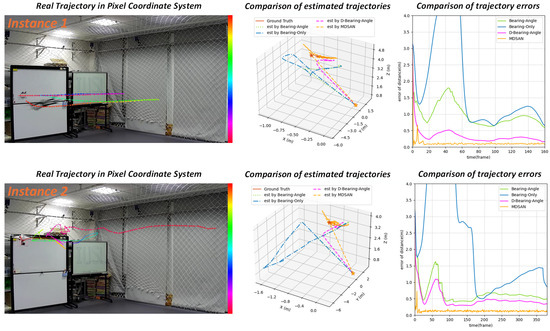
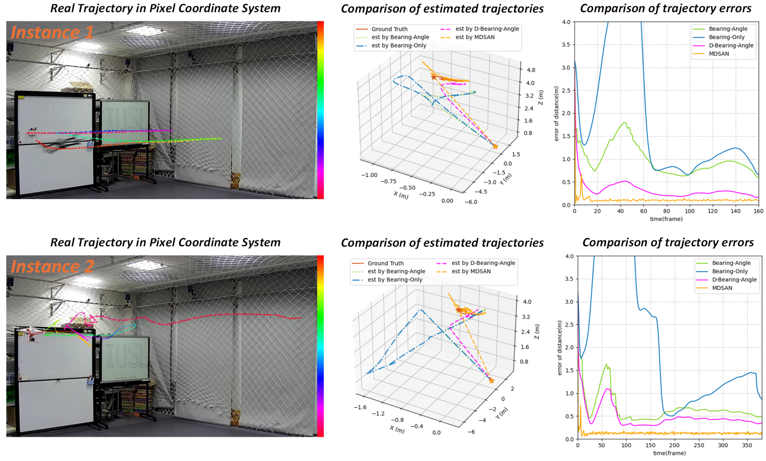
To intuitively compare the specific differences among various methods, we visualized two typical examples in detail, as shown in Figure 4. According to the results presented in the figure, both types of maneuver scenarios satisfy the strong observability conditions of sufficient lateral motion and significant motion order difference. None of the methods experienced fundamental failure, but there were significant performance differences. The bearing-only method performs the worst, with large error peaks and the most severe fluctuations, and the error further amplifies in the later stage of rapid lateral maneuvering. This is because it only relies on pure bearing-angle information, lacks depth constraints, cannot decouple the coupling relationship between distance and position, and is highly sensitive to measurement noise and maneuver changes. The bearing-angle approach introduces target opening-angle constraints, increasing the observation dimension, and its error level is between those of the bearing-only and D-bearing-angle methods. However, assuming a Gaussian noise distribution and without optimization for non-Gaussian noise in real scenarios, it still exhibits obvious error accumulation. Through a robust dual mechanism, the D-bearing-angle approach effectively suppresses part of the non-Gaussian noise interference, and its error performance is slightly better than that of the bearing-angle method, but it fails to break through the core limitations of traditional methods.

Figure 4. Test results in two instances are illustrated in the figures. The first column shows the ground-truth trajectory of the MAV in the pixel coordinate system, where gradient-colored lines with arrows indicate the positions of the MAV at different time steps. The second column presents a comparison of the estimated trajectories of various methods. The third column displays the curve of trajectory error varying with the number of frames.The five-pointed stars in the figure indicate the initialization positions for each algorithm.

In contrast, the estimated trajectory of MDSAN considerably overlaps with the ground-truth trajectory under both maneuver modes, and the error is always maintained in a stable range with low fluctuations. It rapidly converges after only minor jitter during the algorithm initialization phase, fully demonstrating its adaptability to different high-maneuver scenarios.

4.4. Experimental Results on MS-MAV-ViME

To comprehensively evaluate the performance of the proposed method, we conducted experiments in the three typical scenarios mentioned above, comparing it with mainstream methods including the bearing-only, bearing-angle, and dynamic bearing-angle methods. The experimental results are analyzed with respect to three dimensions: trajectory estimation accuracy, stability of error time series, and error boxplots.

• Scenario 1 Test Results

In this scenario, there exists a significant relative motion-order difference, sufficient lateral motion, and continuous dynamic changes in the azimuth angle during observation. These conditions provide adequate calculation constraints for all methods; thus, all methods can effectively estimate the target position, with only differences in precision and stability rather than fundamental failure.

As shown in Figure 5, the trajectory of the proposed method almost completely overlaps with the ground truth, achieving the highest position and velocity estimation accuracy, along with with the smallest and most stable errors and no obvious fluctuations. This advantage stems from its in-depth observability optimization through threefold innovative fusion while satisfying basic observability conditions: the dynamic bearing-angle guidance mechanism enhances robustness against dynamic noise, effectively offsetting minor disturbances during measurement; temporal modeling can accurately capture motion trends, smooth instantaneous measurement errors, and further improve estimation stability; and visual feature encoding expands the observable dimension, successfully decoupling the coupling relationship between position and velocity. Compared with traditional methods, it adds an additional spatial constraint, thereby achieving optimal precision.

Figure 5. Results of experiments in circular motion around the target scenarios.

The bearing-angle method can complete basic position estimation but exhibits obvious deviations. The core reason is its single measurement modality—relying solely on bounding-box information, without additional temporal or visual feature supplementation. It has poor resistance to measurement noise and no dynamic noise adaptation, so minor fluctuations in circular motion are directly reflected in the estimation results. The dynamic bearing-angle approach outperforms the bearing-angle method, with relatively smaller deviations, as it adds a dynamic noise adaptation mechanism based on the bearing-angle method, which can partially offset measurement noise and trajectory fluctuations in circular motion. Although the bearing-only method can effectively estimate the target position, it has the largest offset, the most obvious fluctuations, and the worst accuracy. Its fundamental limitation lies in its sole reliance on direction vectors for calculation, its lacks of range and bearing information, and its inability to decouple distance and position relationships (e.g., targets at different distances with the same azimuth angle cannot be distinguished by a single direction vector and can only be indirectly calculated based on azimuth-angle changes caused by lateral motion, resulting in inherently limited precision). Additionally, it is sensitive to measurement noise and has no robustness optimization mechanism, so minor disturbances in circular motion are directly amplified into position offsets.

• Scenario 2 Test Results

In this scenario, the observer follows the target from the rear, maintaining forward-facing camera alignment with the target in front, with no lateral motion and an approximately zero relative motion-order difference. As shown in Figure 6, the bearing-only approach exhibits severe trajectory drift and extremely high error peaks, and it directly diverges during the phase when the target and observer are relatively stationary, completely failing to achieve stable estimation. This is because its observability is completely lost: it lacks the rigid constraint of lateral motion, suffers from motion-order mismatch, and has no azimuth-angle changes during the stable phase. A single direction vector cannot calculate the target state, and without any optimization mechanism, it immediately loses the basis for calculation once the azimuth angle stabilizes, leading to complete estimation failure.

Figure 6. Results of experiments in Linear motion following target scenarios.

Although the bearing-angle method relaxes the lateral motion constraint, it still lacks a relative motion-order difference, and its measurement modalities (only bearing and angle) cannot cope with the time-varying characteristics of linear maneuvers. This method has insufficient precision and poor stability, with obvious fluctuations in its estimated trajectory, which may be caused by its inability to handle large observation noise during air-to-air relative motion. The dynamic bearing-angle approach shows significant trajectory deviations, frequent error oscillations, and a divergence trend in the later observation stage. Although its performance is better than that of the bearing-angle method, it fails to solve the fundamental observability problem. After the azimuth angle stabilizes in the stable phase, lacking additional constraints from temporal and visual features, dynamic noise adaptation alone cannot maintain observation effectiveness, resulting in a divergence trend. In contrast, the trajectory of the proposed method closely matches the ground truth, with position and velocity errors remaining stable at a low level, without drift or lag. The core lies in its reconstruction of observability through threefold fusion: dynamic bearing-angle guidance can match the time-varying noise of linear maneuvers in real time, avoiding errors caused by model mismatch; temporal modeling can capture long-term motion trends, making up for the lack of short-term constraints due to unchanged azimuth angles and smoothing fluctuations; and visual feature encoding expands the spatial observable dimension and decouples the coupling relationship between distance and size. Without relying on lateral motion or azimuth-angle changes, the dual constraints of time and space form redundant guarantees, enabling it to maintain high observability throughout the process.

• Scenario 3 Test Results

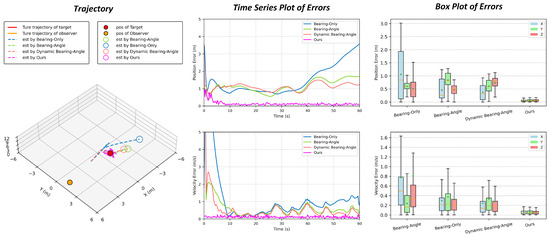
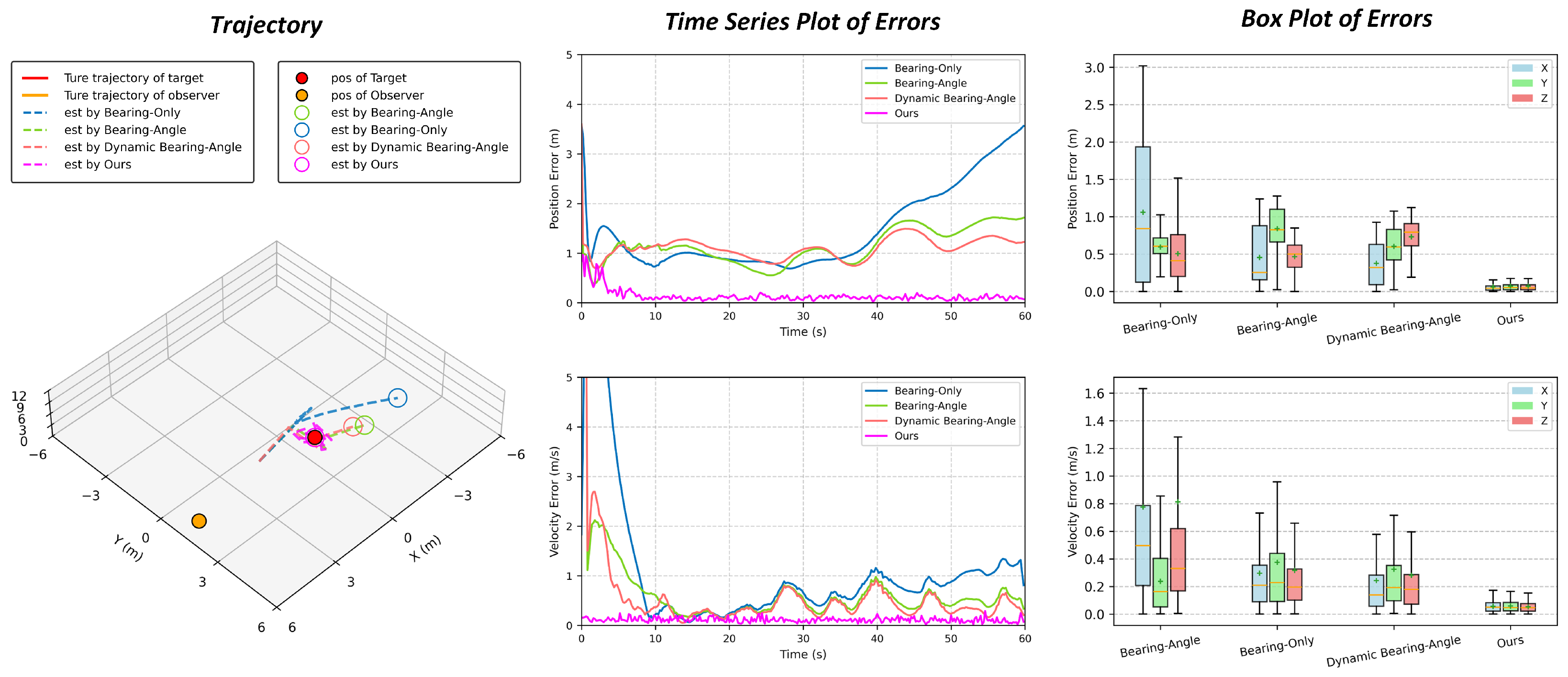
In this scenario, the target and observer are approximately completely stationary, with no changes in bearing or angle throughout the process, except for observation noise disturbances, resulting in zero observability for traditional methods. As shown in Figure 7, the Bearing-only, bearing-angle, and dynamic bearing-angle method all initially remain in a high-error state, then diverge rapidly. In contrast, the trajectory of the proposed method remains aligned with the ground truth, with errors converging rapidly and maintaining stability, showing fluctuations but no drift. This fully verifies the innovation and effectiveness of the proposed method in observability design, providing a more generalizable solution for visual target motion estimation.

Figure 7. Results of experiments in non-motion state observation target scenarios.

4.5. Ablation Experiment

To systematically verify the core design logic of the proposed Multimodal Decoupled Spatiotemporal Adaptive Network (MDSAN), as well as the necessity and rationality of each component, this chapter designs four groups of targeted ablation experiments in three typical observability scenarios (strong, weak, and no observability) of the MS-MAV-ViME dataset. Average Distance Error (ADE) and Average Velocity Error (AVE) are adopted as the core evaluation metrics. By comparing the performance differences of different model configurations, the contributions of key components and parameters are quantified.

To verify the necessity of the two core modules, we compared the performance of three configurations—the complete MDSAN, the model without the MSCN module, and the model without the STAS module—the results of which are shown in Table 3. After removing the MSCN module, the performance degrades significantly, with the worst performance in low-observability scenarios. This is because ordinary convolution cannot achieve the decoupling of visual, physical, and geometric modality features, which are prone to causing cross-modal information contamination, losing the support of the exclusive dynamic characteristics of each modality, and making it difficult to address the lack of observability in scenarios without lateral motion. After removing the STAS module, the performance degradation is even more severe, with obvious error divergence in low-observability and no-observability scenarios. The reason lies in the fact that the spatiotemporal collaborative modeling of the STAS module based on the SSM is the core basis for reconstructing constraints in low-observability scenarios. Without this module, the algorithm cannot capture long-range inter-frame temporal dependencies and cross-modal spatial correlations, and it is difficult to maintain stable estimation relying solely on unimodal features. The above results confirm that the modal decoupling capability of MSCN and the spatiotemporal adaptive modeling capability of STAS form a key synergistic effect. They are the core pillars of MDSAN for breaking through the traditional methods’ reliance on the observer’s high-order motion, and neither of them is dispensable.

Table 3. Results of core module ablation experiment.

Method	Scenario 1		Scenario 2		Scenario 3		Average
	ADE	AVE	ADE	AVE	ADE	AVE	ADE	AVE
MDSAN	0.12	0.18	0.56	0.61	0.06	0.08	0.25	0.29
w/o MSCN	0.27	0.32	0.89	0.95	0.21	0.19	0.46	0.49
w/o STAS	0.35	0.41	1.02	1.13	0.28	0.25	0.55	0.60

To further quantify the independent contributions and synergistic effects of Temporal Mamba and Spatial Mamba in the STAS module and verify the core value of spatiotemporal collaborative modeling, Table 4 designs sub-module ablation experiments in three typical scenarios. By removing the temporal or spatial modeling function separately, we compare the performance differences between the modified models, the complete MDSAN, and the MSCN-only model.

Table 4. STAS sub-module ablation experiment results.

Method	Scenario 1		Scenario 2		Scenario 3		Average
	ADE	AVE	ADE	AVE	ADE	AVE	ADE	AVE
MDSAN	0.12	0.18	0.56	0.61	0.06	0.08	0.25	0.29
MSCN Only	0.35	0.41	1.02	1.13	0.28	0.25	0.55	0.60
w/o Temporal Mamba	0.23	0.29	0.85	0.92	0.20	0.19	0.43	0.47
w/o Spatial Mamba	0.20	0.26	0.78	0.85	0.17	0.16	0.38	0.42

Experimental results show that the performance degrades significantly after removing either sub-module, and the degradation degree is highly correlated with scenario characteristics. The absence of Temporal Mamba has a more prominent impact in low-observability and no-observability scenarios, as it is responsible for capturing the long-term motion trends of MAVs and serves as the key to reconstructing temporal constraints in low-observability scenarios. The removal of Spatial Mamba weakens cross-modal feature complementarity, and its impact on spatial constraint redundancy is more obvious in strong-observability scenarios. The performance of the two sub-modules after ablation lies between that of the complete MDSAN and the MSCN-only model. Moreover, the complete STAS module under the synergistic effect of the two sub-modules achieves the optimal performance, which confirms the design logic: temporal modeling captures motion trends, while spatial modeling enhances feature complementarity.

In summary, as the core components of the STAS module, Temporal Mamba and Spatial Mamba support temporal constraints and spatial feature collaboration, respectively. Their indispensable synergistic effect is the key for MDSAN to break through traditional observability constraints.

Regarding the configuration of modality-specific convolution kernel sizes in the MSCN module, four groups of controlled schemes with different convolution kernel sizes were designed. The experimental results are shown in Table 5.

Table 5. Results of parameter selections for ablation experiment.

Method	Scenario 1		Scenario 2		Scenario 3		Average
	ADE	AVE	ADE	AVE	ADE	AVE	ADE	AVE
$k^{vis}=3,k^{phy}=5,k^{geo}=7$	0.12	0.18	0.56	0.61	0.06	0.08	0.25	0.29
$k^{vis}=3,k^{phy}=3,k^{geo}=3$	0.24	0.29	0.79	0.86	0.18	0.16	0.40	0.44
$k^{vis}=5,k^{phy}=5,k^{geo}=5$	0.18	0.23	0.67	0.73	0.11	0.10	0.32	0.35
$k^{vis}=7,k^{phy}=7,k^{geo}=7$	0.21	0.26	0.72	0.79	0.15	0.13	0.36	0.39

The experimental results show that the average ADE of the unified small-kernel scheme ($k^{vis}=3,k^{phy}=3,k^{geo}=3$) reaches 0.40 m, and the ADE in Scenario 3 increases from 0.06 m to 0.18 m. The reason is that the correlation between the direction angle and opening angle of the geometric modality requires long-range temporal capture, and small kernels cannot cover a sufficient temporal range, leading to insufficient feature extraction of the geometric modality. The average ADE values of the unified medium-kernel scheme ($k^{vis}=5,k^{phy}=5,k^{geo}=5$) and unified large-kernel scheme ($k^{vis}=7,k^{phy}=7,k^{geo}=7$) are 0.32 m and 0.36 m, respectively. For the unified large-kernel scheme, the ADE in Scenario 1 (strong observability) increases from 0.12 m to 0.21 m. This is because the texture features of the visual modality have strong locality, and large kernels will introduce redundant information, undermining the recognizability of local detailed features.

The optimal parameter combination designs kernel sizes differentially according to the temporal dynamic characteristics of different modalities. This design not only avoids cross-modal information contamination but also ensures sufficient feature extraction for each modality, thereby achieving optimal performance across all scenarios.

To quantify the independent contributions and synergistic effects of the three modalities (visual, physical, and geometric) and identify the core modality that breaks observability constraints, Table 6 designs modality ablation experiments in three typical scenarios. By removing individual or combined modalities one by one, we compare the differences in Average Distance Error (ADE) and Average Velocity Error (AVE) between the modified models and the complete MDSAN.

Table 6. Results of modality ablation experiment.

Method	Scenario 1		Scenario 2		Scenario 3		Average
	ADE	AVE	ADE	AVE	ADE	AVE	ADE	AVE
MDSAN	0.12	0.18	0.56	0.61	0.06	0.08	0.25	0.29
w/o Vis	0.23	0.29	0.75	0.82	0.88	0.95	0.62	0.69
w/o Phy	0.17	0.24	0.68	0.74	0.21	0.20	0.35	0.38
w/o Geo	0.19	0.25	0.72	0.78	0.25	0.23	0.39	0.42
w/o Vis + Phy	0.36	0.42	0.98	1.05	1.12	1.20	0.82	0.89
w/o Vis + Geo	0.39	0.45	1.05	1.13	1.25	1.32	0.89	0.97
w/o Phy + Geo	0.30	0.36	0.85	0.90	0.38	0.36	0.51	0.54

Experimental results show under the removal of individual modalities, the performance degradation after removing the visual modality is the most significant, especially in low-observability and no-observability scenarios. This is because the MAV attitude information provided by the visual modality is the core to breaking the traditional single observation dimension and decoupling the coupling relationship between distance and size. The removal of the physical or geometric modality has a minor impact, only weakening motion continuity smoothing in dynamic scenarios, and their modal information can be partially replaced by visual features.

After removing any two modalities, the performance undergoes a cliff-like drop. The error is the largest when both the visual and geometric modalities are missing. This is because the visual modality serves as the core observation dimension, while the geometric modality acts as an auxiliary constraint, and their collaboration constructs the foundation of spatiotemporal constraints.

In summary, the visual modality is the key to breaking observability constraints. The physical and geometric modalities ensure motion continuity and angular assistance. After decoupling and purification by the MSCN module, they provide high-quality inputs for the STAS module. Their synergistic effect is the core logic behind MDSAN’s ability to achieve full-scenario stable estimation.

4.6. Generalization Experiment

To verify the generalization ability of the proposed method under different data distribution scenarios, we designed cross-dataset generalization experiments, focusing on the testing of the motion estimation performance of the method on heterogeneous datasets in two scenarios: without dedicated fine tuning and with dedicated fine tuning. We selected two heterogeneous MAV motion-related datasets—MAV6D and MS-MAV-ViME—to simulate different data distributions corresponding to different models, ensuring the authenticity of generalization verification.

4.6.1. Experimental Details

In the generalization experiments, the model is first trained on the MAV6D dataset, then directly tested on the MS-MAV-ViME dataset; meanwhile, reverse verification is supplemented to cover full cross-scenario settings. Secondly, the model is trained on MAV6D, followed by dedicated fine tuning using 10% random training samples from MS-MAV-ViME (following the training strategy described in the original paper), then tested on the target dataset; reverse verification is also added for this setting.

It should be noted that the public MAV6D dataset does not provide ground-truth velocity labels, so corresponding adjustments are required during training and fine tuning. Specifically, when MAV6D is used as the training set, the core structures of MDSAN (MSCN and STAS) are retained during the training phase, and the final prediction branch is split into a 3D position branch $[P_x,P_y,P_z]$ and a 3D velocity branch $[V_x,V_y,V_z]$. Only the position branch is activated for training at this stage; a loss function ($L_{pos-MES}$) is adopted. The training parameters remain unchanged, but the number of epochs is reduced to 100.

During dedicated fine tuning, the MS-MAV-ViME dataset with velocity labels is used for fine tuning. The model initializes with pre-trained weights obtained from MAV6D, and the velocity branch adopts Xavier initialization, which is only applied to the untrained velocity prediction layer. The loss function is upgraded to joint loss ($L_{total}$) to ensure the continuity of velocity estimation. In terms of the training strategy, the learning rate is reduced to $1\times {10}^{-5}$, which is an order of magnitude lower than that in the pre-training phase, to avoid overwriting the learned position features. The total number of training epochs is 60: the backbone network of the position branch is frozen in the first 10 epochs, with only the velocity branch updated; in the subsequent epochs, all global parameters are unfrozen for overall fine tuning. When the training and test datasets are swapped, the corresponding training and fine-tuning strategies remain consistent with the above and will not be repeated here.

4.6.2. Experimental Results

Experimental results are shown in Table 7. To verify the cross-dataset generalization ability of the proposed motion estimation method, this experiment adopts a controlled design with and without fine tuning to validate the method’s adaptability under heterogeneous data distributions. In the scenario without dedicated fine tuning, whether MAV6D is used as the training set and MS-MAV-ViME as the test set or vice versa, the model does not completely fail due to differences in data distributions and still maintains effective motion estimation accuracy. Although these performance results are significantly lower than the baseline level of training and testing on the same dataset, they are far superior to random-guess results. This indicates that the core motion features learned by the model have a dataset-agnostic nature, the method does not rely on the specific distribution of a single dataset, and its core architecture possesses a solid generalization foundation, verifying the cross-domain transfer potential of the proposed motion estimation method’s core design.

Table 7. Results of cross-dataset generalization experiment.

Training Set	Dedicated Fine Tuning	Test Set	ADE	D-RMSE
MS-MAV-ViME	No	MAV6D	0.41	0.48
MS-MAV-ViME	Yes	MAV6D	0.28	0.33
MAV6D	No	MS-MAV-ViME	0.38	0.43
MAV6D	Yes	MS-MAV-ViME	0.26	0.31

After dedicated fine tuning with only a small number of samples from the target dataset for adaptive training, the performance of both groups of cross-dataset tests is significantly improved and approaches the performance level of training on the same dataset. This result shows that fine tuning only needs to adapt to the distribution differences of heterogeneous datasets, without reconstructing the network architecture, which can quickly enhance the model’s adaptability on the target dataset, fully verifying the method’s cross-dataset adaptation flexibility.

The core architecture of the proposed motion estimation method exhibits significant dataset-agnostic characteristics. Even without dedicated fine tuning, it can still maintain effective performance on heterogeneous datasets, proving its solid generalization foundation. Only a small number of samples from the target dataset is required for dedicated fine tuning to achieve a substantial improvement in cross-dataset motion estimation performance, approaching the level of training on the same dataset. It does not require large-scale annotation of new data or network reconstruction, providing a feasible path for efficiently solving cross-dataset adaptation problems. Meanwhile, high-quality and high-precision source datasets can lay a better foundation for cross-dataset generalization, and the learned robust motion features can be effectively transferred to heterogeneous scenarios, offering an efficient and practical solution to the common dataset transfer problem in practical applications.

4.7. Computational Resource Consumption Experiment

To comprehensively assess the computational efficiency of the proposed MDSAN and benchmark it against traditional motion estimation methods, we performed dedicated computational resource consumption experiments, adopting average frames per second (FPS) as the core metric to characterize real-time inference performance.

The experimental environment was consistent with that described in Section 4.1.1. Table 8 summarizes the average FPS of each method on the two datasets. Experimental results demonstrate that traditional methods achieve extremely high FPS values, owing to their simple explicit modeling logic. In contrast, MDSAN integrates multimodal decoupling (MSCN), spatiotemporal adaptive modeling (STAS), and end-to-end feature fusion, resulting in higher computational complexity but breaking through observability constraints. Although its FPS is significantly lower than that of traditional methods, it still meets the real-time requirements for MAV swarm perception.

Table 8. Average inference FPS of different methods on two datasets.

Method	MAV6D (Average FPS)	MS-MAV-ViME (Average FPS)
Bearing Only	6667.08	6592.35
Baseline Angle	2940.63	2887.41
Dynamic Bearing Angle	2142.72	2093.58
MDSAN	41.28	32.25

For practical MAV swarm applications prioritizing reliability and precision over extreme speed, MDSAN achieves a reasonable balance between high precision, strong robustness, and real-time performance. The trade-off between computational complexity and functional enhancement is justified, as the integrated MSCN (Modality-Specific Convolutional Normalization) and STAS (Spatiotemporal Adaptive State) modules are essential for breaking through the observability limitations of traditional methods.

5. Conclusions

This paper addresses the current imbalance in research focusing on control-heavy and perception-light MAV swarms, as well as the observational limitations of traditional full-vision motion estimation algorithms. It proposes the Multimodal Decoupled Spatiotemporal Adaptive Network (MDSAN). Through modality-specific decoupling and spatiotemporal adaptive modeling, MDSAN overcomes the observational constraints of conventional methods, achieving high-precision 3D relative pose and velocity estimation for dynamically maneuvering MAVs. Specifically, we constructed the MSCN module within the MDSAN framework. By employing modality-specific convolutional kernels, it decouples visual, physical, and geometric features across three modalities. This approach prevents cross-modal information contamination while preserving the dynamic characteristics inherent to each modality. We also developed the STAS module, which constructs a spatiotemporal collaborative modeling framework based on state-space models. By integrating visual and geometric variance-adaptive weights, it reconstructs estimation constraints in low-observability scenarios. The proposed MDSAN avoids reliance on wireless communication and additional hardware costs through a fully visual multimodal fusion approach, meeting the economic and reliability requirements of MAV swarms. Experimental validation in real-world scenarios demonstrates that MDSAN achieves optimal estimation accuracy and stability across traditional observational scenarios—strong, weak, and absent—providing a novel technical approach for MAV swarm perception systems.

References

- Zhou, X.; Wen, X.; Wang, Z.; Gao, Y.; Li, H.; Wang, Q.; Yang, T.; Lu, H.; Cao, Y.; Xu, C. Swarm of micro flying robots in the wild. Sci. Robot. 2022, 7, eabm5954. [Google Scholar] [CrossRef] [Scilit]
- Briñón-Arranz, L.; Seuret, A.; Pascoal, A. Circular formation control for cooperative target tracking with limited information. J. Frankl. Inst. 2019, 356, 1771–1788. [Google Scholar] [CrossRef] [Scilit]
- Gábor, V.; Csaba, V.; Gerg, S.; Tamás, N.; Eiben, A.E.; Tamás, V. Optimized flocking of autonomous drones in confined environments. Sci. Robot. 2018, 3, eaat3536. [Google Scholar] [CrossRef] [Scilit] [PubMed]
- Macwan, A.; Vilela, J.; Nejat, G.; Benhabib, B. A Multirobot Path-Planning Strategy for Autonomous Wilderness Search and Rescue. IEEE Trans. Cybern. 2015, 45, 1784–1797. [Google Scholar] [CrossRef] [Scilit] [PubMed]
- Gao, Y.; Bai, C.; Zhang, L.; Quan, Q. Multi-UAV cooperative target encirclement within an annular virtual tube. Aerosp. Sci. Technol. 2022, 128, 107800. [Google Scholar] [CrossRef] [Scilit]
- Kassabalidis, I.; El-Sharkawi, M.A.; Marks, R.J.; Arabshahi, P.; Gray, A.A. Swarm Intelligence for Routing in Communication Networks. In Proceedings of the IEEE Global Telecommunications Conference, San Antonio, TX, USA, 25–29 November 2001. [Google Scholar]
- Hafez, A.T.; Iskandarani, M.; Givigi, S.N.; Yousefi, S.; Beaulieu, A. UAVs in Formation and Dynamic Encirclement Via Model Predictive Control. IFAC Proc. Vol. 2014, 47, 1241–1246. [Google Scholar] [CrossRef] [Scilit]
- Ferrante, E. A Control Architecture for a Heterogeneous Swarm of Robots. In The Design of a Modular Behavior-based Architecture; Iridia Université Libre de Bruxelles: Bruxelles, Belgique, 2009. [Google Scholar]
- Liu, H.; Liu, D.; Wan, Y.; Lewis, F.L.; Valavanis, K.P. Robust Formation Trajectory Tracking Control for Multiple Quadrotors with Communication Delays. In Robust Formation Control for Multiple Unmanned Aerial Vehicles; CRC Press: Boca Raton, FL, USA, 2022; pp. 37–57. [Google Scholar]
- Schilling, F.; Schiano, F.; Floreano, D. Vision-Based Drone Flocking in Outdoor Environments. IEEE Robot. Autom. Lett. 2021, 6, 2954–2961. [Google Scholar] [CrossRef] [Scilit]
- Tang, Y.; Hu, Y.; Cui, J.; Liao, F.; Lao, M.; Lin, F.; Teo, R. Vision-aided Multi-UAV Autonomous Flocking in GPS-denied Environment. IEEE Trans. Ind. Electron. 2018, 66, 616–626. [Google Scholar] [CrossRef] [Scilit]
- Zhang, P.; Chen, G.; Li, Y.; Dong, W. Agile Formation Control of Drone Flocking Enhanced with Active Vision-Based Relative Localization. IEEE Robot. Autom. Lett. 2022, 7, 8. [Google Scholar] [CrossRef] [Scilit]
- Zheng, C.; Mi, Y.; Guo, H.; Chen, H.; Lin, Z.; Zhao, S. Optimal spatial-temporal triangulation for bearing-only cooperative motion estimation. Automatica 2025, 175, 112216. [Google Scholar] [CrossRef] [Scilit]
- Ning, Z.; Zhang, Y.; Li, J.; Chen, Z.; Zhao, S. A bearing-angle approach for unknown target motion analysis based on visual measurements. Int. J. Robot. Res. 2024, 43, 1228–1249. [Google Scholar] [CrossRef] [Scilit]
- Luo, Y.; Fu, H.; Fu, T.; Cha, H.; Tian, B.; Tang, H.; Liu, F. Dynamic Bearing–Angle for Vision-Based UAV Target Motion Analysis. Sensors 2025, 25, 4396. [Google Scholar] [CrossRef] [Scilit] [PubMed]
- Gu, A.; Goel, K.; Ré, C. Efficiently Modeling Long Sequences with Structured State Spaces. arXiv 2021, arXiv:2111.00396. [Google Scholar]
- Gu, A.; Dao, T. Mamba: Linear-time sequence modeling with selective state spaces. arXiv 2024, arXiv:2312.00752. [Google Scholar]
- Hoelzer, H.; Johnson, G.W.; Cohen, A.O. Modified Polar Coordinates-The Key to Well Behaved Bearings Only Ranging; Report Number: IBM IR&D Report 78-M19-0001A; IBM: Manassas, VA, USA, 1978. [Google Scholar] [CrossRef]
- Aidala, V.J. Kalman Filter Behavior in Bearings-Only Tracking Applications. IEEE Trans. Aerosp. Electron. Syst. 2007, 15, 29–39. [Google Scholar] [CrossRef] [Scilit]
- Lin, X.; Kirubarajan, T.; Bar-Shalom, Y.; Maskell, S.; England, Q.M. Comparison of EKF, pseudomeasurement, and particle filters for a bearing-only target tracking problem. Proc. SPIE-Int. Soc. Opt. Eng. 2007, 4728, 240–250. [Google Scholar]
- Fogel, E.; Gavish, M. Nth-order dynamics target observability from angle measurements. IEEE Trans. Aerosp. Electron. Syst. 1988, 24, 305–308. [Google Scholar] [CrossRef] [Scilit]
- He, S.; Shin, H.S.; Tsourdos, A. Trajectory Optimization for Target Localization with Bearing-Only Measurement. IEEE Trans. Robot. 2019, 35, 16. [Google Scholar] [CrossRef] [Scilit]
- Li, J.; Ning, Z.; He, S.; Lee, C.H.; Zhao, S. Three-Dimensional Bearing-Only Target Following via Observability-Enhanced Helical Guidance. IEEE Trans. Robot. 2023, 39, 18. [Google Scholar] [CrossRef] [Scilit]
- Zhang, L.; Xie, C.; Kitahara, I. DP-AMF: Depth-Prior–Guided Adaptive Multi-Modal and Global–Local Fusion for Single-View 3D Reconstruction. J. Imaging 2025, 11, 246. [Google Scholar] [CrossRef] [Scilit]
- Sandler, M.; Howard, A.; Zhu, M.; Zhmoginov, A.; Chen, L.C. MobileNetV2: Inverted Residuals and Linear Bottlenecks. In Proceedings of the 2018 IEEE/CVF Conference on Computer Vision and Pattern Recognition, Salt Lake City, UT, USA, 18–23 June 2018. [Google Scholar]
- Redmon, J.; Farhadi, A.; Team, Y.D. YOLOv11: An Overview of the Key Architectural Enhancements. arXiv 2024, arXiv:2410.17725. [Google Scholar] [CrossRef] [Scilit]
Disclaimer/Publisher’s Note: The statements, opinions and data contained in all publications are solely those of the individual author(s) and contributor(s) and not of MDPI and/or the editor(s). MDPI and/or the editor(s) disclaim responsibility for any injury to people or property resulting from any ideas, methods, instructions or products referred to in the content. |
© 2026 by the authors. Licensee MDPI, Basel, Switzerland. This article is an open access article distributed under the terms and conditions of the Creative Commons Attribution (CC BY) license.