Aboveground Biomass Inversion of Farmland Shelterbelts Across Degradation Levels Using UAV LiDAR–Multispectral Fusion: A Case Study in Xinjiang, China

Highlights

What are the main findings?

• Fusion of UAV-LiDAR structural metrics and multispectral vegetation indices consistently improved agreement with reference AGB compared with LiDAR-only or multispectral-only models, and the improvement became more pronounced under severe degradation where geometry–biomass coupling weakens. The support vector regression (SVR) algorithm fusing UAV-LiDAR structural metrics and multispectral vegetation indices achieved the best overall performance among the tested algorithms.
• The fused SVR achieved the highest accuracy (R² = 0.846/0.848/0.718 for healthy/moderately/severely degraded belts)

What are the implications of the main findings?

• These results indicate that a non-destructive UAV fusion workflow can provide operational, plot-scale AGB diagnostics to support maintenance prioritization and restoration decisions for degraded shelterbelts, especially when structural proxies alone become unreliable under canopy fragmentation and dieback. While the framework is methodologically general, the fitted parameters (including ρ and model weights) remain site- and season-specific and should be transferred only with additional calibration and independent biomass validation.

Abstract

Accurate aboveground biomass (AGB) estimation of farmland shelterbelts is critical for evaluating shelterbelt degradation and guiding restoration in arid agricultural landscapes. However, satellite-based retrieval is challenging for narrow linear belts affected by strong edge effects and canopy gaps under degradation. Here we developed a plot-scale Unmanned Aerial Vehicle (UAV) workflow that fuses Light Detection and Ranging (LiDAR) structural metrics and multispectral vegetation indices to estimate individual-tree AGB for Populus euphratica Olivier (Xinjiang poplar) shelterbelts in Tiemenguan, Xinjiang, China. Field measurements were collected in October 2024 from three belts representing healthy, moderately degraded, and severely degraded conditions (n = 135 trees; 45/50/40). Because destructive sampling was infeasible, AGB was derived as allometry-based reference values, with a prior-constrained scale factor (ρ) used to ensure physically plausible ranges. We compared multiple linear regression, random forest, and Support vector regression (SVR) models under LiDAR-only, multispectral-only, and fused inputs. Fusion consistently improved agreement with reference AGB, and the fused SVR achieved the best performance (test R² = 0.846/0.848/0.718 for healthy/moderately/severely degraded belts). The workflow highlights spectral–structural complementarity for degraded shelterbelts, while broader deployment requires local calibration and independent biomass validation.

1. Introduction

Farmland shelterbelts (windbreaks) in arid agricultural regions regulate wind, temperature, moisture and soil conditions, thereby stabilizing crop production and delivering ecological co-benefits [1,2,3]. In Northwest China, long-term construction under the “Three-North” Shelterbelt Program has created extensive shelterbelt networks, yet many belts are experiencing stand aging and degradation [4,5,6]. Quantitative indicators that can support timely maintenance and restoration prioritization are therefore increasingly needed in operational management [7,8].

Unlike closed forests, farmland shelterbelts are typically narrow, linear formations embedded in an agricultural matrix, characterized by strong edge effects, high within-belt heterogeneity, and frequent disturbances [9]. These features complicate biomass retrieval because canopy structure and physiological conditions can vary markedly over short distances [10,11,12]. In this study, “degradation level” refers to a gradient of structural and vitality decline (e.g., increased crown gaps and dieback, reduced crown width and height, and higher mortality/branch dieback occurrence), which in arid environments may be linked to chronic water deficit, soil salinity and management constraints [13]. Such degradation can weaken the empirical relationship between geometric structure and aboveground biomass (AGB), making shelterbelts a distinct research object that requires tailored estimation strategies [14,15].

Traditional AGB acquisition relies on field surveys and allometric equations, and destructive sampling is often required for local calibration; however, destructive sampling is usually infeasible in operational shelterbelts because of their protective function and management constraints [16,17]. Remote sensing has become an important alternative for non-destructive biomass inversion, but satellite observations often face limitations in shelterbelts due to mixed pixels, insufficient spatial detail for narrow belts, and constrained revisit schedules for timely assessments [8]. Unmanned aerial vehicles (UAVs) provide flexible, high-resolution observations and can support fine-scale monitoring aligned with belt-level management needs [18,19].

UAV-LiDAR captures three-dimensional canopy structure (e.g., height, crown geometry and cover), whereas multispectral data provide vegetation indices reflecting canopy vigor and stress responses [20,21,22]. Combining structural and spectral features can improve AGB estimation, particularly under heterogeneous or disturbed conditions where a single data source becomes unstable. Nevertheless, shelterbelt-specific evidence across multiple degradation levels remains limited, and robust calibration is challenging when destructive biomass measurements are not available, which may introduce systematic bias if allometry is used as the reference.

To address these gaps, we selected three Populus euphratica Olivier shelterbelts representative of three degradation levels, i.e., healthy, moderately degraded and severely degraded, in an arid reclamation area of Xinjiang (surveyed in October 2024) and developed an individual-tree AGB estimation workflow by fusing UAV-LiDAR structural metrics with multispectral vegetation indices [23,24,25]. We tested multiple modeling strategies (multiple linear regression, MLR; random forest regression, RFR; and support vector regression, SVR) with dimensionality reduction and feature selection, and produced plot-scale AGB maps for belt-level diagnosis. We hypothesize that (H1) fused structural–spectral features provide more robust AGB estimates than single-source features across degradation levels; and (H2) the benefit of multispectral information becomes more pronounced as degradation increases because purely geometric proxies become less reliable. Our results demonstrate the feasibility of a non-destructive, plot-scale framework; extension to broader regions or seasons should be conducted with additional sites and independent biomass validation.

2. Materials and Methods

2.1. Materials

2.1.1. Study Area

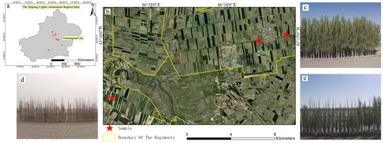
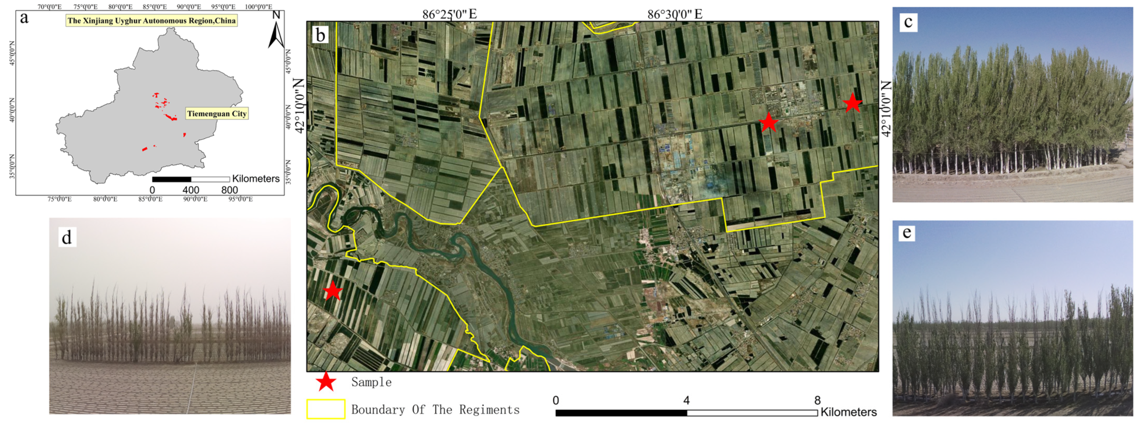
The study area is located in the Yanqi Reclamation Area of Tiemenguan City, Second Division of the Xinjiang Production and Construction Corps (42°10′16″ N, 86°34′06″ E), situated at the southern foot of the Tianshan Mountains in the Yanqi Basin, within the Peacock River watershed. The elevation is approximately 1006 m, and the primary terrain consists of plains, with a continental temperate desert climate. The annual average temperature is 8.6 °C, with a frost-free period of approximately 177 days and an average annual precipitation of 59.2 mm. The forest resources in the area are primarily composed of artificial farmland shelterbelts dominated by Populus euphratica Olivier (Xinjiang poplar). The location and sampling design are shown in Figure 1.

Figure 1. Overview of the study area: (a) Tiemenguan City, Second Division of the Xinjiang Production and Construction Corps; (b) Sample distribution map; (c) Healthy status; (d) Severely degraded status; (e) Moderately degraded status.

2.1.2. Degradation Level Classification

Shelterbelt degradation levels were classified according to the national standard GB/T 44351-2024 (Technical Specification for Degraded Forest Restoration) [26]. In this standard, moderate degradation is defined when shelterbelt porosity is between 0.6 and 0.8, or when the maximum continuous belt-break length is more than twice the mean tree height, and the total missing-belt length accounts for more than 20% but not more than 50% of the overall belt length. Severe degradation is defined when shelterbelt porosity is 0.8 or higher, or when the maximum continuous belt-break length is more than twice the mean tree height and the total missing-belt length accounts for more than 50% of the overall belt length.

Here, porosity refers to the proportion of void space within the shelterbelt relative to the total enclosed belt volume. The maximum continuous belt-break length describes the longest uninterrupted gap along the shelterbelt, and the missing-belt length proportion represents the ratio of the cumulative missing-belt length to the total belt length. Based on these criteria, three belts representing healthy, moderately degraded, and severely degraded conditions were selected for subsequent field survey and UAV data acquisition. Belts that did not meet the criteria for moderate or severe degradation were categorized as healthy.

To make the degradation classification reproducible, we summarize the measured/derived indicators for each shelterbelt (maximum continuous belt-break length and missing-belt proportion) together with the corresponding GB/T 44351-2024 thresholds in Table 1.

Table 1. Quantitative indicators used for shelterbelt degradation classification (GB/T 44351-2024).

Degradation Level	Max Belt-Break Length (m)	Total Belt-Break Length (m)	Mean Tree Height (m)	Belt Length (m)	Missing-Belt Proportion (%)
Healthy	0	0	22.43	237	0
Moderately degraded	27	48	17.08	218	22.02
Severely degraded	42	137	15.10	204	67.16

2.1.3. Field Measurements and Prior-Constrained Reference AGB

Ground measurements were conducted in October 2024 along the three shelterbelt segments. Trees were sampled at 5 m intervals along the belt centreline; at each interval, the nearest dominant tree was measured, resulting in 45 (healthy), 50 (moderately degraded), and 40 (severely degraded) trees (n = 135). Tree height (H, m) was measured using an SNDWAY telescope rangefinder, diameter at breast height (D, cm; 1.3 m above ground) was measured with a diameter tape, and canopy width (C, m) was calculated as the average of two perpendicular crown diameters.

Individual-tree AGB was first estimated using a published allometric equation for Populus euphratica Olivier plantations in arid Xinjiang (Equation (1)), driven by field-measured D and tree height. Throughout the manuscript, this allometry-based AGB of the i-th tree is denoted as AGB_eq,i and serves as the initial non-destructive estimate.

To constrain the above estimates within physically plausible ranges, we derived the stem volume (V_i) from field measurements using a shape-coefficient formulation (k = 0.3927) (Equation (2)). Based on V_i, the feasible biomass interval [AGB_min,_i, AGB_max,_i] was computed using prior ranges of wood density (WD) and biomass expansion factor (BEF2) (Equations (3)–(4)). IPCC default values (WD = 0.35 t d.m. m⁻³; BEF2 = 1.4) [27,28] were used as the central priors, while conservative bounds (WD: 0.30–0.40 t d.m. m⁻³; BEF2: 1.2–1.6) were adopted to account for site variability.

A degradation-specific scale factor (ρ) was estimated separately for moderately and severely degraded shelterbelts by minimizing the mismatch between the scaled allometric estimates (ρ·AGB_eq,i) and the feasible interval [AGB_min,_i, AGB_max,_i]. A regularization term (λ = 1.0) was introduced to discourage over-correction. The resulting ρ estimates are reported as the median with uncertainty bounds (Table 2). For the healthy shelterbelt, we fixed ρ = 1.0. For clarity and to facilitate subsequent analyses, we also provide degradation-specific expressions of the scaled allometric reference AGB: Equations (6) and (7) correspond to the moderately degraded (AGB_M,_i) and severely degraded (AGB_S,_i) forms of Equation (1), where the multipliers 0.8 and 0.7 are rounded approximations of the median ρ values (0.7996 and 0.7025). All subsequent analyses use tree-level reference AGB (AGB_ref) computed with the unrounded ρ (including its Monte Carlo uncertainty).

Table 2. Monte Carlo-derived uncertainty bounds of the scale coefficient (ρ) by degradation level.

Degradation Level	n (Trees)	ρ Median	ρ Q1	ρ Q3	ρ IQR	ρ 2.5%	ρ 97.5%
Healthy	45	1.0000	1.0000	1.0000	0.0000	1.0000	1.0000
Moderately degraded	50	0.7996	0.7231	0.8804	0.2359	0.6104	1.0377
Severely degraded	40	0.7025	0.6350	0.7731	0.2168	0.5361	0.9112

Uncertainty in ρ and reference AGB was quantified using Monte Carlo sampling (1000 iterations) by perturbing prior parameters within plausible ranges (WD: 0.30–0.40 t d.m. m⁻³; BEF2: 1.2–1.6; k: 0.35–0.45). We summarize the Monte Carlo results using the median, interquartile range (IQR), and percentile-based uncertainty bounds (2.5–97.5%). In the following analyses, the scaled allometry-based labels are referred to as reference AGB (AGB_ref), rather than destructively measured biomass.

Notably, the estimation of ρ and AGB_ref relies exclusively on field measurements and prior parameter ranges, and does not use UAV LiDAR structural metrics or multispectral predictors. This design reduces circularity, so model evaluation reflects the ability of remote-sensing features to predict field-constrained reference AGB.

Using the above procedure, reference AGB for each tree was calculated, and the descriptive statistics of field measurements and reference AGB by degradation level are summarized in Table 3.

$${AGB}_{eq,i}=0.1221{\left({D_i}^2{H}_i\right)}^{0.7813}$$

(1)

$$V_i=k\cdot D_i^2\cdot H_i$$

(2)

$${AGB}_{min,i}=V_i\cdot W{D}_{low}\cdot BE{F}_{low}$$

(3)

$$AG{B}_{max,i}=V_i\cdot W{D}_{high}\cdot BE{F}_{high}$$

(4)

$${\rho }^{*}=\underset{\rho }{arg min}[{\displaystyle \sum _{i=1}^n}{\left(max\right\{0,\rho \cdot {AGB}_{eq,i}-{AGB}_{max,i}\left\}\right)}^2+{\displaystyle \sum _{i=1}^n}{\left(max\right\{0,{AGB}_{min,i}-\rho \cdot {AGB}_{eq,i}\left\}\right)}^2+\lambda {(\rho -1)}^2]$$

(5)

$${\mathit{AGB}}_{M,i}=0.8\times 0.1221{\left({D_i}^2{H}_i\right)}^{0.7813}$$

(6)

$${\mathit{AGB}}_{S,i}=0.7\times 0.1221{\left({D_i}^2{H}_i\right)}^{0.7813}$$

(7)

Table 3. Descriptive statistics of field-measured tree attributes and reference AGB by degradation level.

Degradation Level	Parameters	Minimum	Mean	Maximum	STD
Healthy	H (m)	12.80	22.43	26.54	2.95
	D (cm)	14.00	34.90	56.98	9.32
	C (m)	3.15	6.74	13.4	2.10
	AGB (kg)	55.45	378.91	872.98	186.89
Moderately Degraded	H (m)	8.83	17.08	26.21	4.33
	D (cm)	12.15	21.35	35.00	5.11
	C (m)	1.00	4.89	10.22	2.13
	AGB (kg)	26.54	153.52	285.76	57.44
Severely Degraded	H (m)	8.63	15.10	20.90	2.79
	D (cm)	11.46	20.44	34.50	6.08
	C (m)	1.36	3.90	8.82	1.56
	AGB (kg)	19.87	73.65	160.88	35.30

2.1.4. UAV Multispectral Data Acquisition

UAV data acquisition was conducted in the study area on 23 October 2024. The multispectral mission was planned with approximately 80% forward overlap and 70% side overlap to improve tie-point matching and orthomosaic quality. A total of 145, 186, and 162 multispectral images were collected for the healthy, moderately degraded, and severely degraded shelterbelts, respectively. The multispectral and LiDAR surveys were conducted on the same date (23 October 2024) under cloud-free conditions; however, the two sensors were deployed in two separate UAV flight missions (two sorties) rather than simultaneously. Both missions were completed consecutively within the same day to minimize temporal mismatch between canopy structure and spectral responses. Aerial imagery was captured between 13:00 and 15:00, with clear skies, ample sunlight, and minimal wind on the day of the flight. The flight was conducted using the Feima D2000S UAV (Shenzhen Feima Robotics Co., Ltd., Shenzhen, China), which has a standard takeoff weight of 2.8 kg, a maximum payload capacity of 1.2 kg, a top speed of 20 m/s, and a flight endurance of up to 74 min. These parameters enabled the UAV to cover a large area in a single flight mission, improving data collection efficiency. The UAV was equipped with a YUSENSE MS600 multispectral sensor (Changguang Yuchen Information Technology and Equipment (Qingdao) Co. Ltd., Qingdao, China), featuring six 1.2-megapixel multispectral channels (Table 4). The data format consisted of multi-channel .jpg grayscale images.

Table 4. Band parameters of MS600 multispectral sensor.

Spectral Channels	Spectral Properties	Center Wavelength/nm
Band1	Blue	450
Band2	Green	555
Band3	Near-infrared	840
Band4	Red	660
Band5	Red−Edge 1	720
Band6	Red−Edge 2	750

2.1.5. UAV LiDAR Data Acquisition

The UAV LiDAR survey was conducted on 23 October 2024 as an independent flight mission (separate sortie) from the multispectral acquisition, and the two missions were coordinated to ensure consistent canopy status for subsequent data fusion. The UAV was equipped with the D-LiDAR2100 sensor, which enables the acquisition of high-precision terrain, vegetation structure, and soil surface feature observations (Table 5), and works in conjunction with the integrated data processing software “Zhijiguang”. This UAV remote sensing platform is equipped with a Position and Orientation System (POS) that enables real-time acquisition of image data. Additionally, the UAV features an integrated RTK system, eliminating the need for base station setup. The flight height was set to 60 m for the experiment. After reaching the flight altitude, the UAV followed a vertical zigzag flight pattern, autonomously capturing images at equal intervals through the UAV Manager software on a laptop. The flight had a longitudinal overlap of 80% and a lateral overlap of 70%.

Table 5. D-LiDAR2100 LiDAR sensor parameters.

Performance Indicator	Value
Flight Altitude	50–200 m
Flight Speed	13.5 m/s
Point Frequency	240 kPts/s
Measurement Range	190 m at 10% reflectance and 100 klx illumination
Laser Field of View	70.4° (Horizontal)/77.2° (Vertical)
Accuracy of Results	±5 cm at 100 m (Horizontal)

2.2. Data Preprocessing

2.2.1. LiDAR Point Cloud Data Processing

LiDAR360 (Beijing Green Valley Technology Co. Ltd., Beijing, China) is a specialized LiDAR (Light Detection and Ranging) data processing software. The DSM generation process based on LiDAR begins with preprocessing the LiDAR data using the UAV Manager platform. The point cloud density is set to the original sampling rate, with 100% of the point cloud used for processing. The effective range of the point cloud is set to 300 m, and the output data is in LAS format. Next, point cloud filtering is performed using LiDAR360 to remove noise. The software automatically calculates the search radius, with relative error (sigma) used as the denoising criterion. Points within a search radius of fewer than four are considered isolated points and removed. Subsequently, LiDAR360 is used for object classification of the point cloud data and for converting the LAS dataset into a raster format, classifying the points into ground and non-ground points. A resolution of 0.5 m was set to generate the DSM and DEM from the LiDAR data source.

2.2.2. Multispectral Image Stitching

Multispectral images from each flight were processed in Pix4D Mapper (Pix4D SA, Prilly, Switzerland) using the standard multispectral photogrammetric workflow. In total, 145, 186, and 162 multispectral frames were processed for the healthy, moderately degraded, and severely degraded shelterbelts, respectively. All frames acquired along each shelterbelt were imported and aligned through automatic keypoint matching, followed by camera self-calibration, bundle adjustment, dense point-cloud reconstruction, and orthorectification. Radiometric normalization was applied to reduce illumination differences among frames, and band-specific orthomosaics were generated and co-registered to produce a stacked reflectance mosaic. These ortho-products were used to compute vegetation indices and extract plot-level spectral features (Section 2.2.4).

2.2.3. Single Tree Segmentation and Crown Extraction

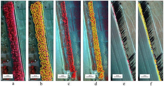
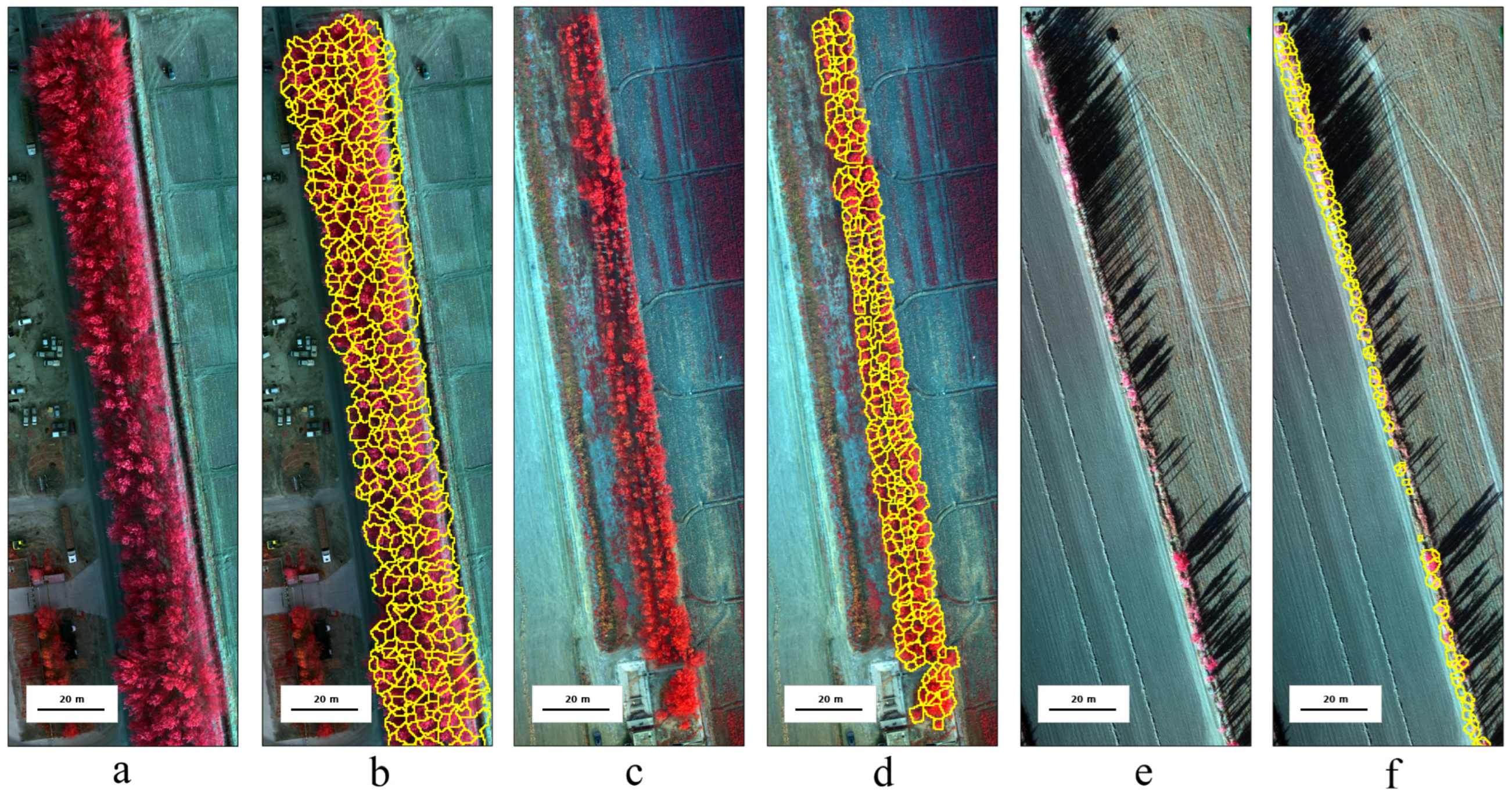
The construction of a Canopy Height Model (CHM) based on LiDAR point clouds, followed by seed point extraction for individual tree segmentation, has become the mainstream approach for obtaining individual tree-scale forest parameters [29,30]. In LiDAR360, the preprocessed point cloud is used to generate a Digital Surface Model (DSM) and a Digital Elevation Model (DEM), and their difference is used to obtain the CHM, which characterizes the spatial distribution of canopy height. The local maxima of the CHM are then used as seed points for tree location, and the “Seed Point-based Segmentation” tool is employed for individual tree segmentation. The segmentation results are manually verified and corrected, with the individual tree crown boundaries vectorized to form canopy polygons for subsequent parameter extraction, as shown in Figure 2. In parallel, the identification number, location, canopy width, and tree height of each tree after segmentation are recorded. The errors between the tree height and canopy width extracted from individual tree segmentation and the field measurements are shown in Table 6.

Figure 2. (a) Multispectral imagery of the healthy state; (b) CHM-based individual tree segmentation results for the healthy state; (c) Multispectral imagery of the moderately degraded state; (d) CHM-based individual tree segmentation results for the moderately degraded state; (e) Multispectral imagery of the severely degraded state; (f) CHM-based individual tree segmentation results for the severely degraded state. Scale bar: 20 m. All panels are based on actual UAV measurement data from this study, and are not Google Earth base maps.

Table 6. Accuracy of LiDAR-derived height and crown width against field measurements.

Degradation Level	Parameters	Minimum	Mean	Maximum	STD	R2	RMSE
Healthy	H (m)	15.89	23.87	34.79	6.10	0.99	0.65
	C (m)	4.5	7.38	16.5	2.34	0.86	1.19
Moderately degraded	H (m)	9.86	17.48	23.11	3.40	0.97	0.64
	C (m)	1.00	3.45	5.5	1.20	0.90	0.58
Severely degraded	H (m)	12.50	15.22	28.19	4.79	0.99	0.57
	C (m)	1.00	3.70	9.8	2.03	0.91	0.62
Total	H (m)	9.86	18.86	34.79	2.84	0.98	0.79
	C (m)	1.00	4.84	16.50	1.32	0.89	0.87

2.2.4. Feature Extraction

Vegetation index characteristics reflect the growth status of surface vegetation and are important variables for constructing biomass estimation models. To estimate the biomass of Populus euphratica Olivier shelterbelts in the study area, this study used ENVI 5.6 software to extract 26 vegetation index features from UAV multispectral data to construct the biomass model. Detailed information is provided in Table 7.

Table 7. Common vegetation indices and their calculation formulas.

Features		Formula	Reference
Vegetation indices	Cig	$(\mathrm{b}3 / \mathrm{b}2)-1$	[31]
	CIVE	$0.441 \times \mathrm{b}4-0.881 \times \mathrm{b}2+0.385\times \mathrm{b}1+18.787$	[32]
	DVI	$\mathrm{b}3-\mathrm{b}4$	[32]
	EVI	$2.5 \times (\mathrm{b}3-$$\mathrm{b}4\left)\right(\mathrm{b}3 + 6 \times \mathrm{b}4-$7.5 × b1 + 1)	[21]
	EVI2	${\displaystyle \frac{2.5\times (\mathrm{b}3-\mathrm{b}4)}{(\mathrm{b}3+\mathrm{b}4+1)}}$	[33]
	EXG	$2\times \mathrm{b}2-\mathrm{b}4-\mathrm{b}1$	[34]
	EXGR	${\displaystyle \frac{(1.4\times \mathrm{b}4-\mathrm{b}2)}{(\mathrm{b}4+\mathrm{b}2+\mathrm{b}1)}}$	[35]
	EXR	${\displaystyle \frac{(1.4\times \mathrm{b}4-\mathrm{b}2)}{(\mathrm{b}4+\mathrm{b}2+\mathrm{b}1)}}$	[35]
	FDI	$\mathrm{b}3-(\mathrm{b}2+\mathrm{b}4)$	[36]
	GNDVI	${\displaystyle \frac{(\mathrm{b}3-\mathrm{b}2)}{(\mathrm{b}3+\mathrm{b}2)}}$	[32]
	LCI	${\displaystyle \frac{(\mathrm{b}3-\mathrm{b}5)}{(\mathrm{b}3+\mathrm{b}5)}}$	[37]
	MGRVI	${\displaystyle \frac{({\mathrm{b}2}^2-{\mathrm{b}4}^2)}{({\mathrm{b}2}^2+{\mathrm{b}4}^2)}}$	[38]
	MSAVI	${\displaystyle \frac{2\times \mathrm{b}3+1-\sqrt{{(2\times \mathrm{b}3+1}^2-8\times (\mathrm{b}3-\mathrm{b}4))}}{2}}$	[39]
	NBI	${\displaystyle \frac{\mathrm{b}1}{(\mathrm{b}4+\mathrm{b}1+\mathrm{b}2)}}$	[32]
	NDRE1	${\displaystyle \frac{(\mathrm{b}3-\mathrm{b}5)}{(\mathrm{b}3+\mathrm{b}5)}}$	[40]
	NDRE2	${\displaystyle \frac{(\mathrm{b}3-\mathrm{b}6)}{(\mathrm{b}3+\mathrm{b}6)}}$	[41]
	NDVI	${\displaystyle \frac{(\mathrm{b}3-\mathrm{b}4)}{(\mathrm{b}3+\mathrm{b}4)}}$	[42]
	NGI	${\displaystyle \frac{\mathrm{b}2}{(\mathrm{b}4+\mathrm{b}1+\mathrm{b}2)}}$	[43]
	NGRDI	${\displaystyle \frac{(\mathrm{b}2-\mathrm{b}4)}{(\mathrm{b}2+\mathrm{b}4)}}$	[44]
	NRI	${\displaystyle \frac{\mathrm{b}4}{(\mathrm{b}4+\mathrm{b}1+\mathrm{b}2)}}$	[32]
	OSAVI	${\displaystyle \frac{1.16\times (\mathrm{b}3-\mathrm{b}4)}{(\mathrm{b}3+\mathrm{b}4+0.16)}}$	[20]
	RGRI	${\displaystyle \frac{\mathrm{b}4}{\mathrm{b}2}}$	[45]
	SAVI	${\displaystyle \frac{(\mathrm{b}3-\mathrm{b}4)}{(\mathrm{b}3+\mathrm{b}4+1.5)}} \times 1.5$	[46]
	SR	${\displaystyle \frac{\mathrm{b}3}{\mathrm{b}4}}$	[47]
	TNDVI	$\sqrt{0.5+{\displaystyle \frac{(\mathrm{b}3-\mathrm{b}4)}{(\mathrm{b}3+\mathrm{b}4)}}}$	[48]
	VDVI	${\displaystyle \frac{(2 \times \mathrm{b}2-\mathrm{b}4-\mathrm{b}1)}{(\mathrm{b}22 \times \mathrm{b}2+\mathrm{b}4+\mathrm{b}1)}}$	[49]

2.2.5. Vegetation Index Selection

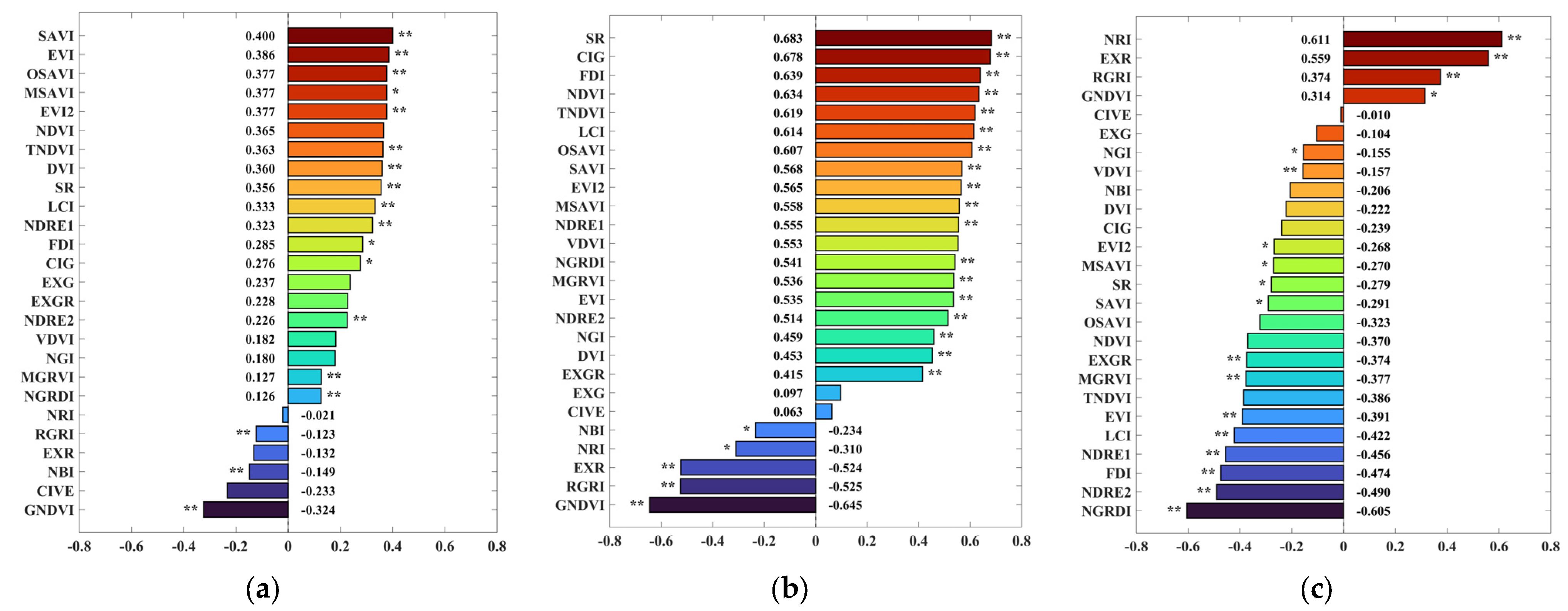
To reduce redundancy among vegetation indices and identify informative predictors, Pearson’s correlation analysis was performed separately within each degradation level. The Pearson correlation coefficient (r) between each vegetation index and the reference AGB (AGB_ref) was calculated to quantify bivariate association. In addition, collinearity among indices was evaluated using pairwise correlations; for highly collinear index pairs (e.g., ∣r∣ > 0.90), only one index was retained to avoid redundancy (the one with the larger ∣r∣ with AGB_ref, or with clearer biophysical interpretability when ∣r∣ was similar). Significance was assessed using two-tailed tests (p < 0.05 * and p < 0.01 **). Full correlation results for all 26 indices are provided in Figure 3. PCA was then applied to the retained vegetation indices within each degradation level to further reduce multicollinearity and to summarize shared variance. Components with eigenvalues > 1 were retained (Kaiser criterion), and the loading matrix was used to interpret the retained components. For parsimony in subsequent modeling, the vegetation index with the highest absolute loading within each retained component was selected as a representative index (reported in Table 8).

Figure 3. Pearson correlation coefficient and significance between AGB and vegetation index of farmland shelterbelts with different degradation degrees: (a) Healthy state; (b) Moderately degraded state; (c) Severely degraded state. Asterisks indicate statistical significance (* p < 0.05; ** p < 0.01).

Table 8. Cumulative variance explained by vegetation indices under different degradation levels.

Degradation Level	Principal Component	Total	Variance Explained (%)	Cumulative Variance Explained (%)
Healthy	OSAVI	14.781	56.848	56.848
	RGRI	6.986	26.868	83.717
	TNDVI	1.731	6.657	90.374
	NDRE2	1.394	5.361	95.735
Moderately degraded	NDVI	18.975	82.499	82.499
	NDRE2	1.774	7.711	90.21
	RGRI	1.103	4.794	95.004
Severely degraded	SAVI	19.584	75.325	75.325
	TNDVI	3.111	11.965	87.289
	NRI	1.291	4.964	92.253

2.3. Modeling Methods

Three machine learning methods were used: multiple linear regression (MLR), random forest regression (RFR), and support vector regression (SVR). Within each degradation class, samples were split into training (70%) and testing (30%) sets using stratified random sampling. All models were trained on the training set and evaluated on the held-out test set. For fair comparison, LiDAR-only, multispectral-only, and fused inputs used the same split.

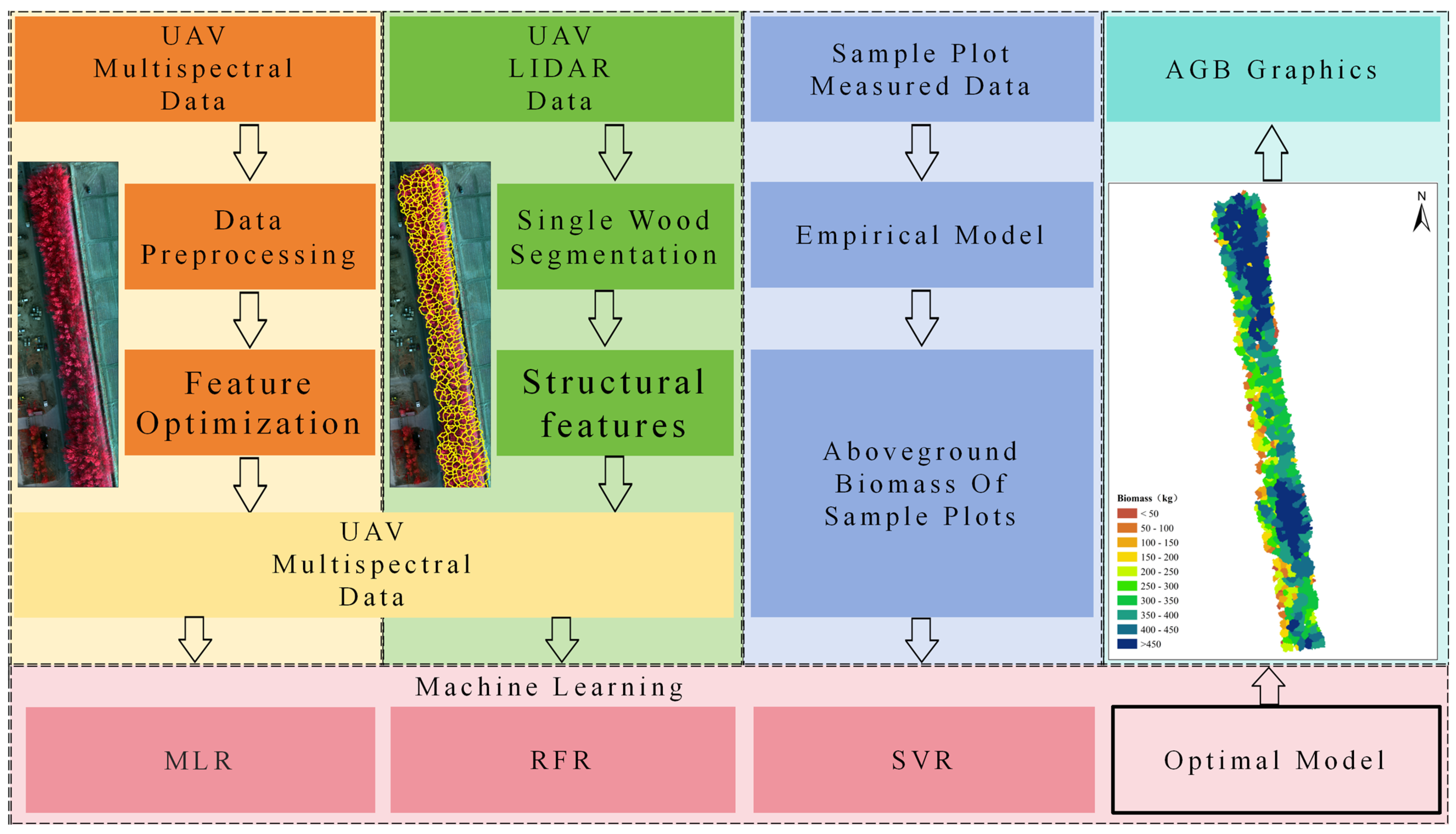
MLR establishes a linear equation to effectively handle multiple independent variables, predict the dependent variable, and use regression coefficients to represent the impact of each independent variable on the dependent variable [50]. RFR combines multiple random decision trees to improve prediction accuracy by averaging their performance. This method grows numerous decision trees on different data subsets and randomly selects predictor variables at each node, thereby integrating the output of individual trees [51]. SVR is an extension of the Support Vector Machine method, designed for regression problems, using kernel functions to handle nonlinear relationships. It improves prediction accuracy by optimizing hyperparameters such as the penalty coefficient C, kernel width γ, and insensitive bandwidth ε [52,53,54]. In this study, the key parameters of the RFR model were optimized using grid search, with the number of trees (ntree) set to 500 and the maximum tree depth (max_depth) set to 15. SVR used a Radial Basis Function (RBF) kernel, with the optimal hyperparameter configuration determined through Bayesian optimization. The overall workflow of feature selection, model training, and evaluation is summarized in Figure 4.

Figure 4. Technical flow charts.

2.4. Model Accuracy Evaluation Metrics

Model performance was evaluated on the held-out test set using R², RMSE, and rRMSE. When needed, non-parametric bootstrap resampling of the test-set residuals was used to derive 95% confidence intervals for ΔRMSE/ΔrRMSE between models. To avoid overclaiming statistical significance when comparing models, performance differences are interpreted primarily in a practical sense; when needed, non-parametric paired bootstrap resampling of prediction residuals can be used to derive 95% confidence intervals for ΔRMSE/ΔrRMSE between models.

$${\mathrm{R}}^2={\displaystyle \frac{{\sum }_{\mathrm{i}=1}^{\mathrm{N}}{({\mathrm{Y}}_{\mathrm{i}}^{\prime }-\overline{\mathrm{Y}})}^2}{{\sum }_{\mathrm{i}=1}^{\mathrm{N}}{({\mathrm{Y}}_{\mathrm{i}}-\overline{\mathrm{Y}})}^2}}$$

(8)

$$\mathrm{RMSE}=\sqrt{{\displaystyle \frac{{\sum }_{\mathrm{i}=1}^{\mathrm{N}}{({\mathrm{Y}}_{\mathrm{i}}-{\mathrm{Y}}_{\mathrm{i}}^{\prime })}^2}{\mathrm{N}}}}$$

(9)

In the equation, $Y_i$ represents reference AGB derived from allometry (with ρ when applied), $Y_i^{\prime }$ represents the aboveground biomass estimated by the model, $\overline{Y}$ represents the average reference AGB, and N represents the sample size.

3. Results

3.1. Pearson Correlation Screening Results

Pearson correlations between vegetation indices and reference AGB (AGB_ref) were computed separately for each degradation level (Figure 3). The correlation patterns differed across degradation states, suggesting a systematic shift in the most informative spectral proxies under increasing canopy fragmentation. In healthy shelterbelts, canopy closure is relatively high and background mixing is limited; therefore, soil-adjusted and transformed greenness indices (e.g., OSAVI and TNDVI) showed stronger associations with AGB_ref. In moderately degraded shelterbelts, both canopy-cover proxies (e.g., NDVI) and red-edge activity (e.g., NDRE2) were informative, consistent with a transitional stage with heterogeneous vigor. In severely degraded shelterbelts, stronger soil/background mixing favored soil-adjusted indices (e.g., SAVI/TNDVI), and the increased relevance of “redness”-type indices (e.g., NRI/EXR) is consistent with greater exposure of soil/woody components and reduced canopy vitality. This degradation-dependent shift was expected (H2). The sample size for the correlation analysis was the same as that for the single tree sample (Healthy/Moderate/Severe n = 45/50/40, respectively), and each tree corresponded to a set of VI and AGB_ref pairing values.

3.2. Principal Component Analysis Results

Table 8 summarizes the number of principal components retained and the explained variance for each degradation level; the OSAVI/RGRI values listed are representative indices of the corresponding retained principal components (PCs) (i.e., the indices with the highest loadings in that PC), used as input to subsequent models to reduce redundancy and improve interpretability. In the healthy state, four components were retained and explained 95.735% of the cumulative variance, and the representative indices were OSAVI, RGRI, TNDVI, and NDRE2. In the moderately degraded state, three components explained 95.004% of the cumulative variance, with NDVI, NDRE2, and RGRI as representative indices. In the severely degraded state, three components explained 92.253% of the cumulative variance, represented by SAVI, TNDVI, and NRI.

Figure 3 indicates a systematic shift in the indices most associated with reference AGB across degradation levels. In the healthy belt, canopy closure is relatively high and NDVI-type greenness metrics may partially saturate; therefore, soil-adjusted greenness indices (e.g., OSAVI) and transformed greenness metrics (e.g., TNDVI) better capture subtle variability under limited background influence, while pigment-related ratios (e.g., RGRI) may reflect leaf optical changes linked to biomass. In the moderately degraded belt, increasing crown gaps and heterogeneous vigor make both canopy cover (NDVI) and red-edge activity (NDRE2) informative, consistent with a transitional stage where structural proxies remain useful but begin to weaken. In the severely degraded belt, stronger soil/background mixing and canopy fragmentation favor indices designed to reduce soil-brightness effects (e.g., SAVI/TNDVI), and the negative association for “redness”-type indices (e.g., NRI) is consistent with increased exposure of soil/woody components and reduced canopy vitality. Overall, this progression is consistent with our expectation (H2) that multispectral signals become more diagnostic as degradation intensifies, and is further discussed in Section 4.2.

3.3. Model Construction and Test-Set Evaluation for Estimating Aboveground Biomass of Shelterbelts Under Different Degradation Levels

The effectiveness of the basic regression models using vegetation indices and structural features selected through Principal Component Analysis (PCA) for estimating AGB was evaluated on a held-out test set using a stratified 70/30 split for each degradation state. In the moderately degraded state, structural features showed relatively strong test-set performance, whereas performance was weaker in the healthy and severely degraded states. Compared with structural features, vegetation indices exhibited limited predictive capability across the three degradation states (Table 9). Overall, the simple regression models based on single feature types showed clear limitations in estimating AGB of farmland shelterbelts, particularly when applied to the healthy and severely degraded states where explanatory power decreased substantially.

Table 9. Performance of AGB estimation models under different feature sets and degradation levels on the held-out test set (reference AGB, derived from allometry with prior-constrained scale correction).

Degradation Level	Inversion Model	Modeling Variable Combination	Train		Test
			R2	RMSE/kg	R2	RMSE/kg	rRMSE/%
Healthy	MLR	LiDAR	0.797	44.869	0.662	68.568	18.1
		MS	0.237	120.507	0.182	110.190	29.08
		LiDAR + MS	0.825	47.298	0.808	56.576	14.93
	RFR	LiDAR	0.826	43.703	0.663	88.245	23.29
		MS	0.501	81.335	0.224	109.893	29.00
		LiDAR + MS	0.884	54.878	0.720	63.504	16.76
	SVR	LiDAR	0.788	49.724	0.709	75.828	20.01
		MS	0.219	123.400	0.201	127.785	33.72
		LiDAR + MS	0.851	45.856	0.846	49.399	13.04
Moderately degraded	MLR	LiDAR	0.755	23.875	0.681	69.562	45.31
		MS	0.530	74.149	0.237	88.874	57.89
		LiDAR + MS	0.913	31.848	0.781	46.014	29.97
	RFR	LiDAR	0.871	32.351	0.669	67.366	43.88
		MS	0.625	60.004	0.421	93.986	61.22
		LiDAR + MS	0.912	37.557	0.695	55.214	35.97
	SVR	LiDAR	0.872	32.138	0.768	56.389	36.73
		MS	0.510	68.879	0.415	92.315	60.13
		LiDAR + MS	0.894	33.594	0.848	44.146	28.76
Severely degraded	MLR	LiDAR	0.491	22.128	0.411	27.097	36.80
		MS	0.291	21.109	0.185	46.203	62.74
		LiDAR + MS	0.748	14.725	0.666	16.348	22.20
	RFR	LiDAR	0.572	19.476	0.484	23.183	31.48
		MS	0.572	17.640	0.361	30.542	41.48
		LiDAR + MS	0.879	13.219	0.663	16.669	22.64
	SVR	LiDAR	0.488	22.532	0.424	31.983	43.43
		MS	0.551	20.908	0.107	39.038	53.01
		LIDAR + MS	0.722	15.591	0.718	16.039	21.78

The vegetation indices and structural features selected by PCA in each degradation state were further organized into three input datasets (structural features only, vegetation indices only, and their combination). Three machine-learning algorithms (MLR, RFR, and SVR) were then used to construct AGB estimation models for shelterbelts under each degradation state (Table 9). To avoid information leakage, all preprocessing steps, feature selection procedures, and hyperparameter tuning were performed using the training set only, and model performance was reported exclusively on the held-out test set.

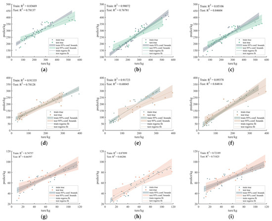
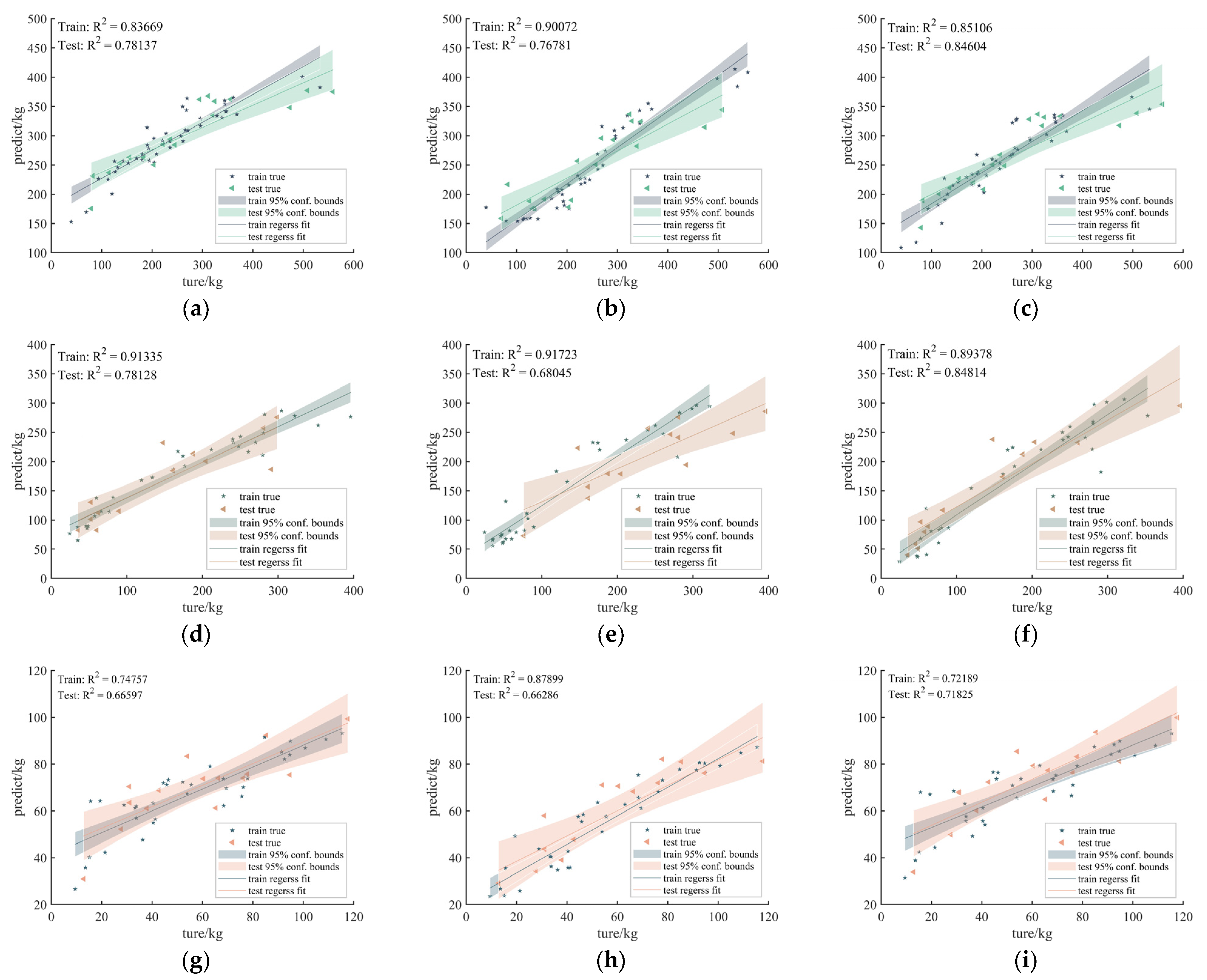
The results from MLR, RFR, and SVR consistently indicated that multi-feature fusion outperformed single-feature inputs across degradation states (Figure 5). In all three degradation states, SVR (R² = 0.846/0.848/0.718) (Figure 5c,f,i) achieved higher predictive accuracy than MLR (R² = 0.808/0.781/0.666) (Figure 5a,d,g) and RFR (R² = 0.720/0.695/0.663) (Figure 5b,e,h). Using both structural features and vegetation indices improved the test-set R² compared with using structural features or vegetation indices alone. In the healthy state, R² increased by 19.39% and 321.84%, while RMSE decreased by 7.78% and 62.83%. In the moderately degraded state, R² increased by 10.38% and 104.13%, while RMSE decreased by 21.71% and 52.18%. In the severely degraded state, R² increased by 69.51% and 574.20%, while RMSE decreased by 48.85% and 58.91%. These results support the utility of SVR for AGB estimation across degradation levels and highlight the benefit of integrating structural and spectral features.

Figure 5. Test-set accuracy comparison of multi-feature fusion AGB estimation models for farmland shelterbelts across degradation levels. Panels (a–c) show the fitted results for the healthy state using MLR, RFR, and SVR with fused structural features and vegetation indices; panels (d–f) show the fitted results for the moderately degraded state; and panels (g–i) show the fitted results for the severely degraded state. For all panels, models were trained on the training set and evaluated on the held-out test set using a stratified 70/30 split.

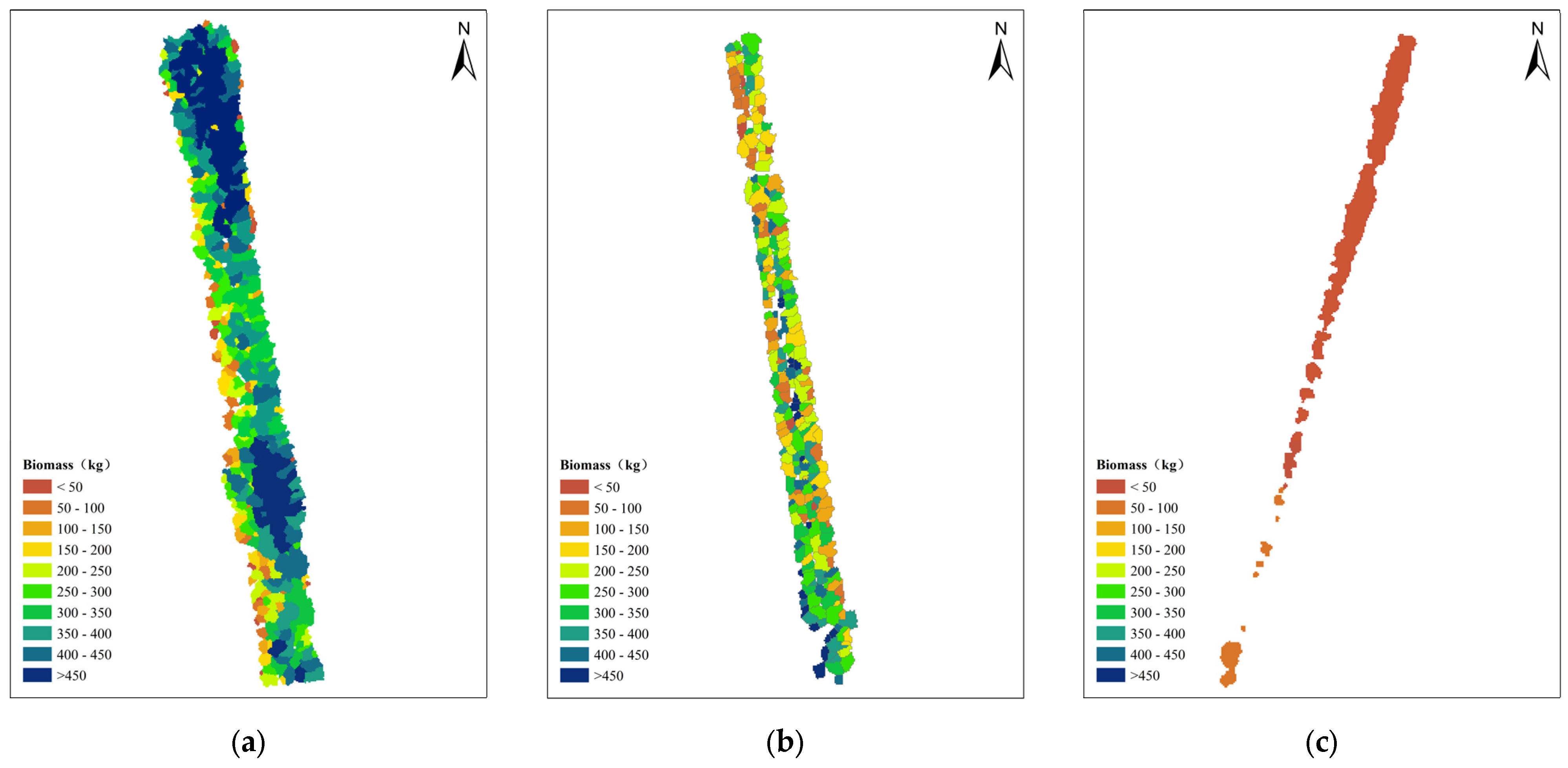
Using the SVR model trained with “structural features + vegetation indices” fusion data, the spatial distribution of individual tree AGB in shelterbelts with different degradation levels was mapped (Figure 6). In the healthy shelterbelt (Figure 6a), individual tree AGB is generally at a high level, with most points exceeding 200 kg. A low-value zone (<100 kg) is observed on the western side of the shelterbelt. In the moderately degraded shelterbelt (Figure 6b), clear patchy and interwoven distribution patterns are observed, with low, medium, and high biomass zones alternating within the shelterbelt, reflecting significant spatial heterogeneity of individual tree AGB. In the severely degraded shelterbelt (Figure 6c), AGB levels are generally low, consistent with the observed growth decline in the field investigation (e.g., localized dieback, branch dieback, and increased deadwood).

Figure 6. Distribution of AGB (aboveground biomass) of farmland shelterbelts in different degradation states based on SVR. (a) Healthy, (b) Moderately degraded, (c) Severely degraded.

3.4. Selection Criteria and Robustness Test of Scaling Correction Factor (ρ)

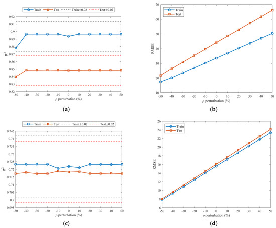
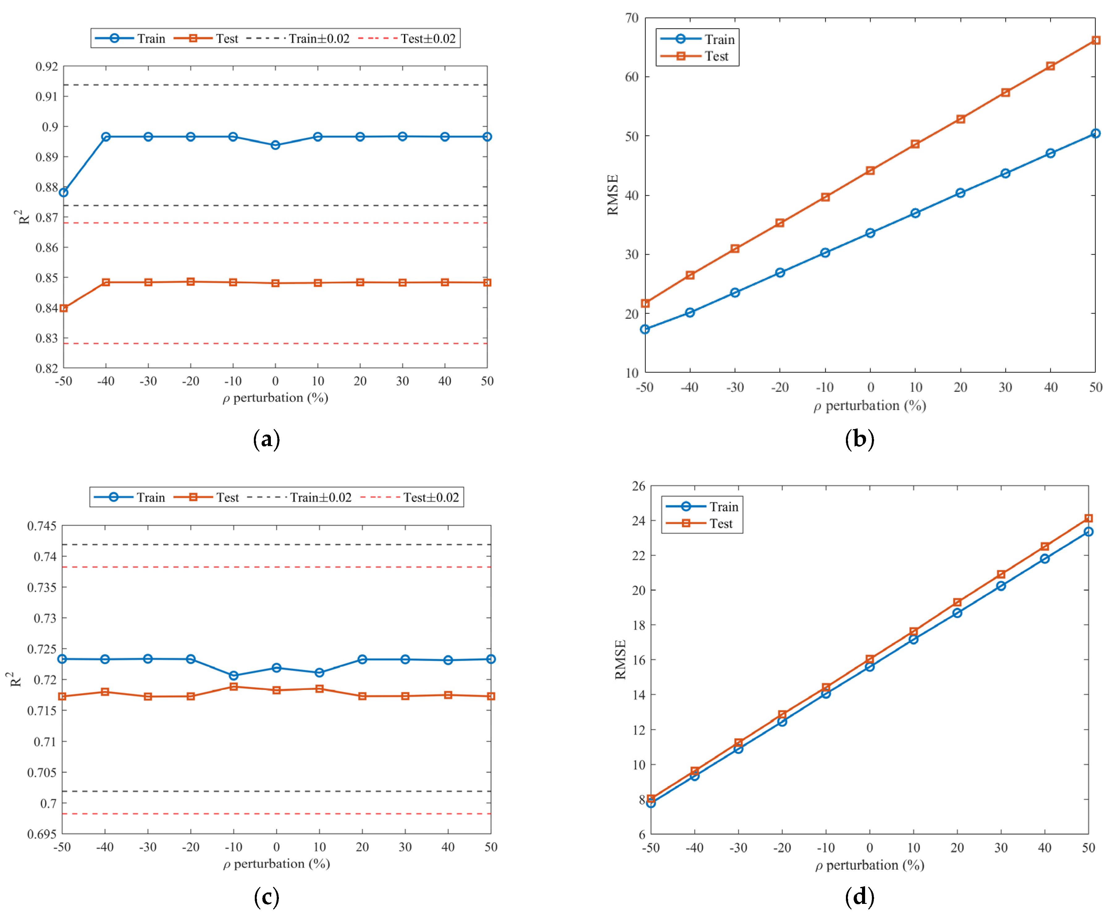
To test the reliability of the scale correction coefficient, we perturbed the baseline ρ by relative factors (1 ± 10%, 1 ± 20%, 1 ± 30%, and 1 ± 50%), i.e., ρ′ = ρ·(1 + δ) where δ ∈ {±0.1, ±0.2, ±0.3, ±0.5}. This sensitivity test modifies only the scaling of reference AGB while keeping model predictions fixed. The resulting variations in R2 and RMSE are shown in Figure 7.

Figure 7. Variations in R² and RMSE in the model under different ρ perturbations. (a) Variation in R² in the moderately degraded state; (b) Variation in RMSE in the moderately degraded state; (c) Variation in R² in the severely degraded state; (d) Variation in RMSE in the severely degraded state.

3.5. Contribution of Spectral and Structural Features to AGB Estimation of Farmland Shelterbelts with Different Degradation Levels

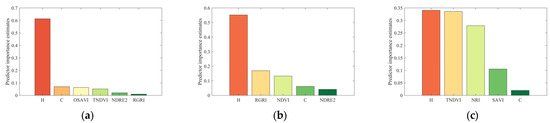
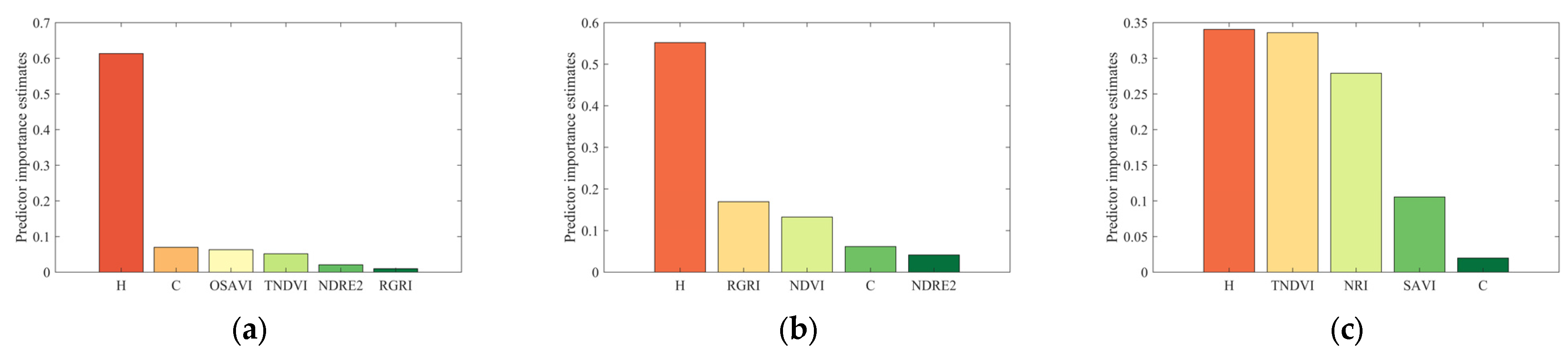
SHapley Additive exPlanations (SHAP) is a powerful tool for interpreting machine learning models, especially those considered “black-box” like deep neural networks or ensemble models. To deepen the understanding of how different features affect AGB estimation of farmland shelterbelts with varying degradation levels, SHAP was used to analyze the interpretability of the feature variables integrated in the SVR model. This analysis clarified the extent to which each feature value influences the model output under different degradation states (Figure 8). The results showed that in healthy farmland shelterbelts, tree height was significantly more important than crown width and vegetation indices, with higher importance associated with a more substantial positive impact on the model (Figure 8a). In contrast, vegetation indices play a crucial role in AGB estimation for severely degraded farmland shelterbelts, with their importance increasing and having a positive effect on the model output (Figure 8c), with TNDVI having the greatest impact. For both moderately and severely degraded stages, the synergistic effect of structural features and vegetation indices contributed significantly to AGB estimation, indicating that the inclusion of both feature types leads to a greater positive impact on the model output (Figure 8c). These results further support the SHAP-based interpretability analysis, highlighting the advantage of integrating structural features and vegetation indices for AGB estimation across degradation levels and suggesting that key vegetation indices should be selected adaptively according to degradation status.

Figure 8. Summary diagram of SHAP (SHapley Additive exPlanations) estimation models for AGB (aboveground biomass) of shelterbelts with different degradation levels based on SVR. (a) Healthy state, (b) Moderately degraded state, (c) Severely degraded state.

3.6. SHAP Dependence Analysis Reveals Differences in the Contributions of Key Factors Across Different Degradation Levels

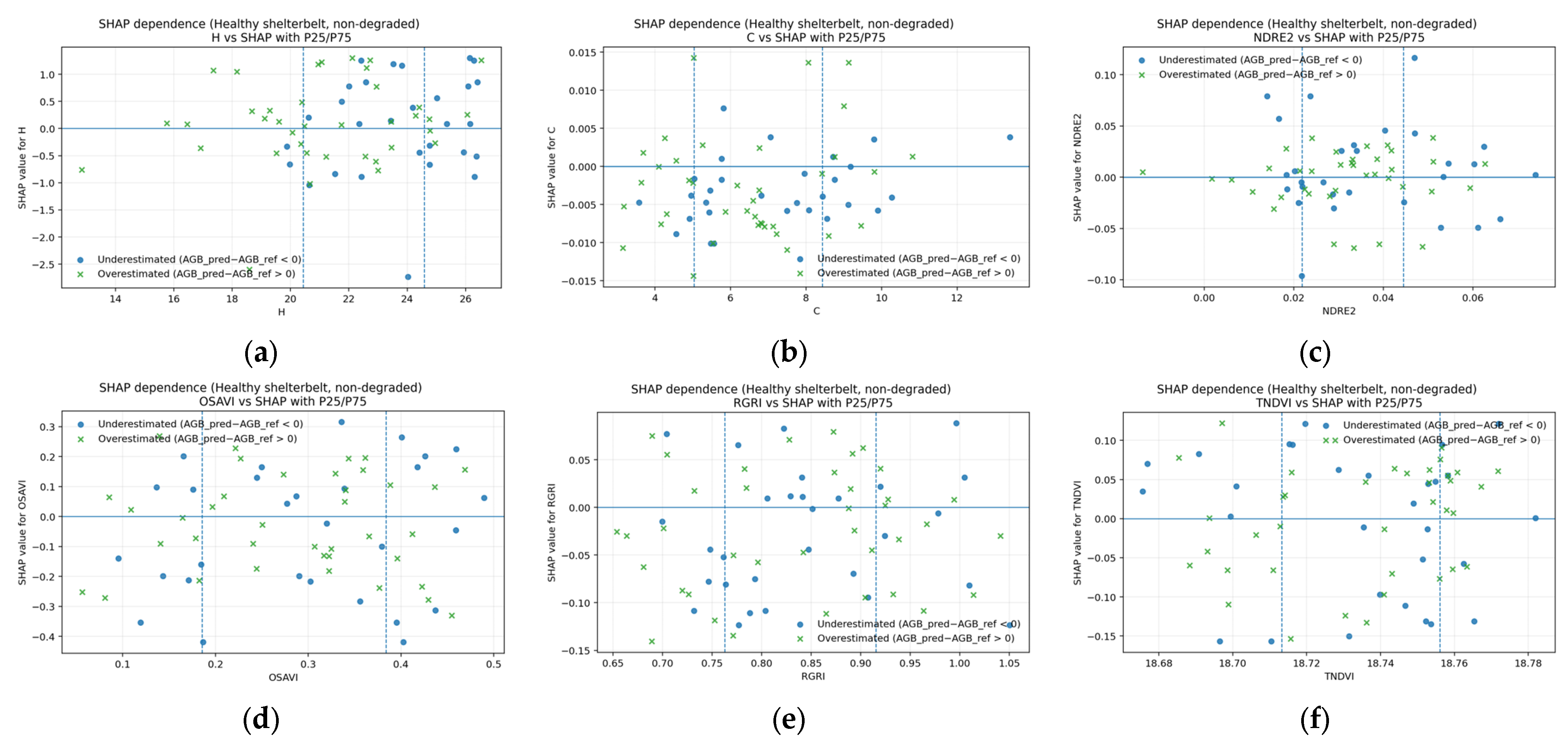
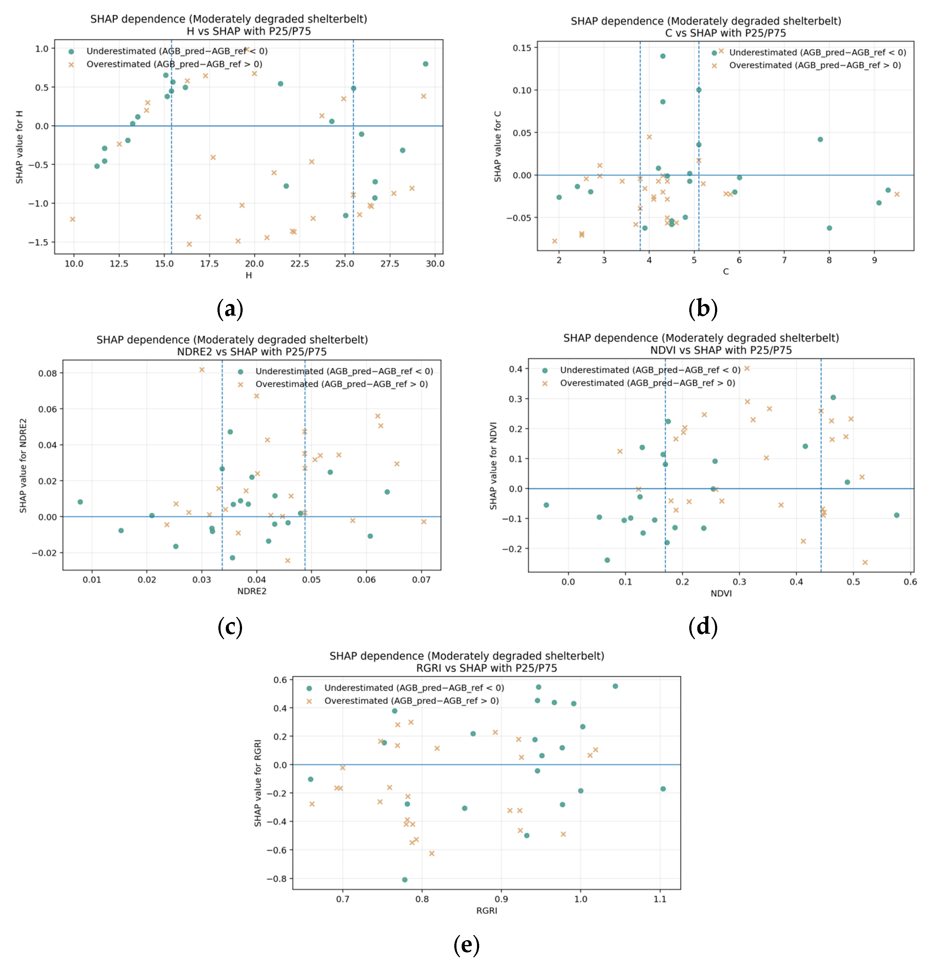
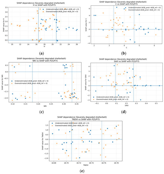
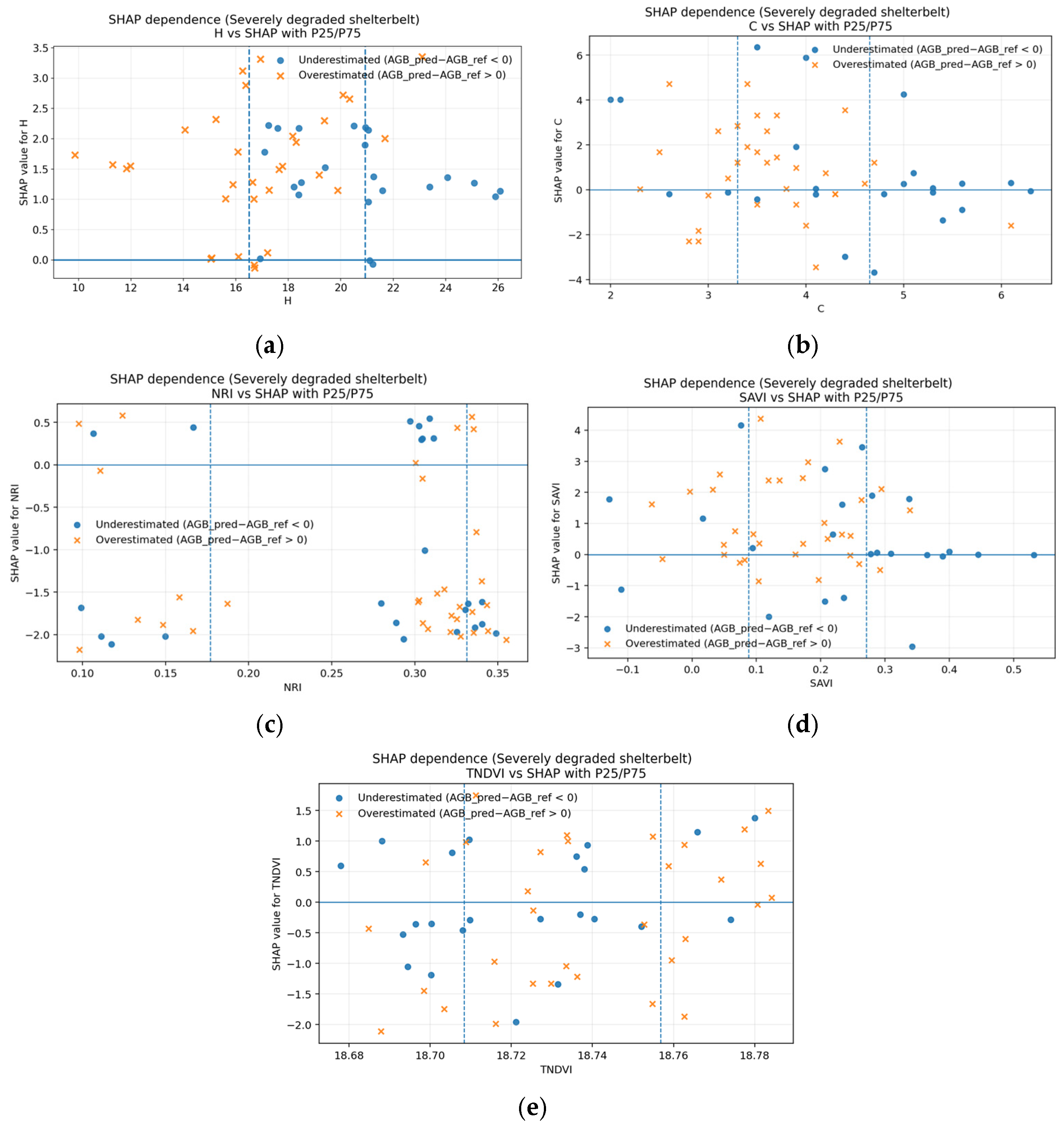
To further interpret the driving factors behind model predictions and how their effects vary across degradation levels, we plotted SHAP dependence plots for the healthy, moderately degraded, and severely degraded shelterbelts (Figure 9, Figure 10 and Figure 11). Samples were grouped as underestimation (AGB_pred − AGB_ref < 0) or overestimation (AGB_pred − AGB_ref > 0) based on the residual sign. For each key predictor, we examined the SHAP distributions across the lower quartile (<P25), the interquartile range (P25–P75), and the upper quartile (>P75) to highlight where prediction errors tended to accumulate.

Figure 9. SHAP dependence plots of key structural and spectral features for AGB prediction in the healthy shelterbelt.

Figure 10. SHAP dependence plots of key structural and spectral features for AGB prediction in the moderately degraded shelterbelt.

Figure 11. SHAP dependence plots of key structural and spectral features for AGB prediction in the severely degraded shelterbelt.

In the moderately degraded shelterbelt (Figure 10), SHAP values were more dispersed than in the healthy belt, especially for structural variables (H and C), indicating stronger interval sensitivity under transitional canopy conditions. Vegetation indices (e.g., NDVI, NDRE2, and RGRI) showed clearer sign shifts across value ranges, suggesting an increased reliance on canopy vitality signals to compensate for structural uncertainty. Under- and over-estimated samples tended to cluster more frequently toward the distribution tails (<P25 or >P75), implying that extreme structural or spectral conditions are associated with higher extrapolation risk.

In the severely degraded shelterbelt (Figure 11), both structural and spectral predictors exhibited stronger nonlinearity and larger fluctuations in SHAP contributions. The effects of H and C varied substantially across ranges, reflecting the weakened and less stable structure–biomass relationship under severe crown fragmentation. Meanwhile, spectral indices related to greenness and red-edge activity (e.g., SAVI/OSAVI, TNDVI, and NDRE2) showed more pronounced positive/negative contributions in specific intervals, highlighting their complementary role in correcting structural bias when degradation is severe.

Taken together (Figure 9, Figure 10 and Figure 11), the healthy belt shows relatively concentrated SHAP distributions and mixed error signs within the main range (P25–P75). The moderately degraded belt displays increased dispersion and stronger interval sensitivity, while the severely degraded belt presents the clearest nonlinearity: the contribution stability of structural variables (particularly crown width) declines, and spectral variables become more influential. These results suggest that, along the degradation gradient, biomass estimation increasingly depends on the combined state of “structure + vitality”, whereas a single structural or spectral predictor alone becomes insufficient to robustly explain AGB variation.

4. Discussion

4.1. The Impact of Scale Correction Factor (ρ) Perturbation on the Stability of AGB Inverted Structures

The scale correction factor ρ was introduced as a prior-constrained scaling coefficient to harmonize allometry-based reference AGB with field-derived geometric constraints (i.e., volumes inferred from measured D, height, and crown width) under a physically feasible domain defined by wood density [11,50,51,52], biomass expansion factor, and crown-shape coefficient [53,54,55,56,57]. This strategy followed the general rationale of using multiplicative correction factors in biomass estimation to reduce systematic bias caused by log–linear back-transformation and scale conversion [17,58,59]. In this study, ρ acted as a uniform scaling term applied to the nominal allometric AGB, enabling the reference values to remain physically plausible while avoiding overly confident point estimates.

Sensitivity analysis showed that moderate perturbations of ρ mainly affected absolute error metrics, whereas correlation-based metrics were relatively stable [60]. This behavior was expected because correlation is less sensitive to a global scaling change than absolute deviations [60,61,62]. Importantly, ρ should be interpreted as a theoretical consistency adjustment rather than a biologically verified correction, since destructive biomass measurements were not available [63,64,65,66]. Therefore, the reported model errors primarily reflected the ability to reproduce allometry-based reference AGB within the study system rather than the absolute error against true biomass.

4.2. Mechanism of Action and Synergistic Enhancement of Spectral−Structural Features

Across degradation levels, LiDAR structural metrics provided a stable baseline because tree height and crown width captured major variations in tree size [55,67,68]. However, under severe degradation, the relationship between geometry and biomass weakened due to crown fragmentation, branch dieback, internal hollowness, and increased canopy gaps [69,70]. In such cases, trees could retain comparable geometric dimensions while losing woody biomass and canopy vitality, which reduced the explanatory power of structural variables alone [17,71,72].

Multispectral vegetation indices, although often limited by saturation and background mixing, provided complementary sensitivity to canopy greenness, chlorophyll activity, and stress-related changes [21,73,74,75]. When fused with LiDAR structure, spectral information helped correct the bias arising from geometry–biomass decoupling in degraded belts, leading to a larger improvement under severe degradation than under healthy conditions [11,76,77]. This pattern supported the ecological interpretation that structure dominates when growth is healthy, whereas spectral vitality becomes increasingly informative when degradation disrupts structural–biomass coupling [78,79,80].

From an ecological perspective, soil-adjusted indices (e.g., SAVI/OSAVI) are more robust to exposed soil signals under sparse or fragmented canopies [20,39], whereas red-edge-related indices (e.g., NDRE) better track chlorophyll dynamics and stress responses [41,81], which tend to dominate as degradation intensifies. Therefore, the degradation-dependent importance of spectral predictors observed in Figure 3 and the SHAP analyses is consistent with expected shifts from ‘structure-driven’ to ‘vitality-driven’ biomass inference along the degradation gradient [82,83].

4.3. Performance Comparison of MLR, RFR, and SVR in AGB Estimation

When using the same fused feature set, the three algorithms exhibited distinct behavior [10,84,85]. The linear model (MLR) remained competitive in healthy and moderately degraded belts, suggesting that the dominant structure–AGB relationship still contained a strong linear component [10,86]. Random Forest did not consistently outperform the other methods, which was likely related to limited sample size and the tendency of ensemble trees to overfit local patterns when training data are sparse or highly heterogeneous [87,88]. In contrast, SVR showed the most stable performance under fusion inputs, indicating stronger robustness to nonlinear interactions and noise within the available sample space.

These findings suggested that algorithm selection should consider not only theoretical model flexibility but also sample size, predictor redundancy, and degradation-driven heterogeneity, all of which can influence generalization stability [87,89].

4.4. Explanation of the Complementary Mechanism and Error Sources of Structural and Spectral Information Under Degradation Gradient

SHAP dependence plots provided interpretable evidence that the importance of structural and spectral variables shifted along the degradation gradient. In the healthy belt, contributions from height and crown width were relatively concentrated, consistent with a stable geometric control on biomass [11,90]. With increasing degradation, the influence of vegetation indices became more pronounced, reflecting the rising importance of canopy vitality signals for correcting structural uncertainty.

A consistent practical pattern was that larger prediction errors tended to occur at the tails of predictor distributions rather than in the central range. This suggests an operational interpretation strategy based on a “structure + vitality” framework: segments with moderate-to-high structure but low spectral vitality may indicate emerging degradation and should be prioritized for field inspection, whereas segments with simultaneously low structure and low vitality are more likely candidates for renewal or replanting. It should be noted that SHAP reflects marginal contributions within the current sample space and does not imply strict causality, and thus these interpretation rules should be used as guidance rather than hard physical thresholds.

To address the notably higher relative error in the moderately degraded belt, a plausible explanation is that this class represented a transitional state with the strongest within-belt heterogeneity: trees with mixed vitality levels coexisted, canopy gaps were spatially intermittent, and background mixing effects were more variable than in the relatively homogeneous healthy belt [91,92]. Such heterogeneity can increase uncertainty in both spectral responses and structural segmentation, leading to a higher rRMSE even when overall correlation remains reasonable [66,93].

4.5. Limitations and Applicability

This study was conducted in a single region and a single acquisition campaign (October 2024) for one dominant species (Populus euphratica Olivier). Reference AGB was derived from nondestructive allometric equations with a prior-constrained scale correction factor, rather than destructively weighed biomass. Therefore, the reported performance quantified the internal consistency and relative predictive capability of UAV-derived features under the local allometric framework, and the absolute error against true biomass may be larger.

Future work should include replicated shelterbelts across multiple sites and seasons, cross-belt validation, and a limited number of destructively sampled trees to calibrate and verify absolute biomass. These steps are necessary to evaluate transferability and to confirm the biological reliability of the proposed framework for broader regional applications.

5. Conclusions

We present a non-destructive UAV-based workflow for estimating individual-tree AGB of farmland shelterbelts across degradation levels by combining LiDAR-derived structural metrics with multispectral vegetation indices. Because destructive harvesting is infeasible in operational shelterbelts, we used allometry-derived AGB as the reference AGB (AGB_ref), and introduced a prior-constrained scale coefficient (ρ) to maintain physical plausibility under a non-destructive regime. Therefore, the reported model performance should be interpreted as agreement with AGB_ref rather than absolute accuracy against destructively measured biomass.

Across degradation classes, feature fusion consistently improved test-set performance relative to single-source inputs. LiDAR structural metrics provided a strong baseline under healthy to moderately degraded conditions, whereas multispectral indices became increasingly informative under severe degradation, consistent with intensified canopy fragmentation and background mixing that weaken geometry–biomass coupling. Among the tested algorithms, the fused SVR achieved the highest overall agreement with AGB_ref, supporting the complementarity of structural and spectral cues for characterizing degraded shelterbelts.

Despite the methodological generality of the workflow, this study represents a single-site, single-season, single-species case study, and the fitted parameters (including ρ and model weights) are expected to be site- and condition-dependent. The scale coefficient ρ should be interpreted as a theoretical consistency adjustment rather than a biologically verified correction.

Future work should prioritize (i) multi-site and multi-season evaluations with independent validation belts and (ii) independent biomass measurements (where feasible) to quantify absolute error and improve model transferability.

References

- Brandle, J.R.; Hodges, L.; Zhou, X.H. Windbreaks in North American agricultural systems. Agrofor. Syst. 2004, 61, 65–78. [Google Scholar] [CrossRef] [Scilit]
- Mize, C.; Brandle, J.R.; Schoeneberger, M.; Bentrup, G. Ecological development and function of shelterbelts in temperate North America. In Toward Agroforestry Design: An Ecological Approach; Springer: Dordrecht, The Netherlands, 2008; pp. 27–54. [Google Scholar]
- Kort, J. 9. Benefits of windbreaks to field and forage crops. Agric. Ecosyst. Environ. 1988, 22, 165–190. [Google Scholar] [CrossRef] [Scilit]
- Zheng, X.; Zhu, J.; Xing, Z. Assessment of the effects of shelterbelts on crop yields at the regional scale in Northeast China. Agric. Syst. 2016, 143, 49–60. [Google Scholar] [CrossRef] [Scilit]
- Wang, X.; Zhang, C.; Hasi, E.; Dong, Z. Has the Three Norths Forest Shelterbelt Program solved the desertification and dust storm problems in arid and semiarid China? J. Arid Environ. 2010, 74, 13–22. [Google Scholar] [CrossRef] [Scilit]
- Ahrends, A.; Hollingsworth, P.M.; Beckschäfer, P.; Chen, H.; Zomer, R.J.; Zhang, L.; Wang, M.; Xu, J. China’s fight to halt tree cover loss. Proc. R. Soc. B Biol. Sci. 2017, 284, 20162559. [Google Scholar] [CrossRef] [Scilit]
- Stone, R. Nursing China’s Ailing Forests Back to Health. Science 2009, 325, 556–558. [Google Scholar] [CrossRef] [Scilit]
- Lechner, A.M.; Stein, A.; Jones, S.D.; Ferwerda, J.G. Remote sensing of small and linear features: Quantifying the effects of patch size and length, grid position and detectability on land cover mapping. Remote Sens. Environ. 2009, 113, 2194–2204. [Google Scholar] [CrossRef] [Scilit]
- Wang, J.; Patruno, L.; Zhao, G.; Tamura, Y. Windbreak effectiveness of shelterbelts with different characteristic parameters and arrangements by means of CFD simulation. Agric. For. Meteorol. 2024, 344, 109813. [Google Scholar] [CrossRef] [Scilit]
- Lu, D.; Chen, Q.; Wang, G.; Liu, L.; Li, G.; Moran, E. A survey of remote sensing-based aboveground biomass estimation methods in forest ecosystems. Int. J. Digit. Earth 2016, 9, 63–105. [Google Scholar] [CrossRef] [Scilit]
- Zolkos, S.G.; Goetz, S.J.; Dubayah, R. A meta-analysis of terrestrial aboveground biomass estimation using lidar remote sensing. Remote Sens. Environ. 2013, 128, 289–298. [Google Scholar] [CrossRef] [Scilit]
- HAO, Q.; HUANG, C. A review of forest aboveground biomass estimation based on remote sensing data. Chin. J. Plant Ecol. 2023, 47, 1356. [Google Scholar] [CrossRef] [Scilit]
- Fu, S.; Sun, L.; Luo, Y. Canopy conductance and stand transpiration of Populus simonii Carr in response to soil and atmospheric water deficits in farmland shelterbelt, Northwest China. Agrofor. Syst. 2017, 91, 1165–1180. [Google Scholar] [CrossRef] [Scilit]
- Lefsky, M.A.; Cohen, W.B.; Harding, D.J.; Parker, G.G.; Acker, S.A.; Gower, S.T. Lidar remote sensing of above-ground biomass in three biomes. Glob. Ecol. Biogeogr. 2002, 11, 393–399. [Google Scholar] [CrossRef] [Scilit]
- Gleason, C.J.; Im, J. Forest biomass estimation from airborne LiDAR data using machine learning approaches. Remote Sens. Environ. 2012, 125, 80–91. [Google Scholar] [CrossRef] [Scilit]
- Sprugel, D.G. Correcting for bias in log-transformed allometric equations. Ecology 1983, 64, 209–210. [Google Scholar] [CrossRef] [Scilit]
- Baskerville, G. Use of logarithmic regression in the estimation of plant biomass. Can. J. For. Res. 1972, 2, 49–53. [Google Scholar] [CrossRef] [Scilit]
- Dandois, J.P.; Ellis, E.C. High spatial resolution three-dimensional mapping of vegetation spectral dynamics using computer vision. Remote Sens. Environ. 2013, 136, 259–276. [Google Scholar] [CrossRef] [Scilit]
- Adão, T.; Hruška, J.; Pádua, L.; Bessa, J.; Peres, E.; Morais, R.; Sousa, J.J. Hyperspectral imaging: A review on UAV-based sensors, data processing and applications for agriculture and forestry. Remote Sens. 2017, 9, 1110. [Google Scholar] [CrossRef] [Scilit]
- Rondeaux, G.; Steven, M.; Baret, F. Optimization of soil-adjusted vegetation indices. Remote Sens. Environ. 1996, 55, 95–107. [Google Scholar] [CrossRef] [Scilit]
- Huete, A.; Didan, K.; Miura, T.; Rodriguez, E.P.; Gao, X.; Ferreira, L.G. Overview of the radiometric and biophysical performance of the MODIS vegetation indices. Remote Sens. Environ. 2002, 83, 195–213. [Google Scholar] [CrossRef] [Scilit]
- Badgley, G.; Field, C.; Berry, J. Canopy near-infrared reflectance and terrestrial photosynthesis. Sci. Adv. 2017, 3, e1602244. [Google Scholar] [CrossRef] [Scilit]
- Asner, G.P.; Powell, G.V.; Mascaro, J.; Knapp, D.E.; Clark, J.K.; Jacobson, J.; Kennedy-Bowdoin, T.; Balaji, A.; Paez-Acosta, G.; Victoria, E. High-resolution forest carbon stocks and emissions in the Amazon. Proc. Natl. Acad. Sci. USA 2010, 107, 16738–16742. [Google Scholar] [CrossRef] [Scilit]
- Asner, G.P.; Hughes, R.F.; Mascaro, J.; Uowolo, A.L.; Knapp, D.E.; Jacobson, J.; Kennedy-Bowdoin, T.; Clark, J.K. High-resolution carbon mapping on the million-hectare Island of Hawaii. Front. Ecol. Environ. 2011, 9, 434–439. [Google Scholar] [CrossRef] [Scilit]
- Fernández-Guisuraga, J.M.; Suárez-Seoane, S.; Fernandes, P.M.; Fernández-García, V.; Fernández-Manso, A.; Quintano, C.; Calvo, L. Pre-fire aboveground biomass, estimated from LiDAR, spectral and field inventory data, as a major driver of burn severity in maritime pine (Pinus pinaster) ecosystems. For. Ecosyst. 2022, 9, 100022. [Google Scholar] [CrossRef] [Scilit]
- GB/T 44351-2024; Code of Practice for Degraded Forest Remediation and Restoration. Standardization Administration of China: Beijing, China, 2024.
- Penman, J.; Gytarsky, M.; Hiraishi, T.; Krug, T.; Kruger, D.; Pipatti, R.; Buendia, L.; Miwa, K.; Ngara, T.; Tanabe, K. Good Practice Guidance for Land Use, Land-Use Change and Forestry; Institute for Global Environmental Strategies (IGES): Hayama, Japan, 2003. [Google Scholar]
- Eggleston, H.; Buendia, L.; Miwa, K.; Ngara, T.; Tanabe, K. 2006 IPCC Guidelines for National Greenhouse Gas Inventories; Institute for Global Environmental Strategies (IGES): Hayama, Japan, 2006. [Google Scholar]
- Erfanifard, Y.; Stereńczak, K.; Kraszewski, B.; Kamińska, A. Development of a robust canopy height model derived from ALS point clouds for predicting individual crown attributes at the species level. Int. J. Remote Sens. 2018, 39, 9206–9227. [Google Scholar] [CrossRef] [Scilit]
- Zhou, X.; Ma, K.; Sun, H.; Li, C.; Wang, Y. Estimation of forest stand volume in coniferous plantation from individual tree segmentation aspect using UAV-LiDAR. Remote Sens. 2024, 16, 2736. [Google Scholar] [CrossRef] [Scilit]
- Gitelson, A.A.; Viña, A.; Arkebauer, T.J.; Rundquist, D.C.; Keydan, G.; Leavitt, B. Remote estimation of leaf area index and green leaf biomass in maize canopies. Geophys. Res. Lett. 2003, 30, 1248. [Google Scholar] [CrossRef] [Scilit]
- Biró, L.; Kozma-Bognár, V.; Berke, J. Comparison of RGB Indices used for Vegetation Studies based on Structured Similarity Index (SSIM). J. Plant Sci. Phytopathol. 2024, 8, 7–12. [Google Scholar] [CrossRef] [Scilit]
- Jiang, Z.; Huete, A.R.; Didan, K.; Miura, T. Development of a two-band enhanced vegetation index without a blue band. Remote Sens. Environ. 2008, 112, 3833–3845. [Google Scholar] [CrossRef] [Scilit]
- Woebbecke, D.M.; Meyer, G.E.; Von Bargen, K.; Mortensen, D.A. Color indices for weed identification under various soil, residue, and lighting conditions. Trans. ASAE 1995, 38, 259–269. [Google Scholar] [CrossRef] [Scilit]
- Meyer, G.E.; Neto, J.C. Verification of color vegetation indices for automated crop imaging applications. Comput. Electron. Agric. 2008, 63, 282–293. [Google Scholar] [CrossRef] [Scilit]
- Mao, X.; Deng, Y.; Zhu, L.; Yao, Y. Hierarchical geographic object-based vegetation type extraction based on multi-source remote sensing data. Forests 2020, 11, 1271. [Google Scholar] [CrossRef] [Scilit]
- Datt, B. A new reflectance index for remote sensing of chlorophyll content in higher plants: Tests using Eucalyptus leaves. J. Plant Physiol. 1999, 154, 30–36. [Google Scholar] [CrossRef] [Scilit]
- Bendig, J.; Yu, K.; Aasen, H.; Bolten, A.; Bennertz, S.; Broscheit, J.; Gnyp, M.L.; Bareth, G. Combining UAV-based plant height from crop surface models, visible, and near infrared vegetation indices for biomass monitoring in barley. Int. J. Appl. Earth Obs. Geoinf. 2015, 39, 79–87. [Google Scholar] [CrossRef] [Scilit]
- Qi, J.; Chehbouni, A.; Huete, A.R.; Kerr, Y.H.; Sorooshian, S. A modified soil adjusted vegetation index. Remote Sens. Environ. 1994, 48, 119–126. [Google Scholar] [CrossRef] [Scilit]
- Torino, M.S.; Ortiz, B.V.; Fulton, J.P.; Balkcom, K.S.; Wood, C.W. Evaluation of vegetation indices for early assessment of corn status and yield potential in the southeastern United States. Agron. J. 2014, 106, 1389–1401. [Google Scholar] [CrossRef] [Scilit]
- Clevers, J.G.; Gitelson, A.A. Remote estimation of crop and grass chlorophyll and nitrogen content using red-edge bands on Sentinel-2 and-3. Int. J. Appl. Earth Obs. Geoinf. 2013, 23, 344–351. [Google Scholar] [CrossRef] [Scilit]
- Rous, J.W., Jr.; Haas, R.H.; Schell, J.; Deering, D. Monitoring the Vernal Advancement and Retrogradation (Green Wave Effect) of Natural Vegetation; National Aeronautics and Space Administration: Washington, DC, USA, 1973.
- Richardson, A.D.; Hufkens, K.; Milliman, T.; Aubrecht, D.M.; Chen, M.; Gray, J.M.; Johnston, M.R.; Keenan, T.F.; Klosterman, S.T.; Kosmala, M. Tracking vegetation phenology across diverse North American biomes using PhenoCam imagery. Sci. Data 2018, 5, 180028. [Google Scholar] [CrossRef] [Scilit]
- Hunt, E.R., Jr.; Cavigelli, M.; Daughtry, C.S.; Mcmurtrey, J.E., III; Walthall, C.L. Evaluation of digital photography from model aircraft for remote sensing of crop biomass and nitrogen status. Precis. Agric. 2005, 6, 359–378. [Google Scholar] [CrossRef] [Scilit]
- Jiang, J.; Cai, W.; Zheng, H.; Cheng, T.; Tian, Y.; Zhu, Y.; Ehsani, R.; Hu, Y.; Niu, Q.; Gui, L. Using digital cameras on an unmanned aerial vehicle to derive optimum color vegetation indices for leaf nitrogen concentration monitoring in winter wheat. Remote Sens. 2019, 11, 2667. [Google Scholar] [CrossRef] [Scilit]
- Huete, A.R. A soil-adjusted vegetation index (SAVI). Remote Sens. Environ. 1988, 25, 295–309. [Google Scholar] [CrossRef] [Scilit]
- Jordan, C.F. Derivation of leaf-area index from quality of light on the forest floor. Ecology 1969, 50, 663–666. [Google Scholar] [CrossRef] [Scilit]
- Dering, D.W. Measuring forage production of grazing units from Landsat MSS data. In Proceedings of the 10th International Symposium on Remote Sensing of Environment, Ann Arbor, MI, USA, 15–19 April 1974; pp. 1169–1178. [Google Scholar]
- Xiaoqin, W.; Miaomiao, W.; Shaoqiang, W.; Yundong, W. Extraction of vegetation information from visible unmanned aerial vehicle images. Trans. Chin. Soc. Agric. Eng. 2015, 31, 152. [Google Scholar]
- Duncanson, L.; Armston, J.; Disney, M.; Avitabile, V.; Barbier, N.; Calders, K.; Carter, S.; Chave, J.; Herold, M.; MacBean, N. Aboveground Woody Biomass Product Validation Good Practices Protocol; Committee on Earth Observation Satellites Working Group on Calibration and Validation, Land Product Validation Subgroup: Greenbelt, MD, USA, 2021.
- Chave, J.; Andalo, C.; Brown, S.; Cairns, M.A.; Chambers, J.Q.; Eamus, D.; Fölster, H.; Fromard, F.; Higuchi, N.; Kira, T. Tree allometry and improved estimation of carbon stocks and balance in tropical forests. Oecologia 2005, 145, 87–99. [Google Scholar] [CrossRef] [Scilit]
- Lim, K.; Treitz, P.; Wulder, M.; St-Onge, B.; Flood, M. LiDAR remote sensing of forest structure. Prog. Phys. Geogr. 2003, 27, 88–106. [Google Scholar] [CrossRef] [Scilit]
- Picard, N.; Saint-André, L.; Henry, M. Manual for Building Tree Volume and Biomass Allometric Equations: From Field Measurement to Prediction; FAO: Rome, Italy, 2012. [Google Scholar]
- Chave, J.; Réjou-Méchain, M.; Búrquez, A.; Chidumayo, E.; Colgan, M.S.; Delitti, W.B.; Duque, A.; Eid, T.; Fearnside, P.M.; Goodman, R.C. Improved allometric models to estimate the aboveground biomass of tropical trees. Glob. Change Biol. 2014, 20, 3177–3190. [Google Scholar] [CrossRef] [Scilit]
- Næsset, E. Predicting forest stand characteristics with airborne scanning laser using a practical two-stage procedure and field data. Remote Sens. Environ. 2002, 80, 88–99. [Google Scholar] [CrossRef] [Scilit]
- Lefsky, M.A.; Cohen, W.B.; Parker Geoffrey, G.; Harding, D.J. Lidar Remote Sensing for Ecosystem Studies. BioScience 2002, 52, 19–32. [Google Scholar] [CrossRef] [Scilit]
- Næsset, E. Accuracy of forest inventory using airborne laser scanning: Evaluating the first Nordic full-scale operational project. Scand. J. For. Res. 2004, 19, 554–557. [Google Scholar] [CrossRef] [Scilit]
- Clifford, D.; Cressie, N.; England, J.R.; Roxburgh, S.H.; Paul, K.I. Correction factors for unbiased, efficient estimation and prediction of biomass from log–log allometric models. For. Ecol. Manag. 2013, 310, 375–381. [Google Scholar] [CrossRef] [Scilit]
- Snowdon, P. A ratio estimator for bias correction in logarithmic regressions. Can. J. For. Res. 1991, 21, 720–724. [Google Scholar] [CrossRef] [Scilit]
- Akoglu, H. User’s guide to correlation coefficients. Turk. J. Emerg. Med. 2018, 18, 91–93. [Google Scholar] [CrossRef] [Scilit]
- Lee Rodgers, J.; Nicewander, W.A. Thirteen ways to look at the correlation coefficient. Am. Stat. 1988, 42, 59–66. [Google Scholar] [CrossRef] [Scilit]
- Cohen, J. Statistical Power Analysis for the Behavioral Sciences; Routledge: London, UK, 2013. [Google Scholar]
- Clark, D.A. Are tropical forests an important carbon sink? Reanalysis of the long-term plot data. Ecol. Appl. 2002, 12, 3–7. [Google Scholar] [CrossRef]
- Chave, J.; Chust, G.; Condit, R.; Aguilar, S.; Perez, R.; Lao, S. Error propagation and scaling for tropical forest biomass estimates. Philos Trans R Soc Lond B Biol Sci. 2004, 1443, 409–420. [Google Scholar] [CrossRef] [Scilit] [PubMed]
- Xu, Q.; Man, A.; Fredrickson, M.; Hou, Z.; Pitkänen, J.; Wing, B.; Ramirez, C.; Li, B.; Greenberg, J.A. Quantification of uncertainty in aboveground biomass estimates derived from small-footprint airborne LiDAR. Remote Sens. Environ. 2018, 216, 514–528. [Google Scholar] [CrossRef] [Scilit]
- Chen, Q.; Laurin, G.V.; Valentini, R. Uncertainty of remotely sensed aboveground biomass over an African tropical forest: Propagating errors from trees to plots to pixels. Remote Sens. Environ. 2015, 160, 134–143. [Google Scholar] [CrossRef] [Scilit]
- Malek, S.; Miglietta, F.; Gobakken, T.; Næsset, E.; Gianelle, D.; Dalponte, M. Prediction of stem diameter and biomass at individual tree crown level with advanced machine learning techniques. iForest-Biogeosci. For. 2019, 12, 323. [Google Scholar] [CrossRef] [Scilit]
- Means, J.E.; Acker, S.A.; Harding, D.J.; Blair, J.B.; Lefsky, M.A.; Cohen, W.B.; Harmon, M.E.; McKee, W.A. Use of large-footprint scanning airborne lidar to estimate forest stand characteristics in the Western Cascades of Oregon. Remote Sens. Environ. 1999, 67, 298–308. [Google Scholar] [CrossRef] [Scilit]
- Swatantran, A.; Dubayah, R.; Roberts, D.; Hofton, M.; Blair, J.B. Mapping biomass and stress in the Sierra Nevada using lidar and hyperspectral data fusion. Remote Sens. Environ. 2011, 115, 2917–2930. [Google Scholar] [CrossRef] [Scilit]
- Zheng, Z.; Zhang, S.; Baskin, C.; Baskin, J.; Schaefer, D.; Yang, X.; Yang, L. Hollows in living trees develop slowly but considerably influence the estimate of forest biomass. Funct. Ecol. 2016, 30, 830–838. [Google Scholar] [CrossRef] [Scilit]
- Asner, G.P.; Martin, R.E. Spectral and chemical analysis of tropical forests: Scaling from leaf to canopy levels. Remote Sens. Environ. 2008, 112, 3958–3970. [Google Scholar] [CrossRef] [Scilit]
- Asner, G.P.; Martin, R.E.; Anderson, C.B.; Knapp, D.E. Quantifying forest canopy traits: Imaging spectroscopy versus field survey. Remote Sens. Environ. 2015, 158, 15–27. [Google Scholar] [CrossRef] [Scilit]
- Baret, F.; Guyot, G. Potentials and limits of vegetation indices for LAI and APAR assessment. Remote Sens. Environ. 1991, 35, 161–173. [Google Scholar] [CrossRef] [Scilit]
- Carlson, T.N.; Ripley, D.A. On the relation between NDVI, fractional vegetation cover, and leaf area index. Remote Sens. Environ. 1997, 62, 241–252. [Google Scholar] [CrossRef] [Scilit]
- Sims, D.A.; Gamon, J.A. Relationships between leaf pigment content and spectral reflectance across a wide range of species, leaf structures and developmental stages. Remote Sens. Environ. 2002, 81, 337–354. [Google Scholar] [CrossRef] [Scilit]
- Balestra, M.; Marselis, S.; Sankey, T.T.; Cabo, C.; Liang, X.; Mokroš, M.; Peng, X.; Singh, A.; Stereńczak, K.; Vega, C. LiDAR data fusion to improve forest attribute estimates: A review. Curr. For. Rep. 2024, 10, 281–297. [Google Scholar] [CrossRef] [Scilit]
- Chen, A.; Wang, X.; Zhang, M.; Guo, J.; Xing, X.; Yang, D.; Zhang, H.; Hou, Z.; Jia, Z.; Yang, X. Fusion of LiDAR and multispectral data for aboveground biomass estimation in Mountain Grassland. Remote Sens. 2023, 15, 405. [Google Scholar] [CrossRef] [Scilit]
- Feng, Z.; Yang, Z.; Suo, L.; Wu, K.; Ma, Z.; Zhang, H.; Duan, J.; Feng, W. Enhancing maize above-ground biomass estimation through multispectral, digital and LiDAR fusion on UAV platforms. Agric. Water Manag. 2025, 315, 109551. [Google Scholar] [CrossRef] [Scilit]
- Kaviani, M.; Leblon, B.; Akilan, T.; Amishev, D.; LaRocque, A.; Haddadi, A. Tree Health Assessment Using Mask R-CNN on UAV Multispectral Imagery over Apple Orchards. Remote Sens. 2025, 17, 3369. [Google Scholar] [CrossRef] [Scilit]
- Pontius, J. A new approach for forest decline assessments: Maximizing detail and accuracy with multispectral imagery. Int. J. Remote Sens. 2014, 35, 3384–3402. [Google Scholar] [CrossRef] [Scilit]
- Dash, J.; Curran, P.J. MTCI: The MERIS terrestrial chlorophyll index. Int. J. Remote Sens 2004, 25, 151–161. [Google Scholar] [CrossRef] [Scilit]
- Goetz, S.; Dubayah, R. Advances in remote sensing technology and implications for measuring and monitoring forest carbon stocks and change. Carbon Manag. 2011, 2, 231–244. [Google Scholar] [CrossRef] [Scilit]
- Asner, G.P.; Knapp, D.E.; Kennedy-Bowdoin, T.; Jones, M.O.; Martin, R.E.; Boardman, J.W.; Field, C.B. Carnegie airborne observatory: In-flight fusion of hyperspectral imaging and waveform light detection and ranging for three-dimensional studies of ecosystems. J. Appl. Remote Sens. 2007, 1, 013536. [Google Scholar] [CrossRef] [Scilit]
- Thapa, N.; Narine, L.L.; Wilson, A.E. Forest Aboveground Biomass Estimation Using Airborne LiDAR: A Systematic Review and Meta-Analysis. J. For. 2025, 123, 389–421. [Google Scholar] [CrossRef] [Scilit]
- Belgiu, M.; Drăguţ, L. Random forest in remote sensing: A review of applications and future directions. ISPRS J. Photogramm. Remote Sens. 2016, 114, 24–31. [Google Scholar] [CrossRef] [Scilit]
- Zhang, Y.; Ma, J.; Liang, S.; Li, X.; Li, M. An evaluation of eight machine learning regression algorithms for forest aboveground biomass estimation from multiple satellite data products. Remote Sens. 2020, 12, 4015. [Google Scholar] [CrossRef] [Scilit]
- Cosenza, D.N.; Saarela, S.; Strunk, J.; Korhonen, L.; Maltamo, M.; Packalen, P. Effects of model-overfit on model-assisted forest inventory in boreal forests with remote sensing data. For. Int. J. For. Res. 2025, 98, 507–521. [Google Scholar] [CrossRef] [Scilit]
- Dormann, C.F.; Elith, J.; Bacher, S.; Buchmann, C.; Carl, G.; Carré, G.; Marquéz, J.R.G.; Gruber, B.; Lafourcade, B.; Leitão, P.J. Collinearity: A review of methods to deal with it and a simulation study evaluating their performance. Ecography 2013, 36, 27–46. [Google Scholar] [CrossRef] [Scilit]
- Gu, Y.; Wylie, B.K.; Boyte, S.P.; Picotte, J.; Howard, D.M.; Smith, K.; Nelson, K.J. An optimal sample data usage strategy to minimize overfitting and underfitting effects in regression tree models based on remotely-sensed data. Remote Sens. 2016, 8, 943. [Google Scholar] [CrossRef] [Scilit]
- Goodman, R.C.; Phillips, O.L.; del Castillo Torres, D.; Freitas, L.; Cortese, S.T.; Monteagudo, A.; Baker, T.R. Amazon palm biomass and allometry. For. Ecol. Manag. 2013, 310, 994–1004. [Google Scholar] [CrossRef] [Scilit]
- Asner, G.P. Biophysical and biochemical sources of variability in canopy reflectance. Remote Sens. Environ. 1998, 64, 234–253. [Google Scholar] [CrossRef] [Scilit]
- Turner, M.G. Landscape ecology: The effect of pattern on process. Annu. Rev. Ecol. Syst. 1989, 20, 171–197. [Google Scholar] [CrossRef]
- Mascaro, J.; Detto, M.; Asner, G.P.; Muller-Landau, H.C. Evaluating uncertainty in mapping forest carbon with airborne LiDAR. Remote Sens. Environ. 2011, 115, 3770–3774. [Google Scholar] [CrossRef] [Scilit]
Disclaimer/Publisher’s Note: The statements, opinions and data contained in all publications are solely those of the individual author(s) and contributor(s) and not of MDPI and/or the editor(s). MDPI and/or the editor(s) disclaim responsibility for any injury to people or property resulting from any ideas, methods, instructions or products referred to in the content. |
© 2026 by the authors. Licensee MDPI, Basel, Switzerland. This article is an open access article distributed under the terms and conditions of the Creative Commons Attribution (CC BY) license.