Analysis of Long-Memory GARCH-Type Model on Stock Returns and Setting Limits for Relative Risk Measures ^†

Abstract

The purpose of the article is to investigate whether considering stylized facts in financial time series leads to better estimation of risk measures. The study focuses on long-memory GARCH-type models chosen for their ability to capture characteristics of financial time series like long memory and volatility clustering. There are periods of high and low volatility in financial markets. One of the most important ways to reduce risk is to use a time-series model to manage market risk. In comparison to long-memory GARCH-type models, such as the fractionally integrated generalized autoregressive conditional heteroskedasticity, the research study aims to determine how effective the fractionally integrated asymmetric power autoregressive conditional heteroskedasticity is at producing competitive risk measures. The stock returns are assumed to follow an empirical and skewed Student-t distributions in long-memory GARCH-type models. The historical adjusted closing price time series for trading positions at the 95% and 99% confidence levels correspond to the quantiles of the empirical return distributions. Empirical results demonstrate that the FIGARCH model utilizing an empirical distribution significantly outperforms the presumptive skewed Student-t distribution in generating reliable risk measures.

1. Introduction

Understanding the relationship between risk measurement techniques and the statistical properties of financial time series is essential for selecting appropriate models that accurately capture market dynamics and improve forecasting and risk management performance. According to Kim and Shin [1], existing continuous-time volatility models fail to simultaneously capture key stylized facts of financial time series, such as persistence, volatility clustering, leverage effects and heavy-tailed distributions. This highlights the need to investigate whether accounting for the stylized facts of the stock price returns leads to better estimation of risk measures such as value at risk (VaR) and Expected Shortfall (ES) and their risk limits, focusing on long-memory GARCH-type models. Accurate quantification of financial market risk is important to portfolio management, regulatory capital adequacy and prudential supervision. VaR and ES have become the two dominant risk measures used by financial institutions and regulators, with ES formally adopted with the Basel Committee’s Fundamental Review of the Trading Book (FRTB) as the primary measure for internal models’ capital calculation [2]. This is because VaR is not a coherent risk measure, and it fails to capture tail severity beyond the chosen quantile. However, both measures are only as reliable as the underlying model of the conditional return distribution from which they are derived.

A large body of empirical finance literature has documented a set of regularities known as the stylized facts [3,4,5,6,7]. The classical GARCH(1,1) model by Bollerslev [8] captures volatility clustering, but neither asymmetry nor long memory and assumes innovations are conditionally Gaussian, conflicting with the well-documented fat-tailed nature of returns. This mismatch between simple GARCH-type specifications and the true data-generating process of asset returns has motivated a family of extensions designed explicitly to accommodate one or more stylized facts. The Fractionally Integrated GARCH (FIGARCH) model developed by Baillie et al. [9] replaces the short-memory ARMA-type lag polynomial of GARCH with a fractional differencing operator ${(1-L)}^d$, allowing the impact of a volatility shock to decay hyperbolically and persist far longer than for GARCH or even integrated GARCH (IGARCH).

The question this paper addresses is whether this additional modeling complexity is empirically rewarded in the specific context of financial time series with different risk profiles. The series jointly span a useful range of return-generating environments from different economic sectors against which the practical value of long-memory and asymmetric GARCH-type models for risk measurement can be assessed. Specifically, this paper first investigates whether the six long-memory and asymmetric GARCH-type models provide statistically better-calibrated VaR and ES forecasts, at the 95% and 99% confidence levels, than a standard GARCH(1,1) benchmark, once the stylized facts of the given return series are explicitly accounted for. Second, it investigates how a newly constructed model-implied risk limit, which is an adaptive multiplier-adjusted VaR band motivated by the Basel-style backtesting traffic-light approach varies across model families and whether models that better capture stylized facts also yield tighter, more capital-efficient risk limits without sacrificing coverage accuracy.

The remainder of the paper proceeds as follows. Section 2 sets out the data, the specification of each GARCH-type model, the VaR and ES estimators, the backtesting procedures and the construction of the proposed risk limits. Section 3 presents the empirical results and discusses the findings in light of the existing literature and their practical implications. Section 4 concludes and outlines avenues for further research.

2. Materials and Methods

2.1. Financial Time Series Data and Stylized Facts Diagnostics

The empirical analysis uses daily adjusted closing prices for three actively traded JSE-listed equities given by the NEPI Rockcastle N.V. (NRP), which is a real estate investment company from Amsterdam, the Netherlands listed on the JSE. The second asset is Aspen Pharmacare Holdings Limited (APN), which is the largest pharmaceutical company in Durban, Kwa-Zulu Natal Province, South Africa. The third stock is one of South Africa’s largest gold mining companies from Johannesburg, Gauteng Province given by Harmony Gold Mining Company Limited (HAR). The time series is retrieved through the Yahoo Finance API using a Python package, version 3.11. The sample period dates used in the empirical implementation are from 1 January 2026 to 30 June 2026. This allows reliable estimation of the long-memory parameter d in the fractionally integrated models. Continuously compounded daily returns are computed as $r_t=\left[\ln \left(P_t\right)-\ln \left(P_{t-1}\right)\right]\times 100,$ where $P_t$ denotes the adjusted closing price on day t. Returns are expressed in percentage terms for numerical stability in maximum-likelihood estimation.

Before model estimation, each log-return series is examined for the stylized facts motivating the choice of long-memory and asymmetric specifications. First, the heavy tails and non-normality are assessed by using the sample skewness and excess kurtosis, together with the Jarque–Bera test of normality. Second, we assess volatility clustering using the Lagrange multiplier (ARCH-LM) test and the Ljung–Box portmanteau test applied to squared log-returns [10]. Third, Long memory is tested using the Hurst exponent H estimated through the rescaled-range (R/S) analysis applied to absolute log-returns.

2.2. GARCH-Type Model Specifications

Let $r_t=\mu +{\epsilon }_t$, with ${\epsilon }_t={\sigma }_t{z}_t$, where $z_t$ is an independent and identically distributed (i.i.d.) standardized innovation. Throughout the paper, $z_t$ is assumed to follow an empirical and various distributions such as the standardized Student-t distribution with $\nu$ degrees of freedom to accommodate the documented fat-tailed stylized fact. The degrees-of-freedom parameter $\nu$ is estimated jointly with the volatility parameters by using the (quasi-) maximum likelihood. The GARCH(1,1) as a benchmark model is specified as

$${\sigma }_t^2=\omega +\alpha {\epsilon }_{t-1}^2+\beta {\sigma }_{t-1}^2,$$

(1)

where $\omega ,\alpha$ and $\beta$ are coefficients of the model. The EGARCH(1,1) developed by [11] is defined as

$$\ln \left({\sigma }_t^2\right)=\omega +\beta \ln \left({\sigma }_{t-1}^2\right)+\theta z_{t-1}+\gamma \left(|z_{t-1}|-E|z_{t-1}|\right),$$

(2)

where $\theta$ captures the sign or leverage effect and $\gamma$ the magnitude effect, whereas $\theta <0$ indicates that negative shocks increase volatility more than positive shocks of equal size.

Let L denote the lag operator, such that $L{X}_t=X_{t-1}$. The lag-polynomial operators are defined as $\varphi \left(L\right)=1-{\sum }_{i=1}^p{\varphi }_i{L}^i$ and $\beta \left(L\right)=1-{\sum }_{j=1}^q{\beta }_j{L}^j$, where ${\varphi }_i$ and ${\beta }_j$ represent the autoregressive and conditional-variance persistence parameters, respectively. For the fractionally integrated specifications, the fractional differencing operator is defined as $\lambda \left(L\right)={(1-L)}^d$, where $d\in [0,1]$ is the fractional integration parameter controlling the degree of long-memory dependence in the conditional variance. The fractional Integrated GARCH (FIGARCH(1,d,1)) discovered by [9] is denoted by

$$\varphi \left(L\right){(1-L)}^d{\epsilon }_t^2=\omega +[1-\beta \left(L\right)]v_t,$$

(3)

which admits the ARCH(∞) representation ${\sigma }_t^2=\omega {[1-\beta \left(1\right)]}^{-1}+\lambda \left(L\right){\epsilon }_t^2$, with the fractional differencing operator given as ${(1-L)}^d={\sum }_{k=0}^{\infty }\left({\displaystyle \genfrac{}{}{0pt}{}{d}{k}}\right){(-L)}^k$. This fractional differencing operator is truncated in estimation at a finite lag to approximate the infinite-order lag polynomial. The parameter $d\in (0,1)$ governs the hyperbolic decay rate of shocks to volatility. The hyperbolical GARCH (HYGARCH) introduced by [12] is given as

$${\sigma }_t^2=\omega +\left\{1-{\left[1-\beta \left(L\right)\right]}^{-1}\varphi \left(L\right)\left[1-{\alpha }^{*}+{\alpha }^{*}{(1-L)}^d\right]\right\}{\epsilon }_t^2,$$

(4)

where ${\alpha }^{*}$ scales the relative contribution of the long-memory, specifically the fractionally integrated component. Furthermore, ${\alpha }^{*}=0$ recovers GARCH, and ${\alpha }^{*}=1$ recovers FIGARCH, so that HYGARCH nests both as special cases. APARCH(1,1) developed by [13] is specified as

$${\sigma }_t^{\delta }=\omega +\alpha {\left(|{\epsilon }_{t-1}|-\gamma {\epsilon }_{t-1}\right)}^{\delta }+\beta {\sigma }_{t-1}^{\delta },$$

(5)

where $\delta >0$ is the estimated Box–Cox power parameter and $\gamma \in (-1,1)$ the asymmetry parameter. It should be noted that when $\gamma >0$, then it implies that negative shocks increase conditional volatility more than positive shocks of equal magnitude. An extension therefore is FIAPARCH(1,d,1) developed by [14] and specified as

$${\sigma }_t^{\delta }=\omega {\left[1-\beta \left(1\right)\right]}^{-1}+\left\{1-{\left[1-\beta \left(L\right)\right]}^{-1}\varphi \left(L\right){(1-L)}^d\right\}{\left(|{\epsilon }_t|-\gamma {\epsilon }_t\right)}^{\delta }.$$

(6)

Here, the long-memory fractional differencing structure of FIGARCH was combined with the asymmetric power transformation of APARCH. Model selection across the six specifications and the benchmark for each series is based on the Akaike (AIC) and Bayesian (BIC) information criteria.

2.3. Value-at-Risk, Expected Shortfall and Backtesting

The adequacy of the selected volatility model was evaluated through Value-at-Risk (VaR) and Expected Shortfall (ES). Value-at-Risk estimates the maximum expected return over a specified holding period at a given confidence level. Whereas Expected Shortfall measures the average loss conditional on returns exceeding the VaR threshold. The latter provides a more comprehensive assessment of tail risk. Unlike VaR, ES satisfies the axioms of a coherent risk measure and has consequently become the preferred regulatory measure within the Basel framework due to its ability to capture extreme market losses beyond the quantile threshold [15,16]. The performance of the risk forecasts was subsequently evaluated through backtesting procedures [17,18].

2.4. Construction of Risk Limits

To translate statistical calibration into an operational risk-management tool, we constructed an adaptive risk limit for the model, series and confidence level as

$${\mathrm{RiskLimit}}_{\alpha }=k\times {\mathrm{VaR}}_{\alpha },$$

(7)

where the multiplier k is calibrated in the spirit of the Basel III backtesting traffic-light framework [2]. It is an increasing function of the model’s realized violation rate (${\widehat{\pi }}_F$) relative to its nominal target ($\alpha$), where k in equation is (8) given by

$$k=\left\{\begin{array}{cc}1,\hfill & \widehat{\pi }\le \alpha ,\hfill \\ 1+{\displaystyle \frac{1}{2}}\left({\displaystyle \frac{\widehat{\pi }}{\alpha }}-1\right),\hfill & \alpha <\widehat{\pi }<3\alpha ,\hfill \\ 2,\hfill & \widehat{\pi }\ge 3\alpha .\hfill \end{array}\right.$$

(8)

The term $({\displaystyle \frac{\widehat{\pi }}{\alpha }}-1)$ measures the relative excess violation rate above the benchmark target $\alpha$, while the maximum operator ensures that the adjustment occurs only when $\widehat{\pi }>\alpha$. The coefficient (0.5) determines the sensitivity of k to deviations above the benchmark. The operation restricts the resulting value to $1\le k\le 2$, thereby preventing an excessively large adjustment. Under the Equation (8) scheme, a model whose empirical violation rate ($\widehat{\pi }$) matches or undershoots its nominal target receives the minimum multiplier ($k=1$), while a model that underestimates risk, i.e., violates more often than its nominal rate ($\alpha$), receives a proportionally larger multiplier. This will impose a wider, more conservative risk limit. This allows direct comparison of the capital efficiency by better capturing the stylized facts of the underlying series, achieving adequate coverage with a smaller adaptive multiplier and hence a tighter, more capital-efficient risk limit than the short-memory GARCH(1,1) benchmark.

3. Results

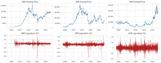
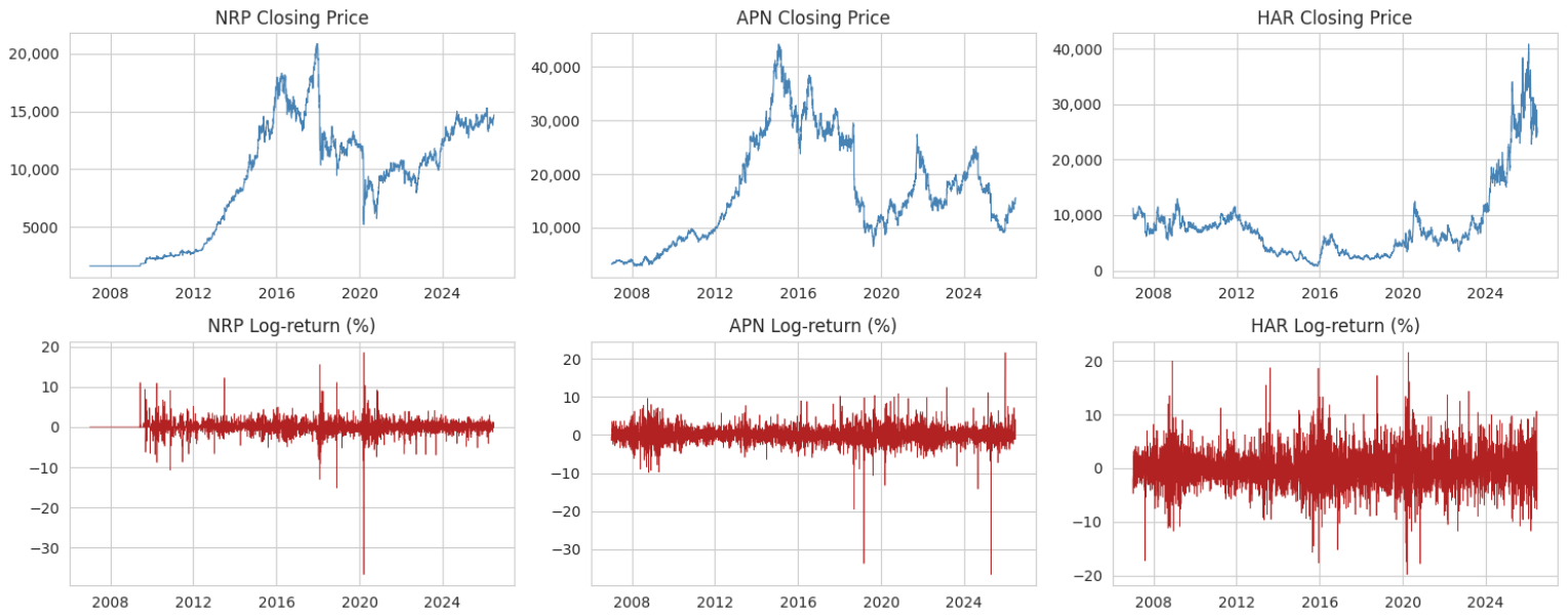
Figure 1 visualizes the price levels and log-return series for the three tickers given by NRP, APN and HAR from the JSE. The top row shows the closing price of each ticker over time. This shows the trend and price movements of each asset. The bottom row displays the log return (%) for each ticker. From these plots, there are periods of high and low volatility, which is often referred to as volatility clustering, where large changes tend to be followed by large changes and small changes by small changes. The clear presence of excess kurtosis is more frequent than a normal distribution would predict. This suggests “fat tails” in the log-return distribution, which imply the returns have a leptokurtotic distribution. More frequent large negative log-returns than large positive log-returns are evident for APN, which indicates that the distribution of log-returns is asymmetric.

Figure 1. Closing prices and log returns of NEPI Rockcastle N.V. (NRP), Aspen Pharmacare Holdings Limited (APN) and Harmony Gold Mining Company Limited (HAR).

3.1. Stylized Facts

Table 1 presents the formal descriptive and statistical test of the log-returns for the three stocks. Minimum (Min) and Maximum (Max) represent the largest daily losses and gains reported as log-returns. NRP and APN experienced extreme negative log-returns of approximately −36.7%, while HAR’s worst loss was −19.8%. APN recorded the highest positive return of 21.66%, suggesting substantial price fluctuations. All three stocks have positive average log-returns (Mean), although they are small (1.94–4.38%), indicating modest average daily profitability over the given period. NRP has the highest average return (4.38%). The standard deviation (Std.Dev.) measures volatility or the stock risk. HAR exhibits the highest volatility of 3.3714, followed by APN with 2.2072 and NRP with 1.6299. Thus, HAR is the riskiest stock among the three stocks. The negative skewness for NRP and APN implies that investors face a greater probability of experiencing unusually large negative returns compared to HAR. The exceptionally high kurtosis for NRP and APN indicates that these stocks exhibit substantial tail risk. HAR is the most volatile stock, while NRP displays the greatest downside asymmetry and the most pronounced tail risk. The Jarque–Bera (JB) test reveals that all stocks have p-values of 0.0000, leading to rejection of the null hypothesis of normality at conventional significance levels. This indicates that the return distributions are non-normal, consistent with the observed skewness and excess kurtosis. Since all ARCH-LM test p-values are below 0.05, the null hypothesis of constant variance is rejected. This suggests volatility clustering, where periods of high volatility tend to be followed by high volatility and periods of low volatility by low volatility. Consequently, GARCH-family models are appropriate for modeling these return series. All the Hurst exponent measures exceed 0.5, indicating strong persistence or long memory. This suggests that price movements tend to continue in the same direction rather than behaving as a purely random walk. Such persistence may imply some degree of predictability in return dynamics over the sample period. These findings imply that conventional models assuming normality and constant variance would be inadequate for these data. Instead, econometric models that accommodate fat tails, volatility clustering, and persistence, such as GARCH-family models with non-normal error distributions, would provide a more appropriate framework for modeling the return behavior of these stocks.

Table 1. Descriptive statistics and stylized facts diagnostics for log returns.

Stock	Min	Max	Mean	Std. Dev.	Skewness	Kurtosis	JB (p-Value)	ARCH-LM (p-Value)	Hurst ($\left|\mathit{r}\right|$)
NRP	−36.6779	18.5220	0.0438	1.6299	−2.3341	74.1090	0.0000	0.0000	0.8271
APN	−36.6873	21.6561	0.0291	2.2072	−1.5657	32.4224	0.0000	0.0054	0.8006
HAR	−19.8451	21.5412	0.0194	3.3714	0.1354	3.2095	0.0000	0.0000	0.8172

The annualized volatility estimates show considerable differences in risk across the three stocks. NRP recorded the lowest annualized volatility of 25.88%, indicating relatively stable returns and lower investment risk. APN exhibited moderate volatility of 35.04%, suggesting greater variability in returns. HAR recorded the highest annualized volatility of 53.53%, implying that its returns fluctuate substantially more than those of the other two stocks. Consequently, HAR represents the riskiest investment based on historical return variability, while NRP appears to be the least risky.

3.2. Model Estimation and Selection

To determine the most appropriate volatility model for each stock return series, several GARCH-family specifications, namely, GARCH, EGARCH, FIGARCH, HYGARCH, APARCH, FIAPARCH, and FIEGARCH, were estimated and compared using the Akaike Information Criterion (AIC) and Bayesian Information Criterion (BIC). These information criteria assess model performance by balancing goodness-of-fit with model complexity, with lower values indicating a more parsimonious and better model fit.

The findings in Table 2 are the results of the FIGARCH model that produced the lowest AIC and BIC values among the competing specifications for NRP, APN and HAR. This finding suggests that the volatility processes of all three stocks exhibit significant long-memory characteristics, where the effects of volatility shocks persist over extended periods, making the FIGARCH model the most appropriate specification for subsequent volatility modeling and analysis. The results provide consistent evidence in favor of the FIGARCH specification across all three securities. For NRP, FIGARCH produces the highest reported log-likelihood of 45,415.70 and the lowest AIC and BIC values of −90,823.40 and −90,797.39, respectively. Similarly, for APN, FIGARCH yields an AIC of −90,822.80 and a BIC of −90,796.78, while for HAR, the corresponding values are −90,821.95 and −90,795.93.

Table 2. Model selection specifications by stock series.

Stock	Model	Distribution	Log-Likelihood	AIC	BIC
NRP	GARCH	Empirical	45,414.15006	−90,822.3001	−90,802.7751
NRP	EGARCH	Empirical	603.267331	−1198.5347	−1172.5012
NRP	APARCH	Empirical	45,414.75006	−90,819.5001	−90,786.9584
NRP	FIGARCH	Empirical	45,415.6999	−90,823.3997	−90,797.3857
NRP	FIEGARCH	Empirical	24,790.11037	−49,572.2207	−49,546.1873
NRP	FIAPARCH	Empirical	45,414.75006	−90,817.5001	−90,778.4500
NRP	HYGARCH	Empirical	45,414.75006	−90,819.5001	−90,786.9584
APN	GARCH	Empirical	45,414.44551	−90,822.8910	−90,803.3660
APN	EGARCH	Empirical	0.443469273	7.1131	33.1465
APN	APARCH	Empirical	45,414.44551	−90,818.8910	−90,786.3493
APN	FIGARCH	Empirical	45,415.3966	−90,822.7933	−90,796.7793
APN	FIEGARCH	Empirical	2387.042179	−4766.0844	−4740.0509
APN	FIAPARCH	Empirical	45,414.44551	−90,816.8910	−90,777.8409
APN	HYGARCH	Empirical	45,414.44551	−90,818.8910	−90,786.3493
HAR	GARCH	Empirical	45,414.01992	−90,822.0398	−90,802.5148
HAR	EGARCH	Empirical	160.5211662	−313.0423	−287.0089
HAR	APARCH	Empirical	45,414.01992	−90,818.0398	−90,785.4981
HAR	FIGARCH	Empirical	45,414.9730	−90,821.9461	−90,795.9321
HAR	FIEGARCH	Empirical	1252.434838	−2496.8697	−2470.8363
HAR	FIAPARCH	Empirical	45,414.01992	−90,816.0398	−90,776.9897
HAR	HYGARCH	Empirical	45,414.01992	−90,818.0398	−90,785.4981

3.3. Risk Measure Estimates and VaR Backtesting with Adaptive Risk Limits

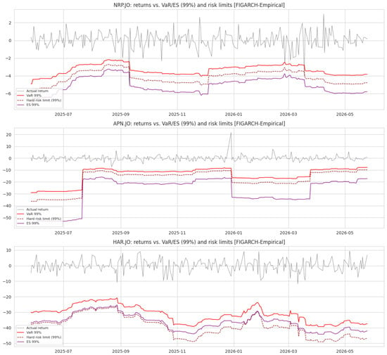
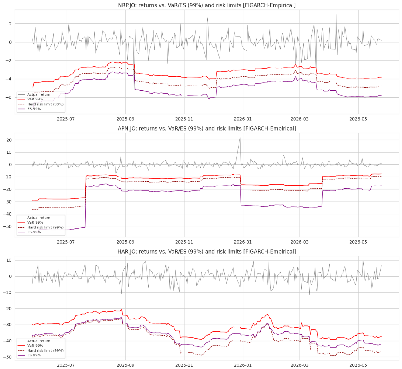
Figure 2 illustrates the out-of-sample path of the continuously compounded daily returns alongside the estimated 99% Value-at-Risk ($Va{R}_{0.99}$), Expected Shortfall ($E{S}_{0.99}$) and the proposed adaptive Hard Risk Limit ($RiskLimi{t}_{0.99}$) over the 250-day out-of-sample evaluation period. Across all three tickers, the $E{S}_{0.99}$ consistently tracks below the $Va{R}_{0.99}$ in the negative return space. This is mathematically consistent with the coherence property of Expected Shortfall, which evaluates the tail expectation conditional on a breach of the VaR threshold. A key feature of the APN panel is the pronounced step-like adjustments in the risk boundaries. Because the model is estimated using filtered historical simulation with an empirical innovation distribution, the historical outlier of $-36.69\%$ recorded during the in-sample period remains a dominant data point in the empirical quantile of the standardized residuals. Consequently, at the beginning of the forecasting window, the risk measures are extremely wide, with VaR near $-30\%$ and ES near $-53\%$. As the conditional volatility (${\sigma }_t$) decays, governed by the long-memory hyperbolic decay parameter d of the FIGARCH process, the risk limits step upward in discrete phases, reflecting a gradual structural decompression of risk. The behavior of the adaptive $RiskLimi{t}_{0.99}$ varies significantly across the three series, driven directly by the model’s out-of-sample forecasting performance.

Figure 2. 99% VaR, ES and risk limit for 250-day out-of-sample series.

For NRP, the realized out-of-sample violation rate was ${\widehat{\pi }}_F=0.012$, slightly exceeding the nominal target of $\alpha =0.01$7. In accordance with the adaptive framework defined in Equation (8), this underestimation triggers a penalty multiplier of $k=1.10$711. Visually, this is shown by the dashed brown line separating from the red VaR boundary and establishing a wider, more conservative capital buffer. For APN and HAR, the realized violation rates were ${\widehat{\pi }}_F=0.000$7. Because the models achieved perfect coverage, i.e., zero breaches, the adaptive multiplier remained at its minimum baseline of $k=1.00$, causing the risk limit to superimpose exactly onto the $Va{R}_{0.99}$ line. While safe, this visual gap highlights the extreme capital inefficiency of the filtered historical simulation approach in highly persistent volatility states.

Table 3 reports that the Kupiec p-value (K-p) for NRP at 95% and 99% is higher than the 5% significance level. This implies that violations are acceptable. However, the number of violations is inconsistent with the expected level of APN at 95%, as shown by a p-value < 5%. The Christoffersen conditional coverage test for NRP at 95% and 99% is insignificant (p-value = 0.70 and 0.79), suggesting that VaR exceptions occur independently over time. Therefore, the VaR model provides adequate risk forecasts. For APN at 95%, the exceptions are clustered, which suggests that the VaR model does not adequately capture the underlying risk dynamics. Furthermore, the statistical improvement of long-memory specifications is empirically supported by the backtesting comparison in Table 3. Across all three tickers, the calibration error of the FIGARCH empirical model ($c\text{\_}er{r}_F$) is lower than that of the standard benchmark GARCH model ($c\text{\_}er{r}_G$). For instance, at the 95% confidence level for NRP, FIGARCH yields a calibration error of 0.002 compared to 0.014 for GARCH, demonstrating the precision gained by incorporating fractional integration and empirical innovation distributions.

Table 3. Kupiec (K) proportion of failures (POF) and Christoffersen (C) independence-conditional coverage backtest results of VaR for FIGARCH model with empirical distribution on 250-day out-of-sample series.

Stock	Conf.	$\widehat{\mathit{\pi }}$	$\mathit{\alpha }$	K	K-p	C	C-p	${\widehat{\mathit{\pi }}}_{\mathit{G}}$	${\widehat{\mathit{\pi }}}_{\mathit{F}}$	$\mathit{c}\text{\_}{\mathit{err}}_{\mathit{G}}$	$\mathit{c}\text{\_}{\mathit{err}}_{\mathit{F}}$	State	HRLB
NRP	95%	0.052	0.05	0.0208	0.8853	0.1499	0.6986	0.036	0.052	0.014	0.002	$+c$	0.032
NRP	99%	0.012	0.01	0.0949	0.7580	0.0732	0.7868	0.008	0.012	0.002	0.002	$+c$	0.008
APN	95%	0.004	0.05	18.4966	0.0000	0.0081	0.9284	0.008	0.004	0.042	0.046	$-c$	0.004
APN	99%	0.000	0.01	NaN	NaN	−0.0000	1.0000	0.004	0.000	0.006	0.010	$-c$	0.000
HAR	95%	0.000	0.05	NaN	NaN	−0.0000	1.0000	0.080	0.000	0.030	0.050	$-c$	0.000
HAR	99%	0.000	0.01	NaN	NaN	−0.0000	1.0000	0.032	0.000	0.022	0.010	$+c$	0.000

$+c$ implies best model calibration and $-c$ implies possible distributional misspecification. Smaller deviation = better calibration. Improvement is observed to be more pronounced at 99%.

4. Discussion

The empirical findings of this study offer important insights for the implementation of market risk models under the Basel III/FRTB framework [2]. The comparative analysis presented in Table 2 reveals a crucial methodological challenge when fitting GARCH-type models with a non-parametric empirical likelihood. The APARCH, FIAPARCH and HYGARCH specifications yielded identical log-likelihood values to the fifth decimal place for NRP stock. Similarly, the GARCH, APARCH, FIAPARCH and HYGARCH specifications yielded identical log-likelihood values to the fifth decimal place for APN and HAR stocks. This optimization collapse occurs because non-parametric empirical likelihood functions are step-like and lack the smooth, analytical derivatives required for gradient-based optimization routines. Consequently, the algorithms failed to converge, collapsing to a homoskedastic baseline where all conditional volatility coefficients ($\alpha ,\beta$, or the fractional integration parameter d) were numerically constrained to zero. In contrast, the EGARCH and FIEGARCH models successfully converged because they model the natural logarithm of the conditional variance ($\ln {\sigma }_t^2$), which naturally avoids non-negativity constraints. This highlights that fitting GARCH-type models under empirical assumptions requires a two-stage Quasi-Maximum Likelihood Estimation approach, estimating the parameters with a parametric distribution such as standardized skewed Student-t and applying filtered historical simulation to the resulting standardized residuals.

The out-of-sample backtesting results reported in Table 3 provide a clear validation of the selected specifications. For NRP, the FIGARCH model with an empirical distribution demonstrates superior calibration. At the 95% confidence level, the realized violation rate (${\widehat{\pi }}_F=0.052$) is close to the nominal target ($\alpha =0.05$), yielding a minimal calibration error ($c\text{\_}er{r}_F=0.002$) compared to the standard GARCH model ($c\text{\_}er{r}_G=0.014$). This is denoted as a “+c” state, confirming optimal model calibration.

Conversely, for APN and HAR, the backtesting results at both the 95% and 99% levels generated “NaN” values for the Kupiec POF and Christoffersen conditional coverage tests. Econometrically, this “NaN” state occurs because the realized out-of-sample violation rate was exactly zero (${\widehat{\pi }}_F=0.000$). Since the likelihood ratio test statistics for both tests involve the natural logarithm of the violation rate ($\ln \left(\widehat{\pi }\right)$), the math becomes undefined at zero, indicating that no breaches occurred. While a zero-breach model is highly desirable from a safety perspective, it indicates a “−c” state known as a distributional misspecification. Thus, the risk limits are excessively wide and conservative. The rate of hard risk limit breaches (HRLB), particularly those that push a trading desk into the regulatory amber or red backtesting zones, is an important indicator of model risk. Such breaches can trigger higher capital requirements, increased supervisory scrutiny and, in more severe cases, the replacement of the internal model with the standardised approach. Under regulatory standards, maintaining such over-conservative risk boundaries forces a trading desk to hold an unnecessarily large, capital-inefficient regulatory buffer, violating the operational goals of active portfolio management.

The adaptive multiplier k introduced in Equation (8) successfully translates these statistical dynamics into operational boundaries. By scaling the risk limits dynamically when the violation rate exceeds the nominal target, as observed in the NRP 99% model where $k=1.10$, the framework replicates the supervisory penalty structure of the Basel Committee’s traffic-light system. This ensures that models that fail to capture tail risk are automatically restricted through wider boundaries, while parsimonious, well-calibrated models are rewarded with tighter, capital-efficient risk bands.

5. Conclusions

This paper has evaluated the empirical performance of long-memory and asymmetric GARCH-type models in estimating Value-at-Risk (VaR) and Expected Shortfall (ES) for three actively traded JSE equities with distinct risk profiles. By examining the performance of these specifications against standard GARCH(1,1) benchmarks, the study demonstrates that incorporating fractionally integrated structures, such as FIGARCH, significantly improves out-of-sample risk calibration when the return series exhibit strong volatility persistence and high Hurst exponents.

The theoretical contribution of this work lies in the formulation of an adaptive risk limit framework that mirrors the regulatory penalty structure of the Basel III/FRTB framework [2]. By defining the risk boundary as a function of the out-of-sample violation rate through a mathematical operator, we provide a mechanism that penalizes risk underestimation without relying on arbitrary, static multipliers. Practically, the results show that while the FIGARCH model with an empirical distribution provides exceptional calibration for stable series like NRP, it can generate overly conservative, capital-inefficient boundaries for assets characterized by historical extreme outliers, such as APN, due to the nature of filtered historical simulation [19].

Future research will expand this framework to a multivariate, portfolio-level context to account for dynamic asset correlations. Thus, incorporating the full Acerbi and Szekely multi-test battery for Expected Shortfall validation and performing systematic sensitivity analyses on rolling-window lengths to optimize the balance between capital efficiency and coverage safety [20].

References

- Kim, D.; Shin, M. Volatility models for stylized facts of high-frequency financial data. J. Time Ser. Anal. 2023, 44, 262–279. [Google Scholar] [CrossRef] [Scilit]
- Basel Committee on Banking Supervision. Minimum Capital Requirements for Market Risk; Technical Report; Bank for International Settlements: Basel, Switzerland, 2019. [Google Scholar]
- Cont, R. Empirical Properties of Asset Returns: Stylized Facts and Statistical Issues. Quant. Financ. 2001, 1, 223–236. [Google Scholar] [CrossRef]
- Thompson, S. The stylised facts of stock price movements. N. Z. Rev. Econ. Financ. 2011, 1, 50–77. [Google Scholar]
- Sen, R.; Subramaniam, M. Stylized facts of the Indian stock market. Asia-Pacific Financ. Mark. 2019, 26, 479–493. [Google Scholar] [CrossRef] [Scilit]
- Khumalo, M.; Mashele, H.; Seitshiro, M. Quantification of the stock market value at risk by using FIAPARCH, HYGARCH and FIGARCH models. Data Sci. Financ. Econ. 2023, 3, 380. [Google Scholar] [CrossRef] [Scilit]
- S’afari, S.A.; Janisch, M.; Lehéricy, T. International financial markets through 150 years: Evaluating stylized facts. J. Financ. Data Sci. 2026, 12, 100196. [Google Scholar] [CrossRef] [Scilit]
- Bollerslev, T. Generalized Autoregressive Conditional Heteroskedasticity. J. Econom. 1986, 31, 307–327. [Google Scholar] [CrossRef] [Scilit]
- Baillie, R.T.; Bollerslev, T.; Mikkelsen, H.O. Fractionally Integrated Generalized Autoregressive Conditional Heteroskedasticity. J. Econom. 1996, 74, 3–30. [Google Scholar] [CrossRef] [Scilit]
- Engle, R.F. Autoregressive Conditional Heteroscedasticity with Estimates of the Variance of United Kingdom Inflation. Econometrica 1982, 50, 987–1007. [Google Scholar] [CrossRef] [Scilit]
- Nelson, D.B. Conditional Heteroskedasticity in Asset Returns: A New Approach. Econometrica 1991, 59, 347–370. [Google Scholar] [CrossRef] [Scilit]
- Davidson, J. Moment and Memory Properties of Linear Conditional Heteroscedasticity Models, and a New Model. J. Bus. Econ. Stat. 2004, 22, 16–29. [Google Scholar] [CrossRef] [Scilit]
- Ding, Z.; Granger, C.W.J.; Engle, R.F. A Long Memory Property of Stock Market Returns and a New Model. J. Empir. Financ. 1993, 1, 83–106. [Google Scholar] [CrossRef] [Scilit]
- Tse, Y.K. The Conditional Heteroscedasticity of the Yen–Dollar Exchange Rate. J. Appl. Econom. 1998, 13, 49–55. [Google Scholar] [CrossRef]
- Zaevski, T.S.; Nedeltchev, D.C. From Basel III to Basel IV and Beyond: Expected Shortfall and Expectile Risk Measures. Int. Rev. Financ. Anal. 2023, 87, 102645. [Google Scholar] [CrossRef] [Scilit]
- Du, Z.; Pei, P.; Wang, X.; Yang, T. Powerful Backtests for Historical Simulation Expected Shortfall Models. J. Bus. Econ. Stat. 2024, 42, 864–874. [Google Scholar] [CrossRef] [Scilit]
- Kupiec, P.H. Techniques for Verifying the Accuracy of Risk Measurement Models. J. Deriv. 1995, 3, 73–84. [Google Scholar] [CrossRef] [Scilit]
- Christoffersen, P.F. Evaluating Interval Forecasts. Int. Econ. Rev. 1998, 39, 841–862. [Google Scholar] [CrossRef] [Scilit]
- Bayer, S.; Dimitriadis, T. Backtesting Value-at-Risk and Expected Shortfall in the Presence of Estimation Error. J. Financ. Econom. 2023, 21, 528–568. [Google Scholar] [CrossRef] [Scilit]
- Acerbi, C.; Szekely, B. Backtestability and the ridge backtest. In Peter Carr Gedenkschrift: Research Advances in Mathematical Finance; World Scientific: Singapore, 2024; pp. 61–100. [Google Scholar]
Disclaimer/Publisher’s Note: The statements, opinions and data contained in all publications are solely those of the individual author(s) and contributor(s) and not of MDPI and/or the editor(s). MDPI and/or the editor(s) disclaim responsibility for any injury to people or property resulting from any ideas, methods, instructions or products referred to in the content. |
© 2026 by the author. Licensee MDPI, Basel, Switzerland. This article is an open access article distributed under the terms and conditions of the Creative Commons Attribution (CC BY) license.