An Analysis and Global Identification of Smoothless Variable Order of a Fractional Stochastic Differential Equation

Abstract

We establish both the uniqueness and the existence of the solutions to a hidden-memory variable-order fractional stochastic partial differential equation, which models, e.g., the stochastic motion of a Brownian particle within a viscous liquid medium varied with fractal dimensions. We also investigate the inverse problem concerning the observations of the solutions, which eliminates the analytic assumptions on the variable orders in the literature of this topic and theoretically guarantees the reliability of the determination and experimental inference.

1. Introduction

Stochastic differential equations (SDEs) [1,2,3,4,5,6]

$$du=f\left(u\right)dt+\sigma \left(u\right)dB$$

(1)

prove to be a very powerful tool for modeling random phenomena that occur in the sciences, social sciences, engineering, and applications. For instance, they may be used to describe the erratic movement of a Brownian particle (of typically a sub-micron size) immersed in a surrounding viscous fluid because of the random and incessant bombardments of the much smaller and faster fluid molecules due to density fluctuation in the fluid. In this context, u refers to the jiggling velocity, $f\left(u\right)dt$ refers to the mean friction force due to the interaction of the Brownian particle with the surrounding medium during a very short time period $dt$ that is orders of magnitude smaller than the relaxation time-scale of the Brownian particle and $\sigma \left(u\right)dB$ denotes the effect of the background noise of the fluid during the time period due to its impact on the particle, per unit mass of the Brownian particle. Hence, the background noise has a mean of zero. Physically, individual collisions occur very rapidly (say, on the order of ${10}^6$ during the time period $dt$) and therefore are independent of each other and completely uncorrelated with no-time memory effects. Consequently, (1) provides a microscale description of a Brownian motion or equivalently a normal diffusive transport process.

However, the motion of a Brownian particle is a result of thermal fluctuations in the medium, which causes the particle to experience a series of random changes in direction and velocity, e.g., in the catoplasm of living cells often experience memory effects and exhibit anomalously diffusive or power-law transport behavior [7,8,9]. Fractional derivatives were introduced in fractional partial differential equations [10,11,12] or even fractional SDEs [13] to model the anomalously diffusive or power-law memory effect in the anomalously diffusive transport processes, which attracts growing research activities on fractional SDEs [14,15,16,17].

Fractional SDEs (FSDEs) are widely used in modeling complicated scenarios in, e.g., physics, control theory, and mechanics. The FSDEs can be considered as a natural extension of the conventional SDEs [10,15]. Recently, Huang et al. [18] investigated the well-posedness of solutions for the multiterm FSDEs and developed the corresponding fast algorithm. Zhao et al. [19] extended the spectral method for FSDEs by using the dynamically orthogonal/orthogonal decompostion. Additionally, the fast Euler–Maruyama method for Riemann–Liouville FSDEs was proposed and analyzed in [20,21]. Furthermore, the Brownian particle and the molecules of the surrounding medium could cause structural changes and so the fractal dimension of the medium [22,23], and hence the fractional order, would change via the Hurst index [23,24,25], leading to variable-order fractional problems [26,27,28,29].

Consequently, we consider the hidden-memory variable-order nonlinear FSDE

$$du=\left(\lambda {\partial }_t^{\kappa \left(t\right)}u+f\left(u\right)\right)dt+\sigma \left(u\right)dB,t\in (0,T];u\left(0\right)=u_0.$$

(2)

Here, $\lambda \in \mathbb{R}$, f and $\sigma$ refer to deterministic functions, $B\left(t\right)$ represents the Brownian motion, and we define the hidden-memory variable-order fractional derivative ${\partial }_t^{\kappa \left(t\right)}$ of order $0\le \kappa <1$ as follows [24,26]:

$$\begin{array}{cc}\hfill {\partial }_t^{\kappa \left(t\right)}u& {\displaystyle :={\partial }_t{\partial }_t^{-(1-\kappa (t\left)\right)}u,}\hfill \\ \hfill {\partial }_t^{-(1-\kappa (t\left)\right)}u& {\displaystyle :={\int }_0^t\frac{u\left(\zeta \right)d\zeta }{\mathrm{\Gamma }(1-\kappa \left(\zeta \right)){(t-\zeta )}^{\kappa \left(\zeta \right)}}.}\hfill \end{array}$$

(3)

Here,

$$\mathrm{\Gamma }\left(\zeta \right):={\int }_0^{\infty }{\theta }^{\zeta -1}{e}^{-\theta }d\theta .$$

For each $t\in [0,T]$, the variable order $\kappa$ inside the integral from 0 to time t assumes its value $\kappa \left(\zeta \right)$ as s evolves on $[0,t]$. That is, ${\partial }_t^{\kappa \left(\zeta \right)}$ at time $\zeta \in [0,T]$ is defined as the integrated impact of the order history quantified by the order $\kappa \left(\zeta \right)$ over $[0,t]$.

In most circumstances, the fractional order $\kappa$ has to be inferred from the measurements instead of being provided a prior. The inverse problems which aim at identifying the parameters in fractional PDEs present some new issues that have attracted an increasing number of research activities, although rigorous mathematical analysis and numerical identifications on the identification of fractional orders in fractional PDEs have been conducted for constant-order fractional PDEs [30,31,32,33,34,35,36,37,38,39,40] as well as variable-order fractional partial differential equations [41,42,43,44].

Another merit of the current work consists in reducing the smoothness assumptions on the variable fractional order when proving its unique identification. In some very recent works [44], the $\kappa \left(t\right)$ in FPDEs are uniquely determined under the assumption that the variable orders are analytic functions. In many circumstances, this condition is quite restrictive as the variable orders may be smoothless or even discontinuous in real applications, such as anomalous diffusion in heterogeneous media, and the fractal structure (and thus the fractional order in governing equations [23]) of which may differ at different locations. In this work, we develop different techniques to establish the uniqueness of the global identification of variable order in fractional SDEs without any smoothness assumption on the variable fractional order.

2. Preliminaries

This section introduces the preliminaries to be used subsequently. Let $0\le c<d<\infty$ and $L^2(c,d)$ and $L^{\infty }(c,d)$ be spaces of functions that are square-integrable and bounded almost everywhere, respectively, equipped with the norms [45]

$${\displaystyle {\parallel R\parallel }_{L^2(c,d)}:={\left({\int }_c^{d}R{\left(t\right)}^{2}dt\right)}^{1/2}{,\parallel R\parallel }_{L^{\infty }(c,d)}:=\mathrm{ess}\underset{t\in [c,d]}{sup}\left|R\left(t\right)\right|.}$$

In problem (2) B is a Brownian motion defined on a complete probability space $(\mathrm{\Omega },ℱ,P)$, $u_0$ is a second-order random variable, i.e.,

$$\mathbb{E}\left[u_0^2\right]:={\int }_{\Omega }{u}_0{\left(\omega \right)}^{2}dP\left(\omega \right)<\infty ,$$

which assumes to be independent of $B\left(t\right)$, and $ℱ\left(t\right):=\mathcal{U}\{B\left(s\right)(0\le s\le t),u_0\}$ is the $\sigma$-algebra generated by $u_0$ [1,4].

Throughout the paper, we presume that:

(A)

$0\le \kappa \left(t\right)\le {\kappa }^{*}$ on $[0,T]$ for some $0\le {\kappa }^{*}<1$,

(B)

f and g satisfy the Lipschitz continuity and the following growth condition for some constant $L>0$:

$$\begin{array}{cc}\left|f\right(v\left)\right|+\left|\sigma \right(v\left)\right|\le L(1+|v\left|\right),& \forall v\in \mathbb{R},\\ |f\left(v_1\right)-f\left(v_2\right)|+|\sigma \left(v_1\right)-\sigma \left(v_2\right)|\le L|v_1-v_2|,& \forall v_1,v_2\in \mathbb{R}.\end{array}$$

In addition to (3), in this paper we also need [24,26]

$$*{\partial }_t^{-(1-\kappa (t\left)\right)}u:={\int }_0^t\frac{u\left(\zeta \right)d\zeta }{\mathrm{\Gamma }(1-\kappa \left(t\right)){(t-\zeta )}^{\kappa \left(t\right)}}.$$

(4)

The $*{\partial }_t^{-(1-\kappa (t\left)\right)}u$ in (4) accounts for the integrated impact of the nonlocal fading memory of order $\kappa \left(t\right)$ on the solution u, where the variable order $\kappa$ presumes its value $\kappa \left(t\right)$ at the upper limit t of the integral instead of the value $\kappa \left(s\right)$ at time instant $s\in [0,t]$. In contrast, of the hidden-memory variable-order fractional integral operator ${\partial }_t^{-(1-\kappa (t\left)\right)}u$ accounts for the integrated impact of the non-local fading memory weighted at the time instant s, which gives a physically more relevant description of memory effect and, thus, motivates the study the hidden-memory variable-order fractional SDE (3). Note that the kernel in (3) exhibits salient features of the hidden memory effect and significantly complicates the corresponding mathematical analysis.

Lemma 1

(Gronwall inequality with weak singular kernel [46]). Suppose $C_0\left(t\right)\ge 0$ is a non-decreasing function, which is locally integrable on $(a,b]$ and $C_1\ge 0$. Suppose $g\ge 0$ is a locally integrable function on $(a,b]$ such that

$$g\left(t\right)\le C_0\left(t\right)+C_1{\int }_a^t\frac{g\left(\zeta \right)d\zeta }{{(t-\zeta )}^{1-\gamma }},\forall t\in (a,b],0<\gamma <1,$$

then

$$g\left(t\right)\le C_0\left(t\right)E_{\gamma }\left(C_1\mathrm{\Gamma }\left(\gamma \right){(t-a)}^{\gamma }\right),\forall t\in (a,b],$$

where [10,12,47]

$$E_{\gamma }\left(z\right):={\displaystyle \sum _{k=0}^{\infty }}\frac{z^k}{\mathrm{\Gamma }(\gamma k+1)},z\in \mathbb{R},\gamma \in {\mathbb{R}}^{+}.$$

(5)

Lemma 2

(The Burkhölder–Davis–Gundy inequality [6,48]). We assume that X is a continuous martingale, and then there must exist a constant $Q\left(p\right)>0$ for $1\le p<\infty$ such that

$$\mathbb{E}\left[\underset{s\in [0,t]}{max}{\left|X\left(s\right)\right|}^p\right]\le Q\left(p\right)\mathbb{E}\left[{\left|X\left(t\right)\right|}^p\right],0\le t\le T.$$

3. Analysis of the SDE (2)

The well-posedness of the hidden-memory variable-order fractional SDE (2) and the regularity estimate of its solution have been proved. The variable-order fractional SDEs with the variable-order integral operator $*{\partial }_t^{-(1-\kappa (t\left)\right)}$ given in (4) have appeared in some of the literature (see, e.g., [14,15,16,17,49]). However, there is no report in the literature on rigorous mathematical analysis of the variable-order fractional SDEs.

Our analysis starts with the following lemma.

Lemma 3.

For $0<r<1$, let $Q=Q\left(r\right)$ be a positive constant such that for any $n\ge 1$

$$S_n:=\sum _{j=0}^{n-1}\frac{1}{\mathrm{\Gamma }\left((n-j-1)r+1\right)\mathrm{\Gamma }(jr+1)}\le \frac{Q}{\mathrm{\Gamma }\left(\right(n-1)r/2+1)}.$$

Proof. 

It is known that $\mathrm{\Gamma }\left(x\right)$ attains its minimum at $x_0\approx 1.46$ on $(0,\infty )$. Define

$${\displaystyle n_0:=1+⌊1+\frac{2(x_0-1)}{r}⌋,}$$

where $\lfloor x\rfloor$ represents the floor of x, such that $(n_0-1)r/2+1>x_0$. We first consider the case $n>n_0$ and split $S_n$ into the two parts

$$\begin{array}{cc}{S}_n\hfill & {\displaystyle :=\sum _{j<(n-1)/2}\frac{1}{\mathrm{\Gamma }\left((n-j-1)r+1\right)\mathrm{\Gamma }(jr+1)}}\hfill \\ \hfill & {\displaystyle +\sum _{j\ge (n-1)/2}\frac{1}{\mathrm{\Gamma }\left((n-j-1)r+1\right)\mathrm{\Gamma }(jr+1)}.}\hfill \end{array}$$

For $j<(n-1)/2$, $(n-j-1)r+1>(n-1)r/2+1>x_0$. Use the monotonicity of the Gamma function to obtain

$$\begin{array}{c}{\displaystyle \sum _{j<(n-1)/2}\frac{1}{\mathrm{\Gamma }\left((n-j-1)r+1\right)\mathrm{\Gamma }(jr+1)}}\hfill \\ {\displaystyle \le \frac{1}{\mathrm{\Gamma }\left(\right(n-1)r/2+1)}\sum _{j<(n-1)/2}\frac{1}{\mathrm{\Gamma }(jr+1)}}\hfill \\ {\displaystyle \le \frac{E_r\left(1\right)}{\mathrm{\Gamma }\left(\right(n-1)r/2+1)}.}\hfill \end{array}$$

Similarly, $j\ge (n-1)/2$ implies $jr+1\ge (n-1)r/2+1>x_0$. Consequently,

$$\begin{array}{c}{\displaystyle \sum _{j\ge (n-1)/2}\frac{1}{\mathrm{\Gamma }\left((n-j-1)r+1\right)\mathrm{\Gamma }(jr+1)}}\hfill \\ {\displaystyle \le \frac{1}{\mathrm{\Gamma }\left(\right(n-1)r/2+1)}\sum _{j\ge (n-1)/2}\frac{1}{\mathrm{\Gamma }\left(\right(n-j-1)r+1)}}\hfill \\ {\displaystyle \le \frac{E_{r,1}\left(1\right)}{\mathrm{\Gamma }\left(\right(n-1)r/2+1)}.}\hfill \end{array}$$

Combining the two estimates yields the proof for $n>n_0$. As for the case $n\le n_0$, note that there exist only a finite number of terms satisfying $n\le n_0$. We can enforce the inequality by properly selecting the constant Q. □

As in the classical SDEs [1,4], problem (2) is formulated as follows: Identify a stochastic process u which is progressively measurable concerning $ℱ(·)$ such that

$$u\left(t\right)-u_0=\left(\mathcal{L}u\right)\left(t\right):=\lambda {\partial }_t^{-(1-\kappa (t\left)\right)}u+{\int }_0^{t}f\left(u\left(\zeta \right)\right)d\zeta +{\int }_0^t\sigma \left(u\left(\zeta \right)\right)dB\left(\zeta \right),$$

(6)

where we have used the fact that integrating both sides of (2) from 0 to t and applied the definition of the fractional operator definied by (3).

Theorem 1.

Let assumptions (A)–(B) hold and $u_0$ represent a second-order random variable. Then, there exists a unique solution u which satisfies the following stability estimate to problem (6):

$$\underset{t\in [0,T]}{sup}\mathbb{E}\left[u^2\right]\le Q\left(\mathbb{E}\left[u_0^2\right]+1\right).$$

(7)

Here, $Q=Q({\kappa }^{*},\lambda ,L,T)$.

Proof. 

Motivated by formulation (6), Let us apply a successive approximation ${\left\{{\mathrm{\Phi }}_i\right\}}_{i=0}^{\infty }$ by

$${\mathrm{\Phi }}_i\left(t\right):={\mathrm{\Phi }}_0+\mathcal{L}{\mathrm{\Phi }}_{i-1}\left(t\right),n\ge 1$$

(8)

with ${\mathrm{\Phi }}_0\left(t\right):=u_0$. The theorem has been proved in four steps.

• Step 1: Convergence of ${\left\{{\mathrm{\Phi }}_i\right\}}_{i=0}^{\infty }$ in $L^2(\mu \times P)$

Here, $\mu$ is the Lebesgue measure on $[0,T]$. We subtract Equation (8) with i replaced by $i-1$ from Equation (8) for $i\ge 2$ to obtain

$$\begin{array}{cc}{\displaystyle {({\mathrm{\Phi }}_i\left(t\right)-{\mathrm{\Phi }}_{i-1}\left(t\right))}^2}\hfill & {\displaystyle ={\left(\mathcal{L}{\mathrm{\Phi }}_{i-1}\left(t\right)-\mathcal{L}{\mathrm{\Phi }}_{i-2}\left(t\right)\right)}^2}\hfill \\ \hfill & {\displaystyle \le 3{\lambda }^2{\left({\partial }_t^{-(1-\kappa (t\left)\right)}({\mathrm{\Phi }}_{i-1}-{\mathrm{\Phi }}_{i-2})\right)}^2}\hfill \\ \hfill & {\displaystyle +3{\left({\int }_0^t\left(f\left({\mathrm{\Phi }}_{i-1}\left(s\right)\right)-f\left({\mathrm{\Phi }}_{i-2}\left(s\right)\right)\right)ds\right)}^2}\hfill \\ \hfill & {\displaystyle +3{\left({\int }_0^t\left(\sigma \left({\mathrm{\Phi }}_{i-1}\left(s\right)\right)-\sigma \left({\mathrm{\Phi }}_{i-2}\left(s\right)\right)\right)dB\left(s\right)\right)}^2.}\hfill \end{array}$$

(9)

We apply assumptions (A) and (B) and the estimate

$$\begin{array}{c}{\displaystyle |{\partial }_t^{-(1-\kappa (t\left)\right)}({\mathrm{\Phi }}_{i-1}\left(t\right)-{\mathrm{\Phi }}_{i-2}\left(t\right)){|}^2}\hfill \\ {\displaystyle =|{\int }_0^t\frac{{(t-s)}^{{\kappa }^{*}-\kappa \left(s\right)}({\mathrm{\Phi }}_{i-1}\left(s\right)-{\mathrm{\Phi }}_{i-2}\left(s\right))ds}{\mathrm{\Gamma }(1-\kappa \left(s\right)){(t-s)}^{{\kappa }^{*}}}{|}^2}\hfill \\ \le Q{\left({\int }_0^t\frac{\left|{\mathrm{\Phi }}_{i-1}\right(s)-{\mathrm{\Phi }}_{i-2}(s\left)\right|ds}{{(t-s)}^{{\kappa }^{*}}}\right)}^2\hfill \\ \le Q{\int }_0^t\frac{ds}{(t-s{)}^{{\kappa }^{*}}}{\int }_0^t\frac{\left({\mathrm{\Phi }}_{i-1}\right(s)-{\mathrm{\Phi }}_{i-2}(s){)}^{2}ds}{(t-s{)}^{{\kappa }^{*}}}\hfill \\ \le Q{\int }_0^t\frac{\left({\mathrm{\Phi }}_{i-1}\right(s)-{\mathrm{\Phi }}_{i-2}(s){)}^{2}ds}{(t-s{)}^{{\kappa }^{*}}}\hfill \end{array}$$

(10)

to bound the right-hand side of (9) by

$$\begin{array}{cc}{\displaystyle {({\mathrm{\Phi }}_i\left(t\right)-{\mathrm{\Phi }}_{i-1}\left(t\right))}^2}\hfill & {\displaystyle \le Q{\int }_0^t\left(\frac{1}{{(t-s)}^{{\kappa }^{*}}}+t\right){({\mathrm{\Phi }}_{i-1}\left(s\right)-{\mathrm{\Phi }}_{i-2}\left(s\right))}^{2}ds}\hfill \\ \hfill & {\displaystyle +3{\left({\int }_0^t\left(\sigma \left({\mathrm{\Phi }}_{i-1}\left(s\right)\right)-\sigma \left({\mathrm{\Phi }}_{i-2}\left(s\right)\right)\right)dB\right)}^2.}\hfill \end{array}$$

(11)

We apply the Itô isometry and the Lipschitz continuity of $\sigma$ to bound the last term on the right-hand side by

$$\begin{array}{c}{\displaystyle \mathbb{E}\left[{\left({\int }_0^t\left(\sigma \left({\mathrm{\Phi }}_{i-1}\left(s\right)\right)-\sigma \left({\mathrm{\Phi }}_{i-2}\left(s\right)\right)\right)dB\right)}^2\right]}\hfill \\ {\displaystyle =\mathbb{E}\left[{\int }_0^t{\left(\sigma \left({\mathrm{\Phi }}_{i-1}\left(s\right)\right)-\sigma \left({\mathrm{\Phi }}_{i-2}\left(s\right)\right)\right)}^{2}ds\right]}\hfill \\ {\displaystyle \le Q{\int }_0^t\mathbb{E}\left[{\left({\mathrm{\Phi }}_{i-1}\left(s\right)-{\mathrm{\Phi }}_{i-2}\left(s\right)\right)}^2\right]ds.}\hfill \end{array}$$

(12)

We take expectations on both sides of (11) and use estimate (12) to estimate

$$\begin{array}{c}\mathbb{E}\left[{\left({\mathrm{\Phi }}_i\left(t\right)-{\mathrm{\Phi }}_{i-1}\left(t\right)\right)}^2\right]\hfill \\ {\displaystyle \le Q{\int }_0^t\left(\frac{1}{{(t-s)}^{{\kappa }^{*}}}+t\right)\mathbb{E}\left[{\left({\mathrm{\Phi }}_{i-1}\left(s\right)-{\mathrm{\Phi }}_{i-2}\left(s\right)\right)}^2\right]ds}\hfill \\ {\displaystyle \le \frac{Q_1}{\mathrm{\Gamma }(1-{\kappa }^{*})}{\int }_0^t\frac{\mathbb{E}\left[{\left({\mathrm{\Phi }}_{i-1}\left(s\right)-{\mathrm{\Phi }}_{i-2}\left(s\right)\right)}^2\right]ds}{{(t-s)}^{{\kappa }^{*}}},i\ge 2.}\hfill \end{array}$$

(13)

Here, $Q_1=Q_1({\kappa }^{*},\lambda ,L)$. We similarly bound

$$\mathbb{E}\left[{\left({\mathrm{\Phi }}_1\left(t\right)-{\mathrm{\Phi }}_0\left(t\right)\right)}^2\right]\le Q_2\left(1+\mathbb{E}\left[u_0^2\right]\right).$$

(14)

A mathematical induction from (13) and (14) concludes that

$$\mathbb{E}\left[{\left({\mathrm{\Phi }}_i\left(t\right)-{\mathrm{\Phi }}_{i-1}\left(t\right)\right)}^2\right]\le \frac{Q_2{\left(Q_1{t}^{1-{\kappa }^{*}}\right)}^{i-1}\left(1+\mathbb{E}\left[u_0^2\right]\right)}{\mathrm{\Gamma }((i-1)(1-{\kappa }^{*})+1)},t\in [0,T].$$

(15)

Then, for any $j>i\ge 1$

$$\begin{array}{c}{\displaystyle \parallel {\mathrm{\Phi }}_j-{\mathrm{\Phi }}_i{\parallel }_{L^2(\mu \times P)}= \parallel \sum _{k=i+1}^j({\mathrm{\Phi }}_k-{\mathrm{\Phi }}_{k-1}){\parallel }_{L^2(\mu \times P)}}\hfill \\ {\displaystyle \le \sum _{k=i+1}^j{\parallel {\mathrm{\Phi }}_k-{\mathrm{\Phi }}_{k-1}\parallel }_{L^2(\mu \times P)}}\hfill \\ {\displaystyle =\sum _{k=i+1}^m{\left(\mathbb{E}\left[{\int }_0^T{|{\mathrm{\Phi }}_k\left(t\right)-{\mathrm{\Phi }}_{k-1}\left(t\right)|}^{2}dt\right]\right)}^{1/2}}\hfill \\ {\displaystyle \le \sum _{k=i+1}^m{\left(\frac{Q_2{T}^{1-{\kappa }^{*}}{\left(Q_1{T}^{1-{\kappa }^{*}}\right)}^{k-1}\left(1+\mathbb{E}\left[u_0^2\right]\right)}{\mathrm{\Gamma }((k-1)(1-{\kappa }^{*})+2)}\right)}^{1/2}\to 0,}\hfill \end{array}$$

as $i,j\to \infty$. Namely, the successive approximation sequence ${\left\{{\mathrm{\Phi }}_i\right\}}_{i=0}^{\infty }$ is a Cauchy sequence in $L^2(\mu \times P)$. Thus, we assume $u\in L^2(\mu \times P)$ to be a limit function such that

$$\underset{i\to \infty }{lim}{\parallel {\mathrm{\Phi }}_i-u\parallel }_{L^2(\mu \times P)}=0.$$

(16)

We combine Assumptions (A) and (B), Ito isometry and (16) to deduce that as $i\to \infty$

$$\begin{array}{c}{\displaystyle \mathbb{E}\left[{\left({\int }_0^{t}f\left({\mathrm{\Phi }}_i\left(s\right)\right)ds-{\int }_0^{t}f\left(u\left(s\right)\right)ds\right)}^2\right]}\hfill \\ {\displaystyle \le L^{2}T\mathbb{E}\left[{\int }_0^T{|{\mathrm{\Phi }}_i\left(t\right)-u\left(t\right)|}^{2}dt\right]=L^{2}T{\parallel {\mathrm{\Phi }}_n-u\parallel }_{L^2(\mu \times P)}^2\to 0,}\hfill \\ {\displaystyle \mathbb{E}\left[{\left({\int }_0^t\sigma \left({\mathrm{\Phi }}_i\left(s\right)\right)dB\left(s\right)-{\int }_0^t\sigma \left(u\left(s\right)\right)dB\left(s\right)\right)}^2\right]}\hfill \\ {\displaystyle =\mathbb{E}\left[{\left({\int }_0^t\left(\sigma \left({\mathrm{\Phi }}_i\left(s\right)\right)-\sigma \left(u\left(s\right)\right)\right)dB\left(s\right)\right)}^2\right]}\hfill \\ {\displaystyle \le \mathbb{E}\left[{\int }_0^T{\left(\sigma \left({\mathrm{\Phi }}_i\left(s\right)\right)-\sigma \left(u\left(s\right)\right)\right)}^{2}ds\right]}\hfill \\ {\displaystyle \le L^2\mathbb{E}\left[{\int }_0^T{\left({\mathrm{\Phi }}_i\left(s\right)-u\left(s\right)\right)}^{2}ds\right]=L^2{\parallel {\mathrm{\Phi }}_n-u\parallel }_{L^2(\mu \times P)}^2\to 0.}\hfill \end{array}$$

(17)

• Step 2: Boundness of $\mathbb{E}\left[\underset{t\in [0,T]}{max}{\left({\mathrm{\Phi }}_i\left(t\right)-{\mathrm{\Phi }}_{i-1}\left(t\right)\right)}^2\right]$

To accomplish this, let

$$\begin{array}{cc}{G}_n\hfill & {\displaystyle :=3\underset{t\in [0,T]}{max}{\left({\int }_0^t\left(\sigma \left({\mathrm{\Phi }}_{i-1}\left(s\right)\right)-\sigma \left({\mathrm{\Phi }}_{i-2}\left(s\right)\right)\right)dB\left(s\right)\right)}^2}\hfill \\ G_1\hfill & {\displaystyle :=3\underset{t\in [0,T]}{max}{\left({\int }_0^t\sigma \left({\mathrm{\Phi }}_0\left(s\right)\right)dB\left(s\right)\right)}^2.}\hfill \end{array}$$

(18)

We use Lemma 2, Ito’s isometry, Assumption ((B)) and (8) to bound $G_1$ by

$$\begin{array}{cc}{\displaystyle \mathbb{E}\left[G_1\right]}\hfill & {\displaystyle \le Q\mathbb{E}\left[{\left({\int }_0^T\sigma \left(u_0\right)dB\left(s\right)\right)}^2\right]}\hfill \\ \hfill & {\displaystyle =Q\mathbb{E}\left[{\int }_0^T\sigma {\left(u_0\right)}^{2}dt\right]\le Q\left(1+\mathbb{E}\left[u_0^2\right]\right).}\hfill \end{array}$$

(19)

We combine (11) and (19) to obtain

$$\begin{array}{c}{\displaystyle \mathbb{E}\left[\underset{t\in [0,T]}{max}{\left({\mathrm{\Phi }}_1\left(t\right)-{\mathrm{\Phi }}_0\left(t\right)\right)}^2\right]}\hfill \\ {\displaystyle \le Q\left(1+\mathbb{E}\left[u_0^2\right]\right)+Q\mathbb{E}\left[\underset{t\in [0,T]}{max}{\left({\int }_0^t\sigma \left(u_0\right)dB\left(s\right)\right)}^2\right]}\hfill \\ {\displaystyle \le Q_2\left(1+\mathbb{E}\left[u_0^2\right]\right).}\hfill \end{array}$$

(20)

Here, we use the same positive constant $Q_2$ as in (14) and (15). In case the constant is larger than $Q_2$, we enlarge the constant $Q_2$ in (14) and (15).

We directly obtain from (11)

$${\left({\mathrm{\Phi }}_i\left(t\right)-{\mathrm{\Phi }}_{i-1}\left(t\right)\right)}^2\le Q_3{\int }_0^t\frac{{\left({\mathrm{\Phi }}_{i-1}\left(s\right)-{\mathrm{\Phi }}_{i-2}\left(s\right)\right)}^{2}ds}{{(t-s)}^{{\kappa }^{*}}}+G_n,n\ge 2.$$

(21)

Here, the constant $Q_3=Q_3({\kappa }^{*},\lambda ,L)$. Then, similar inductive arguments to estimate (15) yield the following sample path estimate for ${\left({\mathrm{\Phi }}_i\left(t\right)-{\mathrm{\Phi }}_{i-1}\left(t\right)\right)}^2$ based on (21)

$${\left({\mathrm{\Phi }}_i\left(t\right)-{\mathrm{\Phi }}_{i-1}\left(t\right)\right)}^2\le \sum _{j=1}^i\frac{{\left(Q_3{t}^{1-{\kappa }^{*}}\right)}^{i-j}{G}_j}{\mathrm{\Gamma }((n-j)(1-{\kappa }^{*})+1)},i\ge 1.$$

(22)

We use Lemma 2, (15), and the second estimate in (17), with u replaced by ${\mathrm{\Phi }}_{n-1}$, to bound $\mathbb{E}\left[G_n\right]$ for $n\ge 2$ by

$$\begin{array}{cc}{\displaystyle \mathbb{E}\left[G_i\right]}\hfill & {\displaystyle \le 3\mathbb{E}\left[\underset{t\in [0,T]}{max}{\left({\int }_0^t\left(\sigma \left({\mathrm{\Phi }}_{i-1}\left(s\right)\right)-\sigma \left({\mathrm{\Phi }}_{i-2}\left(s\right)\right)\right)dB\left(s\right)\right)}^2\right]}\hfill \\ \hfill & {\displaystyle \le Q\mathbb{E}\left[{\left({\int }_0^T\left(\sigma \left({\mathrm{\Phi }}_{i-1}\left(s\right)\right)-\sigma \left({\mathrm{\Phi }}_{i-2}\left(s\right)\right)\right)dB\left(s\right)\right)}^2\right]}\hfill \\ \hfill & {\displaystyle =Q\mathbb{E}\left[{\int }_0^T{\left(\sigma \left({\mathrm{\Phi }}_{i-1}\left(s\right)\right)-\sigma \left({\mathrm{\Phi }}_{i-2}\left(s\right)\right)\right)}^{2}ds\right]}\hfill \\ \hfill & {\displaystyle \le Q{\int }_0^T\mathbb{E}\left[{({\mathrm{\Phi }}_{i-1}\left(s\right)-{\mathrm{\Phi }}_{i-2}\left(s\right))}^2\right]ds}\hfill \\ \hfill & {\displaystyle \le \frac{Q{Q}_{2}T{\left(Q_1{T}^{1-{\kappa }^{*}}\right)}^{i-2}\left(1+\mathbb{E}\left[u_0^2\right]\right)}{\mathrm{\Gamma }((i-2)(1-{\kappa }^{*})+2)}.}\hfill \end{array}$$

(23)

We first take the maximum of estimate (22) in time and then its expectation, next combine the resulting inequality with estimates (19) and (23), and finally utilize Lemma 3 to achieve the following estimate:

$$\begin{array}{c}{\displaystyle \mathbb{E}\left[\underset{t\in [0,T]}{max}{\left({\mathrm{\Phi }}_i\left(t\right)-{\mathrm{\Phi }}_{i-1}\left(t\right)\right)}^2\right]\le \sum _{j=1}^i\frac{{\left(Q_3{T}^{1-{\kappa }^{*}}\right)}^{n-j}\mathbb{E}\left[G_j\right]}{\mathrm{\Gamma }((i-j)(1-{\kappa }^{*})+1)}}\hfill \\ {\displaystyle \le \frac{Q{\left(Q_3{T}^{1-{\kappa }^{*}}\right)}^{i-1}(1+\mathbb{E}\left[u_0^2\right])}{\mathrm{\Gamma }((i-1)(1-{\kappa }^{*})+1)}}\hfill \\ {\displaystyle +QT\sum _{j=2}^n\frac{{\left(Q_3{T}^{1-{\kappa }^{*}}\right)}^{i-j}}{\mathrm{\Gamma }((i-j)(1-{\kappa }^{*})+1)}\frac{Q_2{\left(Q_1{T}^{1-{\kappa }^{*}}\right)}^{j-2}(1+\mathbb{E}\left[u_0^2\right])}{\mathrm{\Gamma }((j-2)(1-{\kappa }^{*})+1)}}\hfill \\ {\displaystyle \le \frac{Q{\left(Q_3{T}^{1-{\kappa }^{*}}\right)}^{i-1}(1+\mathbb{E}\left[u_0^2\right])}{\mathrm{\Gamma }((i-1)(1-{\kappa }^{*})+1)}+\frac{Q{Q}_2{\left(Q_4{T}^{1-{\kappa }^{*}}\right)}^{i-2}(1+\mathbb{E}\left[u_0^2\right])}{\mathrm{\Gamma }((i-2)(1-{\kappa }^{*})/2+1)}}\hfill \\ {\displaystyle \le \frac{Q{\left(Q_4{T}^{1-{\kappa }^{*}}\right)}^{i-2}(1+\mathbb{E}\left[u_0^2\right])}{\mathrm{\Gamma }((i-2)(1-{\kappa }^{*})/2+1)},Q_4:=max\{Q_1,Q_3\},i\ge 2.}\hfill \end{array}$$

(24)

• Step 3: Existence of a solution to problem (3)

Now, we are able to prove the existence of a solution u to problem (3). By means of the Chebyshev’s inequality and estimates (24)

$$\begin{array}{cc}\hfill & {\displaystyle P\left(\underset{t\in [0,T]}{max}\left|{\mathrm{\Phi }}_i\left(t\right)-{\mathrm{\Phi }}_{i-1}\left(t\right)\right|\ge 2^{-n}\right)\le {\left(2^i\right)}^2\mathbb{E}\left[\underset{t\in [0,T]}{max}{\left({\mathrm{\Phi }}_i\left(t\right)-{\mathrm{\Phi }}_{i-1}\left(t\right)\right)}^2\right]}\hfill \\ \hfill & {\displaystyle \le 2^{2i}\frac{Q{\left(Q_4{T}^{1-{\kappa }^{*}}\right)}^{i-2}(1+\mathbb{E}\left[u_0^2\right])}{\mathrm{\Gamma }((i-2)(1-{\kappa }^{*})/2+1)}.}\hfill \end{array}$$

(25)

The convergence of the series defined by the right-hand side

$${\displaystyle \sum _{i=2}^{\infty }\frac{4^{2}Q{\left(4Q_4{T}^{1-{\kappa }^{*}}\right)}^{i-2}(1+\mathbb{E}\left[u_0^2\right])}{\mathrm{\Gamma }((i-2)(1-{\kappa }^{*})/2+1)}=16Q(1+\mathbb{E}\left[u_0^2\right])E_{(1-{\kappa }^{*})/2}\left(4Q_4{T}^{1-{\kappa }^{*}}\right)<\infty ,}$$

(26)

implies

$$P\left(\underset{t\in [0,T]}{max}\left|{\mathrm{\Phi }}_i\left(t\right)-{\mathrm{\Phi }}_{i-1}\left(t\right)\right|\ge 2^{-i},\mathrm{i}.\mathrm{o}.\right)\to 0.$$

Notice that

$${\mathrm{\Phi }}_n\left(t\right)=\sum _{i=1}^n\left({\mathrm{\Phi }}_i\left(t\right)-{\mathrm{\Phi }}_{i-1}\left(t\right)\right)+{\mathrm{\Phi }}_0$$

converges uniformly on the interval $[0,T]$ to a limit z which solves (5) a.s. In particular, the uniform convergence of ${\left\{{\mathrm{\Phi }}_i\right\}}_{i=0}^{\infty }$ and the continuity of each entry lead to the continuity of z. Similar to the estimate of (13), we bound from ${\mathrm{\Phi }}_i={\mathrm{\Phi }}_0+\mathcal{L}{\mathrm{\Phi }}_{i-1}$ that

$$\mathbb{E}\left[{\mathrm{\Phi }}_i{\left(t\right)}^2\right]\le Q\left(\mathbb{E}\left[u_0{\left(t\right)}^2\right]+1\right)+Q{\int }_0^t\frac{\mathbb{E}\left[{\mathrm{\Phi }}_{i-1}{\left(s\right)}^2\right]}{{(t-s)}^{{\kappa }^{*}}}ds.$$

• Step 4: Uniqueness of a solution to problem (3)

Let u and $\tilde{u}$ be two different solutions to (6). Then, (13) gives

$${\displaystyle \mathbb{E}\left[{\left(u\left(t\right)-\tilde{u}\left(t\right)\right)}^2\right]\le \frac{Q_1}{\mathrm{\Gamma }(1-{\kappa }^{*})}{\int }_0^t\frac{\mathbb{E}\left[{\left(u\left(s\right)-\tilde{u}\left(s\right)\right)}^2\right]}{{(t-s)}^{{\kappa }^{*}}}ds,t\in (0,T].}$$

We implement the Gronwall inequality introduced by Lemma 1 to complete the proof. □

We present the following theorem to analyse the smoothness of the solution.

Theorem 2.

Suppose $\mathbb{E}\left[u_0^2\right]<\infty$ and the assumptions (A)–(B) hold. Then, the following result holds

$$\begin{array}{c}{\displaystyle |\mathbb{E}\left[u\left(t_2\right)\right]-\mathbb{E}\left[u\left(t_1\right)\right]{|}^2\le \mathbb{E}\left[{(u\left(t_2\right)-u\left(t_1\right))}^2\right]}\hfill \\ {\displaystyle \le Q\left(\mathbb{E}\left[u_0^2\right]+1\right){|t_2-t_1|}^{min\{1,2(1-{\kappa }^{*})\}},0\le t_1,t_2\le T.}\hfill \end{array}$$

Here, $Q=Q(\lambda ,T,{\kappa }^{*},L)$.

Proof. 

For $0\le t_1<t_2\le T$ with $t_2-t_1<1$, we gain from (6) that

$$\begin{array}{cc}{\displaystyle u\left(t_2\right)-u\left(t_1\right)}\hfill & {\displaystyle =\mathcal{L}u\left(t_2\right)-\mathcal{L}u\left(t_1\right)}\hfill \\ \hfill & {\displaystyle =\lambda \left({\partial }_t^{-(1-\kappa (t\left)\right)}u\left(t_2\right)-{\partial }_t^{-(1-\kappa (t\left)\right)}u\left(t_1\right)\right)}\hfill \\ \hfill & {\displaystyle +{\int }_{t_1}^{t_2}f\left(u\left(s\right)\right)ds+{\int }_{t_1}^{t_2}\sigma \left(u\left(s\right)\right)dB\left(s\right),}\hfill \end{array}$$

(27)

which implies

$$\begin{array}{c}{\displaystyle \mathbb{E}\left[{(u\left(t_2\right)-u\left(t_1\right))}^2\right]\le 3{\lambda }^2\mathbb{E}\left[{\left({\partial }_t^{-(1-\kappa (t\left)\right)}u\left(t_2\right)-{\partial }_t^{-(1-\kappa (t\left)\right)}u\left(t_1\right)\right)}^2\right]}\hfill \\ {\displaystyle +3\mathbb{E}\left[{\left({\int }_{t_1}^{t_2}f\left(u\left(s\right)\right)ds\right)}^2\right]+3\mathbb{E}\left[{\left({\int }_{t_1}^{t_2}\sigma \left(u\left(s\right)\right)dB\left(s\right)\right)}^2\right].}\hfill \end{array}$$

(28)

We bound the last right-hand side term by Itô isometry and assumption (B)

$$\mathbb{E}\left[{\left({\int }_{t_1}^{t_2}\sigma \left(u\left(s\right)\right)dB\left(s\right)\right)}^2\right]={\int }_{t_1}^{t_2}\mathbb{E}\left[{\sigma }^2\left(u\left(s\right)\right)\right]ds\le Q(\mathbb{E}\left[u_0^2\right]+1)(t_2-t_1).$$

The last-but-one right-hand side term of (28) can be bounded similarly by using (7)

$$\begin{array}{cc}{\displaystyle \mathbb{E}\left[{\left({\int }_{t_1}^{t_2}f\left(u\left(s\right)\right)ds\right)}^2\right]}\hfill & {\displaystyle \le (t_2-t_1)\mathbb{E}\left[{\parallel f\left(u\right)\parallel }_{L^2(t_1,t_2)}^2\right]\le Q(\mathbb{E}\left[u_0^2\right]+1)(t_2-t_1).}\hfill \end{array}$$

Therefore, the following terms remain to be bound:

$$\begin{array}{c}{\displaystyle {\partial }_t^{-(1-\kappa (t\left)\right)}u\left(t_2\right)-{\partial }_t^{-(1-\kappa (t\left)\right)}u\left(t_1\right)={\int }_{t_1}^{t_2}\frac{{(t_2-\zeta )}^{-\kappa \left(\zeta \right)}}{\mathrm{\Gamma }(1-\kappa (\zeta \left)\right)}u\left(\zeta \right)d\zeta }\hfill \\ {\displaystyle +{\int }_0^{t_1}\frac{u\left(\zeta \right)}{\mathrm{\Gamma }(1-\kappa (\zeta \left)\right)}\left({(t_2-\zeta )}^{-\kappa \left(\zeta \right)}-{(t_1-\zeta )}^{-\kappa \left(\zeta \right)}\right)d\zeta =:I_1+I_2.}\hfill \end{array}$$

(29)

We apply Cauchy inequality and similar techniques like (10) to bound $I_1$ by

$$\begin{array}{cc}{\displaystyle E\left[I_1^2\right]}\hfill & {\displaystyle \le Q\mathbb{E}\left[{\int }_{t_1}^{t_2}{(t_2-s)}^{-\kappa \left(s\right)}ds{\int }_{t_1}^{t_2}{(t_2-s)}^{-\kappa \left(s\right)}{u}^2\left(s\right)ds\right]}\hfill \\ & {\displaystyle \le Q\underset{t\in [0,T]}{sup}\mathbb{E}\left[u^2\right]{\left({\int }_{t_1}^{t_2}{(t_2-s)}^{-{\kappa }^{*}}ds\right)}^2\le Q\left(\mathbb{E}\left[u_0^2\right]+1\right){(t_2-t_1)}^{2(1-{\kappa }^{*})}.}\hfill \end{array}$$

By the fact that ${(t_1-s)}^{-\kappa \left(s\right)}-{(t_2-s)}^{-\kappa \left(s\right)}\ge 0$, a similar derivation as above leads to an estimate of $I_2$

$$E\left[I_2^2\right]\le Q\left(\mathbb{E}\left[u_0^2\right]+1\right){\left({\int }_0^{t_1}{(t_1-\zeta )}^{-\kappa \left(\zeta \right)}-{(t_2-\zeta )}^{-\kappa \left(\zeta \right)}d\zeta \right)}^2,$$

(30)

and consequently, it suffices to bound the following difference:

$$I_2^{*}:={\int }_0^{t_1}{(t_1-\zeta )}^{-\kappa \left(\zeta \right)}-{(t_2-\zeta )}^{-\kappa \left(\zeta \right)}d\zeta .$$

For $t_1\le t_2-t_1$, we simply bound $I_2^{*}$ by

$$|I_2^{*}|\le {\int }_0^{t_1}{(t_1-\zeta )}^{-\kappa \left(\zeta \right)}d\zeta \le Q{\int }_0^{t_1}{(t_1-\zeta )}^{-{\kappa }^{*}}d\zeta \le Q{t}_1^{1-{\kappa }^{*}}\le Q{(t_2-t_1)}^{1-{\kappa }^{*}}.$$

Otherwise, we split $I_2^{*}$ as an integral on $[0,t_2-t_1]$ and one on $[t_2-t_1,t_1]$

$$\begin{array}{cc}{I}_2^{*}\hfill & {\displaystyle =\left({\int }_0^{t_2-t_1}+{\int }_{t_2-t_1}^{t_1}\right)\left({(t_1-\zeta )}^{-\kappa \left(\zeta \right)}-{(t_2-\zeta )}^{-\kappa \left(\zeta \right)}\right)d\zeta .}\hfill \end{array}$$

We apply the fact that

$${\overline{t}}_2^{\beta }-{\overline{t}}_1^{\beta }\le {({\overline{t}}_2-{\overline{t}}_1)}^{\beta },0\le {\overline{t}}_1\le {\overline{t}}_2\le T,0<\beta <1$$

(31)

to bound the first term by

$$\begin{array}{c}{\displaystyle {\int }_0^{t_2-t_1}\left({(t_1-\zeta )}^{-\kappa \left(\zeta \right)}-{(t_2-\zeta )}^{-\kappa \left(\zeta \right)}\right)d\zeta }\hfill \\ {\displaystyle \le {\int }_0^{t_2-t_1}{(t_1-\zeta )}^{-\kappa \left(\zeta \right)}d\zeta \le Q{\int }_0^{t_2-t_1}{(t_1-\zeta )}^{-{\kappa }^{*}}d\zeta }\hfill \\ {\displaystyle =\frac{Q}{1-{\kappa }^{*}}\left(t_1^{1-{\kappa }^{*}}-{(2t_1-t_2)}^{1-{\kappa }^{*}}\right)\le Q{(t_2-t_1)}^{1-{\kappa }^{*}}.}\hfill \end{array}$$

We then employ (31) again to bound the second integral by

$$\begin{array}{c}{\displaystyle {\int }_{t_2-t_1}^{t_1}{(t_1-\zeta )}^{-\kappa \left(\zeta \right)}-{(t_2-\zeta )}^{-\kappa \left(\zeta \right)}d\zeta }\hfill \\ {\displaystyle ={\int }_{t_2-t_1}^{t_1}{(t_1-\zeta )}^{{\kappa }^{*}-\kappa \left(\zeta \right)}{(t_1-\zeta )}^{-{\kappa }^{*}}-{(t_2-\zeta )}^{{\kappa }^{*}-\kappa \left(\zeta \right)}{(t_2-\zeta )}^{-{\kappa }^{*}}d\zeta }\hfill \\ {\displaystyle \le {\int }_{t_2-t_1}^{t_1}{(t_1-\zeta )}^{{\kappa }^{*}-\kappa \left(\zeta \right)}\left({(t_1-\zeta )}^{-{\kappa }^{*}}-{(t_2-\zeta )}^{-{\kappa }^{*}}\right)d\zeta }\hfill \\ {\displaystyle \le Q{\int }_{t_2-t_1}^{t_1}{(t_1-\zeta )}^{-{\kappa }^{*}}-{(t_2-\zeta )}^{-{\kappa }^{*}}d\zeta }\hfill \\ {\displaystyle =\frac{Q}{1-{\kappa }^{*}}\left({(2t_1-t_2)}^{1-{\kappa }^{*}}-t_1^{1-{\kappa }^{*}}+{(t_2-t_1)}^{1-{\kappa }^{*}}\right)\le Q{(t_2-t_1)}^{1-{\kappa }^{*}}.}\hfill \end{array}$$

We merge all the estimates into (27) to accomplish the proof. □

4. Uniqueness of Inverting the Variable Order

In this section we establish the uniqueness of the point-wise determination of the variable fractional order in the linear analogue of the hidden-memory variable-order fractional SDE (6)

$$\begin{array}{c}u\left(t\right)-u_0=\lambda {\partial }_t^{-(1-\kappa (t\left)\right)}u\left(t\right)+{\int }_0^{t}f\left(s\right)u\left(s\right)ds+{\int }_0^t\sigma \left(s\right)dB\left(s\right),\hfill \end{array}$$

(32)

based on the observations of the expectation $\mathbb{E}\left[u\right]$ of the solution u on the whole interval $[0,T]$. In this linear case, the assumption ($\mathbb{B}$) may be modified as the following assumption:

($\mathbb{C}$) 

${\parallel f\parallel }_{L^{\infty }(0,T)}+{\parallel \sigma \parallel }_{L^{\infty }(0,T)}\le L$.

We emphasize that we only require that $\kappa \left(t\right)$ satisfies the assumption ($\mathbb{A}$), the restriction of its range between 0 and 1, without any further smoothness assumptions. This significantly improves the existing results in the literature [44], in which the $\kappa \left(t\right)$ is determined in the admissible set of analytic functions satisfying the assumption ($\mathbb{A}$). In practice, the variable order $\kappa \left(t\right)$ may be smoothless or even discontinuous, which contradicts the analytic assumption in the literature and thus demonstrates the improvements of the developed results.

Theorem 3.

Suppose $\mathbb{E}\left[u_0^2\right]<\infty$, $\mathbb{E}\left[u\right(t\left)\right]$ has countable zero points on $[0,T]$, and the assumptions ($\mathbb{A}$) and ($\mathbb{C}$) hold. Then, the $\kappa \left(t\right)$ in the hidden-memory linear fractional SDE (32) can be determined uniquely a.e. on $[0,T]$ among functions satisfying the assumption ($\mathbb{A}$), concerning the observations of the expectation $\mathbb{E}\left[u\right]$ of the solution u to problem (32) over $[0,T]$.

Furthermore, assume $\widehat{u}$ to be the solution to the following fractional SDE:

$$\widehat{u}\left(t\right)=u_0+\lambda {\partial }_t^{-(1-\widehat{\kappa }\left(t\right))}\widehat{u}\left(t\right)+{\int }_0^{t}f\left(s\right)\widehat{u}\left(s\right)ds+{\int }_0^t\sigma \left(s\right)dB\left(s\right).$$

(33)

with $\widehat{\kappa }\left(t\right)$ satisfying the assumption ($\mathbb{A}$). If $\mathbb{E}\left[u\right]=\mathbb{E}\left[\widehat{u}\right]$ on $t\in [0,T]$, then we have

$$\kappa \left(t\right)=\widehat{\kappa }\left(t\right)a.e.ont\in [0,T].$$

(34)

This further shows that if $\kappa \left(t\right)$ and $\widehat{\kappa }\left(t\right)$ are continuous on $[0,T]$, then $\kappa \left(t\right)=\widehat{\kappa }\left(t\right)$ for any $t\in [0,T]$.

Proof. 

By the assumptions of this theorem and the continuity of $E\left[u\right(t\left)\right]$ in Theorem 2, suppose that there exists a ${\tau }_0>0$ such that $\mathbb{E}\left[u\right]>0$ on $t\in (0,{\tau }_0]$. Taking the expectations on (32) and (33), subtracting one from another and applying the condition $\mathbb{E}\left[u\right]=\mathbb{E}\left[\widehat{u}\right]$ on $t\in [0,{\tau }_0]$ we obtain

$${\partial }_t^{-(1-\kappa (t\left)\right)}\mathbb{E}\left[u\left(t\right)\right]-{\partial }_t^{-(1-\widehat{\kappa }\left(t\right))}\mathbb{E}\left[u\left(t\right)\right]=0,t\in [0,{\tau }_0].$$

(35)

The following calculations directly show that if $t\in [0,{\tau }_0]$

$$\begin{array}{cc}{\displaystyle 0}\hfill & {\displaystyle ={\int }_0^t\left(\frac{{(t-\zeta )}^{-\kappa \left(\zeta \right)}}{\mathrm{\Gamma }(1-\kappa (\zeta \left)\right)}-\frac{{(t-\zeta )}^{-\widehat{\kappa }\left(\zeta \right)}}{\mathrm{\Gamma }(1-\widehat{\kappa }\left(\zeta \right))}\right)\mathbb{E}\left[u\left(\zeta \right)\right]d\zeta }\hfill \\ \hfill & {\displaystyle ={\int }_0^t{\int }_{\widehat{\kappa }\left(\zeta \right)}^{\kappa \left(\zeta \right)}{\partial }_z\left(\frac{{(t-\zeta )}^{-z}}{\mathrm{\Gamma }(1-z)}\right)dz\mathbb{E}\left[u\left(\zeta \right)\right]d\zeta }\hfill \\ \hfill & {\displaystyle ={\int }_0^t{\int }_{\widehat{\kappa }\left(\zeta \right)}^{\kappa \left(\zeta \right)}\left[\frac{{(t-\zeta )}^{-z}}{\mathrm{\Gamma }(1-z)}\left(-ln(t-\zeta )+\frac{{\mathrm{\Gamma }}^{\prime }(1-z)}{\mathrm{\Gamma }(1-z)}\right)\right]dz\mathbb{E}\left[u\left(\zeta \right)\right]d\zeta .}\hfill \end{array}$$

(36)

By assumptions on $\kappa \left(t\right)$ (and $\widehat{\kappa }\left(t\right)$), the variable z in the right-hand side of (36) is bounded away from 1 and thus $\mathrm{\Gamma }(1-z)$ is bounded away from 0 and ${\mathrm{\Gamma }}^{\prime }(1-z)$ is bounded. Furthermore, $-ln(t-s)\to \infty$ as t rends to 0. Thus, we assume ${\tau }_1\le {\tau }_0$ to be a positive constant such that the $(\cdots )$ on the right-hand side of (36) is greater than or equal to $c_1$ for $0\le s<t\le {\tau }_1$ for some constant $c_1>0$. Consequently, we merge the above estimates into (36) to reach

$$\begin{array}{cc}{\displaystyle 0}\hfill & {\displaystyle ={\int }_0^t{\int }_{\widehat{\kappa }\left(\zeta \right)}^{\kappa \left(\zeta \right)}\left[\frac{{(t-\zeta )}^{-z}}{\mathrm{\Gamma }(1-z)}\left(-log(t-\zeta )+\frac{{\mathrm{\Gamma }}^{\prime }(1-z)}{\mathrm{\Gamma }(1-z)}\right)\right]dz\mathbb{E}\left[u\left(\zeta \right)\right]d\zeta }\hfill \\ \hfill & {\displaystyle \ge c_1{\int }_0^t{\int }_{\widehat{\kappa }\left(\zeta \right)}^{\kappa \left(\zeta \right)}\frac{{(t-\zeta )}^{-z}}{\mathrm{\Gamma }(1-z)}dz\mathbb{E}\left[u\left(\zeta \right)\right]d\zeta ,}\hfill \end{array}$$

(37)

that is,

$${\int }_0^t{\int }_{\widehat{\kappa }\left(\zeta \right)}^{\kappa \left(\zeta \right)}\frac{{(t-\zeta )}^{-z}}{\mathrm{\Gamma }(1-z)}dz\mathbb{E}\left[u\left(\zeta \right)\right]d\zeta =0,t\in [0,{\tau }_1].$$

(38)

As the inner integral of (38) is non-negative for $0\le s<t\le {\tau }_1$, we conclude that

$${\int }_{\widehat{\kappa }\left(\zeta \right)}^{\kappa \left(\zeta \right)}\frac{{(t-\zeta )}^{-z}}{\mathrm{\Gamma }(1-z)}dz\mathbb{E}\left[u\left(\zeta \right)\right]=0\mathrm{a}.\mathrm{e}.\mathrm{on}t\in [0,{\tau }_1].$$

(39)

Since $\mathbb{E}\left[u\right(\zeta \left)\right]>0$ on $t\in (0,{\tau }_1]$ and the kernel of the integral (39) is positive, we conclude that $\kappa \left(t\right)=\widehat{\kappa }\left(t\right)$ a.e. on $t\in [0,{\tau }_1]$.

Let $T_{*}:=max\{0<\overline{t}\le T:\kappa \left(t\right)=\widehat{\kappa }\left(t\right)a.e.\mathrm{on}[0,\overline{t}]\}$ and we remain to show $T_{*}=T$. Suppose not, we have $T_{*}<T$ and we intend to show that the $T_{*}$ could be enlarged, which contracts to the definition of $T_{*}$.

Again, by the assumptions of this theorem and the continuity of $E\left[u\right(t\left)\right]$ in Theorem 2, we could presume that there must exist a $0<\overline{\tau }<T-T_{*}$ such that $\mathbb{E}\left[u\right(t\left)\right]>0$ on $(T_{*},T_{*}+\overline{\tau }]$. As $\kappa \left(t\right)=\widehat{\kappa }\left(t\right)$ a.e. on $[0,T_{*}]$, we obtain a similar equation as (36) from (35) that for $t\in (T_{*},T_{*}+\overline{\tau }]$

$$\begin{array}{c}{\displaystyle 0=\left({\partial }_t^{-(1-\kappa (t\left)\right)}-{\partial }_t^{-(1-\widehat{\kappa }\left(t\right))}\right)\mathbb{E}\left[u\left(t\right)\right]}\hfill \\ {\displaystyle ={\int }_0^t\left(\frac{{(t-\zeta )}^{-\kappa \left(\zeta \right)}}{\mathrm{\Gamma }(1-\kappa (\zeta \left)\right)}-\frac{{(t-\zeta )}^{-\widehat{\kappa }\left(\zeta \right)}}{\mathrm{\Gamma }(1-\widehat{\kappa }\left(\zeta \right))}\right)\mathbb{E}\left[u\left(\zeta \right)\right]d\zeta }\hfill \\ {\displaystyle ={\int }_{T_{*}}^t\left(\frac{{(t-\zeta )}^{-\kappa \left(\zeta \right)}}{\mathrm{\Gamma }(1-\kappa (\zeta \left)\right)}-\frac{{(t-\zeta )}^{-\widehat{\kappa }\left(\zeta \right)}}{\mathrm{\Gamma }(1-\widehat{\kappa }\left(\zeta \right))}\right)\mathbb{E}\left[u\left(\zeta \right)\right]d\zeta }\hfill \\ {\displaystyle ={\int }_{T_{*}}^t{\int }_{\widehat{\kappa }\left(\zeta \right)}^{\kappa \left(\zeta \right)}\left[\frac{{(t-\zeta )}^{-z}}{\mathrm{\Gamma }(1-z)}\left(-log(t-\zeta )+\frac{{\mathrm{\Gamma }}^{\prime }(1-z)}{\mathrm{\Gamma }(1-z)}\right)\right]dz\mathbb{E}\left[u\left(\zeta \right)\right]d\zeta .}\hfill \end{array}$$

(40)

Then, we apply similar derivations as (37)–(39) to obtain $\kappa \left(t\right)=\widehat{\kappa }\left(t\right)$ a.e. on $t\in [T_{*},T_{*}+{\overline{\tau }}_1]$ for some $0<{\overline{\tau }}_1\le \overline{\tau }$, and thus on $[0,T_{*}+{\overline{\tau }}_1]$, which leads to a contraction. □

5. Numerical Experiment

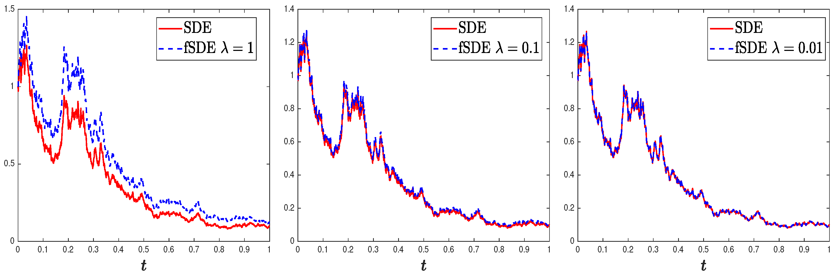
We have performed some numerical expriments to test the correctness of the theoretical results. The numerial scheme is applied for (2). The time interval is assumed $[0,T]=[0,1]$. We discretize time by $t_n=n\Delta t$ with $\Delta t=2^{-10}.$ We choose 1024 sample paths and $f\left(u\right)=\sigma \left(u\right)=-u.$ The initial condition is $u_0=1$ and $\kappa \left(t\right)=t^2$. Then, we plot the solutions in Figure 1. We observe that the FSDE reduces to the classical SDE as the parameter $\lambda$ changes from 1 to 0.

Figure 1. Numerical simulations: classical integer-order SDE (’red line’) and the FSDE (’blue dots’) with $\kappa \left(t\right)=t^2$ for cases (i) left $\lambda =1$, medium $\lambda =0.1$, and right $\lambda =0.001$.

6. Conclusions

We analyzed the solution to the variable-order FSDEs. The moment estimate was also derived. Furthermore, we also analyzed the corresponding inversed problem. Some numerical examples are performed. These investigations will contribute to a deeper understanding of the underlying dynamics and provide novel tools for tackling real-world problems.

References

- Evans, L.C. An Introduction to Stochastic Differential Equations; American Mathematical Society: Providence, RI, USA, 2014. [Google Scholar]
- Klebaner, F.C. Introduction to Stochastic Calculus with Applications; World Scientific Publishing Company: Singapore, 2005. [Google Scholar]
- Kloeden, P.E.; Platen, E. Numerical Solution of Stochastic Differential Equations; Springer: Berlin/Heidelberg, Germany, 1992. [Google Scholar]
- Øksendal, B. Stochastic Differential Equations: An Introduction with Applications; Springer: Berlin/Heidelberg, Germany, 2010. [Google Scholar]
- Shreve, S.E. Stochastic Calculus for Finance II: Continuous-Time Models; Springer Science and Business Media: Berlin/Heidelberg, Germany, 2004. [Google Scholar]
- Zhang, Z.; Karniadakis, G.E. Numerical Methods for Stochastic Partial Differential Equations with White Noise; Springer: Berlin/Heidelberg, Germany, 2017; Volume 196. [Google Scholar]
- Bagley, R.; Torvik, P. A theoretical basis for the application of fractional calculus to viscoelasticity. J. Rheol. 1983, 27, 201–210. [Google Scholar] [CrossRef] [Scilit]
- Mainardi, F. Fractional Calculus and Waves in Linear Viscoelasticity: An Introduction to Mathematical Models; World Scientific: Singapore, 2010. [Google Scholar]
- Weiss, M.; Elsner, M.; Kartberg, F.; Nilsson, T. Anomalous subdiffusion is a measure for cytoplasmic crowding in living cells. Biophys. J. 2004, 87, 3518–3524. [Google Scholar] [CrossRef] [Scilit]
- Diethelm, K. The Analysis of Fractional Differential Equations; Ser. Lecture Notes in Mathematics; Springer: Berlin/Heidelberg, Germany, 2010; Volume 2004. [Google Scholar]
- Metzler, R.; Klafter, J. The random walk’s guide to anomalous diffusion: A fractional dynamics approach. Phys. Rep. 2000, 339, 1–77. [Google Scholar] [CrossRef] [Scilit]
- Podlubny, I. Fractional Differential Equations; Academic Press: Cambridge, MA, USA, 1999. [Google Scholar]
- Lutz, E. Fractional Langevin equation. Phys. Rev. E 2001, 64, 051106. [Google Scholar] [CrossRef] [Scilit] [PubMed]
- Ahmadova, A.; Mahmudov, N. Existence and uniqueness results for a class of fractional stochastic neutral differential equations. Chaos Solitons Fractals 2020, 139, 110253. [Google Scholar] [CrossRef] [Scilit]
- Dai, X.; Bu, W.; Xiao, A. Well-posedness and EM approximations for non-Lipschitz stochastic fractional integro-differential equations. J. Comput. Appl. Math. 2019, 356, 377–390. [Google Scholar] [CrossRef] [Scilit]
- Gunzburger, M.; Li, B.; Wang, J. Sharp convergence rates of time discretization for stochastic time-fractional PDEs subject to additive space-time white noise. Math. Comp. 2019, 88, 1715–1741. [Google Scholar] [CrossRef] [Scilit]
- Shi, K.; Wang, Y. On a stochastic fractional partial differential equation driven by a Lévy space-time white noise. J. Math. Anal. Appl. 2010, 364, 119–129. [Google Scholar] [CrossRef] [Scilit]
- Huang, J.; Huo, Z.; Zhang, J.; Tang, Y. An Euler-Maruyama method and its fast implementation for multiterm fractional stochastic differential equations. Math. Methods Appl. Sci. 2023, 46, 1556–1573. [Google Scholar] [CrossRef] [Scilit]
- Zhao, Y.; Mao, Z.; Guo, L.; Tang, Y.; Karniadakis, G. A spectral method for stochastic fractional PDEs using dynamically-orthogonal/bi-orthogonal decomposition. J. Comput. Phys. 2022, 461, 111213. [Google Scholar] [CrossRef] [Scilit]
- Zhang, J.; Lv, J.; Huang, J.; Tang, Y. A fast Euler-Maruyama method for Riemann-Liouville stochastic fractional nonlinear differential equations. Phys. D 2023, 446, 133685. [Google Scholar] [CrossRef] [Scilit]
- Zhang, J.; Tang, Y.; Huang, J. A fast Euler-Maruyama method for fractional stochastic differential equations. J. Appl. Math. Comput. 2023, 69, 273–291. [Google Scholar] [CrossRef] [Scilit]
- Embrechts, P.; Maejima, M. Selfsimilar Processes; Princeton Series in Applied Mathematics; Princeton University Press: Princeton, NJ, USA, 2002. [Google Scholar]
- Meerschaert, M.M.; Sikorskii, A. Stochastic Models for Fractional Calculus; Series: De Gruyter Studies in Mathematics; De Gruyter: Berlin, Germany, 2011. [Google Scholar]
- Lorenzo, C.F.; Hartley, T.T. Variable order and distributed order fractional operators. Nonlinear Dyn. 2002, 29, 57–98. [Google Scholar] [CrossRef] [Scilit]
- Samko, S.; Ross, B. Integration and differentiation to a variable fractional order. Integral Transform. Spec. Funct. 1993, 1, 277–300. [Google Scholar] [CrossRef] [Scilit]
- Sun, H.; Chen, W.; Chen, Y. Variable-order fractional differential operators in anomalous diffusion modeling. Phys. A Stat. Mech. Its Appl. 2009, 388, 4586–4592. [Google Scholar] [CrossRef] [Scilit]
- Wang, H.; Zheng, X. Wellposedness and regularity of the variable-order time-fractional diffusion equations. J. Math. Anal. Appl. 2019, 475, 1778–1802. [Google Scholar] [CrossRef] [Scilit]
- Zeng, F.; Zhang, Z.; Karniadakis, G. A generalized spectral collocation method with tunable accuracy for variable-order fractional differential equations. SIAM J. Sci. Comput. 2015, 37, A2710–A2732. [Google Scholar] [CrossRef] [Scilit]
- Zhuang, P.; Liu, F.; Anh, V.; Turner, I. Numerical methods for the variable-order fractional advection-diffusion equation with a nonlinear source term. SIAM J. Numer. Anal. 2009, 47, 1760–1781. [Google Scholar] [CrossRef] [Scilit]
- Hatano, Y.; Nakagawa, J.; Wang, S.; Yamamoto, M. Determination of order in fractional diffusion equation. J. Math-for-Ind. 2013, 5A, 51–57. [Google Scholar]
- Janno, J. Determination of the order of fractional derivative and a kernel in an inverse problem for a generalized time fractional diffusion equation. Elect J. Differ. Eqs. 2016, 199, 1–28. [Google Scholar]
- Jin, B.; Rundell, W. An inverse problem for a one-dimensional time-fractional diffusion problem. Inverse Probl. 2012, 28, 75010–75028. [Google Scholar] [CrossRef] [Scilit]
- Kian, Y.; Oksanen, L.; Soccorsi, E.; Yamamoto, M. Global uniqueness in an inverse problem for time fractional diffusion equations. J. Diff. Eqs. 2018, 264, 1146–1170. [Google Scholar] [CrossRef] [Scilit]
- Li, Z.; Yamamoto, M. Uniqueness for inverse problems of determining orders of multi-term time-fractional derivatives of diffusion equation. Appl. Anal. 2015, 94, 570–579. [Google Scholar] [CrossRef] [Scilit]
- Liang, J.; Chen, Y.; Vinagre, B.; Podlubny, I. Identifying diffusion-wave constant, fractional order and boundary profile of a time-fractional diffusion-wave equation from noisy boundary measurements. In Fractional Differentiation and Its Applications; Mehauté, A., Tenreiro, J., Trigeassou, J., Sabatier, J., Eds.; Ubooks: Mossautal, Germany, 2005; pp. 517–532. [Google Scholar]
- Liu, J.; Yamamoto, M. A backward problem for the time-fractional diffusion equation. Appl. Anal. 2010, 89, 1769–1788. [Google Scholar] [CrossRef] [Scilit]
- Xu, X.; Cheng, J.; Yamamoto, M. Carleman estimate for a fractional diffusion equation with half order and application. Appl. Anal. 2011, 90, 1355–1371. [Google Scholar] [CrossRef] [Scilit]
- Zheng, G.; Wei, T. A new regularization method for the time fractional inverse advection-dispersion problem. SIAM J. Numer. Anal. 2011, 49, 1972–1990. [Google Scholar] [CrossRef] [Scilit]
- Li, G.; Zhang, D.; Jia, X.; Yamamoto, M. Simultaneous inversion for the space-dependent diffusion coefficient and the fractional order in the time-fractional diffusion equation. Inverse Probl. 2013, 29, 065014. [Google Scholar] [CrossRef] [Scilit]
- Li, Z.; Huang, X.; Yamamoto, M. A stability result for the determination of order in time-fractional diffusion equations. J. Inv. Ill-Posed Prob. 2019, 28, 379–388. [Google Scholar] [CrossRef] [Scilit]
- Kian, Y.; Soccorsi, E.; Yamamoto, M. On time-fractional diffusion equations with space-dependent variable order. Ann. Henri Poincaré 2018, 19, 3855–3881. [Google Scholar] [CrossRef] [Scilit]
- Mao, Z.; Li, Z.; Karniadakis, G.E. Nonlocal flocking dynamics: Learning the fractional order of PDEs from particle simulations. Commun. Appl. Math. Comp. 2019, 1, 597–619. [Google Scholar] [CrossRef] [Scilit]
- Mehta, P.; Pang, G.; Song, F.; Karniadakis, G.E. Discovering a universal variable-order fractional model for turbulent Couette flow using a physics-informed neural network. Fract. Calc. Appl. Anal. 2019, 22, 1675–1688. [Google Scholar] [CrossRef] [Scilit]
- Zheng, X.; Cheng, J.; Wang, H. Uniqueness of determining the variable fractional order in variable-order time-fractional diffusion equations. Inverse Probl. 2019, 35, 125002. [Google Scholar] [CrossRef] [Scilit]
- Adams, R.A.; Fournier, J.J.F. Sobolev Spaces; Elsevier: San Diego, CA, USA, 2003. [Google Scholar]
- Brunner, H. Collocation Methods for Volterra Integral and Related Functional Differential Equations; Cambridge University Press: Cambridge, UK, 2004. [Google Scholar]
- Kilbas, A.; Srivastava, H.; Trujillo, J. Theory and Applications of Fractional Differential Equations; Elsevier: Amsterdam, The Netherlands, 2006; Volume 204. [Google Scholar]
- Le Gall, J.F. Brownian Motion, Martingales, and Stochastic Calculus; Springer: Berlin/Heidelberg, Germany, 2016. [Google Scholar]
- Zheng, X.; Zhang, Z.; Wang, H. Analysis of a nonlinear variable-order fractional stochastic differential equation. Appl. Math. Lett. 2020, 107, 106461. [Google Scholar] [CrossRef] [Scilit]
Disclaimer/Publisher’s Note: The statements, opinions and data contained in all publications are solely those of the individual author(s) and contributor(s) and not of MDPI and/or the editor(s). MDPI and/or the editor(s) disclaim responsibility for any injury to people or property resulting from any ideas, methods, instructions or products referred to in the content. |
© 2023 by the authors. Licensee MDPI, Basel, Switzerland. This article is an open access article distributed under the terms and conditions of the Creative Commons Attribution (CC BY) license (https://creativecommons.org/licenses/by/4.0/).