Efficient Inverse Fractional Neural Network-Based Simultaneous Schemes for Nonlinear Engineering Applications

Abstract

Finding all the roots of a nonlinear equation is an important and difficult task that arises naturally in numerous scientific and engineering applications. Sequential iterative algorithms frequently use a deflating strategy to compute all the roots of the nonlinear equation, as rounding errors have the potential to produce inaccurate results. On the other hand, simultaneous iterative parallel techniques require an accurate initial estimation of the roots to converge effectively. In this paper, we propose a new class of global neural network-based root-finding algorithms for locating real and complex polynomial roots, which exploits the ability of machine learning techniques to learn from data and make accurate predictions. The approximations computed by the neural network are used to initialize two efficient fractional Caputo-inverse simultaneous algorithms of convergence orders $\varsigma +2$ and $2\varsigma +4$, respectively. The results of our numerical experiments on selected engineering applications show that the new inverse parallel fractional schemes have the potential to outperform other state-of-the-art nonlinear root-finding methods in terms of both accuracy and elapsed solution time.

1. Introduction

Determining the roots of nonlinear equations of the form

$$f\left(\upsilon \right)=0,$$

(1)

is among the oldest problems in science and engineering, dating back to at least 2000 BC, when the Babylonians discovered a general solution to quadratic equations. In 1079, Omer Khayyams developed a geometric method for solving cubic equations. In 1545, in his book Ars Magna, Girolomo Cardano published a universal solution to a cubic polynomial equation. Cordano was one of the first authors to use complex numbers, but only to derive real solutions to generic polynomials. Niel Hernor Abel [1] proved Abel’s Impossibility theorem “There is no solution in radical to general polynomial with arbitrary coefficient of degree five or higher” in 1824. The fact established in the 17th century that every generic polynomial equation of positive degree has a solution, possibly non-real, was completely demonstrated at the beginning of the 19th century as the “Fundamental theorem of algebra” [2].

From the beginning of the 16th century to the end of the 19th century, one of the main problems in algebra was to find a formula that computed the solution of a generic polynomial with arbitrary coefficients of degree equal to or greater than five. Because there are no analytical or implicit methods for solving this problem, we must rely on numerical techniques to approximate the roots of higher-degree polynomials. These numerical algorithms can be further divided into two categories: those that estimate one polynomial root at a time and those that approximate all polynomial roots simultaneously. Work in this area began in 1970, with the primary goal of developing numerical iterative techniques that could locate polynomial roots on contemporary, state-of-the-art computers with optimal speed and efficiency [3]. Iterative approaches are currently used to find polynomial roots in a variety of disciplines. In signal processing, polynomial roots are the frequencies of signals representing sounds, images, and movies. In control theory, they characterize the behavior of control systems and can be utilized to enhance system stability or performance. The prices of options and futures contracts are determined by estimating the roots of (1); therefore, it is critical to compute them accurately so that they can be priced precisely.

In recent years, many iterative techniques for estimating the roots of nonlinear equations have been proposed. These methods use several quadrature rules, interpolation techniques, error analysis, and other techniques to improve the convergence order of previously known single-root-finding procedures [4,5,6]. In this paper, we will focus on iterative approaches for solving single-variable nonlinear equations one root at a time. However, we will generalize these methods to locate all distinct roots of nonlinear equations simultaneously. A sequential approach for finding all the zeros in a polynomial necessitates repeated deflation, which can produce significantly inaccurate results due to rounding errors propagating in finite-precision floating-point arithmetic. As a result, we employ more precise, efficient, and stable simultaneous approaches. The literature is vast and dates back to 1891, when Weierstrass introduced the single-step derivative-free simultaneous method [7] for finding all polynomial roots, which was later rediscovered by Kerner [8], Durand [9], Dochev [10], and Presic [11]. Gauss–Seidal [12] and Petkovic et al. [13] introduced the second-order method for approximating all roots simultaneously; Börsch–Supan [14] and Mir [15] presented the third-order method; Provinic et al [16] introduced the fourth-order method; and Zhang et al [17] the fifth-order method. Additional enhancements in efficiency were demonstrated by Ehlirch in [18] and Milovanovic et al. in [19]; Nourein proposed a fourth-order method in [20]; and Petkovic et al. a six-order simultaneous method with derivatives in [21]. Former [22] introduced the percentage efficacy of simultaneous methods in 2014. Later, in 2015, Proinov et al. [23] presented a general convergence theorem for simultaneous methods and a description of the application of the Weierstrass root approximating methodology. In 2016, Nedzibove [24] developed a modified version of the Weierstrass method, and in 2020, Marcheva et al. [25] presented the local convergence theorem. Shams et al. [26,27] presented the computational efficiency ratios for the simultaneous approach on initial vectors to locate all polynomial roots in 2020, as well as the global convergence in 2022 [28]. Additional advancements in the field can be found in [29,30,31,32,33] and the references therein.

The primary goal of this study is to develop Caputo-type fractional inverse simultaneous schemes that are more robust, stable, computationally inexpensive, and CPU-efficient compared to existing methods. The theory and analysis of inverse fractional parallel numerical Caputo-type schemes, as well as their practical implementation utilizing artificial neural networks (ANNs) for approximating all roots of (1), are also thoroughly examined. Simultaneous schemes, Caputo-type fractional inverse simultaneous schemes, and simultaneous schemes based on artificial neural networks are all discussed and compared in depth. The main contributions of this study are as follows:

• Two novel fractional inverse simultaneous Caputo-type methods are introduced in order to locate all the roots of (1).
• A local convergence analysis is presented for the parallel fractional inverse numerical schemes that are proposed.
• A rigorous complexity analysis is provided to demonstrate the increased efficiency of the new method.
• The Levenberg–Marquardt Algorithm is utilized to compute all of the roots using ANNs.
• The global convergence behavior of the proposed inverse fractional parallel root-finding method with random initial estimate values is illustrated.
• The efficiency and stability of the new method are numerically assessed using dynamical planes.
• The general applicability of the method for various nonlinear engineering problems is thoroughly studied using different stopping criteria and random initial guesses.

To the best of our knowledge, this contribution is novel. A review of the existing body of literature indicates that research on fractional parallel numerical methods for simultaneously locating all roots of (1) is extremely limited. This paper is organized as follows. In Section 2, a number of fundamental definitions are given. The construction, analysis, and assessment of inverse fractional algorithms are covered in Section 3. A comparison is made between the artificial neural network aspects of recently developed parallel methods and those of existing schemes in Section 4. A cost analysis of classical and fractional parallel schemes is detailed in Section 5. A dynamical analysis of global convergence is presented in Section 6. In order to evaluate the newly developed techniques in comparison to the parallel computer algorithms that are currently documented in the literature, Section 7 solves a number of nonlinear engineering applications and reports on the numerical results. The global convergence behavior of the inverse parallel scheme is also compared to that of a simultaneous neural network-based method in this section. Finally, some conclusions arising from this work are drawn in Section 8.

2. Preliminaries

Despite the fact that with the exception of the Caputo derivative, none of the fractional-type derivatives satisfy the fractional calculus conditions, $\left[{⅁}^{\varsigma }\right]\left(1\right)=0$, if $\varsigma$ is not a natural number, in this section we discuss some basic concepts of fractional calculus, as well as the fractional iterative scheme for solving (1) using Caputo-type derivatives.

The Gamma function is described as follows [34]:

$$\lceil \left(\upsilon \right)=\underset{0}{\overset{+\infty }{\int }}{u}^{\upsilon -1}{e}^{-u}du,$$

(2)

where $\upsilon >0.$ With $\lceil \left(1\right)=1$ and $\lceil (\sigma +1)=\sigma !$, where $\sigma \in N$, Gamma is a generalization of the factorial function.

For

$$f:\mathbb{R}\to \mathbb{R},f\in {\mathbb{C}}^{+\infty }\left(\left[\varsigma ,\upsilon \right]\right),-\infty <\varsigma <\upsilon <+\infty ,\varsigma \ge 0,m=\left[\varsigma \right]+1,$$

order $\varsigma$’s Caputo fractional derivative is defined as [35]:

$$\left[{}_C{⅁}_{{\varsigma }_1}^{\varsigma }\right]f\left(\upsilon \right)=\left\{\begin{array}{c}\frac{1}{\lceil (m-\varsigma )}\underset{0}{\overset{\upsilon }{\int }}\frac{d^m}{d{t}^m}f\left(t\right)\frac{1}{{\left(\upsilon -t\right)}^{\varsigma -m+1}}dt,\varsigma \in N,\\ \frac{d^{m-1}}{d{t}^m-1}f\left(\upsilon \right),\varsigma =m-1\in N\cup \left\{0\right\},\end{array}\right.$$

(3)

where $\lceil \left(\upsilon \right)$ is a gamma function with $\upsilon >0.$

Theorem 1

(Generalized Taylor Formula [36]). The generalized Taylor theorem of fractional order is a powerful mathematical tool that extends the applicability of Taylor series approximations to fractional-order functions that model and describe a wide range of complex phenomena in a variety of scientific and engineering domains, including signal processing, control theory, biomedical engineering, image processing, chaos theory, economic and financial modeling, and many more.

Suppose $\left[{}_C{⅁}_{{\varsigma }_1}^{\gamma \vartheta }\right]f\left(\upsilon \right)\in C\left(\left[{\varsigma }_1,{\varsigma }_2\right]\right)$ for $\gamma =1,\dots ,\sigma +1$, where $\varsigma \in \left(0,1\right]$. Then,

$$f\left(\upsilon \right)=\sum _{i=0}^{\sigma }\left[{}_C{⅁}_{{\varsigma }_1}^{i\varsigma }\right]f\left({\varsigma }_1\right)\frac{{\left(\upsilon -{\varsigma }_1\right)}^{i\varsigma }}{\lceil (i\varsigma +1)}+\left[{}_C{⅁}_{{\varsigma }_1}^{\left(\sigma +1\right)\varsigma }\right]f\left(\zeta \right)\frac{{\left(\upsilon -{\varsigma }_1\right)}^{\left(\sigma +1\right)\varsigma }}{\lceil (\left(\sigma +1\right)\varsigma +1)},$$

(4)

and ${\varsigma }_1\le \zeta \le \upsilon ,\forall \upsilon \in \left({\varsigma }_1,{\varsigma }_2\right]$ and $\left[{}_C{⅁}_{{\varsigma }_1}^{n\ast \varsigma }\right]=\left[{}_C{⅁}_{{\varsigma }_1}^{\varsigma }\right].\left[{}_C{⅁}_{{\varsigma }_1}^{\varsigma }\right]\dots \left[{}_C{⅁}_{{\varsigma }_1}^{\varsigma }\right]$ (n-times). In terms of the Caputo-type Taylor development of $f\left(\upsilon \right)$ around ${\varsigma }_1=\zeta$, then

$$f\left(\upsilon \right)=\frac{\left[{}_C{⅁}_{\zeta }^{\varsigma }\right]f\left(\zeta \right)}{\lceil (\varsigma +1)}{\left(\upsilon -\zeta \right)}^{\varsigma }+\frac{\left[{}_C{⅁}_{\zeta }^{2\varsigma }\right]f\left(\zeta \right)}{\lceil (2\varsigma +1)}{\left(\upsilon -\zeta \right)}^{2\varsigma }+O{\left(\upsilon -\zeta \right)}^{3\varsigma }.$$

(5)

Factoring $\frac{\left[{}_C{⅁}_{\zeta }^{\varsigma }\right]f\left(\zeta \right)}{\lceil (\varsigma +1)}$, we have:

$$f\left(\upsilon \right)=\frac{\left[{}_C{⅁}_{\zeta }^{\varsigma }\right]f\left(\zeta \right)}{\lceil (\varsigma +1)}\left[{\left(\upsilon -\zeta \right)}^{\varsigma }+C_2{\left(\upsilon -\zeta \right)}^{2\varsigma }\right]+O{\left(\upsilon -\zeta \right)}^{3\varsigma },$$

(6)

where

$$C_{\gamma }=\frac{\lceil (\varsigma +1)}{\lceil (\gamma \varsigma +1)}\frac{\left[{}_C{⅁}_{\zeta }^{\gamma \varsigma }\right]f\left(\zeta \right)}{\left[{}_C{⅁}_{\zeta }^{\varsigma }\right]f\left(\zeta \right)},\gamma =2,3,\dots$$

(7)

The corresponding Caputo-type fractional derivative of $f\left(\upsilon \right)$ around ζ is

$$\left[{}_C{⅁}_{\zeta }^{\varsigma }\right]f\left(\upsilon \right)=\frac{\left[{}_C{⅁}_{\zeta }^{\varsigma }\right]f\left(\zeta \right)}{\lceil (\varsigma +1)}\left[\lceil (\varsigma +1)+\frac{\lceil (2\varsigma +1)}{\lceil (\varsigma +1)}{C}_2{\left(\upsilon -\zeta \right)}^{\varsigma }\right]+O{\left(\upsilon -\zeta \right)}^{2\varsigma }.$$

(8)

3. Construction of Inverse Fractional Parallel Schemes

Numerical methods for solving nonlinear equations are essential tools for a wide range of problems. They do, however, have trade-offs, such as the necessity for initial guesses, convergence issues, and parameter sensitivity. To produce accurate and efficient answers, the method used should be carefully assessed depending on the specific characteristics of the problem. The Newton–Raphson method,

$$y^{\left(\sigma \right)}={\upsilon }^{\left(\sigma \right)}-\frac{f\left({\upsilon }^{\left(\sigma \right)}\right)}{f^{{}^{\prime }}\left({\upsilon }^{\left(\sigma \right)}\right)},(i=1,2,\dots ),f^{{}^{\prime }}\left({\upsilon }^{\left(\sigma \right)}\right)\ne 0,$$

(9)

is a widely used algorithm for locating a single root of (1). If $f^{{}^{\prime }}\left({\upsilon }^{\left(\sigma \right)}\right)\to 0$, the method becomes unstable. As a result, we consider an alternate technique based on fractional-order iterative algorithms in this paper.

The fractional Newton approach using different fractional derivatives is discussed by Akgül et al. [37], Torres-Hernandez et al. [38], Gajori et al. [39], and Kumar et al. [40]. Candelario et al. [41] proposed the following Caputo-type fractional variant of the classical Newton method (FNN):

$${\upsilon }^{(\sigma +1)}={\upsilon }^{\left(\sigma \right)}-{\left(\lceil (\varsigma +1)\frac{f\left({\upsilon }^{\left(\sigma \right)}\right)}{\left[{}_C{⅁}_{{\varsigma }_1}^{\varsigma }\right]f\left({\upsilon }^{\left(\sigma \right)}\right)}\right)}^{1/\varsigma },$$

(10)

where $\left[{}_C{⅁}_{{\varsigma }_1}^{\varsigma }\right]f\left({\upsilon }^{\left(\sigma \right)}\right)\approx \left[{}_C{⅁}_{\zeta }^{\varsigma }\right]f\left(\zeta \right)$ for any $\varsigma \in \mathbb{R}.$ The following error equation is satisfied by the order of convergence of the fractional Newton method, which is $\varsigma +1,$

$$e^{(\sigma +1)}=\left(\frac{{\lceil (2\varsigma +1)-\lceil }^2(\varsigma +1)}{\varsigma {\lceil }^2(\varsigma +1)}\right)C_2{e}_i^{\varsigma +1}+O\left(e_i^{2\varsigma +1}\right),$$

(11)

where $e^{(\sigma +1)}={\upsilon }^{(\sigma +1)}-\zeta$ and $e^{\left(\sigma \right)}={\upsilon }^{\left(\sigma \right)}-\zeta$ and $C_{\gamma }=\left(\frac{\lceil (\varsigma +1)}{\lceil (\gamma \varsigma +1)}\right)\left(\frac{\left[{}_C{⅁}_{\zeta }^{\gamma \varsigma }\right]f\left(\zeta \right)}{\left[{}_C{⅁}_{\zeta }^{\varsigma }\right]f\left(\zeta \right)}\right),\gamma =2,3,\dots$

Candelario et al. [41] proposed another fractional numerical scheme for calculating simple roots of (1) as:

$$\left\{\begin{array}{c}{y}^{\left(\sigma \right)}={\upsilon }^{\left(\sigma \right)}-{\left(\lceil (\varsigma +1)\frac{f\left({\upsilon }^{\left(\sigma \right)}\right)}{\left[{}_C{⅁}_{{\varsigma }_1}^{\varsigma }\right]f\left({\upsilon }^{\left(\sigma \right)}\right)}\right)}^{1/\varsigma },\\ z^{\left(\sigma \right)}=y^{\left(\sigma \right)}-{\left(\lceil (\varsigma +1)\frac{f\left(y^{\left(\sigma \right)}\right)}{\left[{}_C{⅁}_{{\varsigma }_1}^{\varsigma }\right]f\left({\upsilon }^{\left(\sigma \right)}\right)}\right)}^{1/\varsigma }.\end{array}\right.$$

(12)

The order of convergence of the numerical scheme is $2\varsigma +1$, and the associated error equation is:

$$e^{(\sigma +1)}=\left(\frac{-\lceil (2\varsigma +1)-\lceil (\varsigma +1)}{{\varsigma }^2{\ast \lceil }^2(\varsigma +1)}\right)G\ast C_2^2{e}_i^{2\varsigma +1}+O\left(e_i^{{\varsigma }^2+2\varsigma +1}\right),$$

being ${\varsigma }^2+2\varsigma +1<3\varsigma +1$$\forall \varsigma \in \left(0,1\right]$, $e^{(\sigma +1)}=z^{\left(\sigma \right)}-\zeta$ and $G=\frac{{\lceil }^2(\varsigma +1)-\lceil (2\varsigma +1)}{{\lceil }^2(\varsigma +1)}.$

There have recently been numerous studies on iterative root-finding algorithms that can precisely approximate one root of (1) at a time [42,43,44,45]. The class of fractional numerical schemes is particularly sensitive to the choice of the initial guesses; if we do not choose a suitable initial guess sufficiently close to a root of (1), the method becomes unstable and may not converge. As a result, we explore numerical schemes with global convergence properties, i.e., parallel numerical schemes for simultaneously finding all roots of (1).

3.1. Construction of Inverse Fractional Parallel Scheme of Order $\varsigma +2$

The German mathematician Karl Weierstrass (1815–1897) developed the Weierstrass (WDKI) method for finding roots of (1), which is based on the following quadratically convergent iterative scheme [46]:

$$u_i^{\left(\sigma \right)}={\upsilon }_i^{\left(\sigma \right)}-\frac{f\left({\upsilon }_i^{\left(\sigma \right)}\right)}{\underset{\stackrel{j=1}{j\ne i}}{\stackrel{n}{\Pi }}({\upsilon }_i^{\left(\sigma \right)}-{\upsilon }_j^{\left(\sigma \right)})}.$$

(13)

In order to reduce the computational costs and enhance the convergence rates, we investigate inverse simultaneous methods [47]. The inverse simultaneous scheme applied to (1) is given as [48]:

$$u_i^{\left(\sigma \right)}=\frac{{\left({\upsilon }_i^{\left(\sigma \right)}\right)}^2\ast \left(\underset{\stackrel{j=1}{j\ne i}}{\stackrel{n}{\Pi }}({\upsilon }_i^{\left(\sigma \right)}-{\upsilon }_j^{\left(\sigma \right)})\right)}{{\upsilon }_i^{\left(\sigma \right)}\underset{\stackrel{j=1}{j\ne i}}{\ast \stackrel{n}{\Pi }}({\upsilon }_i^{\left(\sigma \right)}-{\upsilon }_j^{\left(\sigma \right)})+f\left({\upsilon }_i^{\left(\sigma \right)}\right)}.$$

(14)

Method (13) can also be expressed as:

$$u_i^{\left(\sigma \right)}{=}_i^{\left(\sigma \right)}-\frac{\left({\upsilon }_i^{\left(\sigma \right)}\right)\ast f\left({\upsilon }_i^{\left(\sigma \right)}\right)}{{\upsilon }_i^{\left(\sigma \right)}\underset{\stackrel{j=1}{j\ne i}}{\ast \stackrel{n}{\Pi }}({\upsilon }_i^{\left(\sigma \right)}-{\upsilon }_j^{\left(\sigma \right)})+f\left({\upsilon }_i^{\left(\sigma \right)}\right)},$$

(15)

replacing ${\upsilon }_j^{\left(\sigma \right)}$ with $y_j^{\ast \left(\sigma \right)}$ in (14). As a result, our new inverse fractional simultaneous scheme (FINS${}_{\varsigma }$) is established as follows:

$$u_i^{\left(\sigma \right)}=\frac{{\left({\upsilon }_i^{\left(\sigma \right)}\right)}^2\ast \left(\underset{\stackrel{j=1}{j\ne i}}{\stackrel{n}{\Pi }}\left({\upsilon }_i^{\left(\sigma \right)}-y_j^{\ast \left(\sigma \right)}\right)\right)}{{\upsilon }_i^{\left(\sigma \right)}\ast \left(\underset{\stackrel{j=1}{j\ne i}}{\stackrel{n}{\Pi }}\left({\upsilon }_i^{\left(\sigma \right)}-y_j^{\ast \left(\sigma \right)}\right)\right)+f\left({\upsilon }_i^{\left(\sigma \right)}\right)},$$

(16)

where $y_j^{\ast \left(\sigma \right)}={\upsilon }_j^{\left(\sigma \right)}-{\left(\lceil (\varsigma +1)\frac{f\left({\upsilon }_j^{\left(\sigma \right)}\right)}{\left[{}_C{⅁}_{{\varsigma }_1}^{\varsigma }\right]f\left({\upsilon }_j^{\left(\sigma \right)}\right)}\right)}^{1/\varsigma }.$ Method (16) can also be written as:

$$u_i^{\left(\sigma \right)}=\frac{{\left({\upsilon }_i^{\left(\sigma \right)}\right)}^2\ast \left(\underset{\stackrel{j=1}{j\ne i}}{\stackrel{n}{\Pi }}\left({\upsilon }_i^{\left(\sigma \right)}-{\upsilon }_j^{\left(\sigma \right)}-{\left(\lceil (\varsigma +1)\frac{f\left({\upsilon }_j^{\left(\sigma \right)}\right)}{\left[{}_C{⅁}_{{\varsigma }_1}^{\varsigma }\right]f\left({\upsilon }_j^{\left(\sigma \right)}\right)}\right)}^{1/\varsigma }\right)\right)}{{\upsilon }_i^{\left(\sigma \right)}\ast \left(\underset{\stackrel{j=1}{j\ne i}}{\stackrel{n}{\Pi }}\left({\upsilon }_i^{\left(\sigma \right)}-{\upsilon }_j^{\left(\sigma \right)}-{\left(\lceil (\varsigma +1)\frac{f\left({\upsilon }_j^{\left(\sigma \right)}\right)}{\left[{}_C{⅁}_{{\varsigma }_1}^{\varsigma }\right]f\left({\upsilon }_j^{\left(\sigma \right)}\right)}\right)}^{1/\varsigma }\right)\right)+f\left({\upsilon }_i^{\left(\sigma \right)}\right)}.$$

(17)

The newly developed inverse fractional-order inverse parallel schemes outperform other current approaches in the literature in terms of convergence order, as proven by the following convergence analysis.

Convergence Framework

The following theorem examines the convergence order of FINS${}_{\varsigma }$.

Theorem 2.

Let ${\zeta }_1,\dots ,{\zeta }_{\sigma }$ be a simple zero of (1), and for a sufficiently close initial distinct estimation, ${\upsilon }_1^{\left(0\right)},\dots ,{\upsilon }_{\sigma }^{\left(0\right)}$, of the roots, FINS${}_{\varsigma }$ has a convergence order of $\varsigma +2$.

Proof. 

Let ${ϵ}_i={\upsilon }_i^{\left(\sigma \right)}-{\zeta }_i,{ϵ}_i^{\prime }=u_i^{\left(\sigma \right)}-{\zeta }_i$ be the errors in ${\upsilon }_i^{\left(\sigma \right)},$ and$u_i^{\left(\sigma \right)}$, respectively. Then,

$$u_i^{\left(\sigma \right)}-{\zeta }_i={\upsilon }_i^{\left(\sigma \right)}-{\zeta }_i-\frac{{\upsilon }_i^{\left(\sigma \right)}f\left({\upsilon }_i^{\left(\sigma \right)}\right)}{{\upsilon }_i^{\left(\sigma \right)}\left(\underset{\stackrel{j=1}{j\ne i}}{\stackrel{\sigma }{\Pi }}({\upsilon }_i^{\left(\sigma \right)}-{\stackrel{\ast }{y}}_j^{\left(\sigma \right)})\right)+f\left({\upsilon }_i^{\left(\sigma \right)}\right)}.$$

(18)

Thus, we obtain

$${ϵ}_i^{\prime }={ϵ}_i\left[1-\frac{{\displaystyle \prod _{\underset{j=1}{j\ne i}}^n}\frac{({\upsilon }_i^{\left(\sigma \right)}-{\zeta }_j)}{({\upsilon }_i^{\left(\sigma \right)}-{\stackrel{\ast }{y}}_j^{\left(\sigma \right)})}}{1+\frac{f\left({\upsilon }_i^{\left(\sigma \right)}\right)}{\underset{\stackrel{j=1}{j\ne i}}{\stackrel{n}{\Pi }}({\upsilon }_i^{\left(\sigma \right)}-{\stackrel{\ast }{y}}_j^{\left(\sigma \right)})}}\right]={ϵ}_i\left[\frac{1-{\displaystyle \prod _{\underset{j=1}{j\ne i}}^n}\frac{({\upsilon }_i^{\left(\sigma \right)}-{\zeta }_j)}{({\upsilon }_i^{\left(\sigma \right)}-{\stackrel{\ast }{y}}_j^{\left(\sigma \right)})}+\frac{f\left({\upsilon }_i^{\left(\sigma \right)}\right)}{\underset{\stackrel{j=1}{j\ne i}}{\stackrel{n}{\Pi }}({\upsilon }_i^{\left(\sigma \right)}-{\stackrel{\ast }{y}}_j^{\left(\sigma \right)})}}{1+\frac{f\left({\upsilon }_i^{\left(\sigma \right)}\right)}{\underset{\stackrel{j=1}{j\ne i}}{\stackrel{n}{\Pi }}({\upsilon }_i^{\left(\sigma \right)}-{\stackrel{\ast }{y}}_j^{\left(\sigma \right)})}}\right].$$

(19)

Using the expression ${\displaystyle \prod _{\underset{j=1}{j\ne i}}^n}\frac{({\upsilon }_i^{\left(\sigma \right)}-{\zeta }_j)}{({\upsilon }_i^{\left(\sigma \right)}-{\stackrel{\ast }{y}}_j^{\left(\sigma \right)})}-1={\displaystyle \sum _{k\ne i}^n}\frac{{ϵ}_k^{\varsigma +1}}{{\upsilon }_i^{\left(\sigma \right)}-{\upsilon }_k^{\left(\sigma \right)}}{\displaystyle \prod _{j\ne i}^{k-1}}\frac{({\upsilon }_i^{\left(\sigma \right)}-{\zeta }_k)}{({\upsilon }_i^{\left(\sigma \right)}-{\stackrel{\ast }{y}}_j^{\left(\sigma \right)})}$ [49] in (19), we have:

$${ϵ}_i^{\prime }={ϵ}_i\left[\frac{\frac{{ϵ}_i^{\varsigma +1}}{{\upsilon }_i^{\left(\sigma \right)}}{\displaystyle \prod _{\underset{j=1}{j\ne i}}^n}\frac{({\upsilon }_i^{\left(\sigma \right)}-{\zeta }_j)}{({\upsilon }_i^{\left(\sigma \right)}-{\stackrel{\ast }{y}}_j^{\left(\sigma \right)})}-{\displaystyle \sum _{k\ne i}^n}\frac{{ϵ}_k^{\varsigma +1}}{{\upsilon }_i^{\left(\sigma \right)}-{\stackrel{\ast }{y}}_k^{\left(\sigma \right)}}{\displaystyle \prod _{j\ne i}^{k-1}}\frac{({\upsilon }_i^{\left(\sigma \right)}-{\zeta }_k)}{({\upsilon }_i^{\left(\sigma \right)}-{\stackrel{\ast }{y}}_j^{\left(\sigma \right)})}}{1+\frac{{ϵ}_k}{{\upsilon }_i^{\left(\sigma \right)}}{\displaystyle \prod _{\underset{j=1}{j\ne i}}^n}\frac{({\upsilon }_i^{\left(\sigma \right)}-{\zeta }_j)}{({\upsilon }_i^{\left(\sigma \right)}-{\stackrel{\ast }{y}}_j^{\left(\sigma \right)})}}\right].$$

(20)

If we assume that all errors are of the same order, i.e., $\left|{ϵ}_i\right|=\left|{ϵ}_k\right|=O\left(\left|ϵ\right|\right),$ then,

$${ϵ}_i^{\prime }={\left|ϵ\right|}^{\varsigma +2}\left[\frac{\frac{1}{{\upsilon }_i}{\displaystyle \prod _{\underset{j=1}{j\ne i}}^n}\frac{({\upsilon }_i^{\left(\sigma \right)}-{\zeta }_j)}{({\upsilon }_i^{\left(\sigma \right)}-{\stackrel{\ast }{y}}_j^{\left(\sigma \right)})}-{\displaystyle \sum _{k\ne i}^n}\frac{1}{{\upsilon }_i^{\left(\sigma \right)}-y_{\sigma }}{\displaystyle \prod _{j\ne i}^{k-1}}\frac{({\upsilon }_i^{\left(\sigma \right)}-{\zeta }_k)}{({\upsilon }_i^{\left(\sigma \right)}-{\stackrel{\ast }{y}}_j^{\left(\sigma \right)})}}{1+\frac{{ϵ}_k}{{\upsilon }_i^{\left(\sigma \right)}}{\displaystyle \prod _{\underset{j=1}{j\ne i}}^n}\frac{({\upsilon }_i^{\left(\sigma \right)}-{\zeta }_j)}{({\upsilon }_i^{\left(\sigma \right)}-{\stackrel{\ast }{y}}_j^{\left(\sigma \right)})}}\right]=O\left({\left|ϵ\right|}^{\varsigma +2}\right).$$

(21)

Hence, the theorem is proved.    □

3.2. Construction of Inverse Fractional Parallel Scheme of Order $2\varsigma +4$

Consider the two-step Weierstrass method [50] with fourth-order convergence, locally defined as:

$$z_i^{\left(\sigma \right)}=u_i^{\left(\sigma \right)}-\frac{f\left(u_i^{\left(\sigma \right)}\right)}{\underset{\stackrel{j=1}{j\ne i}}{\stackrel{n}{\Pi }}(u_i^{\left(\sigma \right)}-u_j^{\left(\sigma \right)})},$$

(22)

where $u_i^{\left(\sigma \right)}={\upsilon }_i^{\left(\sigma \right)}-\frac{f\left({\upsilon }_i^{\left(\sigma \right)}\right)}{\underset{\stackrel{j=1}{j\ne i}}{\stackrel{n}{\Pi }}({\upsilon }_i^{\left(\sigma \right)}-{\upsilon }_j^{\left(\sigma \right)})},$ and the two-step inverse Weierstrass method [51] with fourth-order convergence, locally (IWDKI) defined as:

$$z_i^{\left(\sigma \right)}=\frac{{\left(u_i^{\left(\sigma \right)}\right)}^2\ast \left(\underset{\stackrel{j=1}{j\ne i}}{\stackrel{n}{\Pi }}(u_i^{\left(\sigma \right)}-u_j^{\left(\sigma \right)})\right)}{u_i^{\left(\sigma \right)}\ast \left(\underset{\stackrel{j=1}{j\ne i}}{\stackrel{n}{\Pi }}(u_i^{\left(\sigma \right)}-u_j^{\left(\sigma \right)})\right)+f\left(u_i^{\left(\sigma \right)}\right)},$$

(23)

where $u_i^{\left(\sigma \right)}=\frac{{\left({\upsilon }_i^{\left(\sigma \right)}\right)}^2\ast \left(\underset{\stackrel{j=1}{j\ne i}}{\stackrel{n}{\Pi }}({\upsilon }_i^{\left(\sigma \right)}-{\upsilon }_j^{\left(\sigma \right)})\right)}{{\upsilon }_i^{\left(\sigma \right)}\underset{\stackrel{j=1}{j\ne i}}{\ast \stackrel{n}{\Pi }}({\upsilon }_i^{\left(\sigma \right)}-{\upsilon }_j^{\left(\sigma \right)})+f\left({\upsilon }_i^{\left(\sigma \right)}\right)}.$

Method (23) can also be written as:

$$\left\{\begin{array}{c}{u}_i^{\left(\sigma \right)}={\upsilon }_i^{\left(\sigma \right)}-\frac{\left({\upsilon }_i^{\left(\sigma \right)}\right)\ast f\left({\upsilon }_i^{\left(\sigma \right)}\right)}{{\upsilon }_i^{\left(\sigma \right)}\ast \left(\underset{\stackrel{j=1}{j\ne i}}{\stackrel{n}{\Pi }}({\upsilon }_i^{\left(\sigma \right)}-{\stackrel{\ast }{y}}_j^{\left(\sigma \right)})\right)+f\left({\upsilon }_i^{\left(\sigma \right)}\right)},\\ z_i^{\left(\sigma \right)}=u_i^{\left(\sigma \right)}-\frac{\left(u_i^{\left(\sigma \right)}\right)\ast f\left(u_i^{\left(\sigma \right)}\right)}{u_i^{\left(\sigma \right)}\ast \left(\underset{\stackrel{j=1}{j\ne i}}{\stackrel{n}{\Pi }}(u_i^{\left(\sigma \right)}-u_j^{\left(\sigma \right)})\right)+f\left(u_i^{\left(\sigma \right)}\right)},\end{array}\right.$$

(24)

where $y_j^{\ast \left(\sigma \right)}={\upsilon }_j^{\left(\sigma \right)}-{\left(\lceil (\varsigma +1)\frac{f\left({\upsilon }_j^{\left(\sigma \right)}\right)}{\left[{}_C{⅁}_{{\varsigma }_1}^{\varsigma }\right]f\left({\upsilon }_j^{\left(\sigma \right)}\right)}\right)}^{1/\varsigma }.$ Here, we convert Method (23) into inverse fractional simultaneous iterative schemes (FINS${}_{\varsigma \ast }$), as follows:

$$z_i^{\left(\sigma \right)}=\frac{{\left(u_i^{\left(\sigma \right)}\right)}^2\ast \left(\underset{\stackrel{j=1}{j\ne i}}{\stackrel{n}{\Pi }}(u_i^{\left(\sigma \right)}-u_j^{\left(\sigma \right)})\right)}{u_i^{\left(\sigma \right)}\ast \left(\underset{\stackrel{j=1}{j\ne i}}{\stackrel{n}{\Pi }}(u_i^{\left(\sigma \right)}-u_j^{\left(\sigma \right)})\right)+f\left(u_i^{\left(\sigma \right)}\right)},$$

(25)

where $u_i^{\left(\sigma \right)}=\frac{{\left({\upsilon }_i^{\left(\sigma \right)}\right)}^2\ast \left(\underset{\stackrel{j=1}{j\ne i}}{\stackrel{n}{\Pi }}\left({\upsilon }_i^{\left(\sigma \right)}-y_j^{\ast \left(\sigma \right)}\right)\right)}{{\upsilon }_i^{\left(\sigma \right)}\ast \left(\underset{\stackrel{j=1}{j\ne i}}{\stackrel{n}{\Pi }}\left({\upsilon }_i^{\left(\sigma \right)}-y_j^{\ast \left(\sigma \right)}\right)\right)+f\left({\upsilon }_i^{\left(\sigma \right)}\right)}$ and $y_j^{\ast \left(\sigma \right)}={\upsilon }_j^{\left(\sigma \right)}-{\left(\lceil (\varsigma +1)\frac{f\left({\upsilon }_j^{\left(\sigma \right)}\right)}{\left[{}_C{⅁}_{{\varsigma }_1}^{\varsigma }\right]f\left({\upsilon }_j^{\left(\sigma \right)}\right)}\right)}^{1/\varsigma }.$ Thus, we construct new iterative schemes, abbreviated as FINS${}_{\varsigma \ast }$ by including the correction ${\stackrel{\ast }{y}}_j^{\left(\sigma \right)}.$

Convergence Framework

The following theorem examines the convergence order of FINS${}_{\varsigma \ast }$.

Theorem 3.

Let ${\zeta }_1,\dots ,{\zeta }_n$ be a simple zero of (1), and for a sufficiently close initial distinct estimation, ${\upsilon }_1^{\left(0\right)},\dots ,{\upsilon }_n^{\left(0\right)}$, of the roots, then FINS${}_{\varsigma \ast }$ has a convergence order of $2\varsigma +4$.

Proof. 

Let ${ϵ}_i={\upsilon }_i^{\left(\sigma \right)}-{\zeta }_i,{ϵ}_i^{\prime }=u_i^{\left(\sigma \right)}-{\zeta }_i$, and ${ϵ}_i^{\prime \prime }=z_i^{\left(\sigma \right)}-{\zeta }_i$ be the errors in ${\upsilon }_i,$$u_i$, and$z_i$, respectively. From the first step in FINS${}_{\varsigma \ast }$, we have:

$$u_i^{\left(\sigma \right)}-{\zeta }_i={\upsilon }_i^{\left(\sigma \right)}-{\zeta }_i-\frac{{\upsilon }_i^{\left(\sigma \right)}f\left({\upsilon }_i^{\left(\sigma \right)}\right)}{{\upsilon }_i^{\left(\sigma \right)}\left(\underset{\stackrel{j=1}{j\ne i}}{\stackrel{n}{\Pi }}({\upsilon }_i^{\left(\sigma \right)}-{\stackrel{\ast }{y}}_j^{\left(\sigma \right)})\right)+f\left({\upsilon }_i^{\left(\sigma \right)}\right)}.$$

(26)

Thus, we obtain

$${ϵ}_i^{\prime }={ϵ}_i\left[1-\frac{{\displaystyle \prod _{\underset{j=1}{j\ne i}}^n}\frac{({\upsilon }_i^{\left(\sigma \right)}-{\zeta }_j)}{({\upsilon }_i^{\left(\sigma \right)}-{\stackrel{\ast }{y}}_j^{\left(\sigma \right)})}}{1+\frac{f\left({\upsilon }_i^{\left(\sigma \right)}\right)}{\underset{\stackrel{j=1}{j\ne i}}{\stackrel{n}{\Pi }}({\upsilon }_i^{\left(\sigma \right)}-{\stackrel{\ast }{y}}_j^{\left(\sigma \right)})}}\right]={ϵ}_i\left[\frac{1-{\displaystyle \prod _{\underset{j=1}{j\ne i}}^n}\frac{({\upsilon }_i^{\left(\sigma \right)}-{\zeta }_j)}{({\upsilon }_i^{\left(\sigma \right)}-{\stackrel{\ast }{y}}_j^{\left(\sigma \right)})}+\frac{f\left({\upsilon }_i^{\left(\sigma \right)}\right)}{\underset{\stackrel{j=1}{j\ne i}}{\stackrel{n}{\Pi }}({\upsilon }_i^{\left(\sigma \right)}-{\stackrel{\ast }{y}}_j^{\left(\sigma \right)})}}{1+\frac{f\left({\upsilon }_i^{\left(\sigma \right)}\right)}{\underset{\stackrel{j=1}{j\ne i}}{\stackrel{n}{\Pi }}({\upsilon }_i^{\left(\sigma \right)}-{\stackrel{\ast }{y}}_j^{\left(\sigma \right)})}}\right].$$

(27)

Using the expression ${\displaystyle \prod _{\underset{j=1}{j\ne i}}^n}\frac{({\upsilon }_i^{\left(\sigma \right)}-{\zeta }_j)}{({\upsilon }_i^{\left(\sigma \right)}-{\stackrel{\ast }{y}}_j^{\left(\sigma \right)})}-1={\displaystyle \sum _{k\ne i}^n}\frac{{ϵ}_k^{\varsigma +1}}{{\upsilon }_i^{\left(\sigma \right)}-{\upsilon }_{\sigma }^{\left(\sigma \right)}}{\displaystyle \prod _{j\ne i}^{k-1}}\frac{({\upsilon }_i^{\left(\sigma \right)}-{\zeta }_k)}{({\upsilon }_i^{\left(\sigma \right)}-{\stackrel{\ast }{y}}_j^{\left(\sigma \right)})}$ in (27), we have:

$${ϵ}_i^{\prime }={ϵ}_i\left[\frac{\frac{{ϵ}_i^{\varsigma +1}}{{\upsilon }_i}{\displaystyle \prod _{\underset{j=1}{j\ne i}}^n}\frac{({\upsilon }_i^{\left(\sigma \right)}-{\zeta }_j)}{({\upsilon }_i^{\left(\sigma \right)}-y_j)}-{\displaystyle \sum _{k\ne i}^n}\frac{{ϵ}_k^{\varsigma +1}}{{\upsilon }_i^{\left(\sigma \right)}-y_{\sigma }}{\displaystyle \prod _{j\ne i}^{k-1}}\frac{({\upsilon }_i^{\left(\sigma \right)}-{\zeta }_k)}{({\upsilon }_i^{\left(\sigma \right)}-{\stackrel{\ast }{y}}_j^{\left(\sigma \right)})}}{1+\frac{{ϵ}_k}{{\upsilon }_i^{\left(\sigma \right)}}{\displaystyle \prod _{\underset{j=1}{j\ne i}}^n}\frac{({\upsilon }_i^{\left(\sigma \right)}-{\zeta }_j)}{({\upsilon }_i^{\left(\sigma \right)}-{\stackrel{\ast }{y}}_j^{\left(\sigma \right)})}}\right].$$

(28)

If we assume that all errors are of the same order, i.e., $\left|{ϵ}_i\right|=\left|{ϵ}_k\right|=O\left(\left|ϵ\right|\right),$ then

$${ϵ}_i^{\prime }={\left|ϵ\right|}^{{}^{\varsigma +2}}\left[\frac{\frac{1}{{\upsilon }_i^{\left(\sigma \right)}}{\displaystyle \prod _{\underset{j=1}{j\ne i}}^n}\frac{({\upsilon }_i^{\left(\sigma \right)}-{\zeta }_j)}{({\upsilon }_i^{\left(\sigma \right)}-{\stackrel{\ast }{y}}_j)}-{\displaystyle \sum _{k\ne i}^n}\frac{1}{{\upsilon }_i^{\left(\sigma \right)}-y_k}{\displaystyle \prod _{j\ne i}^{k-1}}\frac{({\upsilon }_i^{\left(\sigma \right)}-{\zeta }_k)}{({\upsilon }_i^{\left(\sigma \right)}-{\stackrel{\ast }{y}}_j)}}{1+\frac{{ϵ}_k}{{\upsilon }_i^{\left(\sigma \right)}}{\displaystyle \prod _{\underset{j=1}{j\ne i}}^n}\frac{({\upsilon }_i^{\left(\sigma \right)}-{\zeta }_j)}{({\upsilon }_i^{\left(\sigma \right)}-{\stackrel{\ast }{y}}_j)}}\right]=O\left({\left|ϵ\right|}^{{}^{\varsigma +2}}\right).$$

(29)

Taking the second step of FINS${}_{\varsigma \ast }$, we have

$$z_i^{\left(\sigma \right)}-{\zeta }_i=u_i^{\left(\sigma \right)}-{\zeta }_i-\frac{u_i^{\left(\sigma \right)}f\left(u_i^{\left(\sigma \right)}\right)}{u_i^{\left(\sigma \right)}\ast \left(\underset{\stackrel{j=1}{j\ne i}}{\stackrel{n}{\Pi }}(u_i^{\left(\sigma \right)}-u_j^{\left(\sigma \right)})\right)+f\left(u_i^{\left(\sigma \right)}\right)},$$

(30)

and, as a result, we obtain

$${ϵ}_i^{\prime \prime }={ϵ}_i^{\prime }\left[1-\frac{{\displaystyle \prod _{\underset{j=1}{j\ne i}}^n}\frac{(u_i^{\left(\sigma \right)}-{\zeta }_j)}{(u_i^{\left(\sigma \right)}-u_j^{\left(\sigma \right)})}}{1+\frac{f\left(u_i^{\left(\sigma \right)}\right)}{\underset{\stackrel{j=1}{j\ne i}}{\stackrel{n}{\Pi }}(u_i^{\left(\sigma \right)}-u_j^{\left(\sigma \right)})}}\right]={ϵ}_i^{\prime }\left[\frac{1-{\displaystyle \prod _{\underset{j=1}{j\ne i}}^n}\frac{(u_i^{\left(\sigma \right)}-{\zeta }_j)}{(u_i^{\left(\sigma \right)}-u_j^{\left(\sigma \right)})}+\frac{f\left(u_i^{\left(\sigma \right)}\right)}{\underset{\stackrel{j=1}{j\ne i}}{\stackrel{n}{\Pi }}(u_i^{\left(\sigma \right)}-u_j^{\left(\sigma \right)})}}{1+\frac{f\left(u_i^{\left(\sigma \right)}\right)}{\underset{\stackrel{j=1}{j\ne i}}{\stackrel{n}{\Pi }}(u_i^{\left(\sigma \right)}-u_j^{\left(\sigma \right)})}}\right].$$

(31)

Considering the previous argument, ${\displaystyle \prod _{\underset{j=1}{j\ne i}}^n}\frac{(u_i^{\left(\sigma \right)}-{\zeta }_j)}{(u_i^{\left(\sigma \right)}-u_j^{\left(\sigma \right)})}-1={\displaystyle \sum _{k\ne i}^n}\frac{{\left({ϵ}_k^{\prime }\right)}^2}{u_i^{\left(\sigma \right)}-u_k^{\left(\sigma \right)}}{\displaystyle \prod _{j\ne i}^{k-1}}\frac{(u_i^{\left(\sigma \right)}-{\zeta }_k)}{(u_i^{\left(\sigma \right)}-u_j^{\left(\sigma \right)})}$. By applying it to (31), we have:

$${ϵ}_i^{\prime \prime }={ϵ}_i^{\prime }\left[\frac{\frac{{ϵ}_i^{\prime }}{u_i}{\displaystyle \prod _{\underset{j=1}{j\ne i}}^n}\frac{(u_i^{\left(\sigma \right)}-{\zeta }_j)}{(u_i^{\left(\sigma \right)}-u_j^{\left(\sigma \right)})}-{\displaystyle \sum _{k\ne i}^n}\frac{{ϵ}_k^{\prime }}{u_i^{\left(\sigma \right)}-u_k^{\left(\sigma \right)}}{\displaystyle \prod _{j\ne i}^{k-1}}\frac{(u_i^{\left(\sigma \right)}-{\zeta }_k)}{(u_i^{\left(\sigma \right)}-u_j^{\left(\sigma \right)})}}{1+\frac{\left({ϵ}_k^{\prime }\right)}{u_i^{\left(\sigma \right)}}{\displaystyle \prod _{\underset{j=1}{j\ne i}}^n}\frac{(u_i^{\left(\sigma \right)}-{\zeta }_j)}{(u_i^{\left(\sigma \right)}-u_j^{\left(\sigma \right)})}}\right].$$

(32)

Assuming that all errors are of the same order, i.e., $\left|{ϵ}_i^{\prime }\right|=\left|{ϵ}_k^{\prime }\right|=O\left(\left|{ϵ}^{\prime }\right|\right),$ then

$${ϵ}_i^{\prime \prime }={\left|{ϵ}^{\prime }\right|}^2\left[\frac{\frac{1}{u_i^{\left(\sigma \right)}}{\displaystyle \prod _{\underset{j=1}{j\ne i}}^n}\frac{(u_i^{\left(\sigma \right)}-{\zeta }_j)}{(u_i^{\left(\sigma \right)}-u_j^{\left(\sigma \right)})}-{\displaystyle \sum _{k\ne i}^n}\frac{1}{u_i^{\left(\sigma \right)}-u_k^{\left(\sigma \right)}}{\displaystyle \prod _{j\ne i}^{k-1}}\frac{(u_i^{\left(\sigma \right)}-{\zeta }_k)}{(u_i^{\left(\sigma \right)}-u_j^{\left(\sigma \right)})}}{1+\frac{\left({ϵ}_k^{\prime }\right)}{u_i^{\left(\sigma \right)}}{\displaystyle \prod _{\underset{j=1}{j\ne i}}^n}\frac{(u_i^{\left(\sigma \right)}-{\zeta }_j)}{(u_i^{\left(\sigma \right)}-u_j^{\left(\sigma \right)})}}\right]O\left({\left|{ϵ}^{\prime }\right|}^2\right),$$

(33)

$$=O\left({\left({\left|ϵ\right|}^{{}^{\varsigma +2}}\right)}^2\right)=O\left({\left|ϵ\right|}^{2\varsigma +4}\right).$$

(34)

Hence, the theorem is proved.    □

In order to achieve a higher order of convergence with simultaneous methods, it is necessary to compute higher derivatives. Occasional inaccuracies may result from repeated deflation and segregation toward initial approximations in finite-precision arithmetic, which is caused by the accumulation of rounding errors. This study investigates the efficacy and accuracy of a neural network-based algorithm in locating real and complex roots of (1). This may be feasible due to the widespread recognition of conventional ANNs for their ability to identify intricate nonlinear input–output mappings.

Several researchers have used ANNs to approximate the roots of polynomial equations, including Hormis and colleagues [52], who published the first paper in 1995 on the use of ANN-based methods to locate the roots of a given polynomial. Huang and Chi [53,54] used the ANN framework in 2001 to find the real and complex roots of a polynomial and enhanced the training algorithm with prior knowledge of root–coefficient relationships. A dilatation method to locate close arbitrary roots of polynomials was introduced in 2003 [55]. By increasing the distance between ANNs, their ability to locate close roots would be improved. In contrast, Huang et al. [56] included Newton identities in the ANN training algorithm. In this study, we compare ANNs to the inverse simultaneous technique in order to rapidly and precisely approximate all roots of (1) originating from a variety of engineering problems.

4. Artificial Neural Network-Based Inverse Parallel Schemes

Artificial neural networks (ANNs) are capable of solving nonlinear equations and other related issues, and they are relevant in this context for a variety of reasons:

• Versatility: Because they are flexible function approximations, ANNs can express complex and nonlinear interactions between inputs and outputs. They can be used to solve a wide range of nonlinear equations in physics, engineering, finance, and optimization, among other domains, due to their versatility.
• Data-driven solutions: ANNs are capable of learning from data. ANNs can be trained on pre-existing data to provide solutions or approximations for nonlinear equations that are difficult to analyze or solve numerically. In particular, this data-driven methodology proves advantageous in domains where empirical data are easily accessible.
• Inverse Problems: In various real-world scenarios involving data and the need to determine which variables or inputs provide the best explanation for them, inverse modeling is used to solve the resulting inverse problems. ANNs are capable of solving inverse problems by finding the mapping between unknown parameters and data.
• Complex Systems: ANNs can be used to describe the overall system behavior in complex systems where nonlinear equations are coupled and difficult to solve separately. This methodology can be used by engineers and scientists to gain knowledge, make predictions, or improve system performance.
• Automation: Once trained, ANNs can provide automatic solutions to nonlinear problems that require less manual input and specialized mathematical knowledge.

Although ANNs have a number of advantages for dealing with nonlinear equations and related problems, they are not always the best option, contingent on factors such as data availability, problem characteristics, and the particular objectives of the analysis. In certain situations, symbolic mathematics or conventional numerical methods remain more favorable. Nevertheless, ANNs have proven to be valuable tools for dealing with difficult nonlinear problems across numerous disciplines.

In this research paper, we propose a neural network-based methodology for locating real and complex polynomial roots, and we evaluate its computational performance and accuracy. The approximations obtained by the ANNs are used to build the initialization scheme for the inverse fractional parallel approach. We trained a neural network with three layers (input, hidden, and output) using the well-known Levenberg–Marquardt Algorithm (LMA) [57,58]. The network’s input was a collection of real coefficients from n-degree polynomials, and its output was the set of their roots. Figure 1 depicts a schematic representation of a neural network that can approximate the roots of an n-th degree polynomial.

Data Set: The tables in Appendix A and Appendix B present the upper edge-data sets utilized in the ANN to estimate the real and complex roots of (1) in some engineering applications. These sets consist of 10,000 archives. In order to illustrate the real and complex parts of the roots, their values are presented in the odd and even columns, respectively, in the second set of data in Appendix B. Random polynomial coefficients in the range $[0,1]$ were generated in MATLAB using the Symbolic Math Toolbox, and the exact real or complex roots of the polynomials were determined. The coefficients and roots were computed using double-precision arithmetic, despite having only four decimal digits. It should be noted that the ANN algorithm cannot distinguish between complex and real roots. The ANNs were trained using $70\%$ of the samples from these data sets. The remaining $30\%$ of the data was used to evaluate the generalization capabilities of the ANNs. In order to compute the real and imaginary parts of the n roots of each polynomial of degree n, the $n+1$ coefficients were used as the input in the ANNs.

Training Algorithm: The ANNs were trained using the well-known LMA method [57,58], as previously mentioned. The LMA method integrates the gradient descent method and the Gauss–Newton method, and is regarded as a highly effective approach for training ANNs, especially those with medium-sized bits, owing to its fast convergence and effectiveness. We refer the reader to [59,60] for a comprehensive presentation of the LMA. The method depends on a positive parameter that is modified adaptively during each iteration in order to achieve a balance between the effects of the two optimization techniques [61]. The weights of neural connections are modified based on the discrepancy between the predicted and computed values; the error is computed as follows:

$${\Delta }^{(\sigma +1)}={\Delta }^{\left(\sigma \right)}-{\left({\left({\widehat{j}}^{\left(\sigma \right)}\right)}^T\ast {\widehat{j}}^{\left(\sigma \right)}+{\lambda }^{\left(\sigma \right)}\ast I\right)}^{-1}\left({\left({\widehat{j}}^{\left(\sigma \right)}\right)}^T\ast e^{\left(\sigma \right)}\right),$$

(35)

where I is the identity matrix. Finally, $\widehat{j}$ represents the Jacobian matrix of elements ${\widehat{j}}_{i,j}=\frac{\partial e_i}{\partial {\Delta }_j}.$ The LMA method was used in a batch learning strategy, which means that the network’s weights and biases were updated after all of the training set samples were presented to it. The strategy may be viewed as an exact method since it employs derivative information to adjust the ANN’s weights in order to reduce the error between the precise objective values and the predicted values. The results are presented for polynomials with real and complex roots, as well as comparisons of the accuracy measures and execution times of the FINS${}_{\varsigma 1\ast }$–FINS${}_{\varsigma 5\ast }$ methods’ approximations. The mean squared error (MSE) was employed as the error metric:

$$MSE=\frac{1}{n}\sum _{i=1}^n\left({\vartheta }_i-{\check{N}}_i\right),$$

(36)

where ${\vartheta }_i$ denotes the exact ith root in the test data set, and ${\check{N}}_i$ is the appropriate estimate obtained using the FINS${}_{\varsigma 1\ast }$–FINS${}_{\varsigma 5\ast }$ methods or the proposed ANN strategy.

5. Computational Analysis of Inverse Fractional Parallel Schemes

This section discusses the algorithmic complexity and convergence characteristics of our method. The convergence is influenced by the initial guess of the roots. When the original estimate is closer to the roots of (1), the method converges more quickly. In comparison to a single root-finding algorithm, the computational cost of the simultaneous technique is dominated by a global convergence behavior. The total complexity of the simultaneous technique is $\mathcal{O}\left(m^2\right)$, where m is the degree of the polynomial. In this section, we compare the computational efficiency of the FINS${}_{\varsigma 1\ast }$–FINS${}_{\varsigma 5\ast }$ algorithms as the parameter values change.

The computational efficiency of an iterative method of convergence order $\mathbf{r}$ can be estimated as [62,63,64]:

$$EL\left(m\right)=\frac{\log \mathbf{r}}{\mathbf{D}},$$

(37)

where $\mathbf{D}$ is the computational cost defined as:

$$\mathbf{D}=\mathbf{D}\left(m\right)=w_{as}A{S}_m+w_m{M}_m+w_d{D}_m.$$

(38)

Thus, (37) becomes:

$$EL\left(m\right)=\frac{log\mathbf{r}}{w_{as}A{S}_m+w_m{M}_m+w_d{D}_m}.$$

(39)

Using (39) and the data in

Table 1. Cost of operations per cycle, where ${\Lambda }_{11}=O\left(m\right)$.

Method	Addition and Subtraction	Multiplications	Divisions
IWDKI	5 m${}^2+{\Lambda }_{11}$	4 m${}^2+{\Lambda }_{11}$	2 m${}^2+{\Lambda }_{11}$
FISN${}_{\varsigma }-$FISN${}_{{\varsigma }_1}$	5 m${}^2+{\Lambda }_{11}$	5 m${}^2+{\Lambda }_{11}$	2 m${}^2+{\Lambda }_{11}$
FISM${}_{{\varsigma }_{1\ast }}-$FISN${}_{{\varsigma }_{1\ast }}$	5 m${}^2+{\Lambda }_{11}$	3 m${}^2+{\Lambda }_{11}$	2 m${}^2+{\Lambda }_{11}$

, we compute the efficiency ratio ${\varrho }^{\ast }(\left(FIS{M}_{{\varsigma }_{i\ast }}\right),\left(IWDKI\right))$ [65] as:

$${\varrho }^{\ast }(\left(FIS{M}_{{\varsigma }_{i\ast }}\right),\left(IWDKI\right))=\left(\frac{EL\left(FIS{M}_{{\varsigma }_{i\ast }}\right)}{EL\left(IWDKI\right)}-1\right)\times 100.$$

(40)

where the acronym IWDKI represents the inverse Weierstrass method (23) for simultaneously locating all roots of nonlinear equations.

These percentage ratios are graphically illustrated in Figure 2a–e. It is evident that the new inverse fractional simultaneous techniques are more efficient compared to the IWDKI method [66,67].

6. Dynamical Analysis of Inverse Fractional Parallel Schemes

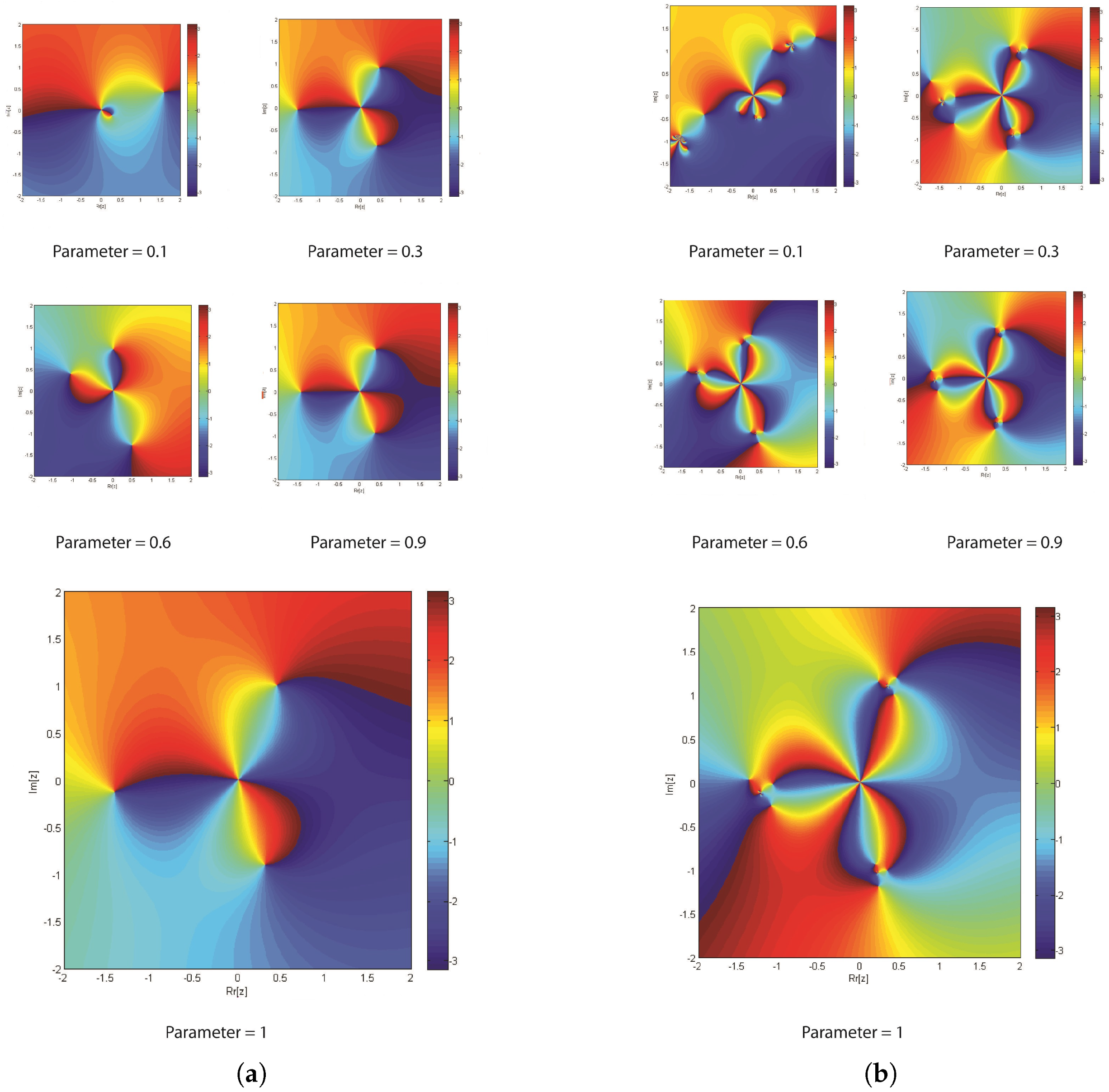
In order to solve a polynomial equation using the inverse fractional simultaneous iterative method, it is often useful to examine the basins of attraction [68,69] of the equation’s roots. The inverse fractional simultaneous scheme will eventually converge to a particular polynomial root in the basins of attraction of the complex plane. To identify the basins of attraction for (1) using the inverse fractional simultaneous scheme, we use a grid of ${[800\times 800]}^2$ points in the domain $\left[-2,2\right]\times \left[-2,2\right]$ of the complex plane encompassing the region of interest. We show the basins of attraction for the polynomial equation

$$f_1\left(\upsilon \right)={\upsilon }^4+{\upsilon }^2+\upsilon -1,$$

for which the Caputo-type derivative is given as

$$\left[{}_C{⅁}_{{\varsigma }_1}^{\varsigma }\right]f_1\left(\upsilon \right)=\frac{\lceil \left(5\right)}{\lceil (5-\varsigma )}{\upsilon }^{4-\varsigma }+\frac{\lceil \left(3\right)}{\lceil (3-\varsigma )}{\upsilon }^{2-\varsigma }+\frac{\lceil \left(2\right)}{\lceil (2-\varsigma )}{\upsilon }^{1-\varsigma }+\frac{1}{\lceil (1-\varsigma )}{\upsilon }^{-\varsigma }.$$

We use an inverse numerical scheme to solve the polynomial equation, starting from that grid of points. We observe the behavior of the iterations for each point until it converges to one of the roots of the polynomial equation within a tolerance of ${10}^{-3}$ on the error or until a predetermined number of iteration steps have been performed. Each grid point is colored or shaded based on the polynomial root to which it converges. This will provide a visual representation of the basins of attraction of (1). It is important to note that the inverse simultaneous scheme converges to a root for initial points that are far from any of the roots or are in a region with complex dynamics. This demonstrates the global convergence behavior of the numerical scheme.

In

Table 2. Results of percentage convergence and divergence in dynamical analysis.

Method	FINS${}_{{\mathit{\varsigma }}_1}$	FINS${}_{{\mathit{\varsigma }}_2}$	FINS${}_{{\mathit{\varsigma }}_3}$	FINS${}_{{\mathit{\varsigma }}_4}$	FINS${}_{{\mathit{\varsigma }}_5}$
E-Time	0.312512	0.125112	0.21453	0.125434	0.0125434
It-N	11	7	6	4	3
TT-Points	64,000.00	64,000.00	64,000.00	64,000.00	64,000.00
C-Points	50,154.00	51,425.12	52,145.00	52,894.56	63,870.31
D-Points	13,846	12,574.88	11,855	11,105.44	129.69
Per-Convergence	78.36%	80.35%	81.47%	82.64%	99.79%
Per-Divergence	21.63%	19.64%	18.52%	17.35%	0.001%

and

Table 3. Results of percentage convergence and divergence in dynamical analysis.

Method	FINS${}_{{\mathit{\varsigma }}_{1\ast }}$	FINS${}_{{\mathit{\varsigma }}_{2\ast }}$	FINS${}_{{\mathit{\varsigma }}_{3\ast }}$	FINS${}_{{\mathit{\varsigma }}_{4\ast }}$	FINS${}_{{\mathit{\varsigma }}_{5\ast }}$
E-Time	0.21451	0.14521	0.01241	0.01542	0.00124
It-N	9	7	4	3	2
TT-Points	64,000.00	64,000.00	64,000.00	64,000.00	64,000.00
C-Points	57,250.36	59,463.89	60,061.45	63,142.28	63,998.56
D-Points	6749.640	4536.110	3938.550	857.7200	8.440000
Per-Convergence	89.45%	92.91%	93.84%	98.65%	99.990%
Per-Divergence	10.54%	7.100%	6.100%	1.300%	0.0001%

, E-Time denotes the elapsed time in seconds, It-N indicates the number of iterations, TT-Points represents the total number of grid points, C-Points denotes the convergent points, D-Points refers to the number of divergent points, and Per-Convergence and Per-Divergence are the percentage convergence and divergence of the numerical scheme used to generate the basins of attractions for various functional parameters. Figure 3a,b and Table 2 and Table 3 both clearly demonstrate that the rate of convergence increases from 0.1 to 1.0, showing the global convergence of FINS${}_{{\varsigma }_{1\ast }}$ and FINS${}_{\varsigma }$, respectively.

7. Analysis of Numerical Results

In this section, we illustrate a few numerical experiments to compare the performance of our proposed simultaneous methods, FINS${}_{\varsigma }-$FINS${}_{{\varsigma }_1}$ and FINS${}_{{\varsigma }_{1\ast }}-$FINS${}_{{\varsigma }_{1\ast }}$ of order ten, to that of the ANN in some real-world applications. The calculations were carried out in quadruple-precision (128-bit) floating-point arithmetic using Maple 18. The algorithm was terminated based on the stopping criterion: $\mathrm{e}{}_i^{\left(\sigma \right)}=\left|\left({\upsilon }_i^{\left(\sigma +1\right)}-{\upsilon }_i^{\left(\sigma \right)}\right)\right|<\in ={10}^{-30}$ where $e_i^{\left(\sigma \right)}$ represents the absolute error. The stopping criteria for both the fractional inverse numerical simultaneous method and the ANN training were 5000 iterations and $e={10}^{-18}$. The elapsed times were obtained using a laptop equipped with a third-generation Intel Core i3 CPU and 4 GB of RAM. In our experiments, we compare the results of the newly developed fractional numerical schemes FINS${}_{\varsigma 1}$–FINS${}_{\varsigma 5}$ and FINS${}_{\varsigma 1\ast }$–FINS${}_{\varsigma 5\ast }$ to the Weierstrass method (WDKM), defined as

$$u_i^{\left(\sigma \right)}={\upsilon }_i^{\left(\sigma \right)}-\frac{f\left({\upsilon }_i^{\left(\sigma \right)}\right)}{\underset{\stackrel{j=1}{j\ne i}}{\stackrel{n}{\Pi }}({\upsilon }_i^{\left(\sigma \right)}-{\upsilon }_j^{\left(\sigma \right)})},$$

the convergent method by Zhang et al. (ZPHM), defined as

$$u_i^{\left(\sigma \right)}={\upsilon }_i^{\left(\sigma \right)}-\frac{2w_i\left({\upsilon }_i^{\left(\sigma \right)}\right)}{1+{\displaystyle \sum _{\underset{j=1}{j\ne i}}^n}\frac{w_j\left({\upsilon }_i^{\left(\sigma \right)}\right)}{{\upsilon }_i^{\left(\sigma \right)}-{\upsilon }_j^{\left(\sigma \right)}}+\sqrt{\begin{array}{c}{\left(1+{\displaystyle \sum _{\underset{j=1}{j\ne i}}^n}\frac{w_j\left({\upsilon }_i^{\left(\sigma \right)}\right)}{{\upsilon }_i^{\left(\sigma \right)}-{\upsilon }_j^{\left(\sigma \right)}}\right)}^2+4w_i\left({\upsilon }_i^{\left(\sigma \right)}\right)\\ \sum _{\underset{j=1}{j\ne i}}^n\frac{w_j\left({\upsilon }_i^{\left(\sigma \right)}\right)}{\left({\upsilon }_i^{\left(\sigma \right)}-{\upsilon }_j^{\left(\sigma \right)}\right)\left({\upsilon }_i^{\left(\sigma \right)}-w_i\left({\upsilon }_i^{\left(\sigma \right)}\right)-{\upsilon }_j^{\left(\sigma \right)}\right)}\end{array}}},$$

(41)

and the Petkovic method (MPM), defined as

$$u_i^{\left(\sigma \right)}={\upsilon }_i^{\left(\sigma \right)}-\frac{1}{\frac{1}{N_i\left({\upsilon }_i^{\left(\sigma \right)}\right)}-{\displaystyle \sum _{\stackrel{j=1}{j\ne i}}^n}\frac{1}{({\upsilon }_i^{\left(\sigma \right)}-Z_j^{\left(\sigma \right)}))}},$$

(42)

where $Z_j^{\left(\sigma \right)}={\upsilon }_j^{\left(\sigma \right)}-\frac{f\left(y_j^{\left(\sigma \right)}\right)-f\left({\upsilon }_j^{\left(\sigma \right)}\right)}{2f\left(y_j^{\left(\sigma \right)}\right)-f\left({\upsilon }_j^{\left(\sigma \right)}\right)}\frac{f\left({\upsilon }_j^{\left(\sigma \right)}\right)}{f^{\prime }\left({\upsilon }_j^{\left(\sigma \right)}\right)}$ and $y_j^{\left(\sigma \right)}={\upsilon }_j^{\left(\sigma \right)}-\frac{f\left({\upsilon }_j^{\left(\sigma \right)}\right)}{f^{\prime }\left({\upsilon }_j^{\left(\sigma \right)}\right)}.$ We generate random starting guess values using Algorithms 1 and 2, as shown in

Table A1. The ANN is trained using the head of the input data set to locate the real and imaginary roots of polynomial equations in engineering application 1.

${\mathit{a}}_0$	${\mathit{a}}_1$	${\mathit{a}}_2$	${\mathit{a}}_3$	${\mathit{a}}_4$
1.000	−0.160	0.643	0.967	0.085
0.757	0.743	0.392	0.655	0.171
0.121	−0.145	0.874	0.475	0.876
⋮	⋮	⋮	⋮	⋮

,

Table A2. The ANN is trained using the head of the input data set to locate the real and imaginary roots of polynomial equations in engineering application 2.

${\mathit{a}}_0$	${\mathit{a}}_1$	${\mathit{a}}_2$	${\mathit{a}}_3$	${\mathit{a}}_4$	${\mathit{a}}_5$	${\mathit{a}}_6$	${\mathit{a}}_7$	${\mathit{a}}_8$
1.000	−0.760	0.643	0.967	0.881	0.760	0.643	0.967	0.085
0.757	−0.153	0.392	0.615	0.171	0.743	0.392	0.855	0.071
0.934	−0.905	0.874	0.473	0.076	0.145	0.874	0.775	0.076
⋮	⋮	⋮	⋮	⋮	⋮	⋮	⋮	⋮

,

Table A3. The ANN is trained using the head of the input data set to locate the real and imaginary roots of polynomial equations in engineering application 3.

${\mathit{a}}_0$	${\mathit{a}}_1$	${\mathit{a}}_2$	${\mathit{a}}_3$	${\mathit{a}}_4$	${\mathit{a}}_5$	${\mathit{a}}_6$	${\mathit{a}}_7$	${\mathit{a}}_8$	${\mathit{a}}_9$	${\mathit{a}}_{10}$
$0.21\times {10}^{-4}$	$4.87\times {10}^{-4}$	$5.66\times {10}^{-3}$	$9.5\times {10}^{-5}$	$7.2\times {10}^{-8}$	$0.9\times {10}^{-7}$	$0.3\times {10}^{-4}$	$8.2\times {10}^{-3}$	$8.2\times {10}^{-8}$	1.78914	2.5733
$3.01\times {10}^{-4}$	$0.98\times {10}^{-3}$	$0.56\times {10}^{-3}$	$8.3\times {10}^{-7}$	$4.2\times {10}^{-4}$	$0.8\times {10}^{-8}$	$3.2\times {10}^{-4}$	$2.2\times {10}^{-8}$	$6.2\times {10}^{-8}$	2.01241	1.9342
$0.14\times {10}^{-3}$	$4.14\times {10}^{-5}$	$4.1\times {10}^{-4}$	$2.34\times {10}^{-8}$	$1.1\times {10}^{-3}$	$5.1\times {10}^{-7}$	$7.1\times {10}^{-6}$	$7.1\times {10}^{-4}$	$5.1\times {10}^{-7}$	1.21540	1.5435
⋮	⋮	⋮	⋮	⋮	⋮	⋮	⋮	⋮	⋮	⋮

,

Table A4. The ANN is trained using the head of the input data set to locate the real and imaginary roots of polynomial equations in engineering application 4.

${\mathit{a}}_0$	${\mathit{a}}_1$	${\mathit{a}}_2$	${\mathit{a}}_3$	${\mathit{a}}_4$
0.001	−0.760	0.043	0.967	0.085
0.857	0.743	0.392	0.159	0.171
0.021	−0.145	0.874	0.475	0.876
⋮	⋮	⋮	⋮	⋮

,

Table A5. The ANN is trained using the head of the output data set to locate the real and imaginary roots of polynomial equations in engineering application 1.

${\mathit{a}}_0$		${\mathit{a}}_1$		${\mathit{a}}_2$		${\mathit{a}}_3$		${\mathit{a}}_4$
Re($a_0$)	Im($a_0$)	Re($a_1$)	Im($a_1$)	Re($a_2$)	Im($a_2$)	Re($a_3$)	Im($a_3$)	Re($a_4$)	Im($a_4$)
0.124	0.98	0.56	8.31	4.25	0.124	0.98	0.56	8.31	4.25
0.145	4.14	4.11	2.31	1.14	0.145	4.14	4.11	2.31	1.14
⋮	⋮	⋮	⋮	⋮	⋮	⋮	⋮	⋮	⋮

, and

Table A6. The ANN is trained using the head of the output data set to locate the real and imaginary roots of polynomial equations in engineering application 4.

${\mathit{a}}_0$		${\mathit{a}}_1$		${\mathit{a}}_2$		${\mathit{a}}_3$		${\mathit{a}}_4$
Re($a_0$)	Im($a_0$)	Re($a_1$)	Im($a_1$)	Re($a_2$)	Im($a_2$)	Re($a_3$)	Im($a_3$)	Re($a_4$)	Im($a_4$)
0.124	0.98	0.56	8.31	4.25	0.124	0.98	0.56	8.31	4.25
0.145	4.14	4.11	2.31	1.14	0.145	4.14	4.11	2.31	1.14
⋮	⋮	⋮	⋮	⋮	⋮	⋮	⋮	⋮	⋮

. The parameter values utilized in the numerical results are reported below.

The ANN parameter values utilized in examples 1–4.

$\varsigma =[0.1,0.3,0.7,0.8,1.0]$

Epochs: $[77,57,38,43]$

MSE: $[3.0611\times {10}^{-7},6.1691\times {10}^{-6},1.1914\times {10}^{-9},6.0489\times {10}^{-9}]$

Gradient: $[9.931\times {10}^{-6},9.8016\times {10}^{-6},9.9911\times {10}^{-6},3.0416\times {10}^{-4}]$

Mu: $[0.1\times {10}^{-4},1.0\times {10}^{-5},1.1\times {10}^{-4},1.0\times {10}^{-6}]$

Real-World Applications

In this section, we apply our new inverse methods FINS${}_{{\varsigma }_1}-$FINS${}_{{\varsigma }_5}$ and FINS${}_{{\varsigma }_{1\ast }}-$FINS${}_{{\varsigma }_{1\ast }}$ to solve some real-world applications.

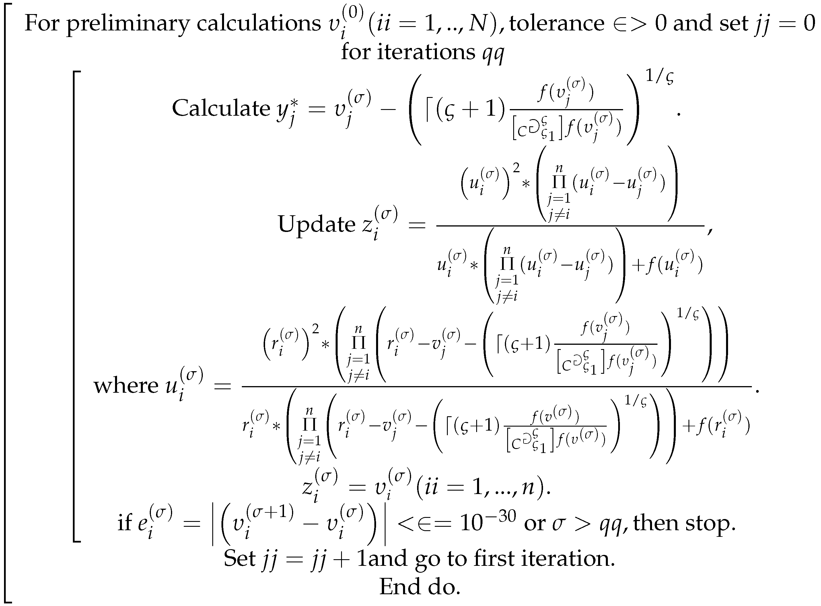
Algorithm 1 Inverse fractional numerical scheme: FINS${}_{{\varsigma }_{\mathbf{1}\ast }}$

Algorithm 2 Finding the random co-efficient of the polynomial

Example 1

(Quarter-car suspension model).

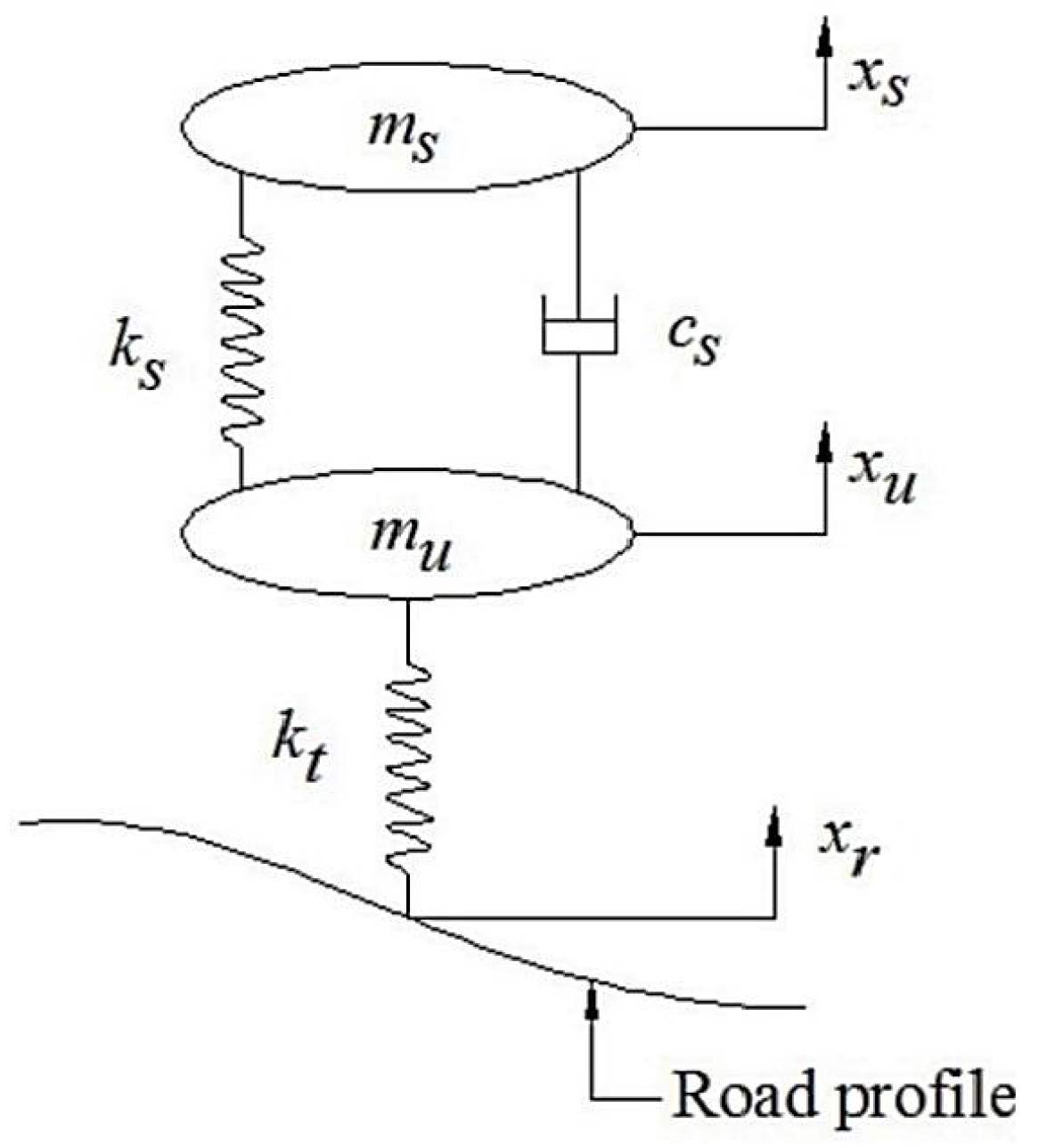
The shock absorber, or damper, is a component of the suspension system that is used to control the transient behavior of the vehicle mass and the suspension mass (see Pulvirenti [70] and Konieczny [71]). Because of its nonlinear behavior, it is one of the most complicated suspension system components. The damping force of the damper is characterized by an asymmetric nonlinear hysteresis loop (Liu [72]). In this example, the vehicle’s characteristics are simulated using a quarter-car model with two degrees of freedom, and the damper effect is investigated using linear and nonlinear damping characteristics. Simpler models, such as linear and independently linear ones, fall short of explaining the damper’s actions. The mass motion equations are as follows:

$$\left\{\begin{array}{c}{m}_s{\upsilon }_s^{\prime \prime }+k_s({\upsilon }_s-{\upsilon }_u)+F=0,\\ m_u{\upsilon }_u^{\prime \prime }-k_s({\upsilon }_s-{\upsilon }_u)-k_{\sigma }({\upsilon }_r-{\upsilon }_u)-F=0,\end{array}\right.$$

(43)

where $k_s$ and $k_{\sigma }$ are the spring stiffness and suspension coefficients in the tire stiffness system; $m_s$ and $m_u$ are the over- and under-sprung masses; and ${\upsilon }_s$ and ${\upsilon }_u$ are the displacements of the over- and under-masses.

The coefficient of damping force F in (43) is approximated by the polynomial [73]:

$$f_2\left(\upsilon \right)=-77.14\ast {\upsilon }^4+23.14\ast {\upsilon }^3+342.7\ast {\upsilon }^2+956.7x+124.5,$$

(44)

measuring the displacement, velocity, and acceleration of a mass over time. Figure 4 illustrates how the model can be used to develop and optimize vehicle systems for a range of driving situations, including comfort during travel, interacting with others, and stability.

The Caputo-type derivative of (44) is given as:

$$\begin{array}{ccc}\hfill \left[{}_C{⅁}_{{\varsigma }_1}^{\varsigma }\right]f_2\left(\upsilon \right)& =& -77.14\ast \frac{\lceil \left(5\right)}{\lceil (5-\varsigma )}{\upsilon }^{4-\varsigma }+23.14\ast \frac{\lceil \left(4\right)}{\lceil (4-\varsigma )}{\upsilon }^{3-\varsigma }+342.7\ast \frac{\lceil \left(3\right)}{\lceil (3-\varsigma )}{\upsilon }^{2-\varsigma }\hfill \\ & & +956.7\frac{\lceil \left(2\right)}{\lceil (2-\varsigma )}{\upsilon }^{1-\varsigma }+124.5\frac{1}{\lceil (1-\varsigma )}{\upsilon }^{-\varsigma }.\hfill \end{array}$$

The exact roots of Equation (44) are

$$\begin{array}{ccc}\hfill {\zeta }_1& =& 3.090556803,{\zeta }_2=-1.326919946+1.434668028\ast i,{\zeta }_3=-0.1367428388,\hfill \\ \hfill {\zeta }_4& =& -1.32060919946-1.43046068028\ast i.\hfill \end{array}$$

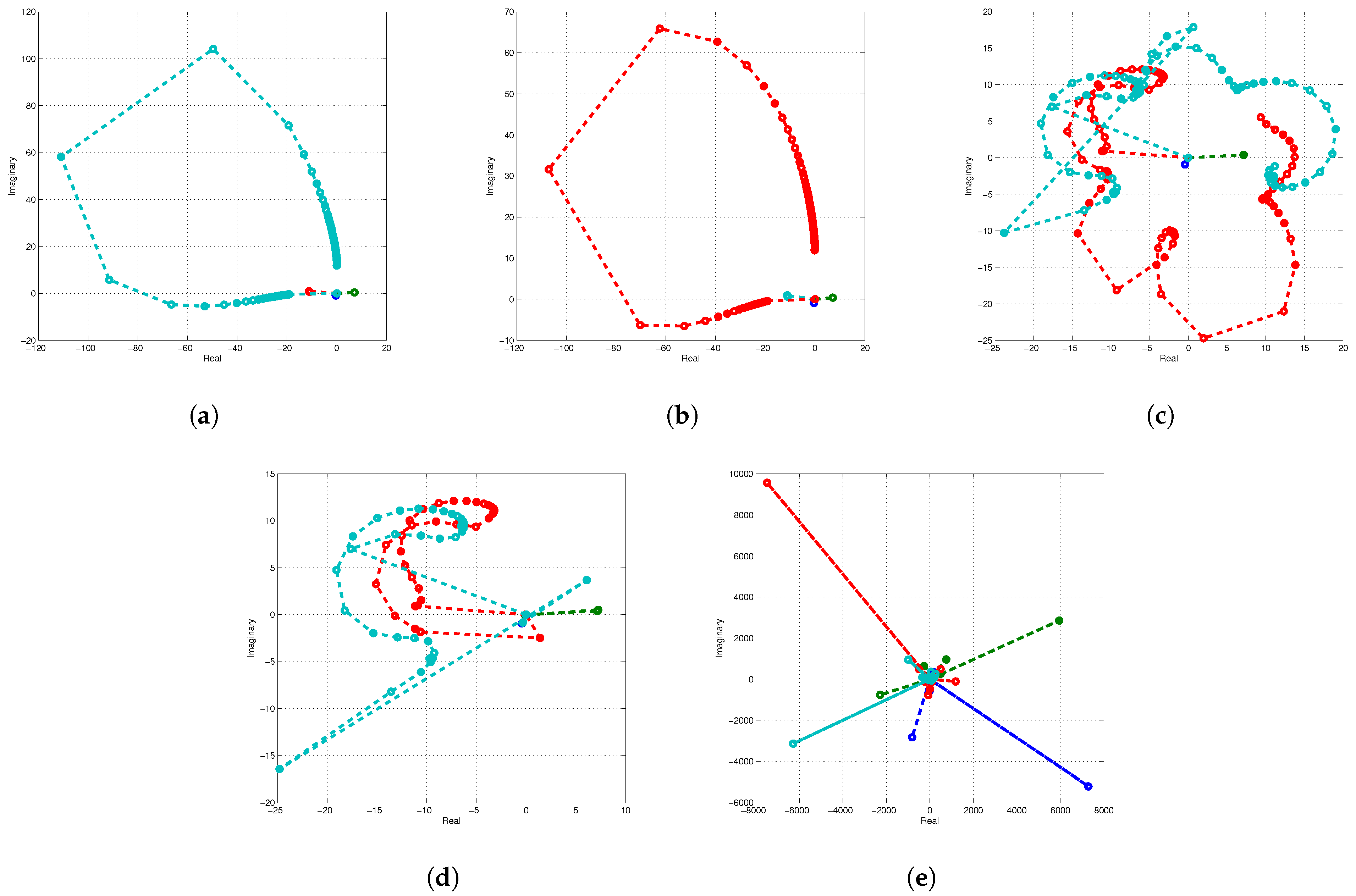
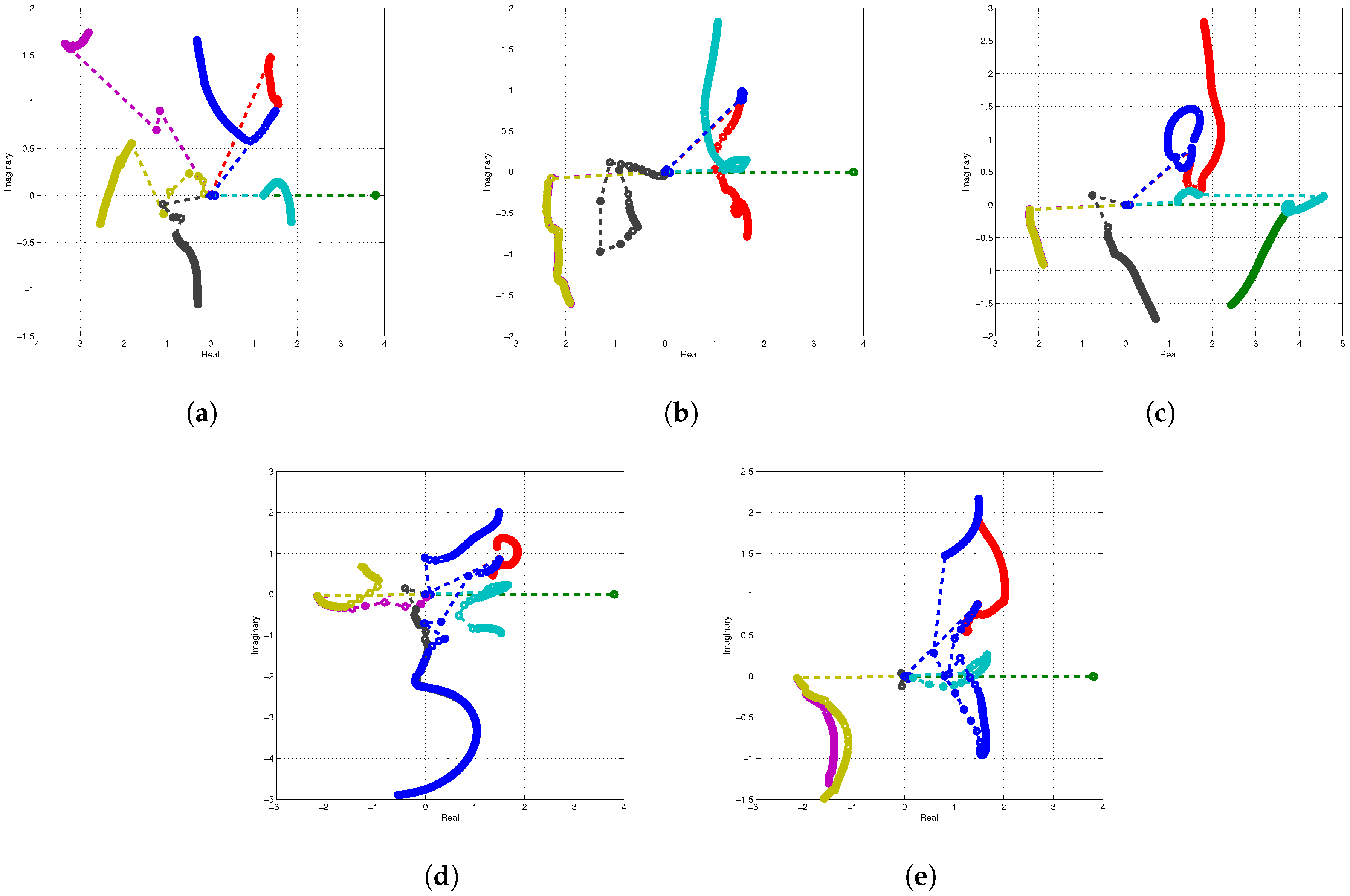
Next, the convergence rate and computational order of the numerical schemes FINS${}_{{\varsigma }_{1\ast }}$–FINS${}_{{\varsigma }_{5\ast }}$ are defined. In order to quantify the global convergence rate of the inverse parallel fractional scheme, a random initial guess value $v=$ [0.213, 0.124, 1.02, 1425] is generated using the built-in MATLAB rand() function. With a random initial estimate, FINS${}_{{\varsigma }_{1\ast }}$ converges to the exact roots after 9, 8, 7, and 7 iterations and requires, respectively, 0.04564, 0.07144, 0.07514, 0.01247, and 0.045451 s to converge for different fractional parameters, i.e., 0.1, 0.3, 0.5, 0.8, and 1.0. The results in

Table 4. Approximation of all polynomial equation roots using FINS${}_{{\varsigma }_{1\ast }}$–FINS${}_{{\varsigma }_{5\ast }}$ methods.

Method	Iter	${\mathit{e}}_1^{\left(\mathit{\sigma }\right)}$	${\mathit{e}}_2^{\left(\mathit{\sigma }\right)}$	${\mathit{e}}_3^{\left(\mathit{\sigma }\right)}$	${\mathit{e}}_4^{\left(\mathit{\sigma }\right)}$	${\mathit{\rho }}_{\mathit{\varsigma }\mathit{i}}^{(\mathit{\sigma }-1)}$	C-Time
$\mathbf{v}$ = [0.213,0.124,1.02,1425]: Random initial approximation
FINS${}_{{\varsigma }_{1\ast }}$	9	$0.12\times {10}^{-3}$	$9.72\times {10}^{-3}$	$6.62\times {10}^{-10}$	$0.29\times {10}^{-8}$	1.09915	0.04564
FINS${}_{{\varsigma }_{2\ast }}$	8	$1.24\times {10}^{-6}$	$6.78\times {10}^{-7}$	$7.27\times {10}^{-7}$	$0.46\times {10}^{-8}$	1.24512	0.07144
FINS${}_{{\varsigma }_{3\ast }}$	8	$4.32\times {10}^{-9}$	$9.25\times {10}^{-7}$	$9.25\times {10}^{-3}$	$0.76\times {10}^{-10}$	1.46514	0.07514
FINS${}_{{\varsigma }_{4\ast }}$	7	$6.17\times {10}^{-3}$	$5.17\times {10}^{-5}$	$6.15\times {10}^{-4}$	$0.61\times {10}^{-11}$	1.78945	0.01247
FINS${}_{{\varsigma }_{5\ast }}$	7	$0.91\times {10}^{-2}$	$1.71\times {10}^{-8}$	$0.16\times {10}^{-5}$	$3.54\times {10}^{-9}$	2.01241	0.04545

clearly indicate that as the value of $\varsigma$ grows from 0.1 to 1.0, the rate of convergence of FINS${}_{{\varsigma }_{1\ast }}$ increases. Unlike ANNs, our newly developed algorithm converges to the exact roots for a range of random initial guesses, confirming a global convergence behavior.

When the initial approximation is close to the exact roots, the rate of convergence increases significantly, as illustrated in

Table 5. Simultaneous approximation of all polynomial equation roots.

Method	FINS${}_{{\mathit{\varsigma }}_1}$	FINS${}_{{\mathit{\varsigma }}_2}$	FINS${}_{{\mathit{\varsigma }}_3}$	FINS${}_{{\mathit{\varsigma }}_4}$	FINS${}_{{\mathit{\varsigma }}_5}$
Error it	4	4	16	16	16
CPU	0.0756	0.0566	0.0345	0.0213	0.01761
$e_1^{\left(\sigma \right)}$	$0.26\times {10}^{-5}$	$0.75\times {10}^{-6}$	$0.26\times {10}^{-9}$	$0.2\times {10}^{-36}$	$5.6\times {10}^{-31}$
$e_2^{\left(\sigma \right)}$	$7.1\times {10}^{-6}$	$0.56\times {10}^{-7}$	$5.17\times {10}^{-7}$	$0.51\times {10}^{-27}$	$4.5\times {10}^{-38}$
$e_3^{\left(\sigma \right)}$	$8.18\times {10}^{-10}$	$1.16\times {10}^{-26}$	$8.18\times {10}^{-37}$	$4.1\times {10}^{-82}$	$4.1\times {10}^{-98}$
$e_4^{\left(\sigma \right)}$	$3.17\times {10}^{-20}$	$3.18\times {10}^{-5}$	$3.71\times {10}^{-20}$	$3.51\times {10}^{-29}$	$3.4\times {10}^{-35}$
${\rho }_{\varsigma i}^{(\sigma -1)}$	2.01412	2.235423	2.453641	2.87187	3.14154

and

Table 6. Simultaneous approximation of all polynomial equation roots.

Method	FINS${}_{{\mathit{\varsigma }}_{1\ast }}$	FINS${}_{{\mathit{\varsigma }}_{2\ast }}$	FINS${}_{{\mathit{\varsigma }}_{3\ast }}$	FINS${}_{{\mathit{\varsigma }}_{4\ast }}$	FINS${}_{{\mathit{\varsigma }}_{5\ast }}$
Error it	5	4	4	3	2
CPU	0.054185	0.03612	0.04412	0.06774	0.065785
$e_1^{\left(\sigma \right)}$	$0.2\times {10}^{-7}$	$0.29\times {10}^{-15}$	$0.2\times {10}^{-31}$	$0.2\times {10}^{-39}$	$0.2\times {10}^{-65}$
$e_2^{\left(\sigma \right)}$	$0.14\times {10}^{-8}$	$8.91\times {10}^{-20}$	$0.1\times {10}^{-36}$	$0.1\times {10}^{-45}$	$0.1\times {10}^{-90}$
$e_3^{\left(\sigma \right)}$	$1.14\times {10}^{-15}$	$1.19\times {10}^{-29}$	$1.1\times {10}^{-38}$	$1.1\times {10}^{-52}$	$1.1\times {10}^{-86}$
$e_4^{\left(\sigma \right)}$	$3.91\times {10}^{-8}$	$3.18\times {10}^{-12}$	$3.1\times {10}^{-40}$	$3.1\times {10}^{-32}$	$3.1\times {10}^{-76}$
${\rho }_{\varsigma i}^{(\sigma -1)}$	2.09812	2.09231	2.671	3.0341	3.34423

.

The following initial estimate values increase the convergence rates:

$$\stackrel{\left(0\right)}{{\upsilon }_1}=2.0,\stackrel{\left(0\right)}{{\upsilon }_2}=-1+5i,{\stackrel{\left(0\right)}{\upsilon }}_3=-0.5,{\stackrel{\left(0\right)}{\upsilon }}_4=-1-5i.$$

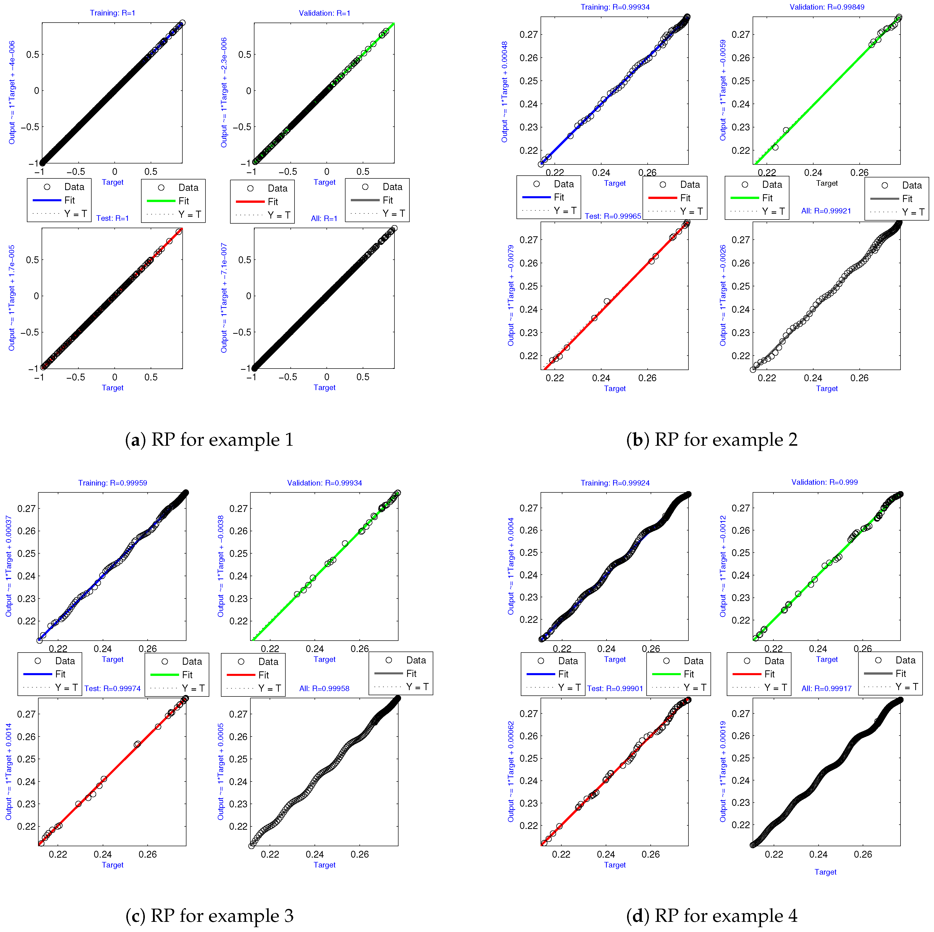
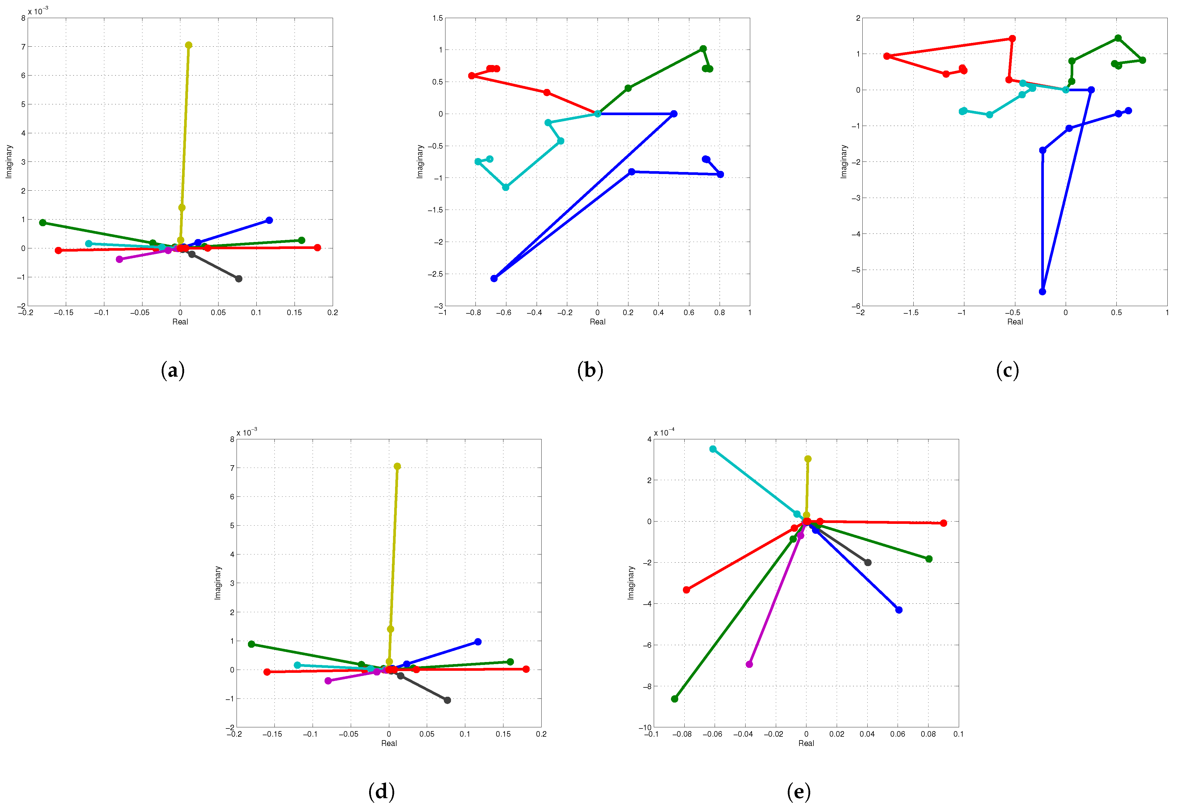
The outcomes of the ANN-based inverse simultaneous schemes (ANNFN${}_{{\varsigma }_{1\ast }}$–ANNFN${}_{{\varsigma }_{5\ast }}$) are shown in

Table 7. Numerical results using an artificial neural network on application 1.

Method	ANNFN${}_{{\mathit{\varsigma }}_{1\ast }}$	ANNFN${}_{{\mathit{\varsigma }}_{2\ast }}$	ANNFN${}_{{\mathit{\varsigma }}_{3\ast }}$	ANNFN${}_{{\mathit{\varsigma }}_{4\ast }}$	ANNFN${}_{{\mathit{\varsigma }}_{5\ast }}$
Error it	15	10	11	12	9
Ex-Time	0.016	0.054	0.067	0.065	0.071
$e_1^{\left(\sigma \right)}$	$6.62\times {10}^{-3}$	$8.62\times {10}^{-6}$	$9.52\times {10}^{-5}$	$8.82\times {10}^{-8}$	$3.3\times {10}^{-20}$
$e_2^{\left(\sigma \right)}$	$4.51\times {10}^{-4}$	$9.15\times {10}^{-7}$	$9.91\times {10}^{-4}$	$0.17\times {10}^{-9}$	$6.1\times {10}^{-26}$
$e_3^{\left(\sigma \right)}$	$7.16\times {10}^{-4}$	$7.15\times {10}^{-8}$	$1.41\times {10}^{-8}$	$1.91\times {10}^{-8}$	$1.1\times {10}^{-22}$
$e_4^{\left(\sigma \right)}$	$3.15\times {10}^{-2}$	$3.13\times {10}^{-8}$	$3.31\times {10}^{-9}$	$3.61\times {10}^{-7}$	$3.7\times {10}^{-23}$
MSE	$6.15\times {10}^{-7}$	$9.13\times {10}^{-8}$	$3.31\times {10}^{-3}$	$0.61\times {10}^{-4}$	$4.71\times {10}^{-5}$
Per-E	99.12%	98.87%	97.74%	98.31%	99.98%

. The real coefficients of the nonlinear equations utilized in engineering application 1 were fed into the ANNs, and the output was the exact roots of the relevant nonlinear equations, as shown in Figure 1. The head of the data set utilized in the ANNs is shown in Table A1 and Table A5, which provides the approximate root of the nonlinear equation used in engineering application 1 as an output. To generate the data sets, polynomial coefficients were produced at random in the interval [0, 1], and the exact roots were calculated using Matlab. According to Appendix A Table A1, the ANNs are currently unaware of which roots are real and which roots are complex; therefore, the ANNs were trained using $70\%$ of the samples from these data sets. The remaining $30\%$ was utilized to assess the ANNs’ generalization skills by computing a performance metric on the samples that were not used to train the ANNs. For a polynomial of degree 4, the ANN required 5 input data points, two hidden layers, and 10 output data points (the real and imaginary parts of the calculated root). In order to represent all the roots of engineering application 1, Figure 5a, Figure 6a, Figure 7a, Figure 8a, Figure 9a, display the error histogram (EPH), mean square error (MSE), regression plot (RP), transition statistics (TS), and fitness overlapping graphs of the target and outcomes of the LMA-ANN for each instance’s training, testing, and validation. Table 7 provides a summary of the performance of ANNFN${}_{{\varsigma }_{1\ast }}$–ANNFN${}_{{\varsigma }_{5\ast }}$ in terms of the mean square error (MSE), percentage effectiveness (Per-E), execution time in seconds (Ex-time), and iteration number (Error-it).

The numerical results of the simultaneous schemes with initial guess values that vary close to the exact roots are shown in

Table 8. A comparison of the simultaneous schemes’ numerical results utilizing initial guess values that are close to the exact roots.

Method	WDKM	FINS${}_{\mathit{\varsigma }}$	ZPHM	MPCM	ANNFN${}_{{\mathit{\varsigma }}_{5\ast }}$	FINS${}_{{\mathit{\varsigma }}_{5\ast }}$
CPU Time	0.06001	0.02404	0.03118	0.02515	0.01254	0.01104
$e_1^{\left(5\right)}$	$0.02\times {10}^{-3}$	$8.62\times {10}^{-24}$	$9.52\times {10}^{-35}$	$8.02\times {10}^{-45}$	$0.12\times {10}^{-27}$	$0.12\times {10}^{-65}$
$e_2^{\left(5\right)}$	$4.51\times {10}^{-4}$	$9.25\times {10}^{-35}$	$0.91\times {10}^{-24}$	$0.07\times {10}^{-59}$	$6.16\times {10}^{-28}$	$6.16\times {10}^{-63}$
$e_3^{\left(5\right)}$	$4.16\times {10}^{-4}$	$6.15\times {10}^{-14}$	$1.62\times {10}^{-38}$	$0.91\times {10}^{-8}$	$0.16\times {10}^{-37}$	$2.16\times {10}^{-64}$
$e_4^{\left(5\right)}$	$4.35\times {10}^{-2}$	$2.03\times {10}^{-21}$	$4.31\times {10}^{-33}$	$8.68\times {10}^{-43}$	$3.01\times {10}^{-34}$	$7.71\times {10}^{-55}$
Max-Error	$0.15\times {10}^{-8}$	$9.13\times {10}^{-26}$	$2.31\times {10}^{-36}$	$0.61\times {10}^{-55}$	$0.75\times {10}^{-25}$	0.00
${\rho }^{\left(4\right)}$	1.812125	3.01224	5.013212	5.212312	3.4000245	6.0125417

. In terms of the residual error, CPU time, and maximum error (Max-Error), our new methods exhibit better results compared to the existing methods after the same number of iterations.

The proposed root-finding method, represented in Figure 1, is based on the Levenberg–Marquardt technique of artificial neural networks. The “nftool” fitting tool, which is included in the ANN toolkit in MATLAB, is used to approximate roots of polynomials with randomly generated coefficients.

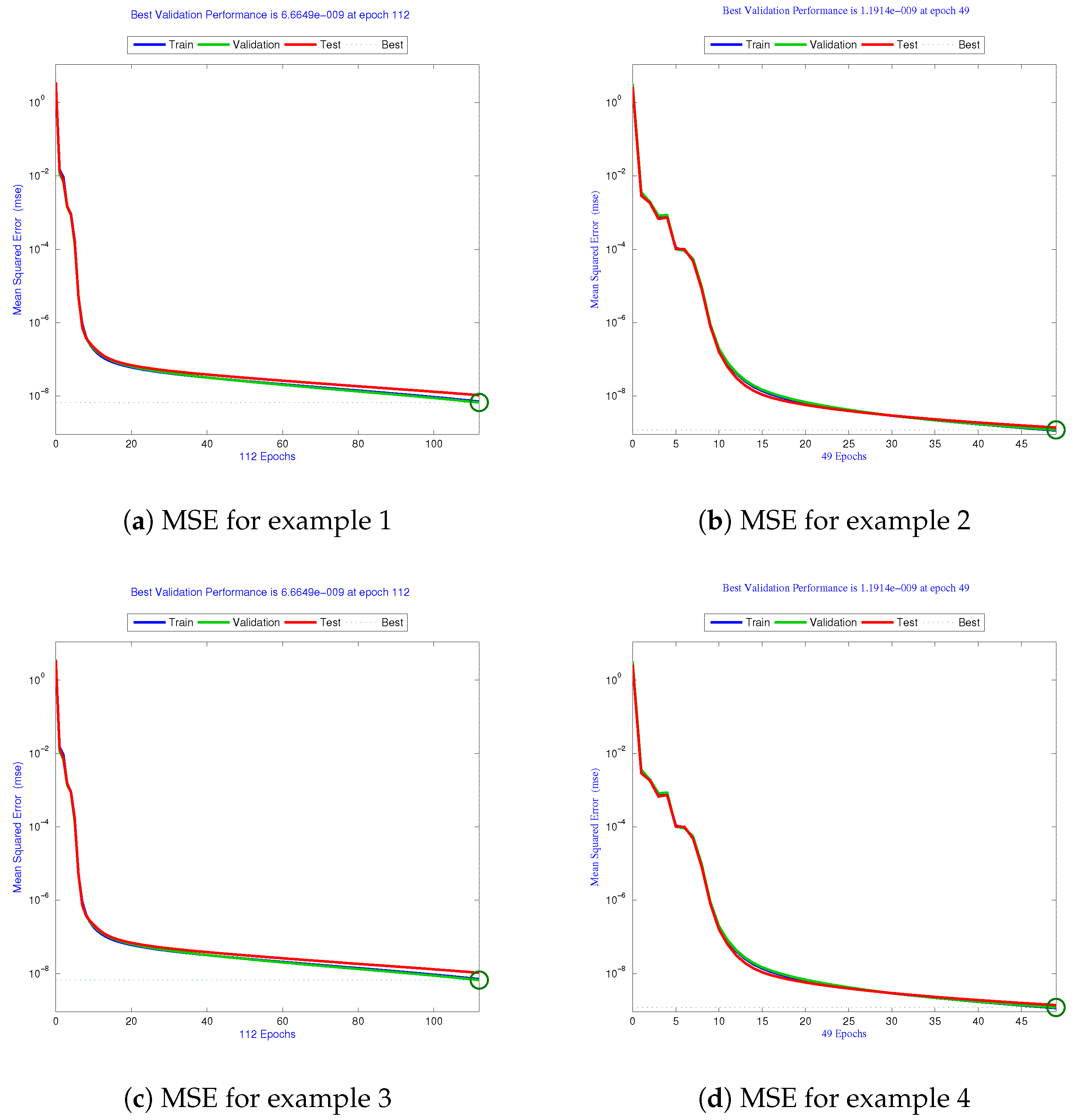
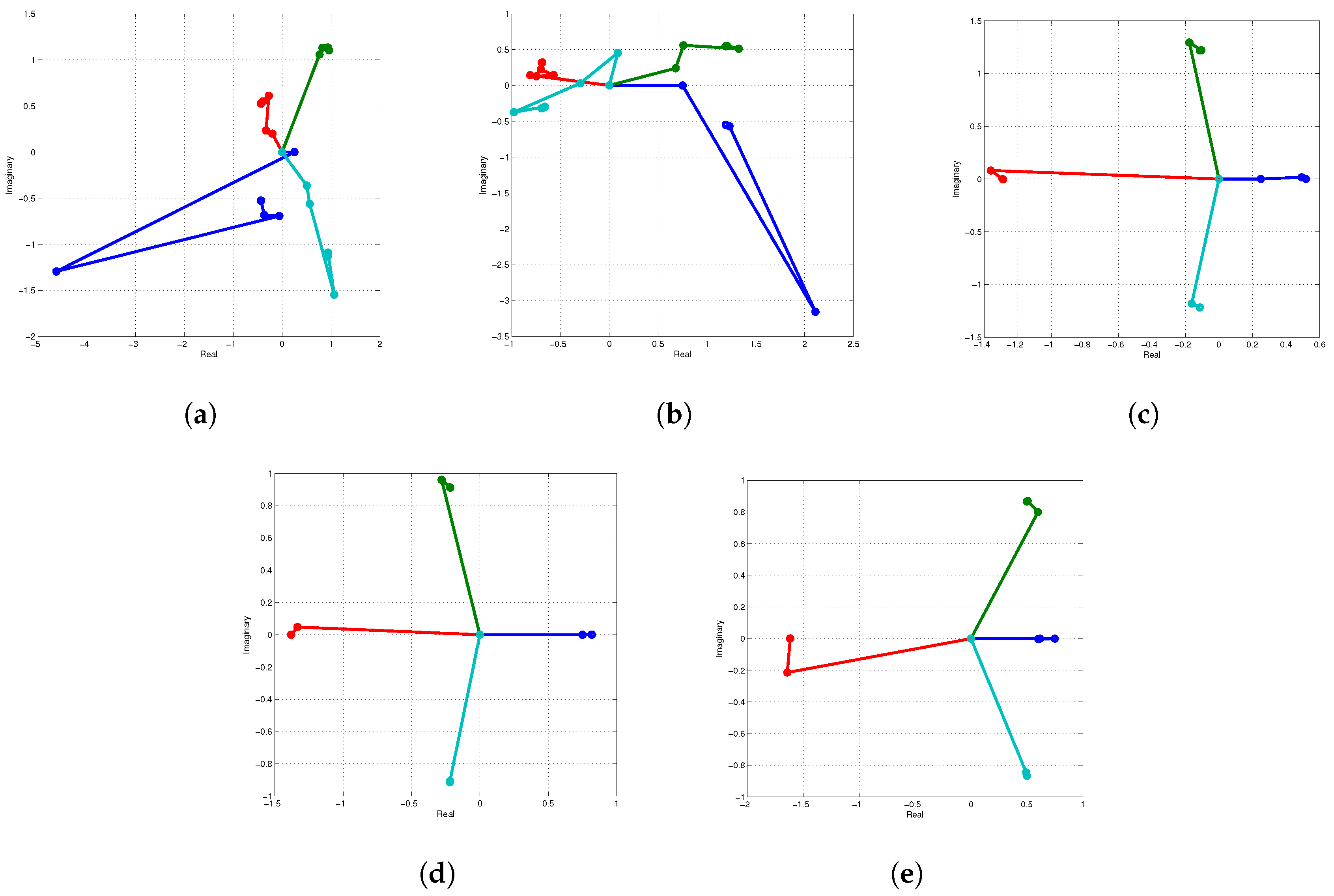
For training, testing, and validation, the input and output results of the LMA-ANNs’ fitness overlapping graphs are shown in Figure 5a. According to the histogram, the error is $6.2\times {10}^{-2}$, demonstrating the consistency of the suggested solver. For engineering application 1, the MSE of the LMA-ANNs when comparing the expected outcome to the target solution is $6.6649\times {10}^{-9}$ at epoch 112, as shown in Figure 6a. The expected and actual results of the LMA-ANNs are linearly related, as shown in Figure 7a. Figure 8a illustrates the efficiency, consistency, and reliability of the engineering application 1 simulation, where Mu is the adaptation parameter for the algorithm that trained the LMA-ANNs. The choice of Mu directly affects the error convergence and maintains its value in the range [0, 1]. For engineering application 1, the gradient value is $9.9314\times {10}^{-6}$ with a Mu parameter of $1.0\times {10}^{-4}$. Figure 8a shows how the results for the minimal Mu and gradient converge closer as the network becomes more efficient at training and testing. In turn, the fitness curve simulations and regression analysis simulations are displayed in Figure 9a. When R is near 1, the correlation is strong; however, it becomes unreliable when R approaches 0. A reduced MSE causes a decreased response time. Figure 10a–e depict the root trajectories for various initial estimate values.

Example 2

(Blood Rheology Model [75]).

Nanofluids are synthetic fluids made of nanoparticles dispersed in a liquid such as water or oil that are typically less than 100 nanometers in size. These nanoparticles can be used to improve the heat transfer capabilities or other properties of the base fluid. They are frequently chosen for their special thermal, electrical, or optical characteristics. Casson nanofluid, like other nanofluids, can be used in a variety of contexts, such as heat-transfer systems, the cooling of electronics, and even medical applications. The introduction of nanoparticles into a fluid can enhance its thermal conductivity and other characteristics, potentially leading to enhanced heat exchange or other intended results in specific applications. A basic fluid such as water or plasma will flow in a tube so that its center core travels as a plug with very little deflection and a velocity variance toward the tube wall according to the Casson fluid model. In our experiment, the plug flow of Casson fluids was described as:

$$G=1-\frac{16}{7}\sqrt{\upsilon }+\frac{4}{3}\upsilon -\frac{1}{21}{\upsilon }^4.$$

(45)

Using $G=0.40$ in Equation (45), we have:

$$f_3\left(\upsilon \right)=\frac{1}{441}{\upsilon }^8-\frac{8}{63}{\upsilon }^5-0.05714285714x^4+\frac{16}{9}{\upsilon }^2-3.624489796x+0.36.$$

(46)

The Caputo-type derivative of (46) is given as:

$$\begin{array}{ccc}\hfill \left[{}_C{⅁}_{{\varsigma }_1}^{\varsigma }\right]f_3\left(\upsilon \right)& =& \frac{1}{441}\frac{\lceil \left(9\right)}{\lceil (9-\varsigma )}{\upsilon }^{8-\varsigma }-\frac{8}{63}\frac{\lceil \left(6\right)}{\lceil (6-\varsigma )}{\upsilon }^{5-\varsigma }-0.05714285714\frac{\lceil \left(5\right)}{\lceil (5-\varsigma )}{\upsilon }^{4-\varsigma }\hfill \\ & & +\frac{16}{9}\frac{\lceil \left(3\right)}{\lceil (3-\varsigma )}{\upsilon }^{2-\varsigma }-3.624489796\frac{\lceil \left(2\right)}{\lceil (2-\varsigma )}{\upsilon }^{1-\varsigma }+0.36\frac{1}{\lceil (1-\upsilon )}{\upsilon }^{-\varsigma }.\hfill \end{array}$$

The exact roots of Equation (46) are:

$$\begin{array}{ccc}\hfill {\zeta }_1& =& 0.1046986515,{\zeta }_2=3.822389235,{\zeta }_3=1.553919850+0.9404149899i,\hfill \\ \hfill {\zeta }_4& =& -1.238769105+3.408523568i,{\zeta }_5=-2.278694688+1.987476450i,\hfill \\ \hfill {\zeta }_6& =& -2.278694688-1.987476450i,{\zeta }_7=-1.238769105-3.408523568,\hfill \\ \hfill {\zeta }_8& =& 1.553919850-0.9404149899.\hfill \end{array}$$

In order to quantify the global convergence rate of the inverse parallel fractional schemes FINS${}_{{\varsigma }_{1\ast }}$–FINS${}_{{\varsigma }_{5\ast }}$, a random initial guess value $v=$ [12.01, 14.56, 4.01, 45.5, 3.45, 78.9, 14.56, 47.89] is generated by the built-in MATLAB rand() function. With a random initial estimate, FINS${}_{{\varsigma }_{1\ast }}$ converges to the exact roots after 9, 8, 7, 6, and 5 iterations and requires, respectively, 0.04564, 0.07144, 0.07514, 0.01247, and 0.045451 s to converge for different fractional parameters, namely 0.1, 0.3, 0.5, 0.8, and 1.0. The results in

Table 9. Simultaneous approximation of all polynomial equation roots using FINS${\varsigma }_{1\ast }$–FINS${\varsigma }_{5\ast }$.

Method	${\mathit{e}}_1^{\left(\mathit{\sigma }\right)}$	${\mathit{e}}_2^{\left(\mathit{\sigma }\right)}$	${\mathit{e}}_3^{\left(\mathit{\sigma }\right)}$	${\mathit{e}}_4^{\left(\mathit{\sigma }\right)}$	${\mathit{e}}_5^{\left(\mathit{\sigma }\right)}$	${\mathit{e}}_6^{\left(\mathit{\sigma }\right)}$	${\mathit{e}}_7^{\left(\mathit{\sigma }\right)}$	${\mathit{e}}_8^{\left(\mathit{\sigma }\right)}$	${\mathit{\rho }}_{\mathit{\varsigma }\mathit{i}}^{(\mathit{\sigma }-1)}$	C-Time
$\mathbf{v}=$ [12.01, 14.56, 4.01, 45.5, 3.45, 78.9, 14.56, 47.89]: Random initial approximation
FINS${}_{{\varsigma }_{1\ast }}$	$7.2\times {10}^{-1}$	$2.7\times {10}^{-3}$	$8.7\times {10}^{-5}$	$0.2\times {10}^{-4}$	$8.2\times {10}^{-8}$	$0.3\times {10}^{-7}$	$2.2\times {10}^{-8}$	$9.2\times {10}^{-7}$	1.120	3.453
FINS${}_{{\varsigma }_{2\ast }}$	$4.8\times {10}^{-4}$	$5.6\times {10}^{-3}$	$9.5\times {10}^{-5}$	$7.2\times {10}^{-8}$	$0.9\times {10}^{-7}$	$0.3\times {10}^{-4}$	$8.2\times {10}^{-3}$	$8.2\times {10}^{-8}$	1.789	2.573
FINS${}_{{\varsigma }_{3\ast }}$	$0.9\times {10}^{-3}$	$0.5\times {10}^{-3}$	$8.3\times {10}^{-7}$	$4.2\times {10}^{-4}$	$0.8\times {10}^{-8}$	$3.2\times {10}^{-4}$	$2.2\times {10}^{-8}$	$6.2\times {10}^{-8}$	2.012	1.934
FINS${}_{{\varsigma }_{4\ast }}$	$4.1\times {10}^{-5}$	$4.1\times {10}^{-4}$	$2.3\times {10}^{-8}$	$1.1\times {10}^{-3}$	$5.1\times {10}^{-7}$	$7.1\times {10}^{-6}$	$7.1\times {10}^{-4}$	$5.1\times {10}^{-7}$	1.215	1.543
FINS${}_{{\varsigma }_{5\ast }}$	$8.1\times {10}^{-8}$	$8.1\times {10}^{-5}$	$1.2\times {10}^{-9}$	$1.1\times {10}^{-5}$	$1.1\times {10}^{-8}$	$1.1\times {10}^{-4}$	$1.1\times {10}^{-7}$	$1.1\times {10}^{-8}$	2.415	1.012

clearly indicate that as the value of $\varsigma$ grows from 0.1 to 1.0, the rate of convergence of FINS${}_{{\varsigma }_{1\ast }}$ increases. Unlike ANNs, our newly developed algorithm converges to the exact roots for a range of random initial guesses, confirming a global convergence behavior. Figure 11a–e depict the root trajectories for various initial estimate values. When the initial approximation is close to the exact roots, the rate of convergence increases significantly, as illustrated in

Table 10. Approximation of all polynomial equation roots.

Method	FINS${}_{{\mathit{\varsigma }}_1}$	FINS${}_{{\mathit{\varsigma }}_2}$	FINS${}_{{\mathit{\varsigma }}_3}$	FINS${}_{{\mathit{\varsigma }}_4}$	FINS${}_{{\mathit{\varsigma }}_5}$
Error it	10	8	8	7	6
CPU	0.0141	0.016	0.054	0.067	0.065
$e_1^{\left(\sigma \right)}$	$3.30\times {10}^{-6}$	$3.76\times {10}^{-16}$	$3.5\times {10}^{-26}$	$0.01\times {10}^{-36}$	$3.6\times {10}^{-37}$
$e_2^{\left(\sigma \right)}$	$1.62\times {10}^{-4}$	$1.26\times {10}^{-14}$	$4.23\times {10}^{-24}$	$1.72\times {10}^{-34}$	$6.2\times {10}^{-34}$
$e_3^{\left(\sigma \right)}$	$3.3\times {10}^{-3}$	$1.83\times {10}^{-13}$	$6.23\times {10}^{-23}$	$9.3\times {10}^{-33}$	$1.7\times {10}^{-39}$
$e_4^{\left(\sigma \right)}$	$1.04\times {10}^{-3}$	$9.68\times {10}^{-13}$	$5.44\times {10}^{-23}$	$7.84\times {10}^{-33}$	$1.6\times {10}^{-38}$
$e_5^{\left(\sigma \right)}$	$8.05\times {10}^{-3}$	$0.65\times {10}^{-10}$	$5.5\times {10}^{-10}$	$7.5\times {10}^{-22}$	$8.5\times {10}^{-35}$
$e_6^{\left(\sigma \right)}$	$2.05\times {10}^{-4}$	$0.66\times {10}^{-11}$	$5.75\times {10}^{-21}$	$0.76\times {10}^{-31}$	$6.6\times {10}^{-45}$
$e_7^{\left(\sigma \right)}$	$1.06\times {10}^{-3}$	$0.62\times {10}^{-12}$	$5.65\times {10}^{-23}$	$4.74\times {10}^{-33}$	$1.2\times {10}^{-56}$
$e_8^{\left(\sigma \right)}$	$4.04\times {10}^{-3}$	$4.6\times {10}^{-3}$	$7.45\times {10}^{-23}$	$7.43\times {10}^{-43}$	$4.3\times {10}^{-55}$
${\rho }_{\varsigma i}^{(\sigma -1)}$	2.1275	2.2374	2.5145	3.07445	3.5445

and

Table 11. Approximation of all polynomial equation roots.

Method	FINS${}_{{\mathit{\varsigma }}_{1\ast }}$	FINS${}_{{\mathit{\varsigma }}_{2\ast }}$	FINS${}_{{\mathit{\varsigma }}_{3\ast }}$	FINS${}_{{\mathit{\varsigma }}_{4\ast }}$	FINS${}_{{\mathit{\varsigma }}_{5\ast }}$
Error it	7	5	3	3	2
CPU	0.01678	0.05465	0.06745	0.06545	0.07154
$e_1^{\left(\sigma \right)}$	$0.36\times {10}^{-12}$	$3.40\times {10}^{-26}$	$6.33\times {10}^{-33}$	$0.26\times {10}^{-46}$	$1.55\times {10}^{-62}$
$e_2^{\left(\sigma \right)}$	$2.51\times {10}^{-16}$	$1.62\times {10}^{-24}$	$5.32\times {10}^{-31}$	$2.16\times {10}^{-43}$	$1.26\times {10}^{-61}$
$e_3^{\left(\sigma \right)}$	$3.62\times {10}^{-16}$	$1.83\times {10}^{-23}$	$9.23\times {10}^{-33}$	$1.56\times {10}^{-42}$	$4.15\times {10}^{-61}$
$e_4^{\left(\sigma \right)}$	$4.51\times {10}^{-16}$	$1.47\times {10}^{-23}$	$3.32\times {10}^{-37}$	$3.05\times {10}^{-53}$	$2.23\times {10}^{-62}$
$e_5^{\left(\sigma \right)}$	$6.54\times {10}^{-16}$	$0.75\times {10}^{-20}$	$1.25\times {10}^{-48}$	$2.65\times {10}^{-54}$	$3.14\times {10}^{-61}$
$e_6^{\left(\sigma \right)}$	$4.02\times {10}^{-17}$	$0.86\times {10}^{-21}$	$2.53\times {10}^{-48}$	$4.16\times {10}^{-55}$	$1.24\times {10}^{-61}$
$e_7^{\left(\sigma \right)}$	$3.03\times {10}^{-16}$	$1.28\times {10}^{-23}$	$3.13\times {10}^{-47}$	$1.31\times {10}^{-56}$	$4.55\times {10}^{-51}$
$e_8^{\left(\sigma \right)}$	$2.07\times {10}^{-16}$	$4.38\times {10}^{-23}$	$0.22\times {10}^{-31}$	$2.35\times {10}^{-43}$	$3.42\times {10}^{-52}$
${\rho }_{\varsigma i}^{(\sigma -1)}$	4.2374	3.9147	3.5112	3.142	2.151

.

The following initial estimate value results in an increase in the convergence rates:

$$\begin{array}{ccc}\hfill \stackrel{\left(0\right)}{{\upsilon }_1}& =& 0.1,\stackrel{\left(0\right)}{{\upsilon }_2}=3.8,{\stackrel{\left(0\right)}{\upsilon }}_3=1.5+0.9i,{\stackrel{\left(0\right)}{\upsilon }}_4=1.2+3.4i,\hfill \\ \hfill \stackrel{\left(0\right)}{{\upsilon }_5}& =& -2.2+1.9i,\stackrel{\left(0\right)}{{\upsilon }_6}=-2.2-1.9i\stackrel{\left(0\right)}{{\upsilon }_7}=-1.2-3.4i,{\stackrel{\left(0\right)}{\upsilon }}_8=1.5+0.9i.\hfill \end{array}$$

Table 12. Numerical results using artificial neural networks.

Method	ANNFN${}_{{\mathit{\varsigma }}_{1\ast }}$	ANNFN${}_{{\mathit{\varsigma }}_{2\ast }}$	ANNFN${}_{{\mathit{\varsigma }}_{3\ast }}$	ANNFN${}_{{\mathit{\varsigma }}_{4\ast }}$	ANNFN${}_{{\mathit{\varsigma }}_{5\ast }}$
Error it	18	20	25	13	16
Ex-Time	0.016	0.054	0.067	0.065	0.071
$e_1^{\left(\sigma \right)}$	$3.65\times {10}^{-6}$	$3.60\times {10}^{-6}$	$8.0\times {10}^{-11}$	$7.0\times {10}^{-14}$	$6.0\times {10}^{-16}$
$e_2^{\left(\sigma \right)}$	$1.52\times {10}^{-4}$	$1.2\times {10}^{-4}$	$4.2\times {10}^{-11}$	$1.52\times {10}^{-8}$	$1.6\times {10}^{-14}$
$e_3^{\left(\sigma \right)}$	$1.35\times {10}^{-3}$	$8.3\times {10}^{-3}$	$7.3\times {10}^{-12}$	$8.33\times {10}^{-9}$	$6.3\times {10}^{-13}$
$e_4^{\left(\sigma \right)}$	$1.64\times {10}^{-3}$	$1.4\times {10}^{-3}$	$3.4\times {10}^{-9}$	$7.42\times {10}^{-11}$	$8.4\times {10}^{-13}$
$e_5^{\left(\sigma \right)}$	$0.45\times {10}^{-11}$	$0.57\times {10}^{-21}$	$3.5\times {10}^{-8}$	$0.55\times {10}^{-10}$	$9.5\times {10}^{-10}$
$e_6^{\left(\sigma \right)}$	$0.66\times {10}^{-3}$	$0.76\times {10}^{-4}$	$0.56\times {10}^{-8}$8	$0.66\times {10}^{-12}$	$0.8\times {10}^{-11}$
$e_7^{\left(\sigma \right)}$	$1.62\times {10}^{-3}$	$1.72\times {10}^{-8}$	$1.26\times {10}^{-11}$	$1.62\times {10}^{-12}$	$1.2\times {10}^{-23}$
$e_8^{\left(\sigma \right)}$	$4.37\times {10}^{-4}$	$4.38\times {10}^{-7}$	$4.43\times {10}^{-8}$	$4.63\times {10}^{-12}$	$4.3\times {10}^{-17}$
${\rho }_{\varsigma i}^{(\sigma -1)}$	4.2312	3.9112	3.5145	3.1421	2.1545
MSE	$4.37\times {10}^{-9}$	$4.38\times {10}^{-9}$	$4.43\times {10}^{-11}$	$4.63\times {10}^{-12}$	$4.3\times {10}^{-20}$
Per-E	99.41%	9935%	99.41%	99.87%	99.78%

displays the results of inverse simultaneous methods based on artificial neural networks. The ANNs were trained using $70\%$ of the data set samples, with the remaining $30\%$ used to assess their ability to generalize using a performance metric. For a polynomial of degree 8, the ANN required 9 input data points, two hidden layers, and 18 output data points. In order to represent all the roots of engineering application 2, Figure 5b, Figure 6b, Figure 7b, Figure 8b, Figure 9b, display the EPH, MSE, RP, TS, and fitness overlapping graphs of the target and outcomes of the LMA-ANN algorithm for the training, testing, and validation of each instance. Table 12 provides a summary of the performance of ANNFN${}_{{\varsigma }_{1\ast }}$–ANNFN${}_{{\varsigma }_{5\ast }}$ in terms of the MSE, Per-E, Ex-time, and Error-it.

For training, testing, and validation, the input and output results of the LMA-ANNs’ fitness overlapping graphs are shown in Figure 5b. According to the histogram, the error is 0.51, demonstrating the consistency of the suggested solver. For engineering application 2, the MSE of the LMA-ANNs compares the expected outcomes to the target solution, as shown in Figure 6b. The MSE for example 2 is $1.1914\times {10}^{-6}$ at epoch 49. The expected and actual results of the LMA-ANNs are linearly related, as shown in Figure 7b. Figure 8b illustrates the efficiency, consistency, and reliability of the engineering application 2 simulation. For engineering application 2, the gradient value is $9.8016\times {10}^{-6}$ with a Mu parameter of $1.0\times {10}^{-5}$. Figure 8b shows how the results for the minimal Mu and gradient converge closer as the network becomes more efficient at training and testing. The fitness curve and regression analysis results are displayed in Figure b. When R is near 1, the correlation parameter is close; however, it becomes unreliable when R is near 0. A reduced MSE causes a decreased response time.

The ANNs for various values of the fractional parameter, namely 0.1, 0.3, 0.5, 0.7, 0.8, and 1.0, are shown in Table 12 as ANNFN${}_{{\varsigma }_{1\ast }}$ through ANNFN${}_{{\varsigma }_{5\ast }}$.

The numerical results of the simultaneous schemes with initial guess values that vary close to the exact roots are shown in

Table 13. A comparison of simultaneous schemes’ numerical results utilizing initial guess values that are close to the exact roots.

Method	WDKM	FINS${}_{\mathit{\varsigma }}$	ZPHM	MPCM	ANNFN${}_{{\mathit{\varsigma }}_{5\ast }}$	FINS${}_{{\mathit{\varsigma }}_{5\ast }}$
CPU Time	0.06023	0.04401	0.078898	0.05665	0.04224	0.02331
$e_1^{\left(5\right)}$	$0.02\times {10}^{-2}$	$0.12\times {10}^{-23}$	$3.12\times {10}^{-34}$	$7.72\times {10}^{-46}$	$1.02\times {10}^{-29}$	$0.32\times {10}^{-59}$
$e_2^{\left(5\right)}$	$0.51\times {10}^{-5}$	$0.15\times {10}^{-37}$	$9.91\times {10}^{-24}$	$0.17\times {10}^{-59}$	$0.10\times {10}^{-29}$	$0.26\times {10}^{-65}$
$e_3^{\left(5\right)}$	$0.19\times {10}^{-3}$	$9.19\times {10}^{-15}$	$1.01\times {10}^{-33}$	$0.91\times {10}^{-37}$	$1.10\times {10}^{-39}$	$5.16\times {10}^{-66}$
$e_4^{\left(5\right)}$	$0.19\times {10}^{-4}$	$0.13\times {10}^{-25}$	$3.31\times {10}^{-33}$	$3.61\times {10}^{-47}$	$0.70\times {10}^{-31}$	$3.71\times {10}^{-65}$
$e_1^{\left(5\right)}$	$0.12\times {10}^{-3}$	$9.69\times {10}^{-22}$	$9.52\times {10}^{-35}$	$8.82\times {10}^{-45}$	$0.32\times {10}^{-26}$	$0.32\times {10}^{-61}$
$e_2^{\left(5\right)}$	$0.51\times {10}^{-3}$	$5.15\times {10}^{-38}$	$9.91\times {10}^{-24}$	$0.17\times {10}^{-59}$	$7.17\times {10}^{-24}$	$2.12\times {10}^{-63}$
$e_3^{\left(5\right)}$	$9.10\times {10}^{-4}$	$7.15\times {10}^{-14}$	$1.91\times {10}^{-33}$	$1.91\times {10}^{-36}$	$1.10\times {10}^{-37}$	$1.56\times {10}^{-64}$
$e_4^{\left(5\right)}$	$5.15\times {10}^{-2}$	$3.63\times {10}^{-28}$	$3.31\times {10}^{-33}$	$3.61\times {10}^{-43}$	$3.71\times {10}^{-33}$	$3.71\times {10}^{-55}$
Max-Error	$0.15\times {10}^{-7}$	$0.13\times {10}^{-27}$	$3.31\times {10}^{-39}$	$0.61\times {10}^{-65}$	$4.74\times {10}^{-27}$	0.00
${\rho }^{\left(4\right)}$	1.8494105	3.410054	5.012512	5.372312	3.6511145	6.032141

. In terms of the residual error, CPU time, and maximum error (Max-Error), our newly developed strategies surpass the existing methods on the same number of iterations.

Example 3

(Hydrogen atom’s Schrödinger wave equation [76]).

The Schrödinger wave equation is a fundamental equation in quantum mechanics that was invented in 1925 by Austrian physicist Erwin Schrödinger and specifies how the quantum state of a physical system changes over time. It is used to predict the behavior of particles, such as electrons in atomic and molecular systems. The equation is defined for a single particle of mass m moving in a central potential as follows:

$$\frac{h^2}{2\mu }{\nabla }^2\Psi -k\frac{e^2}{r}\Psi =\in \Psi ,$$

(47)

where r is the distance of the electron from the core and ∈ is the energy. In spherical coordinates, (47) has the following form:

$$-\frac{h^2}{2\mu }\left[\frac{1}{r^2}\frac{\partial }{\partial r}\left(r^2\frac{\partial \Psi }{\partial r}\right)+\frac{1}{r^{2}sin\theta }\frac{\partial }{\partial \theta }\left(sin\theta \frac{\partial \Psi }{\partial \theta }\right)+\frac{1}{r^2{sin}^2\theta }\frac{{\partial }^2\Psi }{\partial {\varphi }^2}\right]+\frac{e^2}{r}\Psi =\in \Psi .$$

(48)

The general solution can be obtained by decomposing the final equation into angular and radial components. The angular component can be further reduced into two equations (see, e.g., [77]), one of which leads to the Legendre equation:

$$\left(1-{\upsilon }^2\right)f^{\prime \prime }\left(\upsilon \right)-2x{f}^{\prime }\left(\upsilon \right)+\left(l\left(l+1\right)+\frac{m^2}{1-{\upsilon }^2}\right)\ast f\left(\upsilon \right)=0.$$

(49)

In the case of azimuth symmetry, $m=0$, the solution of (49) can be expressed using Legendre polynomials. In our example, we computed the zeros of the members of the aforementioned family of polynomials (49) all at once. Specifically, we used

$$f_4\left(\upsilon \right)=46198{\upsilon }^{10}-109395{\upsilon }^8+90090{\upsilon }^6-30030{\upsilon }^4+3456{\upsilon }^2-63.$$

(50)

The Caputo-type derivative of (50) is given as:

$$\begin{array}{ccc}\hfill \left[{}_C{⅁}_{{\varsigma }_1}^{\varsigma }\right]f_4\left(\upsilon \right)& =& 46198\frac{\lceil \left(11\right)}{\lceil (11-\varsigma )}{\upsilon }^{10-\varsigma }-109395\frac{\lceil \left(9\right)}{\lceil (9-\varsigma )}{\upsilon }^{8-\varsigma }+90090\frac{\lceil \left(7\right)}{\lceil (7-\varsigma )}{\upsilon }^{6-\varsigma }\hfill \\ & & -30030\frac{\lceil \left(5\right)}{\lceil (5-\varsigma )}{\upsilon }^{4-\varsigma }+3456\frac{\lceil \left(3\right)}{\lceil (3-\varsigma )}{\upsilon }^{2-\varsigma }-63\frac{1}{\lceil (1-\varsigma )}{\upsilon }^{-\varsigma }.\hfill \end{array}$$

In order to quantify the global convergence rate of the inverse parallel fractional schemes FINS${}_{{\varsigma }_{1\ast }}$–FINS${}_{{\varsigma }_{5\ast }}$, a random initial guess value $v=$ [2.32, 5.12, 2.65, 4.56, 2.55, 2.36, 9.35, 5.12, 5.23, 4.12] is generated by the built-in MATLAB rand() function. With a random initial estimate, FINS${}_{{\varsigma }_{1\ast }}$ converges to the exact roots after 9, 8, 7, 7, and 6 iterations and requires, respectively, 0.04564, 0.07144, 0.07514, 0.01247, and 0.045451 s to converge for different fractional parameters, namely 0.1, 0.3, 0.5, 0.8, and 1.0. The results in

Table 14. Simultaneous approximation of all polynomial equation roots using FINS${\varsigma }_{1\ast }$–FINS${\varsigma }_{5\ast }$.

Method	FINS${}_{{\mathit{\varsigma }}_{1\ast }}$	FINS${}_{{\mathit{\varsigma }}_{2\ast }}$	FINS${}_{{\mathit{\varsigma }}_{3\ast }}$	FINS${}_{{\mathit{\varsigma }}_{4\ast }}$	FINS${}_{{\mathit{\varsigma }}_{5\ast }}$
$v=$ [2.32, 5.12, 2.65, 4.56, 2.55, 2.36, 9.35, 5.12, 5.23, 4.12]: Random initial approximations
CPU	0.0141	0.016	0.054	0.067	0.065
$e_1^{\left(\sigma \right)}$	$0.34\times {10}^{-2}$	$0.38\times {10}^{-2}$	$0.43\times {10}^{-2}$	$8.43\times {10}^{-7}$	$0.43\times {10}^{-12}$
$e_2^{\left(\sigma \right)}$	$0.03\times {10}^{-5}$	$0.17\times {10}^{-6}$	$4.14\times {10}^{-6}$	$2.13\times {10}^{-8}$	$2.12\times {10}^{-16}$
$e_3^{\left(\sigma \right)}$	$1.12\times {10}^{-6}$	$9.82\times {10}^{-6}$	$3.24\times {10}^{-6}$	$6.42\times {10}^{-8}$	$3.52\times {10}^{-16}$
$e_4^{\left(\sigma \right)}$	$0.10\times {10}^{-6}$	$4.71\times {10}^{-6}$	$4.12\times {10}^{-6}$	$4.14\times {10}^{-6}$	$4.15\times {10}^{-16}$
$e_5^{\left(\sigma \right)}$	$7.15\times {10}^{-6}$	$3.05\times {10}^{-6}$	$2.625\times {10}^{-6}$	$6.65\times {10}^{-6}$	$6.55\times {10}^{-16}$
$e_6^{\left(\sigma \right)}$	$4.01\times {10}^{-6}$	$0.14\times {10}^{-7}$	$4.06\times {10}^{-7}$	$4.04\times {10}^{-7}$	$4.05\times {10}^{-17}$
$e_7^{\left(\sigma \right)}$	$3.12\times {10}^{-5}$	$0.50\times {10}^{-6}$	$1.03\times {10}^{-6}$	$3.60\times {10}^{-6}$	$3.07\times {10}^{-16}$
$e_8^{\left(\sigma \right)}$	$2.56\times {10}^{-5}$	$1.10\times {10}^{-6}$	$2.13\times {10}^{-4}$	$2.40\times {10}^{-6}$	$2.07\times {10}^{-26}$
$e_9^{\left(\sigma \right)}$	$2.05\times {10}^{-6}$	$1.72\times {10}^{-6}$	$4.54\times {10}^{-6}$	$2.40\times {10}^{-6}$	$2.05\times {10}^{-16}$
$e_{10}^{\left(\sigma \right)}$	$2.40\times {10}^{-6}$	$2.26\times {10}^{-6}$	$4.42\times {10}^{-6}$	$2.04\times {10}^{-6}$	$2.07\times {10}^{-16}$
${\rho }_{\varsigma i}^{(\sigma -1)}$	01.1214454578	01.23124785	01.91127845	01.514785	02.141784545

clearly indicate that as the value of $\varsigma$ grows from 0.1 to 1.0, the rate of convergence of FINS${}_{{\varsigma }_{1\ast }}$ increases. Unlike ANNs, our newly developed algorithm converges to the exact roots for a range of random initial guesses, confirming a global convergence behavior. Figure 12a–e depict the root trajectories for various initial estimate values. When the initial approximation is close to the exact roots, the rate of convergence increases significantly, as illustrated in

Table 15. Approximation of all polynomial equation roots.

Method	FINS${}_{{\mathit{\varsigma }}_1}$	FINS${}_{{\mathit{\varsigma }}_2}$	FINS${}_{{\mathit{\varsigma }}_3}$	FINS${}_{{\mathit{\varsigma }}_4}$	FINS${}_{{\mathit{\varsigma }}_5}$
Error it	n = 9	n = 9	n = 8	n = 8	n = 5
CPU	0.0141	0.016	0.054	0.067	0.065
$e_1^{\left(\sigma \right)}$	$2.12\times {10}^{-3}$	$0.73\times {10}^{-3}$	$0.39\times {10}^{-12}$	$0.73\times {10}^{-32}$	$0.3\times {10}^{-42}$
$e_2^{\left(\sigma \right)}$	$5.21\times {10}^{-2}$	$2.61\times {10}^{-4}$	$9.18\times {10}^{-16}$	$2.18\times {10}^{-26}$	$2.8\times {10}^{-46}$
$e_3^{\left(\sigma \right)}$	$2.14\times {10}^{-2}$	$3.27\times {10}^{-3}$	$3.28\times {10}^{-16}$	$3.27\times {10}^{-36}$	$3.5\times {10}^{-46}$
$e_4^{\left(\sigma \right)}$	$3.14\times {10}^{-2}$	$4.16\times {10}^{-6}$	$4.19\times {10}^{-16}$	$4.18\times {10}^{-26}$	$4.1\times {10}^{-46}$
$e_5^{\left(\sigma \right)}$	$6.1\times {10}^{-2}$	$6.75\times {10}^{-6}$	$6.58\times {10}^{-16}$	$6.56\times {10}^{-26}$	$6.5\times {10}^{-46}$
$e_6^{\left(\sigma \right)}$	$2.50\times {10}^{-2}$	$4.30\times {10}^{-7}$	$4.80\times {10}^{-17}$	$4.05\times {10}^{-27}$	$4.0\times {10}^{-47}$
$e_7^{\left(\sigma \right)}$	$1.60\times {10}^{-2}$	$3.0\times {10}^{-6}$	$3.09\times {10}^{-16}$	$7.04\times {10}^{-36}$	$3.0\times {10}^{-46}$
$e_8^{\left(\sigma \right)}$	$3.45\times {10}^{-2}$	$2.99\times {10}^{-6}$	$2.05\times {10}^{-16}$	$2.04\times {10}^{-36}$	$2.4\times {10}^{-46}$
$e_9^{\left(\sigma \right)}$	$3.55\times {10}^{-2}$	$2.89\times {10}^{-6}$	$2.05\times {10}^{-16}$	$2.70\times {10}^{-35}$	$3.0\times {10}^{-46}$
$e_{10}^{\left(\sigma \right)}$	$3.54\times {10}^{-2}$	$2.06\times {10}^{-6}$	$9.0\times {10}^{-16}$	$2.09\times {10}^{-39}$	$2.0\times {10}^{-46}$
${\rho }_{\varsigma i}^{(\sigma -1)}$	2.1212	2.2312	2.0451	2.5112	3.14212

and

Table 16. Approximation of all polynomial equation roots.

Method	FINS${}_{{\mathit{\varsigma }}_{1\ast }}$	FINS${}_{{\mathit{\varsigma }}_{2\ast }}$	FINS${}_{{\mathit{\varsigma }}_{3\ast }}$	FINS${}_{{\mathit{\varsigma }}_{4\ast }}$	FINS${}_{{\mathit{\varsigma }}_{5\ast }}$
Error it	n = 6	n = 5	n = 5	n = 4	n = 4
CPU	0.0141	0.016	0.054	0.067	0.065
$e_1^{\left(\sigma \right)}$	$5.42\times {10}^{-30}$	$0.35\times {10}^{-12}$	$3.03\times {10}^{-36}$	$6.35\times {10}^{-43}$	$0.2\times {10}^{-66}$
$e_2^{\left(\sigma \right)}$	$4.15\times {10}^{-6}$	$2.18\times {10}^{-16}$	$1.62\times {10}^{-34}$	$5.24\times {10}^{-41}$	$2.1\times {10}^{-63}$
$e_3^{\left(\sigma \right)}$	$1.10\times {10}^{-6}$	$3.27\times {10}^{-16}$	$1.35\times {10}^{-33}$	$9.43\times {10}^{-43}$	$1.4\times {10}^{-62}$
$e_4^{\left(\sigma \right)}$	$3.41\times {10}^{-6}$	$4.71\times {10}^{-20}$	$1.64\times {10}^{-33}$	$3.32\times {10}^{-47}$	$3.5\times {10}^{-63}$
$e_5^{\left(\sigma \right)}$	$0.51\times {10}^{-6}$	$6.56\times {10}^{-20}$	$0.57\times {10}^{-30}$	$4.11\times {10}^{-48}$	$3.4\times {10}^{-64}$
$e_6^{\left(\sigma \right)}$	$2.05\times {10}^{-6}$	$4.05\times {10}^{-17}$	$4.62\times {10}^{-31}$	$3.5\times {10}^{-48}$	$4.4\times {10}^{-65}$
$e_7^{\left(\sigma \right)}$	$1.04\times {10}^{-6}$	$5.50\times {10}^{-26}$	$1.23\times {10}^{-33}$	$3.51\times {10}^{-47}$	$1.5\times {10}^{-66}$
$e_8^{\left(\sigma \right)}$	$6.55\times {10}^{-6}$	$2.60\times {10}^{-16}$	$4.34\times {10}^{-23}$	$0.52\times {10}^{-41}$	$2.2\times {10}^{-63}$
$e_9^{\left(\sigma \right)}$	$3.75\times {10}^{-6}$	$6.07\times {10}^{-16}$	$5.33\times {10}^{-23}$	$6.25\times {10}^{-41}$	$1.5\times {10}^{-63}$
$e_{10}^{\left(\sigma \right)}$	$3.56\times {10}^{-6}$	$8.03\times {10}^{-16}$	$4.45\times {10}^{-23}$	$6.25\times {10}^{-41}$	$8.5\times {10}^{-63}$
${\rho }_{\varsigma i}^{(\sigma -1)}$	2.1122	3.23	4.914	5.99451	6.14124

.

The ANNs for various values of the fractional parameter, namely 0.1, 0.3, 0.5, 0.7, 0.8, and 1.0, are shown in

Table 17. Numerical results using artificial neural networks.

Method	ANNFN${}_{{\mathit{\varsigma }}_{1\ast }}$	ANNFN${}_{{\mathit{\varsigma }}_{2\ast }}$	ANNFN${}_{{\mathit{\varsigma }}_{3\ast }}$	ANNFN${}_{{\mathit{\varsigma }}_{4\ast }}$	ANNFN${}_{{\mathit{\varsigma }}_{5\ast }}$
Error it	n = 85	n = 70	n = 67	n = 59	n = 54
Ex-Time	0.016	0.054	0.067	0.065	0.071
$e_1^{\left(\sigma \right)}$	$0.53\times {10}^{-2}$	$3.05\times {10}^{-6}$	$6.37\times {10}^{-13}$	$0.62\times {10}^{-6}$	$1.8\times {10}^{-2}$
$e_2^{\left(\sigma \right)}$	$6.14\times {10}^{-6}$	$1.24\times {10}^{-4}$	$5.26\times {10}^{-11}$	$2.13\times {10}^{-3}$	$1.2\times {10}^{-3}$
$e_3^{\left(\sigma \right)}$	$8.52\times {10}^{-6}$	$8.53\times {10}^{-3}$	$9.73\times {10}^{-13}$	$1.56\times {10}^{-2}$	$4.16\times {10}^{-8}$
$e_4^{\left(\sigma \right)}$	$4.15\times {10}^{-6}$	$6.54\times {10}^{-3}$	$3.72\times {10}^{-7}$	$3.08\times {10}^{-3}$	$2.3\times {10}^{-2}$
$e_5^{\left(\sigma \right)}$	$6.57\times {10}^{-6}$	$5.54\times {10}^{-4}$	$1.57\times {10}^{-8}$	$2.85\times {10}^{-4}$	$3.1\times {10}^{-9}$
$e_6^{\left(\sigma \right)}$	$4.04\times {10}^{-7}$	$0.36\times {10}^{-1}$	$2.56\times {10}^{-8}$	$4.17\times {10}^{-5}$	$1.5\times {10}^{-8}$
$e_7^{\left(\sigma \right)}$	$3.33\times {10}^{-6}$	$1.21\times {10}^{-3}$	$3.71\times {10}^{-7}$	$1.61\times {10}^{-6}$	$4.5\times {10}^{-12}$
$e_8^{\left(\sigma \right)}$	$2.10\times {10}^{-6}$	$4.13\times {10}^{-3}$	$0.27\times {10}^{-11}$	$2.65\times {10}^{-3}$	$3.2\times {10}^{-22}$
$e_9^{\left(\sigma \right)}$	$3.33\times {10}^{-6}$	$1.21\times {10}^{-3}$	$3.71\times {10}^{-7}$	$1.61\times {10}^{-6}$	$4.5\times {10}^{-12}$
$e_{10}^{\left(\sigma \right)}$	$2.10\times {10}^{-6}$	$4.13\times {10}^{-3}$	$0.27\times {10}^{-11}$	$2.65\times {10}^{-3}$	$3.2\times {10}^{-20}$
MSE	$2.10\times {10}^{-16}$	$4.13\times {10}^{-23}$	$0.27\times {10}^{-11}$	$2.65\times {10}^{-13}$	$3.2\times {10}^{-22}$
Per-E	99.23%	99.45%	99.85%	99.78%	99.45%

as ANNFN${}_{{\varsigma }_{1\ast }}$ through ANNFN${}_{{\varsigma }_{5\ast }}$. The following initial guess value results in an increase in convergence rates:

$$\begin{array}{ccc}\hfill \stackrel{\left(0\right)}{{\upsilon }_1}& =& 0.1,\stackrel{\left(0\right)}{{\upsilon }_2}=3.8,{\stackrel{\left(0\right)}{\upsilon }}_3=1.5+0.9i,{\stackrel{\left(0\right)}{\upsilon }}_4=1.2+3.4i,\hfill \\ \hfill \stackrel{\left(0\right)}{{\upsilon }_5}& =& -2.2+1.9i,\stackrel{\left(0\right)}{{\upsilon }_6}=-2.2-1.9i\stackrel{\left(0\right)}{{\upsilon }_7}=-1.2-3.4i,{\stackrel{\left(0\right)}{\upsilon }}_8=1.5+0.9i.\hfill \end{array}$$

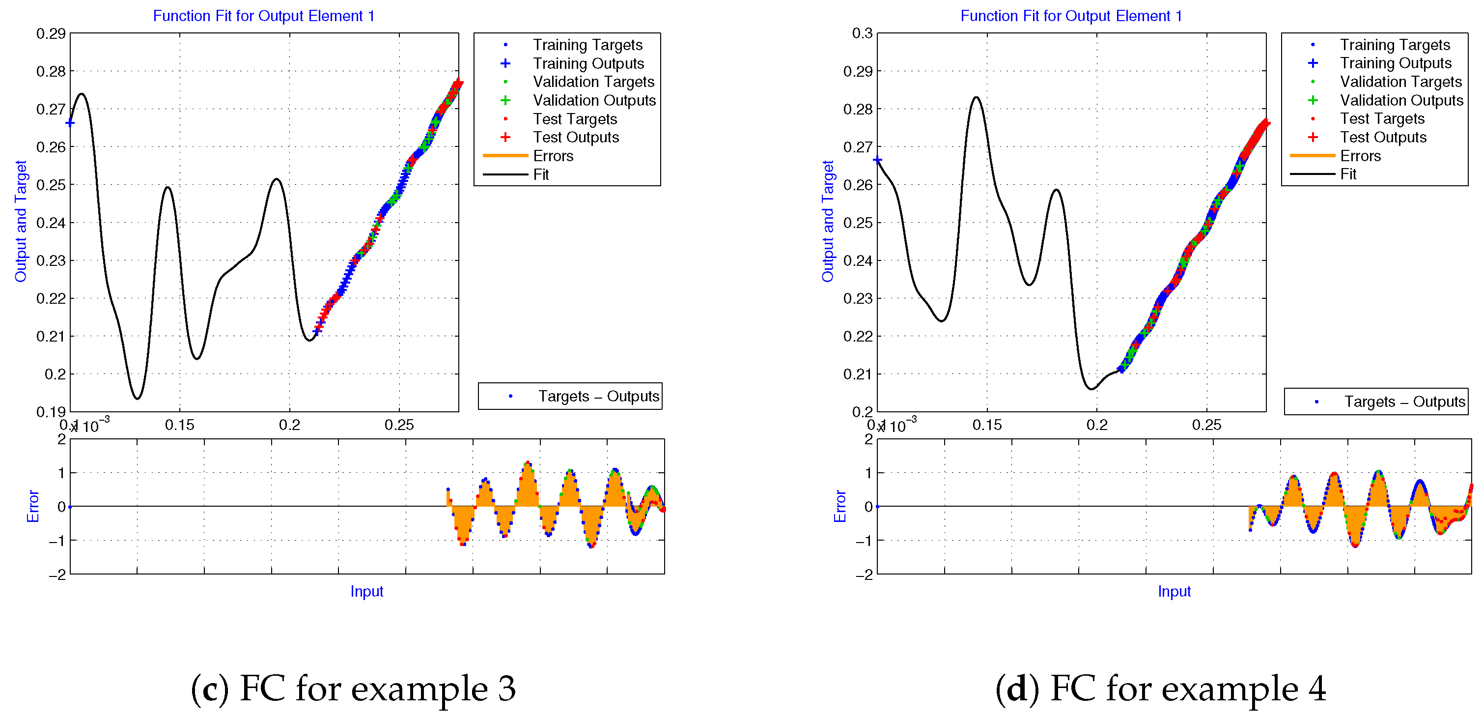
Table 17 displays the results of the inverse simultaneous methods based on artificial neural networks. The ANNs were trained using $70\%$ of the data set samples, with the remaining $30\%$ used to assess their ability to generalize using a performance metric. For a polynomial of degree 10, the ANN required 11 input data points, two hidden layers, and 22 output data points. In order to represent all the roots of engineering application 3, Figure 5c, Figure 6c, Figure 7c, Figure 8c, Figure 9c, display the EPH, MSE, RP, TS, and fitness overlapping graphs of the target and outcomes of the LMA-ANN algorithm for the training, testing, and validation. Table 17 provides a summary of the performance of ANNFN${}_{{\varsigma }_{1\ast }}$–ANNFN${}_{{\varsigma }_{5\ast }}$ in terms of the MSE, Per-E, Ex-time, and Error-it.

For training, testing, and validation, the input and output results of the LMA-ANNs’ fitness overlapping graphs are shown in Figure 5c. According to the histogram, the error is $6.43\times {10}^{-3}$, demonstrating the consistency of the suggested solver. For engineering application 3, the MSE of the LMA-ANNs compares the expected outcomes to the target solution, as shown in Figure 6c. The MSE for example 3 is $6.6649\times {10}^{-9}$ at epoch 112. The expected and actual results of the LMA-ANNs are linearly related, as shown in Figure 7c. Figure 8c illustrates the efficiency, consistency, and reliability of the engineering application 3 simulation. The gradient value is $9.9911\times {10}^{-6}$ with a Mu parameter of $1.0\times {10}^{-4}$. Figure 8c shows how the results for the minimal Mu and gradient converge closer as the network becomes more efficient in training and testing. The fitness curve and regression analysis results are displayed in Figure c. When R is near 1, the correlation parameter is close; however, it becomes unreliable when R is near 0. A reduced MSE causes a decreased response time.

The ANNs for various values of the fractional parameter, namely 0.1, 0.3, 0.5, 0.7, 0.8, and 1.0, are shown in Table 17 as ANNFN${}_{{\varsigma }_{1\ast }}$ through ANNFN${}_{{\varsigma }_{5\ast }}$.

The numerical results of the simultaneous schemes with initial guess values that vary close to the precise roots are shown in

Table 18. A comparison of the simultaneous schemes’ numerical results utilizing initial guess values that are close to the exact roots.

Method	WDKM	FINS${}_{\mathit{\varsigma }}$	ZPHM	MPCM	ANNFN${}_{{\mathit{\varsigma }}_{5\ast }}$	FINS${}_{{\mathit{\varsigma }}_{5\ast }}$
CPU Time	0.06334	0.05412	0.070018	0.06515	0.05002	0.01344
$e_1^{\left(\sigma \right)}$	$0.62\times {10}^{-4}$	$1.11\times {10}^{-23}$	$0.52\times {10}^{-30}$	$7.72\times {10}^{-48}$	$0.32\times {10}^{-20}$	$5.52\times {10}^{-67}$
$e_2^{\left(\sigma \right)}$	$0.01\times {10}^{-5}$	$9.15\times {10}^{-31}$	$9.91\times {10}^{-29}$	$0.17\times {10}^{-59}$	$0.17\times {10}^{-28}$	$8.18\times {10}^{-63}$
$e_3^{\left(\sigma \right)}$	$5.16\times {10}^{-4}$	$1.15\times {10}^{-14}$	$1.41\times {10}^{-31}$	$1.91\times {10}^{-35}$	$1.16\times {10}^{-36}$	$1.16\times {10}^{-64}$
$e_4^{\left(\sigma \right)}$	$0.15\times {10}^{-4}$	$5.13\times {10}^{-28}$	$7.31\times {10}^{-39}$	$0.61\times {10}^{-43}$	$3.71\times {10}^{-33}$	$3.71\times {10}^{-65}$
$e_5^{\left(\sigma \right)}$	$0.62\times {10}^{-5}$	$7.62\times {10}^{-24}$	$9.52\times {10}^{-35}$	$8.82\times {10}^{-45}$	$8.32\times {10}^{-27}$	$3.02\times {10}^{-65}$
$e_6^{\left(\sigma \right)}$	$4.51\times {10}^{-4}$	$9.15\times {10}^{-38}$	$3.91\times {10}^{-24}$	$4.17\times {10}^{-59}$	$6.16\times {10}^{-28}$	$6.16\times {10}^{-63}$
$e_7^{\left(\sigma \right)}$	$6.16\times {10}^{-4}$	$7.15\times {10}^{-14}$	$1.41\times {10}^{-38}$	$1.91\times {10}^{-38}$	$8.16\times {10}^{-38}$	$1.16\times {10}^{-64}$
$e_8^{\left(\sigma \right)}$	$7.15\times {10}^{-3}$	$3.13\times {10}^{-21}$	$0.31\times {10}^{-33}$	$3.61\times {10}^{-43}$	$3.71\times {10}^{-33}$	$3.71\times {10}^{-55}$
$e_9^{\left(\sigma \right)}$	$0.16\times {10}^{-4}$	$6.15\times {10}^{-14}$	$5.41\times {10}^{-38}$	$1.91\times {10}^{-38}$	$1.16\times {10}^{-38}$	$8.16\times {10}^{-68}$
$e_{10}^{\left(\sigma \right)}$	$9.99\times {10}^{-3}$	$3.13\times {10}^{-21}$	$3.31\times {10}^{-38}$	$3.61\times {10}^{-43}$	$3.71\times {10}^{-30}$	$3.88\times {10}^{-51}$
Max-Error	$6.10\times {10}^{-7}$	$0.13\times {10}^{-25}$	$3.31\times {10}^{-35}$	$0.01\times {10}^{-55}$	$4.71\times {10}^{-25}$	0.00
${\rho }^{\left(4\right)}$	1.844999	3.043114	5.013301	5.699912	3.4514245	6.010014

. In terms of the residual error, CPU time, and maximum error (Max-Error), our newly developed strategies surpass the existing methods on the same number of iterations.

Example 4

(Mechanical Engineering Application).

Mechanical engineering, like most other sciences, makes extensive use of thermodynamics [78]. The temperature of dry air is related to its zero-pressure specific heat, denoted as $C_{\rho }$, through the following polynomial:

$$C_{\rho }=1.9520\times {10}^{-14}{\upsilon }^4-9.5838\times {10}^{-11}{\upsilon }^3+9.7215\times {10}^{-8}{\upsilon }^2+1.671\times {10}^{-4}\upsilon +0.99403-1.2.$$

(51)

To calculate the temperature at which a heat capacity of, say, 1.2 kJ/kgK occurs, we replace $C_{r}ho=1.2$ in the equation above and obtain the following polynomial:

$$f_5\left(\upsilon \right)=1.9520\times {10}^{-14}{\upsilon }^4-9.5838\times {10}^{-11}{\upsilon }^3+9.7215\times {10}^{-8}{\upsilon }^2+1.671\times {10}^{-4}\upsilon -0.20597$$

(52)

with the exact roots

$$\begin{array}{ccc}\hfill {\zeta }_1& =& 1126.009751,{\zeta }_2=2536.837119+910.5010371i,{\zeta }_3=-1289.950382,\hfill \\ \hfill {\zeta }_4& =& 2536.837119-910.5010371i.\hfill \end{array}$$

The Caputo-type derivative of (52) is given as:

$$\begin{array}{ccc}\hfill \left[{}_C{⅁}_{{\varsigma }_1}^{\varsigma }\right]f_5\left(\upsilon \right)& =& 1.9520\times {10}^{-14}\frac{\lceil \left(5\right)}{\lceil (5-\varsigma )}{\upsilon }^{4-\varsigma }-9.5838\times {10}^{-11}\frac{\lceil \left(4\right)}{\lceil (4-\varsigma )}{\upsilon }^{3-\varsigma }+\hfill \\ & & 9.7215\times {10}^{-8}\frac{\lceil \left(3\right)}{\lceil (3-\varsigma )}{\upsilon }^{3-\varsigma }+1.671\times {10}^{-4}\frac{\lceil \left(2\right)}{\lceil (2-\varsigma )}{\upsilon }^{1-\varsigma }-\hfill \\ & & 0.20597\frac{1}{\lceil (9-\varsigma )}{\upsilon }^{-\varsigma },\hfill \end{array}$$

(53)

In order to quantify the global convergence rate of the inverse parallel fractional schemes FINS${}_{{\varsigma }_{1\ast }}$–FINS${}_{{\varsigma }_{5\ast }}$, a random initial guess value $v=[0.24,0.124,1.23,1.45.2.35]$ is generated by the built-in MATLAB rand() function. With a random initial estimate, FINS${}_{{\varsigma }_{1\ast }}$ converges to the exact roots after 9, 8, 7, 5, and 4 iterations and requires, respectively, 0.04164, 0.07144, 0.02514, 0.012017, and 0.015251 s to converge for different fractional parameters, namely 0.1, 0.3, 0.5, 0.8, and 1.0. The results in

Table 19. Approximation of all polynomial equation roots using FINS${\varsigma }_{1\ast }$–FINS${\varsigma }_{5\ast }$.

Method	${\mathit{e}}_1^{\left(\mathit{\sigma }\right)}$	${\mathit{e}}_2^{\left(\mathit{\sigma }\right)}$	${\mathit{e}}_3^{\left(\mathit{\sigma }\right)}$	${\mathit{e}}_4^{\left(\mathit{\sigma }\right)}$	${\mathit{\rho }}_{\mathit{\varsigma }\mathit{i}}^{(\mathit{\sigma }-1)}$	C-Time
$v=$ [0.24,0.124,1.23,1.45.2.35], Random initial approximations
FINS${}_{{\varsigma }_{1\ast }}$	$4.8\times {10}^{-31}$	$8.28\times {10}^{-31}$	$8.35\times {10}^{-31}$	$5.23\times {10}^{-31}$	$4.27\times {10}^{-31}$	n=16
FINS${}_{{\varsigma }_{2\ast }}$	$3.52\times {10}^{-31}$	$6.86\times {10}^{-29}$	$5.52\times {10}^{-32}$	$2.52\times {10}^{-31}$	$2.47\times {10}^{-30}$	0.1231
FINS${}_{{\varsigma }_{3\ast }}$	$8.28\times {10}^{-31}$	$5.25\times {10}^{-30}$	$8.8\times {10}^{-31}$	$6.52\times {10}^{-31}$	$6.46\times {10}^{-29}$	0.1023
FINS${}_{{\varsigma }_{4\ast }}$	$4.51\times {10}^{-26}$	$8.1\times {10}^{-26}$	$0.15\times {10}^{-26}$	$5.13\times {10}^{-26}$	$4.16\times {10}^{-26}$	0.1237
FINS${}_{{\varsigma }_{5\ast }}$	$1.1\times {10}^{-26}$	$1.1\times {10}^{-26}$	$1.1\times {10}^{-26}$	$1.1\times {10}^{-26}$	$1.1\times {10}^{-26}$	0.0012

clearly indicate that as the value of $\varsigma$ grows from 0.1 to 1.0, the rate of convergence of FINS${}_{{\varsigma }_{1\ast }}$ increases. Unlike ANNs, our newly developed algorithm converges to the exact roots for a range of random initial guesses, confirming a global convergence behavior. Figure 13a–e depict the root trajectories for various initial estimate values. When the initial approximation is close to the exact roots, the rate of convergence increases significantly, as illustrated in

Table 20. Approximation of all polynomial equation roots.

Method	FINS${}_{{\mathit{\varsigma }}_1}$	FINS${}_{{\mathit{\varsigma }}_2}$	FINS${}_{{\mathit{\varsigma }}_3}$	FINS${}_{{\mathit{\varsigma }}_4}$	FINS${}_{{\mathit{\varsigma }}_5}$
Error it	6	6	5	5	4
CPU	0.3141	0.316	0.167	0.0165	0.0111
$e_1^{\left(\sigma \right)}$	$5.2\times {10}^{-4}$	$3.32\times {10}^{-3}$	$0.3\times {10}^{-11}$	$7.2\times {10}^{-21}$	$7.2\times {10}^{-31}$
$e_2^{\left(\sigma \right)}$	$4.51\times {10}^{-2}$	$7.51\times {10}^{-3}$	$1.12\times {10}^{-16}$	$0.15\times {10}^{-26}$	$3.8\times {10}^{-46}$
$e_3^{\left(\sigma \right)}$	$1.61\times {10}^{-3}$	$2.31\times {10}^{-5}$	$1.16\times {10}^{-16}$	$1.17\times {10}^{-26}$	$6.9\times {10}^{-36}$
$e_4^{\left(\sigma \right)}$	$3.21\times {10}^{-3}$	$3.31\times {10}^{-6}$	$3.16\times {10}^{-16}$	$3.41\times {10}^{-36}$	$3.6\times {10}^{-56}$
${\rho }_{\varsigma i}^{(\sigma -1)}$	1.1212	2.2312	2.512	3.1412	3.2125

and

Table 21. Approximation of all polynomial equation roots.

Method	FINS${}_{{\mathit{\varsigma }}_{1\ast }}$	FINS${}_{{\mathit{\varsigma }}_{2\ast }}$	FINS${}_{{\mathit{\varsigma }}_{3\ast }}$	FINS${}_{{\mathit{\varsigma }}_{4\ast }}$	FINS${}_{{\mathit{\varsigma }}_{5\ast }}$
Error it	4	4	4	3	2
CPU	0.0141	0.016	0.054	0.067	0.065
$e_1^{\left(\sigma \right)}$	$0.2\times {10}^{-9}$	$0.2\times {10}^{-15}$	$0.2\times {10}^{-31}$	$0.2\times {10}^{-41}$	$0.2\times {10}^{-65}$
$e_2^{\left(\sigma \right)}$	$0.1\times {10}^{-7}$	$0.1\times {10}^{-13}$	$0.1\times {10}^{-26}$	$0.1\times {10}^{-46}$	$0.1\times {10}^{-66}$
$e_3^{\left(\sigma \right)}$	$1.1\times {10}^{-5}$	$1.1\times {10}^{-26}$	$1.1\times {10}^{-46}$	$1.1\times {10}^{-46}$	$1.1\times {10}^{-66}$
$e_4^{\left(\sigma \right)}$	$3.1\times {10}^{-5}$	$3.1\times {10}^{-16}$	$3.1\times {10}^{-26}$	$3.1\times {10}^{-46}$	$3.1\times {10}^{-69}$
${\rho }_{\varsigma i}^{(\sigma -1)}$	2.1212	3.2312	3.9123	4.5123	4.74123

.

The following initial guess value results in an increase in the convergence rates:

$$\stackrel{\left(0\right)}{{\upsilon }_1}=3,\stackrel{\left(0\right)}{{\upsilon }_2}=-1+1i,{\stackrel{\left(0\right)}{\upsilon }}_3=-0.1,{\stackrel{\left(0\right)}{\upsilon }}_4=-1+1i.$$

The initial estimates of (40) are as follows:

$$\stackrel{\left(0\right)}{{\upsilon }_1}=1126,\stackrel{\left(0\right)}{{\upsilon }_2}=2536+910i,{\stackrel{\left(0\right)}{\upsilon }}_3=-1289,{\stackrel{\left(0\right)}{\upsilon }}_4=2536-910i.$$

Table 22. Numerical results using artificial neural networks.

Methods	ANNFN${}_{{\mathit{\varsigma }}_{1\ast }}$	ANNFN${}_{{\mathit{\varsigma }}_{2\ast }}$	ANNFN${}_{{\mathit{\varsigma }}_{3\ast }}$	ANNFN${}_{{\mathit{\varsigma }}_{4\ast }}$	ANNFN${}_{{\mathit{\varsigma }}_{5\ast }}$
Error it	24	26	21	18	16
Ex-Time	1.45161	6.25412	4.06712	2.06545	3.07145
$e_1^{\left(\sigma \right)}$	$9.52\times {10}^{-4}$	$7.2\times {10}^{-3}$	$0.32\times {10}^{-11}$	$3.2\times {10}^{-11}$	$4.9\times {10}^{-11}$
$e_2^{\left(\sigma \right)}$	$7.1\times {10}^{-6}$	$6.51\times {10}^{-2}$	$0.31\times {10}^{-16}$	$0.67\times {10}^{-16}$	$9.1\times {10}^{-16}$
$e_3^{\left(\sigma \right)}$	$1.31\times {10}^{-3}$	$4.15\times {10}^{-3}$	$1.15\times {10}^{-16}$	$1.15\times {10}^{-16}$	$1.1\times {10}^{-16}$
$e_4^{\left(\sigma \right)}$	$3.1\times {10}^{-3}$	$3.15\times {10}^{-4}$	$3.13\times {10}^{-16}$	$3.17\times {10}^{-16}$	$3.1\times {10}^{-16}$
MSE	$3.1\times {10}^{-13}$	$3.15\times {10}^{-14}$	$3.13\times {10}^{-16}$	$3.17\times {10}^{-16}$	$3.1\times {10}^{-16}$
Per-E	99.31%	99.45%	96.45%	98.45%	96.87%

displays the results of the inverse simultaneous methods based on artificial neural networks. The ANNs were trained using $70\%$ of the data set samples, with the remaining $30\%$ used to assess their ability to generalize using a performance metric. For a polynomial of degree 4, the ANN required 5 input data points, two hidden layers, and 10 output data points. In order to represent all the roots of engineering application 4, Figure 5d, Figure 6d, Figure 7d, Figure 8d, Figure 9d, display the EPH, MSE, RP, TS, and fitness overlapping graphs of the target and outcomes of the LMA-ANN algorithm for the training, testing, and validation. Table 17 provides a summary of the performance of ANNFN${}_{{\varsigma }_{1\ast }}$–ANNFN${}_{{\varsigma }_{5\ast }}$ in terms of the MSE, Per-E, Ex-time, and Error-it.

For training, testing, and validation, the input and output results of the LMA-ANNs’ fitness overlapping graphs are shown in Figure 5d. According to the histogram, the error is 1.08$\times {10}^{-6}$, demonstrating the consistency of the suggested solver. For engineering application 4, the MSE of the LMA-ANNs compares the expected outcomes to the target solution, as shown in Figure 6d. The MSE for example 4 is $6.0469\times {10}^{-9}$ at epoch 49. The expected and actual results of the LMA-ANNs are linearly related, as shown in Figure 7d. Figure 8d illustrates the efficiency, consistency, and reliability of the engineering application 4 simulation. The gradient value is 3.0416$\times {10}^{-4}$ with a Mu parameter of 1.0$\times {10}^{-6}$. Figure 8d shows how the results for the minimal Mu and gradient converge closer as the network becomes more efficient in training and testing. The fitness curve and regression analysis results are displayed in Figure d. When R is near 1, the correlation parameter is close; however, it becomes unreliable when R is near 0. A reduced MSE causes a decreased response time.

The ANNs for various values of the fractional parameter, namely 0.1, 0.3, 0.5, 0.7, 0.8, and 1.0, are shown in Table 22 as ANNFN${}_{{\varsigma }_{1\ast }}$ through ANNFN${}_{{\varsigma }_{5\ast }}$.

Table 23. A comparison of the numerical results of the simultaneous schemes utilizing initial guess values that are close to the exact roots.

Method	WDKM	FINS${}_{\mathit{\varsigma }}$	ZPHM	MPCM	ANNFN${}_{{\mathit{\varsigma }}_{5\ast }}$	FINS${}_{{\mathit{\varsigma }}_{5\ast }}$
CPU Time	0.05414	0.03004	0.07178	0.04085	0.03151	0.01554
$e_1^{\left(5\right)}$	$6.62\times {10}^{-4}$	$8.62\times {10}^{-24}$	$9.52\times {10}^{-35}$	$8.82\times {10}^{-45}$	$0.32\times {10}^{-27}$	$3.32\times {10}^{-65}$
$e_2^{\left(5\right)}$	$4.51\times {10}^{-4}$	$1.15\times {10}^{-35}$	$9.91\times {10}^{-24}$	$0.17\times {10}^{-59}$	$0.16\times {10}^{-28}$	$6.16\times {10}^{-63}$
$e_3^{\left(5\right)}$	$0.16\times {10}^{-4}$	$7.15\times {10}^{-14}$	$1.41\times {10}^{-38}$	$0.91\times {10}^{-38}$	$1.16\times {10}^{-38}$	$1.11\times {10}^{-64}$
$e_4^{\left(5\right)}$	$3.15\times {10}^{-3}$	$3.13\times {10}^{-21}$	$3.31\times {10}^{-33}$	$3.61\times {10}^{-43}$	$3.71\times {10}^{-33}$	$3.71\times {10}^{-65}$
Max-Error	$6.15\times {10}^{-7}$	$9.13\times {10}^{-25}$	$3.31\times {10}^{-35}$	$0.61\times {10}^{-55}$	$4.71\times {10}^{-25}$	0.00
${\rho }^{\left(4\right)}$	1.944125	3.013554	5.014512	5.812312	3.5514245	6.0144247

presents the numerical results of the simultaneous schemes when the initial guess values approach the exact roots. When evaluating the same number of iterations, our newly devised strategies outperform the existing methods in terms of the maximum error (Max-Error), residual error, and CPU time. When evaluating the same number of iterations, our newly proposed strategies outperform the existing methods in terms of the residual error, CPU time, and maximum error (Max-Error).

The root trajectories of the nonlinear equations arising from engineering applications 1–4 clearly demonstrate that our FINS${}_{{\varsigma }_{1\ast }}$–FINS${}_{{\varsigma }_{5\ast }}$ schemes converge to the exact roots starting from random initial guesses, and the rate of convergence increases as the value of $\varsigma$ increases from 0.1 to 1.0.

8. Conclusions

In this research, two new fractional inverse simultaneous schemes of convergence orders $\varsigma +2$ and $2\varsigma +4$ are presented to approximate all nonlinear equation roots. Some engineering applications are solved for various random initial approximations to demonstrate the global convergence of the newly developed fractional schemes. In order to prove the claim of global convergence, dynamical planes and root trajectories are generated, as shown in Figure 3a,b, Figure 10a–e, Figure 11a–e, Figure 12a–e, Figure 13a–e, and Table 4, Table 9, Table 14, and Table 19. In Table 2 and Table 3, the elapsed time, percentage convergence, and divergence points of the dynamical planes generated by FINS${}_{{\varsigma }_1}$–FINS${}_{{\varsigma }_5}$ and FINS${}_{{\varsigma }_{1\ast }}$–FINS${}_{{\varsigma }_{5\ast }}$ demonstrate the efficiency and stability of the new class of root-finding methods. As demonstrated in Table 5, Table 6, Table 8, Table 10, Table 11, Table 13, Table 15, Table 16, Table 18, Table 20, Table 21, and Table 23, the rate of convergence increases when we choose initial guesses that are close to the exact root.

The ANNs were initially trained using the LMA technique and the coefficients of the examined polynomials. The differences between the values generated by each ANN, i.e., the polynomial root estimations and the values of the exact roots, were used to adjust the weights of each ANN. The results in Table 7, Table 12, Table 17, and Table 21 show that ANNFN${}_{{\varsigma }_{1\ast }}$–ANNFN${}_{{\varsigma }_{5\ast }}$ outperformed the conventional ANNs in terms of accuracy. For the various fractional parameter values, the FINS${}_{{\varsigma }_1}$–FINS${}_{{\varsigma }_5}$, FINS${}_{{\varsigma }_{1\ast }}$–FINS${}_{{\varsigma }_{5\ast }}$, and ANNFN${}_{{\varsigma }_{1\ast }}$–ANNFN${}_{{\varsigma }_{5\ast }}$ methods exhibited better performance compared to other existing root-finding methods, such as WDKM, ZPHM, and MPCM, in terms of computational efficiency, order of convergence, residual error, elapsed time, MSE, and percentage convergence rate (see, e.g., Table 4, Table 5, Table 6, Table 7, Table 8, Table 9, Table 10, Table 11, Table 12, Table 13, Table 14, Table 15, Table 16, Table 17, Table 18, Table 19, Table 20, Table 21, Table 22 and Table 23).

Further studies will focus on developing higher-order inverse fractional simultaneous iterative methods for computing all nonlinear equation roots that arise in more complex engineering applications [79,80,81].

References

1. Alekseev, V.B. Abel’s Theorem in Problems and Solutions: Based on the Lectures of Professor VI Arnold; Springer: Dordrecht, The Netherlands, 2004. [Google Scholar]
2. Sjogren, J.A.; Li, X.; Zhao, M.; Lu, C. Computable implementation of “Fundamental Theorem of Algebra”. Int. J. Pure Appl. Math. 2013, 86, 95–131. [Google Scholar] [CrossRef]
3. Consnard, M.; Fraigniaud, P. Finding the roots of a polynomial on an MIMD multicomputer. Parallel Comput. 1990, 15, 75–85. [Google Scholar] [CrossRef]
4. Chun, C.; Kim, Y.I. Several new third-order iterative methods for solving nonlinear equations. Acta Appl. Math. 2010, 109, 1053–1063. [Google Scholar] [CrossRef]
5. Madhu, K.; Jayaraman, J. Higher order methods for nonlinear equations and their basins of attraction. Mathematics 2016, 4, 22. [Google Scholar] [CrossRef]
6. Kiran, R.; Khandelwal, K. On the application of multipoint Root-Solvers for improving global convergence of fracture problems. Eng. Fract. Mech. 2018, 193, 77–95. [Google Scholar] [CrossRef]
7. Weierstrass, K. Neuer Beweis des Satzes, dass jede ganze rationale Function einer Verän derlichen dargestellt werden kann als ein Product aus linearen Functionen derselben Verän derlichen. Sitzungsberichte KöNiglich Preuss. Akad. Der Wiss. Berl. 1981, 2, 1085–1101. [Google Scholar]
8. Kerner, I.O. Ein gesamtschrittverfahren zur berechnung der nullstellen von polynomen. Numer. Math. 1966, 8, 290–294. [Google Scholar] [CrossRef]
9. Durand, E. Solutions numériques des équations algébriques: Systèmes de plusieurs équations. Val. Propres Matrices Masson 1962, 2, 1–10. [Google Scholar]
10. Dochev, M. Modified Newton method for the simultaneous computation of all roots of a given algebraic equation. Phys. Math. J. Bulg. Acad. Sci. 1962, 5, 136–139. (In Bulgarian) [Google Scholar]
11. Presic, S. Un procédé itératif pour la factorisation des polynômes. CR Acad. Sci. Paris 1966, 262, 862–863. [Google Scholar]
12. Alefeld, G.; Herzberger, J. On the convergence speed of some algorithms for the simultaneous approximation of polynomial roots. SIAM J. Numer. Anal. 1974, 11, 237–243. [Google Scholar] [CrossRef]
13. Petkovic, M. Iterative methods for simultaneous inclusion of polynomial zeros. Lect. Notes Math. 1989, 1387, X-263. [Google Scholar]
14. Börsch-Supan, W. Residuenabschätzung für Polynom-Nullstellen mittels Lagrange-Interpolation. Numer. Math. 1970, 14, 287–296. [Google Scholar] [CrossRef]
15. Rafiq, N.; Mir, N.A.; Yasmin, N. Some two-step simultaneous methods for determining all the roots of a non-linear equation. Life Sci. J. 2013, 10, 54–59. [Google Scholar]
16. Proinov, P.D.; Petkova, M.D. Convergence of the two-point Weierstrass root-finding method. Jpn. J. Ind. Appl. Math. 2014, 31, 279–292. [Google Scholar] [CrossRef]
17. Zhang, X.; Peng, H.; Hu, G. A high order iteration formula for the simultaneous inclusion of polynomial zeros. Appl. Math. Comput. 2006, 179, 545–552. [Google Scholar] [CrossRef]
18. Aberth, O. Iteration methods for finding all zeros of a polynomial simultaneously. Math. Comput. 1973, 27, 339–344. [Google Scholar] [CrossRef]
19. Milovanovic, G.V.; Petkovic, M.S. On computational efficiency of the iterative methods for the simultaneous approximation of polynomial zeros. ACM Trans. Math. Softw. 1986, 12, 295–306. [Google Scholar] [CrossRef]
20. Nourein, A.W. An improvement on Nourein’s method for the simultaneous determination of the zeroes of a polynomial (an algorithm). J. Comput. Appl. Math. 1977, 3, 109–112. [Google Scholar] [CrossRef]
21. Petković, M.S.; Petković, L.D.; Džunić, J. On an efficient method for the simultaneous approximation of polynomial multiple roots. Appl. Anal. Discrete Math. 2014, 8, 73–94. [Google Scholar] [CrossRef]
22. Farmer, M.R. Computing the Zeros of Polynomials Using the Divide and Conquer Approach; Department of Computer Science and Information Systems, Birkbeck, University of London: London, UK, 2014. [Google Scholar]
23. Proinov, P.D. General convergence theorems for iterative processes and applications to the Weierstrass root-finding method. J. Complex. 2016, 33, 118–144. [Google Scholar] [CrossRef]
24. Nedzhibov, G.H. Improved local convergence analysis of the Inverse Weierstrass method for simultaneous approximation of polynomial zeros. In Proceedings of the MATTEX 2018 Conference, Targovishte, Bulgaria, 16–17 November 2018; Volume 1, pp. 66–73. [Google Scholar]
25. Marcheva, P.I.; Ivanov, S.I. Convergence analysis of a modified Weierstrass method for the simultaneous determination of polynomial zeros. Symmetry 2020, 12, 1408. [Google Scholar] [CrossRef]
26. Shams, M.; Ahmad Mir, N.; Rafiq, N.; Almatroud, A.O.; Akram, S. On dynamics of iterative techniques for nonlinear equation with applications in engineering. Math. Probl. Eng. 2020, 2020, 5853296. [Google Scholar] [CrossRef]
27. Shams, M.; Rafiq, N.; Kausar, N.; Agarwal, P.; Park, C.; Mir, N.A. On iterative techniques for estimating all roots of nonlinear equation and its system with application in differential equation. Adv. Differ. Equ. 2021, 2021, 480. [Google Scholar] [CrossRef]
28. Shams, M.; Rafiq, N.; Kausar, N.; Agarwal, P.; Mir, N.A.; Li, Y.M. On Highly Efficient Simultaneous Schemes for Finding all Polynomial Roots. Fractals 2022, 30, 2240198. [Google Scholar] [CrossRef]
29. Chinesta, F.; Cordero, A.; Garrido, N.; Torregrosa, J.R.; Triguero-Navarro, P. Simultaneous roots for vectorial problems. Comput. Appl. Math. 2023, 42, 227. [Google Scholar] [CrossRef]
30. Triguero Navarro, P. High Performance Multidimensional Iterative Processes for Solving Nonlinear Equations. Doctoral Dissertation, Universitat Politècnica de València, València, Spain, 2023. [Google Scholar]
31. Luk, W.S. Finding roots of a real polynomial simultaneously by means of Bairstow’s method. BIT Numer. Math. 1996, 36, 302–308. [Google Scholar] [CrossRef]
32. Cholakov, S.I. Local and semilocal convergence of Wang-Zheng’s method for simultaneous finding polynomial zeros. Symmetry 2019, 11, 736. [Google Scholar] [CrossRef]
33. Mir, N.A.; Shams, M.; Rafiq, N.; Akram, S.; Rizwan, M. Derivative free iterative simultaneous method for finding distinct roots of polynomial equation. Alex. Eng. J. 2020, 59, 1629–1636. [Google Scholar] [CrossRef]
34. Gdawiec, K.; Kotarski, W.; Lisowska, A. Newton’s method with fractional derivatives and various iteration processes via visual analysis. Numer. Algorithms 2021, 86, 953–1010. [Google Scholar] [CrossRef]
35. Bayrak, M.A.; Demir, A.; Ozbilge, E. On fractional Newton-type method for nonlinear problems. J. Math. 2022, 2022, 7070253. [Google Scholar] [CrossRef]
36. Odibat, Z.M.; Shawagfeh, N.T. Generalized Taylor’s formula. Appl. Math. Comput. 2007, 186, 286–293. [Google Scholar] [CrossRef]
37. Akgül, A.; Cordero, A.; Torregrosa, J.R. A fractional Newton method with α-th order of convergence and its stability. Appl. Math. Lett. 2019, 98, 344–351. [Google Scholar] [CrossRef]
38. Torres-Hernandez, A.; Brambila-Paz, F. Sets of fractional operators and numerical estimation of the order of convergence of a family of fractional fixed-point methods. Fractal Fract. 2021, 5, 240. [Google Scholar] [CrossRef]
39. Cajori, F. Historical note on the Newton-Raphson method of approximation. Am. Math. Mon. 1911, 18, 29–32. [Google Scholar] [CrossRef]
40. Kumar, P.; Agrawal, O.P. An approximate method for numerical solution of fractional differential equations. Signal Process. 2006, 86, 2602–2610. [Google Scholar] [CrossRef]
41. Candelario, G.; Cordero, A.; Torregrosa, J.R. Multipoint fractional iterative methods with (2α + 1)th-order of convergence for solving nonlinear problems. Mathematics 2020, 8, 452. [Google Scholar] [CrossRef]
42. Shams, M.; Kausar, N.; Agarwal, P.; Oros, G.I. Efficient iterative scheme for solving non-linear equations with engineering applications. Appl. Math. Sci. Eng. 2022, 30, 708–735. [Google Scholar] [CrossRef]
43. Attary, M.; Agarwal, P. On developing an optimal Jarratt-like class for solving nonlinear equations. Forum-Ed. Udinese SRL 2020, 43, 523–530. [Google Scholar]
44. Akram, S.; Akram, F.; Junjua, M.U.D.; Arshad, M.; Afzal, T. A family of optimal Eighth order iteration functions for multiple roots and its dynamics. J. Math. 2021, 2021, 5597186. [Google Scholar] [CrossRef]
45. Cordero, A.; Neta, B.; Torregrosa, J.R. Memorizing Schröder’s method as an efficient strategy for estimating roots of unknown multiplicity. Mathematics 2021, 9, 2570. [Google Scholar] [CrossRef]
46. Shams, M.; Rafiq, N.; Kausar, N.; Agarwal, P.; Park, C.; Mir, N.A. On highly efficient derivative-free family of numerical methods for solving polynomial equation simultaneously. Adv. Differ. Equ. 2021, 2021, 465. [Google Scholar] [CrossRef]
47. Shams, M.; Rafiq, N.; Kausar, N.; Agarwal, P.; Mir, N.A.; El-Kanj, N. On Inverse Iteration process for finding all roots of nonlinear equations with applications. Fractals 2022, 30, 2240265. [Google Scholar] [CrossRef]
48. Rafiq, N.; Akram, S.; Shams, M.; Mir, N.A. Computer geometries for finding all real zeros of polynomial equations simultaneously. Comput. Mater. Contin. 2021, 69, 2636–2651. [Google Scholar] [CrossRef]
49. Nedzhibov, G.H. On semilocal convergence analysis of the Inverse Weierstrass method for simultaneous computing of polynomial zeros. Ann. Acad. Rom. Sci. Ser. Math. Appl. 2019, 11, 247–258. [Google Scholar]
50. Proinov, P.D.; Petkova, M.D. Local and semilocal convergence of a family of multi-point Weierstrass-type root-finding methods. Mediterr. J. Math. 2020, 17, 107. [Google Scholar] [CrossRef]
51. Shams, M.; Rafiq, N.; Ahmad, B.; Mir, N.A. Inverse numerical iterative technique for finding all roots of nonlinear equations with engineering applications. J. Math. 2021, 2021, 6643514. [Google Scholar] [CrossRef]
52. Hormis, R.; Antoniou, G.; Mentzelopoulou, S. Separation of two-dimensional polynomials via a sigma-pi neural net. In Proceedings of the IASTED International Conference Modelling and Simulation, Colombo, Sri Lanka, 26–28 July 1995; pp. 304–306. [Google Scholar]
53. Huang, D.S.; Chi, Z. Finding complex roots of polynomials by feedforward neural networks. In Proceedings of the IJCNN’01. International Joint Conference on Neural Networks, Cat. No. 01CH37222, Washington, DC, USA, 15–19 July 2001; p. A13. [Google Scholar]
54. Huang, D.S.; Chi, Z. Neural networks with problem decomposition for finding real roots of polynomials. In Proceedings of the IJCNN’01. International Joint Conference on Neural Networks, (Cat. No. 01CH37222), Washington, DC, USA, 15–19 July 2001; p. A25. [Google Scholar]
55. Huang, D.S.; Ip, H.H.; Chi, Z.; Wong, H.S. Dilation method for finding close roots of polynomials based on constrained learning neural networks. Phys. Lett. A 2003, 309, 443–451. [Google Scholar] [CrossRef]
56. Huang, D.S. A constructive approach for finding arbitrary roots of polynomials by neural networks. IEEE Trans. Neural Netw. 2004, 15, 477–491. [Google Scholar] [CrossRef]
57. Levenberg, K. A method for the solution of certain non-linear problems in least squares. Q. Appl. Math. 1944, 2, 164–168. [Google Scholar] [CrossRef]
58. Marquardt, D.W. An algorithm for least-squares estimation of nonlinear parameters. SIAM J. Appl. Math. 1963, 11, 431–441. [Google Scholar] [CrossRef]
59. Hagan, M.T.; Menhaj, M.B. Training feedforward networks with the Marquardt algorithm. IEEE Trans. Neural Netw. 1994, 5, 989–993. [Google Scholar] [CrossRef]
60. Hagan, M.T.; Demuth, H.B.; Beale, M. Neural Network Design; PWS Publishing Co.: Boston, MA, USA, 1997. [Google Scholar]
61. Heaton, J. Artificial Intelligence for Humans: Deep Learning and Neural; Heaton Research, Incorporated: Chesterfield, UK, 2015. [Google Scholar]
62. Shams, M.; Rafiq, N.; Kausar, N.; Agarwal, P.; Park, C.; Momani, S. Efficient iterative methods for finding simultaneously all the multiple roots of polynomial equation. Adv. Differ. Equ. 2021, 2021, 495. [Google Scholar] [CrossRef]
63. Proinov, P.D. On the local convergence of Gargantini-Farmer-Loizou method for simultaneous approximation of multiple polynomial zeros. J. Nonlinear Sci. Appl. 2018, 11, 1045–1055. [Google Scholar] [CrossRef]
64. Mir, N.A.; Shams, M.; Rafiq, N.; Akram, S.; Ahmed, R. On Family of Simultaneous Method for Finding Distinct as Well as Multiple Roots of Non-linear Equation. Punjab Univ. J. Math. 2020, 52, 31–44. [Google Scholar]
65. Petković, M.S.; Petković, L.D.; Džunić, J. On an efficient simultaneous method for finding polynomial zeros. Appl. Math. Lett. 2014, 28, 60–65. [Google Scholar] [CrossRef]
66. Kung, H.T.; Traub, J.F. Optimal order of one-point and multipoint iteration. J. ACM 1974, 21, 643–651. [Google Scholar] [CrossRef]
67. Dong, C. A family of multiopoint iterative functions for finding multiple roots of equations. Int. J. Comput. Math. 1987, 21, 363–367. [Google Scholar] [CrossRef]
68. Scott, M.; Neta, B.; Chun, C. Basin attractors for various methods. Appl. Math. Comput. 2011, 218, 2584–2599. [Google Scholar] [CrossRef]
69. Chicharro, F.; Cordero, A.; Gutiérrez, J.M.; Torregrosa, J.R. Complex dynamics of derivative-free methods for nonlinear equations. Appl. Math. Comput. 2013, 219, 7023–7035. [Google Scholar] [CrossRef]
70. Pulvirenti, G.; Faria, C. Influence of Housing Wall Compliance on Shock Absorbers in the Context of Vehicle Dynamics. IOP Conf. Ser. Mater. Sci. Eng. 2017, 252, 012026. [Google Scholar] [CrossRef]
71. Konieczny, L. Analysis of simplifications applied in vibration damping modelling for a passive car shock absorber. Shock Vib. 2016, 2016, 6182847. [Google Scholar] [CrossRef]
72. Liu, Y.; Zhang, J. Nonlinear dynamic responses of twin-tube hydraulic shock absorber. Mech. Res. Commun. 2002, 29, 359–365. [Google Scholar] [CrossRef]
73. Barethiye, V.M.; Pohit, G.; Mitra, A. Analysis of a quarter car suspension system based on nonlinear shock absorber damping models. Int. J. Automot. Mech. 2017, 14, 4401–4418. [Google Scholar] [CrossRef]
74. Ali, B.A.; Salit, M.S.; Zainudin, E.S.; Othman, M. Integration of artificial neural network and expert system for material classification of natural fibre reinforced polymer composites. Am. J. Appl. Sci. 2015, 12, 174. [Google Scholar]
75. Fournier, R.L. Basic Transport Phenomena in Biomedical Engineering; Taylor & Franics: New York:, NY, USA, 2007. [Google Scholar]
76. Bronshtein, I.N.; Semendyayev, K.A. Handbook of Mathematics; Springer Science & Business Media: Berlin/Heidelberg, Germany, 2013. [Google Scholar]
77. Polyanin, A.D.; Manzhirov, A.V. Handbook of Mathematics for Engineers and Scientists; CRC Press: Boca Raton, FL, USA, 2006. [Google Scholar]
78. Chu, Y.; Rafiq, N.; Shams, M.; Akram, S.; Mir, N.A.; Kalsoom, H. Computer methodologies for the comparison of some efficient derivative free simultaneous iterative methods for finding roots of non-linear equations. Comput. Mater. Contin. 2020, 66, 275–290. [Google Scholar] [CrossRef]
79. Shams, M.; Kausar, N.; Samaniego, C.; Agarwal, P.; Ahmed, S.F.; Momani, S. On Efficient Fractional Caputo-type Simultaneous Scheme for Finding all Roots of Polynomial Equations with Biomedical Engineering Applications. Fractals 2023, 2340075. [Google Scholar] [CrossRef]
80. Jay, L.O. A note on Q-order of convergence. BIT Numer. Math. 2001, 41, 422–429. [Google Scholar] [CrossRef]
81. Argyros, I.K.; Magreñán, Á.A.; Orcos, L. Local convergence and a chemical application of derivative free root finding methods with one parameter based on interpolation. J. Math. Chem. 2016, 54, 1404–1416. [Google Scholar] [CrossRef]
Figure 1. A schematic representation of the process of feeding the coefficients of a polynomial into an ANN, which then yields an approximation for each root of (1).
Fractalfract 07 00849 g001
Figure 2. (ae) Computational efficiency of FINS ς 1 –FINS ς 5 in comparison to the IWDKI method. (a) Computational efficiency of FINS ς 1 in comparison to the IWDKI method. (b) Computational efficiency of FINS ς 2 in comparison to the IWDKI method. (c) Computational efficiency of FINS ς 3 in comparison to the IWDKI method. (d) Computational efficiency of FINS ς 4 in comparison to the IWDKI method. (e) Computational efficiency of FINS ς 5 in comparison to the IWDKI method.
Fractalfract 07 00849 g002aFractalfract 07 00849 g002b
Figure 3. (a,b) Basins of attraction of the FINS ς 1 –FINS ς 5 and FINS ς 1 –FINS ς 5 methods for various values of ς . (a) Attraction basins of FINS ς 1 –FINS ς 5 for various values of ς . (b) Attraction basins of FINS ς 1 –FINS ς 5 for various values of ς .
Fractalfract 07 00849 g003
Figure 4. Model of a quarter car.
Fractalfract 07 00849 g004
Figure 5. (ad) LMA-ANNs are utilized to represent error histograms (EHP), which are subsequently used to approximate the roots of the polynomial equations used in engineering applications 1–4. According to the histograms, the errors are approximately 6.2 × 10 2 , 0.51, 6.43 × 10 3 , and 1.08 × 10 6 , respectively. These graphs demonstrate the consistency of the proposed solver.
Fractalfract 07 00849 g005
Figure 6. (ad) Mean square error (MSE) of the LMA-ANN methods utilized to approximate each root of the polynomial equations in engineering applications 1–4. The best outcomes are achieved at epochs 112, 49, 112, and 49, with MSE values of 6.6649 × 10 9 , 1.1914 × 10 9 , 6.1914 × 10 9 , and 1.0469 × 10 9 , respectively. A small MSE suggests a good match between the target solutions and expected outcomes.
Fractalfract 07 00849 g006
Figure 7. (ad) Regression plots (RPs) for LMA-ANN methods utilized to approximate the roots of the polynomial equations. Regression diagrams show the linear relationship between the expected and actual outcomes. The visualizations include all of the training, validation, and test data. The data exhibit the highest degree of correlation with a curve or line when the regression value is R = 1 [74].
Fractalfract 07 00849 g007
Figure 8. (ad) Transition statistics (TS) for the LMA-ANN methods utilized to approximate the roots of the polynomial equations. Statistical results for engineering models 1–4 are shown in (ad). The gradient values are 9.9314 × 10 6 , 9.8016 × 10 6 , 9.9911 × 10 6 , 3.0416 × 10 4 and the Mu values are 1.0 × 10 4 , 1.0 × 10 5 , 1.0 × 10 4 , 1.0 × 10 6 for all four examples. The results of the transition statistics reflect the effective convergence rate of the LMA-ANNs. The gradient and Mu should be set to their lowest values for convergence to occur.
Fractalfract 07 00849 g008
Figure 9. (ad) Fitness curves (FCs) for the LMA-ANN methods utilized to approximate the roots of Equation (1). The way the fitness curves overlap demonstrates the accuracy and stability of the methods.
Fractalfract 07 00849 g009aFractalfract 07 00849 g009b
Figure 10. (ae) Root trajectories of the inverse fractional numerical schemes used in engineering application 1 for approximating all roots of polynomial equations for various fractional parameter values, namely ς = 0.1 , 0.3 , 0.7 , 0.8 , 1.0 . (a) Root trajectory for parameter = 0.1. (b) Root trajectory for parameter = 0.3. (c) Root trajectory for parameter = 0.7. (d) Root trajectory for parameter = 0.8. (e) Root trajectory for parameter = 1.0.
Fractalfract 07 00849 g010
Figure 11. (ae) Root trajectories of the inverse fractional numerical schemes used in engineering application 2 for approximating all roots of polynomial equations for various fractional parameter values, namely ς = 0.1 , 0.3 , 0.7 , 0.8 , 1.0 . (a) Root trajectory for parameter = 0.1. (b) Root trajectory for parameter = 0.3. (c) Root trajectory for parameter = 0.7. (d) Root trajectory for parameter = 0.8. (e) Root trajectory for parameter = 1.0.
Fractalfract 07 00849 g011
Figure 12. (ae) Root trajectories of the inverse fractional numerical schemes used in engineering application 3 for approximating all roots of polynomial equations for various fractional parameter values, namely ς = 0.1 , 0.3 , 0.7 , 0.8 , 1.0 . (a) Root trajectory for parameter = 0.1. (b) Root trajectory for parameter = 0.3. (c) Root trajectory for parameter = 0.7. (d) Root trajectory for parameter = 0.8. (e) Root trajectory for parameter = 1.0.
Fractalfract 07 00849 g012
Figure 13. (ae) Root trajectories of the inverse fractional numerical schemes used in engineering application 4 for approximating all roots of polynomial equations for various fractional parameter values, namely ς = 0.1 , 0.3 , 0.7 , 0.8 , 1.0 . (a) Root trajectory for parameter = 0.1. (b) Root trajectory for parameter = 0.3. (c) Root trajectory for parameter = 0.7. (d) Root trajectory for parameter = 0.8. (e) Root trajectory for parameter = 1.0.
Fractalfract 07 00849 g013