Dynamical Analysis and SDEPINN-Based Modeling of a Fractional-Order Stochastic SIS Epidemic Model

Abstract

This paper proposes a novel susceptible–infected–susceptible (SIS) epidemic model incorporating a fractional-order term and white-noise perturbations. Several analytical results concerning its dynamical behavior are established. Firstly, we prove the existence and uniqueness of model solutions using the Carathéodory approximation. Secondly, the extinction of disease is rigorously proven based on the properties of the quadratic function. Meanwhile, the Ulam–Hyers stability of the model is derived by using stochastic Gronwall-type inequalities and the stochastic analysis techniques. Furthermore, the solution of the proposed fractional-order stochastic model can be approximated by that of the corresponding averaged model under suitable averaging conditions. Then, numerical simulations are conducted to illustrate the effects of key parameters on disease extinction, stability, and long-term dynamical behavior. To improve its adaptability to real-world epidemic dynamics, this paper embeds dynamical constraints into neural networks and constructs a stochastic physics-informed identification framework for seasonal infectious diseases. Empirical results based on monthly influenza data from Xinjiang show that the proposed framework can capture epidemic trends, seasonal peaks, and fitting uncertainty. These results provide a theoretically grounded and practically applicable approach for infectious disease modeling under memory effects and stochastic perturbations.

1. Introduction

In epidemiological research and public health practice, dynamical models provide an indispensable quantitative tool for analyzing infectious disease transmission. Deterministic models have long served as a fundamental paradigm for understanding the mechanisms of disease spread [1,2]. However, different infectious diseases often exhibit substantial differences in transmission modes, immune mechanisms, and epidemiological characteristics, which requires the model structure to be carefully matched with the specific features of the disease under consideration.

For certain infectious diseases, such as seasonal influenza, cytomegalovirus infection, and tuberculosis, recovered individuals may return to the susceptible state due to the loss or waning of immunity. In particular, the transmission dynamics of seasonal influenza depend not only on the current infection status of the population, but are also strongly influenced by memory effects such as immune waning and previous infection history. The SIS model provides a basic framework for describing such reinfection mechanisms [3,4,5]. To incorporate more complex nonlinear contact mechanisms, the deterministic SIS model with a general incidence function can be formulated as follows:

$$\left\{\begin{array}{c}dS\left(t\right)=[\Lambda -\theta S(t)-\beta f(S\left(t\right),I\left(t\right))+\gamma I(t\left)\right]dt,\hfill \\ dI\left(t\right)=\left[\beta f\right(S\left(t\right),I\left(t\right))-(\theta +\gamma \left)I\right(t\left)\right]dt,\hfill \end{array}\right.$$

(1)

where $S\left(t\right)$ and $I\left(t\right)$ represent the number of susceptible and infectious individuals at time t, respectively. Parameter $\Lambda$ is the birth rate, $\theta$ is the natural death rate, $\beta$ is the effective contact rate, and $\gamma$ is the recovery rate of the infectious individual. In the model (1), suppose that the function $f\left(S\right(t),I(t\left)\right)$ is continuously differentiable. Compared with deterministic models, stochastic models are generally better able to capture individual variations, stochastic events, and transmission in small populations [6,7,8,9,10]. There are considerable works about stochastic perturbations acting on the effective contact rate $\beta$, as in [11,12,13,14], $\beta \to \beta +{\sigma }_{1}B\left(t\right)$, where $B\left(t\right)$ is standard Brownian motion with $B\left(0\right)=0$, and ${\sigma }_1$ is the intensity. Hence, the stochastic version of model (1) is formed by:

$$\left\{\begin{array}{c}dS\left(t\right)=[\Lambda -\theta S\left(t\right)-\beta f(S\left(t\right),I\left(t\right))+\gamma I\left(t\right)]dt-{\sigma }_{1}f(S\left(t\right),I\left(t\right))dB\left(t\right),\hfill \\ dI\left(t\right)=[\beta f(S\left(t\right),I\left(t\right))-(\theta +\gamma )I\left(t\right)]dt+{\sigma }_{1}f(S\left(t\right),I\left(t\right))dB\left(t\right).\hfill \end{array}\right.$$

(2)

Integer-order derivatives are local and mainly describe instantaneous rates of change, whereas fractional-order operators incorporate memory kernels and nonlocal dependence. These properties make fractional calculus suitable for epidemic processes in which historical infection levels, immune waning, and delayed intervention effects influence current transmission dynamics. Accordingly, fractional-order models have been increasingly applied to complex systems in epidemiology and related fields [15,16,17,18].

By incorporating stochastic perturbations, fractional stochastic differential equations (FSDEs) not only preserve the memory and nonlocal characteristics of fractional-order operators, but also substantially enhance the ability to describe complex systems subject to random fluctuations. In recent years, significant progress has been made in the mathematical foundations of FSDEs. As a prerequisite for dynamical analysis, the existence and uniqueness of solutions have received considerable attention. Early studies mainly investigated local solutions of FDEs based on fixed-point theory or Picard approximation methods [19,20,21]. Subsequently, Son et al. [22] overcame the limitation of local solutions by constructing a new norm and established the uniqueness of global solutions. Related extensions can be found in [23,24]. Furthermore, the convergence of FSDE solutions to classical SDE solutions as the fractional order approaches 1 has also been rigorously demonstrated [25].

Since the averaging principle for stochastic differential equations was introduced by Khasminskii in 1968 [26], this topic has attracted considerable attention and has been extensively investigated for stochastic systems driven by different types of random perturbations [27,28,29]. Most of the existing works have focused on stochastic differential equations under classical averaging conditions. By employing Jensen’s inequality, Guo et al. [30] relaxed the corresponding assumptions and established an averaging principle for stochastic differential equations. Subsequently, increasing attention has been devoted to extending these results to fractional stochastic differential equations. However, such an extension is highly nontrivial due to the memory effects and nonlocal features inherent in fractional-order operators. To the best of our knowledge, only a limited number of studies have investigated averaging principles for fractional stochastic differential equations [28,31,32]. These works established averaging principles for fractional stochastic differential equations under different structural assumptions and analytical frameworks.

Stability constitutes an important topic in the dynamical analysis of fractional stochastic differential equations. In particular, Ulam–Hyers stability has attracted considerable attention in recent years [33,34,35]. However, most existing studies focus on differential equations with constant fractional order, whereas some evidence suggests that variable fractional orders may be more appropriate in certain situations [36]. Motivated by this observation, Moualkia et al. [37] proposed a model involving variable-order fractional derivatives to analyze the dynamics of the Omicron variant and established the Ulam–Hyers stability of the corresponding epidemic model.

In this paper, the fractional term is interpreted within the Jumarie [38] fractional-calculus framework. Let $l:[0,T]\to \mathbb{R}$ be a continuous function and let $0<\alpha <1$. Consider the formal fractional differential equation

$$dx\left(t\right)=l\left(t\right){\left(dt\right)}^{\alpha },x\left(0\right)=x_0.$$

According to the fractional differential relation

$$d^{\alpha }x\left(t\right)=\Gamma (1+\alpha )dx\left(t\right),$$

the above equation can be rewritten as

$$d^{\alpha }x\left(t\right)=\Gamma (1+\alpha )l\left(t\right){\left(dt\right)}^{\alpha }.$$

Applying the fractional antiderivative operator $D^{-\alpha }$ and using

$$D^{-\alpha }l\left(t\right)={\displaystyle \frac{1}{\Gamma \left(\alpha \right)}}{\int }_0^t{(t-\tau )}^{\alpha -1}l\left(\tau \right)d\tau ,$$

we obtain

$$\begin{array}{cc}\hfill x\left(t\right)-x_0& =D^{-\alpha }\left[\Gamma (1+\alpha )l\left(t\right)\right]\hfill \\ & =\alpha {\int }_0^t{(t-\tau )}^{\alpha -1}l\left(\tau \right)d\tau .\hfill \end{array}$$

Here, $D^{-\alpha }$ represented by the corresponding Riemann–Liouville-type kernel.

Consequently, integration with respect to ${\left(dt\right)}^{\alpha }$ is understood as an antiderivative of order $\alpha$, namely,

$${\int }_0^{t}l\left(\tau \right){\left(d\tau \right)}^{\alpha }=\alpha {\int }_0^t{(t-\tau )}^{\alpha -1}l\left(\tau \right)d\tau ,0<\alpha <1.$$

(3)

This convention is adopted throughout the present paper and should not be confused with the standard Riemann–Liouville fractional integral, which has the normalization factor $1/\Gamma \left(\alpha \right)$.

Following the multi-time-scale formulation of stochastic fractional differential equations developed by Pedjeu and Ladde [39], the proposed model combines the classical Itô stochastic calculus with a fractional time-scale integral. More precisely, the Brownian term is interpreted as an Itô stochastic integral with respect to a standard Brownian motion, whereas ${\left(dt\right)}^{\alpha }$ denotes a fractional time-scale differential. Inspired by the above studies, we propose a new fractional stochastic epidemic model with a general incidence function:

$$\left\{\begin{array}{c}dS\left(t\right)=[\Lambda -\theta S\left(t\right)-\beta f(S\left(t\right),I\left(t\right))+\gamma I\left(t\right)]dt-{\sigma }_{1}f(S\left(t\right),I\left(t\right))dB\left(t\right)-f(S\left(t\right),I\left(t\right)){\left(dt\right)}^{\alpha },\hfill \\ dI\left(t\right)=[\beta f(S\left(t\right),I\left(t\right))-(\theta +\gamma )I\left(t\right)]dt+{\sigma }_{1}f(S\left(t\right),I\left(t\right))dB\left(t\right)+f(S\left(t\right),I\left(t\right)){\left(dt\right)}^{\alpha }.\hfill \end{array}\right.$$

(4)

Remark 1.

The fractional term represents a power-law memory mechanism in the transmission process, and the parameter α characterizes the degree of temporal memory and non-Markovian dependence. It is not a direct biological rate such as the transmission or recovery rate. Instead, it summarizes the cumulative influence of historical infection levels on current epidemic dynamics. Epidemiologically, this memory may arise from persistent or gradually waning immune responses, delayed behavioral adaptation, repeated exposure, and heterogeneity in individual infection and recovery histories.

With the increasing availability of epidemic surveillance data, physics-informed neural networks (PINNs) have emerged as an important tool for combining mechanistic epidemic models with observational data. Unlike purely data-driven neural networks, PINNs incorporate the residuals of governing differential equations into the loss function, thereby constraining model predictions by epidemiological mechanisms. They have been applied to parameter identification, hidden-state reconstruction, epidemic forecasting, and the estimation of time-varying transmission dynamics [40,41].

Recent developments have extended physics-informed learning to more complex epidemic settings involving population mobility, vaccination, asymptomatic infection, latent states, climate-related effects, complex-network transmission, and nonlinear incidence mechanisms [42,43,44,45]. Stochastic PINNs have also begun to incorporate random dynamical components into epidemic-model learning, enabling mechanistic constraints and stochastic effects to be considered jointly [46].

Despite these advances, several gaps remain between fractional epidemic modeling and physics-informed learning. First, most fractional epidemic studies emphasize analytical properties or numerical simulation, but do not incorporate observational data into model identification. Second, most PINN-based epidemic models are derived from integer-order deterministic systems and therefore do not explicitly represent power-law memory and nonlocal dependence. Third, in many data-driven epidemic studies, stochastic effects are treated as observational noise or output variability rather than as intrinsic components of the underlying transmission dynamics.

Consequently, relatively few studies have combined a fractional-order stochastic epidemic model, a general nonlinear incidence function, intrinsic white-noise perturbations, rigorous dynamical analysis, and physics-informed parameter identification within a unified framework.

Motivated by these gaps, this paper develops an integrated framework for a fractional-order stochastic SIS epidemic model, combining rigorous dynamical analysis with a seasonally enhanced stochastic differential equation physics-informed neural network (SDEPINN) for epidemic-data fitting and parameter identification. The main aims of this paper are summarized as follows:

• A fractional-order stochastic SIS epidemic model with a general nonlinear incidence function and white-noise perturbations is formulated to represent memory, nonlocal dependence, and environmental randomness in disease transmission.
• The existence and uniqueness of the solution are established using the Carathéodory approximation method. Almost-sure disease extinction, Ulam–Hyers stability, and a mean-square averaging principle are also derived under suitable conditions.
• A seasonally enhanced SDEPINN framework is developed by integrating fractional stochastic dynamical constraints, seasonal features, and a peak-weighted loss into neural-network training. Its application to monthly influenza data from Xinjiang demonstrates its ability to capture epidemic trends, seasonal peaks, and fitting uncertainty.

The rest of this article is organized as follows. In Section 2, we review some results used in the later study. In Section 3, we prove the existence and uniqueness of solutions to the model (4). The persistence in the mean and Ulam–Hyers stability of the model (4) is investigated in Section 4. The convergence in the solution of model (4) and the corresponding averaged equation is discussed in Section 5. In Section 6, several examples are provided to demonstrate our theoretical results. In Section 7, a seasonally enhanced randomized SDEPINN framework is developed and applied to monthly reported influenza cases in Xinjiang, with model fitting performance and uncertainty characterization further evaluated. Finally, conclusions and future research directions are presented in Section 8.

2. Preliminaries

In this section, we introduce some basic concepts that will be used in the subsequent analysis. Let

$$N\left(t\right)=S\left(t\right)+I\left(t\right)$$

denote the total population size at time t, with

$$N\left(0\right)=S\left(0\right)+I\left(0\right).$$

Adding the two equations of model (4), we observe that the nonlinear incidence terms, Brownian terms, and fractional terms cancel exactly. Therefore, the total population satisfies

$$dN\left(t\right)=[\Lambda -\theta N(t\left)\right]dt.$$

The corresponding solution is

$$N\left(t\right)={\displaystyle \frac{\Lambda }{\theta }}+\left(N\left(0\right)-{\displaystyle \frac{\Lambda }{\theta }}\right)e^{-\theta t}.$$

Hence,

$$\left|N\left(t\right)-{\displaystyle \frac{\Lambda }{\theta }}\right|=\left|N\left(0\right)-{\displaystyle \frac{\Lambda }{\theta }}\right|e^{-\theta t},$$

which shows that $N\left(t\right)$ converges exponentially to $\Lambda /\theta$.

To obtain an exact one-dimensional reduction rather than an asymptotic approximation, we assume throughout the subsequent analysis that

$$N\left(0\right)={\displaystyle \frac{\Lambda }{\theta }}.$$

It then follows that

$$N\left(t\right)\equiv N:={\displaystyle \frac{\Lambda }{\theta }},t\ge 0.$$

Consequently,

$$S\left(t\right)=N-I\left(t\right),$$

and the nonlinear incidence function can be written as

$$f\left(S\right(t),I(t\left)\right)=f(N-I(t),I(t\left)\right)\triangleq g\left(I\right(t\left)\right).$$

Under this invariant population condition, model (4) is reduced exactly to the following one-dimensional equation:

$$dI\left(t\right)=(\beta g\left(I\left(t\right)\right)-(\theta +\gamma )I\left(t\right))dt+{\sigma }_{1}g\left(I\left(t\right)\right)dB\left(t\right)+g\left(I\left(t\right)\right){\left(dt\right)}^{\alpha }$$

(5)

with the initial value $I\left(0\right)=I_0\in {\mathbb{R}}^{+}$. Throughout this paper, let ${\mathbb{R}}_{+}=[0,\infty )$ denote the set of nonnegative real numbers.

Based on the above framework, the Brownian term is integrated in the Itô sense, while the fractional term is interpreted according to Equation (3). Therefore, model (5) is equivalently written as

$$\begin{array}{cc}\hfill I\left(t\right)=& I_0+{\int }_0^t(\beta g\left(I\left(\tau \right)\right)-(\theta +\gamma )I\left(\tau \right))d\tau +{\int }_0^t{\sigma }_{1}g\left(I\left(\tau \right)\right)dB\left(\tau \right)+\alpha {\int }_0^t{(t-\tau )}^{\alpha -1}g\left(I\left(\tau \right)\right)d\tau .\hfill \end{array}$$

(6)

Definition 1.

The model (5) is said to be Ulam–Hyers stable if there exists a real number $M>0$ such that for any $\epsilon >0$ and any solution $X\left(t\right)$ of the following inequality

$$E|dX\left(t\right)+(\theta +\gamma )X\left(t\right)-\beta g\left(X\left(t\right)\right)dt-{\sigma }_{1}g\left(X\left(t\right)\right)dB\left(t\right)-g\left(X\left(t\right)\right){\left(dt\right)}^{\alpha }{|}^2<\epsilon ,$$

(7)

there exists a solution $I\left(t\right)$ of model (5) satisfying ${E|X\left(t\right)-I\left(t\right)|}^2\le M\epsilon$ for all $t\in [0,T]$.

Lemma 1

(Generalized Itô formula [39]). Let $X\left(t\right)$ satisfy the multi-time-scale stochastic fractional differential equation

$$dX\left(t\right)=b(t,X\left(t\right))dt+\sigma (t,X\left(t\right))dB\left(t\right)+q(t,X\left(t\right)){\left(dt\right)}^{\alpha },{\displaystyle \frac{1}{2}}<\alpha <1.$$

For $V\in C^{1,2}([0,T]\times \mathbb{R})$, the differential of $V(t,X(t\left)\right)$ is given by

$$\begin{array}{cc}\hfill dV(t,X(t\left)\right)=& \left[V_t(t,X\left(t\right))+V_x(t,X\left(t\right))b(t,X\left(t\right))+{\displaystyle \frac{1}{2}}{V}_{xx}(t,X\left(t\right)){\sigma }^2(t,X\left(t\right))\right]dt\hfill \\ & +V_x(t,X\left(t\right))\sigma (t,X\left(t\right))dB\left(t\right)\hfill \\ & +V_x(t,X\left(t\right))q(t,X\left(t\right)){\left(dt\right)}^{\alpha }.\hfill \end{array}$$

Here, the quadratic-variation correction is generated only by the Brownian component, whereas the fractional time-scale term contributes through the first-order differential.

Lemma 2

([47]). If $\psi :[a,b]\to \mathbf{R}$ is a positive monotone function and $\phi :[a,b]\to \mathbf{R}$ is an integrable function, then there exists a number x in $(a,b]$ such that

$${\int }_a^b\psi \left(t\right)\phi \left(t\right)dt=\psi \left(a\right){\int }_a^x\phi \left(t\right)dt+\psi \left(b\right){\int }_x^b\phi \left(t\right)dt.$$

Next, we introduce the following assumptions to be used later:

Assumption 1 (Growth condition).

There exists a function $G:{\mathbb{R}}_{+}⟶{\mathbb{R}}_{+}$ satisfying the following conditions:

(i) 

G is continuous, nondecreasing, and concave on ${\mathbb{R}}_{+}$.

(ii) 

For every $Y\in {\mathbb{R}}_{+}$,

$${\left|\beta g\left(Y\right)-(\theta +\gamma )Y\right|}^2+{\sigma }_1^2{\left|g\left(Y\right)\right|}^2+{\left|g\left(Y\right)\right|}^2\le {G\left(\right|Y|}^2).$$

(iii) 

For every constant $a>0$, the deterministic differential equation

$${\displaystyle \frac{dv\left(t\right)}{dt}}=aG\left(v\left(t\right)\right),v\left(0\right)=v_0\ge 0,$$

admits a global solution on $[0,T]$.

Assumption 2 (Continuity condition).

There exists a function $R:{\mathbb{R}}_{+}⟶{\mathbb{R}}_{+}$ satisfying the following conditions:

(i) 

R is continuous, nondecreasing, and concave on ${\mathbb{R}}_{+}$, with $R\left(0\right)=0.$

(ii) 

For all $Y_1,Y_2\in {\mathbb{R}}_{+}$, $|g\left(Y_1\right)-g\left(Y_2\right){|}^2\le R\left(\right|Y_1-Y_2{|}^2).$

(iii) 

If a nonnegative continuous function $Z:[0,T]\to {\mathbb{R}}_{+}$ satisfies

$$Z\left(t\right)\le K{\int }_0^{t}R\left(Z\left(s\right)\right)ds,0\le t\le T,$$

for some constant $K>0$, then $Z\left(t\right)\equiv 0$ for every $t\in [0,T]$.

Remark 2.

Assumption 1 prevents the drift and stochastic coefficients from growing unrealistically fast. From an epidemiological perspective, this condition excludes an explosive increase in the infection incidence over a finite time interval. From a mathematical perspective, it guarantees the moment boundedness of the approximate solutions and prevents finite-time explosion of the solution.

Assumption 2 is a generalized continuity condition that is weaker than the global Lipschitz condition. It ensures that nearby infection states generate sufficiently close incidence rates, while allowing a broader class of nonlinear incidence functions to be considered.

Many classical incidence functions satisfy the above assumptions on the compact biologically feasible region

$$\mathcal{D}=\{(S,I)\in {\mathbb{R}}_{+}^2:S+I=N\}.$$

Representative examples include the bilinear incidence function

$$f(S,I)=SI,$$

the standard incidence function

$$f(S,I)={\displaystyle \frac{SI}{N}},$$

the saturated incidence function

$$f(S,I)={\displaystyle \frac{SI}{1+aI}},a>0,$$

and the Beddington–DeAngelis incidence function

$$f(S,I)={\displaystyle \frac{SI}{1+aS+bI}},a,b>0.$$

Epidemiologically, $f(S,I)$ represents the number of effective infectious contacts generated by susceptible and infected individuals, whereas $g\left(I\right)=f(N-I,I)$ is its reduced form under the invariant total population condition. The bilinear incidence function describes homogeneous mass-action contact, while the standard incidence function accounts for contact rates normalized by population size. The saturated incidence function reflects behavioral inhibition, limited contact capacity, or preventive responses when the number of infected individuals becomes large. The Beddington–DeAngelis incidence function further incorporates interference effects arising from both susceptible and infected individuals.

On the compact interval $I\in [0,N]$, these functions are nonnegative, continuous, bounded, and locally Lipschitz continuous. Therefore, suitable nondecreasing concave functions G and R can be selected so that Assumptions 1 and 2 are satisfied. More precisely, since the reduced incidence function g is continuously differentiable on the compact interval $[0,N]$, there exist constants $M_g,L_g>0$ such that

$$\left|g\left(Y\right)\right|\le M_g,|g\left(Y_1\right)-g\left(Y_2\right)|\le L_g|Y_1-Y_2|,Y,Y_1,Y_2\in [0,N].$$

Hence, Assumption 2 is satisfied by choosing

$$R\left(u\right)=L_g^{2}u,u\ge 0.$$

Indeed,

$$|g\left(Y_1\right)-g\left(Y_2\right){|}^2\le R\left(\right|Y_1-Y_2{|}^2).$$

Moreover, if

$$Z\left(t\right)\le K{\int }_0^{t}R\left(Z\left(s\right)\right)ds=K{L}_g^2{\int }_0^{t}Z\left(s\right)ds,$$

then Gronwall’s inequality yields $Z\left(t\right)\equiv 0$.

For the growth condition, we have

$$\begin{array}{cc}& {|\beta g\left(Y\right)-(\theta +\gamma )Y|}^2+{\sigma }_1^2{\left|g\left(Y\right)\right|}^2+{\left|g\left(Y\right)\right|}^2\hfill \\ & \le \left(2{\beta }^2+{\sigma }_1^2+1\right)M_g^2+2{(\theta +\gamma )}^2{Y}^2.\hfill \end{array}$$

Therefore, Assumption 1 is satisfied by choosing

$$G\left(u\right)=C_0+C_{1}u,$$

where

$$C_0=\left(2{\beta }^2+{\sigma }_1^2+1\right)M_g^2,C_1=2{(\theta +\gamma )}^2.$$

The function G is continuous, nondecreasing, and concave. Furthermore, for every $a>0$, the comparison equation

$$v^{\prime }\left(t\right)=a(C_0+C_{1}v\left(t\right))$$

admits a unique global solution on every finite interval $[0,T]$. Thus, all parts of Assumptions 1 and 2 are satisfied.

3. Existence and Uniqueness

Under Assumptions 1 and 2, we establish the existence and uniqueness of solutions for the model (5) by the Carathéodory approximation method [48,49]. Compared to traditional iterative methods, we can disregard $I_1\left(t\right),I_2\left(t\right),\dots ,I_{k-1}\left(t\right)$, and directly compute $I_k\left(t\right)$.

For every integer $k\ge 1$, extend the approximation process to the negative-time interval by setting $I_k\left(t\right)=I_0,-{\displaystyle \frac{1}{k}}\le t\le 0.$ For $t\in [0,T]$, define

$$\begin{array}{cc}\hfill I_k\left(t\right)=& I_0+{\int }_0^t\left[\beta g\left(I_k\left(\tau -{\displaystyle \frac{1}{k}}\right)\right)-(\theta +\gamma )I_k\left(\tau -{\displaystyle \frac{1}{k}}\right)\right]d\tau \hfill \\ \hfill & +{\int }_0^t{\sigma }_{1}g\left(I_k\left(\tau -{\displaystyle \frac{1}{k}}\right)\right)dB\left(\tau \right)\hfill \\ \hfill & +\alpha {\int }_0^t{(t-\tau )}^{\alpha -1}g\left(I_k\left(\tau -{\displaystyle \frac{1}{k}}\right)\right)d\tau .\hfill \end{array}$$

(8)

First, we demonstrate the uniform boundedness of the sequence of random process $\{I_k\left(t\right),k⩾1\}$ through the following result.

Lemma 3.

If Assumption 1 holds and $E{\left|I_0\right|}^2<\infty$, for any $t\in [0,\mathrm{T}]$ and $\alpha \in (1/2,1)$, then the sequence $\left\{I_k\left(t\right),k⩾1\right\}$ is uniformly bounded.

Proof. 

Based on the fundamental inequality, $|x_1+x_2+\cdots +x_k{|}^p\le k^{p-1}\left(\right|x_1{|}^p+|x_2{|}^p+\cdots +|x_k{|}^p)$, we have

$$\begin{array}{cc}\hfill E\left(\underset{0\le u\le t}{sup}{\left|I_k\left(u\right)\right|}^2\right)⩽& 4I_0^2+4E\left(\underset{0\le u\le t}{sup}{\left|{\int }_0^u(\beta g(I_k(\tau -{\displaystyle \frac{1}{k}}))-(\theta +\gamma )I_k(\tau -{\displaystyle \frac{1}{k}}))d\tau \right|}^2\right)\hfill \\ \hfill & +4E\left(\underset{0\le u\le t}{sup}{\left|{\int }_0^u{\sigma }_{1}g(I_k(\tau -{\displaystyle \frac{1}{k}}))dB\left(\tau \right)\right|}^2\right)\hfill \\ \hfill & +4E\left(\underset{0\le u\le t}{sup}{\left|{\int }_0^u{(t-\tau )}^{\alpha -1}g(I_k(\tau -{\displaystyle \frac{1}{k}}))d\tau \right|}^2\right)\hfill \\ \hfill \triangleq & 4I_0^2+W_1+W_2+W_3.\hfill \end{array}$$

(9)

From Hölder’s inequality, we have

$$\begin{array}{cc}\hfill W_1+W_3=& 4E\left(\underset{0\le u\le t}{sup}{\left|{\int }_0^u(\beta g(I_k(\tau -{\displaystyle \frac{1}{k}}))-(\theta +\gamma )I_k(\tau -{\displaystyle \frac{1}{k}}))d\tau \right|}^2\right)\hfill \\ \hfill & +4E\left(\underset{0\le u\le t}{sup}{\left|{\int }_0^u{(t-\tau )}^{\alpha -1}g(I_k(\tau -{\displaystyle \frac{1}{k}}))d\tau \right|}^2\right)\hfill \\ \hfill \le & 4TE{\int }_0^u{|\beta g(I_k(\tau -{\displaystyle \frac{1}{k}}))-(\theta +\gamma )I_k(\tau -{\displaystyle \frac{1}{k}})|}^{2}d\tau \hfill \\ \hfill & +4{\displaystyle \frac{{\alpha }^2{t}^{2\alpha -1}}{2\alpha -1}}E{\int }_0^t\left|g\right(I_k(\tau -{\displaystyle \frac{1}{k}}){|}^{2}d\tau .\hfill \end{array}$$

(10)

Thus, using Doob’s martingale inequality and Itô’s isometry, we obtain

$$\begin{array}{cc}\hfill W_2=& 4E\left(\underset{0\le u\le t}{sup}{\left|{\int }_0^u{\sigma }_{1}g(I_k(\tau -{\displaystyle \frac{1}{k}}))dB\left(\tau \right)\right|}^2\right)\le 16E{\int }_0^t{|{\sigma }_{1}g(I_k(\tau -{\displaystyle \frac{1}{k}}))|}^{2}d\tau .\hfill \end{array}$$

(11)

Through Assumption 1, it follows that

$$E\left(\underset{0⩽u⩽t}{sup}{\left|I_k\left(u\right)\right|}^2\right)⩽4{\left|I_0\right|}^2+4(4{\sigma }_1^2+T+{\displaystyle \frac{{\alpha }^2{T}^{2\alpha -1}}{2\alpha -1}})E{\int }_0^{t}G\left(\right|I_k(\tau -{\displaystyle \frac{1}{k}}){|}^2)d\tau .$$

Applying Jensen’s inequality, we have

$$E\left(\underset{0⩽u⩽t}{sup}{\left|I_k\left(u\right)\right|}^2\right)⩽4{\left|I_0\right|}^2+4C{\int }_0^{t}G\left(E\right(\underset{0⩽{\tau }_1⩽\tau }{sup}|I_k\left({\tau }_1\right){|}^2\left)\right)d\tau ,$$

where $C=(4{\sigma }_1^2+\mathrm{T}+{\displaystyle \frac{{\alpha }^2{\mathrm{T}}^{2\alpha -1}}{2\alpha -1}})$. By Assumption 1, we have $v\left(t\right)=\xi {\int }_0^{t}G\left(v\left(l\right)\right)dl+v_0$. Let $\xi =4C$. Thus,

$$v\left(t\right)-E\left(\underset{0\le u\le t}{sup}{\left|I_k\left(u\right)\right|}^2\right)⩾v_0-4I_0^2+\xi {\int }_0^t(G\left(I_k\left(\tau \right)\right)-G\left(I_0\right))d\tau ⩾0.$$

That is, $E\left({sup}_{0\le u\le t}{\left|I_k\left(u\right)\right|}^2\right)⩽v\left(t\right)⩽v\left(T\right)<\infty .$ The proof is complete. □

Lemma 4.

Under Assumption 1, for any integer $k⩾1,\alpha \in (1/2,1)$, and $0⩽{\tau }_1<{\tau }_2⩽T$, we have

$$E{\left|I_k\left({\tau }_2\right)-I_k\left({\tau }_1\right)\right|}^2⩽C_2({\tau }_2-{\tau }_1)+C_3{({\tau }_2-{\tau }_1)}^{2\alpha },$$

where $C_2$ and $C_3$ only depend on T.

Proof. 

According to Equation (8), we derive that

$$\begin{array}{cc}\hfill I_k\left({\tau }_2\right)-I_k\left({\tau }_1\right)=& {\int }_{{\tau }_1}^{{\tau }_2}(\beta g(I_k(\tau -{\displaystyle \frac{1}{k}}))-(\theta +\gamma )I_k(\tau -{\displaystyle \frac{1}{k}}))d\tau \hfill \\ & +{\int }_{{\tau }_1}^{{\tau }_2}{\sigma }_{1}g(I_k(\tau -{\displaystyle \frac{1}{k}}))dB\left(\tau \right)+\alpha [{\int }_0^{{\tau }_2}{({\tau }_2-\tau )}^{\alpha -1}g(I_k(\tau -{\displaystyle \frac{1}{k}}))d\tau \hfill \\ & -{\int }_0^{{\tau }_1}{({\tau }_1-\tau )}^{\alpha -1}g(I_k(\tau -{\displaystyle \frac{1}{k}}))d\tau ].\hfill \end{array}$$

Hence,

$$\begin{array}{cc}\hfill |I_k\left({\tau }_2\right)-I_k\left({\tau }_1\right){|}^2\le & 3|{\int }_{{\tau }_1}^{{\tau }_2}(\beta g(I_k(\tau -{\displaystyle \frac{1}{k}}))-(\theta +\gamma )I_k(\tau -{\displaystyle \frac{1}{k}})){d\tau |}^2\hfill \\ & +3|{\int }_{{\tau }_1}^{{\tau }_2}{\sigma }_{1}g(I_k(\tau -{\displaystyle \frac{1}{k}}))dB\left(\tau \right){|}^2+3{\alpha }^2|{\int }_0^{{\tau }_2}{({\tau }_2-\tau )}^{\alpha -1}g(I_k(\tau -{\displaystyle \frac{1}{k}}))d\tau \hfill \\ & +{\int }_0^{{\tau }_1}{({\tau }_1-\tau )}^{\alpha -1}g(I_k(\tau -{\displaystyle \frac{1}{k}})){d\tau |}^2\hfill \\ \hfill \triangleq & M_1+M_2+M_3.\hfill \end{array}$$

By Hölder’s inequality, Itô’s isometry, and Assumption 1, we have

$$\begin{array}{cc}\hfill E\left|M_1\right|+E\left|M_2\right|=& 3E{\left|{\int }_{{\tau }_1}^{{\tau }_2}(\beta g(I_k(\tau -{\displaystyle \frac{1}{k}}))-(\theta +\gamma )I_k(\tau -{\displaystyle \frac{1}{k}}))d\tau \right|}^2\hfill \\ & +3E{\left|{\int }_{{\tau }_1}^{{\tau }_2}{\sigma }_{1}g(I_k(\tau -{\displaystyle \frac{1}{k}}))dB\left(\tau \right)\right|}^2\hfill \\ \hfill ⩽& 3\left({\tau }_2-{\tau }_1\right)E{\int }_{{\tau }_1}^{{\tau }_2}{\left|\beta g(I_k(\tau -{\displaystyle \frac{1}{k}}))-(\theta +\gamma )I_k(\tau -{\displaystyle \frac{1}{k}})\right|}^{2}d\tau \hfill \\ & +3{\sigma }_1^{2}E{\int }_{{\tau }_1}^{{\tau }_2}{|g(I_k(\tau -{\displaystyle \frac{1}{k}}))|}^{2}d\tau \hfill \\ \hfill ⩽& 3\left(T-{\tau }_1+1\right){\int }_{{\tau }_1}^{{\tau }_2}G\left(E\right(\underset{{\tau }_1\le u\le \tau }{sup}|I_k{\left(u\right)|}^2\left)\right)d\tau .\hfill \end{array}$$

By Lemma 3, there exists a constant $C_1>0$, independent of k, such that

$$E\left(\underset{0\le u\le T}{sup}{\left|I_k\left(u\right)\right|}^2\right)\le C_1.$$

Since G is nondecreasing, it follows that

$$G\left(E\left[\underset{0\le u\le s}{sup}{\left|I_k\left(u\right)\right|}^2\right]\right)\le G\left(C_1\right),0\le s\le T.$$

Consequently,

$$E|M_1|+E|M_2|\le 3(1+T-{\tau }_1)G\left(C_1\right)({\tau }_2-{\tau }_1)\le C_2({\tau }_2-{\tau }_1),$$

where $C_2=3(1+T)G\left(C_1\right).$

For $M3$, it follows that

$$\begin{array}{cc}\hfill E{M}_3=& 3{\alpha }^2{|{\int }_0^{{\tau }_2}{({\tau }_2-\tau )}^{\alpha -1}g(I_k(\tau -{\displaystyle \frac{1}{k}}))d\tau -{\int }_0^{{\tau }_1}{({\tau }_1-\tau )}^{\alpha -1}g(I_k(\tau -{\displaystyle \frac{1}{k}}))d\tau |}^2\hfill \\ \hfill =& 3{\alpha }^2|{\int }_0^{{\tau }_1}({({\tau }_2-\tau )}^{\alpha -1}g(I_k(\tau -{\displaystyle \frac{1}{k}}))-{({\tau }_1-\tau )}^{\alpha -1}g(I_k(\tau -{\displaystyle \frac{1}{k}})))d\tau \hfill \\ & +{\int }_{{\tau }_1}^{{\tau }_2}{({\tau }_2-\tau )}^{\alpha -1}g(I_k(\tau -{\displaystyle \frac{1}{k}})){d\tau |}^2\hfill \end{array}$$

Using the same uniform bound, we obtain

$$E{M}_3\le 3{\alpha }^{2}G\left(C_1\right){\left|{\int }_0^{{\tau }_1}\left[{({\tau }_2-\tau )}^{\alpha -1}-{({\tau }_1-\tau )}^{\alpha -1}\right]d\tau +{\int }_{{\tau }_1}^{{\tau }_2}{({\tau }_2-\tau )}^{\alpha -1}d\tau \right|}^2.$$

Therefore,

$$E{M}_3\le C_3{({\tau }_2-{\tau }_1)}^{2\alpha },$$

where $C_3=3G\left(C_1\right).$ □

By Lemmas 3 and 4, the approximation sequence ${\left\{I_k\right\}}_{k\ge 1}$ is uniformly bounded in $L^2(\Omega ;C([0,T];\mathbb{R}))$ and satisfies the uniform increment estimate

$$E|I_k\left(t\right)-I_k{\left(s\right)|}^2\le C_2|t-s|+C_3{|t-s|}^{2\alpha },0\le s<t\le T.$$

These estimates will be used to establish the Cauchy property of the Carathéodory approximation sequence.

For clarity, the proof strategy for the existence and uniqueness result is summarized as follows. First, a Carathéodory approximation sequence ${\left\{I_k\right\}}_{k\ge 1}$ is constructed by introducing a time delay $1/k$ into the coefficients. Second, Assumption 1 is used to establish uniform moment boundedness of the approximation sequence. Third, an increment estimate is derived to control the temporal regularity of $I_k$. Based on these estimates and Assumption 2, the sequence ${\left\{I_k\right\}}_{k\ge 1}$ is shown to be Cauchy in $L^2(\Omega ;C([0,T];\mathbb{R}))$. Its limit is then verified to satisfy the integral form of model (5), which proves existence. Finally, applying the generalized continuity condition to the difference of two solutions yields uniqueness.

Theorem 1.

If Assumptions 1 and 2 hold and $E|I_0{|}^2<\infty$, then for any $\alpha \in (1/2,1)$ the model (5) has a unique solution.

Proof. 

The existence of a solution is first proved. Given $T>0$ and $k\to \infty$, $E\left({sup}_{0⩽s⩽T}\right|I\left(s\right)-I_k\left(s\right){|}^2)⟶0.$ For $p>q⩾1$, we have

$$\begin{array}{cc}\hfill \underset{0\le \tau \le t}{sup}& |I_p\left(\tau \right)-I_q{\left(\tau \right)|}^2\hfill \\ \hfill ⩽& 3\underset{0\le \tau \le t}{sup}{\left|{\int }_0^{\tau }[\beta (g(I_p(u-{\displaystyle \frac{1}{p}}))-g(I_q(u-{\displaystyle \frac{1}{q}})))-(\theta +\gamma )(I_p(u-{\displaystyle \frac{1}{p}})-I_q(u-{\displaystyle \frac{1}{q}}))]du\right|}^2\hfill \\ & +3\underset{0\le \tau \le t}{sup}{\left|{\int }_0^{\tau }[{\sigma }_{1}g(I_p(u-{\displaystyle \frac{1}{p}}))-{\sigma }_{1}g(I_q(u-{\displaystyle \frac{1}{q}}))]dB\left(u\right)\right|}^2\hfill \\ & +3{\alpha }^2\underset{0\le \tau \le t}{sup}{\left|{\int }_0^{\tau }[{(\tau -u)}^{\alpha -1}(g(I_p(u-{\displaystyle \frac{1}{p}}))-g(I_q(u-{\displaystyle \frac{1}{q}})))]du\right|}^2\hfill \\ \hfill \triangleq & L_1+L_2+L_3.\hfill \end{array}$$

Taking expectations and use Hölder’s inequality to the above equation. Thus, by Assumption 2, we have

$$\begin{array}{cc}\hfill E{L}_1=& 3E\underset{0\le \tau \le t}{sup}{\left|{\int }_0^{\tau }[\beta (g(I_p(u-{\displaystyle \frac{1}{p}}))-g(I_q(u-{\displaystyle \frac{1}{q}})))-(\theta +\gamma )(I_p(u-{\displaystyle \frac{1}{p}})-I_q(u-{\displaystyle \frac{1}{q}}))]du\right|}^2\hfill \\ \hfill ⩽& 3TE{\int }_0^t{\left|\beta (g(I_p(u-{\displaystyle \frac{1}{p}}))-g(I_q(u-{\displaystyle \frac{1}{q}})))-(\theta +\gamma )(I_p(u-{\displaystyle \frac{1}{p}})-I_q(u-{\displaystyle \frac{1}{q}}))\right|}^{2}du\hfill \\ \hfill ⩽& 3TE{\int }_0^t\left|\beta g(I_p(u-{\displaystyle \frac{1}{p}}))-(\theta +\gamma )I_p(u-{\displaystyle \frac{1}{p}})+(\theta +\gamma )I_q(u-{\displaystyle \frac{1}{p}})-\beta g(I_q(u-{\displaystyle \frac{1}{p}}))\right.\hfill \\ & {\left.-(\theta +\gamma )I_q(u-{\displaystyle \frac{1}{p}})+\beta g(I_q(u-{\displaystyle \frac{1}{p}}))+(\theta +\gamma )I_q(u-{\displaystyle \frac{1}{q}})-\beta g(I_q(u-{\displaystyle \frac{1}{q}}))\right|}^{2}du\hfill \\ \hfill ⩽& 6TE{\int }_0^t{\left|\beta g(I_p(u-{\displaystyle \frac{1}{p}}))-(\theta +\gamma )I_p(u-{\displaystyle \frac{1}{p}})+(\theta +\gamma )I_q(u-{\displaystyle \frac{1}{p}})-\beta g(I_q(u-{\displaystyle \frac{1}{p}}))\right|}^{2}du\hfill \\ & 6TE{\int }_0^t{\left|\beta g(I_q(u-{\displaystyle \frac{1}{p}}))-(\theta +\gamma )I_q(u-{\displaystyle \frac{1}{p}})+(\theta +\gamma )I_q(u-{\displaystyle \frac{1}{q}})-\beta g(I_q(u-{\displaystyle \frac{1}{q}}))\right|}^{2}du\hfill \\ \hfill ⩽& 6T{\int }_0^{t}R\left(E\right|I_p(u-{\displaystyle \frac{1}{p}})-I_q(u-{\displaystyle \frac{1}{p}}){|}^2)du+6T{\int }_0^t(({\displaystyle \frac{1}{q}}-{\displaystyle \frac{1}{p}})C_2+{({\displaystyle \frac{1}{q}}-{\displaystyle \frac{1}{p}})}^{2\alpha }{C}_3)du.\hfill \end{array}$$

For the stochastic integral term, Doob’s martingale inequality and Itô’s isometry yield

$$\begin{array}{cc}\hfill E{L}_2=& 3E\underset{0\le \tau \le t}{sup}{\left|{\int }_0^{\tau }[{\sigma }_{1}g(I_p(u-{\displaystyle \frac{1}{p}}))-{\sigma }_{1}g(I_q(u-{\displaystyle \frac{1}{q}}))]dB\left(u\right)\right|}^2\hfill \\ \hfill ⩽& 12E{\left({\int }_0^t{|{\sigma }_{1}g(I_p(\tau -{\displaystyle \frac{1}{p}}))-{\sigma }_{1}g(I_q(\tau -{\displaystyle \frac{1}{q}}))|}^{2}d\tau \right)}^{{\displaystyle \frac{1}{2}}}\hfill \\ \hfill ⩽& 12TE{\int }_0^t{|{\sigma }_{1}g(I_p(\tau -{\displaystyle \frac{1}{p}}))-{\sigma }_{1}g(I_q(\tau -{\displaystyle \frac{1}{q}}))|}^{2}d\tau \hfill \\ \hfill ⩽& 12TE{\int }_0^t{|{\sigma }_{1}g(I_p(\tau -{\displaystyle \frac{1}{p}}))-{\sigma }_{1}g(I_q(\tau -{\displaystyle \frac{1}{q}}))|}^{2}d\tau \hfill \\ & +12TE{\int }_0^t{|{\sigma }_{1}g(I_q(\tau -{\displaystyle \frac{1}{p}}))-{\sigma }_{1}g(I_q(\tau -{\displaystyle \frac{1}{q}}))|}^{2}d\tau \hfill \\ \hfill ⩽& 12T{\int }_0^{t}R\left(E\right|I_p(\tau -{\displaystyle \frac{1}{p}})-I_q(\tau -{\displaystyle \frac{1}{q}}){|}^2)d\tau +12T{\int }_0^{t}R(({\displaystyle \frac{1}{q}}-{\displaystyle \frac{1}{p}})C_2+{({\displaystyle \frac{1}{q}}-{\displaystyle \frac{1}{p}})}^{2\alpha }{C}_3)d\tau .\hfill \end{array}$$

For the fractional integral term, Hölder’s inequality gives

$$\begin{array}{cc}\hfill E{L}_3& =3{\alpha }^{2}E\underset{0\le r\le t}{sup}{\left|{\int }_0^r{(r-u)}^{\alpha -1}\left[g\left(I_p\left(u-{\displaystyle \frac{1}{p}}\right)\right)-g\left(I_q\left(u-{\displaystyle \frac{1}{q}}\right)\right)\right]du\right|}^2\hfill \\ & \le 3{\alpha }^2\underset{0\le r\le t}{sup}\left({\int }_0^r{(r-u)}^{2\alpha -2}du\right)\hfill \\ & \times {\int }_0^{t}E{\left|g\left(I_p\left(u-{\displaystyle \frac{1}{p}}\right)\right)-g\left(I_q\left(u-{\displaystyle \frac{1}{q}}\right)\right)\right|}^{2}du.\hfill \end{array}$$

Since,

$${\int }_0^r{(r-u)}^{2\alpha -2}du={\displaystyle \frac{r^{2\alpha -1}}{2\alpha -1}}.$$

Therefore,

$$\begin{array}{cc}\hfill E{L}_3⩽& 3{\displaystyle \frac{{\alpha }^2{t}^{2\alpha -1}}{2\alpha -1}}{\int }_0^{t}E{|g(I_p(\tau -{\displaystyle \frac{1}{p}}))-g(I_q(\tau -{\displaystyle \frac{1}{q}}))|}^{2}d\tau \hfill \\ \hfill ⩽& 6{\displaystyle \frac{{\alpha }^2{t}^{2\alpha -1}}{2\alpha -1}}{\int }_0^{t}E{|g(I_p(\tau -{\displaystyle \frac{1}{p}}))-g(I_q(\tau -{\displaystyle \frac{1}{p}}))|}^{2}d\tau \hfill \\ & +6{\displaystyle \frac{{\alpha }^2{t}^{2\alpha -1}}{2\alpha -1}}{\int }_0^{t}E{|g(I_q(\tau -{\displaystyle \frac{1}{p}}))-g(I_q(\tau -{\displaystyle \frac{1}{q}}))|}^{2}d\tau \hfill \\ \hfill ⩽& 6{\displaystyle \frac{{\alpha }^2{t}^{2\alpha -1}}{2\alpha -1}}{\int }_0^{t}R(C_2({\displaystyle \frac{1}{p}}-{\displaystyle \frac{1}{q}})+C_3{({\displaystyle \frac{1}{p}}-{\displaystyle \frac{1}{q}})}^{2\alpha })d\tau \hfill \\ & +6{\displaystyle \frac{{\alpha }^2{t}^{2\alpha -1}}{2\alpha -1}}{\int }_0^{t}R\left(E\right|I_p(\tau -{\displaystyle \frac{1}{p}})-I_q(\tau -{\displaystyle \frac{1}{q}}){|}^2)d\tau .\hfill \end{array}$$

Hence,

$$\begin{array}{cc}\hfill E\left(\underset{0\le \tau \le t}{sup}{|I_p\left(\tau \right)-I_q\left(\tau \right)|}^2\right)⩽& 6(2+T+{\displaystyle \frac{{\alpha }^2{t}^{2\alpha -1}}{2\alpha -1}}){\int }_0^{t}R(C_2({\displaystyle \frac{1}{p}}-{\displaystyle \frac{1}{q}})+C_3{({\displaystyle \frac{1}{p}}-{\displaystyle \frac{1}{q}})}^{2\alpha })d\tau \hfill \\ & +6(2+T+{\displaystyle \frac{{\alpha }^2{t}^{2\alpha -1}}{2\alpha -1}}){\int }_0^{t}R\left(E\right|I_p(\tau -{\displaystyle \frac{1}{p}})-I_q(\tau -{\displaystyle \frac{1}{q}}){|}^2)d\tau .\hfill \end{array}$$

As $p,q⟶\infty$, using the fact that $R\left(0\right)=0$, Lemma 3 and Fatou’s lemma, we obtain

$$Y\left(t\right)⩽6\left(2+T+{\displaystyle \frac{{\alpha }^2{t}^{2\alpha -1}}{2\alpha -1}}\right){\int }_0^{t}R\left(Y\left(s\right)\right)ds,$$

(12)

where ${lim}_{p,q\to +\infty }E\left({sup}_{0\le \tau \le t}{|I_p\left(\tau \right)-I_q\left(\tau \right)|}^2\right)=Y\left(t\right)$. By the nonlinear uniqueness condition in Assumption 2, inequality (12) implies that

$$Y\left(t\right)=0,0\le t\le T.$$

Consequently,

$$\underset{p,q\to \infty }{lim}E\left(\underset{0\le \tau \le T}{sup}{|I_p\left(\tau \right)-I_q\left(\tau \right)|}^2\right)=0.$$

(13)

Therefore, ${\left\{I_k\right\}}_{k\ge 1}$ is a Cauchy sequence in $L^2(\Omega ;C([0,T];\mathbb{R}))$. Since this space is complete, there exists an adapted process $I\left(t\right)$ such that

$$\underset{q\to \infty }{lim}E\left(\underset{0\le \tau \le T}{sup}{|I\left(\tau \right)-I_q\left(\tau \right)|}^2\right)=0.$$

(14)

We next show that the limit process $I\left(t\right)$ satisfies Equation (8).

For all $0\le t\le T$, we have

$$\begin{array}{cc}\hfill E{\left|I\left(t\right)-I_q(t-{\displaystyle \frac{1}{q}})\right|}^2& =E{\left|I\left(t\right)-I_q\left(t\right)+I_q\left(t\right)-I_q(t-{\displaystyle \frac{1}{q}})\right|}^2\hfill \\ & \le 2E{\left|I\left(t\right)-I_q\left(t\right)\right|}^2+2E{\left|I_q\left(t\right)-I_q(t-{\displaystyle \frac{1}{q}})\right|}^2.\hfill \end{array}$$

By Lemma 4,

$$E{\left|I_q\left(t\right)-I_q\left(t-{\displaystyle \frac{1}{q}}\right)\right|}^2\le {\displaystyle \frac{C_2}{q}}+{\displaystyle \frac{C_3}{q^{2\alpha }}}.$$

Therefore, together with Equation (14), we obtain $E|I\left(t\right)-I_q(t-{\displaystyle \frac{1}{q}}){|}^2\to 0\mathrm{as}q\to \infty .$ Then, as $q\to \infty$ in Equation (8), we have

$$\begin{array}{cc}\hfill I\left(t\right)=& I_0+{\int }_0^t(\beta g\left(I\left(\tau \right)\right)-(\theta +\gamma )I\left(\tau \right))d\tau \hfill \\ & +{\int }_0^t{\sigma }_{1}g\left(I\left(\tau \right)\right)dB\left(\tau \right)+\alpha {\int }_0^t{(t-\tau )}^{\alpha -1}g\left(I\left(\tau \right)\right)d\tau .\hfill \end{array}$$

That is, $I\left(t\right)$ is a solution to Equation (8). Let $I\left(t\right),I_1\left(t\right)$ be two solutions for Equation (8). Thus,

$$E\left(\underset{0⩽s⩽t}{sup}{|I\left(s\right)-I_1\left(s\right)|}^2\right)⩽6(2+T+{\displaystyle \frac{{\alpha }^2{t}^{2\alpha -1}}{2\alpha -1}}){\int }_0^t\mathrm{R}(\mathrm{I},E(\underset{0⩽s_1⩽s}{sup}|I(s_1-)-I_1(s_1-){|}^2\left)\right)ds$$

for all $0⩽t⩽T$. By Assumption 2, the above nonlinear integral inequality implies that $E\left({sup}_{0⩽s⩽t}\right|I\left(s\right)-I_1\left(s\right){|}^2)\equiv 0$ for all $0⩽t⩽T$. The proof is completed. □

4. Dynamical Properties

Extinction and stability are the most crucial dynamical properties of interest when studying epidemic models. In this section, we will provide a detailed analysis of these properties. Before providing the proof of the theorem, let’s first define the threshold as follows:

$${\tilde{R}}_0={\displaystyle \frac{\beta g^{\prime }\left(0\right)}{\theta +\gamma }}.$$

Remark 3.

Since $g\left(0\right)=0$, the derivative

$$g^{\prime }\left(0\right)=\underset{I\to 0^{+}}{lim}{\displaystyle \frac{g\left(I\right)}{I}}$$

measures the marginal increase in the incidence rate generated by one additional infected individual near the disease-free equilibrium. Therefore, $\beta g^{\prime }\left(0\right)$ represents the initial per-capita rate of new infections when the infected population is small, whereas $\theta +\gamma$ is the total removal rate of infected individuals.

Consequently,

$${\tilde{R}}_0={\displaystyle \frac{\beta g^{\prime }\left(0\right)}{\theta +\gamma }}$$

has the same epidemiological interpretation as the classical basic reproduction number: it compares the production of new infections with the removal of infected individuals during the initial stage of an outbreak. Meanwhile, in the stochastic fractional model, the almost-sure extinction result additionally requires

$${\displaystyle \frac{g\left(I\right)}{I}}\le g^{\prime }\left(0\right)\le {\displaystyle \frac{\beta }{{\sigma }_1^2}}.$$

Therefore, ${\tilde{R}}_0<1$, together with the above boundedness condition, provides a sufficient condition for almost-sure disease extinction.

For example, if $g\left(I\right)=I(N-I)$, then $g^{\prime }\left(0\right)=N$, whereas for the standard incidence $g\left(I\right)=I(N-I)/N$, one has $g^{\prime }\left(0\right)=1$. Hence, the threshold reduces to the corresponding classical SIS reproduction number in each case. In the stochastic model, the white-noise perturbation further decreases the upper growth rate through the correction term

$$-{\displaystyle \frac{{\sigma }_1^2}{2}}{\left(g^{\prime }\left(0\right)\right)}^2,$$

while ${\tilde{R}}_0<1$ provides a convenient sufficient condition for almost-sure extinction.

Theorem 2.

Assume that $g\left(I\left(t\right)\right)/I\left(t\right)\le g^{\prime }\left(0\right)\le \beta /{\sigma }_1^2$ and ${\tilde{R}}_0<1$. Then, the disease becomes extinct almost surely.

Proof. 

Since $V\left(x\right)=lnx$ is singular at zero, define

$${\tau }_n=inf\left\{t\ge 0:I\left(t\right)\notin \left({\displaystyle \frac{1}{n}},n\right)\right\}.$$

Applying the generalized Itô formula in Lemma 1 to $V\left(x\right)=lnx$ on $[0,t\wedge {\tau }_n]$, and then letting $n\to \infty$, gives

$$\begin{array}{cc}\hfill lnI\left(t\right)-ln{I}_0=& {\int }_0^t\left[{\displaystyle \frac{\beta g\left(I\right(s\left)\right)}{I\left(s\right)}}-(\theta +\gamma )-{\displaystyle \frac{{\sigma }_1^2}{2}}{\displaystyle \frac{g^2\left(I\left(s\right)\right)}{I^2\left(s\right)}}\right]ds\hfill \\ & +{\sigma }_1{\int }_0^t{\displaystyle \frac{g\left(I\right(s\left)\right)}{I\left(s\right)}}dB\left(s\right)\hfill \\ & +\alpha {\int }_0^t{(t-s)}^{\alpha -1}{\displaystyle \frac{g\left(I\right(s\left)\right)}{I\left(s\right)}}ds.\hfill \end{array}$$

Let

$$M\left(t\right)={\sigma }_1{\int }_0^t{\displaystyle \frac{g\left(I\right(s\left)\right)}{I\left(s\right)}}dB\left(s\right).$$

Since $g\left(I\right)/I\le g^{\prime }\left(0\right)$, we have

$${⟨M⟩}_t\le {\sigma }_1^2{\left(g^{\prime }\left(0\right)\right)}^{2}t.$$

Consequently,

$$\underset{t\to \infty }{lim}{\displaystyle \frac{M\left(t\right)}{t}}=0,\mathrm{a}.\mathrm{s}.$$

Moreover,

$$\begin{array}{cc}\hfill 0& \le {\displaystyle \frac{\alpha }{t}}{\int }_0^t{(t-s)}^{\alpha -1}{\displaystyle \frac{g\left(I\right(s\left)\right)}{I\left(s\right)}}ds\hfill \\ & \le g^{\prime }\left(0\right)t^{\alpha -1}⟶0,t\to \infty ,\hfill \end{array}$$

because $\alpha \in (1/2,1)$.

The function

$$F\left(u\right)=-{\displaystyle \frac{{\sigma }_1^2}{2}}{u}^2+\beta u-(\theta +\gamma )$$

is nondecreasing on $[0,\beta /{\sigma }_1^2]$. Hence, from

$${\displaystyle \frac{g\left(I\right(t\left)\right)}{I\left(t\right)}}\le g^{\prime }\left(0\right)\le {\displaystyle \frac{\beta }{{\sigma }_1^2}},$$

we obtain

$$\begin{array}{cc}\hfill \underset{t\to \infty }{lim\; sup}{\displaystyle \frac{lnI\left(t\right)}{t}}& \le \beta g^{\prime }\left(0\right)-(\theta +\gamma )-{\displaystyle \frac{{\sigma }_1^2}{2}}{\left(g^{\prime }\left(0\right)\right)}^2\hfill \\ & \le \beta g^{\prime }\left(0\right)-(\theta +\gamma )\hfill \\ & =(\theta +\gamma )({\tilde{R}}_0-1)<0,\mathrm{a}.\mathrm{s}.\hfill \end{array}$$

Therefore,

$$\underset{t\to \infty }{lim}I\left(t\right)=0,\mathrm{a}.\mathrm{s}.$$

The proof is complete. □

Next, we study the Ulam–Hyers stability for the model (5).

Theorem 3.

If Assumptions 1 and 2 hold, then the model (5) is Ulam–Hyers stable on $[0,T]$.

Proof. 

Let $X\left(t\right)$ be an approximate solution satisfying model (7). By Theorem 1, model (5) admits a unique solution, denoted by $I\left(t\right)$. Thus,

$$\begin{array}{cc}\hfill {E|X\left(t\right)-I\left(t\right)|}^2=& E|X\left(t\right)-I_0-{\int }_0^t\left[\beta g\left(X\right(\tau \left)\right)-(\theta +\gamma )X\left(\tau \right)\right]d\tau \hfill \\ & -{\int }_0^t{\sigma }_{1}g\left(X\left(\tau \right)\right)dB\left(\tau \right)-\alpha {\int }_0^t{(t-\tau )}^{\alpha -1}g\left(X\left(\tau \right)\right)d\tau \hfill \\ & +{\int }_0^t\left[\beta g\left(X\right(\tau \left)\right)-(\theta +\gamma )X\left(\tau \right)\right]d\tau \hfill \\ & +{\int }_0^t{\sigma }_{1}g\left(X\left(\tau \right)\right)dB\left(\tau \right)+\alpha {\int }_0^t{(t-\tau )}^{\alpha -1}g\left(X\left(\tau \right)\right)d\tau \hfill \\ & -{\int }_0^t\left[\beta g\left(I\right(\tau \left)\right)-(\theta +\gamma )I\left(\tau \right)\right]d\tau \hfill \\ & -{\int }_0^t{\sigma }_{1}g\left(I\left(\tau \right)\right)dB\left(\tau \right)-\alpha {\int }_0^t{(t-\tau )}^{\alpha -1}g\left(I\left(\tau \right)\right)d\tau {|}^2.\hfill \end{array}$$

Using ${|x+y|}^2\le {2\left|x\right|}^2+2{\left|y\right|}^2$, we have

$$\begin{array}{cc}\hfill {E|X\left(t\right)-I\left(t\right)|}^2\le & 2E|X\left(t\right)-I_0-{\int }_0^t\left[\beta g\left(X\right(\tau \left)\right)-(\theta +\gamma )X\left(\tau \right)\right]d\tau \hfill \\ & -{\int }_0^t{\sigma }_{1}g\left(X\left(\tau \right)\right)dB\left(\tau \right)-\alpha {\int }_0^t{(t-\tau )}^{\alpha -1}g\left(X\left(\tau \right)\right)d\tau {|}^2\hfill \\ & +2E|{\int }_0^t\left[(\theta +\gamma )(I\left(\tau \right)-X\left(\tau \right))+\beta \left(g\left(X\right(\tau \left)\right)-g\left(I\right(\tau \left)\right)\right)\right]d\tau \hfill \\ & +{\sigma }_1{\int }_0^t\left[g\left(X\right(\tau \left)\right)-g\left(I\right(\tau \left)\right)\right]dB\left(\tau \right)\hfill \\ & +\alpha {\int }_0^t{(t-\tau )}^{\alpha -1}\left[g\left(X\right(\tau \left)\right)-g\left(I\right(\tau \left)\right)\right]d\tau {|}^2.\hfill \end{array}$$

By Definition 1 and the inequality $|x_1+x_2+x_3{|}^2\le 3\left(|x_1{|}^2+|x_2{|}^2+{\left|x_3\right|}^2\right),$ it follows that

$$\begin{array}{cc}\hfill {E|X\left(t\right)-I\left(t\right)|}^2\le & 2\epsilon +6E{\left|{\int }_0^t\left[(\theta +\gamma )(I\left(\tau \right)-X\left(\tau \right))+\beta \left(g\left(X\right(\tau \left)\right)-g\left(I\right(\tau \left)\right)\right)\right]d\tau \right|}^2\hfill \\ & +6E{\left|{\sigma }_1{\int }_0^t\left[g\left(X\right(\tau \left)\right)-g\left(I\right(\tau \left)\right)\right]dB\left(\tau \right)\right|}^2\hfill \\ & +6E{\left|\alpha {\int }_0^t{(t-\tau )}^{\alpha -1}\left[g\left(X\right(\tau \left)\right)-g\left(I\right(\tau \left)\right)\right]d\tau \right|}^2.\hfill \end{array}$$

Applying ${|x+y|}^2\le {2\left|x\right|}^2+2{\left|y\right|}^2$ to the deterministic integral term yields

$$\begin{array}{cc}\hfill {E|X\left(t\right)-I\left(t\right)|}^2\le & 2\epsilon +12{(\theta +\gamma )}^{2}E{\left|{\int }_0^t\left[I\left(\tau \right)-X\left(\tau \right)\right]d\tau \right|}^2\hfill \\ & +12{\beta }^{2}E{\left|{\int }_0^t\left[g\left(X\right(\tau \left)\right)-g\left(I\right(\tau \left)\right)\right]d\tau \right|}^2\hfill \\ & +6{\sigma }_1^{2}E{\left|{\int }_0^t\left[g\left(X\right(\tau \left)\right)-g\left(I\right(\tau \left)\right)\right]dB\left(\tau \right)\right|}^2\hfill \\ & +6{\alpha }^{2}E{\left|{\int }_0^t{(t-\tau )}^{\alpha -1}\left[g\left(X\right(\tau \left)\right)-g\left(I\right(\tau \left)\right)\right]d\tau \right|}^2.\hfill \end{array}$$

Let

$$u\left(t\right)={E|X\left(t\right)-I\left(t\right)|}^2.$$

By Hölder’s inequality,

$$\begin{array}{cc}\hfill E{\left|{\int }_0^t[I\left(\tau \right)-X\left(\tau \right)]d\tau \right|}^2& \le t{\int }_0^{t}E{|I\left(\tau \right)-X\left(\tau \right)|}^{2}d\tau \hfill \\ & \le T{\int }_0^{t}u\left(\tau \right)d\tau .\hfill \end{array}$$

Since $\left|g\right(x)-g(y\left)\right|\le Q|x-y|,$ where $Q:={sup}_{z\in [0,N]}\left|g^{\prime }\left(z\right)\right|<\infty$, we obtain

$$\begin{array}{cc}\hfill E{\left|{\int }_0^t[g\left(X\left(\tau \right)\right)-g\left(I\left(\tau \right)\right)]d\tau \right|}^2& \le t{\int }_0^{t}E{|g\left(X\left(\tau \right)\right)-g\left(I\left(\tau \right)\right)|}^{2}d\tau \hfill \\ & \le T{Q}^2{\int }_0^{t}u\left(\tau \right)d\tau .\hfill \end{array}$$

By Itô’s isometry,

$$\begin{array}{cc}\hfill E{\left|{\int }_0^t[g\left(X\left(\tau \right)\right)-g\left(I\left(\tau \right)\right)]dB\left(\tau \right)\right|}^2& ={\int }_0^{t}E{|g\left(X\left(\tau \right)\right)-g\left(I\left(\tau \right)\right)|}^{2}d\tau \hfill \\ & \le Q^2{\int }_0^{t}u\left(\tau \right)d\tau .\hfill \end{array}$$

For the fractional integral term, Hölder’s inequality gives

$$\begin{array}{cc}& E{\left|{\int }_0^t{(t-\tau )}^{\alpha -1}[g\left(X\left(\tau \right)\right)-g\left(I\left(\tau \right)\right)]d\tau \right|}^2\hfill \\ & \le \left({\int }_0^t{(t-\tau )}^{2\alpha -2}d\tau \right){\int }_0^{t}E{|g\left(X\left(\tau \right)\right)-g\left(I\left(\tau \right)\right)|}^{2}d\tau \hfill \\ & \le {\displaystyle \frac{Q^2{T}^{2\alpha -1}}{2\alpha -1}}{\int }_0^{t}u\left(\tau \right)d\tau .\hfill \end{array}$$

Combining the above estimates, we obtain

$$u\left(t\right)\le 2\epsilon +B{\int }_0^{t}u\left(\tau \right)d\tau ,$$

where

$$B=12{(\theta +\gamma )}^{2}T+12{\beta }^2{Q}^{2}T+6{\sigma }_1^2{Q}^2+{\displaystyle \frac{6{\alpha }^2{Q}^2{T}^{2\alpha -1}}{2\alpha -1}}.$$

By Gronwall’s inequality,

$$u\left(t\right)\le 2\epsilon e^{Bt}\le 2e^{BT}\epsilon ,t\in [0,T].$$

Therefore,

$${E|X\left(t\right)-I\left(t\right)|}^2\le M\epsilon ,M=2e^{BT}.$$

According to Definition 1, model (5) is Ulam–Hyers stable on $[0,T]$. □

5. Averaging Principle

In this section, we establish a stochastic averaging principle for the fractional stochastic SIS model with rapidly varying coefficients. For this purpose, the incidence function $g\left(I\right)$ is extended to a time-dependent form $g(\tau /ϵ,I)$, where $\tau /ϵ$ denotes a fast time scale. Thus, $g(\tau /ϵ,I)$ retains the incidence structure of $g\left(I\right)$ while reflecting rapid temporal fluctuations in disease transmission. We then consider the following stochastic integral equation:

$$\begin{array}{cc}\hfill I^{ϵ}\left(t\right)=& I_0+{\int }_0^t(\beta g({\displaystyle \frac{\tau }{ϵ}},I^{ϵ}\left(\tau \right))-(\theta +\gamma )I^{ϵ}\left(\tau \right))d\tau +{\int }_0^t{\sigma }_{1}g({\displaystyle \frac{\tau }{ϵ}},I^{ϵ}\left(\tau \right))dB\left(\tau \right)\hfill \\ \hfill & +\alpha {\int }_0^t{(t-\tau )}^{\alpha -1}g({\displaystyle \frac{\tau }{ϵ}},I^{ϵ}\left(\tau \right))d\tau ,\hfill \end{array}$$

(15)

where $ϵ\in \left(0,{ϵ}_0\right]$ is a positive parameter with ${ϵ}_0>0$. The coefficients of Equation (15) are similar to those in model (1). Thus, Equation (15) has a unique solution $I^{ϵ}\left(t\right),t\in [0,T]$. Our objective is to show that the solution $I^{ϵ}\left(t\right),t\in [0,T]$ can be approximated in certain sense by the solution $\overline{I}\left(t\right),t\in [0,T]$ of the following averaged equation

$$\begin{array}{cc}\hfill \overline{I}\left(t\right)=& I_0+{\int }_0^t(\beta \overline{g}\left(\overline{I}\left(\tau \right)\right)-(\theta +\gamma )\overline{I}\left(\tau \right))d\tau +{\int }_0^t{\sigma }_1\overline{g}\left(\overline{I}\left(\tau \right)\right)dB\left(\tau \right)\hfill \\ \hfill & +\alpha {\int }_0^t{(t-\tau )}^{\alpha -1}\overline{g}\left(\overline{I}\left(\tau \right)\right)d\tau .\hfill \end{array}$$

(16)

Assumption 3 (Averaging condition).

There is a bounded positive function $\psi :(0,\infty )\to (0,\infty )$ with ${lim}_{T\to \infty }\psi \left(T\right)=0$, such that for any fixed $t>0$,

$$\begin{array}{cc}& \underset{t>0}{sup}|{\displaystyle \frac{1}{T}}{\int }_t^{t+T}(\overline{g}\left(I\left(\tau \right)\right)-g(\tau ,I\left(\tau \right))){d\tau |}^2\le {\psi \left(T\right)(1+|I\left(t\right)|}^2).\hfill \end{array}$$

Remark 4.

In practical epidemic modeling, the rapidly varying incidence function $g(t/ϵ,I)$ may represent short-term or recurrent fluctuations in transmission caused by seasonal changes, school terms, population mobility, climatic conditions, or periodic behavioral responses. When these fluctuations occur on a time scale much faster than the overall evolution of the epidemic, the averaged incidence function $\overline{g}\left(I\right)$ represents their effective contribution over one or several fluctuation cycles.

Therefore, the averaging principle separates short-term transmission variability from the slow epidemic evolution. The original system describes both rapid oscillations and the underlying epidemic dynamics, whereas the averaged system suppresses within-cycle fluctuations and retains the dominant long-term trend. In this sense, the averaged equation can be used to study long-term growth, decline, extinction, or persistence without resolving every short-term seasonal oscillation.

For example, if the incidence function is periodically forced,

$$g(t,I)=a\left(t\right)h\left(I\right),a(t+P)=a\left(t\right),$$

then the corresponding averaged incidence function is

$$\overline{g}\left(I\right)={\displaystyle \frac{1}{P}}{\int }_0^{P}g(t,I)dt=\left({\displaystyle \frac{1}{P}}{\int }_0^{P}a\left(t\right)dt\right)h\left(I\right).$$

Thus, the averaged coefficient represents the mean transmission intensity over one seasonal period.

Since

$$\underset{t\ge 0}{sup}{\left|{\displaystyle \frac{1}{T}}{\int }_t^{t+T}(\overline{g}\left(I\left(\tau \right)\right)-g(\tau ,I\left(\tau \right)))d\tau \right|}^2\le \underset{t\ge 0}{sup}{\displaystyle \frac{1}{T}}{\int }_t^{t+T}{|\overline{g}\left(I\left(\tau \right)\right)-g(\tau ,I\left(\tau \right))|}^{2}d\tau ,$$

Assumption 3 is weaker than the following averaging condition:

$$\underset{t\ge 0}{sup}{\displaystyle \frac{1}{T}}{\int }_t^{t+T}{|\overline{g}\left(I\left(\tau \right)\right)-g(\tau ,I\left(\tau \right))|}^{2}d\tau \le \psi \left(T\right)\left(1+{\left|I\left(t\right)\right|}^2\right).$$

Hence, we need to overcome the difficulties with the weaker condition to obtain the averaging principle for Equation (15). For any $I_1\left(t\right),I_2\left(t\right)\in {\mathbb{R}}^{+}$ and $T>0$, using Assumptions 2 and 3, we have

$$\begin{array}{cc}& |\beta \overline{g}\left(I_1\left(t\right)\right)-(\theta +\gamma )I_1\left(t\right)+(\theta +\gamma )I_2\left(t\right)-\beta \overline{g}\left(I_2\left(t\right)\right){|}^2\hfill \\ & \le 3|{\displaystyle \frac{1}{T}}{\int }_0^T(\beta \overline{g}\left(I_1\left(\tau \right)\right)-\beta g(\tau ,I_1\left(\tau \right))){d\tau |}^2+3{\left|{\displaystyle \frac{1}{T}}{\int }_0^T(\beta \overline{g}\left(I_2\left(\tau \right)\right)-\beta g(\tau ,I_2\left(\tau \right)))d\tau \right|}^2\hfill \\ & +3|{\displaystyle \frac{1}{T}}{\int }_0^T(\beta g(\tau ,I_1\left(\tau \right))-(\theta +\gamma )I_1\left(t\right)-(\theta +\gamma )I_2\left(t\right)+\beta g(\tau ,I_2\left(\tau \right))){d\tau |}^2\hfill \\ & \le 3\psi \left(T\right)(2+|I_1\left(t\right)|+|I_2\left(t\right)\left|\right)+3R\left(\right|I_1\left(t\right)-I_2\left(t\right){|}^2).\hfill \end{array}$$

As $T\to +\infty$, we have

$$|\beta \overline{g}\left(I_1\left(t\right)\right)-(\theta +\gamma )I_1\left(t\right)+(\theta +\gamma )I_2\left(t\right)-\beta \overline{g}\left(I_2\left(t\right)\right){|}^2\le 3R\left(E\right|I_1\left(t\right)-I_2\left(t\right){|}^2).$$

(17)

Similarly,

$$\begin{array}{cc}\hfill E|\overline{g}{\left(0\right)|}^2& \le 2|{\displaystyle \frac{1}{T}}{\int }_0^T(g(\tau ,0)-\overline{g}\left(0\right)){d\tau |}^2+2{\left|{\displaystyle \frac{1}{T}}{\int }_0^{T}g(\tau ,0)d\tau \right|}^2\le 2\psi \left(T\right)+2G\left(N\right).\hfill \end{array}$$

Lemma 5.

Suppose that Assumptions 1, 2, and 3 hold and that $E|I_0{|}^2<\infty$. Then,

$$\underset{\epsilon \to 0}{lim}E\left[\underset{0\le t\le T}{sup}{\left|{\int }_0^t\left(\beta \overline{g}\left(I^{\epsilon }\left(\tau \right)\right)-\beta g\left({\displaystyle \frac{\tau }{\epsilon }},I^{\epsilon }\left(\tau \right)\right)\right)d\tau \right|}^2\right]=0.$$

Proof. 

For each $\epsilon \in (0,{\epsilon }_0]$, let

$$n_{\epsilon }=⌈{\displaystyle \frac{T}{\sqrt{\epsilon }}}⌉,$$

and define the partition

$$0=a_0<a_1<\cdots <a_{n_{\epsilon }}=T$$

by

$$a_i=i\sqrt{\epsilon },0\le i\le n_{\epsilon }-1,$$

and $a_{n_{\epsilon }}=T$. Hence,

$$0<a_{i+1}-a_i\le \sqrt{\epsilon }$$

and

$$T\le n_{\epsilon }\sqrt{\epsilon }<T+\sqrt{\epsilon }.$$

For each $t\in [0,T]$, define

$$m=m(t,\epsilon )=min\left\{⌊{\displaystyle \frac{t}{\sqrt{\epsilon }}}⌋,n_{\epsilon }-1\right\}.$$

Then,

$$a_m\le t\le a_{m+1}.$$

Using

$${\left|{\displaystyle \sum _{i=1}^k}{x}_i\right|}^2\le k{\displaystyle \sum _{i=1}^k}{\left|x_i\right|}^2$$

and $m+1\le n_{\epsilon }$, we obtain

$$\begin{array}{cc}\hfill & {\left|{\int }_0^t\left[\beta \overline{g}\left(I^{\epsilon }\left(\tau \right)\right)-\beta g\left({\displaystyle \frac{\tau }{\epsilon }},I^{\epsilon }\left(\tau \right)\right)\right]d\tau \right|}^2\hfill \\ \hfill & \le n_{\epsilon }{\displaystyle \sum _{i=0}^{m-1}}{\left|{\int }_{a_i}^{a_{i+1}}\left[\beta \overline{g}\left(I^{\epsilon }\left(\tau \right)\right)-\beta g\left({\displaystyle \frac{\tau }{\epsilon }},I^{\epsilon }\left(\tau \right)\right)\right]d\tau \right|}^2\hfill \\ \hfill & +n_{\epsilon }{\left|{\int }_{a_m}^t\left[\beta \overline{g}\left(I^{\epsilon }\left(\tau \right)\right)-\beta g\left({\displaystyle \frac{\tau }{\epsilon }},I^{\epsilon }\left(\tau \right)\right)\right]d\tau \right|}^2.\hfill \end{array}$$

(18)

By Hölder’s inequality, we have

$$\begin{array}{cc}\hfill & {\left|{\int }_{a_m}^t\left[\beta \overline{g}\left(I^{\epsilon }\left(\tau \right)\right)-\beta g\left({\displaystyle \frac{\tau }{\epsilon }},I^{\epsilon }\left(\tau \right)\right)\right]d\tau \right|}^2\hfill \\ \hfill & \le 2{\beta }^2(t-a_m){\int }_{a_m}^t\left[{\left|\overline{g}\left(I^{\epsilon }\left(\tau \right)\right)\right|}^2+{\left|g\left({\displaystyle \frac{\tau }{\epsilon }},I^{\epsilon }\left(\tau \right)\right)\right|}^2\right]d\tau .\hfill \end{array}$$

(19)

By Assumption 3, there exists a constant $K_g>0$ such that

$$|\overline{g}{\left(x\right)|}^2+{\left|g(s,x)\right|}^2\le K_g\left(1+{\left|x\right|}^2\right),s\ge 0,x\in \mathbb{R}.$$

Hence, by the Cauchy–Schwarz inequality,

$$\begin{array}{cc}& {\left|{\int }_{a_m}^t\left[\beta \overline{g}\left(I^{\epsilon }\left(\tau \right)\right)-\beta g\left({\displaystyle \frac{\tau }{\epsilon }},I^{\epsilon }\left(\tau \right)\right)\right]d\tau \right|}^2\hfill \\ & \le (t-a_m){\int }_{a_m}^t{\left|\beta \overline{g}\left(I^{\epsilon }\left(\tau \right)\right)-\beta g\left({\displaystyle \frac{\tau }{\epsilon }},I^{\epsilon }\left(\tau \right)\right)\right|}^{2}d\tau \hfill \\ & \le 2{\beta }^2{K}_g(t-a_m){\int }_{a_m}^t\left(1+{\left|I^{\epsilon }\left(\tau \right)\right|}^2\right)d\tau .\hfill \end{array}$$

Let

$$M_T:=\underset{0<\epsilon \le 1}{sup}E\left[\underset{0\le t\le T}{sup}{\left|I^{\epsilon }\left(t\right)\right|}^2\right]<\infty .$$

Since $0\le t-a_m\le \sqrt{\epsilon }$, taking expectations and the supremum over $t\in [a_m,T]$ yields

$$\begin{array}{cc}& E\left[\underset{a_m\le t\le T}{sup}{\left|{\int }_{a_m}^t\left[\beta \overline{g}\left(I^{\epsilon }\left(\tau \right)\right)-\beta g\left({\displaystyle \frac{\tau }{\epsilon }},I^{\epsilon }\left(\tau \right)\right)\right]d\tau \right|}^2\right]\hfill \\ & \le 2{\beta }^2{K}_g\sqrt{\epsilon }E{\int }_{a_m}^T\left(1+{\left|I^{\epsilon }\left(\tau \right)\right|}^2\right)d\tau \hfill \\ & \le 2{\beta }^2{K}_g(1+M_T)\epsilon .\hfill \end{array}$$

Define

$$C_T:=2{\beta }^2{K}_g(1+M_T).$$

Then $C_T>0$ depends only on the model parameter $\beta$, the growth constant $K_g$, and the uniform second-moment bound $M_T$, and is independent of $\epsilon$. Therefore,

$$E\left[\underset{a_m\le t\le T}{sup}{\left|{\int }_{a_m}^t\left[\beta \overline{g}\left(I^{\epsilon }\left(\tau \right)\right)-\beta g\left({\displaystyle \frac{\tau }{\epsilon }},I^{\epsilon }\left(\tau \right)\right)\right]d\tau \right|}^2\right]\le C_T\epsilon .$$

For each complete subinterval $[a_i,a_{i+1}]$, $i=0,1,\dots ,n_{\epsilon }-2$, using

$$|x_1+x_2+x_3{|}^2\le 3\left(|x_1{|}^2+|x_2{|}^2+{\left|x_3\right|}^2\right),$$

we obtain

$$\begin{array}{cc}& {\left|{\int }_{a_i}^{a_{i+1}}\left[\beta \overline{g}\left(I^{\epsilon }\left(\tau \right)\right)-\beta g\left({\displaystyle \frac{\tau }{\epsilon }},I^{\epsilon }\left(\tau \right)\right)\right]d\tau \right|}^2\hfill \\ & \le 3{\beta }^2{\left|{\int }_{a_i}^{a_{i+1}}\left[\overline{g}\left(I^{\epsilon }\left(\tau \right)\right)-\overline{g}\left(I^{\epsilon }\left(a_i\right)\right)\right]d\tau \right|}^2\hfill \\ & +3{\beta }^2{\left|{\int }_{a_i}^{a_{i+1}}\left[\overline{g}\left(I^{\epsilon }\left(a_i\right)\right)-g\left({\displaystyle \frac{\tau }{\epsilon }},I^{\epsilon }\left(a_i\right)\right)\right]d\tau \right|}^2\hfill \\ & +3{\beta }^2{\left|{\int }_{a_i}^{a_{i+1}}\left[g\left({\displaystyle \frac{\tau }{\epsilon }},I^{\epsilon }\left(a_i\right)\right)-g\left({\displaystyle \frac{\tau }{\epsilon }},I^{\epsilon }\left(\tau \right)\right)\right]d\tau \right|}^2.\hfill \end{array}$$

Taking expectations and applying Hölder’s inequality to the first and third terms, we have

$$\begin{array}{cc}& 3{\beta }^{2}E{\left|{\int }_{a_i}^{a_{i+1}}\left[\overline{g}\left(I^{\epsilon }\left(\tau \right)\right)-\overline{g}\left(I^{\epsilon }\left(a_i\right)\right)\right]d\tau \right|}^2+3{\beta }^{2}E{\left|{\int }_{a_i}^{a_{i+1}}\left[g\left({\displaystyle \frac{\tau }{\epsilon }},I^{\epsilon }\left(a_i\right)\right)-g\left({\displaystyle \frac{\tau }{\epsilon }},I^{\epsilon }\left(\tau \right)\right)\right]d\tau \right|}^2\hfill \\ & \le 6{\beta }^2\sqrt{\epsilon }{\int }_{a_i}^{a_{i+1}}R\left(E{\left|I^{\epsilon }\left(\tau \right)-I^{\epsilon }\left(a_i\right)\right|}^2\right)d\tau .\hfill \end{array}$$

For the second term, using the change of variables $r=\tau /\epsilon$, we obtain

$$\begin{array}{cc}& {\left|{\int }_{a_i}^{a_{i+1}}\left[\overline{g}\left(I^{\epsilon }\left(a_i\right)\right)-g\left({\displaystyle \frac{\tau }{\epsilon }},I^{\epsilon }\left(a_i\right)\right)\right]d\tau \right|}^2\hfill \\ & ={\epsilon }^2{\left|{\int }_{a_i/\epsilon }^{a_{i+1}/\epsilon }\left[\overline{g}\left(I^{\epsilon }\left(a_i\right)\right)-g\left(r,I^{\epsilon }\left(a_i\right)\right)\right]dr\right|}^2.\hfill \end{array}$$

Since

$${\displaystyle \frac{a_{i+1}-a_i}{\epsilon }}={\displaystyle \frac{1}{\sqrt{\epsilon }}},$$

Assumption 3 implies that

$$\begin{array}{cc}& 3{\beta }^{2}E{\left|{\int }_{a_i}^{a_{i+1}}\left[\overline{g}\left(I^{\epsilon }\left(a_i\right)\right)-g\left({\displaystyle \frac{\tau }{\epsilon }},I^{\epsilon }\left(a_i\right)\right)\right]d\tau \right|}^2\hfill \\ & \le 3{\beta }^2\epsilon \psi \left({\displaystyle \frac{1}{\sqrt{\epsilon }}}\right)E\left[1+{\left|I^{\epsilon }\left(a_i\right)\right|}^2\right].\hfill \end{array}$$

Combining the above estimates, we obtain

$$\begin{array}{cc}& E{\left|{\int }_{a_i}^{a_{i+1}}\left[\beta \overline{g}\left(I^{\epsilon }\left(\tau \right)\right)-\beta g\left({\displaystyle \frac{\tau }{\epsilon }},I^{\epsilon }\left(\tau \right)\right)\right]d\tau \right|}^2\hfill \\ & \le 3{\beta }^2\epsilon \psi \left({\displaystyle \frac{1}{\sqrt{\epsilon }}}\right)E\left[1+{\left|I^{\epsilon }\left(a_i\right)\right|}^2\right]\hfill \\ & +6{\beta }^2\sqrt{\epsilon }{\int }_{a_i}^{a_{i+1}}R\left(E{\left|I^{\epsilon }\left(\tau \right)-I^{\epsilon }\left(a_i\right)\right|}^2\right)d\tau .\hfill \end{array}$$

Hence,

$$\begin{array}{cc}\hfill & n_{\epsilon }{\displaystyle \sum _{i=0}^{n_{\epsilon }-2}}E{\left|{\int }_{a_i}^{a_{i+1}}\left[\beta \overline{g}\left(I^{\epsilon }\left(\tau \right)\right)-\beta g\left({\displaystyle \frac{\tau }{\epsilon }},I^{\epsilon }\left(\tau \right)\right)\right]d\tau \right|}^2\hfill \\ \hfill & \le 3{\beta }^2\epsilon n_{\epsilon }\psi \left({\displaystyle \frac{1}{\sqrt{\epsilon }}}\right){\displaystyle \sum _{i=0}^{n_{\epsilon }-2}}E\left[1+{\left|I^{\epsilon }\left(a_i\right)\right|}^2\right]\hfill \\ \hfill & +6{\beta }^2{n}_{\epsilon }\sqrt{\epsilon }{\displaystyle \sum _{i=0}^{n_{\epsilon }-2}}{\int }_{a_i}^{a_{i+1}}R\left(E{\left|I^{\epsilon }\left(\tau \right)-I^{\epsilon }\left(a_i\right)\right|}^2\right)d\tau .\hfill \end{array}$$

(20)

Using the increment estimate

$$E{\left|I^{\epsilon }\left(\tau \right)-I^{\epsilon }\left(a_i\right)\right|}^2\le C_2(\tau -a_i)+C_3{(\tau -a_i)}^{2\alpha },$$

the monotonicity of R, and $0\le \tau -a_i\le \sqrt{\epsilon }$, we obtain

$$\begin{array}{cc}& n_{\epsilon }{\displaystyle \sum _{i=0}^{n_{\epsilon }-2}}E{\left|{\int }_{a_i}^{a_{i+1}}\left[\beta \overline{g}\left(I^{\epsilon }\left(\tau \right)\right)-\beta g\left({\displaystyle \frac{\tau }{\epsilon }},I^{\epsilon }\left(\tau \right)\right)\right]d\tau \right|}^2\hfill \\ & \le C_T{n}_{\epsilon }^2\epsilon \psi \left({\displaystyle \frac{1}{\sqrt{\epsilon }}}\right)\hfill \\ & +6{\beta }^2{n}_{\epsilon }\sqrt{\epsilon }TR\left(C_2\sqrt{\epsilon }+C_3{\epsilon }^{\alpha }\right).\hfill \end{array}$$

Since

$$n_{\epsilon }\sqrt{\epsilon }<T+\sqrt{\epsilon },$$

both $n_{\epsilon }\sqrt{\epsilon }$ and $n_{\epsilon }^2\epsilon$ are uniformly bounded. Therefore,

$$\begin{array}{cc}\hfill & n_{\epsilon }{\displaystyle \sum _{i=0}^{n_{\epsilon }-2}}E{\left|{\int }_{a_i}^{a_{i+1}}\left[\beta \overline{g}\left(I^{\epsilon }\left(\tau \right)\right)-\beta g\left({\displaystyle \frac{\tau }{\epsilon }},I^{\epsilon }\left(\tau \right)\right)\right]d\tau \right|}^2\hfill \\ \hfill & \le C_T\left[\psi \left({\displaystyle \frac{1}{\sqrt{\epsilon }}}\right)+R\left(C_2\sqrt{\epsilon }+C_3{\epsilon }^{\alpha }\right)\right].\hfill \end{array}$$

(21)

Taking expectations and the supremum in (18), and using Equations (19) and (21), we obtain

$$\begin{array}{cc}& E\left[\underset{0\le t\le T}{sup}{\left|{\int }_0^t\left[\beta \overline{g}\left(I^{\epsilon }\left(\tau \right)\right)-\beta g\left({\displaystyle \frac{\tau }{\epsilon }},I^{\epsilon }\left(\tau \right)\right)\right]d\tau \right|}^2\right]\hfill \\ & \le C_T\sqrt{\epsilon }+C_T\psi \left({\displaystyle \frac{1}{\sqrt{\epsilon }}}\right)+C_{T}R\left(C_2\sqrt{\epsilon }+C_3{\epsilon }^{\alpha }\right).\hfill \end{array}$$

As $\epsilon \to 0$, we have

$$\sqrt{\epsilon }\to 0,{\displaystyle \frac{1}{\sqrt{\epsilon }}}\to \infty .$$

Hence, by Assumption 3,

$$\psi \left({\displaystyle \frac{1}{\sqrt{\epsilon }}}\right)\to 0.$$

Moreover,

$$C_2\sqrt{\epsilon }+C_3{\epsilon }^{\alpha }\to 0.$$

Since R is continuous and $R\left(0\right)=0$,

$$R\left(C_2\sqrt{\epsilon }+C_3{\epsilon }^{\alpha }\right)\to 0.$$

Consequently,

$$\underset{\epsilon \to 0}{lim}E\left[\underset{0\le t\le T}{sup}{\left|{\int }_0^t\left[\beta \overline{g}\left(I^{\epsilon }\left(\tau \right)\right)-\beta g\left({\displaystyle \frac{\tau }{\epsilon }},I^{\epsilon }\left(\tau \right)\right)\right]d\tau \right|}^2\right]=0.$$

□

Theorem 4.

Assume that $E{\left|I_0\right|}^2<\infty$. Then, under Assumptions 1–3, the following averaging principle holds

$$\underset{\epsilon \to 0}{lim}E\left(\underset{t\in [0,T]}{sup}{\left|I^{\epsilon }\left(t\right)-\overline{I}\left(t\right)\right|}^2\right)=0.$$

Proof. 

Subtracting Equation (16) from Equation (15), we obtain

$$\begin{array}{cc}\hfill I^{\epsilon }\left(t\right)-\overline{I}\left(t\right)=& {\int }_0^t\left[\beta g\left({\displaystyle \frac{\tau }{\epsilon }},I^{\epsilon }\left(\tau \right)\right)-\beta \overline{g}\left(\overline{I}\left(\tau \right)\right)-(\theta +\gamma )\left(I^{\epsilon }\left(\tau \right)-\overline{I}\left(\tau \right)\right)\right]d\tau \hfill \\ & +{\sigma }_1{\int }_0^t\left[g\left({\displaystyle \frac{\tau }{\epsilon }},I^{\epsilon }\left(\tau \right)\right)-\overline{g}\left(\overline{I}\left(\tau \right)\right)\right]dB\left(\tau \right)\hfill \\ & +\alpha {\int }_0^t{(t-\tau )}^{\alpha -1}\left[g\left({\displaystyle \frac{\tau }{\epsilon }},I^{\epsilon }\left(\tau \right)\right)-\overline{g}\left(\overline{I}\left(\tau \right)\right)\right]d\tau .\hfill \end{array}$$

Applying

$$|x_1+x_2+x_3{|}^2\le 3\left(|x_1{|}^2+|x_2{|}^2+{\left|x_3\right|}^2\right),$$

we obtain

$$\begin{array}{cc}& E\left[\underset{0\le t\le T}{sup}{\left|I^{\epsilon }\left(t\right)-\overline{I}\left(t\right)\right|}^2\right]\hfill \\ & \le 3E\left[\underset{0\le t\le T}{sup}{\left|{\int }_0^t\left\{\beta g\left({\displaystyle \frac{\tau }{\epsilon }},I^{\epsilon }\left(\tau \right)\right)-\beta \overline{g}\left(\overline{I}\left(\tau \right)\right)-(\theta +\gamma )\left[I^{\epsilon }\left(\tau \right)-\overline{I}\left(\tau \right)\right]\right\}d\tau \right|}^2\right]\hfill \\ & +3{\sigma }_1^{2}E\left[\underset{0\le t\le T}{sup}{\left|{\int }_0^t\left[g\left({\displaystyle \frac{\tau }{\epsilon }},I^{\epsilon }\left(\tau \right)\right)-\overline{g}\left(\overline{I}\left(\tau \right)\right)\right]dB\left(\tau \right)\right|}^2\right]\hfill \\ & +3{\alpha }^{2}E\left[\underset{0\le t\le T}{sup}{\left|{\int }_0^t{(t-\tau )}^{\alpha -1}\left[g\left({\displaystyle \frac{\tau }{\epsilon }},I^{\epsilon }\left(\tau \right)\right)-\overline{g}\left(\overline{I}\left(\tau \right)\right)\right]d\tau \right|}^2\right]\hfill \\ & \triangleq J_1+J_2+J_3.\hfill \end{array}$$

By Hölder’s inequality,

$$\begin{array}{cc}\hfill J_1\le & 9{\beta }^{2}E\left[\underset{0\le t\le T}{sup}{\left|{\int }_0^t\left[\overline{g}\left(I^{\epsilon }\left(\tau \right)\right)-g\left({\displaystyle \frac{\tau }{\epsilon }},I^{\epsilon }\left(\tau \right)\right)\right]d\tau \right|}^2\right]\hfill \\ & +9{\beta }^{2}T{\int }_0^{T}E{\left|\overline{g}\left(I^{\epsilon }\left(\tau \right)\right)-\overline{g}\left(\overline{I}\left(\tau \right)\right)\right|}^{2}d\tau \hfill \\ & +9{(\theta +\gamma )}^{2}T{\int }_0^{T}E{\left|I^{\epsilon }\left(\tau \right)-\overline{I}\left(\tau \right)\right|}^{2}d\tau .\hfill \end{array}$$

The continuity condition for $\overline{g}$ further yields

$$\begin{array}{cc}\hfill J_1\le & 9{\beta }^{2}E\left[\underset{0\le t\le T}{sup}{\left|{\int }_0^t\left[\overline{g}\left(I^{\epsilon }\left(\tau \right)\right)-g\left({\displaystyle \frac{\tau }{\epsilon }},I^{\epsilon }\left(\tau \right)\right)\right]d\tau \right|}^2\right]\hfill \\ & +C_T{\int }_0^{T}R\left(E{\left|I^{\epsilon }\left(\tau \right)-\overline{I}\left(\tau \right)\right|}^2\right)d\tau \hfill \\ & +9{(\theta +\gamma )}^{2}T{\int }_0^{T}E{\left|I^{\epsilon }\left(\tau \right)-\overline{I}\left(\tau \right)\right|}^{2}d\tau .\hfill \end{array}$$

Doob’s martingale inequality and Itô’s isometry give

$$\begin{array}{cc}\hfill J_2\le & 24{\sigma }_1^{2}E{\int }_0^T{\left|\overline{g}\left(\overline{I}\left(\tau \right)\right)-\overline{g}\left(I^{\epsilon }\left(\tau \right)\right)\right|}^{2}d\tau \hfill \\ & +24{\sigma }_1^{2}E{\int }_0^T{\left|\overline{g}\left(I^{\epsilon }\left(\tau \right)\right)-g\left({\displaystyle \frac{\tau }{\epsilon }},I^{\epsilon }\left(\tau \right)\right)\right|}^{2}d\tau .\hfill \end{array}$$

It then follows from Equation (17) that

$$\begin{array}{cc}\hfill J_2\le & C{\int }_0^{T}R\left(E|I^{\epsilon }\left(\tau \right)-\overline{I}{\left(\tau \right)|}^2\right)d\tau \hfill \\ & +24{\sigma }_1^{2}E{\int }_0^T{\left|\overline{g}\left(I^{\epsilon }\left(\tau \right)\right)-g\left({\displaystyle \frac{\tau }{\epsilon }},I^{\epsilon }\left(\tau \right)\right)\right|}^{2}d\tau .\hfill \end{array}$$

For the fractional integral term, Hölder’s inequality gives

$$\begin{array}{cc}\hfill J_3=& 3{\alpha }^{2}E\left[\underset{0\le t\le T}{sup}{\left|{\int }_0^t{(t-\tau )}^{\alpha -1}\left[\overline{g}\left(\overline{I}\left(\tau \right)\right)-g\left({\displaystyle \frac{\tau }{\epsilon }},I^{\epsilon }\left(\tau \right)\right)\right]d\tau \right|}^2\right]\hfill \\ \hfill \le & {\displaystyle \frac{3{\alpha }^2{T}^{2\alpha -1}}{2\alpha -1}}{\int }_0^{T}E{\left|\overline{g}\left(\overline{I}\left(\tau \right)\right)-g\left({\displaystyle \frac{\tau }{\epsilon }},I^{\epsilon }\left(\tau \right)\right)\right|}^{2}d\tau .\hfill \end{array}$$

Using the continuity condition for $\overline{g}$, we obtain

$$\begin{array}{cc}\hfill J_3\le & C_T{\int }_0^{T}R\left(E{\left|I^{\epsilon }\left(\tau \right)-\overline{I}\left(\tau \right)\right|}^2\right)d\tau \hfill \\ & +{\displaystyle \frac{6{\alpha }^2{T}^{2\alpha -1}}{2\alpha -1}}{\int }_0^{T}E{\left|\overline{g}\left(I^{\epsilon }\left(\tau \right)\right)-g\left({\displaystyle \frac{\tau }{\epsilon }},I^{\epsilon }\left(\tau \right)\right)\right|}^{2}d\tau .\hfill \end{array}$$

Combining the estimates for $J_1$, $J_2$, and $J_3$, we obtain

$$\begin{array}{cc}\hfill & E\left[\underset{0\le t\le T}{sup}{\left|I^{\epsilon }\left(t\right)-\overline{I}\left(t\right)\right|}^2\right]\hfill \\ \hfill & \le C_T{\int }_0^{T}R\left(E{\left|I^{\epsilon }\left(\tau \right)-\overline{I}\left(\tau \right)\right|}^2\right)d\tau \hfill \\ \hfill & +9{(\theta +\gamma )}^{2}T{\int }_0^{T}E{\left|I^{\epsilon }\left(\tau \right)-\overline{I}\left(\tau \right)\right|}^{2}d\tau \hfill \\ \hfill & +9{\beta }^{2}E\left[\underset{0\le t\le T}{sup}{\left|{\int }_0^t\left[\overline{g}\left(I^{\epsilon }\left(\tau \right)\right)-g\left({\displaystyle \frac{\tau }{\epsilon }},I^{\epsilon }\left(\tau \right)\right)\right]d\tau \right|}^2\right]\hfill \\ \hfill & +\left(24{\sigma }_1^2+{\displaystyle \frac{6{\alpha }^2{T}^{2\alpha -1}}{2\alpha -1}}\right){\int }_0^{T}E{\left|\overline{g}\left(I^{\epsilon }\left(\tau \right)\right)-g\left({\displaystyle \frac{\tau }{\epsilon }},I^{\epsilon }\left(\tau \right)\right)\right|}^{2}d\tau .\hfill \end{array}$$

(22)

By Lemma 5,

$$\underset{\epsilon \to 0}{lim}E\left[\underset{0\le t\le T}{sup}{\left|{\int }_0^t\left[\overline{g}\left(I^{\epsilon }\left(\tau \right)\right)-g\left({\displaystyle \frac{\tau }{\epsilon }},I^{\epsilon }\left(\tau \right)\right)\right]d\tau \right|}^2\right]=0.$$

Moreover, by Assumption 3,

$$\underset{\epsilon \to 0}{lim}{\int }_0^{T}E{\left|\overline{g}\left(I^{\epsilon }\left(\tau \right)\right)-g\left({\displaystyle \frac{\tau }{\epsilon }},I^{\epsilon }\left(\tau \right)\right)\right|}^{2}d\tau =0.$$

Taking the lim sup as $\epsilon \to 0$ on both sides of inequality (22), we obtain

$$\begin{array}{cc}& \underset{\epsilon \to 0}{lim\; sup}E\left[\underset{0\le t\le T}{sup}{\left|I^{\epsilon }\left(t\right)-\overline{I}\left(t\right)\right|}^2\right]\hfill \\ & \le C_T{\int }_0^{T}R\left(\underset{\epsilon \to 0}{lim\; sup}E\left[\underset{0\le s\le \tau }{sup}{\left|I^{\epsilon }\left(s\right)-\overline{I}\left(s\right)\right|}^2\right]\right)d\tau \hfill \\ & +C_T{\int }_0^T\underset{\epsilon \to 0}{lim\; sup}E\left[\underset{0\le s\le \tau }{sup}{\left|I^{\epsilon }\left(s\right)-\overline{I}\left(s\right)\right|}^2\right]d\tau .\hfill \end{array}$$

The nonlinear Gronwall–Bihari inequality, together with Assumption 2, implies that

$$\underset{\epsilon \to 0}{lim\; sup}E\left[\underset{0\le t\le T}{sup}{\left|I^{\epsilon }\left(t\right)-\overline{I}\left(t\right)\right|}^2\right]=0.$$

Since the quantity inside the upper limit is nonnegative, it follows that

$$\underset{\epsilon \to 0}{lim}E\left[\underset{0\le t\le T}{sup}{\left|I^{\epsilon }\left(t\right)-\overline{I}\left(t\right)\right|}^2\right]=0.$$

This completes the proof. □

6. Numerical Simulations

In this section, our main objective is to demonstrate the theoretical results. Before presenting the numerical examples, we briefly describe the numerical discretization adopted in this section. The white-noise term is approximated using the Euler–Maruyama scheme following [9], whereas the fractional term is discretized based on the fractional integral representation introduced by Jumarie [38].

Let $t_n=nh$, $n=0,1,\dots ,N$, be a uniform temporal grid. Then, at $t=t_n$,

$$\begin{array}{cc}& \alpha {\int }_0^{t_n}{(t_n-s)}^{\alpha -1}g\left(I\left(s\right)\right)ds\hfill \\ & =\alpha {\displaystyle \sum _{j=0}^{n-1}}{\int }_{t_j}^{t_{j+1}}{(t_n-s)}^{\alpha -1}g\left(I\left(s\right)\right)ds.\hfill \end{array}$$

Approximating $g\left(I\right(s\left)\right)$ by $g\left(I_j\right)$ on $[t_j,t_{j+1}]$, we obtain

$$\alpha {\int }_0^{t_n}{(t_n-s)}^{\alpha -1}g\left(I\left(s\right)\right)ds\approx h^{\alpha }{\displaystyle \sum _{j=0}^{n-1}}{\omega }_{n-j}^{\left(\alpha \right)}g\left(I_j\right),$$

where

$${\omega }_k^{\left(\alpha \right)}=k^{\alpha }-{(k-1)}^{\alpha },k\ge 1.$$

This discretization retains the memory property of the fractional term, since the approximation at $t_n$ depends on all previous states $I_0,I_1,\dots ,I_{n-1}$.

Indeed, the impact of white noise on diseases has been displayed intuitively through numerous articles. Therefore, it will not be reiterated in this paper. Next, we illustrate the influence of fractional derivatives on diseases using the following examples.

Example 1.

To illustrate the influence of the fractional memory term on the dynamical behavior of the SIS epidemic model, let

$$I_0=0.5,\Lambda =0.2,{\sigma }_1=0.06,\beta =0.2,\theta =0.3,\gamma =0.1,\alpha =0.55.$$

In models (1) and (3), we choose the bilinear incidence function

$$f\left(S\right(t),I(t\left)\right)=S\left(t\right)I\left(t\right).$$

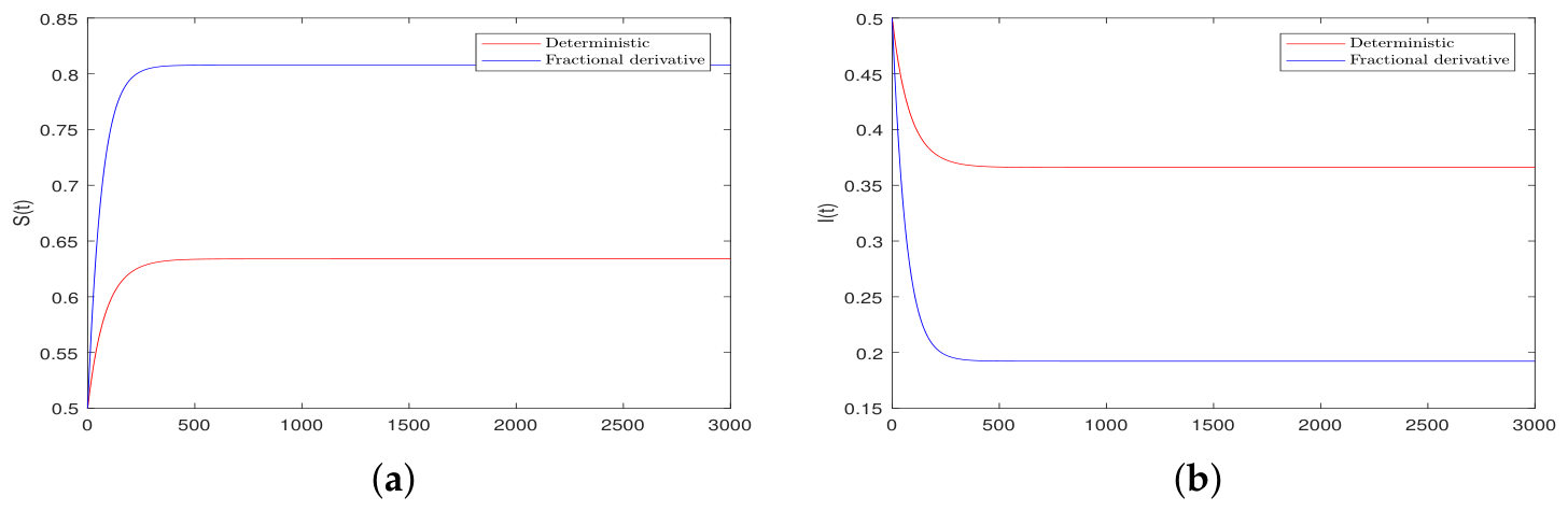
To highlight the role of the fractional memory mechanism, white-noise perturbations are not considered in this example. We only compare the trajectory differences between the classical deterministic SIS model and the fractional-order SIS model with memory effects. Figure 1 presents the trajectories of the susceptible individuals $S\left(t\right)$ and infectious individuals $I\left(t\right)$ in the two models. As shown in Figure 1, after introducing the fractional memory term, both the transient convergence process and the long-term stable levels of the system change significantly. Specifically, the fractional memory effect alters the adjustment rates of susceptible and infectious individuals and affects the long-term evolution level of $I\left(t\right)$. This indicates that historical infection states and nonlocal memory mechanisms play a non-negligible role in disease transmission, and it also provides a numerical basis for further analyzing the influence of the fractional order α on epidemic dynamics.

Figure 1. Comparison between the classical deterministic SIS model and the fractional-order SIS model without white-noise perturbations. (a) Trajectories of susceptible individuals $S\left(t\right)$; (b) trajectories of infectious individuals $I\left(t\right)$. The parameter values are $I_0=0.5$, $\Lambda =0.2$, $\beta =0.2$, $\theta =0.3$, $\gamma =0.1$, and $\alpha =0.55$, with the bilinear incidence function $f(S,I)=SI$. The white-noise intensity is set to ${\sigma }_1=0$ in this example.

Example 2.

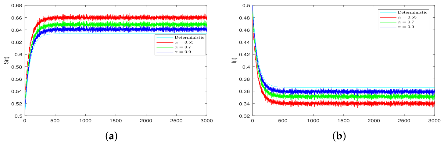
This example further investigates the influence of the fractional order α on the dynamical behavior of the model, we take $\alpha =0.5,0.7,0.9,$ while keeping the other parameters the same as those in Example 6.1. Since the fractional order α reflects the strength of the memory effect, different values of α may change the degree to which historical infection states affect the current disease transmission process. Figure 2 presents the trajectories of the susceptible individuals $S\left(t\right)$ and infectious individuals $I\left(t\right)$ in model (4) under different fractional orders.

As shown in Figure 2, the fractional order α has a significant influence on the transient evolution of the system. As α varies, the convergence rate, adjustment process, and long-term stable levels of susceptible and infectious individuals also change. In particular, the trajectories of $I\left(t\right)$ indicate that the memory intensity affects not only the short-term fluctuations and transition process of disease transmission, but also the pathway through which the infectious population evolves toward its long-term state. This demonstrates that the fractional memory mechanism is an important factor in characterizing epidemic dynamics and numerically supports the necessity of incorporating the fractional-order term into the model.

Figure 2. Trajectories of model (4) under different fractional orders $\alpha =0.5,0.7,0.9$: (a) susceptible individuals $S\left(t\right)$; (b) infectious individuals $I\left(t\right)$. The fractional orders are $\alpha =0.50,0.70,0.90$, while the remaining parameters are fixed at $I_0=0.5$, $\Lambda =0.2$, $\beta =0.2$, $\theta =0.3$, $\gamma =0.1$, and ${\sigma }_1=0.06$, with $f(S,I)=SI$.

Figure 2. Trajectories of model (4) under different fractional orders $\alpha =0.5,0.7,0.9$: (a) susceptible individuals $S\left(t\right)$; (b) infectious individuals $I\left(t\right)$. The fractional orders are $\alpha =0.50,0.70,0.90$, while the remaining parameters are fixed at $I_0=0.5$, $\Lambda =0.2$, $\beta =0.2$, $\theta =0.3$, $\gamma =0.1$, and ${\sigma }_1=0.06$, with $f(S,I)=SI$.

Example 3.

To illustrate the influence of the model parameters on the Ulam–Hyers stability estimate, we consider

$$\theta =0.3,\gamma =0.1,\alpha =0.75,T=0.1.$$

According to Theorem 3, the perturbation error satisfies

$${E|X\left(t\right)-I\left(t\right)|}^2\le M\epsilon ,M=2e^{BT},$$

where

$$B=12{(\theta +\gamma )}^{2}T+12{\beta }^2{Q}^{2}T+6{\sigma }_1^2{Q}^2+{\displaystyle \frac{6{\alpha }^2{Q}^2{T}^{2\alpha -1}}{2\alpha -1}}.$$

We consider the following three representative parameter regimes:

Regime	β	σ1	Q	M
Low sensitivity	0.10	0.03	0.30	2.0786
Moderate sensitivity	0.20	0.06	0.50	2.1543
High sensitivity	0.40	0.12	0.70	2.2947

The results show that the stability constant M increases as the transmission coefficient β, the environmental noise intensity ${\sigma }_1$, and the incidence sensitivity Q increase. Thus, smaller values of these parameters correspond to a tighter perturbation-error bound.

Epidemiologically, the low-sensitivity regime may represent reduced contact intensity, relatively stable environmental conditions, and a saturated transmission response under effective intervention measures. In contrast, the high-sensitivity regime may correspond to frequent contact, stronger environmental fluctuations, and a transmission process that is more sensitive to changes in the infectious population. In such situations, small observational or numerical errors may have a larger influence on the predicted epidemic trajectory. Among the above three regimes, we select the moderate-sensitivity case

$$\beta =0.2,{\sigma }_1=0.06,Q=0.5$$

for numerical illustration.

To examine the effect of small perturbations on the infectious trajectory, we choose the perturbed initial values

$$I_0^{\delta }=I_0+\delta ,$$

and denote by $I^{\delta }\left(t\right)$ the solution corresponding to the perturbed initial value. To eliminate the direct influence of different perturbation magnitudes on the error size, we use the normalized mean-square error

$$D_{\delta }\left(t\right)={\displaystyle \frac{E|I^{\delta }{\left(t\right)-I\left(t\right)|}^2}{{\delta }^2}}$$

to measure the deviation between the perturbed solution and the original solution.

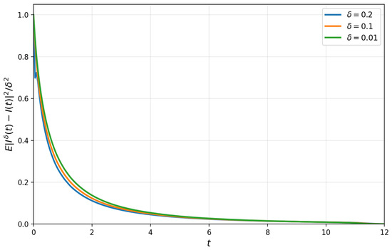
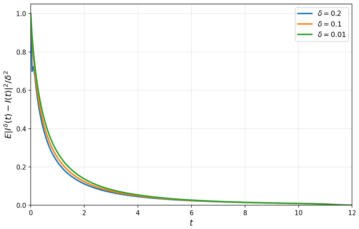
Figure 3 displays the evolution of the normalized mean-square error $D_{\delta }\left(t\right)$ under different perturbation levels. It can be seen that the curves remain bounded on $[0,T]$ and gradually decrease with time. This indicates that small perturbations in the initial value do not cause uncontrolled deviations of the infectious trajectory. Hence, the numerical result is consistent with the Ulam–Hyers stability established in Theorem 3.

Figure 3. Numerical illustration of Ulam–Hyers stability under the parameter values $\theta =0.3$, $\gamma =0.1$, $\beta =0.2$, ${\sigma }_1=0.06$, $\alpha =0.75$, $T=0.1$, and $Q=0.5$. The curves represent the normalized mean-square error $E|I^{\delta }{\left(t\right)-I\left(t\right)|}^2/{\delta }^2$ under the perturbation levels $\delta =0.2,0.1,0.01$.

Example 4.

To illustrate the averaging principle using an epidemiologically meaningful incidence function, we consider the rapidly varying seasonal incidence

$$g(t,I)=\left(1+\rho {sin}^{2}t\right){\displaystyle \frac{I(N-I)}{N(1+aI)}},0<\rho <1,a>0.$$

This function is nonnegative for

$$t\ge 0,0\le I\le N,$$

and combines periodic transmission fluctuations with a saturated incidence mechanism.

Since

$${\displaystyle \frac{1}{\pi }}{\int }_0^{\pi }{sin}^{2}tdt={\displaystyle \frac{1}{2}},$$

the corresponding averaged incidence function is

$$\begin{array}{cc}\hfill \overline{g}\left(I\right)& ={\displaystyle \frac{1}{\pi }}{\int }_0^{\pi }g(t,I)dt\hfill \\ & =\left(1+{\displaystyle \frac{\rho }{2}}\right){\displaystyle \frac{I(N-I)}{N(1+aI)}}.\hfill \end{array}$$

The original rapidly varying system is therefore given by

$$\begin{array}{cc}\hfill I^{\epsilon }\left(t\right)=& I_0+{\int }_0^t\left[\beta g\left({\displaystyle \frac{\tau }{\epsilon }},I^{\epsilon }\left(\tau \right)\right)-(\theta +\gamma )I^{\epsilon }\left(\tau \right)\right]d\tau \hfill \\ & +{\sigma }_1{\int }_0^{t}g\left({\displaystyle \frac{\tau }{\epsilon }},I^{\epsilon }\left(\tau \right)\right)dB\left(\tau \right)\hfill \\ & +\alpha {\int }_0^t{(t-\tau )}^{\alpha -1}g\left({\displaystyle \frac{\tau }{\epsilon }},I^{\epsilon }\left(\tau \right)\right)d\tau ,\hfill \end{array}$$

whereas the corresponding averaged system is

$$\begin{array}{cc}\hfill \overline{I}\left(t\right)=& I_0+{\int }_0^t\left[\beta \overline{g}\left(\overline{I}\left(\tau \right)\right)-(\theta +\gamma )\overline{I}\left(\tau \right)\right]d\tau \hfill \\ & +{\sigma }_1{\int }_0^t\overline{g}\left(\overline{I}\left(\tau \right)\right)dB\left(\tau \right)\hfill \\ & +\alpha {\int }_0^t{(t-\tau )}^{\alpha -1}\overline{g}\left(\overline{I}\left(\tau \right)\right)d\tau .\hfill \end{array}$$

In the simulation, we take

$$I_0=0.5,N=1,\beta =0.2,\theta =0.3,\gamma =0.1,$$

$${\sigma }_1=0.06,\alpha =0.75,\rho =0.6,a=0.5.$$

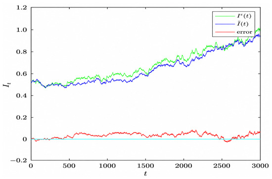
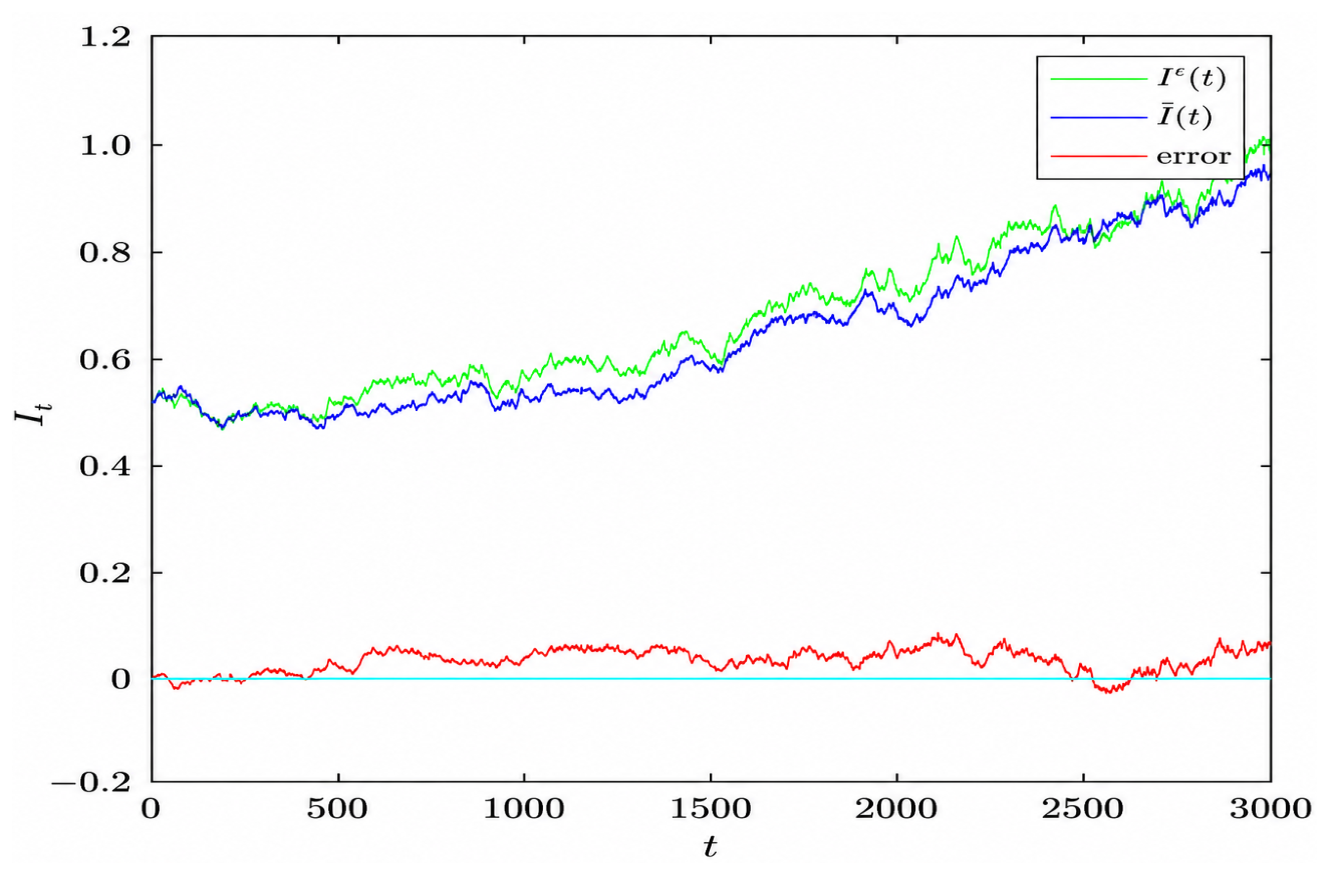
The original and averaged systems are simulated using the same Brownian increments. The numerical results show that the rapidly varying solution oscillates around the averaged trajectory and that their mean-square difference decreases as ε becomes smaller, which is consistent with the averaging principle.

Figure 4 compares the solution trajectory $I^{ϵ}\left(t\right)$ of the rapidly varying system (15) with the corresponding solution trajectory $\overline{I}\left(t\right)$ of the averaged system (16). It can be observed that the two trajectories remain close over the considered time interval, indicating that the averaged system provides an effective approximation to the dynamical behavior of the original rapidly varying system. This numerical result is consistent with the averaging principle established above, which states that, for sufficiently small ϵ, the solution $I^{ϵ}\left(t\right)$ converges to the averaged solution $\overline{I}\left(t\right)$ in the mean-square sense.

Figure 4. Comparison between the rapidly varying fractional stochastic SIS system and its averaged system for $\epsilon =0.10,0.05,0.01$. The seasonal incidence function is $g(t,I)=(1+0.6{sin}^{2}t){\displaystyle \frac{I(1-I)}{1+0.5I}},$ and the averaged incidence is $\overline{g}\left(I\right)=1.3{\displaystyle \frac{I(1-I)}{1+0.5I}}.$ The remaining parameters are $I_0=0.5$, $\beta =0.2$, $\theta =0.3$, $\gamma =0.1$, ${\sigma }_1=0.06$, and $\alpha =0.75$. The same Brownian increments are used for all comparisons.

Example 5.

To numerically illustrate the almost-sure extinction result in Theorem 2, we consider the standard incidence function $f(S,I)={\displaystyle \frac{SI}{N}}.$

We choose

$$N=1,I_0=0.5,\beta =0.2,\theta =0.3,\gamma =0.1,$$

$${\sigma }_1=0.06,\alpha =0.75.$$

Then,

$${\tilde{R}}_0={\displaystyle \frac{\beta g^{\prime }\left(0\right)}{\theta +\gamma }}={\displaystyle \frac{0.2}{0.3+0.1}}=0.5<1.$$

Moreover,

$$g^{\prime }\left(0\right)=1<{\displaystyle \frac{\beta }{{\sigma }_1^2}}.$$

Therefore, the sufficient conditions of Theorem 2 are satisfied.

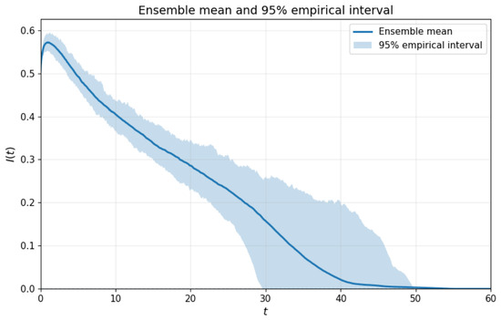
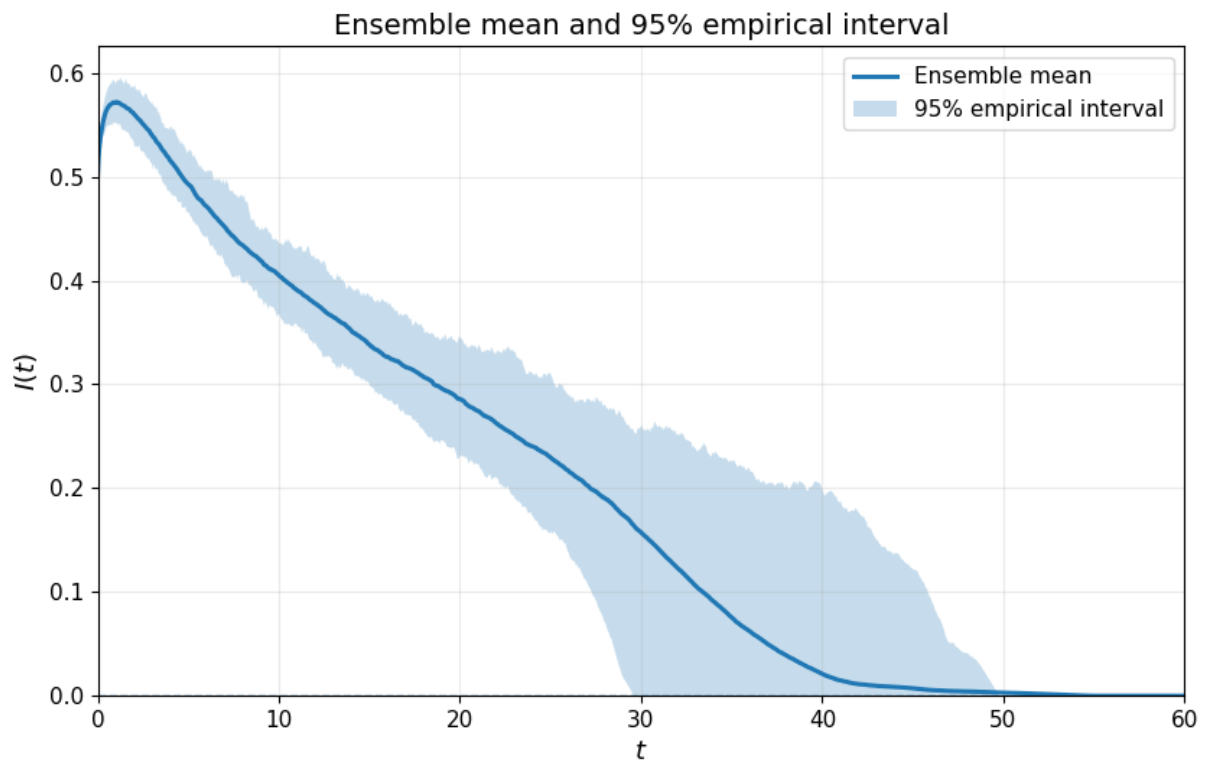
The simulated sample paths of $I\left(t\right)$ decrease toward zero, and the ensemble mean also converges to zero as time increases. These results provide a direct numerical illustration of the almost-sure disease extinction predicted by Theorem 2.

Figure 5 presents the ensemble mean and the 95% empirical interval of the infectious population obtained from 100 independent simulations. After a short initial fluctuation, the ensemble mean exhibits a clear downward trend and gradually approaches zero. Meanwhile, the empirical interval also contracts toward the disease-free state as time increases. This numerical result is consistent with the almost-sure extinction conclusion of Theorem 2 under the condition ${\tilde{R}}_0<1$.

Figure 5. Numerical illustration of disease extinction under ${\tilde{R}}_0<1$. The standard incidence function $g\left(I\right)=I(1-I)$ is considered with $I_0=0.5$, $N=1$, $\beta =0.2$, $\theta =0.3$, $\gamma =0.1$, ${\sigma }_1=0.06$, and $\alpha =0.75$, for which ${\tilde{R}}_0=0.5<1$. The solid curve represents the ensemble mean, and the shaded region represents the 95% empirical interval obtained from 100 independent simulations. The ensemble mean and empirical interval gradually approach zero, illustrating convergence toward the disease-free state.

7. Empirical Analysis Based on SDEPINN

To further examine the applicability of the SIS-type epidemic dynamics framework proposed in this study to real-world epidemiological data, we conduct an empirical analysis using monthly reported influenza cases from the Xinjiang Uygur Autonomous Region. The data are obtained from the statutory infectious disease epidemic bulletins officially released by the Health Commission of Xinjiang Uygur Autonomous Region. The sample period spans from January 2020 to February 2026, covering a total of 74 monthly observations. This monthly dataset objectively characterizes the temporal evolution of influenza activity intensity in Xinjiang.

7.1. Relationship Between the Theoretical and Empirical Models

The theoretical model developed in the preceding sections contains a general nonlinear incidence function, a Brownian perturbation, and a fractional memory term. Since the available observations consist of monthly aggregated case counts, the underlying continuous-time Brownian increments cannot be separately identified from the data. Therefore, a reliable pathwise reconstruction of the stochastic forcing is not feasible. For empirical fitting, we consequently omit the unobserved Brownian integral and consider a reduced deterministic fractional integral model as a practically identifiable approximation of the theoretical stochastic model.

For the empirical analysis, the total population is normalized as $N=1,$ and the standard bilinear incidence function $f(S,I)=SI$ is adopted. Since $S=1-I$, it follows that $g\left(I\right)=f(1-I,I)=I(1-I).$ Moreover, we define $\delta =\theta +\gamma$ as the total removal rate of infectious individuals. After omitting the unobserved Brownian integral, the reduced empirical model is written as

$$\begin{array}{cc}\hfill I\left(t\right)=& I_0+{\int }_0^t\left[\beta \left(s\right)I\left(s\right)(1-I(s\left)\right)-\delta I\left(s\right)\right]ds\hfill \\ \hfill & +\alpha {\int }_0^t{(t-s)}^{\alpha -1}I\left(s\right)(1-I\left(s\right))ds.\hfill \end{array}$$

(23)

The neural-network framework below uses model (23) as its physical constraint. The reduced model preserves the nonlinear incidence and fractional memory structures of the theoretical model, while the Brownian trajectory is not reconstructed pathwise. This simplification is introduced for practical identifiability under monthly aggregated observations and does not diminish the role of stochasticity in the theoretical analysis. Thus, the stochastic model provides the mathematical and mechanistic foundation, whereas the reduced deterministic fractional model serves as the empirically identifiable constraint for data fitting.

7.2. Seasonally Enhanced SDEPINN Algorithm

Let $y_t$ denote the number of reported influenza cases in Xinjiang in month t, and define the log-transformed case count as $q_t=log(1+y_t).$ To make the empirical state consistent with the normalized SIS model, the log-transformed case counts are rescaled to the interval $[0,1]$:

$$I_t^{\mathrm{obs}}={\displaystyle \frac{q_t-q_{min}}{q_{max}-q_{min}}},$$

(24)

where

$$q_{min}=\underset{1\le j\le n}{min}{q}_j,q_{max}=\underset{1\le j\le n}{max}{q}_j.$$

This transformation effectively compresses the scale effect of extreme peaks, enabling the model to maintain good fitting performance during both low-incidence and high-incidence periods.

The fitting framework adopts a dual-branch multilayer perceptron architecture. The first branch predicts the normalized infection state:

$$I_{\mathbf{\Theta }}\left(t\right)=sigmoid\left(f_{\mathit{\theta }}\left({\mathbf{x}}_t\right)\right).$$

(25)

The second branch network, denoted by $g_{\varphi }(·)$, is used to estimate the time-varying transmission intensity. To ensure the non-negativity of the transmission intensity, the softplus function is applied:

$${\beta }_{\mathbf{\Theta }}\left(t\right)=softplus\left(g_{\mathit{\varphi }}\left({\mathbf{x}}_t\right)\right).$$

The total removal rate is constrained to be positive by

$$\delta =softplus\left({\eta }_{\delta }\right),$$

(26)

where ${\eta }_{\delta }$ is a trainable scalar parameter.

Let $I_{\mathbf{\Theta }}\left(t\right)$ and ${\beta }_{\mathbf{\Theta }}\left(t\right)$ denote the infection state and the time-varying transmission rate predicted by the neural network, respectively. Based on model (23), the physics-informed integral residual is defined as

$$\begin{array}{cc}\hfill {\mathcal{R}}_{\mathbf{\Theta }}\left(t\right)=& I_{\mathbf{\Theta }}\left(t\right)-I_0\hfill \\ \hfill & -{\int }_0^t\left[{\beta }_{\mathbf{\Theta }}\left(s\right)I_{\mathbf{\Theta }}\left(s\right)\left(1-I_{\mathbf{\Theta }}\left(s\right)\right)-\delta I_{\mathbf{\Theta }}\left(s\right)\right]ds\hfill \\ \hfill & -\alpha {\int }_0^t{(t-s)}^{\alpha -1}{I}_{\mathbf{\Theta }}\left(s\right)\left(1-I_{\mathbf{\Theta }}\left(s\right)\right)ds.\hfill \end{array}$$

(27)

This residual measures the difference between the neural-network output and the right-hand side of the reduced integral model.

The physics-informed loss is defined by minimizing the integral residual at the collocation points:

$${\mathcal{L}}_{\mathrm{phy}}={\displaystyle \frac{1}{N_r}}{\displaystyle \sum _{j=1}^{N_r}}{\left|{\mathcal{R}}_{\mathbf{\Theta }}\left(t_j\right)\right|}^2.$$

(28)

The integral residual provides a mechanistic constraint consistent with the reduced SIS model, while the relatively small physics-loss weight maintains sufficient flexibility to fit abrupt variations in the monthly influenza observations.

$${\mathcal{L}}_{\mathrm{data}}={\displaystyle \frac{1}{n}}{\displaystyle \sum _{j=1}^n}{w}_j{\left[I_{\mathbf{\Theta }}\left(t_j\right)-I_j^{\mathrm{obs}}\right]}^2,$$

(29)

where $w_j=1+\rho {\left({\displaystyle \frac{y_j}{{max}_{1\le \ell \le n}{y}_{\ell }}}\right)}^p.$ When $y_t$ is large, the corresponding weight $w_t$ increases, thereby encouraging the model to pay greater attention to high-incidence months during training. In this study, we set $\rho =4.0$ and $p=1.5$.

The smoothness loss for the time-varying transmission rate is defined as

$${\mathcal{L}}_{\mathrm{smooth}}={\displaystyle \frac{1}{n-1}}{\displaystyle \sum _{j=1}^{n-1}}{\left[{\beta }_{\mathbf{\Theta }}\left(t_{j+1}\right)-{\beta }_{\mathbf{\Theta }}\left(t_j\right)\right]}^2.$$

(30)

The initial-condition loss is defined as

$${\mathcal{L}}_{\mathrm{init}}={\left|I_{\mathbf{\Theta }}\left(0\right)-I_0\right|}^2.$$

(31)

Therefore, the total loss function is defined as

$$\mathcal{L}={\lambda }_d{\mathcal{L}}_{data}+{\lambda }_r{\mathcal{L}}_{phy}+{\lambda }_s{\mathcal{L}}_{smooth}+{\lambda }_0{\mathcal{L}}_{init},$$

(32)

where ${\mathcal{L}}_{smooth}$ denotes the smoothness constraint on the transmission intensity ${\beta }_t$, and ${\mathcal{L}}_{init}$ denotes the initial-condition constraint. The weights are set as

$${\lambda }_d=1.0,{\lambda }_r=0.01,{\lambda }_s=0.003,{\lambda }_0=0.05.$$

(33)

This setting indicates that data fitting is the primary objective of the model, while the dynamical residual and smoothness constraints mainly serve as weak regularization terms.

To evaluate residual (27), define

$$F_{\mathbf{\Theta }}\left(s\right)={\beta }_{\mathbf{\Theta }}\left(s\right)I_{\mathbf{\Theta }}\left(s\right)\left(1-I_{\mathbf{\Theta }}\left(s\right)\right)-\delta I_{\mathbf{\Theta }}\left(s\right)$$

and

$$G_{\mathbf{\Theta }}\left(s\right)=I_{\mathbf{\Theta }}\left(s\right)\left(1-I_{\mathbf{\Theta }}\left(s\right)\right).$$

For the ordinary integral, the trapezoidal rule is used:

$${\int }_0^{t_n}{F}_{\mathbf{\Theta }}\left(s\right)ds\approx {\displaystyle \sum _{j=0}^{n-1}}{\displaystyle \frac{F_{\mathbf{\Theta }}\left(t_j\right)+F_{\mathbf{\Theta }}\left(t_{j+1}\right)}{2}}\Delta t_j,$$

(34)

where $\Delta t_j=t_{j+1}-t_j$. For the fractional memory term, we use the product-integration approximation

$$\alpha {\int }_0^{t_n}{(t_n-s)}^{\alpha -1}{G}_{\mathbf{\Theta }}\left(s\right)ds\approx {\displaystyle \sum _{j=0}^{n-1}}{\omega }_{n,j}^{\left(\alpha \right)}{G}_{\mathbf{\Theta }}\left(t_j\right),$$

(35)

where ${\omega }_{n,j}^{\left(\alpha \right)}={(t_n-t_j)}^{\alpha }-{(t_n-t_{j+1})}^{\alpha }.$ This discretization preserves the power-law memory weights and avoids direct evaluation of the weakly singular kernel at $s=t_n$.

In terms of network architecture, the main fitting network consists of three hidden layers, each containing 96 neurons, with the Tanh activation function and a dropout rate of 0.03. The transmission-rate network for ${\beta }_{\mathbf{\Theta }}$ consists of two hidden layers, each containing 48 neurons, and applies the softplus function to ensure positive outputs. The model parameters are initialized using the Xavier initialization method.

For model training, the AdamW optimizer is employed, with the learning rate set to $8\times {10}^{-4}$ and the weight decay coefficient set to $1\times {10}^{-5}$. The maximum number of training epochs is 5000, and the early-stopping patience is set to 700. Since the data are monthly time-series observations with a relatively limited sample size, full-batch training is adopted.

To reduce the sensitivity of a single neural network to random initialization and local optima, this study adopts a randomized ensemble training strategy. Specifically, small random perturbations are added to the standardized case series, and the loss-function weights are also randomly perturbed. A total of $K=16$ sub-models are trained repeatedly. For the k-th sub-model, let ${\widehat{I}}_t^{\left(k\right)}=I_{{\mathbf{\Theta }}^{\left(k\right)}}\left(t\right)$ denote the predicted normalized infection state at time t. It is transformed back to the original case-count scale by

$${\widehat{y}}_t^{\left(k\right)}=exp\left[q_{min}+{\widehat{I}}_t^{\left(k\right)}\left(q_{max}-q_{min}\right)\right]-1.$$

(36)

The final model output is obtained by averaging the fitted values of the 16 sub-models:

$${\overline{y}}_t={\displaystyle \frac{1}{K}}{\displaystyle \sum _{k=1}^K}{\widehat{y}}_t^{\left(k\right)}.$$

(37)

Meanwhile, the 2.5% and 97.5% quantiles of the fitted results from all sub-models are used to construct the 95% ensemble uncertainty interval. This interval reflects the uncertainty of the model in fitting the historical case series and should not be interpreted as a strict Bayesian credible interval or a future prediction interval.

7.3. Model Evaluation Metrics

To evaluate the fitting performance of the proposed model for the influenza case series in Xinjiang, this study employs five commonly used evaluation metrics: mean absolute error (MAE), root mean square error (RMSE), mean absolute percentage error (MAPE), symmetric mean absolute percentage error (SMAPE), and the coefficient of determination $\left(R^2\right)$. These metrics are defined as follows:

$$\begin{array}{cccc}\hfill MAE& ={\displaystyle \frac{1}{n}}{\displaystyle \sum _{t=1}^n}|y_t-{\widehat{y}}_t|,\hfill & \hfill RMSE& =\sqrt{{\displaystyle \frac{1}{n}}\sum _{t=1}^n{(y_t-{\widehat{y}}_t)}^2},\hfill \\ \hfill MAPE& ={\displaystyle \frac{100\%}{n}}{\displaystyle \sum _{t=1}^n}\left|{\displaystyle \frac{y_t-{\widehat{y}}_t}{max(y_t,1)}}\right|,\hfill & \hfill SMAPE& ={\displaystyle \frac{100\%}{n}}{\displaystyle \sum _{t=1}^n}{\displaystyle \frac{2|y_t-{\widehat{y}}_t|}{max\left(\right|y_t|+|{\widehat{y}}_t|,1)}}.\hfill \end{array}$$

Here, MAE and RMSE are used to measure the absolute errors on the original case-count scale, while MAPE and SMAPE are used to measure relative errors. The coefficient of determination, $R^2$, is used to evaluate the explanatory ability of the model with respect to fluctuations in the case series.

7.4. Empirical Results Analysis

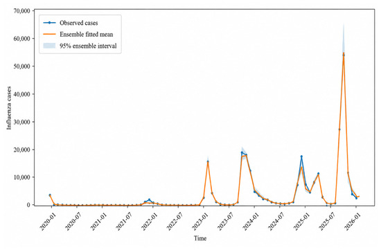
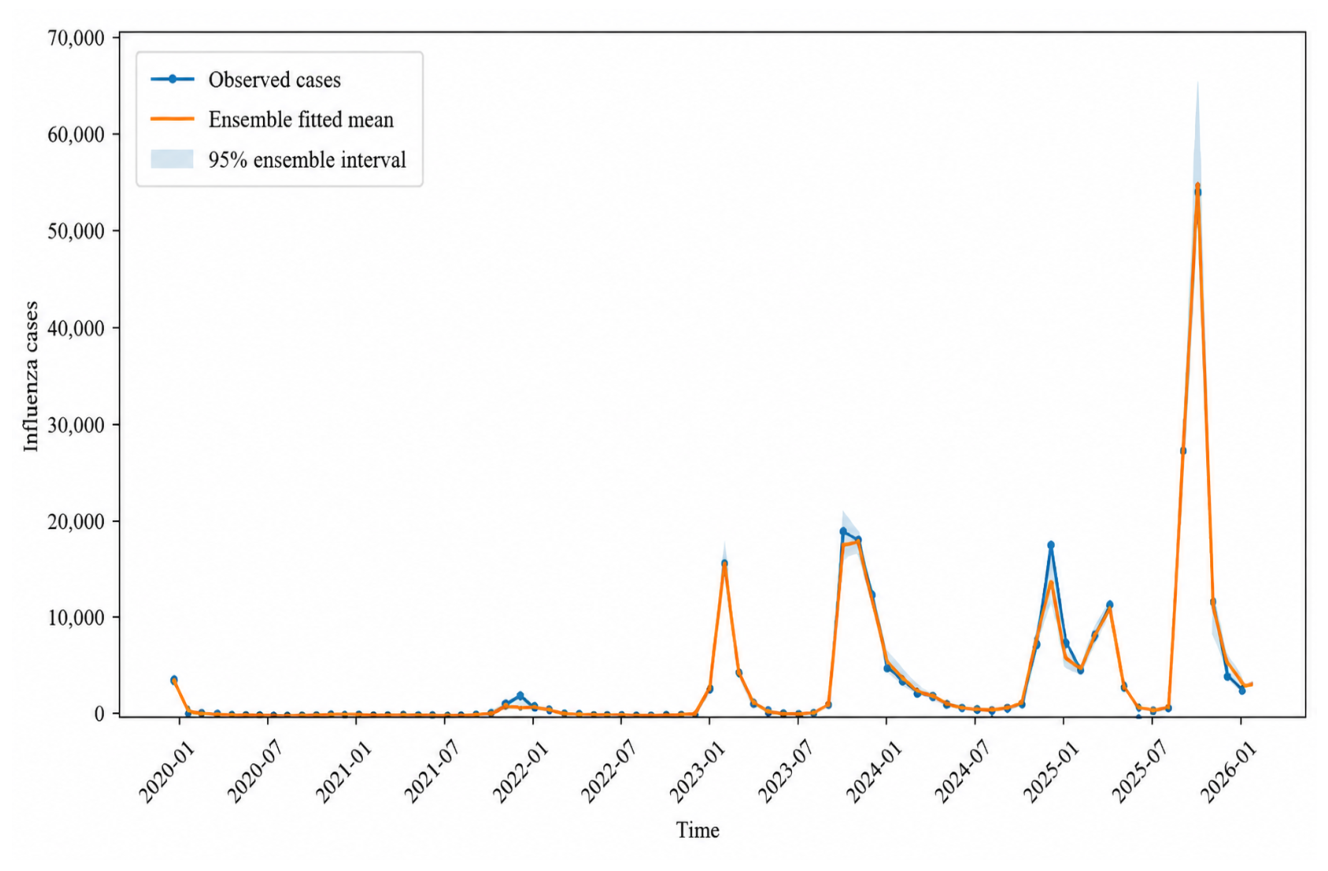
Figure 6 presents the fitting results of monthly reported influenza cases in Xinjiang obtained using the seasonally SDEPINN algorithm. The results show that the algorithm can effectively characterize the main temporal variation features of influenza cases in Xinjiang. During low-incidence periods, the fitted curve remains at a relatively low level without producing obvious artificial peaks. During high-incidence periods, the algorithm can capture the timing and magnitude changes of the major case peaks occurring in early 2023, from autumn and winter 2023 to early 2024, in early 2025, and in autumn and winter 2025. In particular, during periods of rapid increase and rapid decline in case numbers, the fitted curve remains highly consistent with the observed sequence.

Figure 6. Fitting results of monthly reported influenza cases in Xinjiang using the seasonal SDEPINN. The blue line with markers represents the observed monthly reported influenza cases, the orange line denotes the ensemble fitted mean produced by the seasonally enhanced SDEPINN, and the light-blue shaded area indicates the 95% ensemble uncertainty interval constructed from the 2.5% and 97.5% quantiles of the fitted results from 16 randomized sub-models.

From the perspective of the model mechanism, the favorable fitting performance mainly arises from three aspects. First, the annual and semiannual sine-cosine periodic terms, the cold-season indicator, and the monthly dummy variables jointly enhance the model’s ability to represent the seasonal rhythm of influenza, enabling it to identify differences in influenza activity intensity across different months. Second, the transformation $log(1+y_t)$ compresses the scale effect of extreme peaks, reduces the impact of large fluctuations in raw case counts on training stability, and enables the model to balance fitting accuracy between low-incidence and high-incidence periods. Third, the peak-weighted loss function increases the contribution of high-incidence months during training, thereby reducing the model’s systematic underestimation of outbreak peaks.

Table 1 presents the in-sample fitting evaluation results of the model. As shown in Table 1, the model achieves an $R^2$ value of 0.9951, indicating that the fitted values can explain most of the temporal fluctuations in the reported influenza cases in Xinjiang. The MAE and RMSE are 212.0771 and 545.2049, respectively, suggesting that the average fitting errors on the original case-count scale are relatively small. The MAPE and SMAPE are 10.6737% and 9.7341%, respectively, indicating that the model also exhibits good fitting performance in terms of relative errors.

Table 1. Fitting performance of the proposed model for influenza cases in Xinjiang.

Metric	MAE	RMSE	MAPE (%)	SMAPE (%)	${\mathit{R}}^2$
Value	212.0771	545.2049	10.6737	9.7341	0.9951

8. Conclusions

Considering that historical infection data has impacted the future evolution of the epidemic, fractional differentiation is introduced into the conventional stochastic epidemic model in this paper. Firstly, based on the properties of fractional differential equations, a random process was constructed, which transforms the proof of the existence and uniqueness of model solutions into that of the existence and uniqueness of sequence limits. Secondly, under certain conditions, the extinction of the infected individuals and the Ulam–Hyers stability of the model are obtained using Hölder’s inequality, the Burkholder–Davis–Gundy inequality, Gronwall inequality, and Itô’s isometry. Finally, we demonstrated that solutions of the averaged stochastic model can approximate the solutions of the model in the sense of mean square. In other words, the average principle provided a convenient and feasible method for studying properties based on the related averaged equations.

In addition, this paper constructs a seasonally enhanced SDEPINN framework. This framework integrates fractional stochastic dynamical residuals with seasonal features, and adopts a peak-weighted loss function and an ensemble training strategy. Empirical results based on influenza data from Xinjiang show that the proposed framework can effectively capture seasonal fluctuations and outbreak peaks of the epidemic, while providing an ensemble-based empirical uncertainty band.

It is worth noting that model (4) is transformed into model (8) under certain specific conditions, which results in a limited applicability of the model. On the other hand, multi-time scale differential remains a niche area of study, with most research focusing on Riemann–Liouville and Caputo fractional differential. Therefore, it is our further work to extend these conclusions to multidimensional Caputo fractional stochastic epidemic models.

References

- Biswas, M.H.A.; Paiva, L.T.; de Pinho, M.D.R. A SEIR model for control of infectious diseases with constraints. Math. Biosci. Eng. 2014, 11, 761–784. [Google Scholar] [CrossRef] [Scilit]
- Kabir, K.A.; Kuga, K.; Tanimoto, J. Analysis of SIR epidemic model with information spreading of awareness. Chaos Solitons Fractals 2019, 119, 118–125. [Google Scholar] [CrossRef] [Scilit]
- Li, H.; Peng, R. Dynamics and asymptotic profiles of endemic equilibrium for SIS epidemic patch models. J. Math. Biol. 2019, 79, 1279–1317. [Google Scholar] [CrossRef] [Scilit] [PubMed]
- Wu, Z.; Cai, Y.; Wang, Z.; Wang, W. Global stability of a fractional order SIS epidemic model. J. Differ. Equ. 2023, 352, 221–248. [Google Scholar] [CrossRef] [Scilit]
- Tang, J.; Yao, Y.; Xie, M.; Feng, M. SIS Epidemic Modelling on Homogeneous Networked System: General Recovering Process and Mean-Field Perspective. Appl. Math. Model. 2025, 146, 116188. [Google Scholar] [CrossRef] [Scilit]
- Din, A.; Khan, A.; Baleanu, D. Stationary distribution and extinction of stochastic coronavirus (COVID-19) epidemic model. Chaos Solitons Fractals 2020, 139, 110036. [Google Scholar] [CrossRef] [Scilit] [PubMed]
- Din, A.; Khan, T.; Li, Y.; Tahir, H.; Khan, A.; Khan, W.A. Mathematical analysis of dengue stochastic epidemic model. Results Phys. 2021, 20, 103719. [Google Scholar] [CrossRef] [Scilit]
- Din, A.; Li, Y.; Yusuf, A. Delayed hepatitis B epidemic model with stochastic analysis. Chaos Solitons Fractals 2021, 146, 110839. [Google Scholar] [CrossRef] [Scilit]
- Zhang, G.; Li, Z.; Din, A. A stochastic SIQR epidemic model with Lévy jumps and three-time delays. Appl. Math. Comput. 2022, 431, 127329. [Google Scholar] [CrossRef] [Scilit] [PubMed]
- Midhun, T.; Murugesan, K. A study of stochastically perturbed epidemic model of HPV infection and cervical cancer in Indian female population. Math. Comput. Simul. 2025, 228, 431–465. [Google Scholar] [CrossRef] [Scilit]
- Cai, Y.; Kang, Y.; Banerjee, M.; Wang, W. A stochastic SIRS epidemic model with infectious force under intervention strategies. J. Differ. Equ. 2015, 259, 7463–7502. [Google Scholar] [CrossRef] [Scilit]
- Xu, C.; Yuan, S. An analogue of break-even concentration in a simple stochastic chemostat model. Appl. Math. Lett. 2015, 48, 62–68. [Google Scholar] [CrossRef] [Scilit]
- Teng, Z.; Wang, L. Persistence and extinction for a class of stochastic SIS epidemic models with nonlinear incidence rate. Phys. A Stat. Mech. Its Appl. 2016, 451, 507–518. [Google Scholar] [CrossRef] [Scilit]
- Zhu, C. Critical result on the threshold of a stochastic SIS model with saturated incidence rate. Phys. A Stat. Mech. Its Appl. 2019, 523, 426–437. [Google Scholar] [CrossRef] [Scilit]
- Dineshkumar, C.; Udhayakumar, R.; Vijayakumar, V.; Nisar, K.S.; Shukla, A. A note concerning to approximate controllability of Atangana-Baleanu fractional neutral stochastic systems with infinite delay. Chaos Solitons Fractals 2022, 157, 111916. [Google Scholar] [CrossRef] [Scilit]
- Broucke, F.; Oparnica, L. Micro-local and qualitative analysis of the fractional Zener wave equation. J. Differ. Equ. 2022, 321, 217–257. [Google Scholar] [CrossRef] [Scilit]
- Luo, D.; Tian, M.; Zhu, Q. Some results on finite-time stability of stochastic fractional-order delay differential equations. Chaos Solitons Fractals 2022, 158, 111996. [Google Scholar] [CrossRef] [Scilit]
- Liaqat, M.I.; Riaz, M.B.; Akgül, A. Theoretical Analysis of Time Fractal Fractional Pantograph Stochastic Differential Equations. Partial Differ. Equ. Appl. Math. 2025, 15, 101258. [Google Scholar] [CrossRef] [Scilit]
- El-Borai, M.M.; El-Nadi, K.E.S.; Fouad, H.A. On some fractional stochastic delay differential equations. Comput. Math. Appl. 2010, 59, 1165–1170. [Google Scholar] [CrossRef] [Scilit]
- Sakthivel, R.; Revathi, P.; Ren, Y. Existence of solutions for nonlinear fractional stochastic differential equations. Nonlinear Anal. Theory Methods Appl. 2013, 81, 70–86. [Google Scholar] [CrossRef] [Scilit]
- Wang, Y.; Xu, J.; Kloeden, P.E. Asymptotic behavior of stochastic lattice systems with a Caputo fractional time derivative. Nonlinear Anal. Theory Methods Appl. 2016, 135, 205–222. [Google Scholar] [CrossRef] [Scilit]
- Son, D.T.; Huong, P.T.; Kloeden, P.E.; Tuan, H.T. Asymptotic separation between solutions of Caputo fractional stochastic differential equations. Stoch. Anal. Appl. 2018, 36, 654–664. [Google Scholar] [CrossRef] [Scilit]
- Xu, J.; Zhang, Z.; Caraballo, T. Mild solutions to time fractional stochastic 2D-Stokes equations with bounded and unbounded delay. J. Dyn. Differ. Equ. 2022, 34, 583–603. [Google Scholar] [CrossRef] [Scilit]
- Lv, T.; Yang, M. A Study Concerning to the Existence and Averaging Principle for ψ-Hilfer Fractional Stochastic Evolution Equations. Math. Methods Appl. Sci. 2025, 48, 15773–15783. [Google Scholar] [CrossRef] [Scilit]
- Wang, W.; Cheng, S.; Guo, Z.; Yan, X. A note on the continuity for Caputo fractional stochastic differential equations. Chaos Interdiscip. J. Nonlinear Sci. 2020, 30, 073106. [Google Scholar] [CrossRef] [Scilit] [PubMed]
- Khasminskij, R. On the principle of averaging the Itov’s stochastic differential equations. Kybernetika 1968, 4, 260–279. [Google Scholar]
- Gao, P. Averaging principle for stochastic Korteweg-de Vries equation. J. Differ. Equ. 2019, 267, 6872–6909. [Google Scholar] [CrossRef] [Scilit]
- Xu, W.; Duan, J.; Xu, W. An averaging principle for fractional stochastic differential equations with Lévy noise. Chaos Interdiscip. J. Nonlinear Sci. 2020, 30, 083126. [Google Scholar] [CrossRef] [Scilit] [PubMed]
- Xu, Y.; Duan, J.; Xu, W. An averaging principle for stochastic dynamical systems with Lévy noise. Phys. D Nonlinear Phenom. 2011, 240, 1395–1401. [Google Scholar] [CrossRef] [Scilit]
- Guo, Z.; Lv, G.; Wei, J. Averaging principle for stochastic differential equations under a weak condition. Chaos Interdiscip. J. Nonlinear Sci. 2020, 30, 123139. [Google Scholar] [CrossRef] [Scilit] [PubMed]
- Guo, Z.; Hu, J.; Yuan, C. Averaging principle for a type of Caputo fractional stochastic differential equations. Chaos Interdiscip. J. Nonlinear Sci. 2021, 31, 053123. [Google Scholar] [CrossRef] [Scilit] [PubMed]
- Liu, J.; Zhang, H.; Wang, J.; Jin, C.; Li, J.; Xu, W. A Note on Averaging Principles for Fractional Stochastic Differential Equations. Fractal Fract. 2024, 8, 216. [Google Scholar] [CrossRef] [Scilit]
- Shen, G.; Sakthivel, R.; Ren, Y.; Li, M. Controllability and stability of fractional stochastic functional systems driven by Rosenblatt process. Collect. Math. 2020, 71, 63–82. [Google Scholar] [CrossRef] [Scilit]
- Liu, K.; Wang, J.; Zhou, Y.; O’Regan, D. Hyers–Ulam stability and existence of solutions for fractional differential equations with Mittag–Leffler kernel. Chaos Solitons Fractals 2020, 132, 109534. [Google Scholar] [CrossRef] [Scilit]
- Yang, J.W.; Yu, Z.G.; Shi, L. A new fractional-order anomalous epidemic model on complex networks based on continuous-time random walk and its dynamics. Chaos Interdiscip. J. Nonlinear Sci. 2025, 35, 113112. [Google Scholar] [CrossRef] [Scilit] [PubMed]
- Glöckle, W.G.; Nonnenmacher, T.F. A fractional calculus approach to self-similar protein dynamics. Biophys. J. 1995, 68, 46–53. [Google Scholar] [CrossRef] [Scilit] [PubMed]
- Moualkia, S. Mathematical analysis of new variant Omicron model driven by Lévy noise and with variable-order fractional derivatives. Chaos Solitons Fractals 2023, 167, 113030. [Google Scholar] [CrossRef] [Scilit]
- Jumarie, G. New stochastic fractional models for Malthusian growth, the Poissonian birth process and optimal management of populations. Math. Comput. Model. 2006, 44, 231–254. [Google Scholar] [CrossRef] [Scilit]
- Pedjeu, J.C.; Ladde, G.S. Stochastic fractional differential equations: Modeling, method and analysis. Chaos Solitons Fractals 2012, 45, 279–293. [Google Scholar] [CrossRef] [Scilit]
- Han, S.; Stelz, L.; Stoecker, H.; Wang, L.; Zhou, K. Approaching Epidemiological Dynamics of COVID-19 with Physics-Informed Neural Networks. J. Frankl. Inst. 2024, 361, 106671. [Google Scholar] [CrossRef] [Scilit]
- Li, R.; Song, Y.; Qu, H.; Li, M.; Jiang, G.P. A Data-Driven Epidemic Model with Human Mobility and Vaccination Protection for COVID-19 Prediction. J. Biomed. Inform. 2024, 149, 104571. [Google Scholar] [CrossRef] [Scilit] [PubMed]
- Diao, H.; Wen, G.; Xu, S.; Hu, W.; Nian, F. Physics-Informed GNN Epidemic Forecasting via Double-Layer Dynamic Model. IEEE Trans. Comput. Soc. Syst. 2025, 12, 4547–4560. [Google Scholar] [CrossRef] [Scilit]
- Rahman, J.U.; Arshad, M.; Mustafa, N. A Boundary-Aware PINN Framework for Monkeypox Transmission Dynamics Using Chebyshev-Distributed Collocation. Int. J. Appl. Comput. Math. 2025, 11, 251. [Google Scholar] [CrossRef] [Scilit]
- Gupta, A.; Chouhan, U. Solving Stiff Syndemic Dynamics: A Climate-Integrated Physics-Informed Neural Network Reveals Hidden Malaria-Dengue Coinfections. Chaos Solitons Fractals 2026, 209, 118413. [Google Scholar] [CrossRef] [Scilit]
- Ali, A.; Sun, M.; Ali, M.R. Data Analysis of Dynamical System for the Optimization of Disease Dynamics through Neural Networks Paradigm. Chaos Solitons Fractals 2025, 196, 116284. [Google Scholar] [CrossRef] [Scilit]
- Xie, L.; Yang, J.; Li, Z. Dynamic Properties of an SARS-CoV-2 Epidemic Model via Stochastic PINNs. Infect. Dis. Model. 2026, 11, 1180–1205. [Google Scholar] [CrossRef] [Scilit] [PubMed]
- Sahoo, P.; Riedel, T. Mean Value Theorems and Functional Equations; World Scientific: Singapore, 1998. [Google Scholar]
- Abouagwa, M.; Li, J. Carathéodory approximations and stability of solutions to non-Lipschitz stochastic fractional differential equations of Itô–Doob type. Appl. Math. Comput. 2018, 329, 143–153. [Google Scholar] [CrossRef] [Scilit]
- Guo, Z.; Hu, J.; Wang, W. Carathéodory’s approximation for a type of Caputo fractional stochastic differential equations. Adv. Differ. Equ. 2020, 2020, 636. [Google Scholar] [CrossRef] [Scilit]
Disclaimer/Publisher’s Note: The statements, opinions and data contained in all publications are solely those of the individual author(s) and contributor(s) and not of MDPI and/or the editor(s). MDPI and/or the editor(s) disclaim responsibility for any injury to people or property resulting from any ideas, methods, instructions or products referred to in the content. |
© 2026 by the authors. Licensee MDPI, Basel, Switzerland. This article is an open access article distributed under the terms and conditions of the Creative Commons Attribution (CC BY) license.