PID Control of α-Order Systems in Fractal Time

Abstract

This paper presents a novel proportional–integral–derivative (PID) control framework for first $\alpha$-order systems evolving in fractal time. The main contribution is the extension of classical control theory to systems exhibiting anomalous temporal scaling by employing local fractal derivatives. In contrast to fractional-order PID (FOPID) approaches, which primarily model memory effects, the proposed fractal PID framework captures time-scaling behavior arising in non-smooth environments, such as viscoelastic friction and irregular contact surfaces. The closed-loop dynamics are formulated as a second $\alpha$-order fractal differential equation, from which a characteristic equation is derived to establish conditions for asymptotic stability. It is shown that, for a constant reference input and positive controller gains, the tracking error converges to zero as $t\to \infty$. In addition, a quantitative performance analysis demonstrates that the fractal-order $\alpha$ governs temporal stretching: smaller values of $\alpha$ lead to increased rise and settling times and reduced oscillation frequency. The effectiveness of the proposed approach is illustrated through applications to a thermal system with fractal heat input and robotic actuators operating in irregular environments. These results highlight the potential of fractal-time control as a systematic framework for modeling and controlling dynamical systems with non-integer temporal structure.

1. Introduction

Fractal geometry provides a powerful framework for analyzing irregular and self-similar patterns in nature, such as vascular networks, coastlines, and clouds. These structures are characterized by fractional dimensions and scale invariance, with their complexity measured by the fractal dimension, which captures how detail evolves across different scales [1,2]. Fractal time has been explored in various contexts, particularly in physics and complex systems [3,4,5,6,7]. To study such systems, fractal calculus has been developed as an extension of classical calculus, enabling the modeling of dynamics on fractal sets and systems with non-integer dimensional time and space [8,9]. Recent advances, including non-local formulations and generalized integral definitions, have further strengthened this framework and enabled the description of systems exhibiting power-law scaling and self-similar behavior [7,10].

The problem of stabilizing a first-order plant with dead-time using a proportional–integral–derivative (PID) controller has been widely studied [11]. The selection of the filter has been recognized as an important factor in internal model control (IMC)-based controller design. For minimum-phase delay-free plants, an IMC-based controller has been obtained by augmenting a filter [12]. A set of tuning rules for standard (integer-order) PID and fractional-order PID controllers has been presented. In particular, for processes modeled as first-order-plus-dead-time systems, these rules are often derived to minimize the integrated absolute error while satisfying constraints on maximum sensitivity [13]. In addition, alternative tuning strategies based on fractional reference models have been developed, where the desired closed-loop behavior is defined through an ideal system characterized by Bode’s ideal transfer function [14]. From a theoretical perspective, fractional calculus has also provided new insights into classical PID tuning methodologies [15].

Fractional-order PID (FOPID) controllers have attracted significant attention due to their enhanced flexibility, as they introduce additional parameters compared to conventional PID controllers, enabling improved performance and finer adjustment of system dynamics [16]. Their effectiveness has been demonstrated in various applications, such as velocity control in servo systems and motion control of robotic platforms, including hexapod robots with viscous friction, joint flexibility, and actuator saturation [17,18,19]. Furthermore, the design of variable-order fractional PID (VFPID) controllers has been investigated, along with numerical techniques for discretizing fractional differential equations with variable-order operators [20]. Beyond robotics, fractional-order control has also been applied in fields such as agricultural machinery, where it helps to mitigate oscillations caused by tire–soil interaction and engine vibrations, thereby improving sensor data quality [21].

In parallel, advances in numerical methods have supported the development of fractional-order control techniques. In this regard, generalized shifted Chebyshev polynomials (GSCPs), a novel class of basis functions with free coefficients and control parameters, have been introduced and successfully applied to solve fractional optimal control problems [22]. More recently, fractal behavior control in nonlinear dynamical systems has emerged as a complementary research direction, encompassing both theoretical developments and practical applications [23].

Motivated by this line of research, we investigate the design and analysis of a PID controller for a first $\alpha$-order dynamical system [24] evolving in fractal time, characterized by a time dimension $\alpha \in (0,1]$. By formulating the system dynamics using fractal differential equations, we aim to understand how the proportional, integral, and derivative gains affect the system response, and to develop suitable tuning strategies for achieving the desired performance within this fractal framework.

This paper is organized as follows. Section 2 provides a concise review of fractal calculus. Section 3 addresses the PID control of a first $\alpha$-order system, accompanied by illustrative examples. The structured tuning framework for the fractal PID controller is introduced in Section 4. A stability analysis of the closed-loop system is presented in Section 5. Section 6 offers a robustness analysis of the proposed control scheme. Applications to a thermal system with fractal heat input and to robotic actuators with fractal dynamics are discussed in Section 7. Finally, Section 8 concludes the paper.

2. Preliminaries

Drawing upon the work in [8,9], this section defines the essential concepts of fractal calculus applicable to a fractal subset $F\subset I=[d_1,d_2]\in \mathbb{R}$.

Definition 1. 

The flag function of F is defined by

$${\Omega }_F\left(I\right)=\left\{\begin{array}{cc}1,\hfill & \mathit{if}F\cap I\ne \varnothing ,\hfill \\ 0,\hfill & \mathit{otherwise}.\hfill \end{array}\right.$$

Definition 2. 

The coarse-grained mass of F is defined by

$${\mathrm{N}}_{\delta }^{\alpha }(F,d_1,d_2)=\underset{\left|E\right|\le \delta }{inf}\sum _{j=0}^{n-1}\Gamma (\alpha +1){(z_{j+1}-z_j)}^{\alpha }{\Omega }_F\left([z_j,z_{j+1}]\right),$$

where $E=\{z_0=d_1,\dots ,z_n=d_2\}$, $\left|E\right|=max(z_{j+1}-z_j)$, and $0<\alpha \le 1$.

Definition 3. 

The mass function is defined as

$${\mathrm{N}}^{\alpha }(F,d_1,d_2)=\underset{\delta \to 0}{lim}{\mathrm{N}}_{\delta }^{\alpha }(F,d_1,d_2).$$

Definition 4. 

The fractal ν-dimension of F is defined by

$$\begin{array}{cc}\hfill {dim}_{\nu }(F\cap [d_1,d_2])& =inf\{\alpha :{\mathrm{N}}^{\alpha }(F,d_1,d_2)=0\}\hfill \\ & =sup\{\alpha :{\mathrm{N}}^{\alpha }(F,d_1,d_2)=\infty \}.\hfill \end{array}$$

(1)

Definition 5. 

The integral staircase function of F is defined by

$$S_F^{\alpha }\left(z\right)=\left\{\begin{array}{cc}{\phi }^{\alpha }(F,d_0,z),\hfill & z\ge d_0,\hfill \\ -{\phi }^{\alpha }(F,z,d_0),\hfill & z<d_0,\hfill \end{array}\right.$$

where $d_0\in \mathbb{R}$ is fixed.

Definition 6. 

The fractal limit $F_{-}\mathit{lim}\varphi \left(z\right)=L$ at $z\in F$ exists if for any $ϵ>0$, there is $\delta >0$ such that $|y-z|<\delta$ and $y\in F$ imply $\left|\varphi \right(y)-L|<ϵ$.

Definition 7. 

The fractal derivative is defined by

$$D_F^{\alpha }\varphi \left(z\right)=\left\{\begin{array}{cc}\underset{y\to z}{F_{-}lim}{\displaystyle \frac{\varphi \left(y\right)-\varphi \left(z\right)}{S_F^{\alpha }\left(y\right)-S_F^{\alpha }\left(z\right)}},\hfill & z\in F,\hfill \\ 0,\hfill & z\notin F.\hfill \end{array}\right.$$

Definition 8. 

The fractal integral ${\int }_{d_1}^{d_2}\varphi \left(z\right)d_F^{\alpha }z$ of a bounded function $\varphi \in B\left(F\right)$ is defined via Riemann-like sums:

$${\int }_{d_1}^{d_2}\varphi \left(z\right)d_F^{\alpha }z=\underset{E_{[d_1,d_2]}}{sup}\sum _{j=0}^{n-1}\underset{z\in F\cap J_j}{inf}\varphi \left(z\right)\Delta S_F^{\alpha }\left(j\right)=\underset{E_{[d_1,d_2]}}{inf}\sum _{j=0}^{n-1}\underset{z\in F\cap J_j}{sup}\varphi \left(z\right)\Delta S_F^{\alpha }\left(j\right),$$

where $\Delta S_F^{\alpha }\left(j\right)=S_F^{\alpha }\left(z_{j+1}\right)-S_F^{\alpha }\left(z_j\right)$.

3. PID Control of a First $\mathbf{\alpha }$-Order System

In this section, we investigate the PID control of a first $\alpha$-order dynamic system within the framework of fractal time. By incorporating fractal derivatives, the model captures non-classical time-scaling behavior and provides a generalized description of systems evolving on fractal temporal sets.

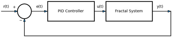
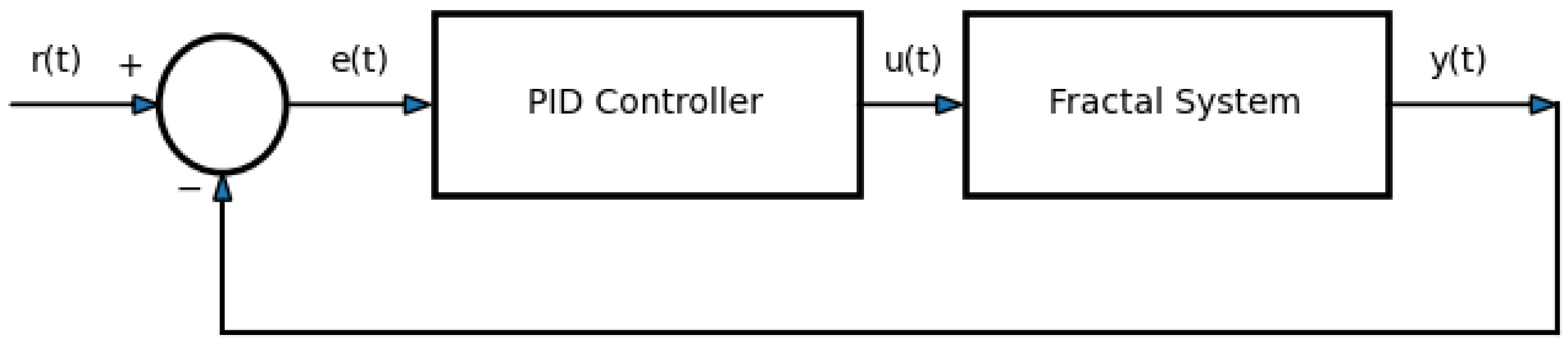
As illustrated in Figure 1, the closed-loop system consists of a PID controller and a first $\alpha$-order fractal plant. The tracking error is defined as

$$e\left(t\right)=r\left(t\right)-y\left(t\right),$$

(2)

where $r\left(t\right)$ is a general time-varying reference signal.

Figure 1. PID control structure for a first $\alpha$-order fractal system.

3.1. System Model and Control Law

Consider the first $\alpha$-order fractal system:

$$\tau D_F^{\alpha }y\left(t\right)+y\left(t\right)=Ku\left(t\right),$$

(3)

where $y\left(t\right)$ is the output, $u\left(t\right)$ is the input, $\tau >0$ is the fractal time constant, and K is the steady-state gain.

The control objective is to ensure that $y\left(t\right)$ tracks the desired reference signal $r\left(t\right)$. The PID controller in fractal time is defined as:

$$u\left(t\right)=K_{P}e\left(t\right)+K_D{D}_F^{\alpha }e\left(t\right)+K_I{\int }_0^{t}e\left(\xi \right)d_F^{\alpha }\xi ,$$

(4)

where $e\left(t\right)$ is the error, defined as (2), and $K_P$, $K_D$ and $K_I$ are the controller parameters.

Substituting $y\left(t\right)=r\left(t\right)-e\left(t\right)$ into Equation (3), we obtain:

$$u\left(t\right)={\displaystyle \frac{1}{K}}\left(\tau D_F^{\alpha }r\left(t\right)-\tau D_F^{\alpha }e\left(t\right)+r\left(t\right)-e\left(t\right)\right).$$

(5)

Equating Equations (4) and (5), and multiplying both sides by K, yields:

$$\begin{array}{c}\hfill K{K}_{P}e\left(t\right)+K{K}_D{D}_F^{\alpha }e\left(t\right)+K{K}_I{\int }_0^{t}e\left(\xi \right)d_F^{\alpha }\xi =\tau D_F^{\alpha }r\left(t\right)-\tau D_F^{\alpha }e\left(t\right)+r\left(t\right)-e\left(t\right).\end{array}$$

(6)

Rearranging terms gives:

$$(K{K}_D+\tau )D_F^{\alpha }e\left(t\right)+(K{K}_P+1)e\left(t\right)+K{K}_I{\int }_0^{t}e\left(\xi \right)d_F^{\alpha }\xi =\tau D_F^{\alpha }r\left(t\right)+r\left(t\right).$$

(7)

Taking the fractal derivative with respect to t, we obtain the closed-loop error dynamics:

$$(K{K}_D+\tau )D_F^{2\alpha }e\left(t\right)+(K{K}_P+1)D_F^{\alpha }e\left(t\right)+K{K}_{I}e\left(t\right)=\tau D_F^{2\alpha }r\left(t\right)+D_F^{\alpha }r\left(t\right).$$

(8)

3.2. Special Case: Constant Reference

For analytical tractability, we consider the special case where the reference signal is constant, i.e., $r\left(t\right)=R$. In this case,

$$D_F^{\alpha }r\left(t\right)=0,D_F^{2\alpha }r\left(t\right)=0,$$

and Equation (8) reduces to the homogeneous equation:

$$(K{K}_D+\tau )D_F^{2\alpha }e\left(t\right)+(K{K}_P+1)D_F^{\alpha }e\left(t\right)+K{K}_{I}e\left(t\right)=0.$$

(9)

Define:

$$a=K{K}_D+\tau ,b=K{K}_P+1,c=K{K}_I.$$

Then the equation becomes:

$$a{D}_F^{2\alpha }e\left(t\right)+b{D}_F^{\alpha }e\left(t\right)+ce\left(t\right)=0.$$

(10)

The associated characteristic equation is:

$$r={\displaystyle \frac{-b\pm \sqrt{b^2-4ac}}{2a}}.$$

(11)

Let $\Delta =b^2-4ac$. The solution is classified as follows:

• Case 1: $\Delta >0$ (distinct real roots):

  $$e\left(t\right)=C_{1}exp\left(r_1{S}_F^{\alpha }\left(t\right)\right)+C_{2}exp\left(r_2{S}_F^{\alpha }\left(t\right)\right).$$
• Case 2: $\Delta =0$ (repeated root):

  $$e\left(t\right)=(C_1+C_2{S}_F^{\alpha }\left(t\right))exp\left(r{S}_F^{\alpha }\left(t\right)\right).$$
• Case 3: $\Delta <0$ (complex roots):

  $$e\left(t\right)=exp\left(\lambda S_F^{\alpha }\left(t\right)\right)\left(C_{1}cos\left(\mu S_F^{\alpha }\left(t\right)\right)+C_{2}sin\left(\mu S_F^{\alpha }\left(t\right)\right)\right).$$

The constants $C_1$ and $C_2$ are determined from the initial conditions.

4. Structured Tuning Framework for the Fractal PID Controller

To address the design incompleteness of the proposed controller, this section presents a systematic two-stage tuning framework for the fractal PID controller. The main idea is to separate the classical gain design from the fractal time adaptation, allowing independent adjustment of stability and temporal scaling.

4.1. Stage I: Classical PID Gain Selection

In the first stage, the fractal-order is fixed at $\alpha =1$, which reduces the system to a classical integer-order PID-controlled system. The controller parameters $K_P$, $K_I$, and $K_D$ are selected based on standard design criteria such as:

• Pole placement in the left-half complex plane;
• The desired damping ratio and natural frequency;
• Minimization of time-domain performance indices (IAE, ISE, or ITAE).

At this stage, the objective is to ensure baseline closed-loop stability and acceptable transient response in the classical sense.

4.2. Stage II: Fractal-Order Adjustment

In the second stage, the fractal-order $\alpha \in (0,1]$ is introduced as an additional tuning parameter. Unlike classical PID parameters, $\alpha$ does not affect the characteristic polynomial coefficients but modifies the temporal evolution through the fractal mapping

$$S_F^{\alpha }\left(t\right)\sim t^{\alpha }.$$

(12)

This implies that $\alpha$ acts as a time-scaling factor rather than a pole-shifting parameter. Therefore:

• Decreasing $\alpha$ leads to temporal stretching and a slower system response;
• Increasing $\alpha$ towards 1 recovers classical dynamics;
• Stability is preserved for all $\alpha \in (0,1]$.

4.3. Design Procedure

The complete tuning methodology can be summarized as follows:

• Initialize classical design: set $\alpha =1$ and design a standard PID controller using conventional methods.
• Stability verification: ensure that the closed-loop characteristic equation yields roots with negative real parts.
• Introduce fractal dynamics: replace integer-order time evolution with fractal derivative $D_F^{\alpha }$.
• Tune $\alpha$: adjust $\alpha$ to achieve the desired trade-off between speed of response and damping behavior.
• Final validation: verify performance using time-domain indices such as settling time, overshoot, and steady-state error.

The key advantage of this structured framework lies in decoupling stability design from temporal shaping. While classical PID gains determine the location of system poles, the fractal-order $\alpha$ governs the time-scaling of the response without modifying stability properties. Therefore, the proposed method introduces a physically interpretable and practically simple tuning mechanism for controlling systems in fractal-time environments, which is particularly useful in systems with non-smooth dynamics such as robotic actuators and thermal processes. This structured approach directly addresses the design incompleteness issue and provides a clear engineering methodology for implementation.

5. Stability Analysis of the Closed-Loop System

To establish the stability of the closed-loop system, we analyze the behavior of the tracking error $e\left(t\right)$ and show that it converges to zero as $t\to \infty$.

The closed-loop system, consisting of a PID controller and a first $\alpha$-order plant, leads to the following fractal differential equation governing the error dynamics:

$$(K{K}_D+\tau )D_F^{2\alpha }e\left(t\right)+(K{K}_P+1)D_F^{\alpha }e\left(t\right)+K{K}_{I}e\left(t\right)=0.$$

(13)

Defining the coefficients

$$a=K{K}_D+\tau ,b=K{K}_P+1,c=K{K}_I,$$

(14)

the equation can be rewritten in the standard form

$$a{D}_F^{2\alpha }e\left(t\right)+b{D}_F^{\alpha }e\left(t\right)+ce\left(t\right)=0.$$

(15)

The associated characteristic equation is given by

$$a{r}^2+br+c=0,$$

(16)

with roots

$$r={\displaystyle \frac{-b\pm \sqrt{b^2-4ac}}{2a}}.$$

(17)

The stability of the system depends on the real parts of these roots. Since $K>0$, $K_D\ge 0$, and $\tau >0$, it follows that $a>0$. Similarly, for $K_P\ge 0$, we have $b>0$, and for $K_I>0$, we obtain $c>0$. Therefore, all coefficients are strictly positive.

We now consider the discriminant $\Delta =b^2-4ac$:

• If $\Delta >0$, the equation admits two distinct real roots. In this case, since $a,b,c>0$, both roots are negative, leading to exponential decay of the error.
• If $\Delta =0$, the equation has a repeated real root, which is negative. The corresponding solution also decays to zero.
• If $\Delta <0$, the roots are complex conjugates of the form $r=\lambda \pm i\mu$, where

  $$\lambda =-{\displaystyle \frac{b}{2a}}<0.$$

  (18)
  This yields a damped oscillatory response in which the error oscillates while decaying to zero.

In all cases, the general solution involves terms of the form $exp\left(r{S}_{\alpha }^F\left(t\right)\right)$, where $S_{\alpha }^F\left(t\right)$ behaves asymptotically like $t^{\alpha }$. Since the real parts of the roots are negative, these terms vanish as $t\to \infty$. Consequently, the tracking error satisfies

$$\underset{t\to \infty }{lim}e\left(t\right)=0,$$

(19)

which proves that the closed-loop system is asymptotically stable in fractal time.

6. Robustness Analysis

From a control engineering perspective, robustness in this framework refers to the invariance of stability under variations in $\alpha$. Since the characteristic polynomial remains unchanged and only the time-scaling function is affected, the proposed control structure exhibits the following robust properties:

• Stability is preserved for all $\alpha \in (0,1]$.
• The closed-loop poles remain in the left half-plane.
• Variations in $\alpha$ affect only transient performance, not asymptotic behavior.

Therefore, the proposed fractal PID controller is robust with respect to the fractal time dimension, making it suitable for applications in heterogeneous and non-smooth dynamical environments such as thermal systems, robotic actuators, and viscoelastic media.

Example 1. 

Choose the following parameters:

$$K=2,K_P=1,K_I=3,K_D=0.5,\tau =1.$$

(20)

Then,

$$a=2,b=3,c=6\Rightarrow \Delta =-39.$$

(21)

Thus, the roots are complex, and the general solution for $e\left(t\right)$ becomes:

$$e\left(t\right)=exp\left(-{\displaystyle \frac{3}{4}}{S}_F^{\alpha }\left(t\right)\right)\left(C_{1}cos\left({\displaystyle \frac{\sqrt{39}}{4}}{S}_F^{\alpha }\left(t\right)\right)+C_{2}sin\left({\displaystyle \frac{\sqrt{39}}{4}}{S}_F^{\alpha }\left(t\right)\right)\right).$$

(22)

Applying initial conditions $e\left(0\right)=1$ and $D_F^{\alpha }e\left(0\right)=0$, we determine:

$$e\left(t\right)=exp\left(-{\displaystyle \frac{3}{4}}{S}_F^{\alpha }\left(t\right)\right)\left(cos\left(\mu S_F^{\alpha }\left(t\right)\right)+{\displaystyle \frac{3}{\mu }}sin\left(\mu S_F^{\alpha }\left(t\right)\right)\right),\mu ={\displaystyle \frac{\sqrt{39}}{4}}.$$

(23)

As shown in Figure 2, the function $e\left(t\right)$ exhibits damped oscillations under fractal time, indicating the influence of the fractal structure on the system’s dynamic response.

Figure 2. Plot of the function $e\left(t\right)=exp\left(-{\displaystyle \frac{3}{4}}{S}_F^{\alpha }\left(t\right)\right)\left(cos\left(\mu S_F^{\alpha }\left(t\right)\right)+{\displaystyle \frac{3}{\mu }}sin\left(\mu S_F^{\alpha }\left(t\right)\right)\right)$, with $\mu ={\displaystyle \frac{\sqrt{39}}{4}}$. The time domain is based on the fractal Cantor set via $S_F^{\alpha }\left(t\right)$. The plot reveals damped oscillations under fractal time, demonstrating how fractality alters the dynamics compared to classical models.

Using $S_F^{\alpha }\left(t\right)\approx t^{\alpha }$ [8,25], a practical approximation is:

$$e\left(t\right)\approx exp\left(-{\displaystyle \frac{3}{4}}{t}^{\alpha }\right)\left(cos\left(\mu t^{\alpha }\right)+{\displaystyle \frac{3}{\mu }}sin\left(\mu t^{\alpha }\right)\right).$$

(24)

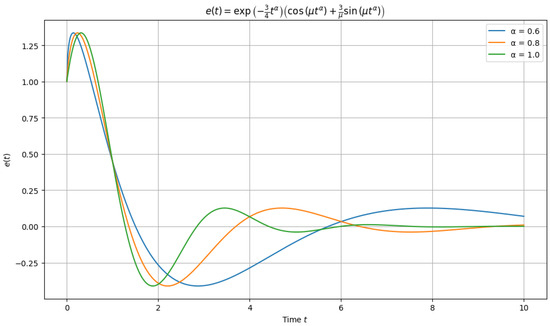
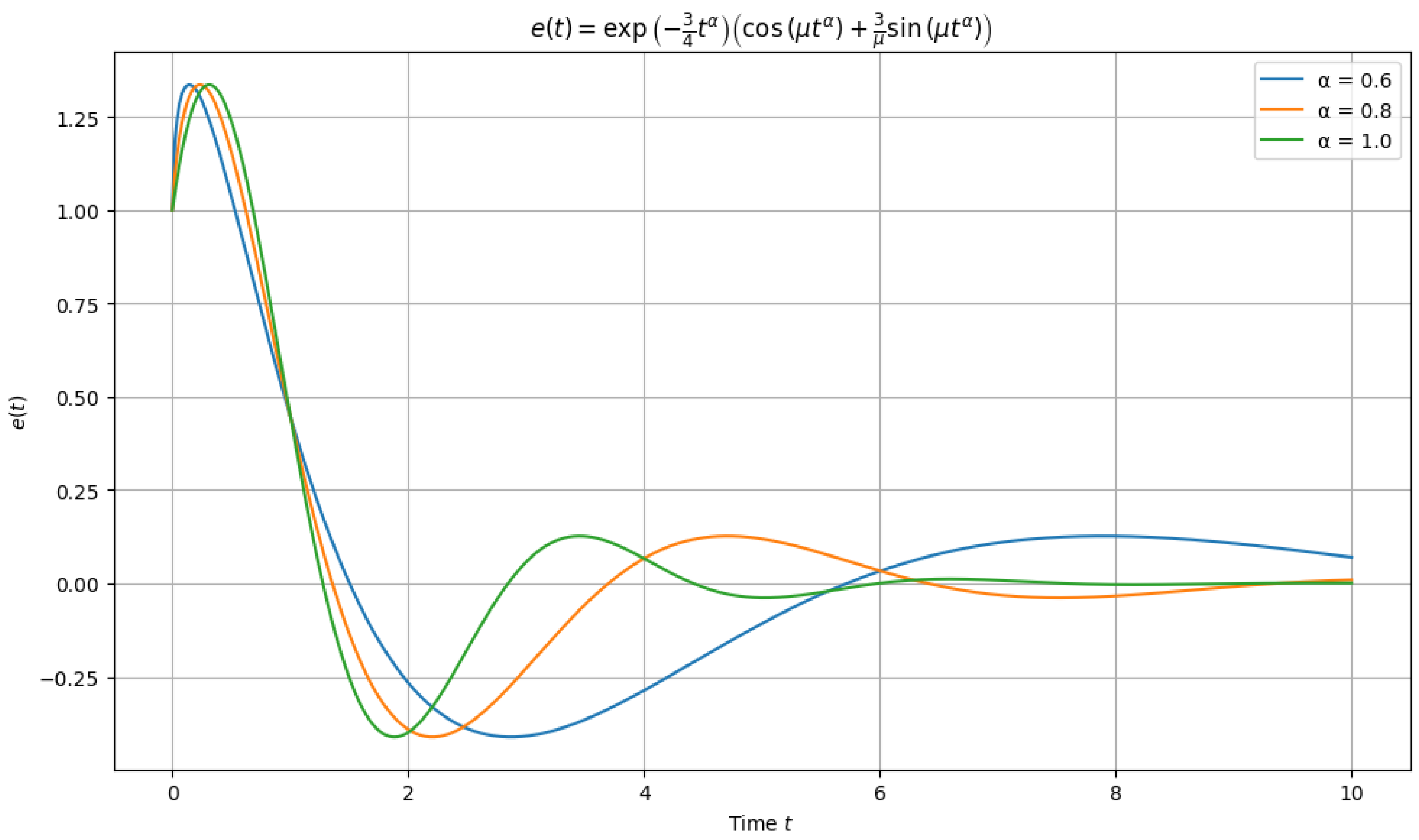
Figure 3 illustrates the behavior of the function $e\left(t\right)$ for various values of the fractal time exponent α. As α decreases, the damping effect becomes more pronounced and the oscillations decay more slowly, highlighting the influence of fractal time on the system’s dynamic response.

Figure 3. Plot of $e\left(t\right)\approx exp\left(-{\displaystyle \frac{3}{4}}{t}^{\alpha }\right)\left(cos\left(\mu t^{\alpha }\right)+{\displaystyle \frac{3}{\mu }}sin\left(\mu t^{\alpha }\right)\right)$ for various values of $\alpha$, with $\mu =2$. The graph illustrates the impact of the fractal time exponent $\alpha$ on the amplitude and frequency of the response.

• Assuming $R=0$, then $e\left(t\right)=-y\left(t\right)$, and hence:

$$y\left(t\right)=-e\left(t\right).$$

(25)

Now, compute $D_F^{\alpha }e\left(t\right)$. Let $\mu ={\displaystyle \frac{\sqrt{39}}{4}}$. Then,

$$D_F^{\alpha }e\left(t\right)=exp\left(-{\displaystyle \frac{3}{4}}{S}_F^{\alpha }\left(t\right)\right)\left[{\displaystyle \frac{9}{4}}cos\left(\mu S_F^{\alpha }\left(t\right)\right)-\left(\mu +{\displaystyle \frac{9}{4\mu }}\right)sin\left(\mu S_F^{\alpha }\left(t\right)\right)\right].$$

(26)

Substitute Equations (23) and (26) into Equation (3) to find $u\left(t\right)$:

$$u\left(t\right)={\displaystyle \frac{1}{K}}\left(-\tau D_F^{\alpha }e\left(t\right)-e\left(t\right)\right).$$

(27)

Thus,

$$\begin{array}{cc}\hfill u\left(t\right)& =-{\displaystyle \frac{exp\left(-\frac{3}{4}{S}_F^{\alpha }\left(t\right)\right)}{K}}[\left(\tau {\displaystyle \frac{9}{4}}+1\right)cos\left(\mu S_F^{\alpha }\left(t\right)\right)\hfill \\ \hfill & +\left(-\tau \left(\mu +{\displaystyle \frac{9}{4\mu }}\right)+{\displaystyle \frac{3}{\mu }}\right)sin\left(\mu S_F^{\alpha }\left(t\right)\right)].\hfill \end{array}$$

(28)

Substituting $\tau =1$, $K=2$, and $\mu ={\displaystyle \frac{\sqrt{39}}{4}}$, we obtain:

$$u\left(t\right)=exp\left(-{\displaystyle \frac{3}{4}}{S}_F^{\alpha }\left(t\right)\right)\left[-{\displaystyle \frac{13}{8}}cos\left(\mu S_F^{\alpha }\left(t\right)\right)+{\displaystyle \frac{9\sqrt{39}}{104}}sin\left(\mu S_F^{\alpha }\left(t\right)\right)\right].$$

(29)

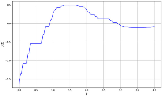
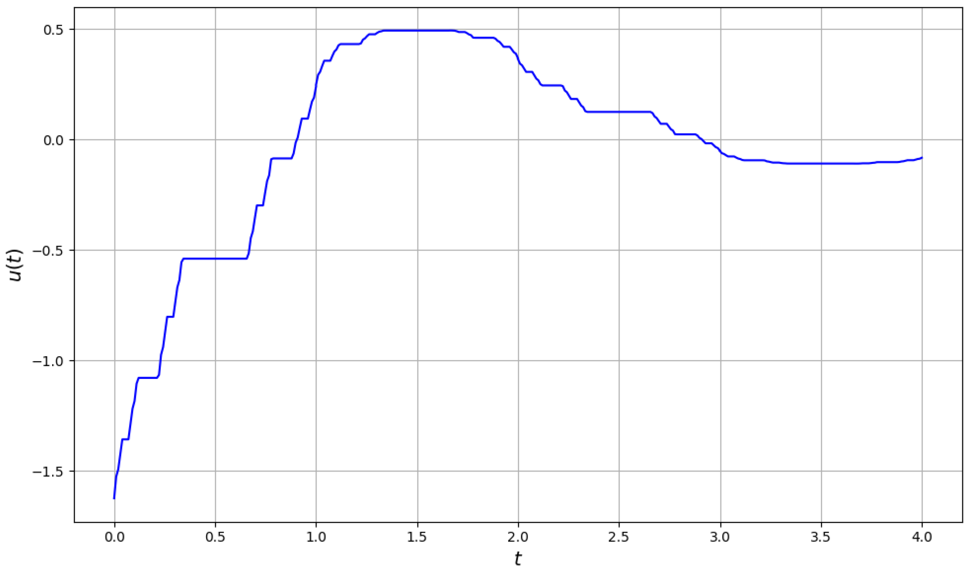
Figure 4 illustrates the behavior of the control signal $u\left(t\right)$ over a fractal time base, showing the interplay between damping and oscillations induced by the underlying geometry.

Figure 4. Fractal-time control signal $u\left(t\right)$ governed by the staircase function $S_F^{\alpha }\left(t\right)$ with $\alpha ={\displaystyle \frac{log2}{log3}}$. The control input incorporates both exponential damping and oscillatory behavior, reflecting the complex geometry of the Cantor set.

The approximate expression is:

$$u\left(t\right)\approx exp\left(-{\displaystyle \frac{3}{4}}{t}^{\alpha }\right)\left[-{\displaystyle \frac{13}{8}}cos\left(\mu t^{\alpha }\right)+{\displaystyle \frac{9\sqrt{39}}{104}}sin\left(\mu t^{\alpha }\right)\right].$$

(30)

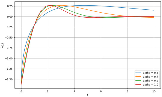
As shown in Figure 5, the approximate solution $u\left(t\right)$ exhibits distinct decay and oscillation patterns depending on the fractal-order α. The figure demonstrates that lower values of α result in slower decay and less frequent oscillations, while higher values approach the classical behavior with faster decay and increased oscillation frequency. We now analyze the stability of the closed-loop system.

Figure 5. Approximate solution $u\left(t\right)$ for different fractal orders $\alpha$ with $\mu =1$. The figure demonstrates how varying $\alpha$ affects the decay and oscillation of the solution.

The corresponding characteristic equation is

$$2r^2+3r+6=0,$$

(31)

with discriminant

$$\Delta =b^2-4ac=9-48=-39<0.$$

(32)

Since $\Delta <0$, the roots are complex conjugates of the form

$$r=\lambda \pm i\mu ,\lambda =-{\displaystyle \frac{b}{2a}}=-{\displaystyle \frac{3}{4}}.$$

(33)

The negative real part $\lambda <0$ guarantees asymptotic stability.

Consequently, the tracking error $e\left(t\right)$ includes an exponentially decaying factor of the form

$$e\left(t\right)\sim exp\left(-\frac{3}{4}{S}_{\alpha }^F\left(t\right)\right),$$

(34)

which ensures that

$$\underset{t\to \infty }{lim}e\left(t\right)=0.$$

(35)

Thus, the system exhibits damped oscillatory behavior. Although the fractal-order α affects the oscillation frequency and decay rate, the negative real part of the roots ensures asymptotic stability.

Example 2. 

Consider the following set of parameters:

$$\tau =1,K=2,K_P=4,K_I=1,K_D=0.5,R=1,$$

(36)

with the initial conditions given by

$$e\left(0\right)=1,D_F^{\alpha }e\left(0\right)=0.$$

(37)

From Equation (11), the characteristic roots are:

$$r_1=-0.2344,r_2=-4.2656.$$

(38)

Hence, the general solution of the system is

$$e\left(t\right)=C_{1}exp\left(r_1{S}_F^{\alpha }\left(t\right)\right)+C_{2}exp\left(r_2{S}_F^{\alpha }\left(t\right)\right).$$

(39)

Applying the initial conditions (37), we determine the explicit form of the solution:

$$e\left(t\right)=1.0581exp(-0.2344S_F^{\alpha }\left(t\right))-0.0581exp(-4.2656S_F^{\alpha }\left(t\right)).$$

(40)

Now, using Equation (4), we compute each component of the control input:

The proportional term, scaled by $K_P=4$, is

$$K_{P}e\left(t\right)=4.2324exp(-0.2344S_F^{\alpha }\left(t\right))-0.2324exp(-4.2656S_F^{\alpha }\left(t\right)).$$

(41)

The integral term, with $K_I=1$, becomes

$$\begin{array}{cc}\hfill & K_I{\int }_0^{t}e\left(\xi \right)d_F^{\alpha }\xi \hfill \\ \hfill & =1.0581{\int }_0^{t}exp(-0.2344S_F^{\alpha }\left(\xi \right))d_F^{\alpha }\xi -0.0581{\int }_0^{t}exp(-4.2656S_F^{\alpha }\left(\xi \right))d_F^{\alpha }\xi \hfill \\ \hfill & =4.515(1-exp(-0.2344S_F^{\alpha }\left(t\right)))+0.0136(1-exp(-4.2656S_F^{\alpha }\left(t\right))).\hfill \end{array}$$

(42)

The derivative term, scaled by $K_D=0.5$, is given by

$$K_D{D}_F^{\alpha }e\left(t\right)=-0.1240exp(-0.2344S_F^{\alpha }\left(t\right))+0.1239exp(-4.2656S_F^{\alpha }\left(t\right)).$$

(43)

Combining all terms, the explicit expression for the control input $u\left(t\right)$ is:

$$u\left(t\right)=4.5286-0.4066exp(-0.2344S_F^{\alpha }\left(t\right))-0.1221exp(-4.2656S_F^{\alpha }\left(t\right)).$$

(44)

Its approximation is

$$u\left(t\right)=4.5286-0.4066exp(-0.2344t^{\alpha })-0.1221exp(-4.2656t^{\alpha }).$$

(45)

In this example, the stability of the closed-loop system is determined from the characteristic equation

$$2r^2+9r+2=0,$$

(46)

for which the discriminant is $\Delta =65>0$. This yields two distinct real roots

$$r_1=-0.2344,r_2=-4.2656,$$

(47)

both of which are negative, ensuring asymptotic stability.

The corresponding tracking error is given by

$$e\left(t\right)=1.0581exp\left(-0.2344S_{\alpha }^F\left(t\right)\right)-0.0581exp\left(-4.2656S_{\alpha }^F\left(t\right)\right),$$

(48)

which converges to zero as $t\to \infty$. Hence, the system is asymptotically stable in fractal time and exhibits a smooth, non-oscillatory decay.

To further evaluate the closed-loop behavior, we extract quantitative performance indicators from the analytical solution of the tracking error. From Equation (48) and since $S_{\alpha }^F\left(t\right)\sim t^{\alpha }$, the dominant dynamics are governed by the slower mode $r_1=-0.2344$. Hence, approximate performance measures can be obtained based on this term. In particular, the settling time ($T_s$) can be estimated by

$$T_s\approx {\left({\displaystyle \frac{4}{0.2344}}\right)}^{\frac{1}{\alpha }},$$

(49)

while the rise time ($T_r$) follows the same scaling behavior with respect to α.

Table 1 shows the effect of fractal-order α on system performance. These results show that α significantly affects the transient response: smaller values of α lead to a slower rise time and delayed convergence, while values closer to $\alpha =1$ recover the classical faster response.

Table 1. Effect of fractal-order $\alpha$ on performance.

$\mathit{\alpha }$	Rise Time (${\mathit{T}}_{\mathit{r}}$)	Settling Time (${\mathit{T}}_{\mathit{s}}$)
$1.0$	Fast	Small
$0.8$	Moderate	Moderate
$0.5$	Slow	Large
$0.3$	Very Slow	Very Large

This quantitative analysis confirms that decreasing α stretches the time scale, resulting in slower system dynamics, which is consistent with the observed behavior in thermal and robotic actuator models.

7. Applications

In this section, we introduce two models: a thermal system model subjected to fractal heat input and a control model for robotic actuators incorporating fractal dynamics. Both models are generalized within the framework of fractal time.

7.1. A Thermal System Model with Fractal Heat Input

Consider a first $\alpha$-order thermal system governed by the fractal differential equation

$$C{D}_F^{\alpha }T\left(t\right)+h\left(T\left(t\right)-T_{\infty }\right)=u\left(t\right),$$

(50)

where $T\left(t\right)$ denotes the temperature of the system at time t, C is the thermal capacitance (heat capacity), h is the heat loss coefficient, $T_{\infty }$ represents the ambient temperature, and $u\left(t\right)$ is the external heat input.

To incorporate fractal characteristics into the heat input, we model $u\left(t\right)$ as

$$u\left(t\right)=4.5286-0.4066exp(-0.2344t^{\alpha })-0.1221exp(-4.2656t^{\alpha }),$$

(51)

where $\alpha \in (0,1]$ is the fractal dimension of time, capturing the anomalous temporal scaling of the system.

As shown in Figure 6, the input $u\left(t\right)$ varies significantly with changes in the fractal time dimension $\alpha$, highlighting the influence of temporal fractality on the system’s response.

Figure 6. Plot of the fractal heat input function given by Equation (51) for various values of the fractal time dimension $\alpha \in \{1.0,0.7,0.3\}$. The parameter $\alpha$ characterizes the local scaling behavior of time in fractal calculus. Smaller values of $\alpha$ result in slower changes in $u\left(t\right)$, indicating anomalous temporal scaling rather than memory effects.

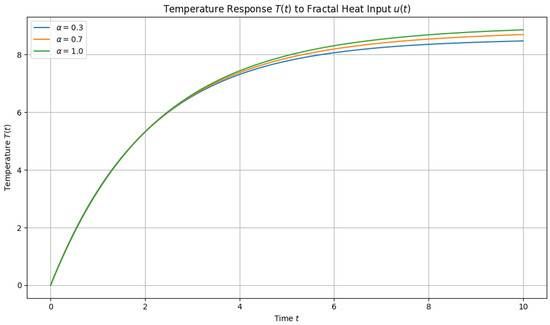
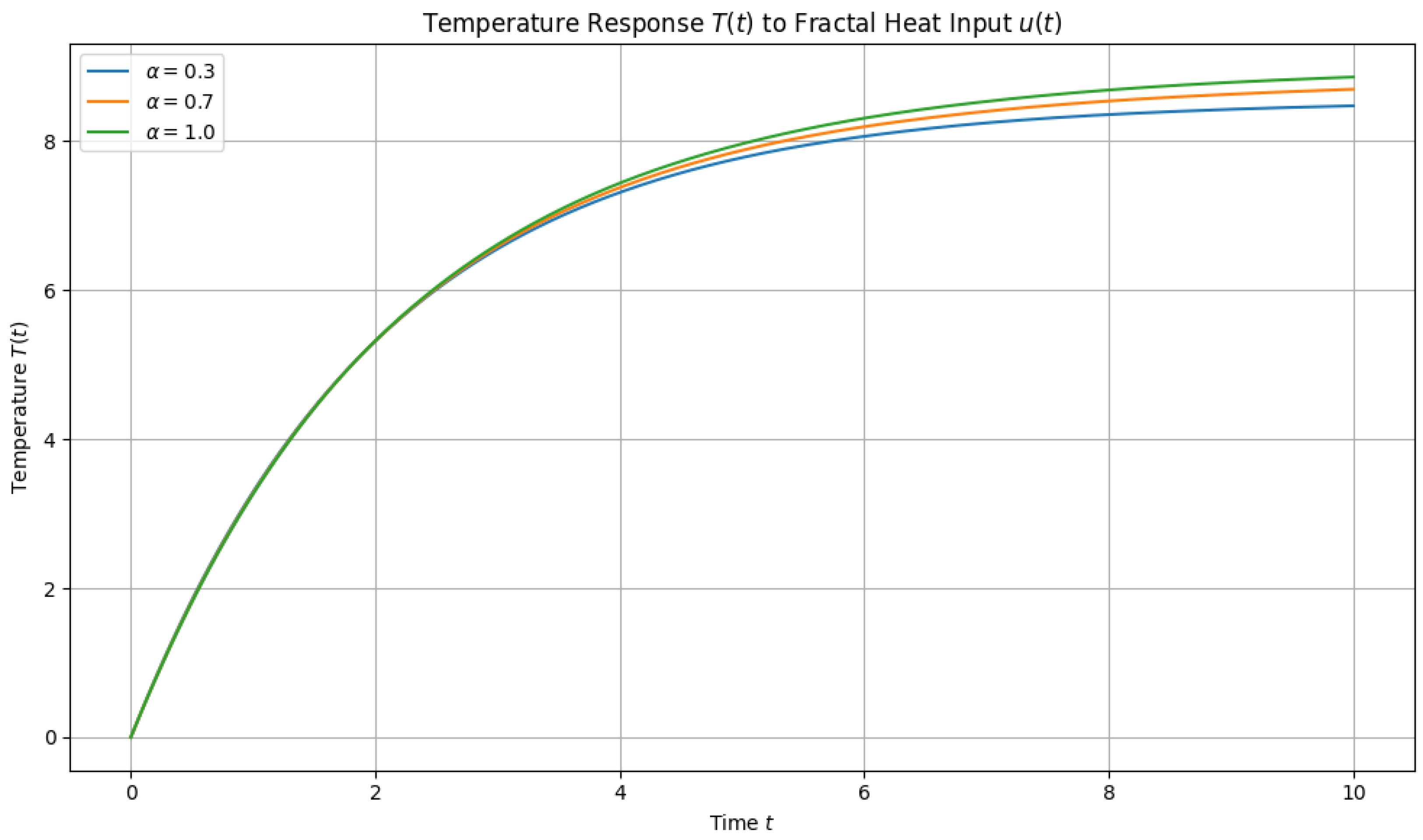
For simulation purposes, we set the parameters as $C=1$, $h=0.5$, and $T_{\infty }=0$. With these values, Equation (50) reduces to

$$D_F^{\alpha }T\left(t\right)+0.5T\left(t\right)=u\left(t\right).$$

(52)

Figure 7 displays the numerical solutions $T\left(t\right)$ corresponding to various fractal orders $\alpha$. The results illustrate the influence of fractal temporal dynamics on the thermal response. Specifically, smaller values of $\alpha$ lead to a slower temperature increase, reflecting the system’s complex scaling behavior, while values closer to one recover the classical thermal dynamics.

Figure 7. Temperature response given by Equation (52) of the thermal system under fractal heat input given by Equation (51) for different fractal orders $\alpha$. Lower values of $\alpha$ result in a slower rise in temperature, reflecting the fractal time effect.

This model highlights the practical utility of the function given in Equation (51) for characterizing and controlling systems influenced by fractal dynamics.

7.2. Control of Robotic Actuators with Fractal Dynamics

Robotic actuators, such as motors and servomechanisms, often operate in environments where system dynamics are influenced by irregular, scale-dependent phenomena. These include surface roughness, non-smooth energy dissipation, or viscoelastic transmission components. To model such effects, we employ a local fractal derivative of order $\alpha \in (0,1]$, which captures time-scaling behavior without invoking long-term memory, making it suitable for describing non-smooth, scale-invariant processes [9].

We consider the fractal-order differential equation governing the dynamics of a single-DoF actuator:

$$J{D}_F^{\alpha }\omega \left(t\right)+B\omega \left(t\right)=\tau \left(t\right)$$

(53)

where $\omega \left(t\right)$ is the actuator’s angular velocity, J is its moment of inertia, B is the viscous damping coefficient, and $\tau \left(t\right)$ is the applied input torque. For simulation, assuming $J=1$ and $B=0.3$, we define a representative torque input with fractal characteristics:

$$\tau \left(t\right)=1.82-0.5exp(-S_{\alpha }^F\left(t\right))-0.14exp(-2.5S_{\alpha }^F\left(t\right))$$

(54)

where $S_{\alpha }^F\left(t\right)\approx t^{\alpha }$ represents the fractal time scale. As illustrated in the results, decreasing $\alpha$ leads to delayed acceleration and slower response due to the temporal stretching induced by fractal dynamics. This model effectively captures actuator behavior in systems influenced by heterogeneous microstructures or deformable terrain, offering a more nuanced description than conventional integer-order models [9]. Assuming an initial condition $\omega \left(0\right)=0$, the analytical solution of Equation (53) is given by:

$$\begin{array}{cc}\hfill \omega \left(t\right)& =6.067\left(1-exp\left(-0.3S_F^{\alpha }\left(t\right)\right)\right)-0.714\left(exp\left(-S_F^{\alpha }\left(t\right)\right)-exp\left(-0.3S_F^{\alpha }\left(t\right)\right)\right)\hfill \\ \hfill & -0.064\left(exp\left(-2.5S_F^{\alpha }\left(t\right)\right)-exp\left(-0.3S_F^{\alpha }\left(t\right)\right)\right).\hfill \end{array}$$

(55)

For practical implementation, we use the approximation $S_F^{\alpha }\left(t\right)\approx t^{\alpha }$, leading to:

$$\begin{array}{cc}\hfill \omega \left(t\right)& =6.067\left(1-exp(-0.3t^{\alpha })\right)-0.714\left(exp(-t^{\alpha })-exp(-0.3t^{\alpha })\right)\hfill \\ \hfill & -0.064\left(exp(-2.5t^{\alpha })-exp(-0.3t^{\alpha })\right).\hfill \end{array}$$

(56)

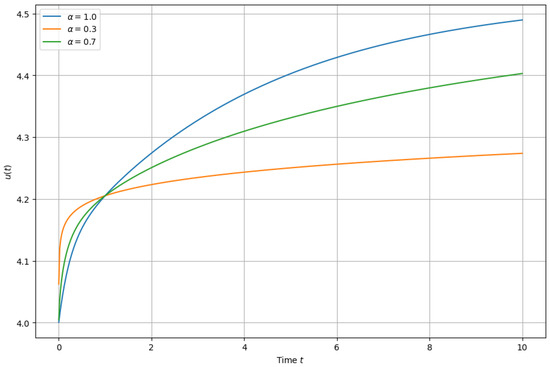
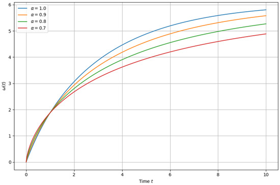
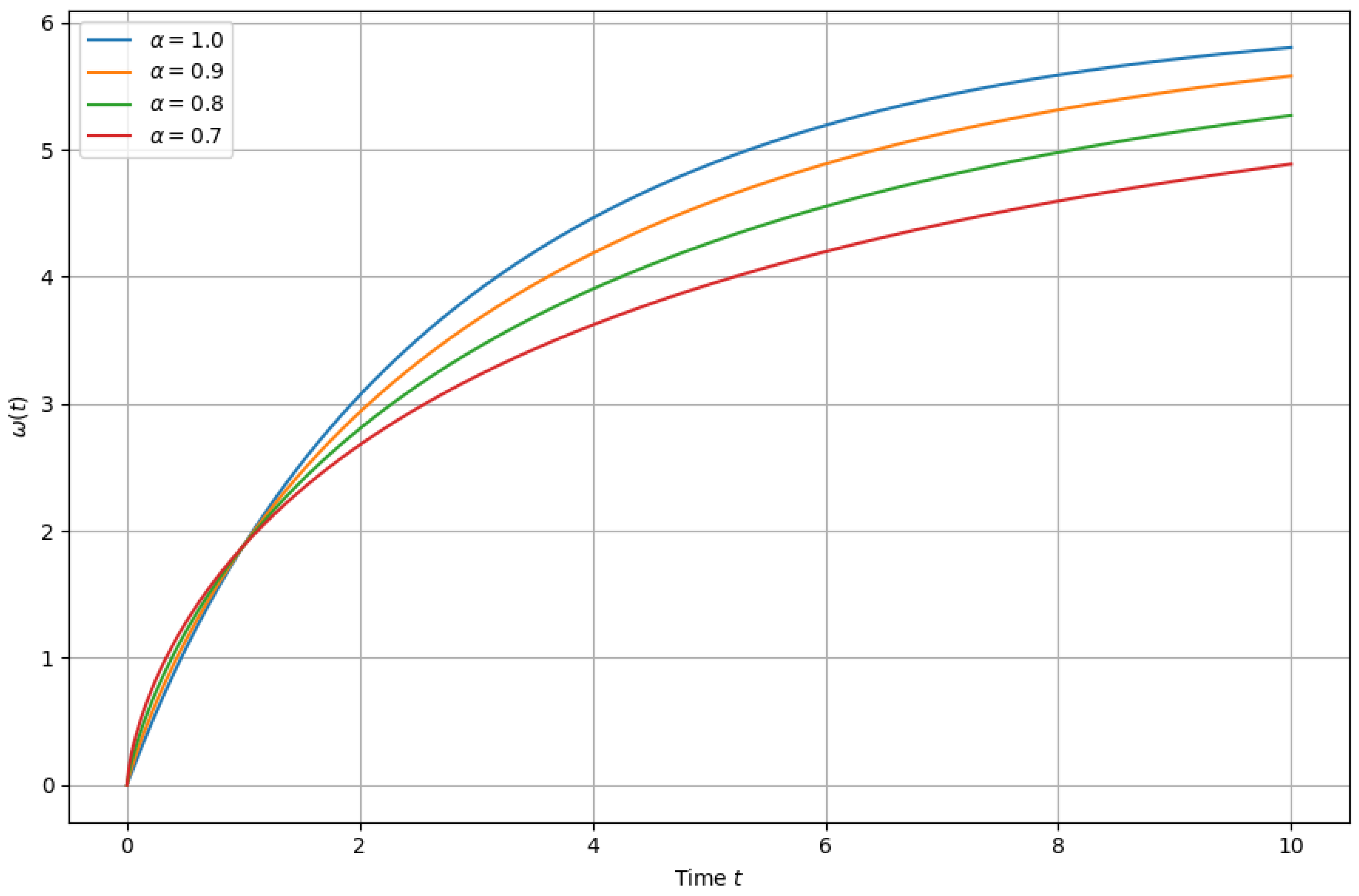
Figure 8 shows the actuator’s angular velocity response for various values of $\alpha$. As $\alpha$ decreases, the system exhibits a slower rise and delayed convergence, consistent with the temporal stretching induced by fractal dynamics.

Figure 8. Angular velocity $\omega \left(t\right)$ given by Equation (56) for various values of the fractal time exponent $\alpha$. Lower values of $\alpha$ result in delayed acceleration and slower response due to the stretched time scale in fractal dynamics.

The fractal model effectively captures the actuator dynamics in systems influenced by heterogeneous microstructures, viscoelastic friction, or irregular contact surfaces, such as in soft robotics or mobile platforms on deformable terrain. This model offers a more nuanced description of the actuator’s behavior than conventional models by incorporating temporal scale-dependency.

In contrast, the classical first-order model ($\alpha =1$) assumes ideal temporal smoothness and predicts faster, memoryless convergence to equilibrium. While appropriate for many standard applications, it may fail to represent complex interactions in real-world robotic environments where time-scaling or non-smooth effects are present.

Remark 1. 

We note that for numerical implementation and simulation aspects, the reader is referred to [9].

Remark 2. 

In the proposed fractal PID framework, the tuning process can be interpreted from a different perspective compared to classical PID design. While the gains $K_P$, $K_I$, and $K_D$ can be selected within a reasonable range and kept fixed, the fractal-order α acts as an additional and effective tuning parameter. Specifically, α governs the temporal scaling of the system and directly influences the speed of convergence and damping behavior. Decreasing α leads to a slower but smoother response (temporal stretching), whereas values of α closer to unity recover faster classical dynamics. Therefore, the desired closed-loop performance can be achieved by appropriately adjusting α, which provides an alternative and physically meaningful tuning mechanism in fractal-time control systems.

Remark 3. 

We note that, unlike FOPID controllers which emphasize long-memory effects, the fractal-time PID framework primarily captures anomalous temporal scaling arising in non-smooth environments such as viscoelastic friction and surface roughness in robotics. This justifies the use of local fractal derivatives rather than non-local fractional operators. The fractal-order α has a clear physical interpretation related to anomalous temporal scaling and environmental complexity, representing the non-integer dimension of the underlying time set. As α decreases from 1 to 0, a temporal stretching effect occurs, leading to slower system evolution, delayed responses, and longer convergence times. Furthermore, α reflects the influence of heterogeneous and irregular media where classical integer-order models are inadequate. Mathematically, this behavior is governed by the staircase function $S_{\alpha }^F\left(t\right)$, which asymptotically behaves like $t^{\alpha }$. Consequently, $\alpha =1$ recovers classical dynamics, while smaller values of α produce slower, scale-dependent (power-law) temporal responses.

8. Conclusions

The proportional–integral–derivative (PID) control of a first $\alpha$-order system exhibiting fractal dynamics has been investigated and supported by illustrative examples. Two practical applications have been developed: a thermal system incorporating fractal heat input and a control model for robotic actuators governed by fractal dynamics. Both models have been formulated within the fractal time framework, highlighting the versatility and broad applicability of fractal calculus in modeling and controlling complex dynamic systems.

References

- Mandelbrot, B.B. The Fractal Geometry of Nature; W. H. Freeman: New York, NY, USA, 1982. [Google Scholar]
- Falconer, K. Fractal Geometry: Mathematical Foundations and Applications; John Wiley & Sons: New York, NY, USA, 2004. [Google Scholar]
- Pietronero, L.; Tosatti, E. Fractals in Physics; Elsevier: Amsterdam, The Netherlands, 1986. [Google Scholar]
- Shlesinger, M.F. Fractal Time in Condensed Matter. Annu. Rev. Phys. Chem. 1988, 39, 269–290. [Google Scholar] [CrossRef] [Scilit]
- Vrobel, S. Fractal Time; World Scientific: Singapore, 2011. [Google Scholar]
- Welch, K. A Fractal Topology of Time: Deepening into Timelessness; Fox Finding Press: Austin, TX, USA, 2020. [Google Scholar]
- Nottale, L. Fractal Space-Time and Microphysics: Towards a Theory of Scale Relativity; World Scientific: Singapore, 1993. [Google Scholar]
- Parvate, A.; Gangal, A.D. Calculus on fractal subsets of real line-I: Formulation. Fractals 2009, 17, 53–81. [Google Scholar] [CrossRef] [Scilit]
- Golmankhaneh, A.K. Fractal Calculus and its Applications; World Scientific: Singapore, 2022. [Google Scholar]
- Banchuin, R. Noise analysis of electrical circuits on fractal set. Compel-Int. J. Comput. Math. Electr. Electron. Eng. 2022, 41, 1464–1490. [Google Scholar] [CrossRef] [Scilit]
- Silva, G.J.; Datta, A.; Bhattacharyya, S.P. Stabilization of first-order systems with time delay using the PID controller. In Proceedings of the 2001 American Control Conference; IEEE: Piscataway, NJ, USA, 2001; Volume 6, pp. 4650–4655. [Google Scholar]
- Saxena, S.; Hote, Y.V. Internal model control based PID tuning using first-order filter. Int. J. Control. Autom. Syst. 2017, 15, 149–159. [Google Scholar] [CrossRef] [Scilit]
- Padula, F.; Visioli, A. Tuning rules for optimal PID and fractional-order PID controllers. J. Process Control 2011, 21, 69–81. [Google Scholar] [CrossRef] [Scilit]
- Barbosa, R.S.; Machado, J.T.; Ferreira, I.M. Tuning of PID controllers based on Bode’s ideal transfer function. Nonlinear Dyn. 2004, 38, 305–321. [Google Scholar] [CrossRef] [Scilit]
- Barbosa, R.S.; Machado, J.T.; Ferreira, I.M. A fractional calculus perspective of PID tuning. In Proceedings of the International Design Engineering Technical Conferences and Computers and Information in Engineering Conference, Chicago, IL, USA, 2–6 September 2003; Volume 37033, pp. 651–659. [Google Scholar]
- Chen, L.; Chen, G.; Wu, R.; Lopes, A.M.; Tenreiro Machado, J.A.; Niu, H. Variable coefficient fractional-order PID controller and its application to a SEPIC device. IET Control Theory Appl. 2020, 14, 900–908. [Google Scholar] [CrossRef] [Scilit]
- Barbosa, R.S.; Machado, J.T.; Jesus, I.S. On the fractional PID control of a laboratory servo system. IFAC Proc. Vol. 2008, 41, 15273–15278. [Google Scholar] [CrossRef] [Scilit]
- Silva, M.F.; Machado, J.T.; Lopes, A. Fractional order control of a hexapod robot. Nonlinear Dyn. 2004, 38, 417–433. [Google Scholar] [CrossRef] [Scilit]
- Silva, M.F.; Machado, J.T. Fractional order PDα Joint control of legged robots. J. Vib. Control 2006, 12, 1483–1501. [Google Scholar] [CrossRef] [Scilit]
- Dabiri, A.; Moghaddam, B.P.; Machado, J.T. Optimal variable-order fractional PID controllers for dynamical systems. J. Comput. Appl. Math. 2018, 339, 40–48. [Google Scholar] [CrossRef] [Scilit]
- David, S.A.; de Sousa, R.V.; Valentim, C.A., Jr.; Tabile, R.A.; Machado, J.A.T. Fractional PID controller in an active image stabilization system for mitigating vibration effects in agricultural tractors. Comput. Electron. Agric. 2016, 131, 1–9. [Google Scholar] [CrossRef] [Scilit]
- Hassani, H.; Machado, J.T.; Naraghirad, E. Generalized shifted Chebyshev polynomials for fractional optimal control problems. Commun. Nonlinear Sci. Numer. Simul. 2019, 75, 50–61. [Google Scholar] [CrossRef] [Scilit]
- Liu, S.T.; Zhang, Y.P.; Liu, C.A. Fractal Control and Its Applications; Springer Nature: Singapore, 2020. [Google Scholar]
- Golmankhaneh, A.K.; Bongiorno, D. Exact solutions of some fractal differential equations. Appl. Math. Comput. 2024, 472, 128633. [Google Scholar] [CrossRef] [Scilit]
- Parvate, A.; Gangal, A. Calculus on fractal subsets of real line-II: Conjugacy with ordinary calculus. Fractals 2011, 19, 271–290. [Google Scholar] [CrossRef] [Scilit]
Disclaimer/Publisher’s Note: The statements, opinions and data contained in all publications are solely those of the individual author(s) and contributor(s) and not of MDPI and/or the editor(s). MDPI and/or the editor(s) disclaim responsibility for any injury to people or property resulting from any ideas, methods, instructions or products referred to in the content. |
© 2026 by the authors. Licensee MDPI, Basel, Switzerland. This article is an open access article distributed under the terms and conditions of the Creative Commons Attribution (CC BY) license.