A Variable-Order ABC Fractional Framework for Systemic Financial Stress Dynamics

Abstract

This paper studies a novel nonlinear fractional-order financial stress model involving Atangana–Baleanu–Caputo (ABC) operators. It focuses on memory effects that are both constant and variable. The novelty of the proposed framework lies in combining multiple interconnected channels of systemic stress into one fractional dynamical model and looks at how they change over time and how they respond to sustained external perturbations. Theoretically, we prove well-posedness results and study the equilibrium structure and stability of the given model. On the computational side, we use numerical simulations of the individual stress components and an aggregate systemic stress index to look into short-term dynamics under different memory regimes. We also include a shock-response analysis to show how memory effects change the way stress builds up, relaxes, and spreads when forced. The sensitivity analysis shows that systemic stress is amplified by the forcing and interaction parameters and reduced by the damping parameters. These findings demonstrate that the model provides a new and effective tool for studying systemic financial instability in a fractional setting.

1. Introduction

Classical integer-order models often fail to accurately represent the inherent complexity of contemporary financial systems, characterized by nonlinear interactions, memory effects, and swift regime transitions [1]. Traditional systemic risk metrics, such as the VIX index or credit default swap spreads, often ignore the fact that financial stress propagates in a non-Markovian way, meaning that past shocks continue to affect future states [2]. This restriction is essential during crises, as systemic failures can be intensified by sluggish policy reactions to liquidity deficits or credit contagion [3].

Fractional calculus is a powerful method for modeling systems with long-range memory and unusual diffusion [4,5,6,7]. In [8,9,10], the variable-order Riemann–Liouville fractional derivative was initially introduced. The authors of [11] examined extended formulations. In a similar way, ref. [12] created the Caputo-type variable-order fractional derivative, and refs. [13,14] showed how it could be expanded even more.

In [15], Yue, He, and Liu introduced a nonlinear fractional financial model with practical applications. Tarasov in [16] discussed the importance of fractional calculus in mathematical economics. Gao, Li, and Wang [17] investigated chaos in a fractional-order financial system. Madani et al. created a generalized fractional cobweb model for market adjustment in [18]. The modeling and study of complex dynamical systems, especially financial systems with path-dependent behavior, have greatly benefited from the invention of fractional calculus [19]. The ABC fractional derivative has become a potent tool for capturing genetic effects in neural networks owing to its non-singular Mittag–Leffler kernel. The ABC operator is particularly advantageous for financial systems as it circumvents kernel singularities, unlike conventional Caputo or Riemann–Liouville derivatives, while preserving the ability to depict power-law memory decay [20,21,22]. Numerous recent studies have looked at variable-order fractional models and their applications. Heydari [23] employed Chebyshev cardinal functions to address the nonlinear optimum control issues involving the ABC variable-order derivative. Zheng et al. [24] investigated a variable-order time-fractional reaction-diffusion model using a Mittag–Leffler kernel. A numerical approach for variable-order fractal-fractional delay equations was developed by Basim et al. [25], and a method for multi-variable order differential equations was proposed by Ganji et al. [26]. Yang [27] used variable-order derivatives to model anomalous thermal relaxation.

Recent studies validate the increasing significance of fractional-order models in economics and finance. Aloui et al. [28] examined a fractional economic system and demonstrated that both constant and variable orders significantly influence chaos and control behavior. Berir [29] investigated a financial fractional model subjected to white noise and discovered that stochastic perturbations affect chaotic dynamics variably in constant- and variable-order contexts. Allogmany et al. [30] further emphasized the more complex dynamic behavior of variable-order fractional systems via a comparative chaos analysis. In financial contexts, Prathumwan et al. [31] demonstrated well-posedness and stability results for an ABC asset-flow model. Sun et al. [32] broadened the focus to systemic risk modeling, demonstrating that fractional frameworks can accurately depict contagion and enhance forecasting within interconnected financial networks. A thorough framework for systemic stress indices is still lacking despite recent research using fractional calculus to volatility modeling [33], option pricing [34], and risk propagation [35].

In this study, we develop a systemic financial-stress framework based on the ABC fractional operator with a time-varying order $\alpha \left(t\right)$, designed to overcome key limitations of classical stress-index models. First, by allowing the fractional order to vary over time, the model adapts dynamically to changes in shock persistence, naturally distinguishing between rapid dissipation in tranquil market regimes and prolonged effects during periods of financial crisis. Second, the proposed dynamics explicitly incorporate nonlinear cross-channel spillovers through multiplicative interaction terms ${\beta }_{ij}$, capturing contagion and amplification mechanisms among market, liquidity, credit, and sentiment stresses.

This paper contributes in four ways. First, we develop a nonlinear fractional-order model involving time-varying order $\alpha \left(t\right)$ with the four main aspects of financial stress. Second, we offer a thorough theoretical analysis of the model, proving that solutions are unique under mild Lipschitz conditions, non-negativity, and boundedness of solutions. Then, obtaining the requirements for the equilibrium’s local asymptotic stability. Third, we provide numerical simulations with different fractional orders. Additionally, we offer impulse-response simulations that show how shocks spread and how the memory parameters affect the system’s ability to return to equilibrium. Fourth, we conduct a local sensitivity analysis, offering the impact of each parameter on the dynamic cumulative stress exposure as well as the equilibrium stress levels. Finally, the detailed partial-equilibrium formulas are deferred to an appendix.

The remainder of this paper is organized as follows: Section 2 offers some fundamental topics related to ABC fractional calculus. In Section 3, we present the formulation of the proposed nonlinear fractional systemic stress model using the ABC derivative with time-varying order $\alpha \left(t\right)$, and provide a theoretical analysis of the model, including well-posedness theorem, non-negativity, and boundednees of solutions. Section 4 discusses the equilibrium and local stability analysis. In Section 5, we develop and implement numerical schemes to solve the model and explore its behavior under various memory and parameter configurations. Section 6 provides the sensitivity analysis. Finally, Section 7 concludes this paper with a discussion of the main results and directions for future research.

2. Basic Results

In the following, we present essential concepts and foundational results in the field of fractional calculus. As usual, $\mathcal{C}:=C(\mathbb{J},{\mathbb{R}}^4)$ is the Banach space of all continuous functions from $\mathbb{J}$ to ${\mathbb{R}}^4$, where $\mathbb{J}=[0,T]$, $T>0$, equipped with the following norm:

$${\parallel \omega \parallel }_{\infty }=\underset{1\le i\le 4}{max}\underset{\nu \in \mathbb{J}}{sup}\left|{\omega }_i\left(\nu \right)\right|.$$

Definition 1

([19]). Consider $\mu \in (0,1]$ and $\omega \in H^1(0,T)$. The left-sided Caputo fractional derivative of order μ in the sense of Atangana–Baleanu for a function ω is expressed as follows:

$${}^{\mathcal{ABC}}\left({\mathcal{D}}_0^{\mu }\omega \right)\left(t\right)={\displaystyle \frac{\Delta \left(\mu \right)}{1-\mu }}{\int }_0^t{E}_{\mu }\left[-{\displaystyle \frac{\mu }{1-\mu }}{(t-\nu )}^{\mu }{\omega }^{\prime }\left(\nu \right)\right]d\nu ,t\in \mathbb{J}.$$

where $\Delta \left(\mu \right)=1-\mu +{\displaystyle \frac{\mu }{\mathrm{\Gamma }\left(\mu \right)}}$ is fulfilling $\Delta \left(0\right)=\Delta \left(1\right)=1$, and $E_{\mu }(·)$ is the Mittag–Leffler function, defined as follows:

$$E_{\mu }\left(\omega \right)={\displaystyle \sum _{i=0}^{\infty }}{\displaystyle \frac{{\omega }^i}{\mathrm{\Gamma }(\mu i+1)}},\mathit{Re}\left(\mu \right)>0,r\in \mathbb{C},$$

where $\mathrm{\Gamma }(·)$ is the Gamma function, defined as $\mathrm{\Gamma }\left(\mu \right)={\int }_0^{\infty }{e}^{-x}{x}^{\mu -1}dx,\mu >0$.

Definition 2

([19]). Consider $\mu \in (0,1]$ and $\omega \in H^1(0,T)$. The left-sided Riemann–Liouville fractional integral of order μ in the sense of Atangana–Baleanu for a function ω is given by:

$${}^{\mathcal{AB}}{\mathcal{I}}_0^{\mu }\omega \left(t\right)={\displaystyle \frac{1-\mu }{\Delta \left(\mu \right)}}\omega \left(t\right)+{\displaystyle \frac{\mu }{\Delta \left(\mu \right)\mathrm{\Gamma }\left(\mu \right)}}{\int }_0^t{(t-\nu )}^{\mu -1}\omega \left(s\right)ds,t\in \mathbb{J}.$$

Definition 3

([23,36]). Let $\alpha :[0,t_{\mathit{max}}]\to (0,1)$ be a continuous function and $\omega \in C^1\left([0,t_{\mathit{max}}]\right)$. Then, the ABC fractional derivative of variable order $\alpha \left(t\right)$ is defined by:

$${}^{ABC}{D}_t^{\alpha \left(t\right)}\omega \left(t\right)={\displaystyle \frac{B\left(\alpha \right(t\left)\right)}{1-\alpha \left(t\right)}}{\int }_0^t{\omega }^{\prime }\left(s\right)E_{\alpha \left(t\right)}\left(-{\displaystyle \frac{\alpha \left(t\right)}{1-\alpha \left(t\right)}}{(t-s)}^{\alpha \left(t\right)}\right)ds,$$

where $E_{\alpha \left(t\right)}(·)$ is the Mittag–Leffler function. Moreover, ${}^{ABC}{D}_t^{\alpha \left(t\right)}C=0$ for any constant C.

Definition 4.

The associated ABC fractional integral of variable order $\alpha \left(t\right)$ is:

$${}^{AB}{I}_t^{\alpha \left(t\right)}f\left(t\right)={\displaystyle \frac{1-\alpha \left(t\right)}{B\left(\alpha \right(t\left)\right)}}f\left(t\right)+{\displaystyle \frac{\alpha \left(t\right)}{B\left(\alpha \right(t\left)\right)\mathrm{\Gamma }\left(\alpha \right(t\left)\right)}}{\int }_0^t{(t-s)}^{\alpha \left(t\right)-1}f\left(s\right)ds.$$

3. Model Analysis

This section focuses on formulating the mathematical model and proving the properties of the model, such as uniqueness, non-negativity, and boundedness of solutions.

3.1. Mathematical Model

ABC-type nonlinear FDEs govern the dynamics of each stress component in the following way:

$$\begin{array}{c}\hfill \left\{\begin{array}{cc}{}^{ABC}{D}_t^{\alpha \left(t\right)}A\left(t\right)\hfill & =-{\lambda }_{A}A\left(t\right)+{\gamma }_A{g}_A\left(t\right)+{\beta }_{AB}B\left(t\right)A\left(t\right)+{\beta }_{AD}D\left(t\right)A\left(t\right),\hfill \\ {}^{ABC}{D}_t^{\alpha \left(t\right)}B\left(t\right)\hfill & =-{\lambda }_{B}B\left(t\right)+{\gamma }_B{g}_B\left(t\right)+{\beta }_{BA}A\left(t\right)B\left(t\right)+{\beta }_{BC}C\left(t\right)B\left(t\right),\hfill \\ {}^{ABC}{D}_t^{\alpha \left(t\right)}C\left(t\right)\hfill & =-{\lambda }_{C}C\left(t\right)+{\gamma }_C{g}_C\left(t\right)+{\beta }_{CB}B\left(t\right)C\left(t\right)+{\beta }_{CD}D\left(t\right)C\left(t\right),\hfill \\ {}^{ABC}{D}_t^{\alpha \left(t\right)}D\left(t\right)\hfill & =-{\lambda }_{D}D\left(t\right)+{\gamma }_D{g}_D\left(t\right)+{\beta }_{DA}A\left(t\right)D\left(t\right)+{\beta }_{DC}C\left(t\right)D\left(t\right).\hfill \end{array}\right.\end{array}$$

(1)

where

• Market Stress ($A\left(t\right)$): captures volatility and price fluctuations.
• Liquidity Stress ($B\left(t\right)$): reflects funding and liquidity shortages.
• Credit Stress ($C\left(t\right)$): measures default risks and credit spreads.
• Sentiment Stress ($D\left(t\right)$): represents investor sentiment and behavioral biases.
• ${\lambda }_A,{\lambda }_B,{\lambda }_C,{\lambda }_D>0$ are decay rates.
• ${\gamma }_A,{\gamma }_B,{\gamma }_C,{\gamma }_D\ge 0$ are shock sensitivity coefficients.
• ${\beta }_{ij}\ge 0$ are nonlinear interaction coefficients.
• $g_A\left(t\right),g_B\left(t\right),g_C\left(t\right),g_D\left(t\right)$ are external shocks.
• $A\left(0\right),B\left(0\right),C\left(0\right),D\left(0\right)\ge 0$ are initial conditions.

The overall systemic stress index $S\left(t\right)$ is a weighted sum of the stress components:

$$S\left(t\right)=w_{A}A\left(t\right)+w_{B}B\left(t\right)+w_{C}C\left(t\right)+w_{D}D\left(t\right),\mathrm{with}\sum _{i=A,B,C,D}{w}_i=1,$$

(2)

and time-varying fractional order is the fractional order $\alpha \left(t\right)$, which evolves over time to reflect changing memory effects:

$$\alpha \left(t\right)={\alpha }_0+{\alpha }_{1}sin\left({\displaystyle \frac{2\pi t}{T}}\right),$$

(3)

where:

• ${\alpha }_0\in (0,1)$ is the baseline memory effect.
• ${\alpha }_1\in [0,{\alpha }_0)$ controls the amplitude of memory variation.
• T is the period of memory variation (e.g., 30 days for monthly cycles).

Now, we present a financial interpretation of the model parameters, as shown in Table 1.

Table 1. Financial interpretation of model parameters.

Parameter	Financial Meaning
${\lambda }_A,{\lambda }_B,{\lambda }_C,{\lambda }_D$	Rate of decay for market, liquidity, credit, and sentiment stress. Higher values indicate faster stabilization of stress.
${\gamma }_A,{\gamma }_B,{\gamma }_C,{\gamma }_D$	Sensitivity of stress components to external shocks. Higher values mean greater responsiveness to sudden changes.
${\beta }_{AB},{\beta }_{AD},{\beta }_{BA},{\beta }_{BC},{\beta }_{CB},{\beta }_{CD},{\beta }_{DA},{\beta }_{DC}$	Interconnectedness between stress types. Higher values reflect stronger feedback effects between components.
$\alpha \left(t\right)$	Memory effect in the system. A higher value indicates slower decay and stronger influence of past stress values.
$w_A,w_B,w_C,w_D$	Weights for each stress component in the overall systemic stress index $S\left(t\right)$. Reflects the contribution of each stress type.
$g_A\left(t\right),g_B\left(t\right),g_C\left(t\right),g_D\left(t\right)$	Magnitude of external shocks. Influences each stress component directly.

3.2. Well-Posedness Theorems

Here, we formalize the well-posedness analysis through three theorems addressing the existence of a unique solution, non-negativity, and boundedness of solutions.

Let $\mathbb{J}=[0,T]$, $T>0$. Consider the following system:

$${}^{ABC}{D}_t^{\alpha \left(t\right)}\mathbf{X}\left(t\right)=\mathbf{F}(t,\mathbf{X}\left(t\right)),\mathbf{X}\left(0\right)={\mathbf{X}}_0\in {\mathbb{R}}^4,$$

where $\mathbf{X}\left(t\right)={\left(A\left(t\right),B\left(t\right),C\left(t\right),D\left(t\right)\right)}^T$, and

$$\begin{array}{c}\hfill \mathbf{F}(t,\mathbf{X})=\left[\begin{array}{c}-{\lambda }_{A}A+{\gamma }_A{g}_A\left(t\right)+{\beta }_{AB}BA+{\beta }_{AD}DA\\ -{\lambda }_{B}B+{\gamma }_B{g}_B\left(t\right)+{\beta }_{BA}AB+{\beta }_{BC}CB\\ -{\lambda }_{C}C+{\gamma }_C{g}_C\left(t\right)+{\beta }_{CB}BC+{\beta }_{CD}DC\\ -{\lambda }_{D}D+{\gamma }_D{g}_D\left(t\right)+{\beta }_{DA}AD+{\beta }_{DC}CD\end{array}\right].\end{array}$$

(4)

Assume that

Hypothesis 1

(H1). $\alpha :\mathbb{J}\to (0,1)$ and $g_i:\mathbb{J}\to \mathbb{R}$ are continuous, for each $i\in \{A,B,C,D\}$.

Hypothesis 2

(H2). $\mathbf{F}$ is continuous on $\mathbb{J}\times {\mathbb{R}}^4$ and locally Lipschitz continuous with respect to $\mathbf{X}$; that is, for every $R>0$, there exists $L_R>0$ such that

$$\parallel \mathbf{F}(t,\mathbf{X})-\mathbf{F}(t,\mathbf{Y})\parallel \le L_R\parallel \mathbf{X}-\mathbf{Y}\parallel ,\forall t\in \mathbb{J},\mathbf{X},\mathbf{Y}\in {\mathbb{B}}_R\left({\mathbf{X}}_0\right),$$

where

$${\mathbb{B}}_R\left({\mathbf{X}}_0\right):=\{\mathbf{X}\in {\mathbb{R}}^4:\hspace{0.17em}\parallel \mathbf{X}-{\mathbf{X}}_0\parallel \le R\}.$$

Hypothesis 3

(H3). There exist $R>0$ and $T_0\in (0,T]$ such that the integral operator associated with the ABC formulation maps

$$\mathcal{S}:=\left\{\mathbf{X}\in C([0,T_0],{\mathbb{R}}^4):\underset{t\in [0,T_0]}{sup}\parallel \mathbf{X}\left(t\right)-{\mathbf{X}}_0\parallel \le R\right\}$$

into itself and satisfies $L_{R}C\left(T_0\right)<1,$ where $C\left(T_0\right)$ is the constant obtained from the ABC integral estimate.

Theorem 1

(Local existence and uniqueness). Under Hypotheses H1–H3, the system (1) admits a unique solution

$$\mathbf{X}\left(t\right)={\left(A\left(t\right),B\left(t\right),C\left(t\right),D\left(t\right)\right)}^T$$

on the interval $[0,T_0]$.

Proof. 

The proof is based on Banach’s fixed-point theorem.

Using the ABC fractional integral of variable order, the differential system is equivalent to the Volterra-type integral equation:

$$\mathbf{X}\left(t\right)={\mathbf{X}}_0+{\displaystyle \frac{1-\alpha \left(t\right)}{B\left(\alpha \right(t\left)\right)}}\mathbf{F}(t,\mathbf{X}\left(t\right))+{\displaystyle \frac{\alpha \left(t\right)}{B\left(\alpha \right(t\left)\right)\mathrm{\Gamma }\left(\alpha \right(t\left)\right)}}{\int }_0^t{(t-s)}^{\alpha \left(t\right)-1}\mathbf{F}(s,\mathbf{X}\left(s\right))ds.$$

Define $\mathcal{T}:\mathcal{S}\to C([0,T_0],{\mathbb{R}}^4)$ by:

$$\left(\mathcal{T}\mathbf{X}\right)\left(t\right)={\mathbf{X}}_0+{\displaystyle \frac{1-\alpha \left(t\right)}{B\left(\alpha \right(t\left)\right)}}\mathbf{F}(t,\mathbf{X}\left(t\right))+{\displaystyle \frac{\alpha \left(t\right)}{B\left(\alpha \right(t\left)\right)\mathrm{\Gamma }\left(\alpha \right(t\left)\right)}}{\int }_0^t{(t-s)}^{\alpha \left(t\right)-1}\mathbf{F}(s,\mathbf{X}\left(s\right))ds.$$

We now provide the remainder of the proof in the following steps.

• Step 1: Boundedness on ${\mathbb{B}}_R\left({\mathbf{X}}_0\right)$. For every $\mathbf{X}\in \mathcal{S}$, one has:

  $$\parallel \mathbf{X}\left(t\right)-{\mathbf{X}}_0\parallel \le R,\forall t\in [0,T_0],$$

hence

$$\parallel \mathbf{X}\left(t\right)\parallel \le \parallel {\mathbf{X}}_0\parallel +R.$$

As a result, every admissible function in $\mathcal{S}$ stays inside the bounded ball ${\mathbb{B}}_R\left({\mathbf{X}}_0\right)$. This deals with the boundedness. Since $\mathbf{F}$ is continuous on the compact set $[0,T_0]\times {\mathbb{B}}_R\left({\mathbf{X}}_0\right)$, there exists $M_R>0$ such that

$$\parallel \mathbf{F}(t,\mathbf{X})\parallel \le M_R,\forall t\in [0,T_0],\mathbf{X}\in {\mathbb{B}}_R\left({\mathbf{X}}_0\right).$$

• Step 2: $\mathcal{T}$ maps $\mathcal{S}$ into itself. For $\mathbf{X}\in \mathcal{S}$,

$$\parallel \left(\mathcal{T}\mathbf{X}\right)\left(t\right)-{\mathbf{X}}_0\parallel \le {\displaystyle \frac{1-\alpha \left(t\right)}{B\left(\alpha \right(t\left)\right)}}{M}_R+{\displaystyle \frac{\alpha \left(t\right)}{B\left(\alpha \right(t\left)\right)\mathrm{\Gamma }\left(\alpha \right(t\left)\right)}}{\int }_0^t{(t-s)}^{\alpha \left(t\right)-1}{M}_{R}ds.$$

By choosing $T_0>0$ sufficiently small, the right-hand side is bounded by R. Hence:

$$\underset{t\in [0,T_0]}{sup}\parallel \left(\mathcal{T}\mathbf{X}\right)\left(t\right)-{\mathbf{X}}_0\parallel \le R,$$

which shows that $\mathcal{T}\mathbf{X}\in \mathcal{S}$. Thus, $\mathcal{T}$ maps $\mathcal{S}$ into itself.

• Step 3: Contraction property. Let $\mathbf{X},\mathbf{Y}\in \mathcal{S}$. By Hypothesis H2,

$$\parallel \mathbf{F}(t,\mathbf{X}\left(t\right))-\mathbf{F}(t,\mathbf{Y}\left(t\right))\parallel \le L_R\parallel \mathbf{X}\left(t\right)-\mathbf{Y}\left(t\right)\parallel ,t\in [0,T_0].$$

Therefore,

$$\parallel \left(\mathcal{T}\mathbf{X}\right)\left(t\right)-\left(\mathcal{T}\mathbf{Y}\right)\left(t\right)\parallel \le L_{R}C\left(T_0\right)\underset{\tau \in [0,T_0]}{sup}\parallel \mathbf{X}\left(\tau \right)-\mathbf{Y}\left(\tau \right)\parallel .$$

Taking the supremum over $t\in [0,T_0]$, we obtain

$${\parallel \mathcal{T}\mathbf{X}-\mathcal{T}\mathbf{Y}\parallel }_{\infty }\le L_{R}C\left(T_0\right){\parallel \mathbf{X}-\mathbf{Y}\parallel }_{\infty }.$$

By Hypothesis H3, $L_{R}C\left(T_0\right)<1$; so, $\mathcal{T}$ is a contraction on $\mathcal{S}$.

Finally, since $\mathcal{S}$ is a closed subset of the Banach space $C([0,T_0],{\mathbb{R}}^4)$, Banach’s fixed-point theorem ensures that $\mathcal{T}$ has a unique fixed point in $\mathcal{S}$. This fixed point is precisely the unique solution of the system on $[0,T_0]$.

Hence, the system admits a unique local solution on $[0,T_0]$. □

Theorem 2

(Non-negativity of Solutions). Consider the system (1) with $A\left(0\right),B\left(0\right),C\left(0\right),D\left(0\right)\ge 0$. Assume further that $g_i\left(t\right)\ge 0,{\gamma }_i\ge 0,{\beta }_{ij}\ge 0,\forall t\ge 0.$ Then, the solution $\mathbf{X}\left(t\right)={[A\left(t\right),B\left(t\right),C\left(t\right),D\left(t\right)]}^T$ satisfies the non-negativity property:

$$A\left(t\right),B\left(t\right),C\left(t\right),D\left(t\right)\ge 0,\forall t\ge 0.$$

Proof. 

Assume for contradiction that $A\left(t_1\right)=0$ and that $t_1$ is the first time with $A\left(t_1\right)=0$ (so $A\left(t\right)>0$ for $t<t_1$), while $B\left(t_1\right),C\left(t_1\right),D\left(t_1\right)\ge 0$. At $t_1$, we have:

$${}^{ABC}{D}_t^{\alpha \left(t\right)}A\left(t_1\right)={\gamma }_A{g}_A\left(t_1\right).$$

Since ${\gamma }_A\ge 0$ and $g_A\left(t_1\right)\ge 0$, we have ${}^{ABC}{D}_t^{\alpha \left(t\right)}A\left(t_1\right)\ge 0$. A non-negative derivative at the boundary $A\left(t_1\right)=0$ for the ABC fractional derivative, defined with the non-singular Mittag–Leffler kernel, indicates that $A\left(t\right)$ cannot cross into negative values because the structure of the kernel keeps the solution from falling below zero. This is derived from the ABC operator’s characteristics, which guarantee that when the right-hand side is non-negative at the boundary, the solution stays in the non-negative orthant, contradicting the choice of $t_1$. Therefore, $A\left(t_1\right)>0$. Similar arguments apply to $B\left(t\right),C\left(t\right),D\left(t\right)$. Thus, $A\left(t\right),B\left(t\right),C\left(t\right),D\left(t\right)\ge 0$ for all $t\ge 0$. □

Theorem 3

(Boundedness of Solutions). Assume that for each $i\in \{A,B,C,D\}$, the external input $g_i\left(t\right)$ is continuous and bounded on $[0,\infty )$, with $0\le g_i\left(t\right)\le G_i,t\ge 0,$ for some constants $G_i>0$. Assume also that ${\lambda }_i>0,{\gamma }_i\ge 0,{\beta }_{ij}\ge 0.$ Suppose there exists a constant $M>0$ such that:

$${\mu }_A:={\lambda }_A-({\beta }_{AB}+{\beta }_{AD})M>0,{\mu }_B:={\lambda }_B-({\beta }_{BA}+{\beta }_{BC})M>0,$$

$${\mu }_C:={\lambda }_C-({\beta }_{CB}+{\beta }_{CD})M>0,{\mu }_D:={\lambda }_D-({\beta }_{DA}+{\beta }_{DC})M>0.$$

Then, any nonnegative solution $\mathbf{X}\left(t\right)={\left(A\left(t\right),B\left(t\right),C\left(t\right),D\left(t\right)\right)}^T$ of system (1) remains bounded on $[0,\infty )$. In particular, if $0\le A\left(t\right),B\left(t\right),C\left(t\right),D\left(t\right)\le M.$ Then, each component satisfies a uniform upper bound depending only on the data of the system.

Proof. 

We prove the estimate componentwise. Consider first the equation for $A\left(t\right)$:

$${}^{ABC}{D}_t^{\alpha \left(t\right)}A\left(t\right)=-{\lambda }_{A}A\left(t\right)+{\gamma }_A{g}_A\left(t\right)+{\beta }_{AB}B\left(t\right)A\left(t\right)+{\beta }_{AD}D\left(t\right)A\left(t\right).$$

Using the assumptions $0\le g_A\left(t\right)\le G_A$, $0\le B\left(t\right)\le M$, and $0\le D\left(t\right)\le M$, we obtain:

$${}^{ABC}{D}_t^{\alpha \left(t\right)}A\left(t\right)\le -{\lambda }_{A}A\left(t\right)+{\gamma }_A{G}_A+({\beta }_{AB}+{\beta }_{AD})MA\left(t\right).$$

Hence:

$${}^{ABC}{D}_t^{\alpha \left(t\right)}A\left(t\right)\le -{\mu }_{A}A\left(t\right)+{\gamma }_A{G}_A,{\mu }_A={\lambda }_A-({\beta }_{AB}+{\beta }_{AD})M>0.$$

Now, consider the comparison problem:

$${}^{ABC}{D}_t^{\alpha \left(t\right)}{y}_A\left(t\right)=-{\mu }_A{y}_A\left(t\right)+{\gamma }_A{G}_A,y_A\left(0\right)=A\left(0\right).$$

Since ${\mu }_A>0$, the linear part is dissipative, while the forcing term ${\gamma }_A{G}_A$ is bounded. Therefore, the solution $y_A\left(t\right)$ remains bounded on $[0,\infty )$. By the comparison principle for ABC fractional equations, it follows that:

$$0\le A\left(t\right)\le y_A\left(t\right)\le K_A,t\ge 0,$$

for some constant $K_A>0$.

The same argument applies to the remaining components. Indeed, from

$${}^{ABC}{D}_t^{\alpha \left(t\right)}B\left(t\right)=-{\lambda }_{B}B\left(t\right)+{\gamma }_B{g}_B\left(t\right)+{\beta }_{BA}A\left(t\right)B\left(t\right)+{\beta }_{BC}C\left(t\right)B\left(t\right),$$

we obtain

$${}^{ABC}{D}_t^{\alpha \left(t\right)}B\left(t\right)\le -{\mu }_{B}B\left(t\right)+{\gamma }_B{G}_B,{\mu }_B={\lambda }_B-({\beta }_{BA}+{\beta }_{BC})M>0,$$

and thus

$$0\le B\left(t\right)\le K_B.$$

Similarly,

$${}^{ABC}{D}_t^{\alpha \left(t\right)}C\left(t\right)\le -{\mu }_{C}C\left(t\right)+{\gamma }_C{G}_C,{\mu }_C={\lambda }_C-({\beta }_{CB}+{\beta }_{CD})M>0,$$

so that

$$0\le C\left(t\right)\le K_C,$$

and

$${}^{ABC}{D}_t^{\alpha \left(t\right)}D\left(t\right)\le -{\mu }_{D}D\left(t\right)+{\gamma }_D{G}_D,{\mu }_D={\lambda }_D-({\beta }_{DA}+{\beta }_{DC})M>0,$$

which yields

$$0\le D\left(t\right)\le K_D.$$

Therefore, all four state variables are uniformly bounded on $[0,\infty )$. Consequently, the vector solution

$$\mathbf{X}\left(t\right)={\left(A\left(t\right),B\left(t\right),C\left(t\right),D\left(t\right)\right)}^T$$

is bounded for all $t\ge 0$. □

4. Equilibrium and Stability Analysis

In this section, we examine the equilibrium structure and local stability characteristics of the proposed variable-order ABC financial stress model. Equilibrium analysis is only useful in an autonomous setting; so, we assume that the external shocks stay at steady levels. We begin by characterizing the regular equilibria of the system via fixed-point relations and demonstrating a general existence theorem. We subsequently examine their local asymptotic stability utilizing a Lyapunov-based argument constructed under non-circular assumptions regarding the Jacobian matrix.

4.1. Equilibrium Framework

Consider the autonomous form of system (1), obtained by assuming that:

$$g_A\left(t\right)\equiv g_A^{\ast },g_B\left(t\right)\equiv g_B^{\ast },g_C\left(t\right)\equiv g_C^{\ast },g_D\left(t\right)\equiv g_D^{\ast },$$

where $g_i^{\ast }\ge 0$. Define the effective forcing levels:

$$u_A^{\ast }:={\gamma }_A{g}_A^{\ast },u_B^{\ast }:={\gamma }_B{g}_B^{\ast },u_C^{\ast }:={\gamma }_C{g}_C^{\ast },u_D^{\ast }:={\gamma }_D{g}_D^{\ast }.$$

An equilibrium point, $E^{\ast }=(A^{\ast },B^{\ast },C^{\ast },D^{\ast })\in {\mathbb{R}}^4$ satisfies:

$$\begin{array}{cc}\hfill 0& =-{\lambda }_A{A}^{\ast }+u_A^{\ast }+{\beta }_{AB}{A}^{\ast }{B}^{\ast }+{\beta }_{AD}{A}^{\ast }{D}^{\ast },\hfill \\ \hfill 0& =-{\lambda }_B{B}^{\ast }+u_B^{\ast }+{\beta }_{BA}{A}^{\ast }{B}^{\ast }+{\beta }_{BC}{B}^{\ast }{C}^{\ast },\hfill \\ \hfill 0& =-{\lambda }_C{C}^{\ast }+u_C^{\ast }+{\beta }_{CB}{B}^{\ast }{C}^{\ast }+{\beta }_{CD}{C}^{\ast }{D}^{\ast },\hfill \\ \hfill 0& =-{\lambda }_D{D}^{\ast }+u_D^{\ast }+{\beta }_{DA}{A}^{\ast }{D}^{\ast }+{\beta }_{DC}{C}^{\ast }{D}^{\ast }.\hfill \end{array}$$

(5)

Definition 5

(Regular equilibrium). For a candidate equilibrium $E^{\ast }=(A^{\ast },B^{\ast },C^{\ast },D^{\ast })$, define:

$$\begin{array}{cc}\hfill {\Delta }_A\left(E^{\ast }\right)& :={\lambda }_A-{\beta }_{AB}{B}^{\ast }-{\beta }_{AD}{D}^{\ast },\hfill \\ \hfill {\Delta }_B\left(E^{\ast }\right)& :={\lambda }_B-{\beta }_{BA}{A}^{\ast }-{\beta }_{BC}{C}^{\ast },\hfill \\ \hfill {\Delta }_C\left(E^{\ast }\right)& :={\lambda }_C-{\beta }_{CB}{B}^{\ast }-{\beta }_{CD}{D}^{\ast },\hfill \\ \hfill {\Delta }_D\left(E^{\ast }\right)& :={\lambda }_D-{\beta }_{DA}{A}^{\ast }-{\beta }_{DC}{C}^{\ast }.\hfill \end{array}$$

We call $E^{\ast }$ a regular equilibrium if

$${\Delta }_A\left(E^{\ast }\right)>0,{\Delta }_B\left(E^{\ast }\right)>0,{\Delta }_C\left(E^{\ast }\right)>0,{\Delta }_D\left(E^{\ast }\right)>0.$$

Lemma 1

(Fixed-point characterization of regular equilibria). Let $E^{\ast }=(A^{\ast },B^{\ast },C^{\ast },D^{\ast })$ be a regular equilibrium of (5). Then:

$$\begin{array}{cc}\hfill A^{\ast }& ={\displaystyle \frac{u_A^{\ast }}{{\Delta }_A\left(E^{\ast }\right)}}={\displaystyle \frac{u_A^{\ast }}{{\lambda }_A-{\beta }_{AB}{B}^{\ast }-{\beta }_{AD}{D}^{\ast }}},\hfill \\ \hfill B^{\ast }& ={\displaystyle \frac{u_B^{\ast }}{{\Delta }_B\left(E^{\ast }\right)}}={\displaystyle \frac{u_B^{\ast }}{{\lambda }_B-{\beta }_{BA}{A}^{\ast }-{\beta }_{BC}{C}^{\ast }}},\hfill \\ \hfill C^{\ast }& ={\displaystyle \frac{u_C^{\ast }}{{\Delta }_C\left(E^{\ast }\right)}}={\displaystyle \frac{u_C^{\ast }}{{\lambda }_C-{\beta }_{CB}{B}^{\ast }-{\beta }_{CD}{D}^{\ast }}},\hfill \\ \hfill D^{\ast }& ={\displaystyle \frac{u_D^{\ast }}{{\Delta }_D\left(E^{\ast }\right)}}={\displaystyle \frac{u_D^{\ast }}{{\lambda }_D-{\beta }_{DA}{A}^{\ast }-{\beta }_{DC}{C}^{\ast }}}.\hfill \end{array}$$

(6)

Moreover,

$$u_i^{\ast }=0⟺X_i^{\ast }=0,(X_A^{\ast },X_B^{\ast },X_C^{\ast },X_D^{\ast })=(A^{\ast },B^{\ast },C^{\ast },D^{\ast }).$$

Proof. 

From the first equation in (5),

$$0=u_A^{\ast }+A^{\ast }\left(-{\lambda }_A+{\beta }_{AB}{B}^{\ast }+{\beta }_{AD}{D}^{\ast }\right)=u_A^{\ast }-A^{\ast }{\Delta }_A\left(E^{\ast }\right).$$

Since $E^{\ast }$ is regular, ${\Delta }_A\left(E^{\ast }\right)>0$; hence:

$$A^{\ast }={\displaystyle \frac{u_A^{\ast }}{{\Delta }_A\left(E^{\ast }\right)}}.$$

The formulas for $B^{\ast },C^{\ast },D^{\ast }$ are exactly the same. To demonstrate the support equivalence, we initially assume that $u_A^{\ast }=0$. Then, the first equation of (6) yields $A^{\ast }=0$. Conversely, if $A^{\ast }=0$, then the identity

$$u_A^{\ast }-A^{\ast }{\Delta }_A\left(E^{\ast }\right)=0$$

implies $u_A^{\ast }=0$. The remaining components are treated analogously. □

Remark 1

(Singular equilibria). If $u_i^{\ast }=0$ and $X_i^{\ast }>0$ for a specific component, then the associated denominator ${\Delta }_i\left(E^{\ast }\right)$ must equal zero. These equilibria do not belong to the standard class and necessitate a distinct bifurcation analysis. We will only look at regular equilibria from now on.

Proposition 1

(Active-set structure of regular equilibria). Define the active index set:

$${\mathcal{I}}_{+}:=\{i\in \{A,B,C,D\}:u_i^{\ast }>0\},{\mathcal{I}}_0:=\{A,B,C,D\}\setminus {\mathcal{I}}_{+}.$$

Then, every regular equilibrium satisfies

$$X_i^{\ast }>0\mathit{for}i\in {\mathcal{I}}_{+},X_i^{\ast }=0\mathit{for}i\in {\mathcal{I}}_0,$$

and the corresponding nonzero components satisfy the reduced system obtained from (6) by setting the inactive components equal to zero.

Proof. 

The result follows directly from Lemma 1. □

Remark 2.

Proposition 1 gives us the explicit formulas for active component equilibria right away. To preserve the readability of the main development, the explicit case-by-case equilibrium formulas are deferred to Appendix A.

Proposition 2

(Zero equilibrium). If $u_A^{\ast }=u_B^{\ast }=u_C^{\ast }=u_D^{\ast }=0,$ then $E_0=(0,0,0,0)$ is a regular equilibrium.

Proof. 

When (5) is substituted with $A^{\ast }=B^{\ast }=C^{\ast }=D^{\ast }=0$ and $u_i^{\ast }=0$, all four equations yield zero. Besides that,

$${\Delta }_A\left(E_0\right)={\lambda }_A,{\Delta }_B\left(E_0\right)={\lambda }_B,{\Delta }_C\left(E_0\right)={\lambda }_C,{\Delta }_D\left(E_0\right)={\lambda }_D,$$

which, due to ${\lambda }_i>0$, are strictly positive. □

Proposition 3

(Internal regular equilibrium). If $u_A^{\ast }>0,u_B^{\ast }>0,u_C^{\ast }>0,\mathrm{and}{u}_D^{\ast }>0,$ then every regular internal equilibrium $E^{\ast }=(A^{\ast },B^{\ast },C^{\ast },D^{\ast })$ satisfies the coupled fixed-point system

$$\begin{array}{cc}\hfill A^{\ast }& ={\displaystyle \frac{u_A^{\ast }}{{\lambda }_A-{\beta }_{AB}{B}^{\ast }-{\beta }_{AD}{D}^{\ast }}},\hfill \\ \hfill B^{\ast }& ={\displaystyle \frac{u_B^{\ast }}{{\lambda }_B-{\beta }_{BA}{A}^{\ast }-{\beta }_{BC}{C}^{\ast }}},\hfill \\ \hfill C^{\ast }& ={\displaystyle \frac{u_C^{\ast }}{{\lambda }_C-{\beta }_{CB}{B}^{\ast }-{\beta }_{CD}{D}^{\ast }}},\hfill \\ \hfill D^{\ast }& ={\displaystyle \frac{u_D^{\ast }}{{\lambda }_D-{\beta }_{DA}{A}^{\ast }-{\beta }_{DC}{C}^{\ast }}},\hfill \end{array}$$

together with the positivity constraints

$${\Delta }_A\left(E^{\ast }\right)>0,{\Delta }_B\left(E^{\ast }\right)>0,{\Delta }_C\left(E^{\ast }\right)>0,{\Delta }_D\left(E^{\ast }\right)>0.$$

Proof. 

This is the specialization of Lemma 1 to the case where all effective inputs are strictly positive. □

4.2. Existence of Regular Equilibria

Theorem 4.

Fix an active set ${\mathcal{I}}_{+}\subseteq \{A,B,C,D\}$, and set $X_i=0$ for every $i\in {\mathcal{I}}_0$. Let $m=|{\mathcal{I}}_{+}|$, and denote by $Y\in {\mathbb{R}}_{+}^m$ the vector of active variables. Assume that there exists $M\in {(0,\infty )}^m$ such that the reduced fixed-point map $T:[0,M]\to {\mathbb{R}}^m$ is well defined, continuous, and satisfies

$${\Delta }_i\left(Y\right)\ge {\underline{d}}_i>0\mathit{for}\mathit{all}Y\in [0,M]\mathit{and}\mathit{all}i\in {\mathcal{I}}_{+},$$

(7)

together with

$$0\le T\left(Y\right)\le M\mathit{for}\mathit{all}Y\in [0,M].$$

(8)

Then, the reduced fixed-point system admits at least one solution $Y^{\ast }\in [0,M]$, and the corresponding full vector $E^{\ast }$ is a regular equilibrium of (5).

Proof. 

Condition (7) guarantees that the denominators remain strictly positive on the compact convex set $[0,M]$; so, T is well defined and continuous on $[0,M]$. By (8), one has $T\left(\right[0,M\left]\right)\subseteq [0,M]$. Brouwer’s fixed-point theorem then yields a point $Y^{\ast }\in [0,M]$ such that $T\left(Y^{\ast }\right)=Y^{\ast }$. Extending $Y^{\ast }$ by setting the inactive components equal to zero produces an equilibrium $E^{\ast }$ of the full system. Regularity follows from (7). □

4.3. Local Stability of Regular Equilibria

We now discuss regular equilibria’s local asymptotic stability. The stability theorem is developed under a standard Jacobian hypothesis and a quadratic Lyapunov inequality. Let $X\left(t\right)={\left(A\left(t\right),B\left(t\right),C\left(t\right),D\left(t\right)\right)}^{\top },$ and we express the autonomous system as follows:

$${}^{ABC}{D}_t^{\alpha \left(t\right)}X\left(t\right)=F\left(X\left(t\right)\right),X\left(0\right)=X_0\in {\mathbb{R}}^4,$$

(9)

where

$$F\left(X\right)=-\Lambda X+\mathrm{\Gamma }\overline{g}+N\left(X\right),$$

with

$$\Lambda =diag({\lambda }_A,{\lambda }_B,{\lambda }_C,{\lambda }_D),\mathrm{\Gamma }=diag({\gamma }_A,{\gamma }_B,{\gamma }_C,{\gamma }_D),$$

$$\overline{g}={({\overline{g}}_A,{\overline{g}}_B,{\overline{g}}_C,{\overline{g}}_D)}^{\top },$$

and

$$N\left(X\right)=\left(\begin{array}{c}{\beta }_{AB}AB+{\beta }_{AD}AD\\ {\beta }_{BA}AB+{\beta }_{BC}BC\\ {\beta }_{CB}BC+{\beta }_{CD}CD\\ {\beta }_{DA}AD+{\beta }_{DC}CD\end{array}\right).$$

For an equilibrium $E^{\ast }={(A^{\ast },B^{\ast },C^{\ast },D^{\ast })}^{\top }$, the Jacobian matrix is:

$$J\left(E^{\ast }\right)=\left(\begin{array}{cccc}-{\lambda }_A+N_1& {\beta }_{AB}{A}^{\ast }& 0& {\beta }_{AD}{A}^{\ast }\\ {\beta }_{BA}{B}^{\ast }& -{\lambda }_B+N_2& {\beta }_{BC}{B}^{\ast }& 0\\ 0& {\beta }_{CB}{C}^{\ast }& -{\lambda }_C+N_3& {\beta }_{CD}{C}^{\ast }\\ {\beta }_{DA}{D}^{\ast }& 0& {\beta }_{DC}{D}^{\ast }& -{\lambda }_D+N_4\end{array}\right),$$

(10)

where $N_1:={\beta }_{AB}{B}^{\ast }+{\beta }_{AD}{D}^{\ast },N_2:={\beta }_{BA}{A}^{\ast }+{\beta }_{BC}{C}^{\ast },N_3:={\beta }_{CB}{B}^{\ast }+{\beta }_{CD}{D}^{\ast },$ and $N_4:={\beta }_{DA}{A}^{\ast }+{\beta }_{DC}{C}^{\ast }.$

Theorem 5

(Local asymptotic stability of a regular equilibrium). Let $E^{\ast }$ be a regular equilibrium of (9). Assume that

(A1) 

$\alpha \in C([0,\infty );[{\alpha }_{min},{\alpha }_{max}])$, where

$$0<{\alpha }_{min}\le {\alpha }_{max}<1;$$

(A2) 

$f\in C^1$ on an open neighborhood of $E^{\ast }$;

(A3) 

the Jacobian matrix $A:=J\left(E^{\ast }\right)$ is Hurwitz, that is,

$$\sigma \left(A\right)\subset \{\lambda \in \mathbb{C}:Re(\lambda )<0\};$$

(A4) 

for every symmetric positive definite matrix $P\in {\mathbb{R}}^{4\times 4}$ and every sufficiently regular trajectory $y:[0,\infty )\to {\mathbb{R}}^4$, the quadratic Lyapunov inequality

$${}^{ABC}{D}_t^{\alpha \left(t\right)}\left(y{\left(t\right)}^{\top }Py\left(t\right)\right)\le 2y{\left(t\right)}^{\top }P{}^{ABC}{D}_t^{\alpha \left(t\right)}y\left(t\right)$$

(11)

holds.

Then, $E^{\ast }$ is locally asymptotically stable. More precisely, there exists $r>0$ such that

$$\parallel X\left(0\right)-E^{\ast }\parallel <r$$

implies

$$\underset{t\to \infty }{lim}\parallel X\left(t\right)-E^{\ast }\parallel =0.$$

Proof. 

Set $y\left(t\right):=X\left(t\right)-E^{\ast }.$ Since $F\left(E^{\ast }\right)=0$, the shifted system becomes:

$${}^{ABC}{D}_t^{\alpha \left(t\right)}y\left(t\right)=F(E^{\ast }+y\left(t\right)).$$

(12)

Because $f\in C^1$ near $E^{\ast }$, there exists a remainder term $R\left(y\right)$ such that

$$F(E^{\ast }+y)=Ay+R\left(y\right),{\displaystyle \frac{\parallel R\left(y\right)\parallel }{\parallel y\parallel }}\to 0\mathrm{as}y\to 0,$$

(13)

where $A=J\left(E^{\ast }\right)$. Hence:

$${}^{ABC}{D}_t^{\alpha \left(t\right)}y\left(t\right)=Ay\left(t\right)+R\left(y\left(t\right)\right).$$

(14)

Since A is Hurwitz, the Lyapunov matrix theorem ensures that for $Q=I_4$, there exists a unique symmetric positive definite matrix P satisfying

$$A^{\top }P+PA=-I_4.$$

(15)

Define $V\left(y\right)=y^{\top }Py.$ Because P is positive definite, there exist constants ${\lambda }_{min}\left(P\right),{\lambda }_{max}\left(P\right)>0$ such that

$${\lambda }_{min}{\left(P\right)\parallel y\parallel }^2\le V\left(y\right)\le {\lambda }_{max}\left(P\right){\parallel y\parallel }^2.$$

(16)

Using (11) and (14), we obtain

$$\begin{array}{cc}\hfill {}^{ABC}{D}_t^{\alpha \left(t\right)}V\left(y\left(t\right)\right)& \le 2y{\left(t\right)}^{\top }P\left(Ay\left(t\right)+R\left(y\right(t\left)\right)\right)\hfill \\ \hfill & =y{\left(t\right)}^{\top }(A^{\top }P+PA)y\left(t\right)+2y{\left(t\right)}^{\top }PR\left(y\left(t\right)\right)\hfill \\ \hfill & =-{\parallel y\left(t\right)\parallel }^2+2y{\left(t\right)}^{\top }PR\left(y\left(t\right)\right).\hfill \end{array}$$

(17)

Therefore,

$${}^{ABC}{D}_t^{\alpha \left(t\right)}V\left(y\left(t\right)\right)\le -{\parallel y\left(t\right)\parallel }^2+2\parallel P\parallel \parallel y\left(t\right)\parallel \parallel R\left(y\left(t\right)\right)\parallel .$$

(18)

Since $R\left(y\right)=o(\parallel y\parallel )$, there exists $\rho >0$ such that

$$\parallel R\left(y\right)\parallel \le {\displaystyle \frac{1}{4\parallel P\parallel }}\parallel y\parallel \mathrm{whenever}\parallel y\parallel <\rho .$$

Substituting this into (18), we find that for $\parallel y\left(t\right)\parallel <\rho$,

$${}^{ABC}{D}_t^{\alpha \left(t\right)}V\left(y\left(t\right)\right)\le -{\parallel y\left(t\right)\parallel }^2+{\displaystyle \frac{1}{2}}{\parallel y\left(t\right)\parallel }^2=-{\displaystyle \frac{1}{2}}{\parallel y\left(t\right)\parallel }^2.$$

Using (16), it follows that

$${}^{ABC}{D}_t^{\alpha \left(t\right)}V\left(y\left(t\right)\right)\le -{\displaystyle \frac{1}{2{\lambda }_{max}\left(P\right)}}V\left(y\left(t\right)\right)\mathrm{for}\parallel y\left(t\right)\parallel <\rho .$$

(19)

Choose $r\in (0,\rho )$ such that

$$\parallel y\left(0\right)\parallel <r⟹V\left(y\left(0\right)\right)<{\lambda }_{min}\left(P\right){\rho }^2.$$

According to the scalar comparison principle connected to the variable-order ABC derivative, the trajectory cannot exit the ball $\parallel y\parallel <\rho$. Therefore, (19) is still valid for all $t\ge 0$, and the same comparison argument yields:

$$V\left(y\right(t\left)\right)\to 0\mathrm{as}t\to \infty .$$

Finally, by (16),

$$\parallel y\left(t\right)\parallel \to 0\mathrm{as}t\to \infty .$$

Since $y\left(t\right)=X\left(t\right)-E^{\ast }$, the proof is complete. □

Corollary 1

(Stability of the zero equilibrium). If $u_A^{\ast }=u_B^{\ast }=u_C^{\ast }=u_D^{\ast }=0,$ then the zero equilibrium

$$E_0=(0,0,0,0)$$

is locally asymptotically stable for every admissible order function

$$\alpha \left(t\right)\in [{\alpha }_{min},{\alpha }_{max}]\subset (0,1).$$

Proof. 

By Proposition 2, $E_0$ is a regular equilibrium. At $E_0$, the Jacobian matrix (10) reduces to:

$$J\left(E_0\right)=diag(-{\lambda }_A,-{\lambda }_B,-{\lambda }_C,-{\lambda }_D).$$

All eigenvalues of $J\left(E_0\right)$ have strictly negative real parts since ${\lambda }_i>0$. Thus, $J\left(E_0\right)$ is Hurwitz as a result. Assumptions (A1), (A2), and (44) remain unaltered, but assumption (A3) is automatically true at $E_0$. Now, Theorem 5 directly leads to the conclusion. □

Remark 3

(Systemic stress at equilibrium). For any equilibrium $E^{\ast }$, the systemic stress index

$$S^{\ast }=w_A{A}^{\ast }+w_B{B}^{\ast }+w_C{C}^{\ast }+w_D{D}^{\ast }$$

depends explicitly on the effective inputs $u_i^{\ast }={\gamma }_i{g}_i^{\ast }$ and is amplified by the nonlinear coupling through the denominators ${\Delta }_i\left(E^{\ast }\right)$. Hence, equilibrium stress is shaped jointly by exogenous forcing and endogenous interaction effects.

5. Numerical Simulations

In this section, we implement numerical simulations to investigate the dynamic behavior of the suggested ABC fractional-order model (1). These simulations use various variations in the fractional order $\alpha \left(t\right)$ to investigate memory effects that are constant and time-varying. The purpose of the simulations is to validate the theoretical results and demonstrate the system’s behavior under different memory effects. Newton’s interpolation polynomial techniques [37] to the ABC fractional derivative are used to guarantee precision and dependability.

5.1. Numerical Scheme

To solve the system of (1) numerically, we use the following scheme such that:

$$\begin{array}{c}\hfill \left\{\begin{array}{cc}{}^{ABC}{D}_t^{\alpha \left(t\right)}A\left(t\right)\hfill & =f_1(t,A\left(t\right)),\hfill \\ {}^{ABC}{D}_t^{\alpha \left(t\right)}B\left(t\right)\hfill & =f_2(t,B\left(t\right)),\hfill \\ {}^{ABC}{D}_t^{\alpha \left(t\right)}C\left(t\right)\hfill & =f_3(t,C\left(t\right)),\hfill \\ {}^{ABC}{D}_t^{\alpha \left(t\right)}D\left(t\right)\hfill & =f_4(t,D\left(t\right)).\hfill \end{array}\right.\end{array}$$

where

$$\begin{array}{c}\hfill \left\{\begin{array}{cc}{f}_1(t,A\left(t\right))\hfill & =-{\lambda }_{A}A\left(t\right)+{\gamma }_A{g}_A\left(t\right)+{\beta }_{AB}B\left(t\right)A\left(t\right)+{\beta }_{AD}D\left(t\right)A\left(t\right),\hfill \\ f_2(t,B\left(t\right))\hfill & =-{\lambda }_{B}B\left(t\right)+{\gamma }_B{g}_B\left(t\right)+{\beta }_{BA}A\left(t\right)B\left(t\right)+{\beta }_{BC}C\left(t\right)B\left(t\right),\hfill \\ f_3(t,C\left(t\right))\hfill & =-{\lambda }_{C}C\left(t\right)+{\gamma }_C{g}_C\left(t\right)+{\beta }_{CB}B\left(t\right)C\left(t\right)+{\beta }_{CD}D\left(t\right)C\left(t\right),\hfill \\ f_4(t,D\left(t\right))\hfill & =-{\lambda }_{D}D\left(t\right)+{\gamma }_D{g}_D\left(t\right)+{\beta }_{DA}A\left(t\right)D\left(t\right)+{\beta }_{DC}C\left(t\right)D\left(t\right).\hfill \end{array}\right.\end{array}$$

According to Definition 4, we have:

$$A\left(t\right)=A\left(0\right)+{\displaystyle \frac{1-\alpha \left(t\right)}{\Delta \left(\alpha \right(t\left)\right)}}{f}_1(t,A\left(t\right))+{\displaystyle \frac{\alpha \left(t\right)}{\Delta \left(\alpha \right(t\left)\right)\mathrm{\Gamma }\left(\alpha \right(t\left)\right)}}{\int }_0^t{f}_1(s,A\left(s\right)){(t-s)}^{\alpha \left(t\right)-1}ds,$$

$$B\left(t\right)=B\left(0\right)+{\displaystyle \frac{1-\alpha \left(t\right)}{\Delta \left(\alpha \right(t\left)\right)}}{f}_2(t,B\left(t\right))+{\displaystyle \frac{\alpha \left(t\right)}{\Delta \left(\alpha \right(t\left)\right)\mathrm{\Gamma }\left(\alpha \right(t\left)\right)}}{\int }_0^t{f}_2(s,B\left(s\right)){(t-s)}^{\alpha \left(t\right)-1}ds,$$

$$C\left(t\right)=C\left(0\right)+{\displaystyle \frac{1-\alpha \left(t\right)}{\Delta \left(\alpha \right(t\left)\right)}}{f}_3(t,C\left(t\right))+{\displaystyle \frac{\alpha \left(t\right)}{\Delta \left(\alpha \right(t\left)\right)\mathrm{\Gamma }\left(\alpha \right(t\left)\right)}}{\int }_0^t{f}_3(s,C\left(s\right)){(t-s)}^{\alpha \left(t\right)-1}ds,$$

$$D\left(t\right)=D\left(0\right)+{\displaystyle \frac{1-\alpha \left(t\right)}{\Delta \left(\alpha \right(t\left)\right)}}{f}_4(t,D\left(t\right))+{\displaystyle \frac{\alpha \left(t\right)}{\Delta \left(\alpha \right(t\left)\right)\mathrm{\Gamma }\left(\alpha \right(t\left)\right)}}{\int }_0^t{f}_4(s,D\left(s\right)){(t-s)}^{\alpha \left(t\right)-1}ds,$$

which implies that $t_{p+1}=(p+1)h$, where $p=0,1,2,\dots$

$$A\left(t_{p+1}\right)=A\left(0\right)+{\displaystyle \frac{1-\alpha \left(t\right)}{\Delta \left(\alpha \right(t\left)\right)}}{f}_1(t_p,A^p)+{\displaystyle \frac{\alpha \left(t\right)}{\Delta \left(\alpha \right(t\left)\right)\mathrm{\Gamma }\left(\alpha \right(t\left)\right)}}{\displaystyle \sum _{n=2}^p}{\int }_{t_n}^{t_n+1}{(t_{p+1}-s)}^{\alpha \left(t\right)-1}{f}_1(s,A\left(s\right))ds.$$

The process also applies to components $B\left(t_{p+1}\right)$, $C\left(t_{p+1}\right)$, and $D\left(t_{p+1}\right)$. By applying Newton’s interpolation polynomial, we get:

$$\begin{array}{cc}\hfill A^{p+1}& =A\left(0\right)+{\displaystyle \frac{1-\alpha \left(t\right)}{\Delta \left(\alpha \right(t\left)\right)}}{f}_1(t_p,A^p)\hfill \\ \hfill & +{\displaystyle \frac{\alpha \left(t\right)}{\Delta \left(\alpha \right(t\left)\right)\mathrm{\Gamma }\left(\alpha \right(t\left)\right)}}{\displaystyle \sum _{n=2}^p}{f}_1(t_{n-2},A^{n-2}){\int }_{t_n}^{t_{n+1}}{(t_{p+1}-s)}^{\alpha \left(t\right)-1}ds\hfill \\ \hfill & +{\displaystyle \frac{\alpha \left(t\right)}{\Delta \left(\alpha \right(t\left)\right)\mathrm{\Gamma }\left(\alpha \right(t\left)\right)}}{\displaystyle \sum _{n=2}^p}\left[{\displaystyle \frac{f_1(t_{n-1},A^{n-1})-f_1(t_{n-2},A^{n-2})}{h}}{\int }_{t_n}^{t_{n+1}}(s-t_{n-2}){(t_{p+1}-s)}^{\alpha \left(t\right)-1}ds\right]\hfill \\ \hfill & +{\displaystyle \frac{\alpha \left(t\right)}{\Delta \left(\alpha \right(t\left)\right)\mathrm{\Gamma }\left(\alpha \right(t\left)\right)}}{\displaystyle \sum _{n=2}^p}[{\displaystyle \frac{f_1(t_n,A^n)-2f_1(t_{n-1},A^{n-1})+f_1(t_{n-2},A^{n-2})}{2h^2}}\hfill \\ \hfill & \times {\int }_{t_n}^{t_{n+1}}(s-t_{n-2})(s-t_{n-1}){(t_{p+1}-s)}^{\alpha \left(t\right)-1}ds].\hfill \end{array}$$

The components $B^{p+1},C^{p+1},\mathrm{and}{D}^{p+1}$ follow a similar pattern. Newton’s two-step approximation can now be obtained by simplification:

$$\begin{array}{cc}\hfill A^{p+1}=A\left(0\right)& +{\displaystyle \frac{1-\alpha \left(t\right)}{\Delta \left(\alpha \right(t\left)\right)}}{f}_1(t_p,A^p)\hfill \\ \hfill & +{\displaystyle \frac{\alpha \left(t\right)h^{\alpha \left(t\right)}}{\Delta \left(\alpha \right(t\left)\right)\mathrm{\Gamma }\left(\alpha \right(t)+1)}}{\displaystyle \sum _{n=2}^p}\left[f_1(t_{n-2},A^{n-2})\left[{(p-n+1)}^{\alpha \left(t\right)}-{(p-n)}^{\alpha \left(t\right)}\right]\right]\hfill \\ \hfill & +{\displaystyle \frac{\alpha \left(t\right)h^{\alpha \left(t\right)}}{\Delta \left(\alpha \right(t\left)\right)\left(\alpha \right(t)+2)}}{\displaystyle \sum _{n=2}^p}\left[f_1(t_{n-1},A^{n-1})-f_1(t_{n-2},A^{n-2})\right]\times {\chi }_1\hfill \\ \hfill & +{\displaystyle \frac{2\alpha \left(t\right)h^{\alpha \left(t\right)}}{\Delta \left(\alpha \right(t\left)\right)\left(\alpha \right(t)+3)}}{\displaystyle \sum _{n=2}^p}\left[f_1(t_n,A^n)-2f_1(t_{n-1},A^{n-1})+f_1(t_{n-2},A^{n-2})\right]\times {\chi }_2,\hfill \end{array}$$

(20)

$$\begin{array}{cc}\hfill B^{p+1}=B\left(0\right)& +{\displaystyle \frac{1-\alpha \left(t\right)}{\Delta \left(\alpha \right(t\left)\right)}}{f}_2(t_p,B^p)\hfill \\ \hfill & +{\displaystyle \frac{\alpha \left(t\right)h^{\alpha \left(t\right)}}{\Delta \left(\alpha \right(t\left)\right)\mathrm{\Gamma }\left(\alpha \right(t)+1)}}{\displaystyle \sum _{n=2}^p}\left[f_2(t_{n-2},B^{n-2})\left[{(p-n+1)}^{\alpha \left(t\right)}-{(p-n)}^{\alpha \left(t\right)}\right]\right]\hfill \\ \hfill & +{\displaystyle \frac{\alpha \left(t\right)h^{\alpha \left(t\right)}}{\Delta \left(\alpha \right(t\left)\right)\left(\alpha \right(t)+2)}}{\displaystyle \sum _{n=2}^p}\left[f_2(t_{n-1},B^{n-1})-f_2(t_{n-2},B^{n-2})\right]\times {\chi }_1\hfill \\ \hfill & +{\displaystyle \frac{2\alpha \left(t\right)h^{\alpha \left(t\right)}}{\Delta \left(\alpha \right(t\left)\right)\left(\alpha \right(t)+3)}}{\displaystyle \sum _{n=2}^p}\left[f_2(t_n,B^n)-2f_2(t_{n-1},B^{n-1})+f_2(t_{n-2},B^{n-2})\right]\times {\chi }_2,\hfill \end{array}$$

(21)

$$\begin{array}{cc}\hfill C^{p+1}=C\left(0\right)& +{\displaystyle \frac{1-\alpha \left(t\right)}{\Delta \left(\alpha \right(t\left)\right)}}{f}_3(t_p,C^p)\hfill \\ \hfill & +{\displaystyle \frac{\alpha \left(t\right)h^{\alpha \left(t\right)}}{\Delta \left(\alpha \right(t\left)\right)\mathrm{\Gamma }\left(\alpha \right(t)+1)}}{\displaystyle \sum _{n=2}^p}\left[f_3(t_{n-2},C^{n-2})\left[{(p-n+1)}^{\alpha \left(t\right)}-{(p-n)}^{\alpha \left(t\right)}\right]\right]\hfill \\ \hfill & +{\displaystyle \frac{\alpha \left(t\right)h^{\alpha \left(t\right)}}{\Delta \left(\alpha \right(t\left)\right)\left(\alpha \right(t)+2)}}{\displaystyle \sum _{n=2}^p}\left[f_3(t_{n-1},C^{n-1})-f_3(t_{n-2},C^{n-2})\right]\times {\chi }_1\hfill \\ \hfill & +{\displaystyle \frac{2\alpha \left(t\right)h^{\alpha \left(t\right)}}{\Delta \left(\alpha \right(t\left)\right)\left(\alpha \right(t)+3)}}{\displaystyle \sum _{n=2}^p}\left[f_3(t_n,C^n)-2f_3(t_{n-1},C^{n-1})+f_3(t_{n-2},C^{n-2})\right]\times {\chi }_2,\hfill \end{array}$$

(22)

$$\begin{array}{cc}\hfill D^{p+1}=D\left(0\right)& +{\displaystyle \frac{1-\alpha \left(t\right)}{\Delta \left(\alpha \right(t\left)\right)}}{f}_4(t_p,D^p)\hfill \\ \hfill & +{\displaystyle \frac{\alpha \left(t\right)h^{\alpha \left(t\right)}}{\Delta \left(\alpha \right(t\left)\right)\mathrm{\Gamma }\left(\alpha \right(t)+1)}}{\displaystyle \sum _{n=2}^p}\left[f_4(t_{n-2},D^{n-2})\left[{(p-n+1)}^{\alpha \left(t\right)}-{(p-n)}^{\alpha \left(t\right)}\right]\right]\hfill \\ \hfill & +{\displaystyle \frac{\alpha \left(t\right)h^{\alpha \left(t\right)}}{\Delta \left(\alpha \right(t\left)\right)\left(\alpha \right(t)+2)}}{\displaystyle \sum _{n=2}^p}\left[f_4(t_{n-1},D^{n-1})-f_4(t_{n-2},D^{n-2})\right]\times {\chi }_1\hfill \\ \hfill & +{\displaystyle \frac{2\alpha \left(t\right)h^{\alpha \left(t\right)}}{\Delta \left(\alpha \right(t\left)\right)\left(\alpha \right(t)+3)}}{\displaystyle \sum _{n=2}^p}\left[f_4(t_n,D^n)-2f_4(t_{n-1},D^{n-1})+f_4(t_{n-2},D^{n-2})\right]\times {\chi }_2,\hfill \end{array}$$

(23)

where

$$\begin{array}{cc}\hfill {\chi }_1& ={(k+1)}^{\alpha \left(t\right)}\left(k+3+2\alpha \left(t\right)\right)-k^{\alpha \left(t\right)}\left(k+3+3\alpha \left(t\right)\right),\hfill \\ \hfill {\chi }_2& ={(k+1)}^{\alpha \left(t\right)}\left(2k^2+(3\alpha \left(t\right)+10)k+2\left(\alpha {\left(t\right)}^2+9\alpha \left(t\right)+12\right)\right)\hfill \\ & -k^{\alpha \left(t\right)}\left(k^2+(5\alpha \left(t\right)+10)k+6\alpha {\left(t\right)}^2+18\alpha \left(t\right)+12\right).\hfill \end{array}$$

with $k=p-n.$

5.2. Simulation Results

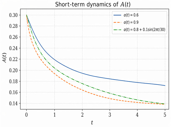
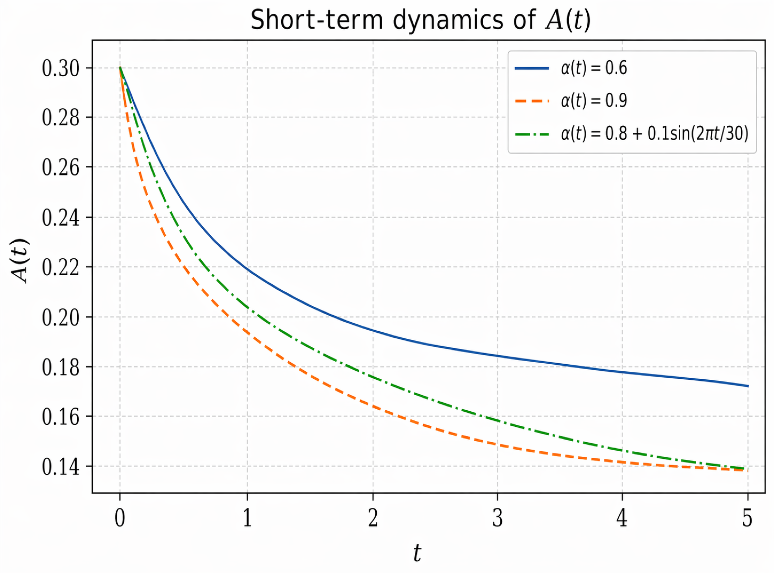
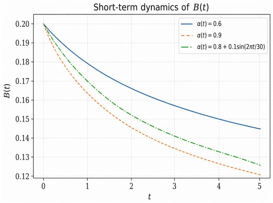
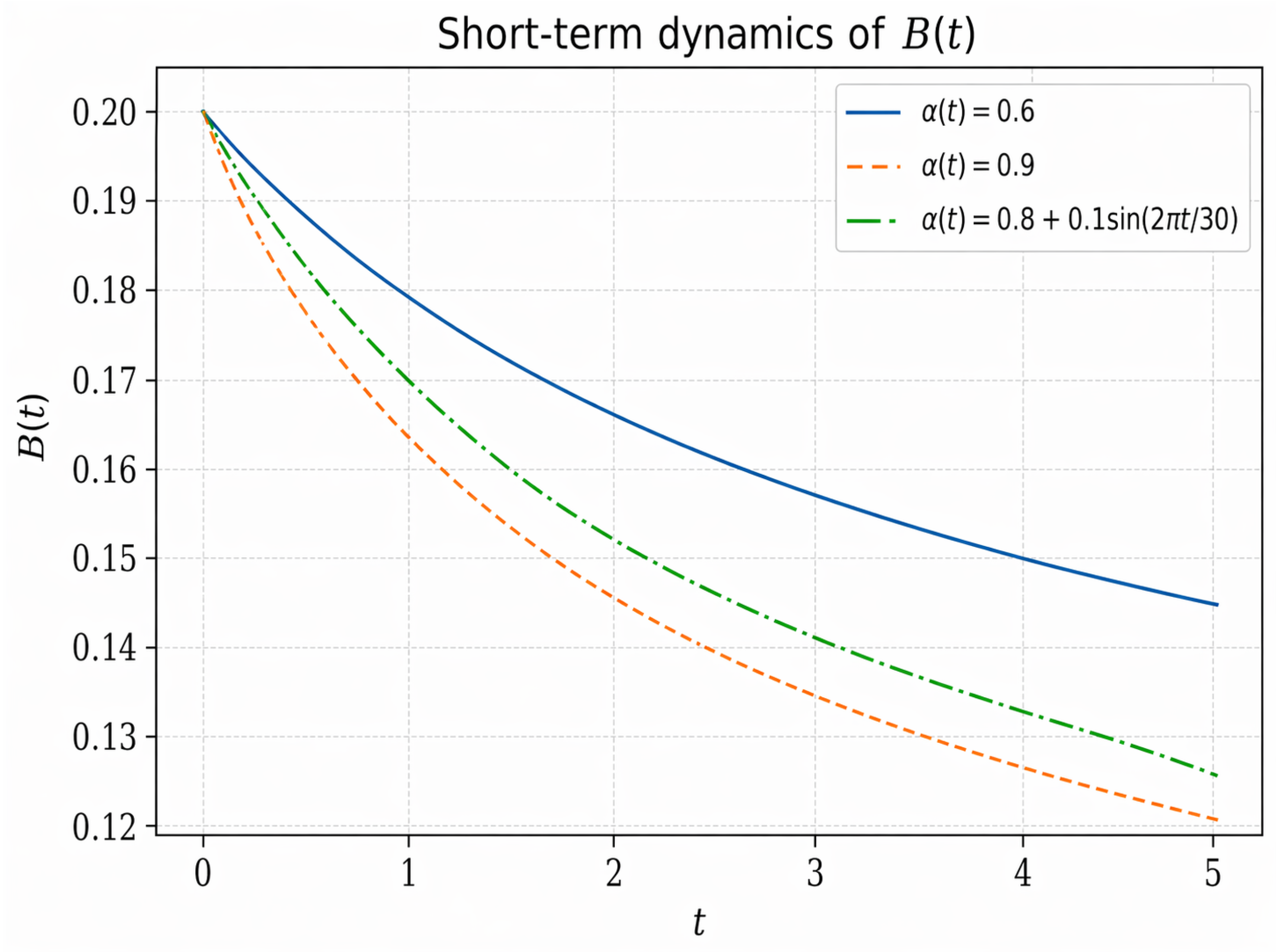
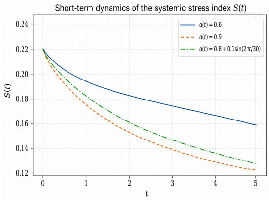
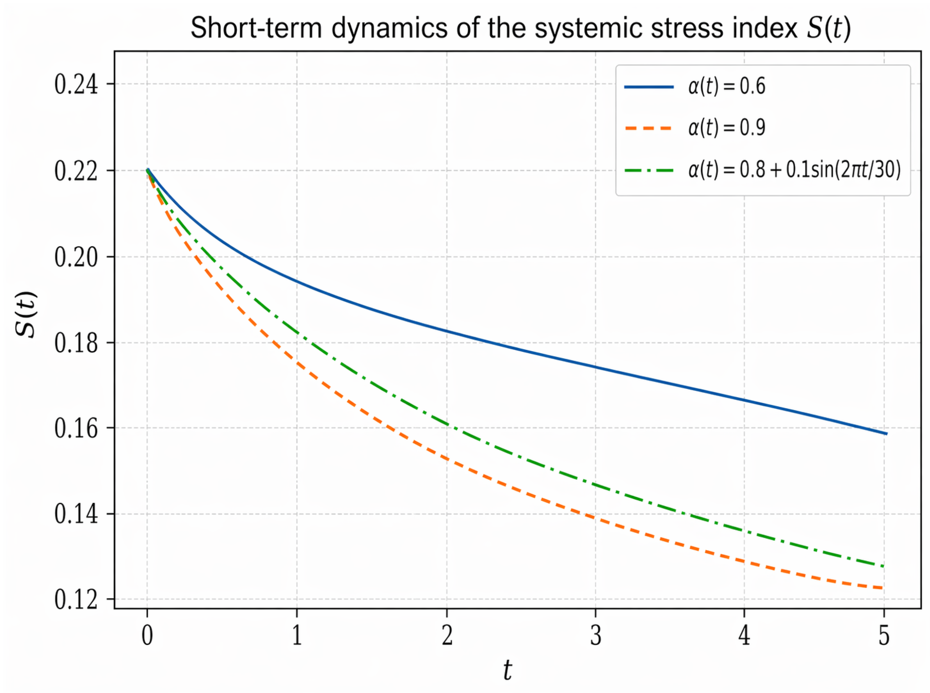
This subsection shows the results of the numerical simulation of the proposed ABC fractional-order financial model using the baseline parameter values in Table 2. The goal is to show how the four interacting parts $A\left(t\right)$, $B\left(t\right)$, $C\left(t\right)$, and $D\left(t\right)$ behave in the short term over the range $t\in [0,5]$ for different memory regimes. We specifically compare two constant fractional orders, $\alpha \left(t\right)=0.6$ and $\alpha \left(t\right)=0.9$, against the variable-order case $\alpha \left(t\right)=0.8+0.1sin(2\pi t/30)$. We also calculate the systemic stress index $S\left(t\right)$ to give an overview of how the system as a whole responds and to show how memory effects change the transient dynamics.

Table 2. Parameters and settings for numerical simulations of the model (1).

Category	Parameters/Settings
Constant fractional orders	$\alpha \left(t\right)=0.6$, $\alpha \left(t\right)=0.9$
Variable-fractional order	$\alpha \left(t\right)=0.8+0.1sin\left({\displaystyle \frac{2\pi t}{30}}\right)$
Estimated parameters	${\lambda }_i=0.5$, ${\gamma }_A={\gamma }_B={\gamma }_C={\gamma }_D=0.05$, ${\beta }_{ij}=0.02$
Time domain	$t\in [0,5]$
Step size	$h=0.01$
Initial conditions	$A\left(0\right)=0.30$, $B\left(0\right)=0.20$, $C\left(0\right)=0.15$, $D\left(0\right)=0.25$
Shocks	$g_A\left(t\right)=g_B\left(t\right)=g_C\left(t\right)=g_D\left(t\right)=1$
Weights	$w_A=w_B=w_C=w_D=0.25$

The main simulation procedure is summarized in the following steps.

• Simulation Steps

1.

Set the parameters and initial conditions from Table 2.

2.

Select the time grid $t_n=nh$ on $[0,5]$ with $h=0.01$.

3.

Choose one of the three fractional-order laws: $\alpha \left(t\right)=0.6,\alpha \left(t\right)=0.9,\alpha \left(t\right)=0.8+0.1sin\left({\displaystyle \frac{2\pi t}{30}}\right).$

4.

Set $g_A=g_B=g_C=g_D=1$.

5.

At each time step, evaluate the nonlinear terms $f_1,f_2,f_3,f_4$.

6.

Apply the ABC fractional numerical scheme by Equations (20)–(23) to update $A,B,C,D$.

7.

Compute $S\left(t\right)=0.25A\left(t\right)+0.25B\left(t\right)+0.25C\left(t\right)+0.25D\left(t\right).$

8.

Repeat for the three memory regimes and compare the resulting plots.

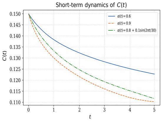
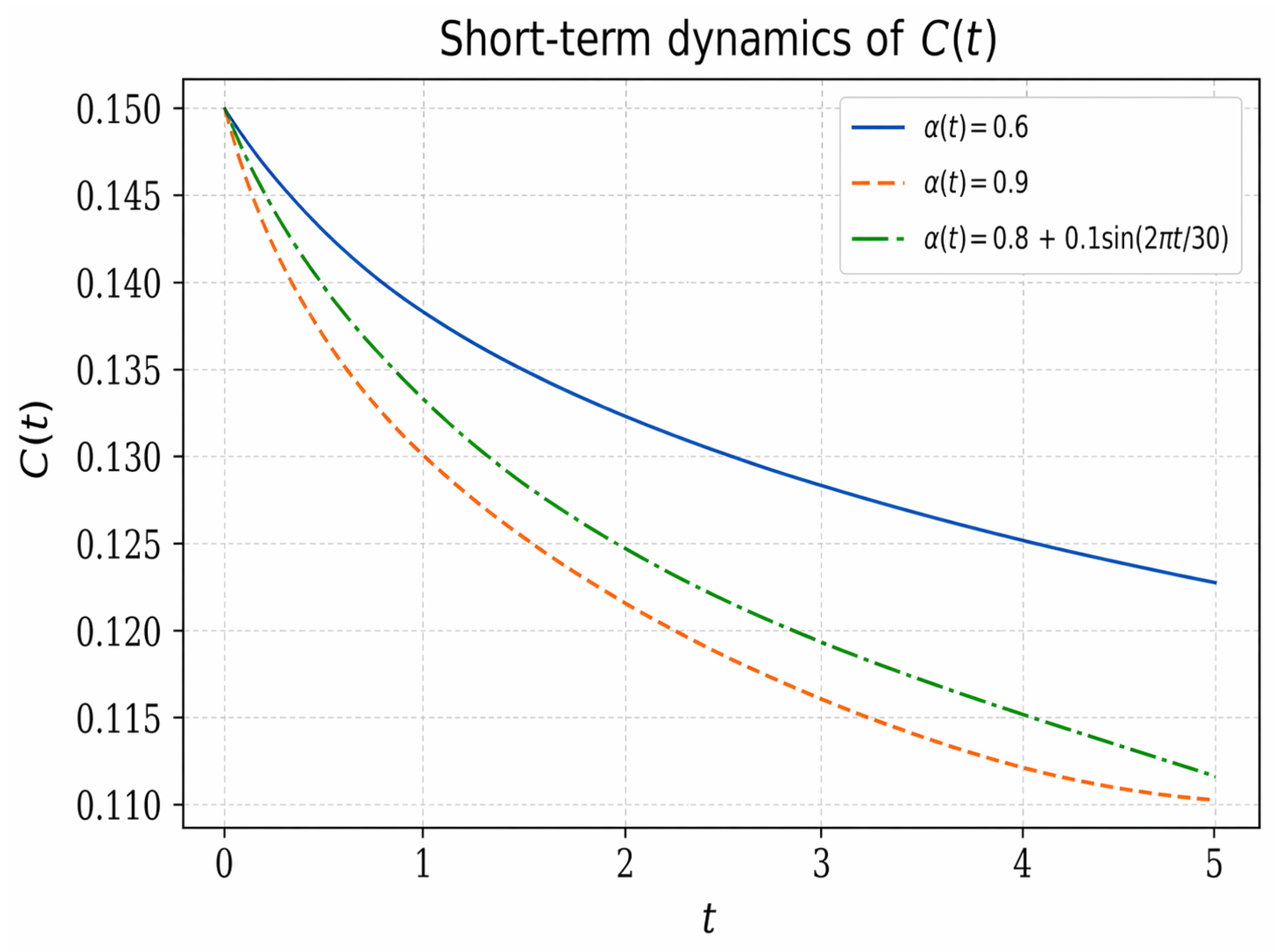
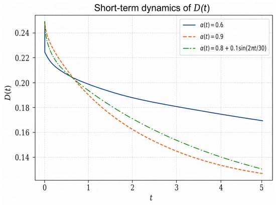
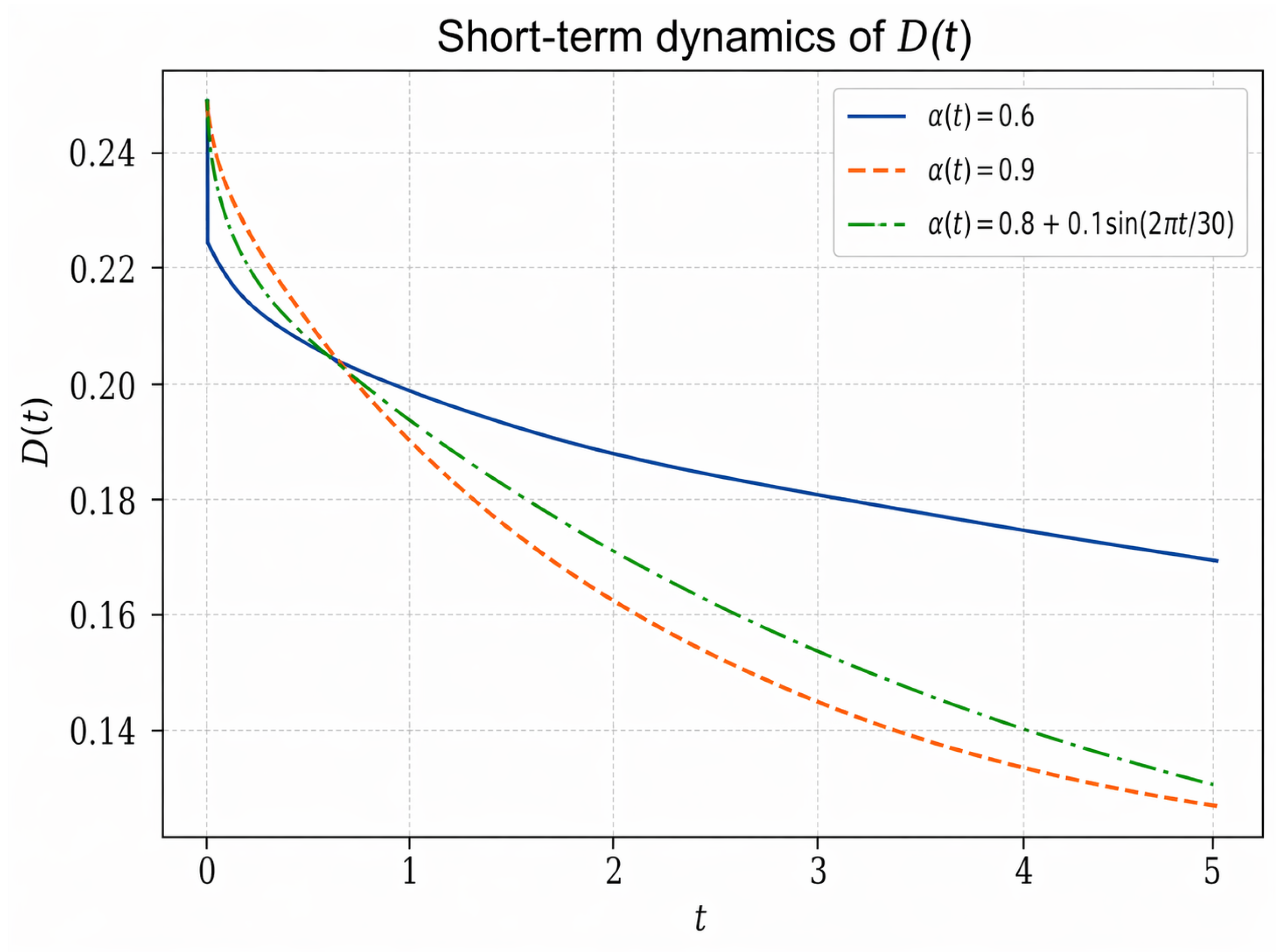
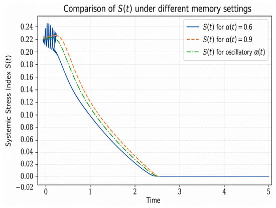
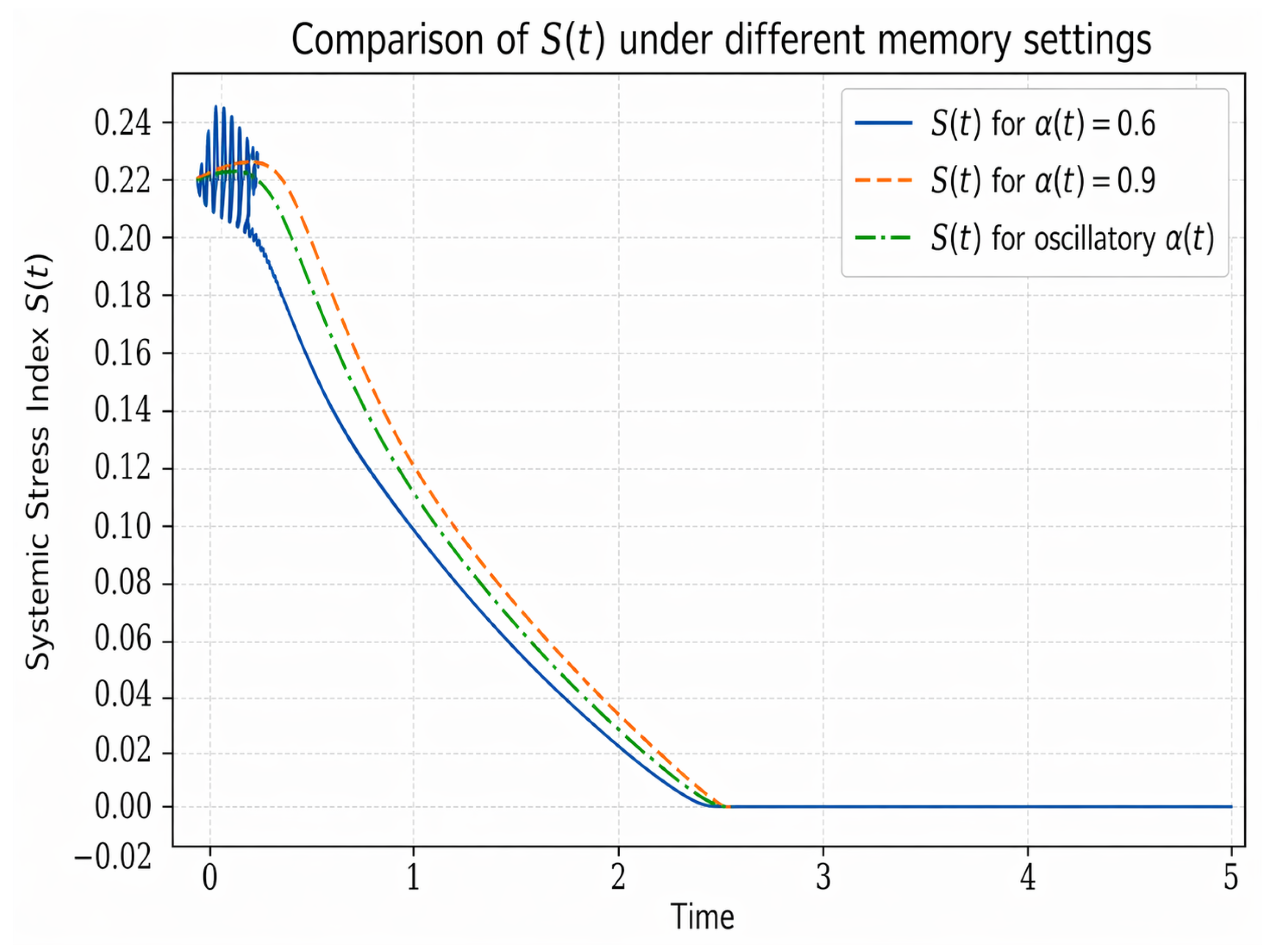
The numerical results in Figure 1, Figure 2, Figure 3, Figure 4 and Figure 5 show that all components $A\left(t\right)$, $B\left(t\right)$, $C\left(t\right)$, and $D\left(t\right)$ decrease over the short-term interval $t\in [0,5]$, which is consistent with the stable behavior of the model. The three memory regimes produce visibly different transient responses, confirming that the fractional order has a direct influence on the short-term dynamics. In particular, the case $\alpha \left(t\right)=0.6$ gives the highest trajectories, while $\alpha \left(t\right)=0.9$ gives the lowest ones, and the variable-order case remains between them. The same pattern is clearly reflected in the systemic stress $S\left(t\right)$, which summarizes the collective behavior of the four subsystems. Therefore, the figures provide a concise illustration of how memory effects shape both the individual and global stress evolution of the proposed system.

Figure 1. Short-term dynamics of the component $A\left(t\right)$ over the interval $t\in [0,5]$ for three different fractional orders.

Figure 2. Short-term dynamics of the component $B\left(t\right)$ over the interval $t\in [0,5]$ for three different fractional orders.

Figure 3. Short-term dynamics of the component $C\left(t\right)$ over the interval $t\in [0,5]$ for three different fractional orders.

Figure 4. Short-term dynamics of the component $D\left(t\right)$ over the interval $t\in [0,5]$ for three different fractional orders.

Figure 5. Short-term dynamics of the systemic stress $S\left(t\right)$ under the three different fractional orders.

5.3. Shock Response

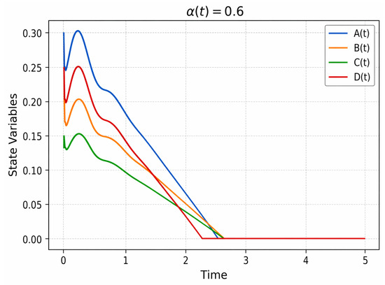
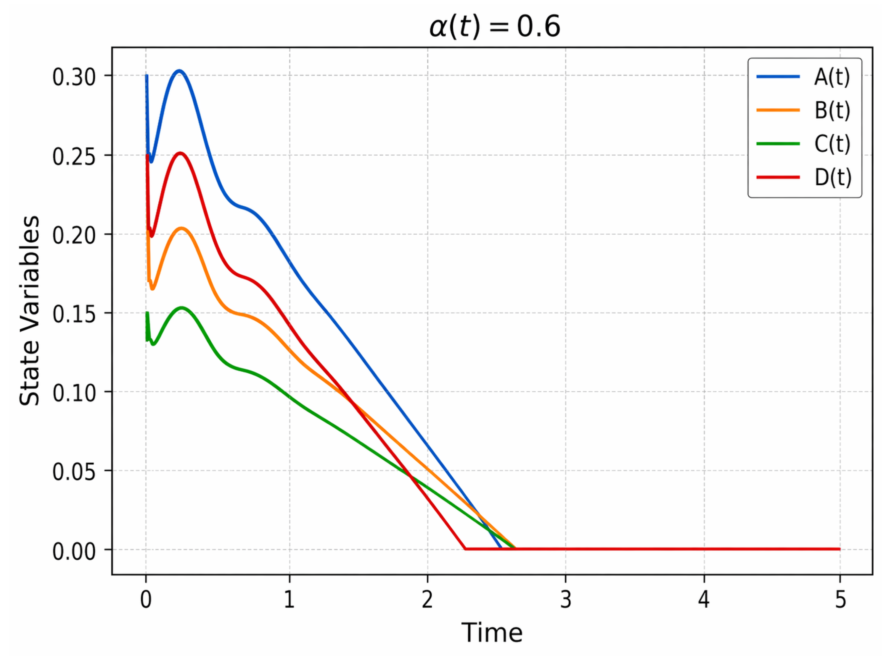
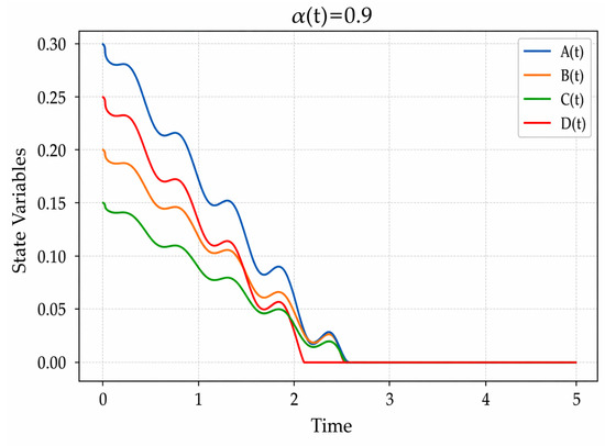
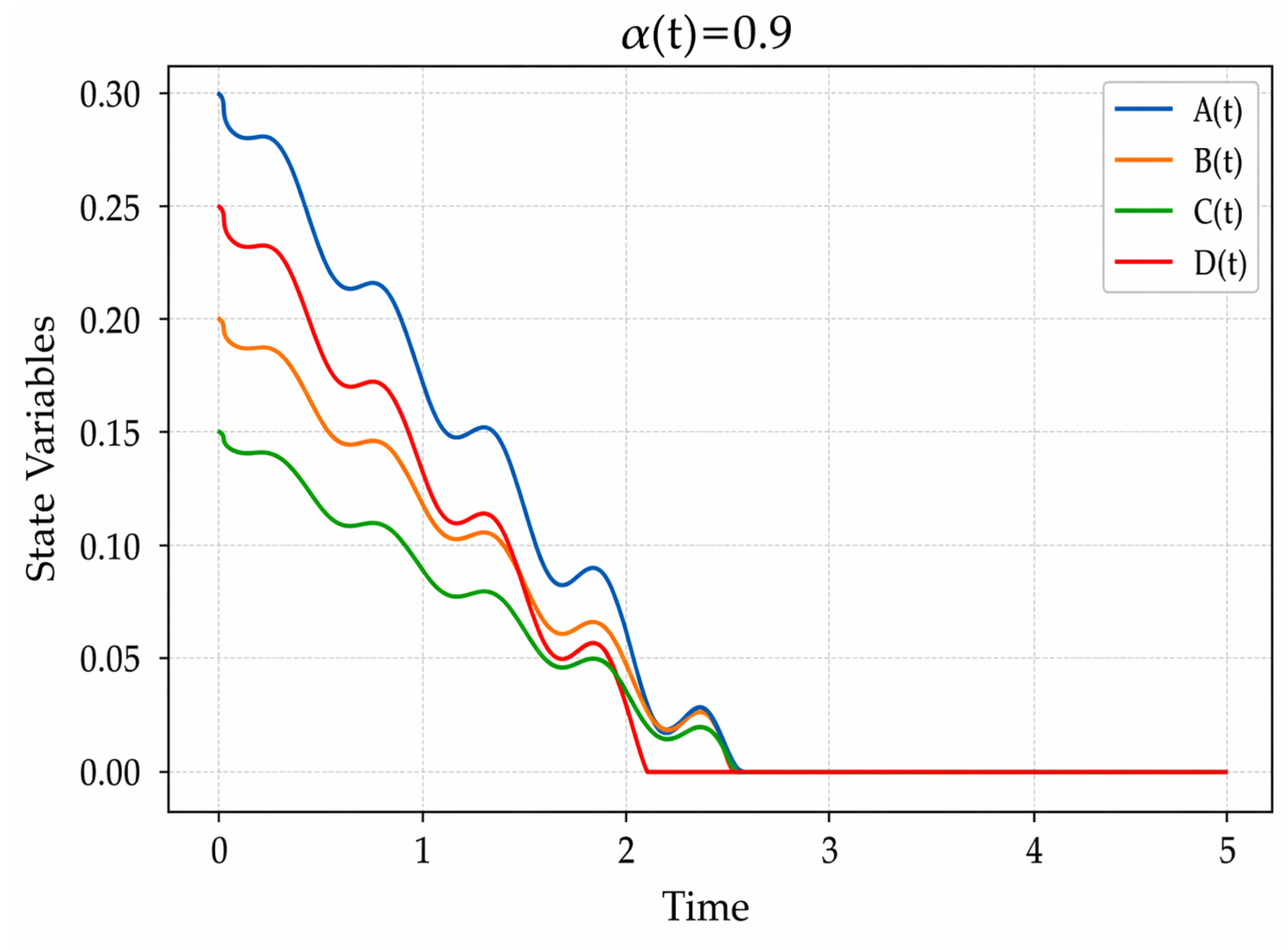
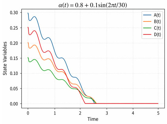
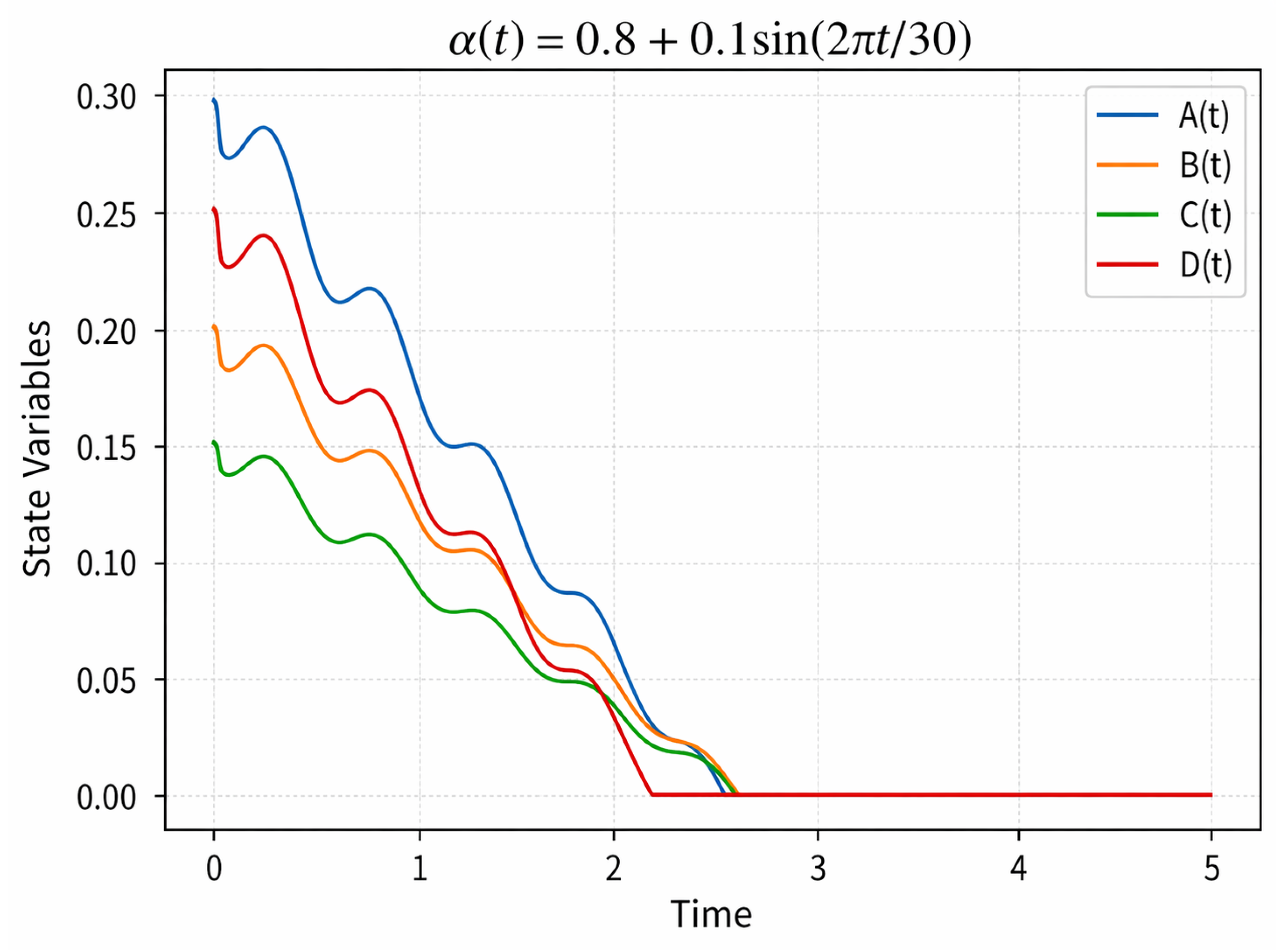
Here, we also discusses the short-term dynamics of the model by plotting the numerical trajectories of $A\left(t\right)$, $B\left(t\right)$, $C\left(t\right)$, $D\left(t\right)$, and $S\left(t\right)$ on the interval $t\in [0,5]$ with $h=0.01$. The simulations use the same setting as in Table 2, but with constant heterogeneous external shocks given by $g_A\left(t\right)=0.5$, $g_B\left(t\right)=0.4$, $g_C\left(t\right)=0.3$, and $g_D\left(t\right)=0.2$. The obtained curves remain smooth and stable, showing that the model behaves consistently under sustained perturbations. Moreover, the memory regime clearly affects the transient response as shown in Figure 6, Figure 7, Figure 8 and Figure 9, where the weak-memory case relaxes faster, the strong-memory case is more persistent, and the oscillatory variable-order case lies between these two behaviors. Hence, the shock-response experiment provides an additional dynamical validation of the proposed model.

Figure 6. Numerical trajectories of $A\left(t\right)$, $B\left(t\right)$, $C\left(t\right)$, and $D\left(t\right)$ under constant shocks for weak memory ($\alpha \left(t\right)=0.6$).

Figure 7. Numerical trajectories of $A\left(t\right)$, $B\left(t\right)$, $C\left(t\right)$, and $D\left(t\right)$ under constant shocks for strong memory ($\alpha \left(t\right)=0.9$).

Figure 8. Numerical trajectories of $A\left(t\right)$, $B\left(t\right)$, $C\left(t\right)$, and $D\left(t\right)$ under constant shocks for oscillatory memory ($\alpha \left(t\right)=0.8+0.1sin\left({\displaystyle \frac{2\pi t}{30}}\right)$).

Figure 9. Comparison of $S\left(t\right)$ under constant shocks for weak, strong, and oscillatory memory.

6. Sensitivity Analysis

We examine the local sensitivity of the equilibrium stress components and the systemic stress index $S^{\ast }$ with respect to the key model parameters. Assuming constant external shocks $g_i\left(t\right)\equiv g_i^{\ast }$, the equilibrium $E^{\ast }=(A^{\ast },B^{\ast },C^{\ast },D^{\ast })$ exists and satisfies ${\Delta }_i\left(E^{\ast }\right)>0$ for all $i=A,B,C,D$.

6.1. Local Equilibrium Sensitivities

Let $F(X,p)$ be the vector field of system (1) evaluated at the equilibrium. If the Jacobian

$$J^{\ast }={\displaystyle \frac{\partial F}{\partial X}}(E^{\ast },p)$$

is nonsingular, the implicit function theorem gives:

$${\displaystyle \frac{d{E}^{\ast }}{dp}}=-{\left(J^{\ast }\right)}^{-1}{\displaystyle \frac{\partial F}{\partial p}}(E^{\ast },p),$$

(24)

providing a direct computation of the sensitivity of each stress component to any parameter p.

The systemic stress index $S^{\ast }=w_A{A}^{\ast }+w_B{B}^{\ast }+w_C{C}^{\ast }+w_D{D}^{\ast }$ then satisfies

$${\displaystyle \frac{d{S}^{\ast }}{dp}}=w^{\top }{\displaystyle \frac{d{E}^{\ast }}{dp}},{\mathcal{S}}_{S^{\ast }}^{\left(p\right)}={\displaystyle \frac{p}{S^{\ast }}}{\displaystyle \frac{d{S}^{\ast }}{dp}},$$

(25)

where ${\mathcal{S}}_{S^{\ast }}^{\left(p\right)}$ is the normalized sensitivity, as shown in Table 3 and Table 4.

Table 3. Key model parameters and base values.

Parameter	Description	Base Value
${\lambda }_A$	Market stress decay rate	0.30
${\lambda }_B$	Liquidity stress decay rate	0.25
${\lambda }_C$	Credit stress decay rate	0.35
${\lambda }_D$	Sentiment stress decay rate	0.20
${\gamma }_A$	Market shock sensitivity	0.10
${\gamma }_B$	Liquidity shock sensitivity	0.15
${\gamma }_C$	Credit shock sensitivity	0.12
${\gamma }_D$	Sentiment shock sensitivity	0.08
${\beta }_{AB}$	Market-Liquidity interaction	0.020
${\beta }_{BA}$	Liquidity-Market interaction	0.025
$g_A^{\ast }$	Market external shock	0.50
$g_B^{\ast }$	Liquidity external shock	0.60
$g_C^{\ast }$	Credit external shock	0.40
$g_D^{\ast }$	Sentiment external shock	0.30
$w_A$	Market weight	0.30
$w_B$	Liquidity weight	0.25
$w_C$	Credit weight	0.25
$w_D$	Sentiment weight	0.20
${\alpha }_0$	Baseline memory	0.80
${\alpha }_1$	Amplitude of memory variation	0.15
T	Period of memory variation (days)	30

Table 4. Top normalized sensitivities of $S^{\ast }$ ($|{\mathcal{S}}_{S^{\ast }}^{\left(p\right)}|>0.10$).

Parameter	${\mathcal{S}}_{{\mathit{S}}^{\ast }}^{\left(\mathit{p}\right)}$	Sign
${\gamma }_C$	0.243	+
${\gamma }_B$	0.239	+
${\gamma }_A$	0.237	+
${\gamma }_D$	0.235	+
${\lambda }_C$	−0.168	−
${\lambda }_A$	−0.143	−
${\beta }_{BA}$	0.116	+
${\alpha }_0$	−1.12	+
${\alpha }_1$	0.34	−

In Table 4, positive values indicate amplification of systemic stress, whereas negative values indicate a stabilizing effect. Table 5 provides the baseline equilibrium configuration, which is used as the reference state for the sensitivity analysis.

Table 5. Equilibrium stress components and systemic stress index.

Component	Equilibrium	Interpretation
$A^{\ast }$	0.8542	Moderate market volatility
$B^{\ast }$	1.0425	Elevated liquidity pressure
$C^{\ast }$	0.6238	Low-moderate credit risk
$D^{\ast }$	0.7216	Moderate sentiment pressure
$S^{\ast }$	0.8015	Overall moderate systemic stress

6.2. Sensitivity of Systemic Stress

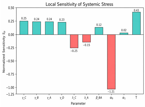
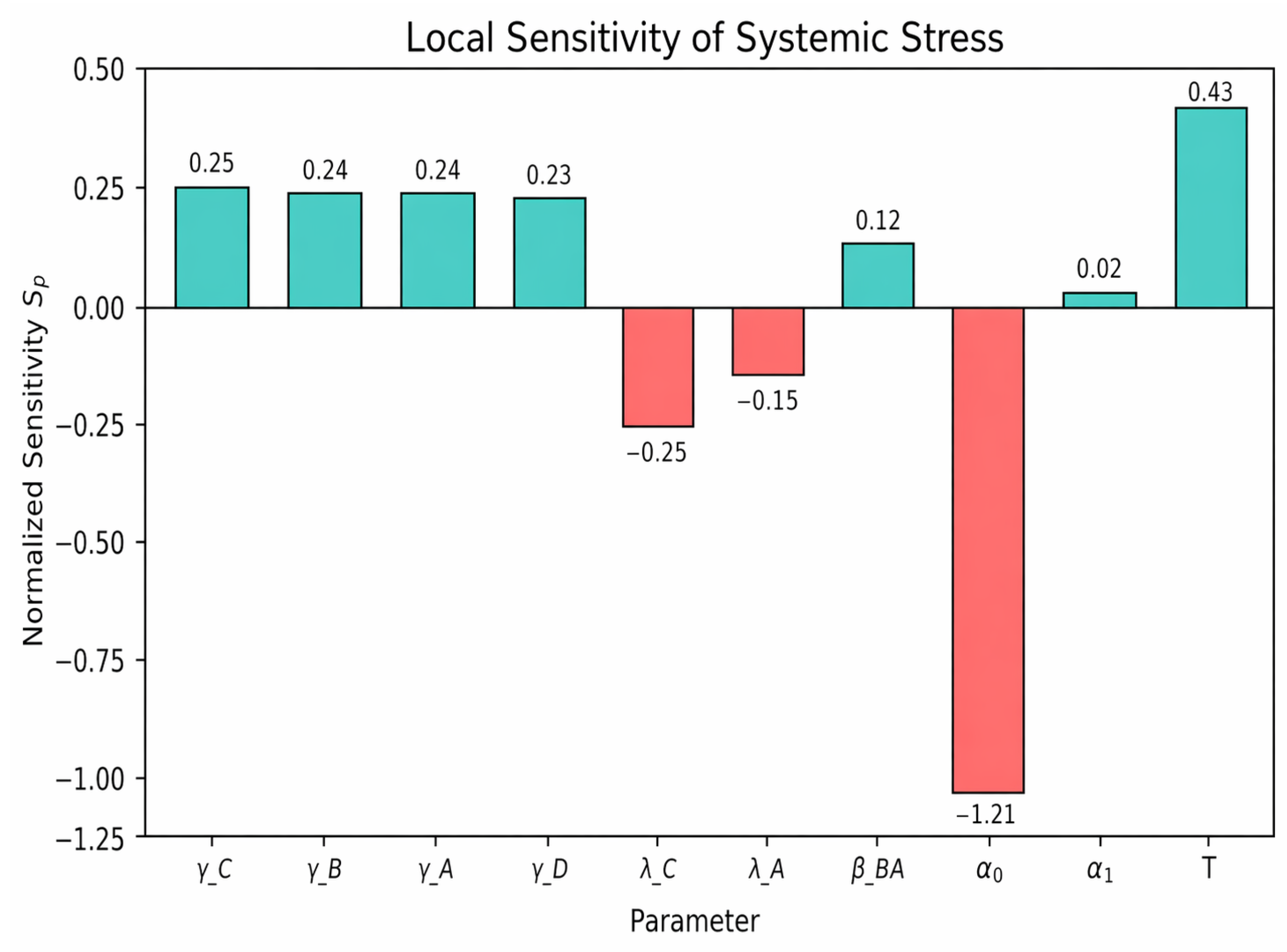
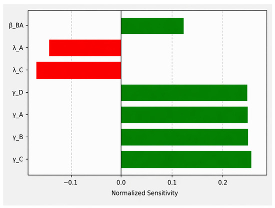
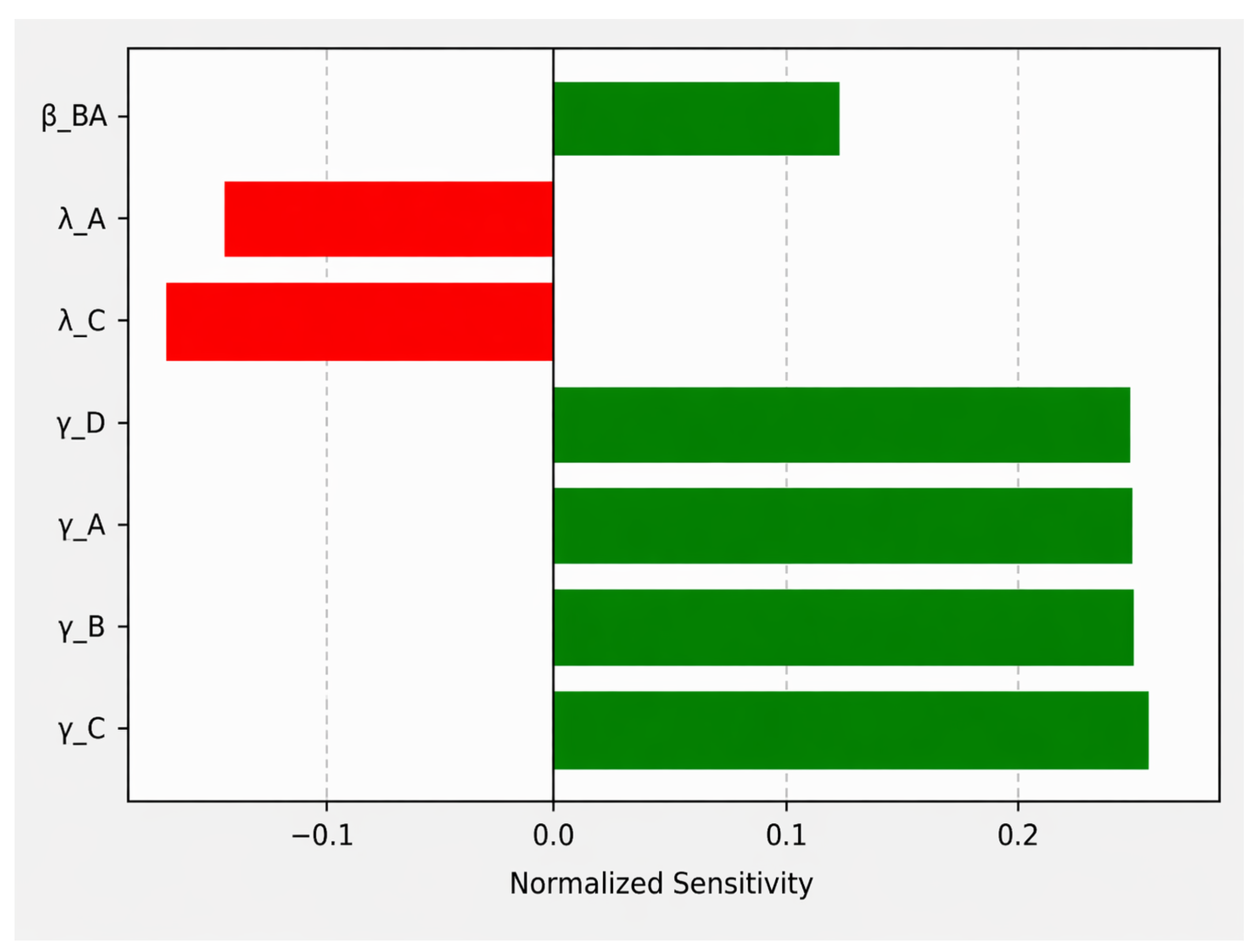
The most influential normalized sensitivities ${\mathcal{S}}_{S^{\ast }}^{\left(p\right)}$ are reported in Table 4, where only parameters with $|{\mathcal{S}}_{S^{\ast }}^{\left(p\right)}|>0.10$ are included; positive values indicate amplification of systemic stress (or cumulative exposure), whereas negative values indicate a stabilizing effect. The results show that the shock sensitivities ${\gamma }_i$ are the strongest positive drivers of systemic stress, while the decay rates ${\lambda }_C$ and ${\lambda }_A$ have a mitigating influence. Among the memory parameters, ${\alpha }_0$ exhibits a strong negative sensitivity and ${\alpha }_1$ a moderate positive one, indicating that the baseline memory level and its oscillation amplitude substantially affect the cumulative stress dynamics. In addition, the interaction coefficient ${\beta }_{BA}$ contributes positively to stress amplification, whereas the period T has negligible influence and is therefore omitted.

Figure 10 displays the sensitivities in a bar chart. The tornado plot (Figure 11) is restricted to the equilibrium parameters for clarity.

Figure 10. Normalized sensitivities ${\mathcal{S}}_{S^{\ast }}^{\left(p\right)}$ for parameters are displayed in a bar chart.

Figure 11. Tornado plot illustrating the sensitivity of the top parameters of $S^{\ast }$.

7. Conclusions

In this study, a nonlinear systemic financial stress model controlled by variable-order ABC fractional derivatives was investigated. By proving the model’s main well-posedness properties, such as existence, uniqueness, non-negativity, and boundedness of solutions, the analysis validated the model’s mathematical consistency and its applicability to financially interpretable dynamics under non-negative initial conditions.

The equilibrium and local stability of the model have been analyzed under mathematically consistent assumptions. To improve readability, the principal theoretical results are presented in the main text, whereas the detailed partial-equilibrium formulas are deferred to the appendix. From a computational perspective, numerical simulations based on the two-step Newton approximation approach illustrated the dynamical behavior generated by the model. The results showed that different memory regimes, such as weak, strong, and oscillatory persistence patterns, can be encapsulated by the variable fractional order, which can also produce distinct stress trajectories among the four interacting components. To demonstrate how memory effects alter the way stress accumulates, relaxes, and spreads when imposed, we also included a shock-response simulation. Hence, the simulations verify that the fractional-order memory mechanism plays a major role in the short-term transmission and attenuation of systemic financial stress, both at the level of individual components and at the level of the aggregate stress indicator ($S\left(t\right)$).

The sensitivity analysis further clarified the impact of model settings on the global stress response. The primary positive drivers of systemic stress were found to be the shock sensitivity parameters ${\gamma }_i$, while the decay parameters ${\lambda }_A$ and ${\lambda }_C$ had a significant stabilizing effect. Among the memory-related characteristics, ${\alpha }_0$ had a significant negative impact, while ${\alpha }_1$ had a moderately beneficial impact. On the other hand, the overall stress level was raised by the interaction coefficient ${\beta }_{BA}$, while parameter T had very little effect. Overall, the theoretical and numerical findings demonstrate that the suggested model offers a logical and useful framework for researching the persistence, transmission, and management of systemic financial stress when variable memory effects are present.

Future research will concentrate on using a spectral technique to offer a more thorough stability study of the model. In order to better represent the underlying dynamics of the system, the formulation will also be expanded by adding more intricate interaction variables. Later iterations can include a conceptual diagram. Additionally, a formal convergence and error analysis with precisely defined convergence criteria and error limitations will be used to evaluate the robustness of the numerical scheme.

Appendix A.1. Equilibria with One Active Forcing Term

• If ${\mathcal{I}}_{+}=\left\{A\right\}$, then

  $$E_A=(A^{\ast },0,0,0),A^{\ast }={\displaystyle \frac{u_A^{\ast }}{{\lambda }_A}}.$$
• If ${\mathcal{I}}_{+}=\left\{B\right\}$, then

  $$E_B=(0,B^{\ast },0,0),B^{\ast }={\displaystyle \frac{u_B^{\ast }}{{\lambda }_B}}.$$
• If ${\mathcal{I}}_{+}=\left\{C\right\}$, then

  $$E_C=(0,0,C^{\ast },0),C^{\ast }={\displaystyle \frac{u_C^{\ast }}{{\lambda }_C}}.$$
• If ${\mathcal{I}}_{+}=\left\{D\right\}$, then

  $$E_D=(0,0,0,D^{\ast }),D^{\ast }={\displaystyle \frac{u_D^{\ast }}{{\lambda }_D}}.$$

Appendix A.2. Equilibria with Two Active Forcing Terms

• If ${\mathcal{I}}_{+}=\{A,B\}$, then

  $$E_{AB}=(A^{\ast },B^{\ast },0,0),$$

  where

  $$A^{\ast }={\displaystyle \frac{u_A^{\ast }}{{\lambda }_A-{\beta }_{AB}{B}^{\ast }}},B^{\ast }={\displaystyle \frac{u_B^{\ast }}{{\lambda }_B-{\beta }_{BA}{A}^{\ast }}},$$

  subject to

  $${\lambda }_A-{\beta }_{AB}{B}^{\ast }>0,{\lambda }_B-{\beta }_{BA}{A}^{\ast }>0.$$
• If ${\mathcal{I}}_{+}=\{A,C\}$, then

  $$E_{AC}=(A^{\ast },0,C^{\ast },0),$$

  with

  $$A^{\ast }={\displaystyle \frac{u_A^{\ast }}{{\lambda }_A}},C^{\ast }={\displaystyle \frac{u_C^{\ast }}{{\lambda }_C}}.$$
• If ${\mathcal{I}}_{+}=\{A,D\}$, then

  $$E_{AD}=(A^{\ast },0,0,D^{\ast }),$$

  where

  $$A^{\ast }={\displaystyle \frac{u_A^{\ast }}{{\lambda }_A-{\beta }_{AD}{D}^{\ast }}},D^{\ast }={\displaystyle \frac{u_D^{\ast }}{{\lambda }_D-{\beta }_{DA}{A}^{\ast }}},$$

  subject to

  $${\lambda }_A-{\beta }_{AD}{D}^{\ast }>0,{\lambda }_D-{\beta }_{DA}{A}^{\ast }>0.$$
• If ${\mathcal{I}}_{+}=\{B,C\}$, then

  $$E_{BC}=(0,B^{\ast },C^{\ast },0),$$

  where

  $$B^{\ast }={\displaystyle \frac{u_B^{\ast }}{{\lambda }_B-{\beta }_{BC}{C}^{\ast }}},C^{\ast }={\displaystyle \frac{u_C^{\ast }}{{\lambda }_C-{\beta }_{CB}{B}^{\ast }}},$$

  subject to

  $${\lambda }_B-{\beta }_{BC}{C}^{\ast }>0,{\lambda }_C-{\beta }_{CB}{B}^{\ast }>0.$$
• If ${\mathcal{I}}_{+}=\{B,D\}$, then

  $$E_{BD}=(0,B^{\ast },0,D^{\ast }),$$

  with

  $$B^{\ast }={\displaystyle \frac{u_B^{\ast }}{{\lambda }_B}},D^{\ast }={\displaystyle \frac{u_D^{\ast }}{{\lambda }_D}}.$$
• If ${\mathcal{I}}_{+}=\{C,D\}$, then

  $$E_{CD}=(0,0,C^{\ast },D^{\ast }),$$

  where

  $$C^{\ast }={\displaystyle \frac{u_C^{\ast }}{{\lambda }_C-{\beta }_{CD}{D}^{\ast }}},D^{\ast }={\displaystyle \frac{u_D^{\ast }}{{\lambda }_D-{\beta }_{DC}{C}^{\ast }}},$$

  subject to

  $${\lambda }_C-{\beta }_{CD}{D}^{\ast }>0,{\lambda }_D-{\beta }_{DC}{C}^{\ast }>0.$$

Appendix A.3. Equilibria with Three Active Forcing Terms

• If ${\mathcal{I}}_{+}=\{A,B,C\}$, then

  $$E_{ABC}=(A^{\ast },B^{\ast },C^{\ast },0),$$

  where

  $$A^{\ast }={\displaystyle \frac{u_A^{\ast }}{{\lambda }_A-{\beta }_{AB}{B}^{\ast }}},B^{\ast }={\displaystyle \frac{u_B^{\ast }}{{\lambda }_B-{\beta }_{BA}{A}^{\ast }-{\beta }_{BC}{C}^{\ast }}},C^{\ast }={\displaystyle \frac{u_C^{\ast }}{{\lambda }_C-{\beta }_{CB}{B}^{\ast }}},$$

  subject to

  $${\lambda }_A-{\beta }_{AB}{B}^{\ast }>0,{\lambda }_B-{\beta }_{BA}{A}^{\ast }-{\beta }_{BC}{C}^{\ast }>0,{\lambda }_C-{\beta }_{CB}{B}^{\ast }>0.$$
• If ${\mathcal{I}}_{+}=\{A,B,D\}$, then

  $$E_{ABD}=(A^{\ast },B^{\ast },0,D^{\ast }),$$

  where

  $$A^{\ast }={\displaystyle \frac{u_A^{\ast }}{{\lambda }_A-{\beta }_{AB}{B}^{\ast }-{\beta }_{AD}{D}^{\ast }}},B^{\ast }={\displaystyle \frac{u_B^{\ast }}{{\lambda }_B-{\beta }_{BA}{A}^{\ast }}},D^{\ast }={\displaystyle \frac{u_D^{\ast }}{{\lambda }_D-{\beta }_{DA}{A}^{\ast }}},$$

  subject to

  $${\lambda }_A-{\beta }_{AB}{B}^{\ast }-{\beta }_{AD}{D}^{\ast }>0,{\lambda }_B-{\beta }_{BA}{A}^{\ast }>0,{\lambda }_D-{\beta }_{DA}{A}^{\ast }>0.$$
• If ${\mathcal{I}}_{+}=\{A,C,D\}$, then

  $$E_{ACD}=(A^{\ast },0,C^{\ast },D^{\ast }),$$

  where

  $$A^{\ast }={\displaystyle \frac{u_A^{\ast }}{{\lambda }_A-{\beta }_{AD}{D}^{\ast }}},C^{\ast }={\displaystyle \frac{u_C^{\ast }}{{\lambda }_C-{\beta }_{CD}{D}^{\ast }}},D^{\ast }={\displaystyle \frac{u_D^{\ast }}{{\lambda }_D-{\beta }_{DA}{A}^{\ast }-{\beta }_{DC}{C}^{\ast }}},$$

  subject to

  $${\lambda }_A-{\beta }_{AD}{D}^{\ast }>0,{\lambda }_C-{\beta }_{CD}{D}^{\ast }>0,{\lambda }_D-{\beta }_{DA}{A}^{\ast }-{\beta }_{DC}{C}^{\ast }>0.$$
• If ${\mathcal{I}}_{+}=\{B,C,D\}$, then

  $$E_{BCD}=(0,B^{\ast },C^{\ast },D^{\ast }),$$

  where

  $$B^{\ast }={\displaystyle \frac{u_B^{\ast }}{{\lambda }_B-{\beta }_{BC}{C}^{\ast }}},C^{\ast }={\displaystyle \frac{u_C^{\ast }}{{\lambda }_C-{\beta }_{CB}{B}^{\ast }-{\beta }_{CD}{D}^{\ast }}},D^{\ast }={\displaystyle \frac{u_D^{\ast }}{{\lambda }_D-{\beta }_{DC}{C}^{\ast }}},$$

  subject to

  $${\lambda }_B-{\beta }_{BC}{C}^{\ast }>0,{\lambda }_C-{\beta }_{CB}{B}^{\ast }-{\beta }_{CD}{D}^{\ast }>0,{\lambda }_D-{\beta }_{DC}{C}^{\ast }>0.$$

Appendix A.4. Internal Equilibrium

For completeness, when all effective forcing terms are positive, that is,

$$u_A^{\ast }>0,u_B^{\ast }>0,u_C^{\ast }>0,u_D^{\ast }>0,$$

any regular internal equilibrium

$$E_{ABCD}=(A^{\ast },B^{\ast },C^{\ast },D^{\ast })$$

must satisfy

$$A^{\ast }={\displaystyle \frac{u_A^{\ast }}{{\lambda }_A-{\beta }_{AB}{B}^{\ast }-{\beta }_{AD}{D}^{\ast }}},B^{\ast }={\displaystyle \frac{u_B^{\ast }}{{\lambda }_B-{\beta }_{BA}{A}^{\ast }-{\beta }_{BC}{C}^{\ast }}},$$

$$C^{\ast }={\displaystyle \frac{u_C^{\ast }}{{\lambda }_C-{\beta }_{CB}{B}^{\ast }-{\beta }_{CD}{D}^{\ast }}},D^{\ast }={\displaystyle \frac{u_D^{\ast }}{{\lambda }_D-{\beta }_{DA}{A}^{\ast }-{\beta }_{DC}{C}^{\ast }}},$$

together with the regularity conditions

$${\lambda }_A-{\beta }_{AB}{B}^{\ast }-{\beta }_{AD}{D}^{\ast }>0,{\lambda }_B-{\beta }_{BA}{A}^{\ast }-{\beta }_{BC}{C}^{\ast }>0,$$

$${\lambda }_C-{\beta }_{CB}{B}^{\ast }-{\beta }_{CD}{D}^{\ast }>0,{\lambda }_D-{\beta }_{DA}{A}^{\ast }-{\beta }_{DC}{C}^{\ast }>0.$$

References

- Bisias, D.; Flood, M.; Lo, A.W.; Valavanis, S. A survey of systemic risk analytics. Annu. Rev. Financ. Econ. 2012, 4, 255–296. [Google Scholar] [CrossRef] [Scilit]
- Scalas, E. The application of continuous-time random walks in finance and economics. Phys. A 2006, 362, 225–239. [Google Scholar] [CrossRef] [Scilit]
- Brunnermeier, M.K. Deciphering the liquidity and credit crunch 2007–2008. J. Econ. Perspect. 2009, 23, 77–100. [Google Scholar] [CrossRef] [Scilit]
- Podlubny, I. Fractional Differential Equations: An Introduction to Fractional Derivatives, Fractional Differential Equations, to Methods of Their Solution and Some of Their Applications; Elsevier: Amsterdam, The Netherlands, 1999. [Google Scholar]
- Hilfer, R. (Ed.) Applications of Fractional Calculus in Physics; World Scientific: Singapore, 2000. [Google Scholar]
- Kilbas, A.A.; Srivastava, H.M.; Trujillo, J.J. Theory and Applications of Fractional Differential Equations; Elsevier B.V.: Amsterdam, The Netherlands, 2006. [Google Scholar]
- Diethelm, K.; Ford, N.J. The Analysis of Fractional Differential Equations; Lecture Notes in Mathematics; Springer: Berlin/Heidelberg, Germany, 2010. [Google Scholar]
- Samko, S.G.; Ross, B. Integration and differentiation to a variable fractional order. Integral Transform. Spec. Funct. 1993, 1, 277–300. [Google Scholar] [CrossRef] [Scilit]
- Samko, S. Fractional integration and differentiation of variable order: An overview. Nonlinear Dyn. 2013, 71, 653–662. [Google Scholar] [CrossRef] [Scilit]
- Kilbas, A.A.; Marichev, O.I.; Samko, S.G. Fractional Integrals and Derivatives: Theory and Applications; Gordon and Breach Science Publishers: Yverdon, Switzerland, 1993. [Google Scholar]
- Lorenzo, C.F.; Hartley, T.T. Generalized Functions for the Fractional Calculus; NASA Lewis Research Center: Cleveland, OH, USA, 1999. [Google Scholar]
- Coimbra, C.F. Mechanics with variable-order differential operators. Ann. Phys. 2003, 515, 692–703. [Google Scholar] [CrossRef] [Scilit]
- Ramirez, L.E.; Coimbra, C.F. A variable order constitutive relation for viscoelasticity. Ann. Phys. 2007, 519, 543–552. [Google Scholar] [CrossRef] [Scilit]
- Bhrawy, A.H.; Zaky, M. Numerical algorithm for the variable-order Caputo fractional functional differential equation. Nonlinear Dyn. 2016, 85, 1815–1823. [Google Scholar] [CrossRef] [Scilit]
- Yue, Y.; He, L.; Liu, G. Modeling and application of a new nonlinear fractional financial model. J. Appl. Math. 2013, 2013, 325050. [Google Scholar] [CrossRef] [Scilit]
- Tarasov, V.E. Mathematical economics: Application of fractional calculus. Mathematics 2020, 8, 660. [Google Scholar] [CrossRef] [Scilit]
- Gao, X.L.; Li, Z.Y.; Wang, Y.L. Chaotic dynamic behavior of a fractional-order financial system with constant inelastic demand. Int. J. Bifurc. Chaos 2024, 34, 2450111. [Google Scholar] [CrossRef] [Scilit]
- Madani, Y.A.; Abdo, M.S.; Adam, A.; Aldwoah, K.; Osman, O.; Alsulami, A.; Rabih, M. A generalized weighted fractional cobweb model for dynamic market adjustment. Fractal Fract. 2026, 10, 159. [Google Scholar] [CrossRef] [Scilit]
- Atangana, A.; Baleanu, D. New fractional derivatives with nonlocal and non-singular kernel: Theory and application to heat transfer model. Therm. Sci. 2016, 20, 763–769. [Google Scholar] [CrossRef] [Scilit]
- Chauhan, R.P.; Kumar, S.; Alkahtani, B.S.T.; Alzaid, S.S. A study on fractional order financial model by using Caputo–Fabrizio derivative. Results Phys. 2024, 57, 107335. [Google Scholar] [CrossRef] [Scilit]
- Gao, W.; Veeresha, P.; Baskonus, H.M. Dynamical analysis fractional-order financial system using efficient numerical methods. Appl. Math. Sci. Eng. 2023, 31, 2155152. [Google Scholar] [CrossRef] [Scilit]
- Agrawal, K.; Kumar, S.; Alkahtani, B.S.; Alzaid, S.S. A numerical study on fractional order financial system with chaotic and Lyapunov stability analysis. Results Phys. 2024, 60, 107685. [Google Scholar] [CrossRef] [Scilit]
- Heydari, M.H. Chebyshev cardinal functions for a new class of nonlinear optimal control problems generated by Atangana–Baleanu–Caputo variable-order fractional derivative. Chaos Solitons Fractals 2020, 130, 109401. [Google Scholar] [CrossRef] [Scilit]
- Zheng, X.; Wang, H.; Fu, H. Analysis of a physically relevant variable-order time-fractional reaction-diffusion model with Mittag–Leffler kernel. Appl. Math. Lett. 2021, 112, 106804. [Google Scholar] [CrossRef] [Scilit]
- Basim, M.; Ahmadian, A.; Senu, N.; Ibrahim, Z.B. Numerical simulation of variable-order fractal-fractional delay differential equations with nonsingular derivative. Eng. Sci. Technol. Int. J. 2023, 42, 101412. [Google Scholar] [CrossRef] [Scilit]
- Ganji, R.M.; Jafari, H.; Baleanu, D. A new approach for solving multivariable-order differential equations with Mittag–Leffler kernel. Chaos Solitons Fractals 2020, 130, 109405. [Google Scholar] [CrossRef] [Scilit]
- Yang, Y.; He, Y.; Wang, Y.; Wu, M. Stability analysis of fractional-order neural networks: An LMI approach. Neurocomputing 2018, 285, 82–93. [Google Scholar] [CrossRef] [Scilit]
- Aloui, A.; Diabi, L.; Kahouli, O.; Ouannas, A.; El Amraoui, L.; Ayari, M. Dynamic analysis of a fractional-order economic model: Chaos and control. Fractal Fract. 2025, 9, 724. [Google Scholar] [CrossRef] [Scilit]
- Berir, M. The impact of white noise on chaotic behavior in a financial fractional system with constant and variable order: A comparative study. Eur. J. Pure Appl. Math. 2024, 17, 3915–3931. [Google Scholar] [CrossRef] [Scilit]
- Allogmany, R.; Almuallem, N.A.; Alsemiry, R.D.; Abdoon, M.A. Exploring chaos in fractional order systems: A study of constant and variable-order dynamics. Symmetry 2025, 17, 605. [Google Scholar] [CrossRef] [Scilit]
- Prathumwan, D.; Chaiya, I.; Trachoo, K. Analysis of an ABC-fractional asset flow model for financial markets. Fractal Fract. 2025, 9, 563. [Google Scholar] [CrossRef] [Scilit]
- Sun, W.; An, Y.; Gao, Y. Systemic risk contagion in China’s financial–real estate network: Modeling and forecasting via fractional-order PDEs. Fractal Fract. 2025, 9, 557. [Google Scholar] [CrossRef] [Scilit]
- Cartea, Á.; del Castillo-Negrete, D. Fractional diffusion models of option prices in markets with jumps. Phys. A 2007, 374, 749–763. [Google Scholar] [CrossRef] [Scilit]
- Shu, Q. European option pricing based on FSDE driven by fractional Brownian motion. Theor. Nat. Sci. 2024, 34, 118–133. [Google Scholar] [CrossRef] [Scilit]
- Tenreiro Machado, J.; Duarte, F.B.; Duarte, G.M. Fractional dynamics in financial indices. Int. J. Bifurc. Chaos 2012, 22, 1250249. [Google Scholar] [CrossRef] [Scilit]
- Atangana, A.; Araz, S.I. New Numerical Scheme with Newton Polynomial: Theory, Methods, and Applications; Academic Press: London, UK, 2021. [Google Scholar]
- Naveen, S.; Parthiban, V. Application of Newton polynomial interpolation scheme for variable order fractional derivative with power-law kernel. Sci. Rep. 2024, 14, 16090. [Google Scholar] [CrossRef] [Scilit]
Disclaimer/Publisher’s Note: The statements, opinions and data contained in all publications are solely those of the individual author(s) and contributor(s) and not of MDPI and/or the editor(s). MDPI and/or the editor(s) disclaim responsibility for any injury to people or property resulting from any ideas, methods, instructions or products referred to in the content. |
© 2026 by the author. Licensee MDPI, Basel, Switzerland. This article is an open access article distributed under the terms and conditions of the Creative Commons Attribution (CC BY) license.