Graph Fractional Hilbert Transform: Theory and Application

Abstract

The graph Hilbert transform (GHT) is a key tool in constructing analytic signals and extracting envelope and phase information in graph signal processing. However, its utility is limited by confinement to the graph Fourier domain, a fixed phase shift, information loss for real-valued spectral components, and the absence of tunable parameters. The graph fractional Fourier transform introduces domain flexibility through a fractional order parameter $\alpha$ but does not resolve the issues of phase rigidity and information loss. Inspired by the dual-parameter fractional Hilbert transform (FRHT) in classical signal processing, we propose the graph FRHT (GFRHT). The GFRHT incorporates a dual-parameter framework: the fractional order $\alpha$ enables analysis across arbitrary fractional domains, interpolating between vertex and spectral spaces, while the angle parameter $\beta$ provides adjustable phase shifts and a non-zero real-valued response ($cos\beta$) for real eigenvalues, thereby eliminating information loss. We formally define the GFRHT, establish its core properties, and design a method for graph analytic signal construction, enabling precise envelope extraction and demodulation. Experiments on anomaly identification, speech classification and edge detection demonstrate that GFRHT outperforms GHT, offering greater flexibility and superior performance in graph signal processing.

1. Introduction

Graph signal processing (GSP) has established itself as a fundamental paradigm for the analysis and processing of data residing on irregular structures, finding widespread applications in social networks [1,2,3], sensor arrays [4,5], brain connectomics [6,7], and power grids [8,9,10]. A pivotal task in GSP transcends mere vertex-domain processing; it involves the precise extraction of spectral and phase characteristics of graph signals [11,12,13]. This capability is crucial for advanced applications such as signal demodulation, envelope detection, and the identification of transient features or anomalies within complex network data [14,15].

To facilitate this analysis, the graph Hilbert transform (GHT) is introduced as a direct analogue of its classical counterpart within the GSP framework [14]. The GHT extracts envelope and instantaneous phase information by constructing a graph analytic signal (GAS), and is consequently widely used in tasks such as image edge detection, anomaly detection, and speech processing [15].

Despite its demonstrated utility, the conventional GHT is constrained by several inherent and structural limitations that impede its effectiveness in processing modern, complex graph signals:

• Confinement to a single spectral domain: The GHT operates exclusively within the canonical graph Fourier transform (GFT) domain [16,17,18]. This restricts analysis to a single perspective, lacking a mechanism for smooth transition between the vertex and spectral domains. Consequently, it fails to capture hybrid vertex-spectral features that are prevalent in dynamic and complex networks.
• Fixed and inflexible phase shift: The transfer function of the GHT is restricted to a small set of discrete values $\{\pm j,0\}$. This rigidity prevents any continuous tuning of the phase shift, which is often essential for precise phase manipulation and tailored analysis.
• Inherent information loss: A critical shortcoming of the GHT is its assignment of a zero response to all real-valued eigenvalues ($Im\left({\lambda }_k\right)=0$). For signals defined on undirected graphs or graphs with real spectra, this operation irrevocably discards associated signal components, leading to a loss of energy and potentially meaningful information.
• Lack of adaptability: The GHT is a static, non-parameterized transform. It possesses no tunable parameters to adapt its behavior to diverse graph topologies, specific signal characteristics, or evolving application requirements, thus limiting its generality.

It is worth noting that the concept of fractional analysis on graphs has been extensively explored from multiple perspectives beyond signal processing. In the broader field of graph theory, fractional dimensions and operators have been pivotal in analyzing network topology and robustness. For instance, Shang [19] investigated the vulnerability of networks through the lens of fractional percolation on random graphs, providing a generalized framework for understanding geometric phase transitions. Similarly, the fractional chromatic number has been studied to offer refined insights into the structural limits of random graphs compared to traditional integer coloring [20]. While these foundational works focus on the combinatorial and topological attributes of graphs, the GSP community has paralleled this evolution in the spectral domain. This has led to the development of fractional spectral transforms, such as the graph fractional Fourier transform (GFRFT) [21], which extends analysis from fixed vertex/spectral domains to fractional domains.

The advent of the GFRFT marked a significant step forward by addressing the first limitation. By introducing a fractional order parameter $\alpha$, the GFRFT provides a continuous transition between the vertex domain ($\alpha =0$) and the full GFT domain ($\alpha =1$), enabling analysis in optimal fractional domains. Initially proposed by Wang et al. [21], this transform extends the classical fractional Fourier transform (FRFT) [22,23,24,25,26] to graph domains via spectral modulation. Subsequent works have further developed the GFRFT framework in multiple directions [27,28,29,30,31], including a recent hyper-differential operator-based approach [32] that ensures differentiability with respect to $\alpha$, enabling gradient-based learning of the fractional order. This adaptability allows the GFRFT to be integrated into adaptive and task-specific optimization pipelines. Applications such as graph signal denoising and data compression have demonstrated its utility in suppressing noise and preserving structural information [33,34,35,36]. Moreover, GFRFT has also been explored in graph signal filtering, its integration into graph neural networks, and a variety of other graph-based learning scenarios [37,38,39,40,41], underscoring its versatility and establishing it as a valuable tool in the GSP arsenal.

However, while the GFRFT liberates the analysis domain, it does not modify the core transfer function of the GHT. Therefore, the profound limitations of a fixed phase shift and information loss remain unresolved, indicating the necessity for a more comprehensive and generalized framework.

In classical signal processing, the need to address similar challenges leads to the development of the fractional Hilbert transform (FRHT) [42]. The FRHT introduces a powerful dual-parameter framework that decouples domain selection from phase manipulation. An order parameter $\alpha$ controls the rotation in the time-frequency plane, while an angle parameter $\beta$ generalizes the fixed phase shift, allowing for continuously adjustable phase shifts and providing a non-zero, real-valued response ($cos\beta$) for the direct current (DC) component, thereby completely eliminating information loss. This mature framework has proven highly effective in time-frequency analysis and phase retrieval. Nevertheless, despite its conceptual superiority, this flexible dual-parameter framework has not been systematically formalized for graph signals.

To bridge this gap, this paper proposes a novel graph FRHT (GFRHT), a direct and natural generalization of the classical FRHT to the graph setting. As detailed in Table 1, which compares the attributes of signal processing transforms, our approach addresses key limitations of existing methods. Our main contributions are threefold:

Table 1. Comparison of signal processing transforms related to the proposed GFRHT.

Approach	Graph Support	Analysis Domain	Phase Shift	Information Preservation	Key Limitations
Classical FRHT [42]	No	Fractional domain	Tunable ($\beta$)	Yes	Defined only for classical signal processing; Inapplicable to irregular graph topologies.
GHT [15]	Yes	Spectral domain	Fixed ($\pm {\displaystyle \frac{\pi }{2}}$)	No	Spectral analysis; Discards information at real eigenvalues; No tunability.
GFRFT [21]	Yes	Fractional domain	/	Yes	Changes analysis basis but does not perform Hilbert filtering/analytic signal generation.
Proposed GFRHT	Yes	Fractional domain	Tunable ($\mathit{\beta }$)	Yes	None. Unifies domain selection and phase manipulation in a single graph framework.

• Theoretical framework: We formulate a generalized GFRHT framework, providing its formal definition and foundational interpretations, and we rigorously establish its fundamental properties.
• Novel graph fractional analytic signal (GFRAS): We propose the GFRAS, a novel complex-valued signal representation constructed via the GFRHT. The GFRAS serves as a powerful and flexible new tool for advanced feature extraction, enabling high-precision envelope detection, frequency demodulation, and critically, delivering superior performance in downstream tasks such as speech classification.
• Performance validation: We experimentally demonstrate the efficacy and superiority of GFRHT over conventional GHT in multiple practical applications, including anomaly detection, speech classification and edge detection.

The proposed GFRHT introduces a dual-parameter framework that simultaneously overcomes all aforementioned limitations of the GHT. The fractional order parameter $\alpha$ enables analysis in any fractional domain, while the angle parameter $\beta$ provides continuously tunable phase shifts and preserves information at real eigenvalues. This offers unprecedented flexibility and control for graph signal analysis.

The remainder of this paper is structured as follows. Section 2 reviews the necessary preliminary concepts. Section 3 formally defines the proposed GFRHT and elucidates its properties. Section 4 introduces the GFRAS and derives several important concepts, including fractional graph amplitude, phase, and frequency modulation. Section 5 presents experimental results and analyses. Finally, Section 6 concludes the paper with discussions and future directions.

2. Preliminaries

This section reviews the fundamental concepts and mathematical tools that serve as the foundation for the proposed GFRHT. We begin with the GFT, which facilitates spectral analysis of graph signals. Subsequently, we introduce the conventional GHT and its associated concepts for generating GAS. To overcome the limitation of a fixed analysis domain, we then present the GFRFT. Finally, we conclude by recalling the classical FRHT, whose dual-parameter framework provides the direct inspiration for our work.

2.1. GFT

Consider a graph $\mathcal{G}=(\mathcal{V},\mathbf{A})$, where $\mathcal{V}$ is the set of N vertices and $\mathbf{A}\in {\mathbb{R}}^{N\times N}$ is the adjacency matrix. A graph signal is a function $\mathbf{x}:\mathcal{V}\to {\mathbb{R}}^N$ that assigns a value to each vertex. The GFT provides a means to analyze $\mathbf{x}$ in the spectral domain defined by the graph structure.

The GFT is defined via the Jordan decomposition of the adjacency matrix

$$\mathbf{A}=\mathbf{U}{\mathbf{J}}_{\mathbf{A}}{\mathbf{U}}^{-1},$$

(1)

where $\mathbf{U}$ is the matrix of generalized eigenvectors and ${\mathbf{J}}_{\mathbf{A}}$ is a block-diagonal Jordan canonical form. The GFT of a signal $\mathbf{x}$ is then given by

$$\widehat{\mathbf{x}}=\mathbf{F}\mathbf{x}={\mathbf{U}}^{-1}\mathbf{x},$$

(2)

and the inverse GFT is

$$\mathbf{x}=\mathbf{U}\widehat{\mathbf{x}}={\mathbf{F}}^{-1}\widehat{\mathbf{x}}.$$

(3)

If $\mathbf{A}$ is diagonalizable, ${\mathbf{J}}_{\mathbf{A}}$ reduces to $\Lambda =diag({\lambda }_1,{\lambda }_2,\dots ,{\lambda }_N)$, where $\left\{{\lambda }_k\right\}$ are the eigenvalues of $\mathbf{A}$, and the GFT basis $\mathbf{U}$ becomes orthogonal.

2.2. GHT and GAS

The GHT is a linear operator that facilitates the construction of an analytic signal on a graph, enabling the extraction of local envelope and phase information.

2.2.1. GHT

The GHT of a graph signal $\mathbf{x}$ is defined as a spectral domain operation

$$\mathcal{H}\left(\mathbf{x}\right)={\mathbf{F}}^{-1}\widehat{\mathbf{H}}\mathbf{F}\mathbf{x},$$

(4)

where $\widehat{\mathbf{H}}$ is a diagonal transfer function matrix with elements defined by

$$\widehat{\mathbf{H}}[k,k]=\left\{\begin{array}{cc}-j,\hfill & Im\left({\lambda }_k\right)>0,\hfill \\ 0,\hfill & Im\left({\lambda }_k\right)=0,\hfill \\ j,\hfill & Im\left({\lambda }_k\right)<0,\hfill \end{array}\right.$$

(5)

which corresponds to a phase shift of ${\displaystyle \frac{\pi }{2}}$ determined uniquely by the sign of $Im\left({\lambda }_k\right)$, while annihilating the components associated with real eigenvalues.

2.2.2. GAS and Related Concepts

The GAS is constructed from the original signal $\mathbf{x}$ and its GHT

$$\tilde{\mathbf{x}}=\mathbf{x}+j\mathcal{H}\left(\mathbf{x}\right).$$

(6)

From the GAS, we can derive several key quantities for graph signal analysis.

Graph amplitude modulation (GAM): The GAM is given by the magnitude of the GAS

$$\mathcal{A}\left[k\right]=|\tilde{\mathbf{x}}\left[k\right]|.$$

(7)

Graph phase modulation (GPM): The GPM is given by the phase angle of the GAS

$$\varphi \left[k\right]=arctan\left({\displaystyle \frac{Im\left(\tilde{\mathbf{x}}\left[k\right]\right)}{Re\left(\tilde{\mathbf{x}}\left[k\right]\right)}}\right).$$

(8)

Graph frequency modulation (GFM): The GFM is defined as

$$\omega ={\varphi }^u-\mathbf{A}{\varphi }^u,$$

(9)

where ${\varphi }^u$ denotes the unwrapped phase vector of the GAS, which is obtained by performing one-dimensional conventional phase-unwrapping on $\varphi$.

2.3. GFRFT

The GFRFT generalizes the GFT by introducing a fractional order parameter $\alpha$ that enables continuous transition between the vertex domain and the spectral domain.

Let the GFT matrix $\mathbf{F}$ have a Jordan decomposition $\mathbf{F}=\mathbf{V}{\mathbf{J}}_{\mathbf{F}}{\mathbf{V}}^{-1}$. The GFRFT matrix of order $\alpha$ is defined as

$${\mathbf{F}}^{\alpha }=\mathbf{V}{\mathbf{J}}_{\mathbf{F}}^{\alpha }{\mathbf{V}}^{-1}.$$

(10)

The GFRFT of a signal $\mathbf{x}$ is then

$${\widehat{\mathbf{x}}}_{\alpha }={\mathbf{F}}^{\alpha }\mathbf{x}.$$

(11)

The GFRFT possesses several properties:

1.

Identity: ${\mathbf{F}}^0=\mathbf{I}$, which is the identity operator in the vertex domain.

2.

Completeness: ${\mathbf{F}}^1=\mathbf{F}$, which is the standard graph Fourier transform operator, mapping to the spectral domain.

3.

Additivity: ${\mathbf{F}}^{\alpha +\beta }={\mathbf{F}}^{\alpha }{\mathbf{F}}^{\beta }$ for any fractional orders $\alpha$ and $\beta$.

4.

Interpolation: The transform provides a smooth transition between the vertex and spectral domains as the order $\alpha$ varies.

2.4. FRHT in Classical Signal Processing

The classical FRHT provides a dual-parameter framework that overcomes the limitations of the conventional Hilbert transform. It serves as the direct inspiration for the graph-based generalization proposed in this work.

For a continuous-time signal $x\left(t\right)$, the FRHT is defined as

$${\mathcal{H}}_{\alpha ,\beta }\left\{x\left(t\right)\right\}={\mathcal{F}}^{-\alpha }\left\{H_{\beta }\left(\omega \right)·\left[{\mathcal{F}}^{\alpha }\left\{x\left(t\right)\right\}\right]\right\},$$

(12)

where ${\mathcal{F}}^{\alpha }$ denotes the FRFT operator, which rotates the signal in the time-frequency plane, and $H_{\beta }\left(\omega \right)$ is the fractional transfer function defined as

$$H_{\beta }\left(\omega \right)=\left\{\begin{array}{cc}{e}^{-j\beta },\hfill & \omega >0,\hfill \\ cos\beta ,\hfill & \omega =0,\hfill \\ e^{j\beta },\hfill & \omega <0.\hfill \end{array}\right.$$

(13)

The parameters $\alpha$ and $\beta$ provide independent control over two crucial aspects: (i) Fractional order ($\alpha$), which specifies the rotation angle of the signal representation in the time–frequency plane and determines the analysis domain of the transform; and (ii) Angle ($\beta$), which extends the phase shift beyond the fixed $\pm \frac{\pi }{2}$ and yields a non-zero response at DC ($\omega =0$).

This dual-parameter framework significantly enhances flexibility in signal manipulation while preventing information loss. The proposed GFRHT in the following section extends this powerful concept to the graph signal domain.

3. GFRHT

3.1. Definition and Basic Interpretations

3.1.1. Mathematical Definition

Before diving into the mathematical definitions, we present the overall framework of the proposed method in Figure 1. This diagram illustrates how the GFRHT serves as the core module for constructing the graph fractional analytic signal (GFRAS) and facilitating downstream feature extraction.

Figure 1. Overview of the proposed GFRHT framework. The framework introduces two tunable parameters, fractional order $\alpha$ and angle $\beta$, to generalize the GHT. This enables the construction of the GFRAS, which extracts generalized amplitude and phase features for diverse downstream applications.

Formally, the GFRHT of a graph signal $\mathbf{x}\in {\mathbb{R}}^N$ is defined as a operation parameterized by $\alpha$ and $\beta$

$${\mathcal{H}}_{\alpha ,\beta }\left(\mathbf{x}\right)={\mathbf{F}}^{-\alpha }{\widehat{\mathbf{H}}}_{\beta }{\mathbf{F}}^{\alpha }\mathbf{x},$$

(14)

where ${\mathbf{F}}^{\alpha }$ denotes the GFRFT matrix, and ${\widehat{\mathbf{H}}}_{\beta }$ is a diagonal matrix referred to as the graph fractional transfer function. The elements of ${\widehat{\mathbf{H}}}_{\beta }$ are defined as

$${\widehat{\mathbf{H}}}_{\beta }[k,k]=\left\{\begin{array}{cc}{e}^{-j\beta },\hfill & Im\left({\lambda }_k\right)>0,\hfill \\ cos\beta ,\hfill & Im\left({\lambda }_k\right)=0,\hfill \\ e^{j\beta },\hfill & Im\left({\lambda }_k\right)<0,\hfill \end{array}\right.$$

(15)

where $\left\{{\lambda }_k\right\}$ are the eigenvalues of the graph adjacency matrix $\mathbf{A}$.

It is worth noting that when $\beta =0$ (for any $\alpha \in \mathbb{R}$), the GFRHT reduces to the identity transform, whereas when $\alpha =1$ and $\beta ={\displaystyle \frac{\pi }{2}}$, it simplifies to the conventional GHT. This demonstrates that the GFRHT framework unifies and generalizes the traditional GHT, offering more flexible graph signal processing capabilities through the introduction of the fractional-order parameter $\alpha$ and angle parameter $\beta$.

3.1.2. Fractional Domain Graph Convolution Interpretation

The GFRHT can be elegantly interpreted as a convolution operation in the fractional domain. Let ${\widehat{\mathbf{H}}}_{\beta }=\mathrm{diag}\left({\widehat{\mathbf{h}}}_{\beta }\right)$. We can then rewrite Equation (14) as

$${\mathcal{H}}_{\alpha ,\beta }\left(\mathbf{x}\right)={\mathbf{F}}^{-\alpha }\left(\left({\mathbf{F}}^{\alpha }\mathbf{x}\right)\circ {\widehat{\mathbf{h}}}_{\beta }\right)=\mathbf{x}{*}_{\alpha }\left({\mathbf{F}}^{-\alpha }{\widehat{\mathbf{h}}}_{\beta }\right),$$

(16)

where ${*}_{\alpha }$ denotes the convolution operator in the $\alpha$-th fractional domain. This reformulation provides a profound insight: the GFRHT of a signal $\mathbf{x}$ is equivalent to filtering it with a kernel ${\mathbf{g}}_{\alpha ,\beta }={\mathbf{F}}^{-\alpha }{\widehat{\mathbf{h}}}_{\beta }$ that is specifically designed in the chosen fractional domain. This establishes a direct link between the proposed transform and the theory of graph filtering, suggesting that the GFRHT can be interpreted as a novel class of graph filters whose characteristics are jointly governed by $\alpha$ and $\beta$.

3.2. Fundamental Properties

The GFRHT possesses several mathematical properties that underscore its well-defined behavior and utility.

1.

Periodicity: The GFRHT is periodic in the angle parameter $\beta$ with period $2\pi$, i.e., ${\mathcal{H}}_{\alpha ,\beta }\left(\mathbf{x}\right)={\mathcal{H}}_{\alpha ,\beta +2\pi }\left(\mathbf{x}\right)$. This is expected and confirms the circular nature of the phase shift operation.

2.

Linearity (Superposition): For any signals $\mathbf{x},\mathbf{y}$ and scalars $\gamma ,\rho \in \mathbb{C}$, ${\mathcal{H}}_{\alpha ,\beta }(\gamma \mathbf{x}+\rho \mathbf{y})=\gamma {\mathcal{H}}_{\alpha ,\beta }\left(\mathbf{x}\right)+\rho {\mathcal{H}}_{\alpha ,\beta }\left(\mathbf{y}\right)$. This fundamental property confirms it is a linear operator.

3.

Graph-shift invariance: Let $\mathbf{A}$ be diagonalizable, i.e.,$\mathbf{A}={\mathbf{F}}^{-1}\Lambda \mathbf{F}$ and ${\mathbf{A}}_{\alpha }\triangleq {\mathbf{F}}^{-\alpha }\Lambda {\mathbf{F}}^{\alpha }$ be a shift operator in the fractional domain, the GFRHT commutes with the shifted version of the signal in the fractional domain: ${\mathcal{H}}_{\alpha ,\beta }\left({\mathbf{A}}_{\alpha }\mathbf{x}\right)={\mathbf{A}}_{\alpha }{\mathcal{H}}_{\alpha ,\beta }\left(\mathbf{x}\right)$. This is a desirable trait for linear shift-invariant graph filters, ensuring consistent analysis across the graph.

4.

Angle addition: Provided the outputs of the GFRFT (with order $\alpha$) have zero values for real eigenvalues ($Im\left({\lambda }_k\right)=0$), the operator satisfies ${\mathcal{H}}_{\alpha ,{\beta }_1+{\beta }_2}\left(\mathbf{x}\right)={\mathcal{H}}_{\alpha ,{\beta }_2}\left({\mathcal{H}}_{\alpha ,{\beta }_1}\left(\mathbf{x}\right)\right)$. This property is foundational for designing cascaded or iterative processing operations.

5.

Invertibility: Under the same condition of zero response at real eigenvalues, the transform is invertible: ${\mathcal{H}}_{\alpha ,-\beta }\left({\mathcal{H}}_{\alpha ,\beta }\left(\mathbf{x}\right)\right)=\mathbf{x}$. This proves that no information is lost during the transformation (barring the real eigenvalue condition), which is a significant improvement over the often non-invertible conventional GHT.

All properties are fundamental to the GFRHT framework, and their complete and rigorous formal derivations are provided in Appendix A for the sake of theoretical integrity and readability of the main text.

3.3. Computational Aspects and Filtering

3.3.1. Direct Computational Implementation

The computation of the GFRHT can be efficiently carried out in three steps, leveraging existing fast algorithms for the GFRFT:

Step 1 (Forward transform). Compute the GFRFT of the graph signal $\mathbf{x}$ with order $\alpha$:

$${\widehat{\mathbf{x}}}_{\alpha }={\mathbf{F}}^{\alpha }\mathbf{x}.$$

(17)

Step 2 (Spectral filtering). Multiply the transformed signal by the diagonal mask ${\widehat{\mathbf{h}}}_{\beta }$:

$${\widehat{\mathbf{y}}}_{\alpha }={\widehat{\mathbf{x}}}_{\alpha }\circ {\widehat{\mathbf{h}}}_{\beta }.$$

(18)

Step 3 (Inverse transform). Compute the inverse GFRFT (or the GFRFT with order $-\alpha$) of the filtered signal:

$${\mathcal{H}}_{\alpha ,\beta }\left(\mathbf{x}\right)={\mathbf{F}}^{-\alpha }{\widehat{\mathbf{y}}}_{\alpha }.$$

(19)

This three-step process—transform, mask, inverse transform—mirrors the classical implementation of filter operations in the frequency domain, ensuring computational clarity and feasibility.

3.3.2. Polynomial Filter Interpretation

Furthermore, there exists a profound link between the spectral filter and polynomial filters, which is crucial for practical applications. Let $\mathbf{A}$ be diagonalizable and ${\mathbf{A}}_{\alpha }\triangleq {\mathbf{F}}^{-\alpha }\Lambda {\mathbf{F}}^{\alpha }$ be a shift operator in the fractional domain, and let $g\left(x\right)={\sum }_{l=0}^{L-1}{h}_l{x}^l$ be a polynomial of order $L-1$. If the filter coefficients $\left\{h_l\right\}$ satisfy the system of equations

$$\sum _{l=0}^{L-1}{h}_l{\lambda }_k^l={\widehat{\mathbf{H}}}_{\beta }[k,k]\mathrm{for}k=1,2,\dots ,N,$$

(20)

then the GFRHT is equivalent to a linear, shift-invariant polynomial filter in the fractional domain

$${\mathcal{H}}_{\alpha ,\beta }\left(\mathbf{x}\right)={\mathbf{F}}^{-\alpha }{\widehat{\mathbf{H}}}_{\beta }{\mathbf{F}}^{\alpha }\mathbf{x}=\sum _{l=0}^{L-1}{h}_l{\mathbf{A}}_{\alpha }^l\mathbf{x}=g\left({\mathbf{A}}_{\alpha }\right)\mathbf{x}.$$

(21)

It is important to note that while Equation (21) establishes a theoretical connection between GFRHT and polynomial filters, its direct implementation relies on the operator ${\mathbf{A}}_{\alpha }$. Constructing ${\mathbf{A}}_{\alpha }$ currently requires the eigen-decomposition of the adjacency matrix, which carries a complexity of $\mathcal{O}\left(N^3\right)$. Unlike the conventional GHT, which can be efficiently approximated using Chebyshev polynomials [43], a fast algorithm for the GFRFT (and by extension, GFRHT) remains an open challenge in graph signal processing. Therefore, the current value of Equation (21) lies in its spectral interpretation rather than computational acceleration.

3.3.3. Complexity Analysis and Runtime Comparison

To rigorously evaluate the scalability of the proposed method, we compare the computational complexity of the GFRHT against the conventional GHT. As summarized in Table 2, the standard GHT benefits from polynomial approximation techniques (e.g., Chebyshev polynomials), allowing for a complexity of $\mathcal{O}\left(K\right|\mathcal{E}\left|\right)$, where K is the polynomial order and $\left|\mathcal{E}\right|$ is the number of edges. This makes GHT highly scalable to large, sparse graphs.

Table 2. Computational complexity comparison between GHT and GFRHT.

Method	Implementation Strategy	Eigen-Decompositions	Complexity	Scalability
GHT (Approx.)	Polynomial Filtering	0	$\mathcal{O}\left(K\right|\mathcal{E}\left|\right)$	High (Sparse graphs)
GHT (Exact)	Eigen-decomposition	1	$\mathcal{O}\left(N^3\right)$	Low (Dense/Small graphs)
GFRHT (Proposed)	Eigen-decomposition	2	$\mathcal{O}\left(N^3\right)$	Low (Dense/Small graphs)

In contrast, the GFRHT incurs a significantly higher computational overhead. Specifically, while the exact computation of GHT requires one eigen-decomposition and one matrix inversion (to obtain the non-orthogonal spectral basis for directed graphs), the implementation of GFRHT necessitates a sequence of two eigen-decompositions and two matrix inversions: (1) decomposing the adjacency matrix $\mathbf{A}$ and inverting its basis to obtain the GFT matrix $\mathbf{F}$, followed by (2) decomposing $\mathbf{F}$ and inverting its basis to construct the GFRFT matrix ${\mathbf{F}}^{\alpha }$.

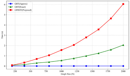
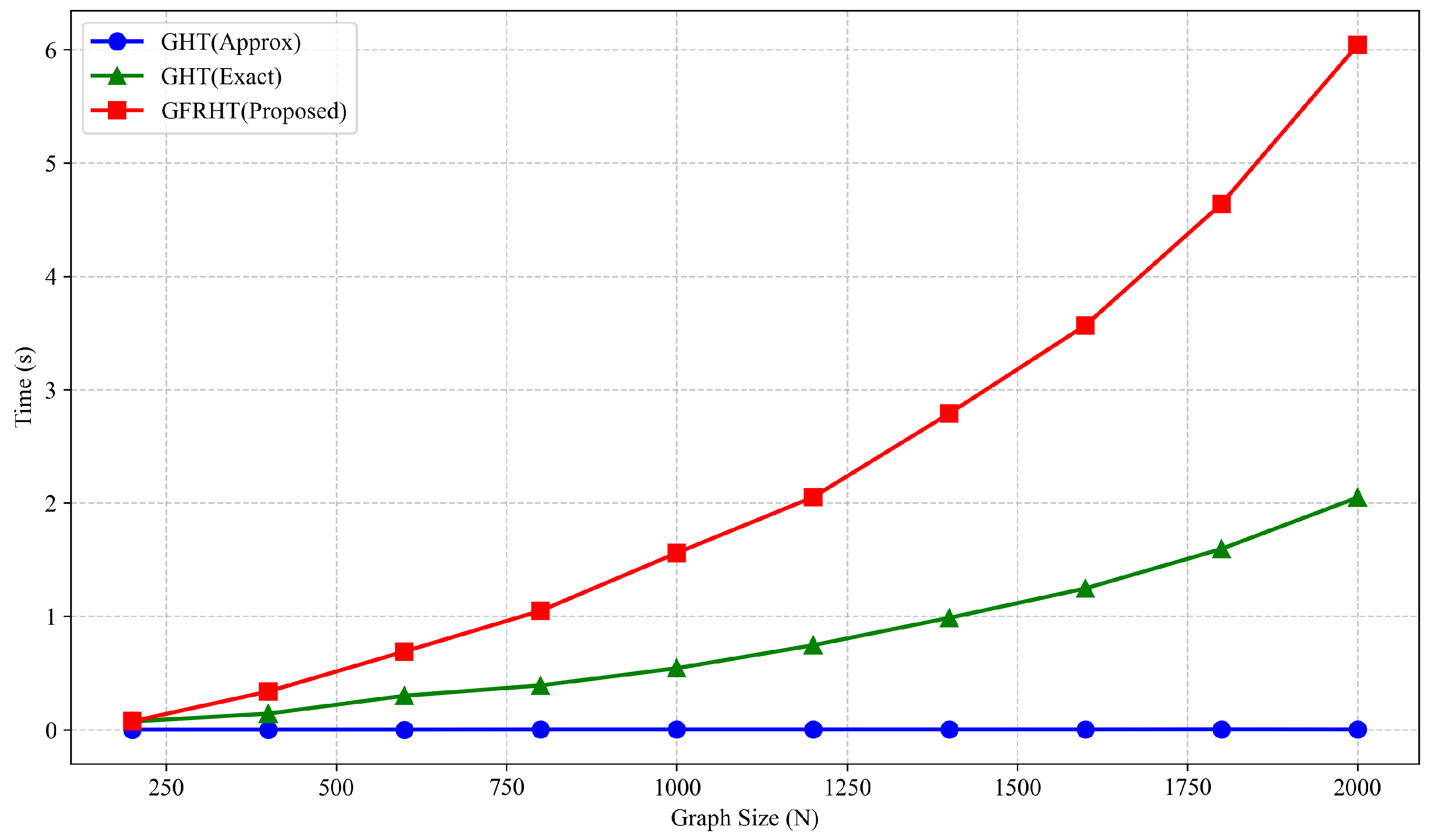
Consequently, the theoretical complexity involves four cubic-complexity operations ($\mathcal{O}\left(N^3\right)$). To empirically validate this, we conducted a runtime simulation on Erdős–Rényi random graphs ($p=0.05$) with sizes ranging from $N=200$ to $N=2000$. Figure 2 illustrates the execution time comparison. The results confirm that while the GHT approximation maintains a near-linear growth, the exact methods exhibit cubic growth. Notably, the GFRHT execution time is approximately 3 times that of the exact GHT. This increase, beyond the theoretical 2 times operational count, is attributed to the fact that the second eigen-decomposition in GFRHT is performed on the complex-valued GFT matrix $\mathbf{F}$, which is computationally more intensive than the initial decomposition of the real-valued adjacency matrix $\mathbf{A}$.

Figure 2. Empirical runtime comparison among three implementation strategies: (1) GHT Approx. (blue), using Chebyshev polynomial approximation ($K=20$); (2) GHT Exact (green), using a single eigen-decomposition; and (3) GFRHT (red), using dual eigen-decompositions. The results validate the theoretical complexity analysis: while the polynomial approximation scales linearly, the exact GHT exhibits cubic growth. The proposed GFRHT incurs an additional computational cost (approximately 3 times that of Exact GHT) due to the sequential dual eigen-decompositions and the complex arithmetic involved in processing the fractional operator.

Consequently, in the following application sections, we focus on scenarios where the graph size N is moderate, thereby mitigating the impact of the $\mathcal{O}\left(N^3\right)$ bottleneck.

3.3.4. Application to Graph Fractional Spectral Filtering

The GFRHT can be naturally viewed as a spectral filter in the fractional domain. Consider a noisy observation model $\mathbf{y}=\mathbf{Gx}+\mathbf{n}$, where $\mathbf{G}$ is a known transformation and $\mathbf{n}$ denotes additive noise. The operation ${\mathcal{H}}_{\alpha ,\beta }\left(\mathbf{y}\right)$ can be interpreted as a recovered signal obtained through a fractional spectral filter with coefficients ${\widehat{\mathbf{h}}}_{\beta }\left[k\right]$.

A significant advantage of the GFRHT over fixed filters is its adaptability. The parameters $(\alpha ,\beta )$ can be optimized for specific tasks, rather than being fixed a priori. In practice, they may be selected through grid search when the parameter space is small and discrete, or by applying gradient-based optimization strategies for efficient learning in continuous domains.

Formally, the optimal parameters are obtained by solving

$$({\alpha }^{*},{\beta }^{*})=arg\underset{\alpha ,\beta }{min}\mathbb{E}\left\{\parallel {\mathcal{H}}_{\alpha ,\beta }{\left(\mathbf{y}\right)-\mathbf{x}\parallel }_2^2\right\},$$

(22)

which minimizes the mean squared error (MSE) between the recovered signal and the ground truth.

While the optimization framework above presents a compelling application of the GFRHT, the core focus of this paper is to establish its foundational theory and explore its primary role in analytic signal generation and modulation analysis for feature extraction. Therefore, an empirical study of its performance in denoising, while a valuable direction for future research, falls beyond the scope of the present numerical validation. The simulations that follow in Section 3.4 are instead designed to systematically characterize the fundamental input-output behavior of the GFRHT transform itself for a clean signal $\mathbf{x}$.

3.4. Simulation Results of the GFRHT

In this section, we present a comprehensive numerical analysis using a directed social network as a case study to demonstrate the practical application and properties of the GFRHT. The network is represented by the adjacency matrix

$$\mathbf{A}=\left[\begin{array}{ccccc}0& 1& 1& 0& 1\\ 0& 0& 0& 1& 0\\ 0& 0& 0& 1& 0\\ 0& 0& 0& 0& 1\\ 1& 0& 0& 0& 0\end{array}\right],$$

where the five nodes correspond to individuals labeled as Alice (node 1), Bob (node 2), Charlie (node 3), David (node 4), and Eve (node 5). The directed edges represent influence relationships within this social network, with a value of 1 in position $(i,j)$ indicating that person i influences person j. This asymmetric connectivity pattern results in complex eigenvalues, which is essential for the GFRHT to produce meaningful transformations.

We define a graph signal $\mathbf{x}={[0.8,0.3,0.5,0.2,0.6]}^{\top }$ on these nodes, representing a measurable attribute such as activity level or opinion strength. To systematically investigate the behavior of the GFRHT, we select discrete values for the parameters $\alpha$ and $\beta$. Specifically, $\alpha$ is set to 0, ${\displaystyle \frac{1}{2}}$, and 1, while $\beta$ is set to 0, ${\displaystyle \frac{\pi }{4}}$, and ${\displaystyle \frac{\pi }{2}}$. The transform is then evaluated for all pairwise combinations of these values.

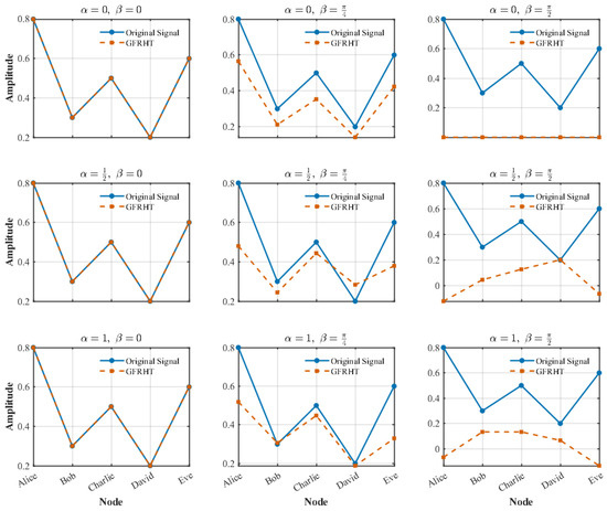
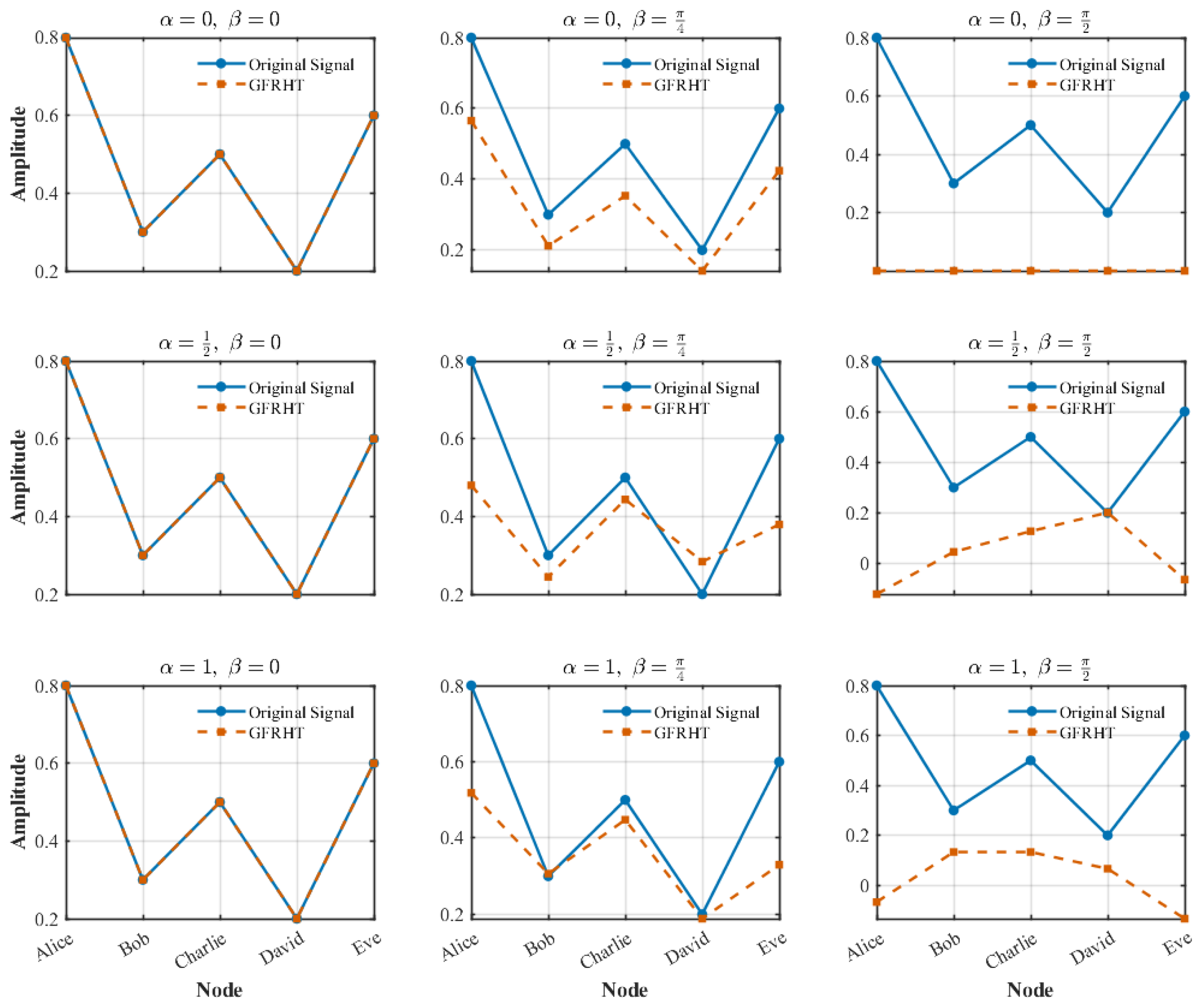
Figure 3 presents the transformation results for all parameter combinations. Each subplot shows the original signal (solid blue line) alongside the transformed signal (dashed vermilion line) for specific $\alpha$ and $\beta$ values. Several key observations emerge from this analysis:

Figure 3. Impact of fractional parameters on the GFRHT in a directed social network. This figure illustrates the transformation of a graph signal $\mathbf{x}$ (representing attribute intensity on 5 nodes: Alice to Eve) under varying fractional orders $\alpha$ and angle parameters $\beta$. The solid blue line represents the original input signal, and the dashed vermilion line represents the transformed GFRHT output. The rows correspond to fractional orders $\alpha =\{0,{\displaystyle \frac{1}{2}},1\}$, and the columns correspond to angles $\beta =\{0,{\displaystyle \frac{\pi }{4}},{\displaystyle \frac{\pi }{2}}\}$. As shown in the first column ($\beta =0$), the transform acts as an identity operator regardless of $\alpha$. The bottom-right subplot ($\alpha =1,\beta ={\displaystyle \frac{1}{2}}$) recovers the conventional GHT. Intermediate values (e.g., center plots) demonstrate how GFRHT modulates signal amplitude differently across nodes, offering flexible feature extraction capabilities beyond the fixed GHT.

First, when $\beta =0$ (i.e., the first column of subplots) for any $\alpha \in \{0,\frac{1}{2},1\}$, the GFRHT reduces to the identity operation, as expected from the definition of the GFRHT. This serves as a valuable validation of our implementation.

Second, as we increase $\beta$ while keeping $\alpha =0$, the GFRHT introduces progressively stronger modifications to the signal, demonstrating the role of $\beta$ in controlling the strength of the Hilbert transform component.

Third, the bottom-right subplot ($\alpha =1$, $\beta =\frac{\pi }{2}$) represents a special case where the GFRHT reduces to the conventional GHT. This case is particularly significant as it connects our generalized framework to the well-established GHT, providing a bridge between existing and proposed methodologies.

The systematic variation of both parameters reveals the flexibility of the GFRHT in modulating graph signals. Different parameter combinations emphasize different aspects of the structure of the signal, with some configurations amplifying certain features while suppressing others. This tunability makes the GFRHT a powerful tool for graph signal analysis, particularly in applications where certain frequency components or structural characteristics need to be emphasized or suppressed.

This numerical experiment demonstrates not only the computational feasibility of the GFRHT but also its practical utility in analyzing graph-structured data. The ability to tune both $\alpha$ and $\beta$ parameters provides researchers with a flexible framework for graph signal processing, enabling tailored analyses that can highlight different aspects of graph signals depending on the specific application requirements.

4. GFRAS

4.1. From GAS to GFRAS: A Generalized Analytic Signal

The conventional GAS, constructed via the GHT, is confined to the spectral domain and suffers from its inherent limitations. The flexibility of the GFRHT provides the necessary framework to generalize this concept. The GFRAS is defined to obtain a complex-valued representation of a real-valued graph signal whose properties—specifically its envelope (amplitude) and phase—can be examined in a proper fractional domain chosen by $\alpha$, and with a phase shift tailored by $\beta$.

4.2. Definition and Instantaneous Features

Building upon the proposed GFRHT, we define the GFRAS for a real-valued graph signal $\mathbf{x}$ as

$${\tilde{\mathbf{x}}}_{\alpha ,\beta }=\mathbf{x}+j{\mathcal{H}}_{\alpha ,\beta }\left(\mathbf{x}\right)={\mathbf{F}}^{-\alpha }(\mathbf{I}+j{\widehat{\mathbf{H}}}_{\beta }){\mathbf{F}}^{\alpha }\mathbf{x}.$$

(23)

Analogous to the conventional analytic signal, the GFRAS enables the derivation of several fundamental quantities for graph signal analysis, generalizing the concepts of amplitude, phase, and frequency modulation to the fractional-order graph setting. Specifically:

• Graph fractional amplitude modulation (GFRAM) is given by the magnitude of the GFRAS,

  $${\mathcal{A}}_{\alpha ,\beta }\left[k\right]=\left|{\tilde{\mathbf{x}}}_{\alpha ,\beta }\left[k\right]\right|=\sqrt{{\left(Re\left({\tilde{\mathbf{x}}}_{\alpha ,\beta }\left[k\right]\right)\right)}^2+{\left(Im\left({\tilde{\mathbf{x}}}_{\alpha ,\beta }\left[k\right]\right)\right)}^2}.$$

  (24)
• Graph fractional phase modulation (GFRPM) is defined as the phase angle of the GFRAS,

  $${\varphi }_{\alpha ,\beta }\left[k\right]=arctan\left({\displaystyle \frac{Im\left({\tilde{\mathbf{x}}}_{\alpha ,\beta }\left[k\right]\right)}{Re\left({\tilde{\mathbf{x}}}_{\alpha ,\beta }\left[k\right]\right)}}\right).$$

  (25)
• Graph fractional frequency modulation (GFRFM) is given by

  $${\omega }_{\alpha ,\beta }={\varphi }_{\alpha ,\beta }^u-\mathbf{A}{\varphi }_{\alpha ,\beta }^u,$$

  (26)

  where ${\varphi }_{\alpha ,\beta }^u$ denotes the unwrapped phase of the GFRAS. This generalizes the conventional GFM in Equation (9), reducing to it when $\alpha =1$ and $\beta =\frac{\pi }{2}$.

These modulation features provide a powerful tool for analyzing localized spectral behavior and modulations in graph signals within a vertex-frequency framework, effectively generalizing classical modulation concepts from time-frequency analysis to the fractional-order graph setting.

4.3. Physical Interpretation and Illustrative Analysis

To elucidate the physical significance of the fractional parameters $\alpha$ and $\beta$, we consider the problem of envelope extraction for non-stationary graph signals. The effectiveness of the Hilbert transform depends heavily on the domain in which the signal is analyzed.

The fractional order $\alpha$ governs the continuous interpolation between the vertex domain and the graph spectral domain. The conventional GHT operates strictly in the graph spectral domain ($\alpha =1$). However, for non-stationary signals (e.g., signals with varying frequency or localized transients), the signal energy is often spread out in the canonical spectral domain, leading to the Gibbs phenomenon and artifacts when the analytic signal is constructed. By tuning $\alpha$, the GFRHT searches for an optimal fractional domain where the signal’s energy distribution is most compact (sparse). In this optimal domain, the Hilbert operator can extract the instantaneous features with minimal leakage.

The angle parameter $\beta$ generalizes the phase shift. While the standard GHT imposes a rigid ${\displaystyle \frac{\pi }{2}}$ shift (orthogonalizing the signal), this assumption often violates the structure of graph signals with asymmetric spectra. Furthermore, the standard GHT nullifies components corresponding to real eigenvalues. The parameter $\beta$ allows for a flexible phase alignment and, crucially, preserves information at real eigenvalues through the $cos\beta$ term in the transfer function (Equation (15)), ensuring a complete signal representation.

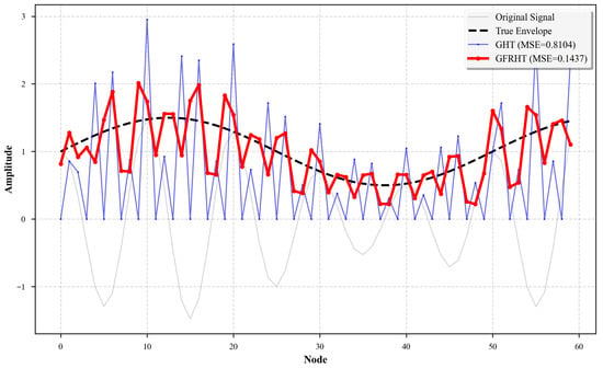
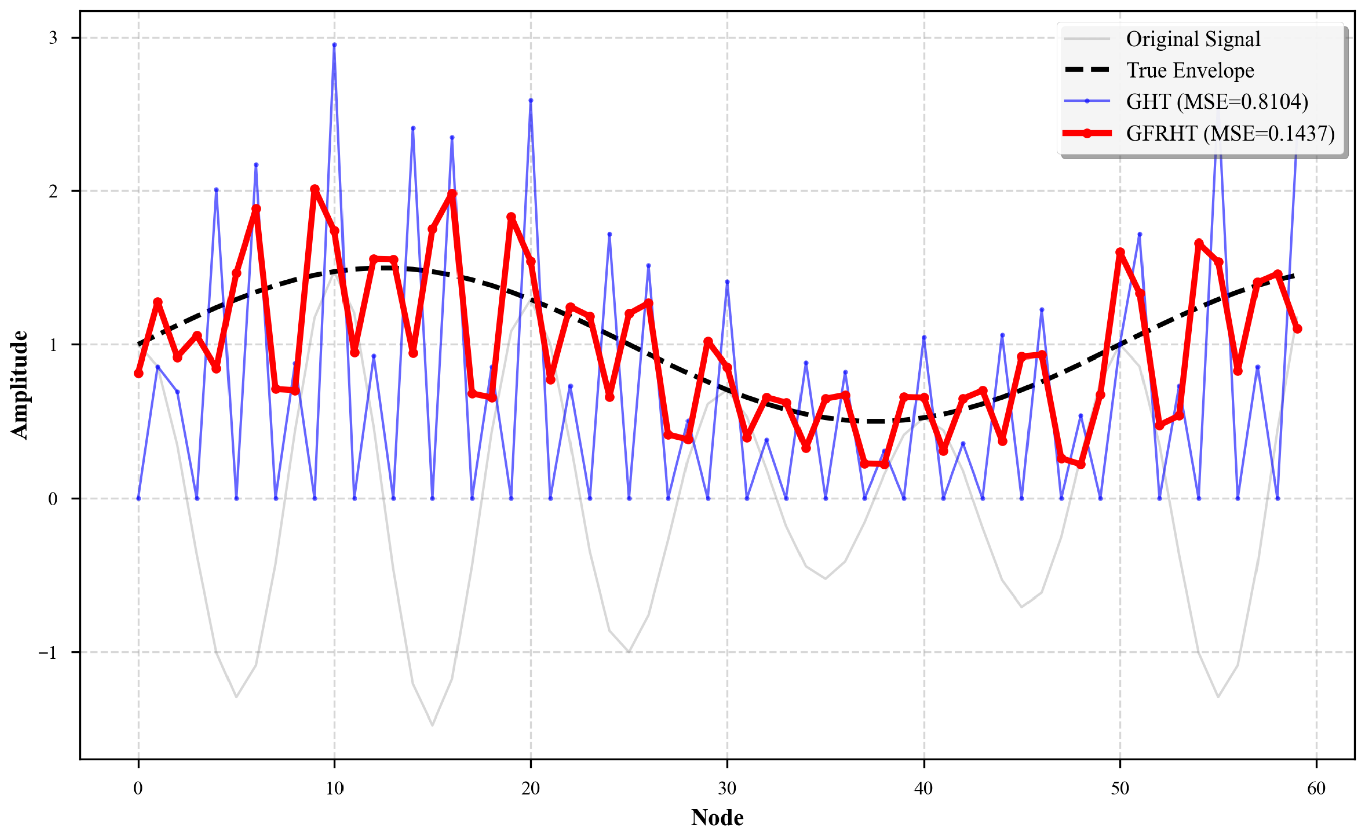
We visualize this effect in Figure 4, which compares the GFRAM extracted by GHT and GFRHT for a non-stationary signal on a directed cycle graph.

Figure 4. GFRAM on a directed cycle graph ($N=60$) for a non-stationary signal. The conventional GHT (blue line, $\alpha =1,\beta ={\displaystyle \frac{\pi }{2}}$) exhibits severe oscillations and fails to capture the low-frequency modulation trend due to its rigid spectral window (MSE = 0.8104). In contrast, the proposed GFRHT (red line), by tuning the fractional order and phase parameters ($\alpha ={\displaystyle \frac{1}{2}},\beta ={\displaystyle \frac{29\pi }{40}}$), changes the signal to the optimal domain where energy is concentrated. This results in a relatively smooth, physically meaningful envelope that closely matches the ground truth (black dashed line), achieving a significantly lower MSE of 0.1437.

• GHT Limitations: The conventional GHT (Figure 4, blue line) produces a highly volatile envelope with significant overshoot errors (MSE = 0.8104). This occurs because the fixed spectral basis vectors are ill-suited for representing the local variations of the non-stationary modulation.
• GFRHT Advantages: The proposed GFRHT (Figure 4, red line) adapts to the signal structure. With optimized parameters ($\alpha ={\displaystyle \frac{1}{2}},\beta ={\displaystyle \frac{29\pi }{40}}$), the transform aligns with the signal’s energy concentration, yielding a relatively smooth envelope that accurately tracks the ground truth (MSE = 0.1437). This confirms that $\alpha$ and $\beta$ serve as tunable lenses that focus the analysis on the physically relevant features of the graph signal.

4.4. Applications of the Extracted Features

The GFRAS provides a powerful multi-resolution tool for graph signal analysis. The key advantage over the conventional GAS is that by carefully selecting $\alpha$ and $\beta$, one can enhance certain signal features that might be obscured in the canonical domains. The extracted features enable numerous advanced applications:

1.

Anomaly detection: Anomalies often manifest as localized bursts of energy. The GFRAM ${\mathcal{A}}_{\alpha ,\beta }$ derived from a GFRAS, with parameters tuned to maximize the contrast between anomalous and normal regions, can yield a sharper and more localized energy map, significantly improving detection accuracy.

2.

Modulation analysis and demodulation: The GFRPM ${\varphi }_{\alpha ,\beta }$ can be used to track phase synchrony or the propagation of information waves on the graph. The parameter $\beta$ allows for adjusting the phase response to better align with the underlying modulation process, facilitating tasks like demodulation of graph-bandpass signals.

3.

Edge detection and feature extraction: In image processing applications represented on graphs (e.g., pixel grids), the fractional domain parameter $\alpha$ can be tuned to emphasize features at a particular scale. This can lead to more robust edge detection and texture classification across different image types, as the analysis is not locked into a single scale.

The adaptability of the GFRAS through its parameters makes it a versatile tool for a wide range of inference tasks on graphs, moving beyond the capabilities of fixed transforms.

5. Experiments

We next illustrate the applications of the proposed GFRHT on both synthesized and real-world signal examples, with a focus on its superior performance in tasks such as anomaly detection, speech signal classification and edge detection compared to the conventional GHT.

5.1. Anomaly Localization Under Varying Graph Densities

5.1.1. Experimental Setup

We construct a synthetic social network graph comprising 10 communities to validate the effectiveness of the proposed GFRHT in anomaly node localization tasks, with each community containing 6 nodes, resulting in a total of $N=60$ nodes. The network topology is designed as follows: intra-community edge weights are sampled from a uniform distribution $\mathcal{U}(0,1)$, reflecting strong connectivity within communities, while inter-community edge weights are drawn from $\mathcal{U}(0,0.5)$ and randomly placed between node pairs from different communities, forming a weighted and asymmetric adjacency matrix $\mathbf{A}$. Such graph structures with real edge weights are prevalent in practical applications such as road traffic analysis and brain connectivity studies.

Two distinct graph connectivity densities are considered to demonstrate the potential of our method:

• Sparse graph: Inter-community edges constitute 1% of the total possible edges in the graph.
• Dense graph: Inter-community edges constitute 10% of the total possible edges.

We normalize the adjacency matrix $\mathbf{A}$ such that its spectral radius $\rho \left(\mathbf{A}\right)=1$. Node labels correspond to the row indices of $\mathbf{A}$. We define a graph signal $\mathbf{x}$ to simulate localized anomalies, where $x_i=1$ for nodes $i=18$ to 23 (located in communities 3 and 4) and $x_i=0$ elsewhere. We then process this signal using both the conventional GHT and the proposed GFRHT (with initial parameters $(\alpha ,\beta )=({\displaystyle \frac{11}{10}},{\displaystyle \frac{\pi }{20}})$) to highlight anomalous nodes in the transform domain.

To determine the optimal parameters, we perform a fine-grained grid search centered around initial parameters $(\alpha ,\beta )=({\displaystyle \frac{11}{10}},{\displaystyle \frac{\pi }{20}})$. The search range is set to $\alpha \in [0.95,1.25]$ and $p\in [0.05,0.35]$ (where $\beta =p·{\displaystyle \frac{\pi }{2}}$). This analysis identified the optimal configuration as $(\alpha =1,\beta ={\displaystyle \frac{\pi }{20}})$, which is subsequently used for the GFRHT results reported below.

5.1.2. Results and Analysis

For objective performance evaluation, three quantitative metrics are employed: signal-to-noise ratio (SNR, dB), localization precision (Precision@k), and root mean square error (RMSE).

The SNR is defined as

$${\mathrm{SNR}}_{\mathrm{dB}}=20{log}_{10}\left({\displaystyle \frac{{\mu }_{\mathrm{anomaly}}}{{\sigma }_{\mathrm{background}}}}\right),$$

(27)

where ${\mu }_{\mathrm{anomaly}}$ denotes the mean response magnitude at the ground-truth anomaly nodes, and ${\sigma }_{\mathrm{background}}$ is the standard deviation of the responses at all non-anomaly nodes.

The localization precision at top-k nodes (Precision@k) is computed as

$$\mathrm{Precision}@k={\displaystyle \frac{|\mathcal{T}\cap {\mathcal{P}}_k|}{k}},$$

(28)

where $\mathcal{T}$ is the set of true anomaly indices and ${\mathcal{P}}_k$ is the set of top-k nodes ranked by the response magnitude.

The RMSE between the estimated response $\mathbf{y}$ and the ground-truth anomaly indicator $\mathbf{g}$ is given by

$$\mathrm{RMSE}=\sqrt{{\displaystyle \frac{1}{N}}\sum _{i=1}^N{(y_i-g_i)}^2}.$$

(29)

Table 3 summarizes the comparative performance of GHT and GFRHT under both sparse and dense graph configurations.

Table 3. Comparative performance of GHT and GFRHT for anomaly localization under sparse and dense graph structures.

Graph Type	Method	SNR (dB)	Precision@6	RMSE
Sparse Graph	GHT	$11.16$	$0.667$	$0.2131$
	GFRHT	$\mathbf{39.69}$	$\mathbf{1.000}$	$\mathbf{0.0202}$
Dense Graph	GHT	$-2.41$	$0.000$	$0.3883$
	GFRHT	$\mathbf{18.80}$	$\mathbf{1.000}$	$\mathbf{0.1460}$

Note: Bold values indicate the optimal performance for each metric.

The optimized GFRHT demonstrates exceptional performance. In the sparse graph, it achieves an SNR of 39.69 dB, representing a 28.53 dB improvement over the conventional GHT. Notably, the RMSE is reduced to 0.0202. In the dense graph, where GHT fails (SNR = −2.41 dB), GFRHT recovers the signal with an SNR of 18.80 dB and achieves perfect localization precision (Precision@6 = 1.000). These results, updated based on the sensitivity analysis, which will be shown in Section 5.6, underscore the critical importance of the tunable phase parameter $\beta$ even when operating near the standard spectral domain ($\alpha \approx 1$).

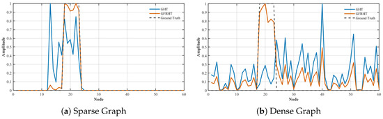
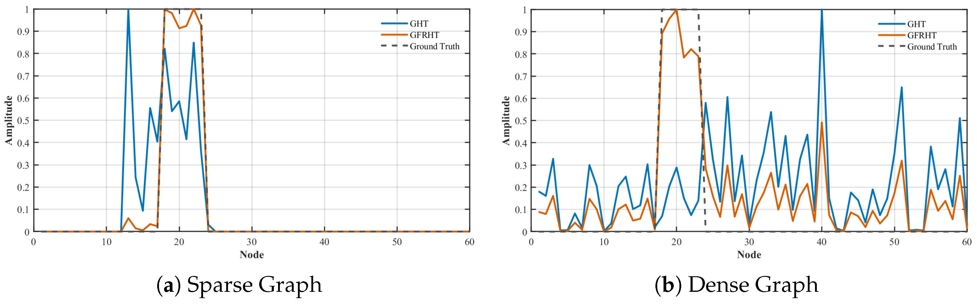
Figure 5 provides a visual illustration of these findings. For the sparse graph, the output of GFRHT exhibits sharper peaks concentrated around the anomalous region (Nodes 18–23), with minimal background response. For the dense graph, the output of GHT is contaminated by numerous artifacts, making anomaly identification impossible; whereas GFRHT successfully suppresses background noise, clearly highlighting the locations of the anomalous nodes.

Figure 5. Visual comparison of anomaly localization performance. (a,b) display the output magnitudes of the GHT and the proposed GFRHT for the sparse and dense graph configurations, respectively. The proposed GFRHT produces sharp, concentrated peaks precisely at the true anomaly nodes (18–23) with minimal background artifacts, demonstrating superior precision and noise robustness under both connectivity regimes.

In summary, both quantitative and qualitative results confirm that GFRHT not only consistently outperforms GHT across all scenarios but, more importantly, maintains excellent localization performance even in dense graph environments where GHT completely fails. This robust performance firmly establishes the effectiveness of the fractional operator in enhancing the localization properties and resilience of the transform, offering a reliable solution for precise anomaly detection in complex networks.

5.1.3. Discussion

The experimental results presented in Section 5.1.2 unequivocally demonstrate the superior performance of the proposed GFRHT over the conventional GHT for the task of anomaly localization in graph signals. This discussion aims to elucidate the underlying reasons for this performance gap and explore the broader implications of our findings.

The fundamental advantage of GFRHT stems from the additional degrees of freedom provided by the fractional order $\alpha$ and angle $\beta$. While the classical GHT applies a fixed, binary spectral filter ($\pm j$), the fractional framework allows for a more nuanced and continuous modulation of the frequency components of the graph. This flexibility is crucial for adapting to the specific topology of the graph. In the dense graph scenario, where excessive inter-community connections cause signal energy to diffuse uncontrollably, the rigid filter of the GHT is unable to isolate the anomaly. The GFRHT, parameterized here with $\alpha =1,\beta ={\displaystyle \frac{\pi }{20}}$, effectively acts as a customized filter that suppresses this spurious diffusion, thereby concentrating the energy of the transform around the true anomalous nodes. This explains the dramatic recovery in SNR from −2.41 dB (GHT) to 18.80 dB (GFRHT) and the leap in precision from 0% to 100%.

Furthermore, the perfect Precision@6 score achieved by GFRHT in both sparse and dense configurations is a particularly significant result. It indicates that the method not only enhances the contrast between signal and noise but also perfectly preserves the rank ordering of the anomalous nodes within the output. This property is paramount for practical applications where identifying the exact set of most likely anomalous nodes is required, rather than just a diffuse anomalous region.

The observed performance also highlights the robustness of the GFRHT framework. Its exceptional performance across two vastly different graph densities—from a near-block-diagonal structure to a highly connected one—suggests that the method is not overly sensitive to specific topological configurations. This robustness is a desirable property for analyzing real-world networks, which often exhibit complex and varied connection patterns.

5.2. Detection of Diverse Anomaly Types Across Graph Topologies

5.2.1. Experimental Setup

We generate two types of graphs with distinct topological properties: community graphs and scale-free graphs, each containing $N=50$ nodes. The adjacency matrix $\mathbf{A}$ of each graph is normalized to ensure its spectral radius $\rho \left(\mathbf{A}\right)=1$, which is a standard preprocessing step in graph signal processing.

For each graph type, we introduce three fundamentally different types of anomalies with specific characteristics:

• Low-frequency anomaly: The graph signal is constructed by emphasizing the smoothest eigenvector ${\mathbf{v}}_{min}$ of $\mathbf{A}$ (associated with the smallest eigenvalue magnitude $\left|\lambda \right|$), scaled by a factor of 3. Localized perturbations are then introduced by increasing the amplitude by 1.5 at exactly $k=3$ randomly selected nodes.
• High-frequency anomaly: The signal is formed by a linear combination of the two most oscillatory eigenvectors (${\mathbf{v}}_{{max}_1}$ and ${\mathbf{v}}_{{max}_2}$): $\mathbf{x}={\mathbf{v}}_{{max}_1}+0.3{\mathbf{v}}_{{max}_2}$. The amplitude is increased by 1.5 at $k=5$ randomly chosen nodes.
• Impulse anomaly: The signal $\mathbf{x}$ is set to zero at all nodes except for exactly $k=4$ randomly selected nodes, where its value is set to 2.

All generated signals are further corrupted by additive white Gaussian noise with a standard deviation of 0.1. Both the conventional GHT with fixed parameters ($\alpha =1,\beta =\frac{\pi }{2}$) and the proposed GFRHT are applied to each graph-anomaly combination. For GFRHT, an exhaustive grid search is conducted over the parameter space, with $\alpha \in [0,2]$ sampled at intervals of $0.1$, and $\beta =p·{\displaystyle \frac{\pi }{2}}$ where $p\in [0,2]$ is sampled at intervals of $0.1$. The objective is to determine the optimal parameter configuration by solving

$$({\alpha }^{*},{\beta }^{*})=arg\underset{\alpha ,\beta }{max}\mathrm{SNR}(\alpha ,\beta ),$$

(30)

where SNR is the detection metric defined in Equation (27).

5.2.2. Results and Analysis

The experimental results unequivocally demonstrate the exceptional performance enhancement achieved by the proposed GFRHT framework compared to the conventional GHT. As quantitatively summarized in Table 4, the GFRHT yields extraordinary performance improvements ranging from 361.0% to an unprecedented 4137.4% across diverse experimental conditions.

Table 4. Performance comparison between the conventional GHT and the proposed GFRHT for anomaly detection. The optimal parameters (${\alpha }^{*},{\beta }^{*}$) for GFRHT are determined via grid search.

Graph Type	Anomaly Type	${\mathit{\alpha }}^{*}$	${\mathit{\beta }}^{*}$	GHT SNR (dB)	GFRHT SNR (dB)	Improvement 1
Community	Low-Frequency	$\frac{7}{5}$	$\frac{9\pi }{10}$	$1.97$	$\mathbf{9.08}$	$+361.0$%
	High-Frequency	$\frac{7}{5}$	$\pi$	$1.36$	$\mathbf{13.59}$	$+900.1$%
	Impulse	$\frac{1}{10}$	$\frac{19\pi }{20}$	$0.69$	$\mathbf{29.12}$	$+4137.4$%
Scale-Free	Low-Frequency	$\frac{11}{10}$	$\frac{9\pi }{20}$	$0.64$	$\mathbf{5.22}$	$+719.8$%
	High-Frequency	$\frac{1}{5}$	$\frac{\pi }{10}$	$0.39$	$\mathbf{12.55}$	$+3150.6$%
	Impulse	$\frac{7}{5}$	$\frac{\pi }{20}$	$1.31$	$\mathbf{24.84}$	$+1791.8$%

Note: ¹ Calculated from the dB gain relative to the GHT baseline; bold values indicate the optimal performance. Context: The proposed GFRHT consistently achieves higher SNR values, indicating superior separation between anomalous nodes and background noise compared to the fixed-parameter GHT.

The optimal fractional parameters exhibit mathematically significant patterns that reflect the intrinsic characteristics of each anomaly type. For low-frequency anomalies, the optimal parameters converge around ${\alpha }^{*}=\frac{7}{5}$ and ${\beta }^{*}=\frac{9\pi }{10}$ for community graphs, while scale-free graphs prefer ${\alpha }^{*}=\frac{11}{10}$ and ${\beta }^{*}=\frac{9\pi }{20}$. This configuration indicates that moderately smooth fractional transforms combined with specific phase modifications significantly enhance detection of slow-varying anomalies.

For high-frequency anomalies, the optimal parameters demonstrate substantial diversity, with ${\alpha }^{*}$ values ranging from $\frac{7}{5}$ to $\frac{1}{5}$ and ${\beta }^{*}$ values spanning from $\pi$ to $\frac{\pi }{10}$. This variability underscores the necessity of precise parameter tuning to match the unique spectral characteristics of different graph topologies when detecting oscillatory patterns.

Most remarkably, the GFRHT framework exhibits extraordinary efficacy for impulse anomaly detection, achieving unprecedented improvements of 4137.4% and 1791.8% for community and scale-free graphs, respectively. The optimal parameters for impulse anomalies reveal extreme values, with ${\alpha }^{*}$ as low as $\frac{1}{10}$ and ${\beta }^{*}$ approaching $\pi$ ($\frac{19\pi }{20}$), indicating that specific fractional orders profoundly enhance the detection of sparse, impulsive disturbances.

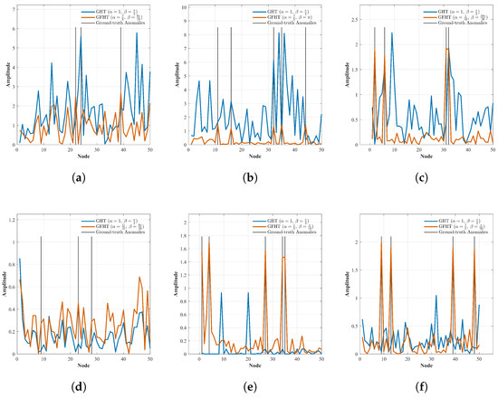
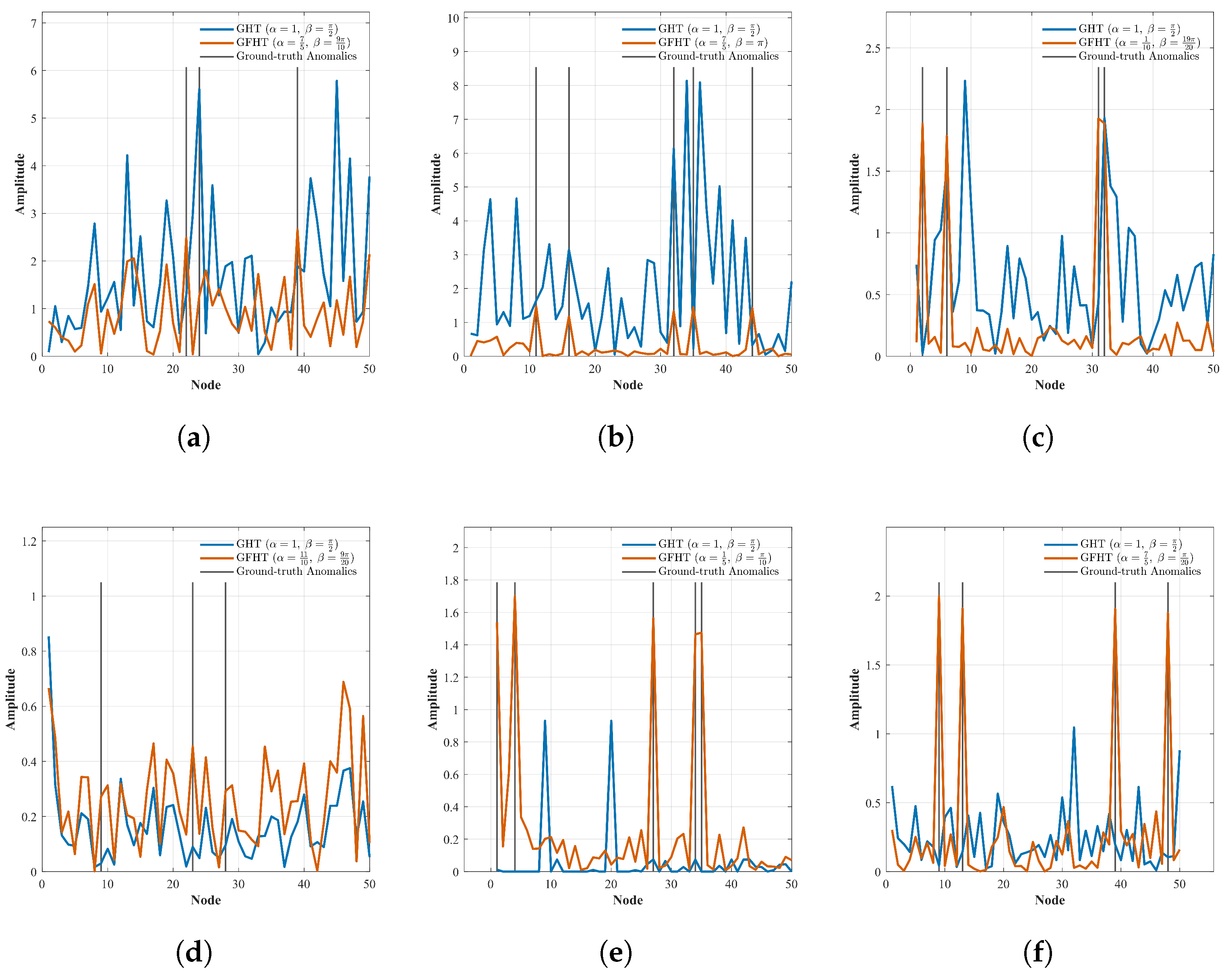
Figure 6 provides comprehensive visual evidence supporting the quantitative findings presented in Table 4. The visualization clearly illustrates the superior detection performance of GFRHT across all graph topologies and anomaly types. In each subfigure, the GFRHT response (shown in vermilion) demonstrates significantly sharper and more distinct peaks at the ground-truth anomaly locations compared to the GHT response (shown in blue).

Figure 6. Comparative visualization of anomaly localization performance across varying graph topologies and anomaly types. The plots compare the signal magnitude of the proposed GFRHT against the baseline GHT and the ground truth. The top row (a–c) displays results on Community Graphs, while the bottom row (d–f) displays results on Scale-Free Graphs. The columns represent three distinct anomaly types: Low-Frequency (a,d), High-Frequency (b,e), and Impulse (c,f). Blue solid line: Conventional GHT output. Vermilion solid line: Proposed GFRHT output (using optimal $\alpha ,\beta$). Gray vertical solid lines: Ground truth locations of the anomalies. In all scenarios, the GFRHT produces sharp, distinct peaks that align precisely with the ground truth anomalies (gray solid lines), significantly suppressing background noise. In contrast, the conventional GHT (blue) often exhibits spurious peaks and higher noise floors, particularly in high-frequency and impulse anomaly cases (e.g., subplots (c,f)).

For community graphs with low-frequency anomalies (Figure 6a), the GFRHT response exhibits enhanced sensitivity to the smooth variations characteristic of this anomaly type. Similarly, for high-frequency anomalies on community graphs (Figure 6b), the GFRHT effectively captures the oscillatory patterns while suppressing background noise. Most impressively, for impulse anomalies on community graphs (Figure 6c), the GFRHT produces exceptionally sharp and localized responses precisely at the anomaly locations.

The same trend is observed for scale-free graphs, where the GFRHT consistently outperforms the baseline GHT across all anomaly types (Figure 6d–f). The visual results confirm the remarkable quantitative improvements reported in Table 4, particularly the order-of-magnitude enhancements for impulse and high-frequency anomalies.

5.2.3. Discussion

The results demonstrate that the GFRHT is highly effective in detecting anomalies, especially for low-frequency, high-frequency, and impulse anomalies. The substantial improvements in SNR indicate that the GFRHT is better at distinguishing anomalies from normal behavior, which is crucial for applications in network anomaly detection, signal processing, and other areas where detecting unusual patterns is critical.

5.3. Anomaly Detection in Real-World Sensor Networks via Learnable GFRHT

To rigorously evaluate the generalizability of GFRHT on irregular graph topologies, we conducted an experiment using the Molene Weather Dataset [44,45]. The dataset contains hourly temperature recordings from 32 weather stations in Brittany, France.

5.3.1. Graph Construction and Setup

Unlike the synthetic graphs used in previous sections, the topology of this sensor network is determined by physical geography. We constructed a K-nearest neighbor graph ($K=5$) based on the Euclidean distance between the stations’ geographical coordinates (latitude and longitude). The graph signal $\mathbf{x}$ represents the normalized temperature readings. To simulate a challenging multi-failure scenario, we injected impulse anomalies into $N_{anom}=10$ randomly selected stations on top of the real temperature background, followed by additive Gaussian noise ($\sigma =0.2$).

5.3.2. Learnable Parameter Optimization

Instead of a discrete grid search, we formulated the parameter selection as a differentiable optimization problem. We treat $\alpha$ and $\beta$ as learnable parameters and optimize them using the Adam algorithm to minimize the RMSE of the anomaly detection envelope. This demonstrates the potential of GFRHT to be integrated as a trainable layer in end-to-end graph neural networks.

5.3.3. Results and Analysis

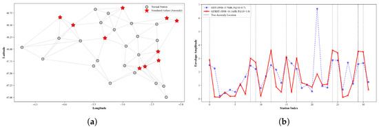
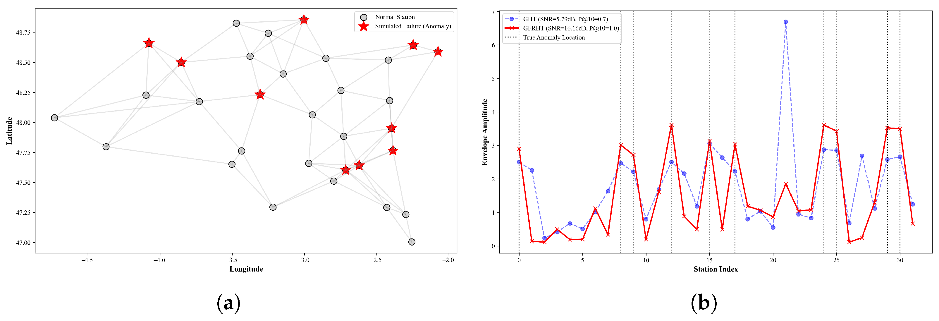
Table 5 and Figure 7 summarize the performance comparison. The optimization converged to $\alpha =0.27$ and $\beta =0.12$. This low fractional order suggests that for this specific irregular topology, the optimal domain for separating anomalies from the smooth temperature background lies closer to the vertex domain than the spectral domain. The conventional GHT ($\alpha =1,\beta ={\displaystyle \frac{\pi }{2}}$) struggled with the irregular topology, achieving a Precision@10 of only 0.70 and an SNR of 5.79 dB. In contrast, the proposed Learnable GFRHT perfectly identified all 10 anomalies (Precision@10 = 1.00) and achieved an SNR of 16.16 dB, representing a 10.37 dB improvement.

Table 5. Performance Comparison of Different Methods.

Metric	GHT	GFRHT ($\mathit{\alpha }=0.27,\mathit{\beta }=0.12$)	Improvement
SNR (dB)	5.79	$\mathbf{16.16}$	+10.37 dB
Precision@10	0.700	$\mathbf{1.000}$	+42.9%
RMSE	0.4241	$\mathbf{0.2011}$	−52.6%

Note: Bold values indicate the optimal performance for each metric.

Figure 7. Anomaly detection on the Molene real-world sensor network.(a) Real Sensor Topology and Injected Anomalies (10 Failure Nodes). The graph topology constructed from actual geographical coordinates, with 10 simulated sensor failures (red stars). (b) Anomaly Detection Envelope GFRHT($\alpha =0.27,\beta =0.12$). The comparison of detection envelopes. The conventional GHT (blue dashed line) fails to distinguish some anomalies from background noise due to the irregular graph structure. The proposed learnable GFRHT (red solid line), with automatically optimized parameters ($\alpha =0.27,\beta =0.12$), produces sharp peaks precisely at the true anomaly locations, achieving perfect detection (Precision@10 = 1.0).

5.3.4. Discussion

The results above confirm that the dual-parameter flexibility of GFRHT is essential for handling the complex spectral characteristics of real-world irregular networks. Specifically, the learned fractional order ($\alpha =0.27$) indicates that real-world temperature signals exhibit strong spatial smoothness, requiring an analysis domain that deviates significantly from the standard spectral domain ($\alpha =1$). By adaptively finding this optimal domain, GFRHT overcomes the limitations of the fixed GHT.

5.4. Speech Classification Using the GFRAM and GFRFM

We extend the application of the proposed GFRHT to a comprehensive speech classification benchmark, aiming to thoroughly validate its effectiveness and generalizability. The primary objective is to investigate whether the GFRAM and GFRFM features, derived from the GFRHT, provide complementary information that enhances classification performance beyond conventional and standard graph-based features.

5.4.1. Experimental Setup

A comprehensive binary classification benchmark is established to evaluate the proposed features. The benchmark encompasses four distinct tasks to test generalizability: Gender Classification (male vs. female), Emotion Classification (happy vs. angry), Language Classification (Chinese vs. English), and Age Group Classification (minor vs. adult). Speech data are segmented into frames of length $N=50$.

A graph representation of the speech signal is learned from a separate dataset to capture the intrinsic structure of the speech frames. The adjacency matrix ${\mathbf{A}}^{*}$ is obtained by solving the following optimization problem, and stability is ensured through appropriate constraints:

$${\mathbf{A}}^{*}=arg\underset{\mathbf{A}}{min}{\parallel {\mathbf{X}}_l-\mathbf{A}{\mathbf{X}}_l\parallel }_2^2\mathrm{subject}\mathrm{to}diag\left(\mathbf{A}\right)=\mathbf{0},\mathbf{A}\mathbf{1}=\mathbf{1},{\mathbf{A}}^{\mathsf{T}}\mathbf{1}=\mathbf{1}$$

(31)

where ${\mathbf{X}}_l$ is the training data matrix. This learned graph serves as the foundation for all subsequent graph-based feature extraction.

Six different classifiers were compared, each leveraging a unique combination of feature extraction methods:

• DFT-based: Uses the magnitudes of the discrete Fourier transform (DFT) coefficients of the conventional 1D AM and FM.
• GFT-based: Uses the magnitudes of the GFT coefficients of the GAM and GFM.
• DFT + GFT: A concatenation of the feature vectors from the DFT-based and GFT-based classifiers.
• DFRFT-based: Uses the magnitudes of the discrete FRFT (DFRFT) coefficients of the 1D AM and FM. The order parameters are treated as learnable parameters and are optimized jointly with the classifier weights via gradient descent.
• GFRFT-based: Uses the magnitudes of the GFRFT coefficients of the GFRAM and GFRFM. The fractional order $\alpha$ and angle $\beta$ parameters are treated as learnable parameters and are optimized jointly with the classifier weights via gradient descent.
• DFRFT + GFRFT: A concatenation of the feature vectors from the DFRFT-based and GFRFT-based classifiers. This represents our most comprehensive feature set, combining the strengths of fractional transforms in both classical and graph domains.

A two-layer neural network is employed as the classifier. The number of neurons in the hidden layer is treated as a tunable hyper-parameter to find a balance between model capacity and computational complexity. The models are trained and tested on data that is strictly held out from the set ${\mathbf{X}}_l$ used for graph learning. Performance metrics are averaged over multiple runs with random data partitions to ensure statistical significance.

5.4.2. Results and Analysis

A.

Performance Across Diverse Classification Tasks

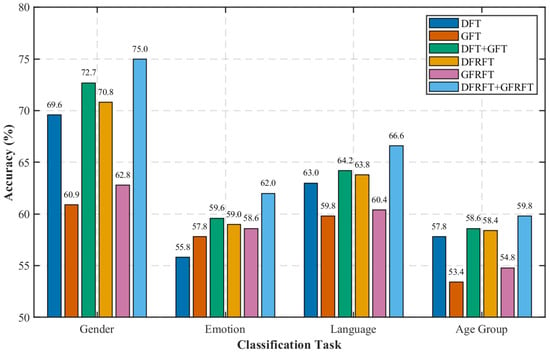
The comprehensive classification accuracies across all four tasks and feature sets are summarized in Figure 8. The results lead to several critical observations:

Figure 8. Classification accuracy comparison across different tasks. The proposed DFRFT + GFRFT fusion method consistently achieves the highest performance.

1.

Superiority of fractional graph features: The proposed DFRFT + GFRFT fusion method consistently achieves the highest accuracy across all four classification tasks, demonstrating the universal effectiveness of the fractional features.

2.

Significant performance gain: The DFRFT + GFRFT combination provides a substantial improvement over the previously best-performing DFT + GFT combination, with relative performance gains of 3.16%, 4.03%, 3.74%, and 2.05% for gender, emotion, language, and age classification tasks, respectively. This confirms our hypothesis that the fractional transforms capture unique, complementary information.

3.

The power of fusion: The performance hierarchy (DFRFT + GFRFT > DFT + GFT > single-method features) underscores the consistent benefit of feature fusion. Integrating information from both the classical and graph domains, and further enhancing it with fractional orders, yields a more robust and discriminative feature representation.

B.

Scalability and Data Efficiency with Increasing Sample Size

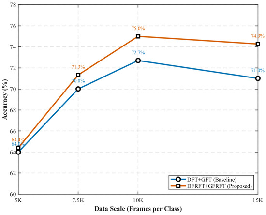
To investigate the scalability of the proposed method, we evaluate its performance on the gender classification task with increasing amounts of training data. The results, detailed in Table 6 and Figure 9, reveal a crucial trend: the performance advantage of the proposed DFRFT+GFRFT fusion method is maintained across data scales.

Table 6. Classification accuracy (%) for the gender task under different data scales.

Data Scale (Frames)	DFT	GFT	DFT + GFT	DFRFT	GFRFT	DFRFT + GFRFT
5000	62.20	53.20	64.00	63.00	58.40	64.40
7500	65.47	59.07	70.00	67.07	59.87	71.33
10,000	69.60	60.90	72.70	70.80	62.80	75.00
15,000	68.80	61.87	71.00	70.53	62.20	74.27

Note: Bold values indicate the optimal performance.

Figure 9. Accuracy variation curves of different feature combinations with data scale for the gender classification task.

This analysis yields two key insights: (i) Consistent superiority: The DFRFT + GFRFT fusion strategy consistently outperforms all other methods at every data scale, demonstrating its robustness and reliability; (ii) Performance trend: The accuracy of both the baseline and proposed methods shows a strong positive correlation with the amount of data from 5000 to 10,000 frames, achieving peak performance at the 10,000-frame scale. The observed slight performance degradation at the 15,000-frame mark for both methods is analyzed in Section 5.4.3.

5.4.3. Discussion

The experimental results from both diverse tasks and varying data scales unequivocally demonstrate that the features derived from the proposed GFRHT framework provide a significant and robust advantage for speech classification.

The superior performance of the DFRFT + GFRFT classifier establishes that:

• Fractional transforms offer a richer representation: By enabling analysis in an optimal fractional domain, the DFRFT and GFRFT uncover subtle, discriminative features in the speech signal that are lost in the conventional Fourier or graph Fourier domains.
• Synergy between domains: The classical (DFRFT) and graph-based (GFRFT) fractional transforms are not redundant; they capture complementary aspects of the structure of the signal. Their fusion creates a more powerful feature set than any single method can provide.
• Data-effective and robust: The method not only works well on limited data but also maintains its advantage across different data scales, making it suitable for real-world applications.

Analysis of Performance at Largest Data Scale: The observed performance plateau and slight decrease at the largest data scale (15,000 frames) for both methods is attributed to the fixed capacity of the neural network classifier, which is kept constant across all data scales. While sufficient for smaller datasets, this fixed capacity becomes a limiting bottleneck for larger datasets, preventing further learning. Crucially, the performance gap between the proposed and baseline methods persists even at this scale. This indicates that the quality of the features extracted by DFRFT + GFRFT remains superior, and the performance ceiling is imposed by the classifier itself, not the feature extraction front-end.

5.5. Edge Detection Using the GFRHT

5.5.1. Experimental Setup

Last, we investigate the performance of the GFRHT for edge detection in 2D images. The GFRHT, which generalizes the conventional GHT by incorporating two parameters, offers enhanced flexibility in edge detection. To evaluate its effectiveness, we apply the GFRHT to two 40 × 40 test images: a synthetic image and a gear image.

The graph structure for the image is defined by connecting the j-th pixel in the i-th row to the $(j+1)$-th pixel in the same row and the j-th pixel in the $(i+1)$-th row. The adjacency matrix of this graph is consequently given by the Kronecker product $\mathbf{A}=\mathbf{C}\otimes \mathbf{C}$, where

$$\mathbf{C}=\left(\begin{array}{ccccc}0& 1& 0& \dots & 0\\ 0& 0& 1& \dots & 0\\ ⋮& ⋮& ⋮& \ddots & ⋮\\ 1& 0& 0& \dots & 0\end{array}\right).$$

(32)

This graph serves as the shift operator for the subsequent application of the proposed GFRHT. All performance comparisons between the GFRHT and the conventional GHT are conducted under this identical graph construction.

5.5.2. Results and Analysis

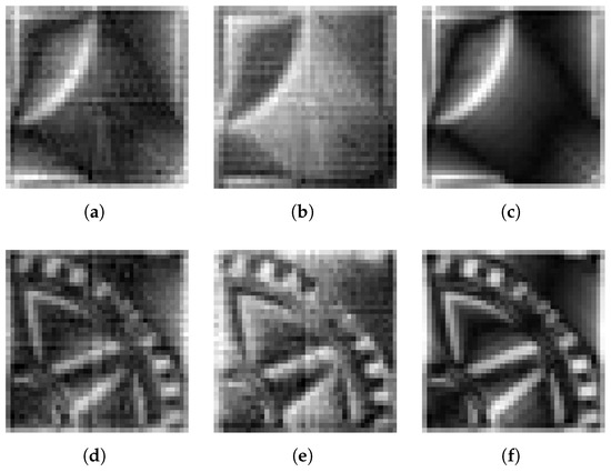
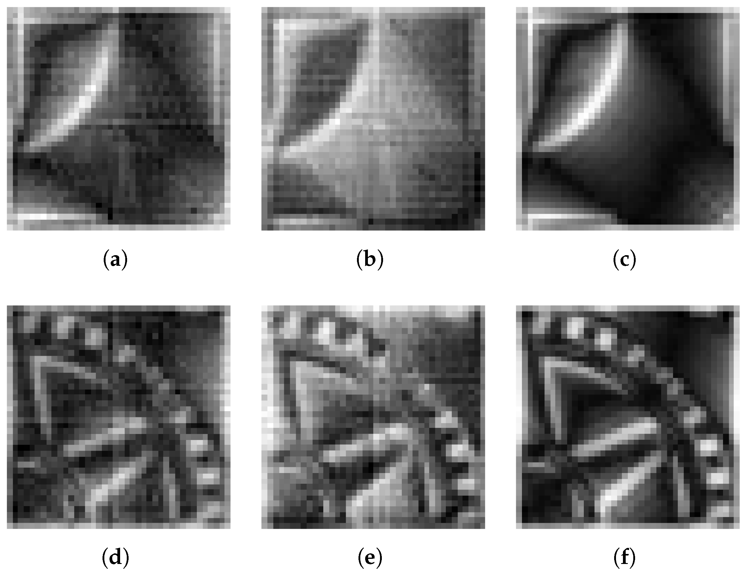
Figure 10 shows the original images and their respective results after applying the GHT and GFRHT. In both cases, the GFRHT produces sharper, more distinct edges compared to the GHT, particularly in complex regions of the images. This is evidenced by the clearer delineation of boundaries in the gear image, which contains intricate edge structures.

Figure 10. Edge detection comparison. (a) Synthetic and (d) gear original images; (b,e) are results from the GHT; (c,f) are results from the proposed GFRHT. The GFRHT provides sharper edges and superior contour continuity, as demonstrated with parameters $(\alpha ,\beta )=(\frac{7}{10},{\displaystyle \frac{\pi }{10}})$ for the synthetic image and $(\alpha ,\beta )=(\frac{4}{5},\frac{3\pi }{20})$ for the gear image.

Quantitative results further confirm the superior performance of the GFRHT. As shown in Table 7, we evaluate edge detection performance using standard metrics: information entropy, structural similarity index (SSIM), and edge density. The GFRHT consistently outperforms the GHT in all metrics, with higher information entropy, SSIM values, and edge density, indicating that the GFRHT provides better edge clarity and preserves more detail in the images.

Table 7. Quantitative comparison between GHT and the proposed GFRHT.

Graph Type	Metric	GHT	GFRHT	Improvement
Synthetic Image	Information Entropy	0.8424	0.9037	+7.3%
	SSIM	0.1305	0.7949	+509%
	Edge Density	0.2706	0.3194	+18.0%
Gear Image	Information Entropy	0.7909	0.8910	+12.7%
	SSIM	0.0784	0.8372	+968%
	Edge Density	0.2375	0.3081	+29.7%

Note: Bold values indicate the optimal performance for each metric.

5.5.3. Discussion

The experimental results demonstrate that GFRHT is highly effective for edge detection, especially in images exhibiting complex edge structures. The ability of GFRHT to accentuate fine details while preserving sharp boundaries represents a clear advantage over the conventional GHT. This enhanced performance arises from the flexibility afforded by the two tunable parameters $\alpha$ and $\beta$, which enable more precise control of the transformation. The higher values observed in the information entropy, SSIM, and edge density metrics suggest that the GFRHT not only enhances edge detection but also improves the overall image representation, making it a promising tool for applications requiring accurate edge detection and feature extraction.

5.6. Unified Parameter Sensitivity Analysis

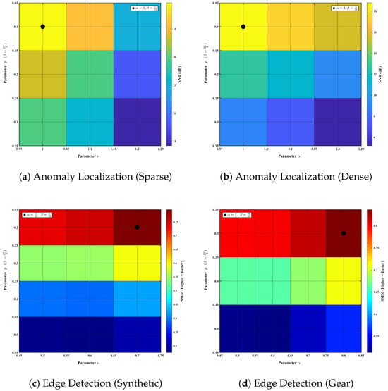
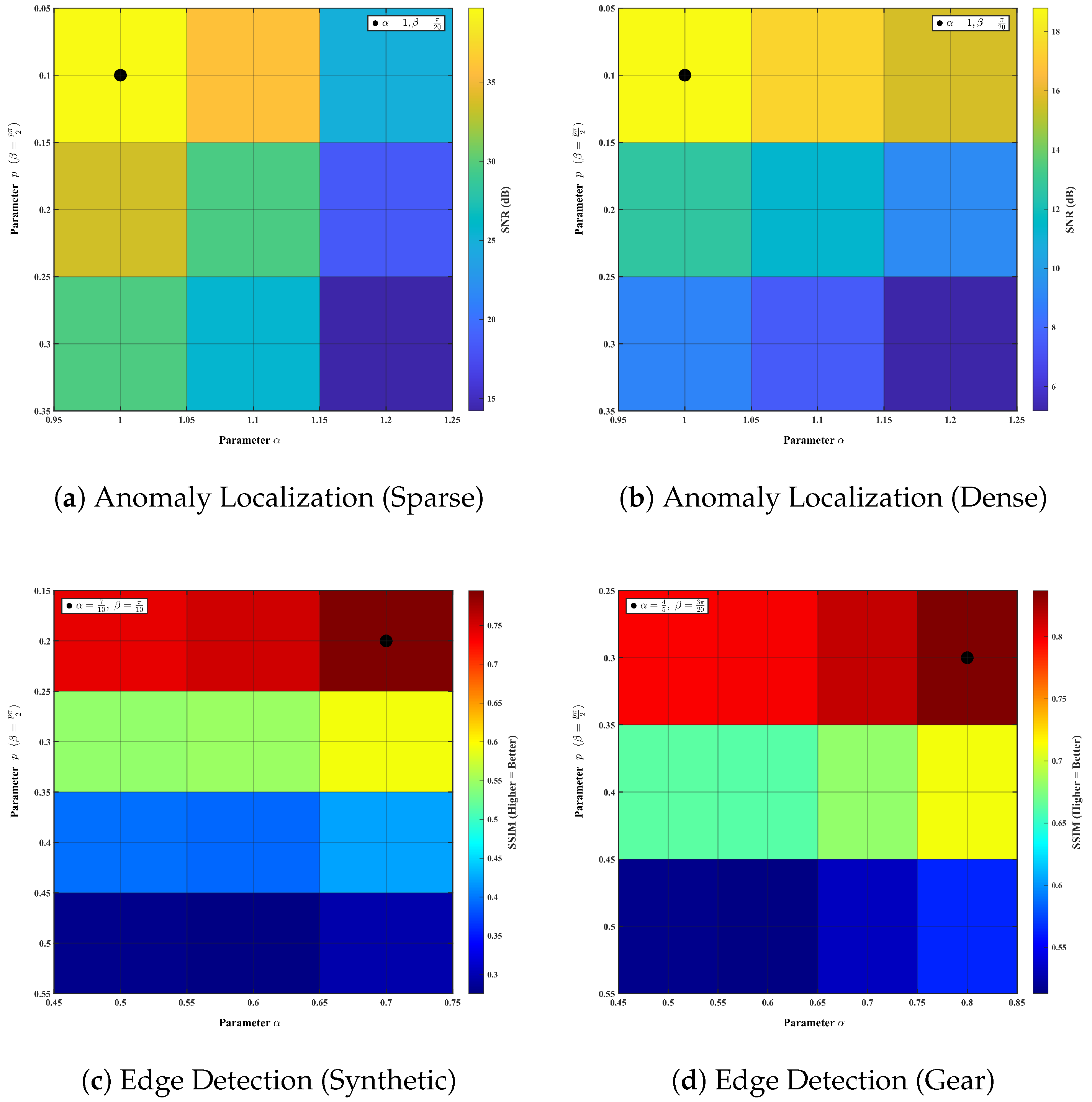
While the applications in Section 5.2, Section 5.3 and Section 5.4 utilize exhaustive grid searches or learnable parameters to automatically determine optimality, the tasks in Section 5.1 and Section 5.5 rely on empirical parameter selection. To rigorously validate the robustness of these empirically chosen parameters, we conducted a fine-grained sensitivity analysis, visualized in Figure 11. First, regarding the anomaly localization tasks (Section 5.1, Figure 11a,b): The sensitivity analysis confirmed that our initial estimates were near-optimal, identifying a refined setting $(\alpha =1,\beta ={\displaystyle \frac{\pi }{20}})$ that further maximized the performance gains reported in Table 3. Subsequently, for the edge detection task in this section (Figure 11c,d): The empirically selected parameters (marked with black dots) fall precisely within the high-performance regions (dark red zone) of the SSIM metric. This confirms that the empirical choices were well-founded and that the GFRHT performance is robust to small parameter variations within these regions.

Figure 11. Parameter sensitivity analysis verifying the robustness and optimality of GFRHT. (a,b) SNR performance for anomaly localization (Section 5.1). The fine-grained search identified an optimal peak at $(\alpha =1,p=0.1,\mathrm{i}.\mathrm{e}.,\beta ={\displaystyle \frac{\pi }{20}})$, which is used to update the results in Table 3, yielding significant performance gains over the initial estimates. (c,d) SSIM performance for edge detection (Section 5.5), confirming that the selected parameters (•) lie in the optimal region.

6. Discussions and Conclusions

6.1. Discussions

This paper introduces the GFRHT, a novel dual-parameter generalization of the conventional GHT. The GFRHT successfully overcomes the fundamental limitations of the GHT by enabling analysis in an arbitrary fractional domain via the order parameter $\alpha$, while the angle parameter $\beta$ allows for continuous phase shift adjustment and eliminates information loss at real eigenvalues.

The experimental results consistently validate the superiority of the GFRHT over the GHT across a diverse range of applications. For anomaly detection, the GFRHT exhibited remarkable robustness across varying graph densities and anomaly types, significantly outperforming the GHT in both sparse and dense graphs. Extending this validation from synthetic benchmarks to real-world data, experiments on the Molene Weather Dataset confirm the method’s ability to precisely localize anomalies. This consistency highlights its practical utility in scenarios where exact localization is critical. In speech classification, the fusion of features derived from the GFRHT with those from the classical DFRFT yielded state-of-the-art performance across diverse tasks. In edge detection, the GFRHT produced sharper and more continuous edges, particularly in complex image regions, by emphasizing features at optimal fractional scales. The consistent performance gains across data scales further attest to the robustness and generalizability of the proposed framework, underscoring the complementary and enriched representation provided by fractional analysis in both classical and graph domains.

6.2. Methodological Limitations and Future Directions

Despite the promising results, two main limitations of the current framework warrant attention to guide future research:

Methodological Limitations:

• The computational complexity of the GFRHT is significantly higher than that of the parameter-free GHT. Specifically, the GHT relies on a single eigen-decomposition, whereas the GFRHT requires two eigen-decompositions, which substantially increases its computational cost ($\mathcal{O}\left(N^3\right)$). This computational overhead currently restricts the direct application of GFRHT to massive-scale graphs.
• Regarding the experimental scope, while our study validates the method on both synthetic and real-world datasets (including sensor networks and speech signals), these scenarios predominantly involve static graph topologies. The generalizability and resilience of the method on more complex, noisy, and dynamic systems—such as time-varying graphs or multi-layer networks—remain to be fully explored.

Directions for Future Research: Future work will focus on addressing these limitations and exploring new frontiers:

• Scalability and fast algorithms: To mitigate the computational overhead, we will dedicate future efforts to researching and developing fast approximate algorithms specifically for the GFRFT and GFRHT. Instead of relying on full eigen-decompositions, we aim to investigate numerical methods or structural approximations that can accelerate the computation of the GFRFT matrix ${\mathbf{F}}^{\alpha }$, thereby enabling efficient processing of large-scale graphs.
• Dynamic graphs: We plan to extend the GFRHT to dynamic graph settings to handle temporally evolving structures, validating its performance on time-varying networks.
• Deep learning integration: We will explore the integration of the GFRHT as a learnable layer within Graph Neural Networks (GNNs) for end-to-end feature learning.
• Broader applications: We will investigate its applicability in other domains (e.g., bioacoustics, neuroimaging) to thoroughly assess its generalizability across complex real-world scenarios.

6.3. Conclusions

In conclusion, we propose and formalize the GFRHT, a flexible and powerful tool for graph signal processing that generalizes the conventional GHT through a principled dual-parameter framework. By enabling continuous interpolation between domains and tunable phase shifts, the GFRHT addresses the core limitations of the GHT and offers unprecedented control over graph signal analysis.

Theoretical properties such as linearity, shift-invariance, and invertibility provide a rigorous mathematical foundation for the GFRHT. Empirical evaluations in anomaly localization, speech classification and edge detection further verify its effectiveness, revealing significant and consistent performance improvements over the conventional GHT. With its adaptability and robustness, the proposed GFRHT emerges as a promising tool for a broad spectrum of graph-based inference tasks, encompassing computer vision, network analysis, and biomedical signal processing.

References

- Ortega, A.; Frossard, P.; Kovačević, J.; Moura, J.M.; Vandergheynst, P. Graph signal processing: Overview, challenges, and applications. Proc. IEEE 2018, 106, 808–828. [Google Scholar] [CrossRef] [Scilit]
- Ortega, A. Introduction to Graph Signal Processing; Cambridge University Press: Cambridge, UK, 2022. [Google Scholar]
- Djuric, P.; Richard, C. Cooperative and Graph Signal Processing: Principles and Applications; Academic Press: Cambridge, MA, USA, 2018. [Google Scholar]
- Liu, W.; Haardt, M.; Greco, M.S.; Mecklenbräuker, C.F.; Willett, P. Twenty-five years of sensor array and multichannel signal processing: A review of progress to date and potential research directions. IEEE Signal Process. Mag. 2023, 40, 80–91. [Google Scholar] [CrossRef] [Scilit]
- Jabłoński, I. Graph signal processing in applications to sensor networks, smart grids, and smart cities. IEEE Sens. J. 2017, 17, 7659–7666. [Google Scholar] [CrossRef] [Scilit]
- Huang, W.; Bolton, T.A.; Medaglia, J.D.; Bassett, D.S.; Ribeiro, A.; Van De Ville, D. A graph signal processing perspective on functional brain imaging. Proc. IEEE 2018, 106, 868–885. [Google Scholar] [CrossRef] [Scilit]
- Rui, L.; Nejati, H.; Cheung, N.M. Dimensionality reduction of brain imaging data using graph signal processing. In Proceedings of the 2016 IEEE International Conference on Image Processing (ICIP), Phoenix, AZ, USA, 25–28 September 2016; IEEE: Piscataway, NJ, USA, 2016; pp. 1329–1333. [Google Scholar]
- Ramakrishna, R.; Scaglione, A. Grid-graph signal processing (grid-GSP): A graph signal processing framework for the power grid. IEEE Trans. Signal Process. 2021, 69, 2725–2739. [Google Scholar] [CrossRef] [Scilit]
- Giannakis, G.B.; Kekatos, V.; Gatsis, N.; Kim, S.J.; Zhu, H.; Wollenberg, B.F. Monitoring and optimization for power grids: A signal processing perspective. IEEE Signal Process. Mag. 2013, 30, 107–128. [Google Scholar] [CrossRef] [Scilit]
- Ramakrishna, R.; Scaglione, A. Detection of false data injection attack using graph signal processing for the power grid. In Proceedings of the 2019 IEEE Global Conference on Signal and Information Processing (GlobalSIP), Ottawa, ON, Canada, 11–14 November 2019; IEEE: Piscataway, NJ, USA, 2019; pp. 1–5. [Google Scholar]
- Stankovic, L.; Mandic, D.; Dakovic, M.; Brajovic, M.; Scalzo, B.; Constantinides, T. Graph signal processing–Part I: Graphs, graph spectra, and spectral clustering. arXiv 2019, arXiv:1907.03467. [Google Scholar]
- Shi, J.; Moura, J.M. Graph signal processing: Dualizing GSP sampling in the vertex and spectral domains. IEEE Trans. Signal Process. 2022, 70, 2883–2898. [Google Scholar] [CrossRef] [Scilit]
- Gavili, A.; Zhang, X.P. On the shift operator, graph frequency, and optimal filtering in graph signal processing. IEEE Trans. Signal Process. 2017, 65, 6303–6318. [Google Scholar] [CrossRef] [Scilit]
- Venkitaraman, A.; Chatterjee, S.; Handel, P. On Hilbert transform of signals on graphs. In Proceedings of the 11th International Conference on Sampling Theory and Applications, Washington, DC, USA, 25–29 May 2015. [Google Scholar]
- Venkitaraman, A.; Chatterjee, S.; Handel, P. On Hilbert transform, analytic signal, and modulation analysis for signals over graphs. Signal Process. 2019, 156, 106–115. [Google Scholar] [CrossRef] [Scilit]
- Lu, K.S.; Ortega, A. Fast graph Fourier transforms based on graph symmetry and bipartition. IEEE Trans. Signal Process. 2019, 67, 4855–4869. [Google Scholar] [CrossRef] [Scilit]
- Domingos, J.; Moura, J.M. Graph Fourier transform: A stable approximation. IEEE Trans. Signal Process. 2020, 68, 4422–4437. [Google Scholar] [CrossRef] [Scilit]
- Patanè, G. Fourier-based and rational graph filters for spectral processing. IEEE Trans. Pattern Anal. Mach. Intell. 2022, 45, 7063–7074. [Google Scholar] [CrossRef] [Scilit] [PubMed]
- Shang, Y. Vulnerability of networks: Fractional percolation on random graphs. Phys. Rev. E. 2014, 89, 012813. [Google Scholar] [CrossRef] [Scilit]
- Shang, Y. The fractional chromatic number of random graphs. Discret. Math. 2026, 349, 114962. [Google Scholar] [CrossRef] [Scilit]
- Wang, Y.Q.; Li, B.Z. The fractional Fourier transform on graphs: Sampling and recovery. In Proceedings of the 2018 14th IEEE International Conference on Signal Processing (ICSP), Beijing, China, 12–16 August 2018; IEEE: Piscataway, NJ, USA, 2018; pp. 1103–1108. [Google Scholar]
- Ozaktas, H.M.; Mendlovic, D. Fractional Fourier transforms and their optical implementation. II. J. Opt. Soc. Am. A 1993, 10, 2522–2531. [Google Scholar] [CrossRef] [Scilit]
- Pei, S.C.; Ding, J.J. Fractional Fourier transform, Wigner distribution, and filter design for stationary and nonstationary random processes. IEEE Trans. Signal Process. 2010, 58, 4079–4092. [Google Scholar] [CrossRef] [Scilit]
- Wu, J.M.; Jiang, S.; Lu, M.F.; Fan, J.F.; Li, Y.F.; Ji, Y.; Zhang, F.; Tao, R. Improved fractional Fourier transform method based on triangle shrinkage for estimating physical parameters from Newton’s rings. Opt. Laser Technol. 2024, 176, 110887. [Google Scholar] [CrossRef] [Scilit]
- Wei, D.Y. Novel convolution and correlation theorems for the fractional Fourier transform. Optik 2016, 127, 3669–3675. [Google Scholar] [CrossRef] [Scilit]
- Yang, Y.X.; Tao, R.; Wei, K.X.; Shi, J. Single-shot phase retrieval from a fractional Fourier transform perspective. IEEE Trans. Signal Process. 2024, 72, 3303–3317. [Google Scholar] [CrossRef] [Scilit]
- Yan, F.J.; Li, B.Z. Windowed fractional Fourier transform on graphs: Properties and fast algorithm. Digit. Signal Process. 2021, 118, 103210. [Google Scholar] [CrossRef] [Scilit]
- Alikaşifoğlu, T.; Kartal, B.; Koç, A. Wiener filtering in joint time-vertex fractional Fourier domains. IEEE Signal Process. Lett. 2024, 31, 1319–1323. [Google Scholar] [CrossRef] [Scilit]
- Alikaşifoğlu, T.; Kartal, B.; Özgünay, E.; Koç, A. Joint time-vertex fractional Fourier transform. Signal Process. 2025, 233, 109944. [Google Scholar] [CrossRef] [Scilit]
- Gan, Y.C.; Chen, J.Y.; Li, B.Z. The windowed two-dimensional graph fractional Fourier transform. Digit. Signal Process. 2025, 162, 105191. [Google Scholar] [CrossRef] [Scilit]
- Shang, L.B.; Zhang, Z.C. Frames and vertex-frequency representations in graph fractional Fourier domain. Signal Process. 2025, 238, 110198. [Google Scholar] [CrossRef] [Scilit]
- Alikaşifoğlu, T.; Kartal, B.; Koç, A. Graph fractional Fourier transform: A unified theory. IEEE Trans. Signal Process. 2024, 72, 3834–3850. [Google Scholar] [CrossRef] [Scilit]
- Chen, J.Y.; Zhang, Y.; Li, B.Z. Graph linear canonical transform: Definition, vertex-frequency analysis and filter design. IEEE Trans. Signal Process. 2024, 72, 5691–5707. [Google Scholar] [CrossRef] [Scilit]
- Yan, F.J.; Li, B.Z. Multi-dimensional graph fractional Fourier transform and its application to data compression. Digit. Signal Process. 2022, 129, 103683. [Google Scholar] [CrossRef] [Scilit]
- Li, N.; Zhang, Z.C. Multi-dimensional graph linear canonical transform. Digit. Signal Process. 2025, 165, 105334. [Google Scholar] [CrossRef] [Scilit]
- Cui, M.J.; Zhang, Z.C.; Yao, W. Multiple-Parameter Graph Fractional Fourier Transform: Theory and Applications. arXiv 2025, arXiv:2507.23570. [Google Scholar] [CrossRef] [Scilit]
- Bianchi, F.M.; Grattarola, D.; Livi, L.; Alippi, C. Graph neural networks with convolutional arma filters. IEEE Trans. Pattern Anal. Mach. Intell. 2021, 44, 3496–3507. [Google Scholar] [CrossRef] [Scilit]
- Salim, A.; Sumitra, S. Spectral graph convolutional neural networks in the context of regularization theory. IEEE Trans. Neural Netw. Learn. Syst. 2022, 35, 4373–4384. [Google Scholar] [CrossRef] [Scilit]
- Airani, R.; Kamble, S. Spectral approximation of Gaussian random graph Laplacians and applications to pattern recognition. Pattern Recognit. 2025, 164, 111555. [Google Scholar] [CrossRef] [Scilit]
- Yan, Z.Q.; Zhang, Z.C. Trainable Joint Time-Vertex Fractional Fourier Transform. arXiv 2025, arXiv:2507.21527. [Google Scholar] [CrossRef] [Scilit]
- Sheng, C.J.; Zhang, Z.C.; Yao, W. Graph Embedding in the Graph Fractional Fourier Transform Domain. arXiv 2025, arXiv:2508.02383. [Google Scholar] [CrossRef] [Scilit]
- Pei, S.C.; Yeh, M.H. Discrete fractional Hilbert transform. IEEE Trans. Circuits Syst. II Analog Digit. Signal Process. 2000, 47, 1307–1311. [Google Scholar]
- Hammond, D.K.; Vandergheynst, P.; Gribonval, R. Wavelets on graphs via spectral graph theory. Appl. Comput. Harmon. Anal. 2011, 30, 129–150. [Google Scholar] [CrossRef] [Scilit]
- Perraudin, N.; Paratte, J.; Shuman, D.; Martin, L.; Kalofolias, V.; Vandergheynst, P.; Hammond, D.K. GSPBOX: A toolbox for signal processing on graphs. arXiv 2014, arXiv:1408.5781. [Google Scholar]
- Perraudin, N.; Vandergheynst, P. Stationary signal processing on graphs. IEEE Trans. Signal Process. 2017, 65, 3462–3477. [Google Scholar] [CrossRef] [Scilit]
Disclaimer/Publisher’s Note: The statements, opinions and data contained in all publications are solely those of the individual author(s) and contributor(s) and not of MDPI and/or the editor(s). MDPI and/or the editor(s) disclaim responsibility for any injury to people or property resulting from any ideas, methods, instructions or products referred to in the content. |
© 2026 by the authors. Licensee MDPI, Basel, Switzerland. This article is an open access article distributed under the terms and conditions of the Creative Commons Attribution (CC BY) license.