


Abstract
This paper presents a systematic comparative analysis of rational approximation methods for fractional-order systems, which are widely used to describe dynamics with memory and hereditary effects. Since fractional-order operators generally lead to irrational transfer functions, rational approximations are required for practical simulation, analysis, and implementation. Seven approximation methods are investigated, including Classical Oustaloup, Refined Oustaloup, Continued Fraction Expansion (CFE), Curve Fitting, Modified Stability Boundary Locus (M-SBL), Equal-Ripple, and Exact-Phase methods. The methods are evaluated using three representative test cases: a fundamental fractional-order operator, a higher-order fractional-order transfer function, and a fractional-order controller. Both frequency-domain characteristics and time-domain responses are examined using magnitude and phase RMSE, step-response RMSE, IAE, and ISE. The results show that approximation performance depends on both the approximation method and the type of fractional-order system. Refined Oustaloup generally provides close agreement with the reference model for the fundamental operator and higher-order transfer function, while the controller results show a different performance across the evaluated metrics. The findings demonstrate that no single method is universally optimalm and that both frequency- and time-domain evaluations are important for assessing rational approximation accuracy.
1. Introduction
Fractional calculus extends classical differentiation and integration to non-integer orders [1,2] and provides a useful framework for describing systems with memory, hereditary effects, and frequency-dependent dynamics [3,4]. Its application has received increasing attention in control engineering and system modeling, particularly for physical processes whose dynamics cannot be adequately represented by conventional integer-order models. Examples include viscoelastic materials, diffusion processes, electrochemical systems, and other systems with memory-dependent behavior [1].
Beyond its applications in system modeling and control, fractional calculus has also gained attention in approximation theory. Recent studies have investigated fractional operators and their approximation properties, contributing to the development of approximation techniques within this mathematical field [5,6]. These investigations further illustrate the expanding scope of fractional calculus and its relevance to different areas of mathematical research.
A basic element of fractional-order modeling is the fractional-order operator , where α is a real-valued order [7]. Such operators generally lead to irrational transfer functions, and therefore cannot be directly represented by finite-dimensional rational models [2]. In practical applications, rational approximations are commonly used to enable numerical simulation, system analysis, controller implementation, and experimental realization [8]. The accuracy of these approximations is consequently important, because deviations introduced during the approximation can affect the subsequent analysis and control design [4,9].
A variety of rational approximation methods have been developed, including the Oustaloup Recursive Approximation, Refined Oustaloup Approximation, Continued Fraction Expansion, Modified Stability Boundary Locus (M-SBL), the Curve Fitting method, and Equal-Ripple and Exact-Phase approaches [4,10]. These methods are based on different approximation principles, and can therefore produce different levels of accuracy and model complexity. Although increasing the approximation order can improve the representation of fractional-order dynamics over a selected frequency range, it also increases the complexity of the resulting rational model. The choice of an approximation method, therefore, involves a balance between representation accuracy and model complexity [7,10,11].
An important issue is that the performance of an approximation method may depend on the fractional-order system being considered. A method that performs well for an individual fractional operator may behave differently when applied to a higher-order fractional-order transfer function or a fractional-order controller [4,12]. In addition, good agreement in the frequency domain does not necessarily imply the same level of agreement in the time domain. A comparison that considers different system structures together with both frequency- and time-domain behavior can, therefore, provide a more complete view of the practical performance of rational approximation methods [7].
In this study, seven rational approximation methods are systematically compared using three representative fractional-order test cases: the fundamental fractional-order operator s0.5, a higher-order fractional-order transfer function, and a fractional-order controller. The methods are evaluated under consistent simulation conditions, using both frequency- and time-domain analyses. Bode responses and magnitude and phase errors are used to assess frequency-domain accuracy, while step responses, together with RMSE, IAE, and ISE, are used to evaluate time-domain agreement. The effect of approximation order is also examined for the fundamental fractional-order operator.
The main contributions of this study are the following:
- A systematic comparison of seven rational approximation methods under a common simulation and evaluation framework.
- Evaluation across three fractional-order test cases, ranging from a fundamental fractional operator to a higher-order transfer function and a fractional-order controller.
- Combined frequency- and time-domain evaluation using Bode responses, step responses, and quantitative error measures.
- Investigation of approximation-order effects to examine the relationship between approximation accuracy and model complexity.
- Comparative analysis of the obtained results to highlight differences in approximation behavior across different fractional-order systems.
The paper is structured as follows: Section 2 presents the rational approximation techniques examined in this study. Section 3 presents the selected test systems, simulation settings, and performance evaluation metrics. Section 4 presents and discusses the frequency- and time-domain results for the three test systems. The paper closes in Section 5, with a discussion of the principal findings and possible future research directions.
2. Rational Approximation Methods for Fractional-Order Systems
Fractional-order operators generally result in irrational transfer functions, which makes their direct numerical realization difficult [2]. Rational approximation methods provide finite-dimensional representations that can be used for simulation, analysis, and implementation of fractional-order systems [7]. The methods selected for this investigation are outlined in this section, covering both recursive and analytical approaches. The main principles and mathematical formulations of each method are briefly described, to provide a common basis for the comparative analysis presented in the subsequent sections.
2.1. Oustaloup Recursive Approximation
The Oustaloup Recursive Approximation (ORA) is one of the most widely used methods for the rational approximation of fractional-order operators in control engineering. It provides a finite-dimensional integer-order transfer function that closely reproduces the frequency-response characteristics of the fractional-order operator sα over a specified frequency interval. Owing to its good accuracy and tunable structure, the Oustaloup method has become a standard tool for the practical realization of fractional-order controllers and systems [8,13,14].
The Oustaloup method approximates the fractional-order operator sα using a rational transfer function defined over a limited frequency band, expressed as follows:
where N represents the approximation parameter, [ωb, ωh] represents the selected frequency interval, K is a constant gain factor and ωi and represent the pole and zero frequencies, respectively. In the classical Oustaloup formulation, the approximation is constructed using 2N + 1 pole-zero pairs. Consequently, the resulting rational transfer function has a numerator and denominator degree of 2N + 1. Thus, N represents the approximation parameter, rather than the actual degree of the rational model.
The parameters of the approximation are computed according to the following formulas:
where α is the fractional order, ωb and ωh are the lower and upper bounds of the approximation frequency range, and N determines the balance between approximation precision and model complexity [15].
The Oustaloup technique retains the essential frequency-domain characteristics of the ideal fractional-order operator. In particular, it provides an approximately constant phase shift equal to and a magnitude slope of 20α dB/decade, within the design frequency band. These properties make the method especially suitable for frequency-domain control design.
However, the accuracy of the approximation depends strongly on the selected approximation order and frequency range. Recent studies have shown that different Oustaloup variants and parameter choices may lead to significantly different time- and frequency-domain responses, which motivates the careful selection of approximation parameters and the comparative analysis performed in this paper [16,17].
- Worked Example: Third-Order Oustaloup Approximation of s0.5
To illustrate the construction of the Oustaloup approximation, consider the fractional operator s0.5 over the frequency range ω ∈ [ωb,ωh] = [0.01, 100] rad/s. An approximation parameter of (N = 1) is selected, resulting in a third-order rational transfer function with three poles and three zeros. The frequency ratio and gain are calculated using the corresponding approximation formulas. The resulting pole and zero locations are summarized in Table 1.
Table 1.
Poles and Zeros of the Third-Order Oustaloup Approximation for s0.5 (ωb = 0.01 rad/s, ωh = 100 rad/s, N = 1).
Using these values, the rational approximation of s0.5 is constructed as
This transfer function represents a third-order integer-order approximation of the fractional operator s0.5 that accurately reproduces its magnitude and phase behavior within the frequency band [0.01, 100] rad/s. This model is subsequently used in the simulation and comparative analysis presented in the following sections.
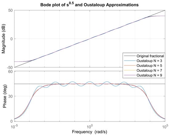
Figure 1 presents a comparison of the Bode magnitude and phase characteristics of the reference fractional-order operator s0.5 and its rational approximations obtained using the Oustaloup Recursive method for different approximation orders (N = 3, 5, 7 and 9).
Figure 1.
Frequency-domain comparison of the fractional-order operator s0.5 and its Oustaloup rational approximations for (N = 3, 5, 7,) and (9), corresponding to seventh-, eleventh-, fifteenth-, and nineteenth-order rational models, respectively, over the selected frequency interval.
As the approximation order increases, the rational approximation exhibits a progressively improved agreement with the reference fractional response across the specified frequency band. In particular, higher-order approximations provide a more accurate representation of both magnitude slope and phase angle, especially in the mid-frequency region.
Conversely, lower-order approximations show noticeable deviations near the lower- and upper-boundary frequencies, reflecting the inherent trade-off between approximation accuracy and model order. These results illustrate that increasing the approximation order enhances fidelity to the fractional dynamics at the expense of increased computational and structural complexity.
2.2. Refined Oustaloup Recursive Approximation
The classical Oustaloup Recursive Approximation provides an efficient rational approximation of the fractional-order operator sα over a predefined frequency band. However, it is well known that the approximation accuracy deteriorates near the lower- and upper-boundary frequencies of the selected interval. This limitation leads to noticeable deviations in both magnitude and phase characteristics near the boundaries of the frequency interval of interest.
To overcome this drawback, Xue, Zhao, and Chen [18] proposed a modified version of the Oustaloup Approximation, commonly referred to as the Refined (or modified) Oustaloup Approximation method. The primary aim of this modification is to improve the fitting quality over the entire frequency band, with particular emphasis on reducing the boundary errors [19].
In the Refined Oustaloup method, the fractional operator sα is approximated by the following rational transfer function:
where N represents the approximation order, ωl and ωh represent the lower- and upper-bound frequencies, respectively, and b and d are design parameters introduced to enhance the approximation performance.
The gain factor K and the pole–zero frequencies are defined as
Through extensive numerical analysis, Xue et al. reported that the choice b = 10 and d = 9 [18] yields near-optimal fitting performance for a wide range of fractional orders and frequency bands. Compared to the classical Oustaloup approximation, the Refined method provides a significantly improved matching of both magnitude and phase characteristics, particularly near the boundary frequencies.
As a result, the Refined Oustaloup approximation has become a widely adopted method for accurately representing fractional-order operators in control design and simulation studies.
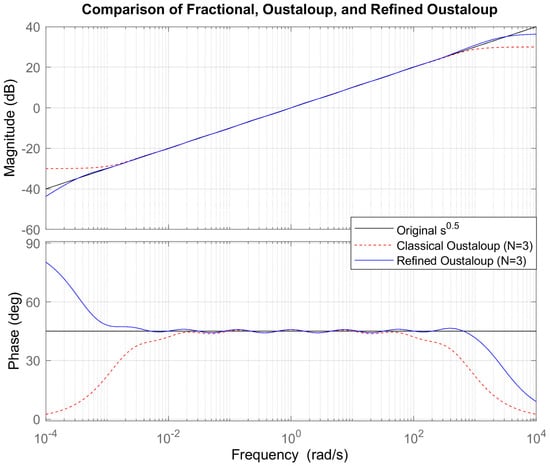
Figure 2 shows that, in the mid-frequency region, both approximation methods provide a close match to the reference fractional response, indicating that the recursive structure is effective in reproducing the desired slope and phase behavior. However, noticeable differences appear near the lower- and upper-boundary frequencies of the approximation interval.
Figure 2.
Bode diagrams comparing the magnitude and phase responses of the fractional-order operator s0.5 with the Classical and Refined Oustaloup approximations, using ωb = 0.001, ωh = 1000, and N = 3.
In particular, the classical Oustaloup approximation exhibits increasing deviations in both magnitude and phase as the frequency approaches the band limits. These boundary errors are a well-known drawback of the classical method, and may lead to inaccurate system representation in practical control applications. In contrast, the Refined Oustaloup approximation maintains a significantly closer agreement with the reference fractional operator over the entire frequency range, especially near the boundary frequencies.
This improvement confirms the fact that the additional correction term and the optimized parameter selection b = 10 and d = 9 effectively reduce edge distortions. Consequently, the Refined Oustaloup method provides a more reliable and accurate rational approximation of fractional-order operators, making it better suited for high-fidelity modeling and control design over a finite frequency band.
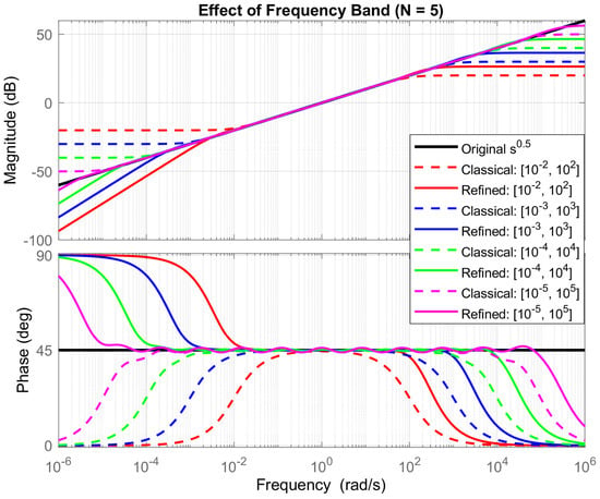
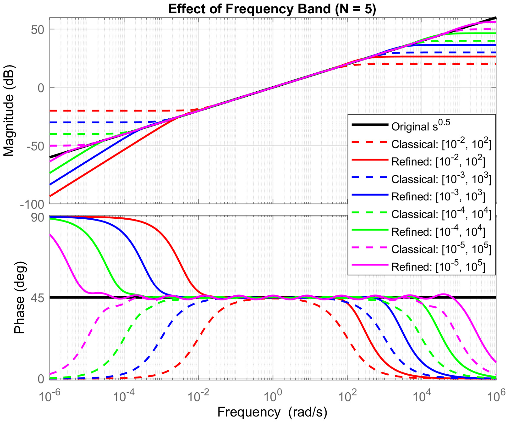
Figure 3 illustrates that, for all considered cases, both approximation methods provide a good match to the reference fractional response in the central region of the selected frequency band. However, the quality of the approximation strongly depends on the chosen boundary frequencies. When a narrower frequency interval is selected, the approximation accuracy is high within this limited range, but deteriorates rapidly outside the designed band. Conversely, as the frequency band is widened, the approximation is distributed over a larger interval, leading to increased deviations near the new boundary frequencies.
Figure 3.
Bode diagrams comparing the magnitude and phase characteristics of the Classical and Refined Oustaloup approximations at N = 5 across different approximation frequency bands.
A clear difference between the two methods is observed at the band limits. The classical Oustaloup approximation exhibits pronounced magnitude and phase distortions near ωb and ωh, and these distortions become more significant as the frequency range is extended. In contrast, the Refined Oustaloup approximation preserves a closer agreement with the reference fractional operator for all considered frequency bands, particularly near the lower and upper boundaries.
These results highlight the fact that the selection of the approximation frequency range is a critical design parameter, and directly influences the fidelity of the rational approximation.
Moreover, the Refined Oustaloup method demonstrates superior robustness with respect to frequency-band variation, making it more suitable for applications requiring accurate fractional-order modeling over wide frequency intervals.
2.3. Continued Fraction Expansion (CFE) Method
The Continued Fraction Expansion (CFE) method is a classical algebraic technique for constructing rational approximations of fractional-order operators. In contrast to methods that rely on frequency-domain approximation, such as the Oustaloup recursive technique, the CFE method is derived from the algebraic expansion of a generating function, and yields low-order rational transfer functions with simple pole–zero structures. Due to its low computational complexity and ease of implementation, the CFE method has been widely used in the simulation and realization of fractional-order integrators and differentiators.
The starting point of the CFE method is the binomial expression (1 + x)α, which can be expanded into a continued fraction form. This representation allows the construction of a sequence of rational approximations by truncating the continued fraction after a finite number of terms. The continued fraction expansion of (1 + x)α can be written as [4,14]
By truncating this continued fraction after a finite number of terms, a rational approximation of finite order is obtained. Retaining only the first two terms yields the first-order truncated approximation:
After algebraic simplification, this expression becomes
where denotes the neglected higher-order terms.
To obtain an approximation of the fractional operator sα, the variable substitution
is introduced, where s denotes the Laplace variable. Substituting (10) into (11) yields a first-order rational approximation of sα in the form
Higher-order approximations are obtained by retaining more terms in the continued fraction expansion. CFE approximations of sα, with orders ranging from first to fourth, are summarized in Table 2 [20].
Table 2.
First- to fourth-order CFE approximations of sα.
For the particular case α = 0.5, which is widely used as a benchmark in fractional-order control, the low-order CFE approximations are shown in Table 3. As the approximation order increases, the number of poles and zeros increases symmetrically, which improves the approximation accuracy, at the expense of increased model complexity.
Table 3.
CFE approximations of s0.5 with orders ranging from first to fourth.
To quantify the usable frequency interval of each approximation, the effective frequency range is defined based on a prescribed magnitude error tolerance. Let GCFE(jω) denote the frequency response of a CFE approximation and ∣sα∣ = ωα the magnitude of the ideal fractional operator. The magnitude error in decibels is defined as
The effective frequency limits ωmin and ωmax are defined as the frequencies for which
and the corresponding bandwidth is given by B = ωmax − ωmin.
In this paper, the effective frequency ranges of the first- to fourth-order CFE approximations are obtained numerically, by evaluating (13) over a logarithmically spaced frequency grid and identifying the largest contiguous interval satisfying the tolerance condition. The resulting bandwidths are reported in Table 4.
Table 4.
Effective frequency ranges for CFE model of s0.5 within ±0.01 dB tolerance.
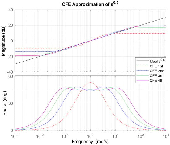
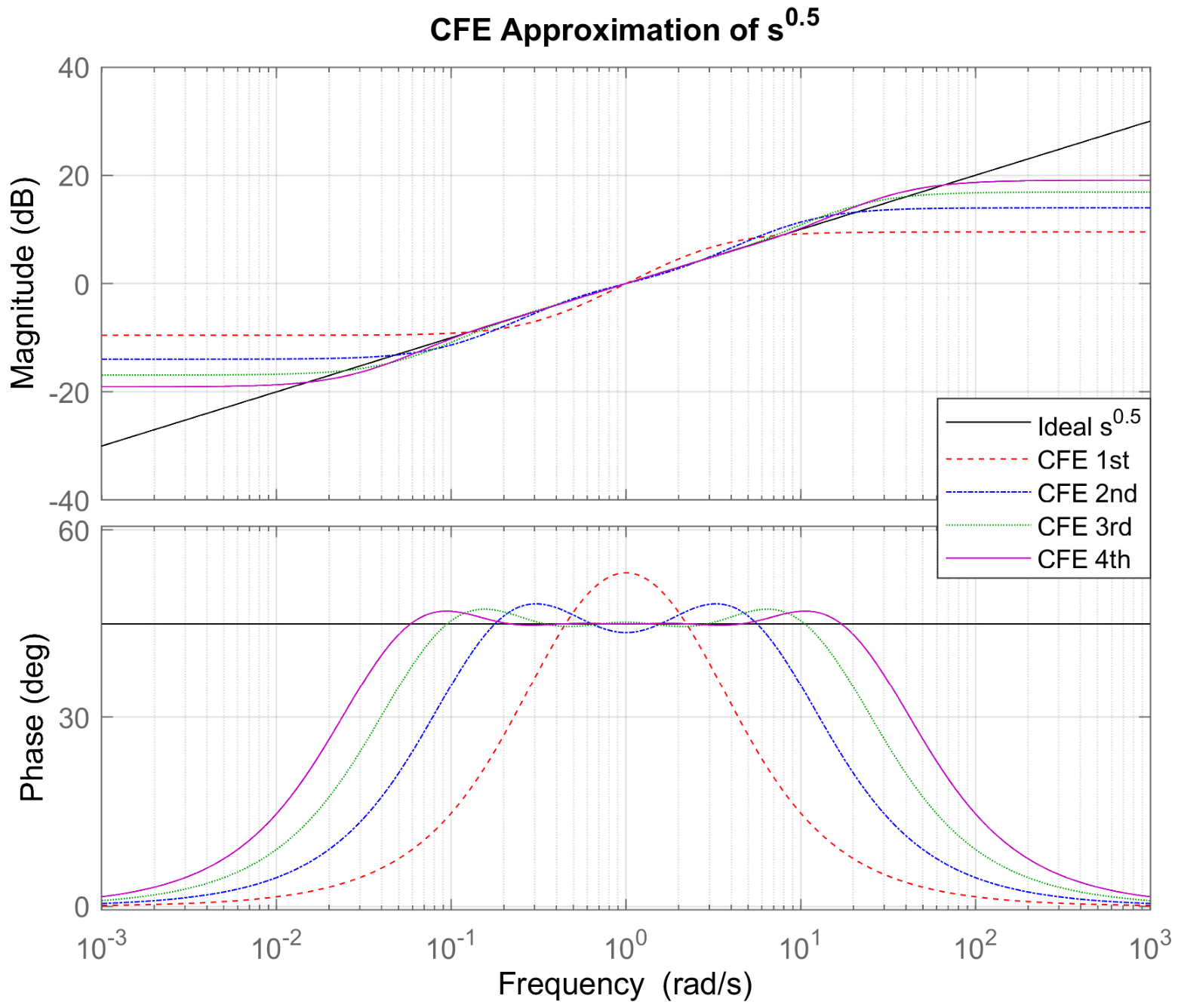
Figure 4 compares the frequency responses of the reference fractional operator s0.5 and its first- to fourth-order CFE approximations. As the approximation order increases, the magnitude and phase responses of the rational models approach more closely the reference fractional behavior over a wider frequency interval. The first-order model exhibits noticeable deviations outside a narrow band around the center frequency, while the third- and fourth-order models achieve accurate magnitude and phase agreement across a considerably wider frequency range. These observations are consistent with the effective bandwidth results reported in Table 4, and confirm the strong dependence of approximation accuracy on the model order.
Figure 4.
Bode diagram illustrating the magnitude and phase characteristics of the reference fractional operator s0.5 and its first- to fourth-order continued fraction expansion approximations.
2.4. Curve Fitting-Based Approximation Method
The Curve Fitting-Based approximation method is a frequency-domain approach for obtaining integer-order rational approximations of fractional-order operators. The method constructs the approximation directly from the exact frequency response of the fractional operator, avoiding predefined pole–zero distributions and recursive structures. This approach has been shown to provide high approximation accuracy over a specified frequency range when compared to classical approximation methods [21].
The first step in this process involves obtaining the frequency response data (FRD) for the fractional operator sα. This is achieved by substituting the Laplace operator with its frequency-domain equivalent, s = jω, and evaluating the function at logarithmically spaced frequency points within the desired range [ωL, ωH]:
To transform this data into a usable integer-order model, the method employs the Sanathanan–Koerner (SK) least-squares iterative approach [22]. The objective is to identify the coefficients of a transfer function defined as
where N represents the chosen order of approximation. The coefficients are adjusted by minimizing the discrepancy between the measured data points H(jω) and the model response G(jω), through a linearized objective function:
In this formulation, r represents the iteration step. Qr−1(jωk) is the denominator polynomial obtained from the previous iteration. The iteration proceeds until convergence, defined as
This iterative process ensures numerical robustness and improved convergence, compared to direct least-squares fitting.
Once the optimal coefficients are obtained, the rational approximation is realized in state-space form as
along with its associated transfer function
Common pole–zero cancellations are subsequently performed, to obtain a minimal realization suitable for simulation and controller implementation.
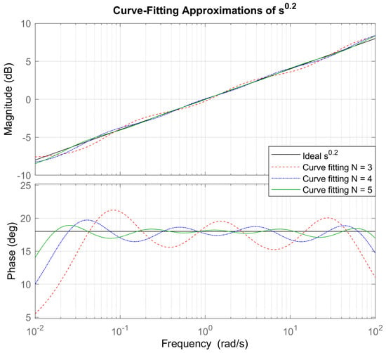
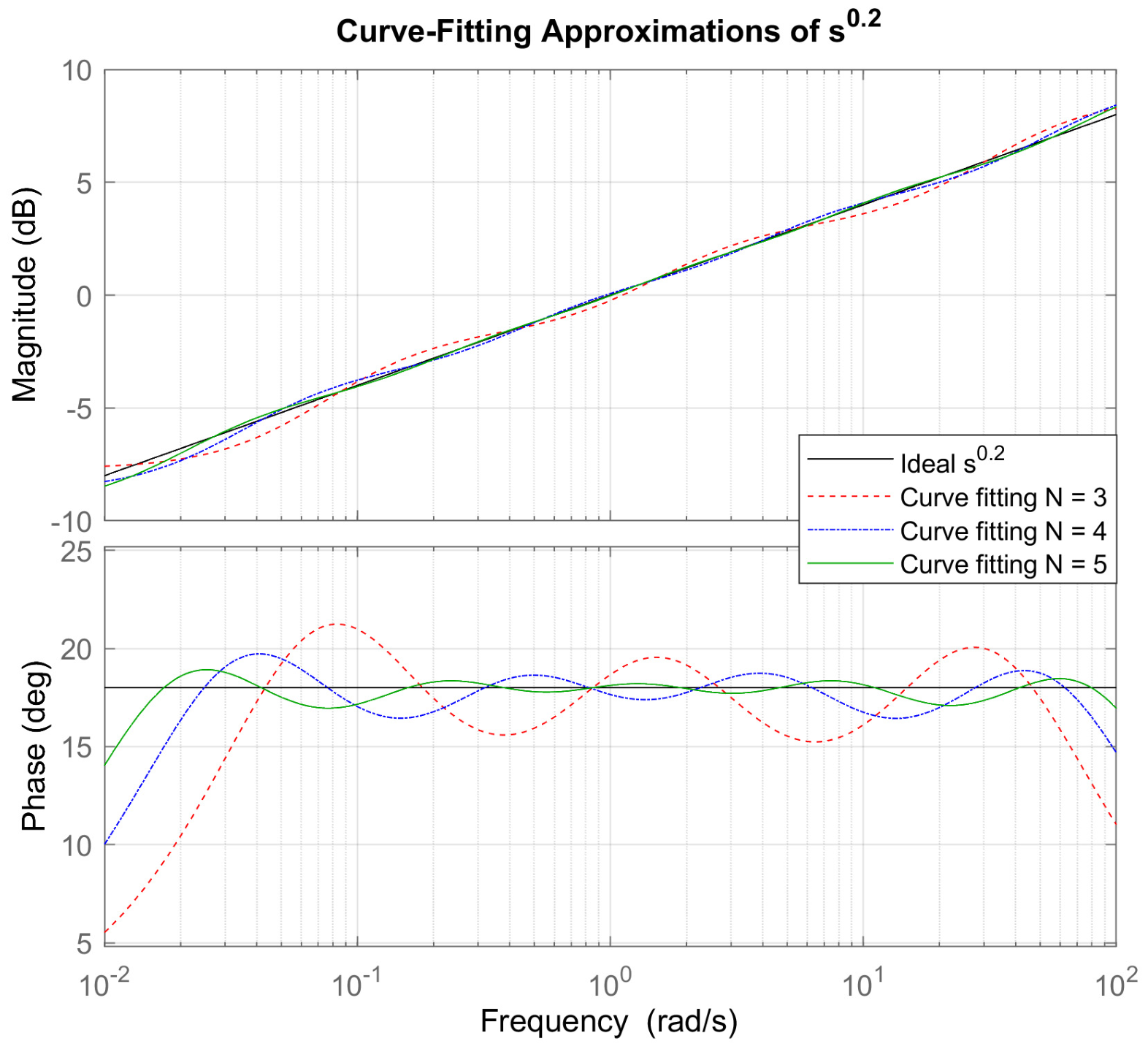
To demonstrate the proposed approach, a fractional-order differentiator of order s0.2 is considered. The desired frequency range ω is selected as (10−2, 102). Furthermore, to investigate the effect of the approximation order, the number of approximation terms N is chosen as 3, 4, and 5. The resulting transfer functions obtained from the implementation of the proposed method are listed in Table 5.
Table 5.
Third-, Fourth-, and Fifth-order Curve Fitting-Based Approximation Transfer Functions of s0.2.
Figure 5 presents magnitude and phase characteristics in the Bode diagram of the reference fractional-order differentiator s0.2 together with its Curve Fitting-Based rational approximations for approximation orders N = 3, 4 and 5. The results show that higher approximation orders lead to substantially better agreement in both magnitude and phase matching over the frequency range 10−2 to 102 rad/s, with the N = 5 exhibiting the closest agreement with the reference fractional behavior.
Figure 5.
Magnitude and phase characteristics in the Bode diagram of the reference fractional-order differentiator s0.2 and its Curve Fitting-Based rational approximations for approximation orders N = 3, 4 and 5, over the frequency range 10−2 to −102 rad/s.
2.5. Modified Stability Boundary Locus (M-SBL) Method
The Stability Boundary Locus (SBL) method was originally developed as a frequency-domain tool for analyzing the stability regions of fractional-order control systems. The fundamental idea of SBL is based on examining the system characteristic equation along the imaginary axis, and determining the parameter values at which the system transitions between stability and instability. While the original SBL concept is primarily used for stability analysis, it can also be exploited to construct integer-order approximations of fractional-order operators [23].
However, it has been observed that approximations obtained using the classical SBL approach may suffer from limited accuracy, and may not consistently reproduce fractional-order behavior with sufficient accuracy across an extended frequency interval. To overcome these limitations, the Modified Stability Boundary Locus (M-SBL) approximation method was proposed [4,24]. The key motivation behind M-SBL is to retain the stability-preserving property of the SBL approach, while improving the approximation accuracy by modifying the formulation of the rational approximation problem.
The Modified Stability Boundary Locus (M-SBL) method approximates the fractional-order operator sα, 0 < α < 1, by constructing a stable integer-order rational transfer function whose coefficients are obtained from stability boundary conditions evaluated at selected frequency points.
In the frequency domain, the fractional-order operator is expressed as
The objective of the M-SBL method is to approximate sα by an integer-order transfer function
where the numerator and denominator coefficients are arranged symmetrically, to guarantee stability and solve real and imaginary equations together, for n sampling points.
A logarithmically spaced frequency grid is defined over the approximation band
For an approximation order n, the frequency points are chosen as
These points define the stability boundary locus used for coefficient computation.
At each frequency point ωk, the approximation is enforced by equating the real and imaginary components of the characteristic equation. This leads to a linear system
where the matrix elements of are defined as
and the vector is given by
Solving the linear system yields the coefficient vector
from which the numerator polynomial is formed as
and the denominator polynomial is obtained by coefficient reversal,
Thus, the M-SBL approximation transfer function is finally written as
The denominator polynomial is obtained by coefficient reversal, as defined in (25). However, this structural arrangement alone does not guarantee Hurwitz stability. Therefore, the stability of the resulting M-SBL approximation should be verified by examining the locations of its poles. A stable approximation requires all poles to have negative real parts.
The approximation accuracy depends on the order n and the selected frequency range [ωl, ωh]. Increasing the order improves frequency-domain matching, at the cost of increased model complexity. The resulting transfer functions obtained from the implementation of M-SBL fitting method are listed in Table 6.
Table 6.
First-, second-, third-, fourth- and fifth-order M-SBL fitting model transfer functions of s0.3 in ωk ∈ [0.1,10] rad/s.
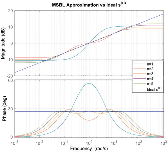
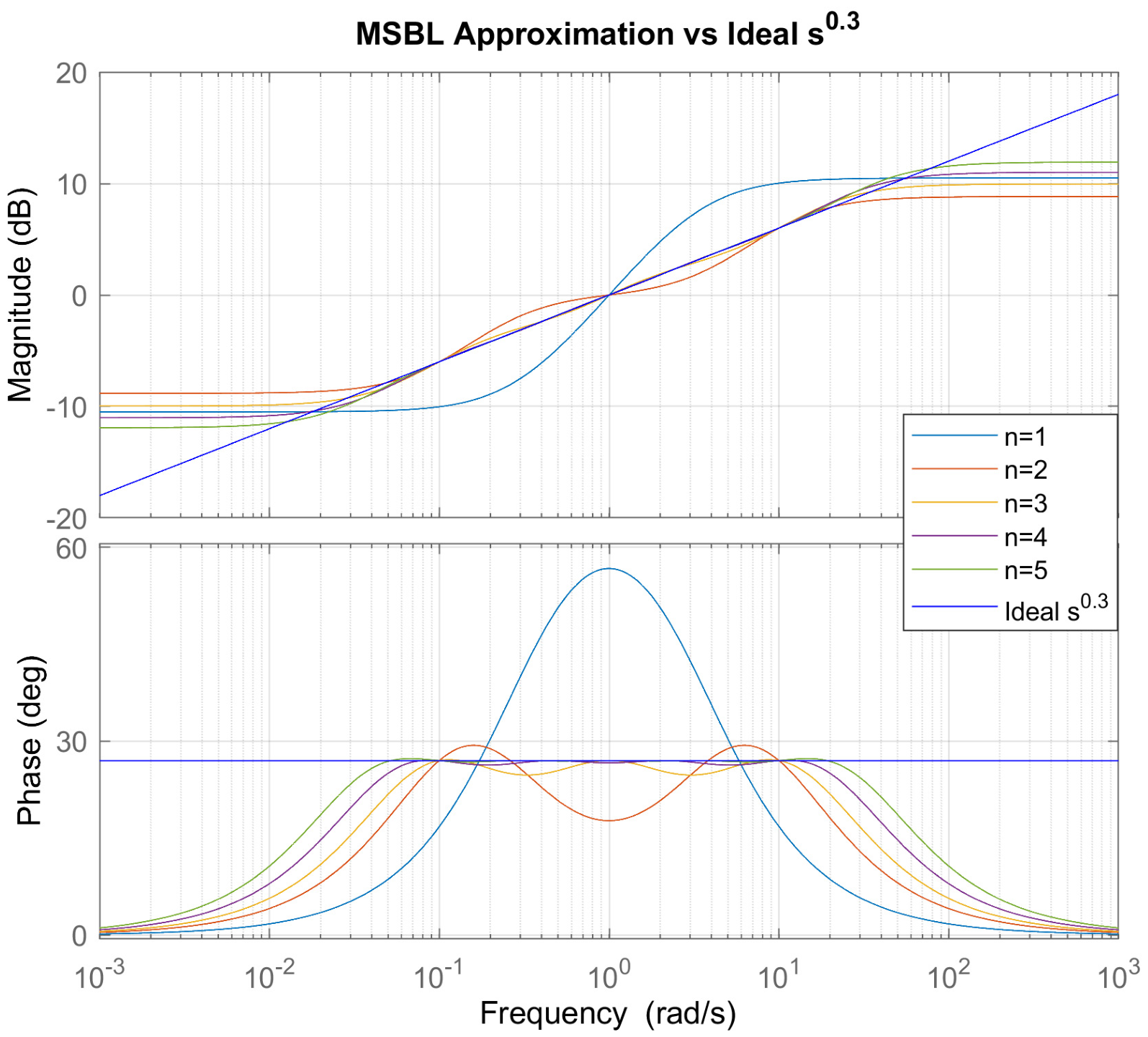
Figure 6 illustrates the Bode magnitude and phase responses of the reference fractional-order operator s0.3, together with its Modified Stability Boundary Locus (M-SBL)-based rational approximations for approximation orders ranging from n = 1 to n = 5. The approximation frequency band was selected as 0.1 ≤ ω ≤ 10 rad/s.
Figure 6.
Bode response comparison for the fractional-order differentiator s0.3 with M-SBL-based integer-order approximations for approximation orders n = 1, 2, 3, 4, and 5 in the frequency band 0.1–10 rad/s.
It can be observed that low-order approximations (n = 1 and n = 2) provide only a coarse representation of the fractional-order behavior, exhibiting noticeable deviations in both magnitude slope and phase response. With increasing approximation order, the M-SBL models progressively improve the agreement with the reference fractional response. In particular, higher-order approximations (n ≥ 4) closely match the constant phase characteristic and the magnitude slope of the fractional-order operator within the selected frequency band.
The findings indicate that the M-SBL approach successfully represents the stability boundary characteristics of the fractional-order operator, while ensuring stability of the resulting rational models. The improvement in approximation accuracy with increasing order highlights the inherent trade-off between model complexity and fidelity. Nevertheless, even moderate approximation orders provide stable and physically realizable transfer functions suitable for frequency-domain and time-domain analyses.
2.6. Equal-Ripple Biquadratic Approximation
To obtain low-order realizations of fractional integrators and differentiators, a biquadratic rational approximation derived from the Continued Fraction Expansion (CFE) can be employed. For a fractional operator sα, 0 < α < 1, a second-order symmetric approximation is written as [25]
The numerator and denominator have a symmetric biquadratic structure. However, this structure alone does not guarantee stability. The stability of the approximation depends on the selected coefficients and the corresponding parameter conditions. Therefore, the stability condition given in (29) must be satisfied to ensure that all poles of the approximation lie in the left-half complex plane.
The coefficients are defined as
where β is a tuning parameter introduced to control the magnitude and phase errors. Unlike classical CFE, the parameter β is selected such that the maximum approximation errors are uniformly distributed over the frequency band, yielding an Equal-Ripple response.
To ensure stability of the approximation, β must satisfy [26]
The frequency-domain approximation error is expressed as follows:
The optimal value of β is chosen so that
which minimizes the worst-case deviation across the operating band.
To extend the effective frequency range, multiple frequency-scaled biquadratic sections are cascaded. The second-stage approximation is given by [27].
which explicitly expands to
Similarly, the third-stage approximation is obtained by cascading three frequency-shifted sections:
Each additional stage introduces a scaled copy of the base biquadratic block, thereby increasing the approximation order, while preserving the Equal-Ripple property. This construction significantly improves magnitude and phase matching over wider frequency intervals.
2.7. Exact-Phase Approximation
The Exact-Phase Biquadratic Approximation is a rational modeling technique for fractional Laplacian operators sα, 0 < α < 1, constructed to enforce zero phase error at a selected center frequency, typically normalized to ω = 1 rad/s. Unlike Equal-Ripple approximations, which distribute magnitude error uniformly, this method explicitly guarantees an exact phase contribution of απ/2 at the normalization frequency, thereby improving phase fidelity of the fractional operator [27].
The fractional operator is approximated by a symmetric biquadratic transfer function
To impose zero phase error at ω = 1, the middle coefficient is chosen as
This selection guarantees
thereby ensuring exact phase correspondence with the reference fractional operator at the center frequency.
The coefficients a0 and a2 are not uniquely defined, and are selected to balance the approximation bandwidth against the desired accuracy. A generalized parameterized formulation is given by [25]
where β1, β2 and v are real tuning parameters. These parameters introduce additional degrees of freedom, allowing adjustment of the gain slope and approximation bandwidth. The systematic optimization of these parameters is application-dependent, and remains an open design choice.
Because a single biquadratic stage provides accurate behavior only over a limited frequency interval, wider bandwidths are achieved through cascading frequency-scaled sections.
The double-stage realization is expressed as
while the triple-stage realization becomes
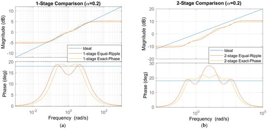
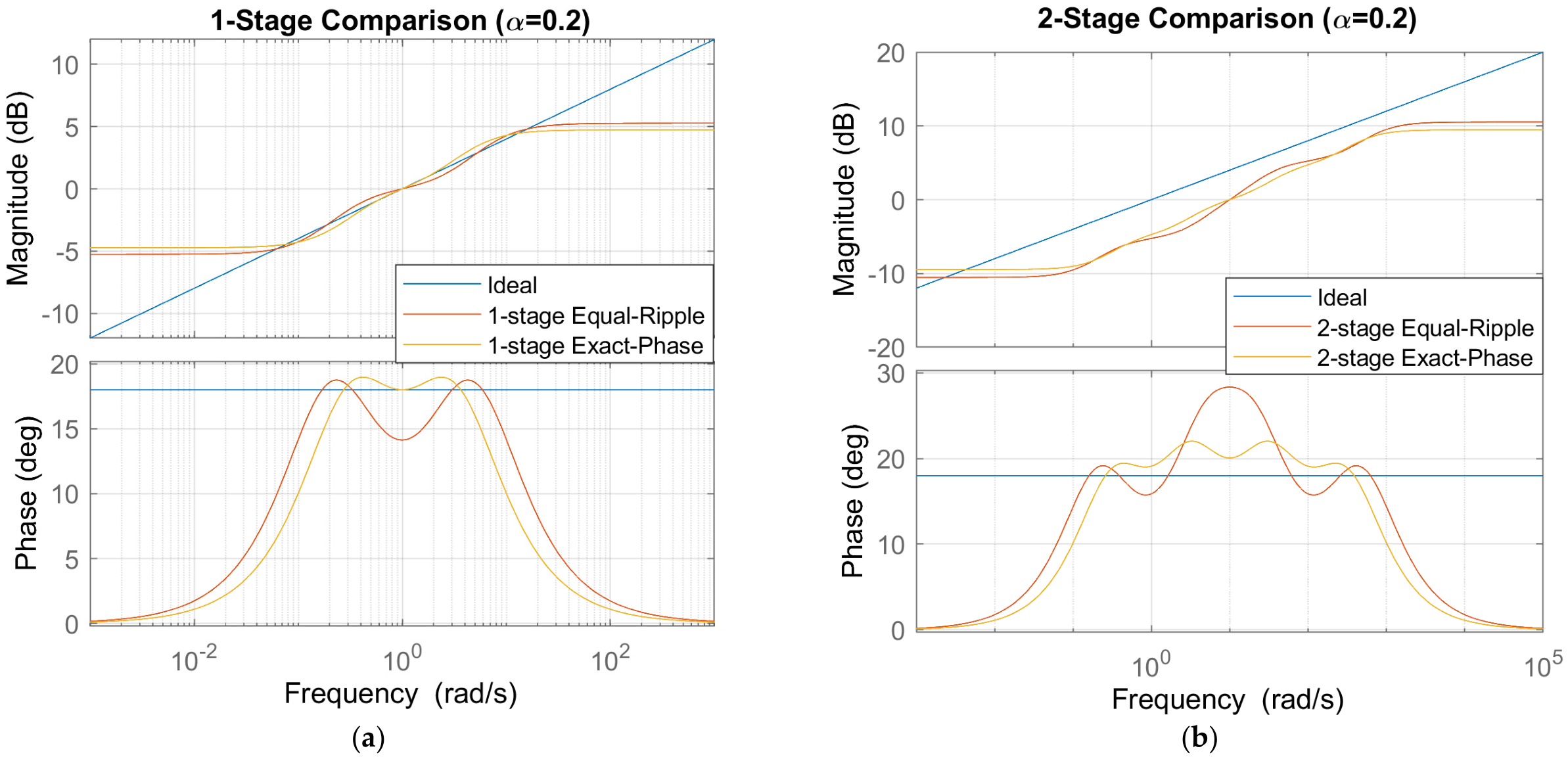
The comparative analysis across one- and two-stage realizations, as shown in Figure 7a,b, demonstrates that increasing the number of cascaded biquadratic sections significantly enhances the approximation accuracy of both Equal-Ripple and Exact-Phase methods. While single-stage implementations provide only localized matching around the design frequency, multi-stage architectures systematically extend the effective bandwidth and improve magnitude and phase conformity with the ideal fractional operator. The Equal-Ripple approach consistently achieves more uniform magnitude performance over wide frequency ranges by suppressing peak approximation errors, whereas the Exact-Phase method maintains superior phase alignment near the operating point. As the number of stages increases, both techniques exhibit substantial reductions in approximation error, confirming that cascading frequency-scaled sections offers a practical and scalable strategy for realizing fractional-order operators. The rational transfer functions obtained using the Equal-Ripple and Exact-Phase approaches are presented in Table 7 and Table 8, respectively. These results highlight an inherent trade-off between magnitude uniformity and phase accuracy, suggesting that Equal-Ripple approximations are preferable for broadband magnitude-sensitive applications, while Exact-phase approximations are more suitable for control-oriented designs, where phase fidelity is critical.
Figure 7.
(a) Bode plots showing magnitude and phase responses of the reference fractional operator s0.2 compared with the first-stage Equal-Ripple and Exact-Phase approximations, (b) Bode plots showing magnitude and phase responses of the reference fractional operator s0.2 compared with the second-stage Equal-Ripple and Exact-Phase approximations.
Table 7.
Transfer Functions of Equal-Ripple Approximation for s0.2 at different stages.
Table 8.
Transfer Functions of Exact-Phase Approximation for s0.2 at different stage.
3. Test Systems and Simulation Framework
This section defines the test systems and simulation framework used to systematically evaluate the accuracy of the investigated rational approximation methods. Three fractional-order models with different levels of complexity are considered: a fundamental fractional-order operator, a higher-order fractional-order transfer function, and a fractional-order controller. The common simulation conditions and approximation settings are then specified, to provide a consistent basis for comparison. Finally, the frequency-domain and time-domain metrics used to quantify approximation accuracy are defined.
3.1. Selection of Fractional-Order Test Systems
To evaluate the rational approximation methods at different levels of complexity, three fractional-order test systems were selected. The test cases include a fundamental fractional-order operator, a higher-order fractional-order transfer function, and a fractional-order controller. These systems provide progressively more complex examples for investigating the applicability of the approximation methods.
3.1.1. Fractional Order Operator sα
The first test case considers the fractional-order operator
where α denotes the fractional order. In this study, the operator G(s) = s0.5 was selected as a representative example of a half-order differentiator. This operator represents a fundamental fractional element, and provides a simple benchmark before considering more complex fractional-order systems. Different values of α change the magnitude slope and phase angle of the ideal operator, potentially affecting the accuracy of its rational approximations. Therefore, the results for α = 0.5 provide a reference for comparing the approximation methods, but do not necessarily establish the same performance ranking for all fractional orders.
3.1.2. Higher-Order Fractional-Order Transfer Function
The second test case is a higher-order fractional-order transfer function given by [28]
The model contains two fractional-order terms, s1.31 and s0.97, and therefore represents a more complex fractional-order dynamic system than the single fractional operator.
This system was selected to examine the approximation methods in a higher-order fractional-order transfer-function structure.
3.1.3. Fractional-Order Controller
The third test case is the fractional-order controller
The controller contains proportional, fractional integral, and fractional derivative terms. It can be represented in the general PIλDμ form as
where Kp = 2, Ki = 1.5, and Kd = 0.8 with fractional order λ = 0.7 and μ = 0.5.
This controller was selected as a control-oriented test case containing both fractional integration and differentiation.
3.2. Simulation Setting
All simulations were performed using MATLAB R2020b (Release 9.9, Update 8). The fractional-order models were implemented using the FOMCON toolbox (version 1.50.4), while the rational approximations were constructed using the corresponding approximation algorithms [29,30]. The simulation framework was established to provide a consistent basis for evaluating the frequency- and time-domain accuracy of the investigated approximation methods.
3.2.1. Approximation Order and Frequency Range
A nominal approximation order of 4 was selected for the methods, using an order parameter, while the Equal-Ripple and Exact-Phase methods were configured using their respective method-specific parameters.
The approximation frequency range was set to ([ωb,ωh] = [0.001, 1000]) rad/s for all three test systems. The frequency responses were evaluated using 500 logarithmically spaced points over the wider interval, from 10−4 to 104 rad/s.
It should be noted that the approximation-order parameter is method-dependent, and does not necessarily correspond to the same rational model degree or computational complexity across all methods. Therefore, these settings do not represent equal-order or equal-complexity conditions. The comparison primarily focuses on approximation accuracy under consistent test-system and frequency-range conditions, rather than on computational efficiency.
3.2.2. Time-Domain Simulation Setting
For the time-domain evaluation, unit-step responses were obtained for the original fractional-order models and their corresponding rational approximations. The original fractional-order responses, generated using the FOTF Viewer of the FOMCON toolbox, were considered as reference responses. The rational approximation models were simulated in MATLAB, using the lsim function, with the same unit-step input and corresponding time vector as the reference response.
The approximation error was calculated from the difference between the reference and rational-model responses. The same simulation conditions were maintained for all approximation methods within each test case, to ensure a consistent evaluation of their time-domain performance. The resulting responses were subsequently compared using the time-domain error metrics described in Section 3.3.
3.3. Performance Evaluation Metrics
The approximation accuracy was evaluated in both the frequency and time domains by comparing the rational approximations with the original fractional-order models.
3.3.1. Frequency-Domain Evaluation
For the frequency-domain analysis, the root-mean-square error (RMSE) was calculated separately for the magnitude and phase responses.
The magnitude responses were converted into decibels, using
The magnitude RMSE is calculated as
The phase RMSE is calculated as
where M represents the total number of frequency points. Magapp and Magref denote the approximate and reference magnitude responses, respectively, while Phaseapp and Phaseref represent their corresponding phase responses in degrees. Both phase responses are unwrapped before calculating the phase error.
3.3.2. Time-Domain Evaluation
For the time-domain analysis, the step responses of the rational approximations were compared with the corresponding reference responses. The response error is defined as
where yref(t) and yapp(t) represents the reference and approximate responses, respectively.
The time-domain RMSE is calculated as
where L is the total number of time samples.
The integral absolute error (IAE) and integral squared error (ISE) were also used to evaluate the accumulated approximation error. They are calculated as
Both integrals are evaluated from the initial simulation time (t0) to the final simulation time (tf), using numerical trapezoidal integration.
The magnitude RMSE is expressed in decibels (dB), the phase RMSE in degrees (°), and the time-domain RMSE in the same unit as the system output. IAE is expressed in output units multiplied by seconds, while ISE is expressed in squared output units multiplied by seconds. Lower error values indicate better agreement between the rational approximation and the reference model.
4. Result and Discussion
The performance of the investigated rational approximation methods is evaluated using the three selected fractional-order test systems. The analysis covers the fundamental fractional-order operator, the higher-order fractional-order transfer function, and the fractional-order controller. Both frequency- and time-domain results are considered, to assess how accurately the rational approximations reproduce the original fractional-order models.
4.1. Approximation of the Fundamental Fractional Operator
4.1.1. Frequency-Domain Comparison
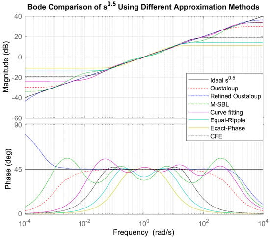
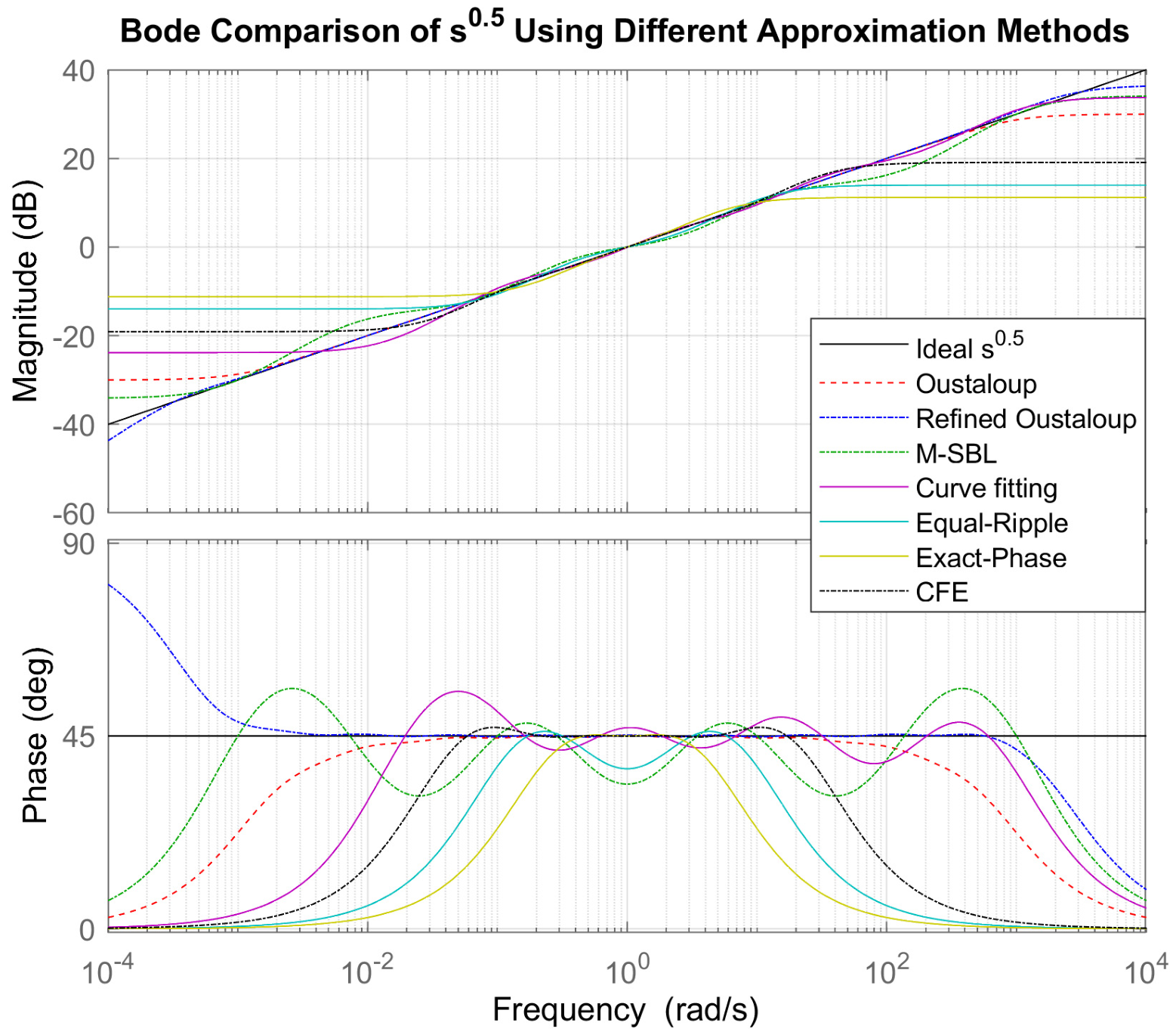
The frequency responses of the rational approximations of s0.5 are compared with the reference fractional-order operator over the considered frequency range. As shown in Figure 8, the reference response has a magnitude slope that remains at 10 dB per decade and a phase angle fixed at 45°. The rational approximations reproduce these characteristics to different degrees, with the largest deviations appearing at the lower and upper edges of the selected frequency band.
Figure 8.
Different rational approximations of the fractional operator s0.5 over the frequency range 10−3–103 rad/s.
Among the investigated methods, the Refined Oustaloup approximation follows the reference magnitude and phase responses most closely over the central frequency region. Classical Oustaloup and M-SBL also provide relatively close approximations, although larger deviations can be observed near the frequency boundaries. The remaining methods show more noticeable differences in either magnitude, phase, or both.
The quantitative results in Table 9 support these observations. The Refined Oustaloup method gives the lowest-magnitude and -phase RMSE, with values of 0.7533 dB and 11.107°, respectively. M-SBL and Classical Oustaloup follow, with magnitude RMSE values of 2.2364 dB and 2.9952 dB, and phase RMSE values of 14.748° and 18.819°, respectively. Curve Fitting gives intermediate accuracy, while the Equal-Ripple, Exact-Phase and CFE approximations show larger deviations from the reference fractional response.
Table 9.
Frequency-domain approximation errors for s0.5.
Overall, the frequency-domain comparison shows that the approximation methods differ considerably in their ability to preserve the characteristic magnitude and phase behavior of the fractional operator.
4.1.2. Effect of Approximation Order
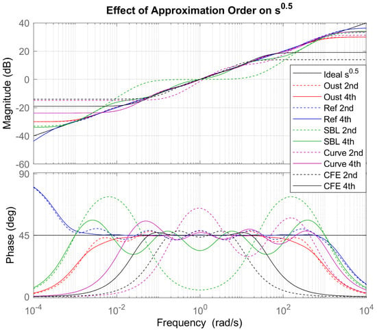
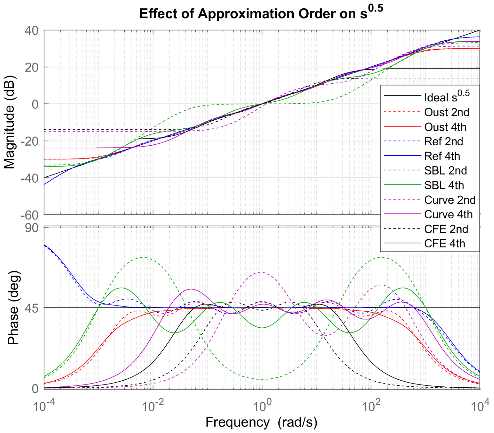
The effect of approximation order on the representation of s0.5 is shown in Figure 9, where second- and fourth-order approximations are compared for the investigated methods. Increasing the approximation order generally provides additional flexibility for reproducing the reference fractional-order characteristics, particularly over the central part of the frequency range.
Figure 9.
Effect of approximation order on the Bode magnitude and phase responses of s0.5 using second- and fourth-order rational approximations.
The effect is not identical for all methods. For some approximations, the fourth-order representation produces a visibly closer magnitude slope and phase response, whereas the improvement is more limited for others. The most noticeable differences between the two orders typically occur at the edges of the selected approximation band, where the rational models deviate more strongly from the reference fractional response.
The comparison also illustrates the balance between approximation precision and the complexity of the resulting model. A higher approximation order introduces additional poles and zeros, and therefore increases the complexity of the resulting rational model. Consequently, increasing the order can improve the frequency-domain representation, but the benefit should be considered together with the resulting model complexity.
4.2. Approximation of the Higher-Order Fractional Order Transfer Function
4.2.1. Bode Comparison
The frequency-domain responses of the higher-order fractional-order transfer function and its rational approximations are shown in Figure 10. Compared with the fundamental s0.5 operator, the higher-order model produces a more demanding approximation problem because the response is determined by the combined effect of the fractional terms s1.31 and s0.97. The approximations show different levels of agreement with the original fractional-order model, particularly in the phase response and toward the boundaries of the frequency range.
Figure 10.
Bode magnitude and phase plots comparing the original fractional-order system with various rational approximation methods, illustrating the approximation accuracy across the frequency range 10−3–103 rad/s.
The Refined Oustaloup approximation follows the reference magnitude and phase responses most closely over the considered frequency range. M-SBL also maintains relatively good agreement, although its deviations become more noticeable in parts of the frequency range. Classical Oustaloup shows larger deviations, while Curve Fitting, CFE, Equal-Ripple, and Exact-Phase exhibit progressively larger differences from the reference response, particularly in the phase characteristics.
4.2.2. Magnitude and Phase Error
The quantitative frequency-domain errors are summarized in Table 10. The Refined Oustaloup method gives the lowest magnitude and phase RMSE, with values of 0.4367 dB and 5.4685°, respectively. M-SBL gives the next lowest errors, with 1.2637 dB magnitude RMSE and 7.423° phase RMSE. Classical Oustaloup results in 3.691 dB and 17.194°, while Curve Fitting gives 4.3488 dB and 19.703°.
Table 10.
Frequency-domain approximation errors for the higher-order fractional-order transfer function.
The remaining methods show substantially larger deviations. The magnitude RMSE increases to 5.8266 dB for CFE, 9.3349 dB for Equal-Ripple, and 12.117 dB for Exact-Phase. A similar trend is observed for the phase error, with RMSE values of 21.557°, 28.864°, and 34.412°, respectively. These results indicate that the differences observed in the Bode plots are also reflected in the quantitative frequency-domain evaluation.
4.2.3. Step-Response Comparison
The corresponding time-domain responses are presented in Figure 11. The black curve represents the reference fractional-order response, while the remaining curves represent the rational approximations. The step response provides an additional perspective on how well the approximated transfer functions preserve the dynamic behavior of the original model.
Figure 11.
Step-response comparison of the fractional plant (FOMCON reference) and its rational approximations, including a zoomed view highlighting small response deviations.
The Refined Oustaloup response remains very close to the reference throughout the simulation interval. M-SBL also follows the reference response relatively well, although a larger deviation develops with increasing time. In contrast, the other approximations show more pronounced differences in the response magnitude. In particular, Equal-Ripple and Exact-Phase remain substantially below the reference response, while CFE, Curve Fitting, and Classical Oustaloup also exhibit considerable deviations.
4.2.4. Time-Domain Error Analysis
The quantitative step-response errors are summarized in Table 11. The Refined Oustaloup approximation again provides the lowest errors across all three metrics, with an RMSE of 0.014124, an IAE of 117.91, and an ISE of 1.9948. M-SBL follows, with an RMSE of 0.032257, an IAE of 270.81, and an ISE of 10.405.
Table 11.
Time-domain approximation errors for the higher-order fractional-order transfer function.
The remaining methods produce substantially larger time-domain errors. Classical Oustaloup gives an RMSE of 0.26258, while Curve Fitting and CFE give 0.28587 and 0.28307, respectively. Equal-Ripple and Exact-Phase produce the largest deviations, with RMSE values of 0.33234 and 0.34749. The same general trend is observed for IAE and ISE, where the largest accumulated errors are obtained for Equal-Ripple and Exact-Phase.
4.2.5. Discussion
The frequency- and time-domain results show a consistent trend for the higher-order fractional-order transfer function. The Refined Oustaloup method provides the closest approximation to the reference model across all evaluated metrics, while M-SBL also maintains relatively small deviations. The agreement between the frequency-domain and time-domain results is particularly important because it indicates that the smaller frequency-response errors of these methods translate into closer reproduction of the system’s dynamic response. Conversely, the larger frequency-domain deviations observed for Equal-Ripple, Exact-Phase, CFE, and the other approximations are accompanied by larger step-response errors.
4.3. Approximation of the Fractional-Order Controller
4.3.1. Bode Comparison
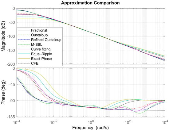
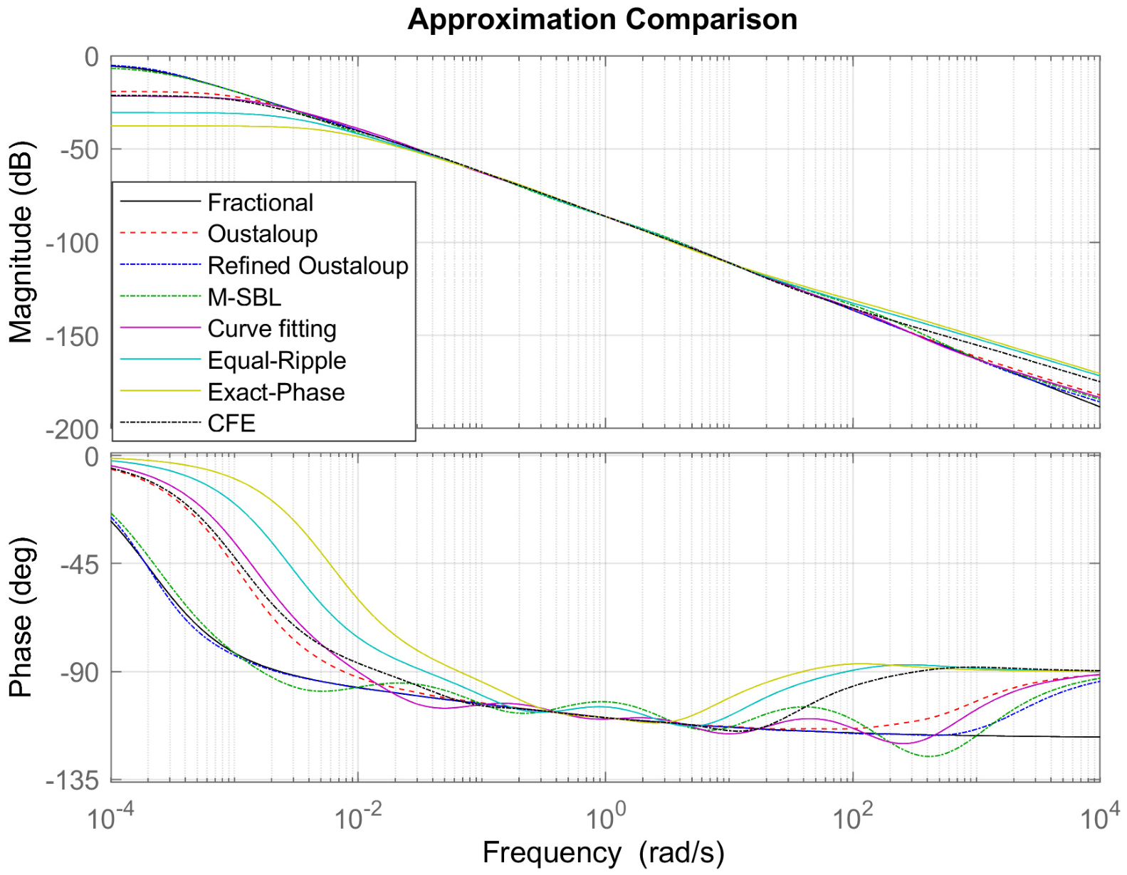
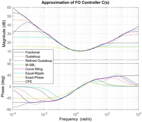
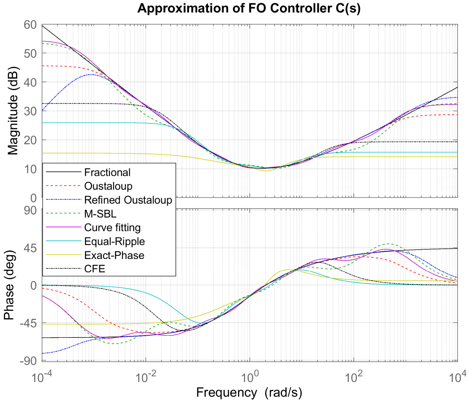
The frequency-domain responses of the fractional-order controller and its rational approximations are shown in Figure 12. The approximations reproduce the general shape of the reference controller response in the central frequency region, but noticeable differences appear toward the lower- and upper-frequency ranges. The magnitude and phase responses show that the approximation accuracy varies considerably among the investigated methods.
Figure 12.
Bode plots showing magnitude and phase responses of the fractional-order controller and its rational approximations over the frequency range 10−3–103 rad/s.
The Refined Oustaloup approximation follows the reference phase response relatively closely, particularly around the central frequency region, although its magnitude response shows noticeable deviations at the frequency boundaries. Curve Fitting provides a close magnitude response over a large part of the frequency range, while M-SBL also maintains relatively good agreement with the reference. In contrast, Equal-Ripple, Exact-Phase, and fourth-order CFE exhibit larger deviations in both magnitude and phase.
4.3.2. Magnitude and Phase Error
The quantitative frequency-domain results are summarized in Table 12. Curve Fitting gives the lowest magnitude RMSE of 1.3169 dB, followed by M-SBL with 1.9111 dB. Classical Oustaloup gives 3.5493 dB, while the Refined Oustaloup approximation gives a higher magnitude RMSE, of 5.9308 dB. The remaining methods show substantially larger magnitude deviations, particularly Exact-Phase, with 17.964 dB.
Table 12.
Frequency-domain approximation errors for the fractional-order controller.
For the phase response, however, the Refined Oustaloup method gives the lowest RMSE, at 9.0074°. M-SBL and Curve Fitting provide similar phase errors, of 15.327° and 15.299°, respectively. Classical Oustaloup results in 22.567°, while Equal-Ripple and fourth-order CFE show considerably larger phase errors. These results indicate that the frequency-domain performance depends on the response characteristic being considered: Curve Fitting provides the closest magnitude representation, whereas Refined Oustaloup provides the closest phase representation.
4.3.3. Step-Response Comparison
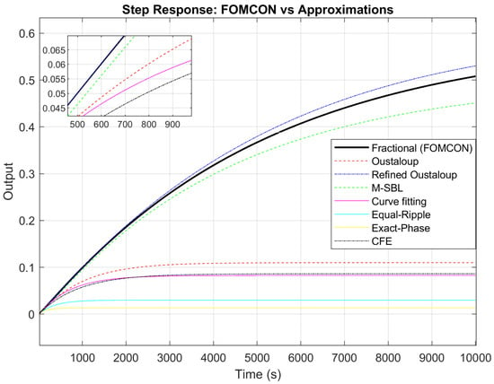
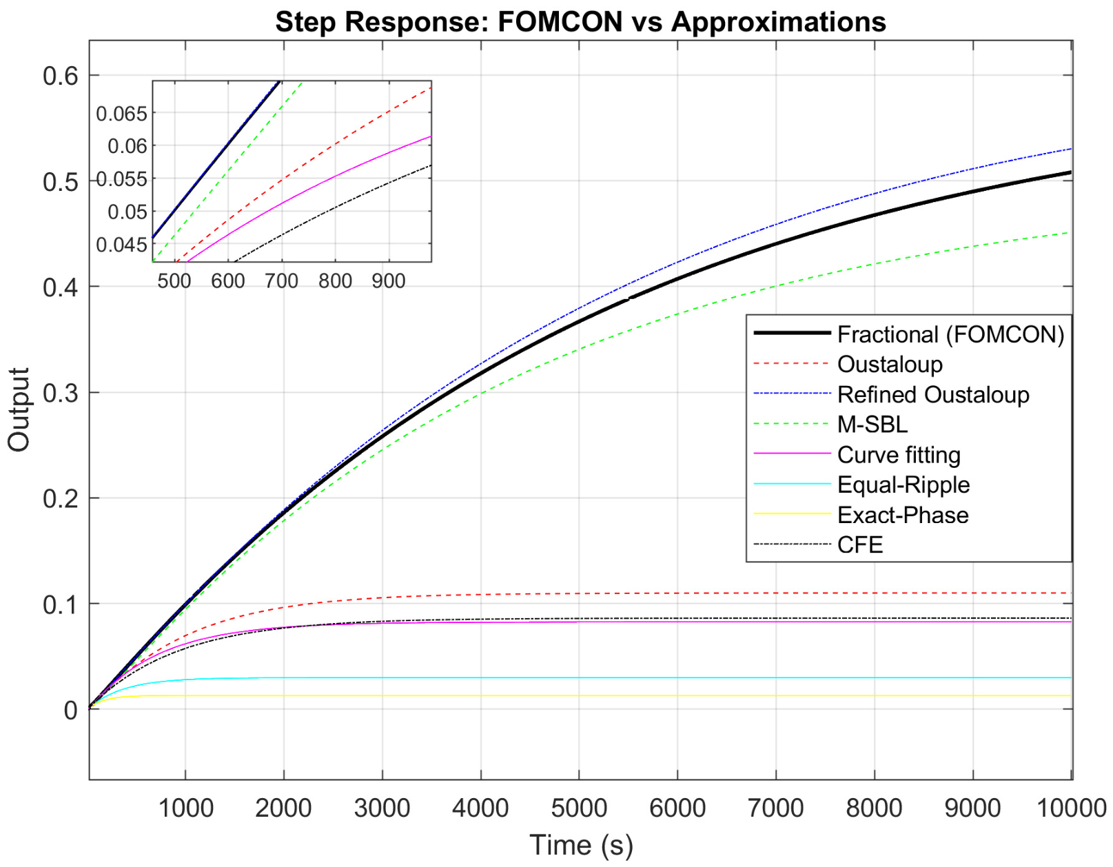
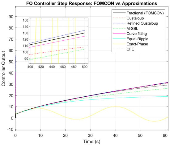
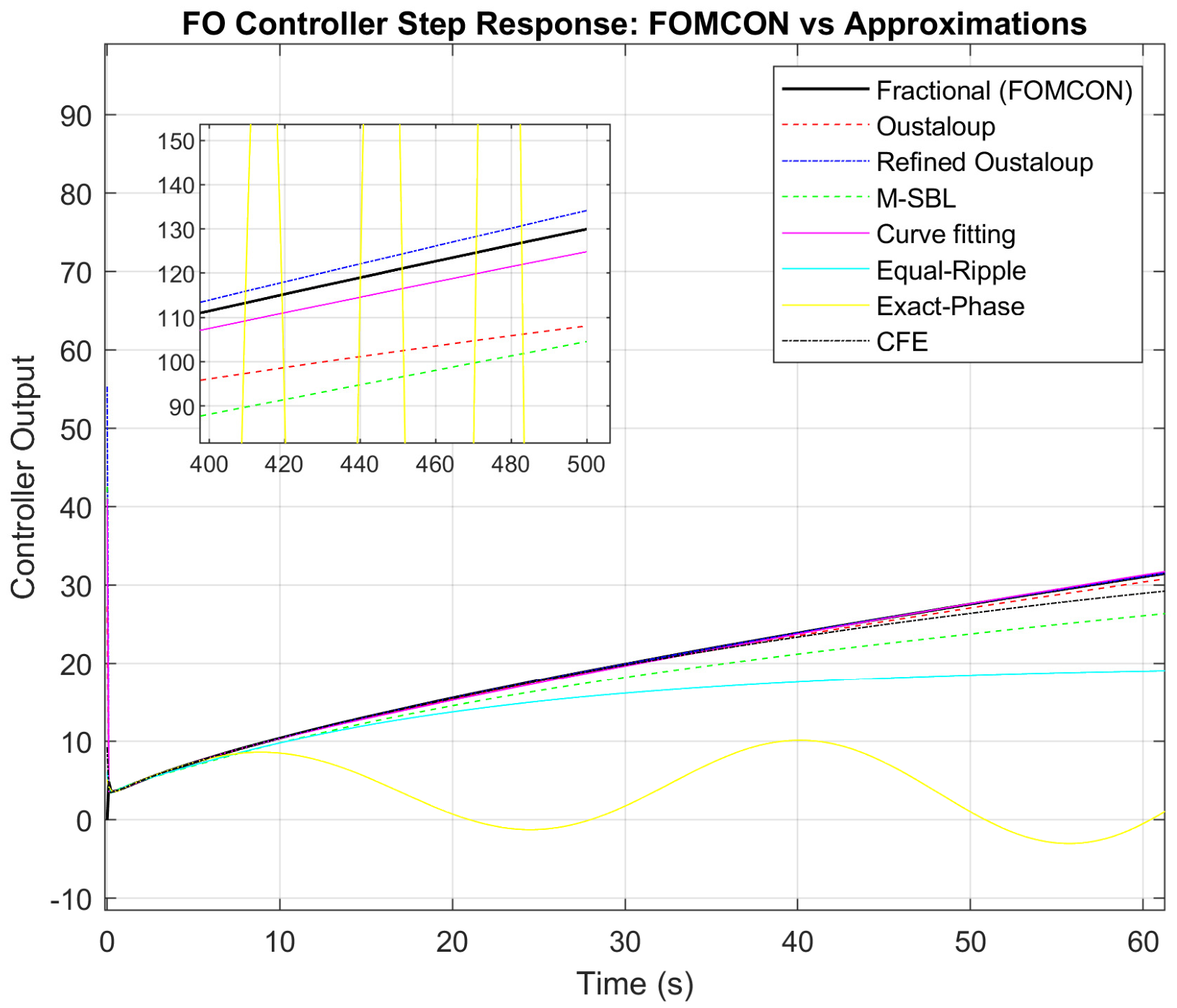
The time-domain responses of the fractional-order controller and its rational approximations are presented in Figure 13. The differences between the approximations become more apparent in the time domain than in the central region of the Bode plot. The Refined Oustaloup response remains closest to the reference response throughout the simulation interval. Curve Fitting also follows the reference relatively well, whereas classical Oustaloup shows a larger deviation.
Figure 13.
Step-response comparison of the FO-Controller (FOMCON reference) and its rational approximations, including a zoomed view highlighting transient deviations.
M-SBL exhibits a more noticeable deviation from the reference response, despite its relatively small frequency-domain errors. The Equal-Ripple and Exact-Phase approximations show substantially different dynamic behavior, with the Exact-Phase response exhibiting particularly large deviations. The fourth-order CFE approximation also departs considerably from the reference response.
4.3.4. Time-Domain Error Analysis
The quantitative time-domain results are given in Table 13. The Refined Oustaloup approximation produces the lowest error for all three measures, with an RMSE of 1.9275, an IAE of 633.43, and an ISE of 1704. Curve Fitting provides the next closest time-domain response, with an RMSE of 2.6549, an IAE of 978.32, and an ISE of 3439.5.
Table 13.
Time-domain approximation errors for the fractional-order controller.
The remaining methods result in substantially larger errors. Classical Oustaloup gives an RMSE of 10.675, while M-SBL gives 18.054, despite its relatively low frequency-domain errors. The CFE approximation produces an RMSE of 48.135. The largest deviations are obtained for Equal-Ripple and Exact-Phase, with RMSE values of 66.758 and 133.38, respectively. The IAE and ISE values show the same general trend, confirming the large accumulated deviations of these approximations over the simulation interval.
4.3.5. Discussion
The controller results highlight an important difference between frequency-domain and time-domain evaluation. While Curve Fitting provides the lowest magnitude RMSE and Refined Oustaloup provides the lowest phase RMSE, the Refined Oustaloup approximation gives the closest overall time-domain response. This indicates that good agreement in one frequency-domain characteristic does not necessarily translate directly into the smallest step-response error.
The results also show that the performance differences become more pronounced when the fractional approximation is incorporated into a controller model. In particular, the large time-domain errors obtained with Equal-Ripple, Exact-Phase, and CFE are consistent with their larger deviations in the frequency-domain responses. Overall, the controller case demonstrates the importance of evaluating rational approximations using both frequency- and time-domain measures, rather than relying on a single error criterion.
5. Conclusions
This study compared seven rational approximation methods using three fractional-order test systems: the fundamental operator, a higher-order fractional transfer function and a controller with fractional-order dynamics. The methods were evaluated using both frequency- and time-domain metrics.
The findings indicate that no individual method delivers the best performance in every case. Refined Oustaloup generally provided the closest approximation for the fundamental operator and higher-order transfer function, while for the fractional-order controller, Curve Fitting achieved the lowest-magnitude RMSE and Refined Oustaloup provided the lowest phase and time-domain errors. The results, therefore, show that approximation performance depends on both the system and the evaluation criterion.
The comparison also highlights the importance of evaluating rational approximations in both frequency and time domains. Good frequency-domain agreement does not always correspond to the smallest time-domain error, making the combined evaluation useful for assessing the overall fidelity of fractional-order approximations.
Future work will consider additional fractional-order systems, higher approximation orders, and computational complexity. Further investigation of closed-loop control, real-time implementation, and experimental validation will also be considered, to assess the practical applicability of the approximation methods.
Author Contributions
Conceptualization, M.A.S. and R.M.; methodology, M.A.S. and R.M.; software, M.A.S.; validation, M.A.S.; formal analysis, M.A.S.; investigation, M.A.S.; writing—original draft preparation, M.A.S.; writing—review and editing, A.A.W., I.S., M.T.R. and R.M.; visualization, M.A.S.; supervision, R.M. All authors have read and agreed to the published version of the manuscript.
Funding
This work was supported by the Internal Grant Agency of Tomas Bata University in Zlín, under the project number IGA/CebiaTech/2024/001.
Data Availability Statement
The data supporting the findings of this study are available from the corresponding author upon reasonable request. The results are based on simulation and numerical analysis.
Acknowledgments
The authors acknowledge the support of Tomas Bata University in Zlín for providing the research environment and computational resources.
Conflicts of Interest
The authors declare no conflicts of interest.
References
- Ata, E. Laplace Transform-Based Analytical Solutions of Generalized Caputo-Type Fractional-Order Dynamical Systems Incorporating Mittag-Leffler Functions. Comput. Sci. Math. Forum 2026, 14, 5. [Google Scholar] [CrossRef] [Scilit]
- Krajewski, W.; Viaro, U. On the Rational Approximation of Fractional Order Systems. In Proceedings of the 2011 16th International Conference on Methods & Models in Automation & Robotics, Miedzyzdroje, Poland, 22–25 August 2011; IEEE: Piscataway, NJ, USA, 2011; pp. 132–136. [Google Scholar]
- Toledo-Hernandez, R.; Rico-Ramirez, V.; Iglesias-Silva, G.A.; Diwekar, U.M. A Fractional Calculus Approach to the Dynamic Optimization of Biological Reactive Systems. Part I: Fractional Models for Biological Reactions. Chem. Eng. Sci. 2014, 117, 217–228. [Google Scholar] [CrossRef] [Scilit]
- Deniz, F.N.; Alagoz, B.B.; Tan, N.; Koseoglu, M. Revisiting Four Approximation Methods for Fractional Order Transfer Function Implementations: Stability Preservation, Time and Frequency Response Matching Analyses. Annu. Rev. Control 2020, 49, 239–257. [Google Scholar] [CrossRef] [Scilit]
- Mishra, T.; Singh, K.K.; Rao, N.; Nasiruzzaman, M. Riemann–Liouville Fractional Integral Form of Modified Baskakov-Type Operators: Approximation Properties and Statistical Convergence. Mathematics 2026, 14, 1028. [Google Scholar] [CrossRef] [Scilit]
- Özger, F.; Aslan, R. Riemann-Liouville Type Fractional Generalized -Bernstein-Kantorovich Operators. In Approximation Theory and Special Functions; Duman, O., Erkus-Duman, E., Eds.; Springer Proceedings in Mathematics & Statistics; Springer Nature: Cham, Switzerland, 2026; Volume 503, pp. 183–204. [Google Scholar]
- Atherton, D.P.; Tan, N.; Yüce, A. Methods for Computing the Time Response of Fractional-order Systems. IET Control Theory Appl. 2015, 9, 817–830. [Google Scholar] [CrossRef] [Scilit]
- Iqbal, A.; Shekh, R.R. A Comprehensive Study on Different Approximation Methods of Fractional Order System. Int. Res. J. Eng. Technol. (IRJET) 2016, 3, 1848–1853. [Google Scholar]
- Tavazoei, M.S.; Haeri, M. Rational Approximations in the Simulation and Implementation of Fractional-Order Dynamics: A Descriptor System Approach. Automatica 2010, 46, 94–100. [Google Scholar] [CrossRef] [Scilit]
- Wendimu, A.A.; Matušů, R.; Shaikh, I.; Wolde, M.K.; Roba, M.T.; Yareshe, F.T. A Unified Comparative Framework for Fractional-Order Operator Approximation with Pareto-Based Analysis. Fractal Fract. 2026, 10, 321. [Google Scholar] [CrossRef] [Scilit]
- Krajewski, W.; Viaro, U. A Method for the Integer-Order Approximation of Fractional-Order Systems. J. Frankl. Inst. 2014, 351, 555–564. [Google Scholar] [CrossRef] [Scilit]
- Mahata, S.; Kar, R.; Mandal, D. Optimal Approximation of Fractional-order Systems with Model Validation Using CFOA. IET Signal Process. 2019, 13, 787–797. [Google Scholar] [CrossRef] [Scilit]
- Oustaloup, A.; Levron, F.; Mathieu, B.; Nanot, F.M. Frequency-Band Complex Noninteger Differentiator: Characterization and Synthesis. IEEE Trans. Circuits Syst. I 2000, 47, 25–39. [Google Scholar] [CrossRef] [Scilit]
- Vinagre, B.M.; Podlubny, I.; Hernandez, A.; Feliu, V. Some Approximations of Fractional Order Operators Used in Control Theory and Applications. Fract. Calc. Appl. Anal. 2000, 3, 231–248. [Google Scholar]
- Merrikh-Bayat, F. Rules for Selecting the Parameters of Oustaloup Recursive Approximation for the Simulation of Linear Feedback Systems Containing PIλDμ Controller. Commun. Nonlinear Sci. Numer. Simul. 2012, 17, 1852–1861. [Google Scholar] [CrossRef] [Scilit]
- Wiora, J.; Wiora, A. Influence of Methods Approximating Fractional-Order Differentiation on the Output Signal Illustrated by Three Variants of Oustaloup Filter. Symmetry 2020, 12, 1898. [Google Scholar] [CrossRef] [Scilit]
- Marciniak, K.; Saleem, F.; Wiora, J. Influence of Models Approximating the Fractional-Order Differential Equations on the Calculation Accuracy. Commun. Nonlinear Sci. Numer. Simul. 2024, 131, 107807. [Google Scholar] [CrossRef] [Scilit]
- Xue, D.; Zhao, C.; Chen, Y. A Modified Approximation Method of Fractional Order System. In Proceedings of the 2006 International Conference on Mechatronics and Automation, Luoyang, China, 25–28 June 2006; IEEE: Piscataway, NJ, USA, 2006; pp. 1043–1048. [Google Scholar]
- Lampasiak, M.; Jagodziński, J. Analysis of Methods for Approximating Fractional Order Systems Based on Zero and Pole Values. In Proceedings of the 2025 26th International Carpathian Control Conference (ICCC), Starý Smokovec, High Tatras, Slovakia, 19–21 May 2025; IEEE: Piscataway, NJ, USA, 2025; pp. 1–6. [Google Scholar]
- Krishna, B.T. Studies on Fractional Order Differentiators and Integrators: A Survey. Signal Process. 2011, 91, 386–426. [Google Scholar] [CrossRef] [Scilit]
- Bingi, K.; Ibrahim, R.; Karsiti, M.N.; Hassam, S.M.; Harindran, V.R. Frequency Response Based Curve Fitting Approximation of Fractional–Order PID Controllers. Int. J. Appl. Math. Comput. Sci. 2019, 29, 311–326. [Google Scholar] [CrossRef] [Scilit]
- Sanathanan, C.; Koerner, J. Transfer Function Synthesis as a Ratio of Two Complex Polynomials. IEEE Trans. Autom. Control 1963, 8, 56–58. [Google Scholar] [CrossRef] [Scilit]
- Deniz, F.N.; Alagoz, B.B.; Tan, N.; Atherton, D.P. An Integer Order Approximation Method Based on Stability Boundary Locus for Fractional Order Derivative/Integrator Operators. ISA Trans. 2016, 62, 154–163. [Google Scholar] [CrossRef] [Scilit] [PubMed]
- Koseoglu, M.; Deniz, F.N.; Alagoz, B.B.; Alisoy, H. An Effective Analog Circuit Design of Approximate Fractional-Order Derivative Models of M-SBL Fitting Method. Eng. Sci. Technol. Int. J. 2022, 33, 101069. [Google Scholar] [CrossRef] [Scilit]
- El-Khazali, R. On the Biquadratic Approximation of Fractional-Order Laplacian Operators. Analog. Integr. Circuits Signal Process. 2015, 82, 503–517. [Google Scholar] [CrossRef] [Scilit]
- Freeborn, T.J.; Maundy, B.; Elwakil, A. Second Order Approximation of the Fractional Laplacian Operator for Equal-Ripple Response. In Proceedings of the 2010 53rd IEEE International Midwest Symposium on Circuits and Systems, Seattle, WA, USA, 1–4 August 2010; IEEE: Piscataway, NJ, USA, 2010; pp. 1173–1176. [Google Scholar]
- El-Khazali, R.; Tawalbeh, N. Realization of Fractional-Order Capacitors and Inductors. In Proceedings of the 5th Workshop on Fractional Differentiation and its Applications, Nanjing, China, 14–17 May 2012. [Google Scholar]
- Zhao, C.; Xue, D.; Chen, Y.Q. A Fractional Order PID Tuning Algorithm for a Class of Fractional Order Plants. In Proceedings of the IEEE International Conference Mechatronics and Automation, 2005, Niagara Falls, ON, Canada, 29 July–1 August 2005; IEEE: Piscataway, NJ, USA, 2005; pp. 216–221. [Google Scholar]
- Tepljakov, A.; Petlenkov, E.; Belikov, J. FOMCON: A MATLAB Toolbox for Fractional-Order System Identification and Control. Int. J. Microelectron. Comput. Sci. 2011, 2, 51–62. [Google Scholar]
- Li, Z.; Liu, L.; Dehghan, S.; Chen, Y.; Xue, D. A Review and Evaluation of Numerical Tools for Fractional Calculus and Fractional Order Controls. Int. J. Control 2017, 90, 1165–1181. [Google Scholar] [CrossRef] [Scilit]

Disclaimer/Publisher’s Note: The statements, opinions and data contained in all publications are solely those of the individual author(s) and contributor(s) and not of MDPI and/or the editor(s). MDPI and/or the editor(s) disclaim responsibility for any injury to people or property resulting from any ideas, methods, instructions or products referred to in the content. |
© 2026 by the authors. Licensee MDPI, Basel, Switzerland. This article is an open access article distributed under the terms and conditions of the Creative Commons Attribution (CC BY) license.