


Abstract
Backpropagation is less a single algorithm than a pipeline of choices: how the error signal is propagated, how the weight gradient is assembled, and how the update is applied. This paper revisits three consecutive steps and proposes small, mathematically transparent modifications that improve gradient scaling and conditioning without changing the represented function class. The resulting method, Conditioned Backpropagation(CBP), combines (i) a layerwise gradient-norm equalization that counters the geometric depth dependence of the backpropagated error; (ii) an activation-centering reparameterization that removes the dominant rank-one mean term from the per-layer curvature; and (iii) a damped diagonal preconditioner that is positive-definite by construction. The composite operator is a bounded positive-definite preconditioner, so the method inherits standard nonconvex, Polyak–Łojasiewicz, and stochastic convergence guarantees at the per-step cost of ordinary backpropagation. No prior method composes these three repairs into one operator with a joint boundedness and positive-definiteness guarantee. Two further results, both new, concern equalization. On a block-structured strongly convex model, and for the curvature-equalizing target that the implemented gradient-energy equalizer approximates up to a quantified heterogeneity factor, equalization makes the convergence rate depth-uniform; the bounded-clip version that is actually run stays depth-uniform up to a clip-determined depth and retains a constant-factor improvement beyond it. Controlled experiments, run over ten or more seeds with paired significance tests, confirm the mechanisms: Equalization compresses an order-of-magnitude per-layer gradient disparity, centering cuts the top curvature eigenvalue about threefold and yields the lowest training loss, and the configurations combining centering with the damped preconditioner, including the full method, converge fastest. The effects persist on MNIST and on CIFAR-10 with a small residual convolutional network, at a measured per-iteration overhead below about twice that of Adam. Generalization is comparable across methods, and no end-to-end depth-scaling advantage is claimed, keeping the contribution focused on optimization geometry.
1. Introduction
The backpropagation algorithm is so familiar that it is easy to forget how many distinct decisions it bundles together. At its core, it is a single application of the chain rule, but in practice, every implementation must also decide how the error signal is scaled as it traverses the layers, how that signal is combined with stored activations to form each weight gradient, and how the resulting gradient is turned into a parameter update. These are separate steps, and each of them shapes the geometry of the optimization problem that the learner actually faces. A large fraction of the engineering folklore of deep learning, including initialization rules, normalization layers, adaptive optimizers, gradient clipping, and learning-rate warmup, can be read as attempts to repair one or another of these steps so that the gradient signal is well scaled, stable, and informative [1,2,3].
Rather than proposing yet another monolithic optimizer, this paper isolates three consecutive steps of the backward pass and asks, for each, what minimal mathematical change improves the conditioning of the gradient while leaving the function computed by the network unchanged. The three steps and their corresponding modifications are as follows.
- M1.
- Error propagation. The backpropagated error has a second moment that grows or decays geometrically with depth; this is the classical vanishing/exploding-gradient phenomenon. Each layer’s gradient block is rescaled by a positive scalar estimated online so that all blocks carry a common second moment, a step referred to as layerwise gradient-norm equalization.
- M2.
- Gradient assembly. The weight gradient is an outer product of the error signal with the incoming activation. When the activation has a large mean (as rectified units do), this outer product inherits a dominant rank-one term that inflates the local curvature. Centering the incoming activation, an exact reparameterization, removes that rank-one term.
- M3.
- Update. A diagonal preconditioner built from a running estimate of the squared gradient is applied, regularized by a damping term that guarantees positive definiteness and bounded eigenvalues.
Individually, each ingredient is closely related to ideas that already exist in the literature: signal-propagation analyses of initialization [4,5], mean-removal and normalization schemes [1,6], and adaptive or curvature-aware optimizers [7,8]. The contribution here is to present them as three commuting operations on the backward pass, to give a unified and self-contained analysis showing that the combined operator is a bounded positive-definite preconditioner, and therefore a legitimate descent operator to which standard convergence guarantees apply, and to verify, in controlled experiments, the specific mechanisms the analysis predicts. The general convergence theorems themselves are not new: they are the textbook guarantees for preconditioned (stochastic) gradient descent with a bounded positive-definite preconditioner. The novelty lies in constructing such a preconditioner cheaply and provably from three interpretable steps and, for the equalization step, specifically, in a depth-uniform linear rate (Theorem 4) that the generic bounded-preconditioner results do not capture, since it depends on the block-diagonal structure M1 imposes, together with an analysis of the clipped equalizer that is actually run (Theorem 5), which turns the clip from an unanalyzed implementation detail into a sharp statement of the depth at which depth-uniformity is retained.
Stated explicitly, the novelty of this work is threefold. First, although each ingredient descends from a known family (depth-aware rescaling, mean removal, and diagonal adaptive scaling), no prior work composes the three as commuting operations on the backward pass and proves that the composite is a single bounded positive-definite preconditioner. Existing approaches modify the architecture (normalization), the objective (sharpness-aware training), or the update rule in isolation (adaptive optimizers), and not one supplies a joint guarantee for the assembled pipeline. Second, two of the theoretical results are new in themselves rather than inherited: the depth-uniform linear rate of Theorem 4, which converts a depth-dependent condition number into a depth-independent one on block-structured objectives, and the direct analysis of the clipped equalizer (Theorem 5), which to the best of the author’s knowledge is the first to treat the clipping that is actually run as an object of analysis and to derive from it a sharp crossover depth . Third, the experimental design is mechanism-level rather than leaderboard-level: Every theoretical claim is paired with a falsifiable measurement (the per-layer gradient disparity, the alignment of the activation mean with the top curvature eigenvector, and depth sweeps on the analyzed model problem), a methodological stance that large-scale benchmarking studies have argued is precisely what optimizer research lacks [3,9].
The specific contributions are as follows. First, Conditioned Backpropagation (CBP) is formalized as the composition of three modifications to consecutive backpropagation steps (Section 4), and it is shown to be implementable with extra work per iteration, where P is the number of parameters and the number of activations; for dense layers this is the same order as a single backward pass, although for layer types in which the activation count exceeds the parameter count, the activation term dominates. Second, the analysis (Section 5) establishes that (a) the composite update is a descent direction because the induced preconditioner is positive definite (Proposition 1); (b) equalization makes the expected per-layer gradient second moment independent of depth (Proposition 2); (c) centering reduces the conditioning of the per-layer curvature factor in the aligned-mean regime characteristic of rectified activations (Proposition 3); and (d) the resulting bounded preconditioned scheme inherits the standard nonconvex rate, linear convergence under a local Polyak–Łojasiewicz condition, and the stochastic rate (Theorems 1–3); and (e) going beyond these inherited guarantees, on a block-structured strongly convex objective and for the curvature-equalizing target, the equalization step converts the depth-dependent global condition number into a depth-uniform one, yielding a linear rate whose constant does not grow with depth (Theorem 4); the gradient-energy equalizer that is actually run matches that target only up to a heterogeneity factor , which the analysis quantifies and the experiments bound empirically, and the rate comes with an explicit exponential-in-depth separation from single-step-size descent on a model problem (Proposition 5); and (f) the bounded-clip equalizer that is actually implemented is analyzed directly: It stays depth-uniform up to a sharp clip-determined depth and retains a constant factor-R improvement of the condition number beyond it, where R is the clip range (Theorem 5, Corollary 1), a prediction that the measured disparity profile confirms. Third, each mechanism is corroborated with reproducible experiments run over ten or more seeds, with confidence intervals and paired significance tests (Section 6): a depth-24 network in which M1 compresses an order-of-magnitude per-layer gradient disparity toward parity; a measurement confirming that the mean is almost collinear with the top eigenvector () and that centering cuts the top curvature eigenvalue by a median factor of about three; a head-to-head comparison with a common-base factorial ablation, indicating that centering is the modification most responsible for the lowest training loss, that the damped preconditioner supplies the speed, and that the configurations combining the two converge fastest; a three-part depth study that confirms the depth-uniform rate of Theorem 4 exactly on the block-structured model problem (single-step-size descent grows geometrically with depth, while the equalized scheme stays constant), confirms in networks that the per-layer disparity driving the rate grows geometrically with depth, and adds a training-level study that delineates where the gradient-scale mechanism governs end-to-end training and identifies the complementary forward-signal component whose treatment is charted as future work; and a real-data evaluation on MNIST and CIFAR-10, the latter with a small residual convolutional network, in which the optimization effects persist and the measured wall-clock overhead stays modest. The scope of the evidence is stated as plainly as the findings: Generalization is comparable across methods, and the practical clipped form of M1 removes a bounded, clip-determined factor of that disparity at extreme depth, with the remaining mapped out as future work.
It is worth being explicit about what is not claimed. CBP is not a new state-of-the-art optimizer, and on shallow, easy problems, it is essentially tied with well-tuned baselines. No generalization improvement is claimed, and while the depth-uniform rate is confirmed on the model problem it analyzes, no end-to-end depth-scaling advantage in generalization is claimed for deep networks; the path toward one is charted in Section 8.2. The point of the paper is mathematical: to show that three inexpensive, individually justifiable edits to the backward pass compose into a single object with clean guarantees, and that the place they demonstrably help is optimization geometry, where centering drives the lowest training loss and the damped preconditioner the fastest convergence in the ablations reported below.
The remainder of the paper is organized as follows. Section 2 fixes notation and recalls the backpropagation pipeline, identifying the two pathologies (depth-dependent scale and poor curvature conditioning) that motivate the method. Section 3 situates the three modifications within the existing literature on optimizers, curvature-aware methods, normalization, and loss landscapes. Section 4 defines the three modifications precisely and assembles them into a single algorithm, illustrated by the schematic in Figure 1 and the pseudocode in Algorithm 1.
Section 5 is the analytical core: It shows that the induced preconditioner is bounded and positive definite, analyzes the two structural modifications in turn, records the convergence guarantees (including the depth-uniform rate for the equalization step and the rate of the clipped equalizer that is actually run, both of which go beyond the inherited bounds), and bounds the computational overhead. Section 6 reports a sequence of controlled experiments, each probing one part of the analysis: the two mechanism studies, the head-to-head comparison with its common-base factorial ablation and hyperparameter sensitivity analysis, a three-part depth study covering the model problem, the geometric premise in networks, and the predicted clip-determined crossover together with a training-level study of its end-to-end scope, and a real-data evaluation on MNIST and CIFAR-10 with measured wall-clock overhead. Section 7 discusses scope, the relationship to normalization and adaptive methods, the price of the boundedness guarantee (where the clipped-equalizer rate is interpreted), and limitations, and Section 8 concludes with a summary and directions for future work. A reader interested primarily in the method may proceed from Section 4 to the experiments; a reader interested in the guarantees will find the self-contained proofs in Section 5, with extended derivations in Appendix A, Appendix B and Appendix C.
2. Background and Notation
This section fixes the notation used throughout the paper and recalls the mechanics of the backward pass, so that the three modifications of Section 4 can be stated as precise operations on well-defined quantities. Section 2.1 lays out the forward and backward equations of a feedforward network and names the three steps modified later. The two pathologies the method is designed to address are then explained in terms of those equations (Section 2.2): the depth-dependent scale of the backpropagated error and the poor conditioning of the per-layer curvature. Throughout, vectors are columns, is the Euclidean norm, and is the Frobenius norm.
2.1. Feedforward Networks and Backpropagation
Consider a feedforward network with L layers. Writing for the input, the network computes, for ,
where , , and is an elementwise activation (with the identity at the output layer). Let denote a per-example loss and define the error signal . The backward pass computes
where ⊙ denotes the elementwise (Hadamard) product. Equation (3) is the error propagation step, and (4) is the gradient assembly step. For a softmax output with cross-entropy loss, the output error simplifies to the convenient form , where p is the predicted class distribution and y the one-hot label.
All trainable parameters are collected into a single vector , and denotes the empirical risk. The symbol denotes a per-layer gradient block and the full gradient. The number of activations (summed hidden widths) is denoted . Table 1 summarizes the notation used throughout.
Table 1.
Summary of notation.
2.2. Why the Three Steps Matter
Two recurring pathologies motivate the modifications introduced below, and both can be read directly off the equations of the backward pass. The first concerns the scale of the gradient signal as it crosses many layers; the second concerns the conditioning of the local geometry that each layer’s update must navigate. Each is described in turn, because each is tied to a specific step of the pipeline and therefore admits a targeted repair.
Depth-dependent scale. The recursion (3) multiplies the error by a weight matrix and an activation-derivative mask at every layer. Under the usual signal-propagation model, the second moment of therefore evolves multiplicatively with depth, so that early layers can receive gradients that are many orders of magnitude smaller (or larger) than late layers [4,5,10]. A single global learning rate then under-trains some layers and destabilizes others.
Poor curvature conditioning. Even when scales are controlled, the local geometry seen by each layer can be badly conditioned. The Gauss–Newton/Fisher curvature block for factorizes (in the Kronecker-factored approximation) into an output factor and an input factor [8]. When the activation has a large mean, as it does for rectified units, which are nonnegative and so have a mean far from zero, this input factor is dominated by a rank-one mean term, and the condition number of the optimization problem suffers [1,11]. Recent work has tied such conditioning to training instability at the edge of stability and to the gap between adaptive and non-adaptive methods on modern architectures [2,12,13].
Conditioned Backpropagation attacks these two pathologies at the three steps where they originate. Each modification is local to one step, requires no architectural change, and is cheap enough to run at every iteration, so the repairs can be applied together without changing the asymptotic cost of training. The next section places the modifications in the context of the methods they build on, and Section 4 then states them precisely.
3. Related Work
Each of the three modifications has antecedents in a distinct strand of the literature, and the contribution of this paper lies as much in combining and analyzing them jointly as in any single piece. Four threads are relevant: rules for turning gradients into updates, curvature-aware optimization, normalization and initialization, and the study of optimization landscapes. The relationship of each thread to a specific modification is made explicit where it arises.
A long line of work modifies how gradients become updates. Adaptive moment methods descending from Adam [14], including the decoupled weight-decay variant AdamW [15], and their refinements remain the default for many architectures [16,17,18], and recent symbolic-search and schedule-free methods continue to push the design space [19,20,21], while sharpness-aware objectives reshape what is minimized to favor flat minima [22]. Large-scale benchmarks caution that, once tuned, many optimizers perform comparably, which raises the bar for claims of universal superiority and motivates the present emphasis on mechanism rather than leaderboard position [3]. A complementary thread explains why adaptive methods help: through curvature heterogeneity across parameter blocks [13,23], through sign-descent-like behavior [24], and through heavy-tailed class imbalance in language data [25]. The diagonal preconditioner M3 is an Adam-style second-moment scaler; what differs here is that it is treated as one of three composable steps and analyzed as a damped, bounded positive-definite operator, with the standard caveat that the empirical Fisher diagonal it uses is only a coarse curvature surrogate [24].
Curvature is used explicitly by second-order and natural-gradient methods [7,8]. Full or Kronecker-factored curvature is expensive; M2 and M3 together can be seen as a cheap diagonal-plus-centering surrogate that captures two specific, analyzable effects of curvature (the rank-one mean term and per-coordinate scale) without forming any matrix.
Normalization layers and careful initialization reshape the forward pass so that the backward pass behaves well [1,4,6,26]. Mean-removal in particular is a known ingredient of batch and layer normalization; the present treatment isolates it as an exact reparameterization (M2) and supplies a direct conditioning argument, though it captures only the mean-removal component of normalization, not variance scaling or a learned affine map. Signal-propagation analyses of depth and of transformers [5,10,27,28] motivate the equalization step M1, which is an adaptive, data-driven relative of depth-aware residual scaling and of layer-wise adaptive learning-rate schemes; M1 is not claimed to be wholly novel, but rather to be a correctness-preserving, analyzable instance of that family. The closest members of that family are the layerwise trust-ratio methods LARS [29] and LAMB [30], which scale each layer’s update by the ratio of the parameter norm to the update norm and were designed to stabilize large-batch training. M1 differs in target and in guarantee; it equalizes the estimated gradient second moment across layers rather than tying the step to the parameter norm, and its clipped form is part of a composite operator with a joint boundedness and positive-definiteness proof, together with the depth-uniform rate of Section 5.5 that trust-ratio methods do not provide. Both methods are included as baselines in the revised experiments of Section 6.3. Width-aware parameterizations that make hyperparameters transferable across scale [31] pursue the related goal of taming scale through a fixed reparameterization rather than online estimation.
Closest in spirit to M1 is the literature on gradient scaling and stability: Gradient clipping accelerates training under relaxed smoothness [32], and adaptive gradient clipping enables normalizer-free training [6]. M1 differs in intent, in that rather than bounding the global gradient norm it equalizes norms across layers, addressing depth-dependent disparity rather than outliers in time.
Finally, the convergence analysis draws on the structure of modern optimization landscapes. Over-parameterized networks frequently satisfy a Polyak–Łojasiewicz condition on neighborhoods of the interpolation manifold [33], which is the structure the local linear-rate result exploits. Conditioning and the loss-Hessian spectrum also govern training instability [2,12,34], the scientific-computing setting of physics-informed networks [35,36,37], and the practicalities of training very deep transformers [26,38]. Against this backdrop, CBP is a lightweight way to improve conditioning without architectural change.
Table 2 condenses this discussion and makes the position of the present work explicit. Each neighboring family modifies a single locus of the training pipeline and supplies, at best, a guarantee scoped to that locus. The combination offered here, namely three commuting and correctness-preserving operations on the backward pass, a joint boundedness and positive-definiteness guarantee for their composition, a depth-uniform rate for the equalization step, and a sharp analysis of its clipped implementation, is not available in any prior method of which the author is aware. This combination, rather than any individual ingredient, is the claim of novelty.
Table 2.
Positioning of Conditioned Backpropagation (CBP) relative to the closest method families. Each row names what the family modifies, the guarantee it typically provides, and what CBP adds beyond it.
4. The Conditioned Backpropagation Framework
This section defines the three modifications precisely and assembles them into a single algorithm. Throughout, EMA denotes an exponential moving average with decay .
4.1. M1: Layerwise Gradient-Norm Equalization
Let be an EMA estimate of the expected squared Frobenius norm of the l-th gradient block, , updated by
Fix a common target scale , and define the per-layer scale
The equalized gradient block is . As an operation on the full gradient vector, M1 is multiplication by the block-diagonal matrix
where is the number of parameters in block l. The clipping in (6) keeps S uniformly bounded and bounded away from zero. The scales applied at iteration t are computed from the estimates stored at the end of iteration , with the convention at ; the estimates are refreshed with the current block norms only after the scales have been formed. This ordering, made explicit in Algorithm 1, keeps the equalization matrix a function of past information only, which Section 5.4 uses.
4.2. M2: Activation-Centering Reparameterization
Maintain an EMA of the mean activation entering layer l, , and replace the forward map (1) with the centered map
As can represent any bias, (8) parameterizes the same family of functions as (1); M2 is therefore an exact reparameterization, not an approximation. Backpropagation through (8) produces the exact gradient of the reparameterized loss,
The only change relative to (4) is that the stored activation is centered before the outer product.
The centering statistics are not static: is re-estimated as training proceeds. Due to the fact that the represented function depends on the pair , updating the mean alone would change the function even at fixed weights. Whenever the running mean moves from to , the effective bias is therefore transported along with it,
which leaves identically in a. With (10) in place, a mean update is a pure change of coordinates that fixes the represented function, so M2 remains an exact reparameterization along the whole trajectory and not only at a frozen ; the convergence analysis of Section 5.4 relies on this invariance. The correction costs one matrix–vector product per layer per iteration, which is within the budget of Proposition 6.
4.3. M3: Damped Diagonal Curvature Preconditioning
Maintain an EMA second-moment vector of the (equalized, centered) gradient, (elementwise), and form the diagonal preconditioner from the statistics available at the start of the iteration,
with a positive damping scalar ; the symbol is reserved for the damping throughout, so it cannot be confused with the backpropagated error signal . The empirical-Fisher diagonal equals the per-coordinate mean-square gradient, so (11) is a damped diagonal Gauss–Newton/Fisher surrogate [7,8]. The damping makes positive definite and bounded for every t (Lemma 1 below).
4.4. The Composite Update
Let be the (bias-corrected) momentum of the equalized, centered gradient. The CBP update is
where is the centered gradient (9) and the equalization matrix (7). Ignoring momentum (i.e., ) the update direction is with the induced preconditioner
a product of a positive diagonal and a positive block-scalar matrix, hence itself a positive diagonal matrix. Two points of precision are in order. The damped preconditioner is formed from the second moment of past equalized gradients , so the composite acts on as the ordered product rather than as two independent factors; what the descent and convergence analysis requires is only that this product be a bounded positive-definite diagonal operator, which holds for any order. Centering, by contrast, is not a multiplicative factor at all: it changes the gradient itself by changing the parameterization, and its role is analyzed separately in Section 5.3. Figure 1 shows where each modification enters the standard pipeline; Algorithm 1 gives pseudocode.
Figure 1.
One iteration of Conditioned Backpropagation, read clockwise around the square: The standard pipeline is grey, and the three modifications are red. Along the top (forward pass), M2 centers the incoming activation () before it is stored for the outer product. Down the right side (backward pass), the error signal produced at the loss is propagated back and combined with the stored activations to assemble the per-layer gradient blocks . Along the bottom and up the left side (update construction), M1 rescales each block (), M3 applies a damped diagonal preconditioner (), and the bounded positive-definite operator is formed before the parameters are updated. Edge labels show the tensor passed between steps; the dashed arrow on the left returns the updated parameters to the next iteration. Solid red boxes are transformations applied to the signal within the step; dashed grey chips are the exponential moving-average state variables , which are read when the step is formed and refreshed only after the parameter update (dashed arrows), together with the bias transport of (10).
Two orderings in Algorithm 1 are deliberate. First, the scales and the preconditioner are formed from the statistics stored at the end of iteration and only then are those statistics refreshed with the current gradient, so the operator applied at step t is a deterministic function of the past. This one-step lag is what makes measurable with respect to the history and independent of the current minibatch noise, which is exactly the condition the stochastic analysis of Theorem 3 uses; without the lag, the preconditioner would be correlated with the noise it preconditions. Second, the bias transport of (10) follows every mean update, so the represented function is unchanged by the re-estimation of the centering statistics. In practice, the lag is invisible; it delays each statistic by a single minibatch under decay rates close to one, and the experiments in Section 6, all run with the lagged form, show no measurable difference from the eager form on any study.
| Algorithm 1 Conditioned Backpropagation (one iteration) | |
| Require: parameters , minibatch , step , decays , damping , clip | |
| |
| ▹ M2 |
| |
; at set ) | ▹ M1 |
| ▹ energy estimate for the next step |
| |
| |
| |
| ▹ M3 + update |
| ▹ second moment for the next step |
| ▹ update means for the next step |
| ▹ transport (10) |
5. Theoretical Analysis
This section establishes the claims advertised in the introduction. Section 5.1 first shows that the composite operator is a bounded positive-definite preconditioner; Section 5.2 and Section 5.3 then analyze the two structural modifications M1 and M2; and Section 5.4 establishes convergence, with Section 5.6 bounding the computational overhead.
5.1. The Induced Preconditioner Is Bounded and Positive Definite
Lemma 1
Proof.
Each diagonal entry of the lagged is a convex combination of past squared gradient components and hence lies in ; therefore and , giving the bound on for . Since is diagonal with entries in and commutes with the diagonal , the product is diagonal with entries in , which is the stated two-sided bound. The first-step convention lies in the stated interval whenever , and otherwise the interval is enlarged to contain 1, which changes only the constants. □
Proposition 1
(Descent direction). Let f be differentiable and let be symmetric positive definite. For any θ with , the direction satisfies
so d is a strict descent direction. In particular, for the CBP operator of Lemma 1, is a descent direction for the reparameterized objective at every iteration.
Proof.
M is symmetric positive definite, so whenever ; negating gives the claim. By Lemma 1, is positive definite with . Because M2 is an exact reparameterization, the centered gradient is the true gradient of the reparameterized loss , and the conclusion applies to , whose stationary points coincide with those of f. □
Proposition 1 is deliberately elementary, but it is the load-bearing observation of the paper: Any positive per-layer scaling (M1) and any positive diagonal preconditioner (M3) preserve the descent property, so the freedom to choose them is constrained only by how much they improve conditioning, not by correctness. M2 contributes for a different reason: It changes the parameterization rather than the gradient operator, and its effect is analyzed next.
5.2. M1 Makes the Per-Layer Gradient Second Moment Depth-Independent
The equalization step is analyzed through the standard signal-propagation model for the backward pass [4,10,39]. This model tracks how the second moment of the error signal evolves layer by layer under random weights, and it is the standard tool for predicting vanishing and exploding gradients. The assumptions below are exact at initialization and hold approximately during training; they permit a closed-form expression for the per-layer gradient energy, from which one reads off precisely what the M1 scaling cancels.
Assumption 1.
At the point of evaluation, (i) the entries of are i.i.d. with mean zero and variance ; (ii) the backpropagated error is independent of and of the activation-derivative mask ; and (iii) the activation derivatives satisfy coordinatewise; and (iv) at each layer the error energy and the incoming activation energy are uncorrelated, which lets the per-block gradient energy factor as a product of the two.
Proposition 2
(Geometric depth dependence and its removal). Under Assumption 1, the error second moment obeys the recursion
so that , which is geometric in depth. Consequently, the per-layer gradient block has second moment
which inherits the same geometric factor (using Assumption 1(iv)). The equalized blocks with satisfy
i.e., the per-layer second moment is constant across depth.
Proof.
From (3), . Taking squared norms and expectations, and using independence (Assumption 1(ii)),
For a fixed , each coordinate of is a sum of independent mean-zero terms with variance , so its second moment is . Summing over the coordinates and taking the outer expectation gives , which is (16) with ; unrolling the recursion gives the stated product. Equation (17) follows from (4), , and together with the assumed independence of and . Finally, with one obtains , independent of l. □
Remark 1.
The product is exactly the quantity that initialization schemes try to set to one [4,5]. Those schemes fix the scale once, at initialization, under idealized assumptions; M1 instead estimates online and equalizes it throughout training, so it adapts as and drift. The clipping in (6) guards against the degenerate case . The consequence of this cancellation for the convergence rate, and not only the per-layer scale, is made precise in Section 5.5 (Theorem 4).
5.3. M2 Reduces the Conditioning of the Per-Layer Curvature
The Gauss–Newton (and, under the usual identification, Fisher) curvature block for factorizes approximately as a Kronecker product , where the input factor with captures the activation statistics and the output factor B captures the backpropagated-error statistics [8]. The analysis below concerns the input factor A only and holds the output factor B fixed; since the eigenvalues of are products , a multiplicative change in the conditioning of A carries over to the block when B is unchanged, which is the sense in which the result below is to be read. Writing and , the rank-one decomposition reads . Centering (M2) replaces A by , removing the term . The next proposition quantifies the benefit of the regime that matters for rectified activations, where the (nonnegative) mean aligns with the dominant principal direction.
Proposition 3
(Mean removal improves conditioning). Let have eigenpairs with , and let .
- (i)
- (General: The mean inflates the top eigenvalue.) For , the Rayleigh quotient at giveswith equality on the left iff . Removing therefore never increases, and strictly decreases (unless ), the largest eigenvalue. The effect on the full condition number, however, is not determined by this alone: adding a rank-one positive term also raises the interior eigenvalues ( for by Weyl interlacing), so for a general μ centering can in principle move κ in either direction. The next case shows the regime in which the direction is unambiguous.
- (ii)
- (Aligned mean.) If μ is parallel to the top eigenvector , then A and Σ share all eigenvectors, and , soThe excess is large precisely when the mean energy dominates the smallest activation variance.
Thus, in the aligned regime, removing (i.e., applying M2) strictly decreases the condition number whenever ; in general, it strictly decreases the top eigenvalue, while its net effect on κ depends on how μ aligns with the spectrum. The aligned regime is the empirically relevant one for rectified activations: In the measurements reported below, the mean is almost collinear with the top eigenvector (median , Section 6.2).
Proof.
(i) By the Rayleigh quotient, , with equality on the left iff the Rayleigh quotient is maximized at , i.e., iff . Since is a rank-one positive-semidefinite perturbation of , Weyl’s interlacing inequalities give for , so the interior and smallest eigenvalues can only rise; hence, the change in is not sign-definite in general. (ii) If then is diagonal in the eigenbasis of ; thus, A has eigenvalues (along ) and unchanged. Since , and , giving (21); this reduces to when and exceeds it when . □
Remark 2
(Why M2 and M3 are complementary). For rectified activations , the mean μ is a nonnegative vector whose direction, in the experiments reported below, is almost collinear with the leading principal component of the activation covariance (); this is the aligned regime of Proposition 3(ii), where the harm from the mean term is greatest. The input factor is also strongly rank-deficient in practice (; see Section 6.2), so the undamped condition number is effectively infinite for both the raw and the centered factor. The quantity the update actually faces is the damped condition number , whose denominator is set by the damping ζ of M3 rather than by . This makes the two modifications complementary: M2 attacks the numerator by removing the rank-one mean term that inflates , while M3 regularizes the near-null space that M2 cannot touch. Section 6.2 reports , , the alignment, and directly, so that the mechanism, rather than an artifact of the metric, is visible.
5.4. Convergence of the Bounded Preconditioned Scheme
Consider the update with a bounded positive-definite preconditioner, which by Lemma 1 and Proposition 1 is exactly the structure CBP produces. The objective f is assumed ℓ-smooth: . Here, f denotes the training objective in the (M2-)centered parameterization, so that is the centered gradient on which acts, consistent with Proposition 1; because M2 is an exact reparameterization, f and the original objective share the same minimizers and optimal value.
Two structural properties of Algorithm 1, together with one modeling assumption, let the analysis treat a single fixed objective with a preconditioner sequence that is well behaved. The theorems in this subsection are stated and proved for the momentum-free case ; heavy-ball momentum is used in the algorithm but is excluded from the guarantees below, with the extension sketched in Appendix B.
The first structural property is measurability. By construction, the scales and the preconditioner applied at step t are functions of the statistics stored at the end of step (Algorithm 1, with and at the first step): the current gradient enters and only after the step has been taken. The operator is therefore measurable with respect to the past iterates and independent of the current minibatch noise, which is precisely what the stochastic analysis of Theorem 3 requires; no assumption is needed for this. The second structural property is the bias transport (10): A mean update composed with the transport is a change of coordinates under which the loss value is invariant, , so the per-step descent inequalities telescope across mean updates without a drift term; the gradient norms appearing in the rates are then measured in the coordinates in force at the corresponding step, which are uniformly equivalent whenever the activation means stay bounded.
Assumption 2
(Slowly varying statistics). The EMA statistics that define the modifications, namely, the activation means (M2), the block scales (M1), and the second moments (M3), evolve on a slower timescale than the parameters so that over the horizon of the analysis the smoothness constant ℓ of the centered objective and the bound G on the equalized gradients can be taken as uniform in t.
Theorem 1
(Nonconvex stationarity). Let f be ℓ-smooth and bounded below by , and suppose for all t. With the constant step size ,
Proof.
By ℓ-smoothness and the update rule, with ,
where the bounds and were used. Substituting gives a per-step decrease of with . Telescoping from 0 to and using yields , which rearranges to the claim. □
Theorem 2
(Linear rate under Polyak–Łojasiewicz). In addition to the hypotheses of Theorem 1, suppose f satisfies the PL inequality for some . Then, with and ,
so linearly provided .
Proof.
From the proof of Theorem 1, . The PL inequality gives , so , which is the stated contraction. □
Remark 3.
Over-parameterized networks are known to satisfy a local PL★ condition in neighborhoods of the interpolation manifold rather than a global PL inequality [33]; Theorem 2 should accordingly be read as a local linear rate that applies once iterates enter such a region, which is the regime in which deep networks are typically trained. The contraction factor improves as grows, i.e., as the preconditioner becomes better conditioned ( closer to one), which is precisely what M1 and M2 promote; the practical caveat that the clip and damping constants make large is discussed in Section 7.
Theorem 3
(Stochastic convergence). Let f be ℓ-smooth and bounded below, and let be an unbiased stochastic gradient with and . By the lagged construction of Algorithm 1, is measurable with respect to the past and hence independent of the current sample noise; suppose also . Then, for constant ,
and choosing gives a rate of .
Proof.
Taking the conditional expectation of the ℓ-smoothness bound,
setting as independent of the noise, so . The first inner-product term is , and . Hence,
For one has . Taking total expectations, telescoping, and dividing by yields the displayed bound, the stated choice of balances the two terms to give . □
These three inherited theorems are not abstract; they apply to Algorithm 1 directly. Lemma 1 certifies the explicit bounds and for the CBP operator, which are exactly the quantities the theorems require. The clipping in M1 and the damping in M3 are therefore not cosmetic safeguards but the precise ingredients that keep the preconditioner bounded and positive definite, and hence keep the guarantees nonvacuous. Removing either one would allow or , at which point the step-size prescription and the rates degrade, which is the analytical reason both appear in the algorithm.
5.5. A Depth-Uniform Rate for the Equalization Step
The three theorems above treat as a single positive-definite operator and control its effect through the global eigenvalue ratio , which Lemma 1 bounds in the worst case by . That ratio ignores the structure of M1; the scaling is block diagonal, one scalar per layer, and it is built to cancel exactly the geometric depth factor that Proposition 2 identifies. Proposition 2 shows that the per-layer gradient energy carries the product ; the result below shows that M1 removes this factor from the convergence rate, not just from the per-layer scale. This is the one place where the analysis goes beyond the inherited guarantees and isolates a property those borrowed results do not provide, and it concerns the modification (M1) that is otherwise the least standard of the three.
Suppose the objective is block-wise smooth and strongly convex along the L weight blocks; writing , assume the Hessian decomposes as
where E collects the off-block coupling. Theorem 4 below is proved for the exactly block-diagonal case ; Proposition 4 then quantifies how much off-block coupling the rate tolerates and how the coupling enters the constant. This is the standard setting of block-coordinate analyses and is consistent with the pronounced block heterogeneity of the Hessian documented empirically for deep networks and transformers [13]. Let be the equalization map of M1 (taking and to isolate M1), and define the equalized constants
Theorem 4
(Depth-uniform linear rate). Under (28) with (exactly block-diagonal Hessian), the equalized iteration with step satisfies
so ε-suboptimality is reached in iterations. For the curvature-equalizing choice one has , the worst per-block condition number, which carries no depth factor. A single step size () instead gives , which under Proposition 2 scales with the geometric product and is therefore generically exponential in depth.
Proof.
The change of variables turns the iteration into ordinary gradient descent on ; indeed , so is equivalent to . The Hessian of is , whose block l is with eigenvalues in . Hence, is -smooth and -strongly convex, and gradient descent with contracts the suboptimality by per step, a textbook fact; the objective value is unchanged by the reparameterization. With the products are constant, so equals that constant and , giving . With , . □
The next result removes the idealization and makes precise how much off-block coupling the depth-uniform rate tolerates; what must be small is the coupling, as seen after equalization, and it enters the rate constant multiplicatively.
Proposition 4
(Tolerance to off-block coupling). Assume (28), and let
the operator norm of the equalized coupling. If for some , then the equalized iteration with satisfies
In particular, for the curvature-equalizing choice , the rate constant is at most with ; the conclusion of Theorem 4 survives off-block coupling verbatim up to the factor , and remains depth-uniform whenever is bounded uniformly in L.
Proof.
As in Theorem 4, the change of variables maps the iteration to gradient descent on with Hessian . The block-diagonal part has eigenvalues in , and adding the symmetric perturbation moves each eigenvalue by at most (Weyl), so . With , is strongly convex, and gradient descent with contracts the suboptimality by per step. Finally, . □
Two qualifications keep the claim honest. First, M1 equalizes the gradient energy , not the block curvature directly; the two targets coincide only when the per-block displacement from the optimum is comparable across blocks, which holds in the near-isotropic regime at initialization that Proposition 2 describes. In general they differ by a factor , and the rate holds with replaced by ; the claim is only that equalization removes the depth-exponential part of the global condition number, leaving the factor and the worst per-block conditioning, both of which are normally far smaller. The mechanism behind the approximation can be stated explicitly. In a block-quadratic neighborhood of a minimizer, , so the block energy scales as with the root-mean-square displacement of block l from its optimum. The norm equalizer therefore behaves as , which reproduces the curvature equalizer exactly when the displacements are comparable across blocks, and the factor equals the spread of those displacements otherwise. Away from this regime, must be measured rather than assumed small: the depth study of Section 6.5 reports the empirical directly, and it stays below a factor of a few in the settings tested there; verifying its smallness across a wider range of regimes is part of the empirical program of Section 8.2. Second, M1 uses an exponential moving average of the energy rather than its exact value, so also absorbs the estimation error, which Assumption 2 controls because the statistic varies slowly relative to the iterates. The depth-uniformity claim is therefore a statement about the rate constant on a block-structured model, not a claim that arbitrary deep networks converge at a depth-independent rate.
The next model problem shows that the separation is genuine and exponential in depth, not merely a loosening of worst-case constants.
Proposition 5
(Exponential depth separation on a model problem). Let with for some : a block-diagonal quadratic whose block curvatures grow geometrically with depth, in the manner predicted by Proposition 2. To reach ,
- (i)
- gradient descent with any single step size requires iterations, while
- (ii)
- the curvature-equalized iteration , which is M1 with (equivalently the energy equalizer when the blocks start at comparable scale), requires iterations, independent of L.
The iteration counts thus separate by a factor , which is exponential in depth.
Proof.
The blocks evolve independently. (i) Stability of for every block requires . The slowest block then contracts by , so reaching needs . (ii) With every block becomes for a common , contracting at the depth-independent rate , so . □
Theorem 4 analyzes the unconstrained equalizer. The implemented M1 clips each scale into a fixed range, with the curvature-equalizing target, because Lemma 1 needs the range bounded to keep the preconditioner uniformly positive definite. The clip is therefore not incidental; it is the price of the boundedness guarantee, and the question is how much depth robustness it survives. Write the two structural ratios that govern the answer,
and let be the worst per-block condition number.
Lemma 2
(The clip cannot over-correct). For scales restricted to , the equalized block spread obeys for every choice of centering, with the matching bound attained by centering inside the range. The same statement holds verbatim with the curvatures replaced by the gradient-block norms that M1 actually measures: the equalizer reduces the block-norm disparity by at most the factor R.
Proof.
Since , the block of largest curvature has and the block of smallest curvature has , so regardless of how the scales are centered. For the upper bound, for the centering constant ; if the intervals share a common point, and can be placed in , leaving every block unclipped with and ; if the extreme blocks clip and . The norm version is identical with . □
Theorem 5
(Rate of the clipped equalizer). Under the block-wise smoothness of Theorem 4, the clipped iteration with converges linearly with
Two regimes follow. While the curvature spread stays within the clip range, , the bound is : the clipped method is exactly as depth-uniform as the idealized one of Theorem 4. Once , the depth-dependent factor reappears but divided by the clip range, , so the clipped equalizer improves the condition number by the constant factor R at every depth and never by more.
Proof.
As in Theorem 4, reparameterizes the iteration into gradient descent with smoothness and strong convexity , giving the linear rate . Bounding yields , and Lemma 2 supplies . □
Corollary 1
(Depth-robustness that survives the clip). If the per-layer curvature growth is geometric, with , the clipped equalizer is depth-uniform for all depths up to
and for retains a constant factor-R reduction of the condition number relative to a single step size. Depth-uniformity is thus not lost gradually, but at a sharp, clip-determined depth , after which a bounded speedup persists at all depths.
This sharpens the earlier informal reading of the clip from a limitation into a quantitative prediction, and it concerns the operator that is actually run rather than its idealization. With the implemented range , so , and the per-layer growth measured in Section 6.5, the predicted crossover is hidden layers; the equalized disparity reported there stays at one through depth twelve and departs only beyond it, matching the prediction. The residual gap between the measured equalized disparity and the value one in the transition region around is the energy-versus-curvature discrepancy already quantified by the factor after Theorem 4, not a failure of the clip analysis.
The reading is that M1 contributes precisely what the inherited theorems cannot express: It converts a condition number that grows with depth into one set by the worst single layer, up to the clip-determined depth and, beyond it, by the worst single-layer times a depth factor, reduced by the fixed clip range. This prediction is tested directly in Section 6.5. On the block-structured model problem, the equalized scheme converges in a constant number of iterations at every depth, while single-step-size descent grows geometrically (Figure 5), and in networks, the per-layer disparity the rate depends on is confirmed to grow geometrically with depth (Figure 6). It is also the formal counterpart of the empirical finding that equalization removes the depth-dependent scale disparity rather than lowering the error floor; a rate constant that does not degrade with depth is what this robustness means quantitatively, with the training-level boundary of that statement measured directly in Section 6.5.
5.6. Computational and Memory Overhead
Proposition 6
(Overhead). Per iteration, CBP adds arithmetic operations and memory beyond plain backpropagation, where P is the number of parameters and the number of activations. This is the same asymptotic order as one backward pass.
Proof.
M1 computes L block norms and an EMA, costing for the norms and for the EMA; M2 maintains running means, costing ; M3 maintains an EMA second moment and forms the elementwise quotient, costing . The dominant cost of a backward pass is the matrix products, already for dense layers, so the added work does not change the asymptotic order. The extra state is the mean buffers (), the second-moment buffer (), and the per-layer scales (), totaling . □
Table 3 compares CBP with common baselines. Its footprint matches Adam plus a set of activation-mean buffers, which are typically much smaller than the parameters themselves for fully connected and convolutional layers. The asymptotic statement is borne out, though not negligible, in practice: On the 10-layer width-48 network used below, a CBP step takes about times as long as a bare SGD step and about times as long as an Adam step in the pure-NumPy reference implementation (averaged over 400 steps). The constant is inflated at this small scale because the extra exponential moving averages and block-norm computations are not amortized against large matrix products; as width grows and the matmuls dominate, the relative overhead falls toward unity.
Table 3.
Per-iteration overhead beyond a forward/backward pass. P is the number of parameters; the number of activations (summed widths); L the depth.
Due to the fact that modern training runs in vectorized frameworks rather than in NumPy, the overhead is also measured in PyTorch [40] (Table 4): per-iteration wall-clock time of SGD, Adam, and the full CBP (including centering and the bias transport) on fully connected networks of width 256, 1024, and 4096 and on the eight-layer residual convolutional network used in Section 6.6, on the fixed CPU hardware described in Appendix C. Two facts emerge. First, the overhead relative to Adam falls as the matrix products grow, from at width 256 to at width 4096, and is on the convolutional network, where the convolutions dominate; this is the amortization the asymptotic analysis predicts. Second, the optimizer state of CBP equals Adam’s two buffers per parameter plus the activation-mean buffers and L scalars, so its measured memory footprint is indistinguishable from Adam’s at these scales. The reported constants come from a straightforward per-tensor implementation; the per-element operations that dominate the residual overhead are exactly those that kernel fusion optimizes, so the constants on GPU/TPU hardware, which remain unmeasured here, should be read as open rather than implied by these CPU numbers.
Table 4.
Measured per-iteration wall-clock time in PyTorch (CPU, two threads, batch 128, mean over 60 timed iterations after warm-up) and optimizer state. “×Adam” is the ratio of the CBP time to the Adam time at the same architecture.
6. Experiments
The experiments are built to test mechanisms rather than to crown a champion and are designed to be honest about what does and does not follow from the data. Each study targets one part of the analysis: Section 6.1 tests the norm-equalization of Proposition 2; Section 6.2 tests the conditioning result of Proposition 3, including the alignment assumption it relies on; Section 6.3 reports a head-to-head training comparison with the published ablation; Section 6.4 adds a common-base factorial ablation over all combinations of M1, M2, and M3 together with a sensitivity analysis of every CBP hyperparameter; Section 6.5 confirms the depth-uniform rate of Theorem 4 on the model problem it analyzes and in the disparity that drives it, and adds a network-level training experiment that delineates the scope of the claim; and Section 6.6 evaluates the method on two standard real-world benchmarks (MNIST and CIFAR-10), including a residual convolutional network, with wall-clock time and memory measured in PyTorch. A preview of the conclusion: the reliable, low-variance effects are about optimization (training loss and convergence speed), with centering doing most of the work; generalization is comparable across methods, and the depth-uniform rate is confirmed on the model problem, while its network counterpart is bounded by the equalization clip at extreme depth.
The synthetic studies use data generated from fixed seeds, so every number below is reproducible from the accompanying code. The task is a multi-arm noisy spiral in (a standard hard-to-separate benchmark), standardized to zero mean and unit variance and split into training, validation, and test sets. Learning rates are chosen on the validation split and every number is reported on the held-out test split; the selected rate is listed in each table. Networks are fully connected multilayer perceptrons of width 48 (width 40 for the conditioning study), with softmax outputs and cross-entropy loss. Adaptive methods use the usual defaults (, ); for CBP the damping is , the EMA decay is , and the clip is . The noise level of the spiral is fixed per study (it is not tuned per method) and is listed in Appendix C. The baselines are SGD, SGD with momentum, Adam [14], AdamW [15], the layerwise trust-ratio methods LARS [29] and LAMB [30], and Adam+Center (Adam on the M2-centered reparameterization), the last serving as a controlled baseline that isolates mean removal; it captures only that component of normalization and is not a full batch- or layer-norm layer. CBP is ablated into its single modifications (M1, M2, M3), the pair M1+M2, and the full method. Because these published single-modification ablations attach to different base update rules (M1 and M2 to an SGD-style step, M3 and the full method to the Adam-style preconditioned step), they are read as indicative of each modification’s contribution; the fully orthogonal common-base factorial that disentangles the base rule from the modifications is reported separately in Section 6.4.
The statistical protocol was strengthened for this revision. Every training configuration of the head-to-head and factorial studies is run over ten seeds (fifteen for the disparity sweep, five for the sensitivity grid) and reported as mean ± standard deviation, with 95% bootstrap confidence intervals for the primary quantities and two-sided paired t-tests (checked against Wilcoxon signed-rank tests) against the Adam reference, pairing by seed; p-values are reported uncorrected alongside effect sizes so the reader can apply any preferred correction. All methods share one common learning-rate grid , so every method receives an identical tuning budget; the full validation profile over the grid is reported in Appendix C (Table A2), which makes the sensitivity of the conclusions to the selected search range directly visible. A learning rate is discarded only if it produces a non-finite loss on at least one seed; this rule is applied identically to every method, and the grid profiles in Table A2 show that for every method the validation loss is already deteriorating at the last finite rate before a discarded one, so the discard rule removes rates that were not competitive rather than clipping any method’s optimum.
6.1. M1 Equalizes Per-Layer Gradient Norms
A 24-hidden-layer tanh network is initialized in a saturating regime that induces vanishing gradients: weights at times the Xavier scale with randomly offset biases (standard deviation ), so that the bias offsets push a fraction of the units toward their saturating range, the backward derivative attenuation compounds with depth, and the forward signal keeps a mean-driven floor. The Frobenius norm of each layer’s gradient block is measured on a full batch. This experiment characterizes the disparity at initialization, where the signal-propagation model of Proposition 2 applies most cleanly; the runtime version of M1 re-estimates the block norms online as training proceeds. Averaged over ten seeds, the raw block norms span an order of magnitude, with a largest-to-smallest ratio of and the earliest layers receiving the weakest signal, the geometric decay predicted by Proposition 2 and shown in Figure 2. A single application of the M1 scaling (6) compresses this ratio to . It does not reach exactly 1 because the clip caps how much any one block may be rescaled, so layers that would need more than a fourfold boost remain slightly under-corrected; this is the deliberate price of the bounded scaling that Lemma 1 relies on. Even so, an order-of-magnitude disparity is removed, which is what lets a single global learning rate train all depths at a comparable effective rate.
Figure 2.
Per-layer weight-gradient block norms in a 24-hidden-layer tanh network at initialization in the saturating offset-bias regime (log scale; median over ten seeds with shaded interquartile bands). Standard backpropagation (grey) decays geometrically toward the input, spanning a range across seeds; layerwise equalization (M1, red) compresses the spread to , the residual being a consequence of the bounded clip .
6.2. M2 Reduces Curvature Conditioning
An 8-hidden-layer ReLU network is trained briefly, and then, for each hidden layer, the spectra of the uncentered input factor and the centered factor are compared, and aggregated over ten seeds. This is a static spectral diagnostic of the effect centering would have on the curvature seen at a given point, rather than a measurement along a CBP trajectory. Table 5 reports the mean norm , the alignment between the mean and the top eigenvector, the top eigenvalue, and the damped condition number (). Two facts stand out. First, the ReLU mean is almost perfectly aligned with the leading eigenvector (median ), so the situation is squarely the aligned regime of Proposition 3(ii) where centering is guaranteed to help. Second, the mean inflates the top eigenvalue substantially, and centering removes it, cutting by a median factor of . The smallest eigenvalue is essentially zero for both factors (the activation Gram matrix is strongly rank-deficient), so the undamped condition number is ill-defined; the damped , which is the quantity the M3 update actually faces, improves by the same median factor of because its denominator is set by the damping rather than by . This is exactly the complementary picture of Proposition 3’s remark: M2 lowers the top of the spectrum, M3 lifts its floor. Figure 3 illustrates the activation centering (M2) and curvature conditioning across the hidden layers of an 8-layer ReLU network.
Table 5.
Effect of activation centering (M2) on the per-layer input curvature factor of an 8-layer ReLU network (medians over ten seeds). is the mean norm, cos the alignment of with the top eigenvector, the top eigenvalue, and the damped condition number with absolute (in units of ). The smallest eigenvalue is for both factors, so ; its reduction is, by construction, the same factor as the reduction rather than independent evidence, and is shown only to make explicit the magnitude the damped update faces. “raw” uses , “cen” uses .
Figure 3.
Activation centering (M2) and curvature conditioning across the hidden layers of an 8-layer ReLU network (medians over ten seeds, shaded interquartile bands). (a) The nonnegative mean inflates the top eigenvalue of the input factor; centering removes the near-aligned rank-one mean term. (b) The damped condition number () is correspondingly reduced (on a log scale).
6.3. Head-to-Head Training and Ablations
A 10-hidden-layer ReLU network is trained on a six-arm spiral; final performance and a convergence-speed proxy, the number of iterations to drive a smoothed training loss below , are reported in Table 6; learning curves are in Figure 4. On this moderate task, every method ends within a narrow test-accuracy band ( to ), which is what one should expect and what large benchmarks predict [3]: nobody wins on generalization here. The interesting structure is in optimization. The configurations that combine centering with the damped preconditioner reach the lowest training loss and converge fastest: Adam + Center at and the full CBP at , against for Adam and for SGD, with the loss threshold reached in and iterations against for Adam and for SGD. With ten seeds, these gaps support formal testing. Against the Adam reference, the full CBP improves the final training loss with paired (Cohen’s on the per-seed differences) and the convergence speed with (); Adam + Center shows the same pattern ( and ). The two leaders are statistically indistinguishable from each other on training loss (paired ), while Adam + Center is about three percent faster to the threshold (), a small but resolvable gap. The reading is the one the ablation already suggested: Centering combined with a damped diagonal preconditioner is what produces the speed and the low floor, and the full CBP matches that behavior while adding the equalization step, whose contribution is the depth mechanism probed in Section 6.5 rather than further gains on this ten-layer task, and the boundedness guarantee of Lemma 1. The trust-ratio baselines behave as their design predicts: LAMB tracks Adam closely on this small-batch task, and LARS trails the adaptive methods, consistent with both being designed for large-batch stability rather than small-batch speed. The published ablation reading is unchanged: centering (M2) is the single modification that most improves optimization, the equalization (M1) and damping (M3) contribute stability and speed rather than a lower floor, and the full method inherits the fast convergence of the preconditioner together with the low loss of centering. The flip side is visible in the test-loss column, where the most aggressive optimizers overfit slightly; this is the expected gap between optimizing the training objective, which is what the analysis addresses, and generalizing, which it does not. The convergence proxy is a coarse summary: it depends on the smoothing constant and the threshold , so it is read only as a robust ordering of speed, not as a precise count. The differences in final test accuracy ( to ) are within the reported seed variability and are not interpreted as a ranking; only the training-loss and convergence gaps exceed the seed standard deviations and survive the paired tests above.
Table 6.
Training results on the six-arm spiral with a 10-layer ReLU network, mean ± standard deviation over ten seeds, with 95% bootstrap confidence intervals for the training loss and the convergence proxy. “iters@” is the number of iterations to first drive the smoothed training loss below 0.30 (lower is faster). The learning rate is selected on the validation split from the common grid and shown as “l.r.”. The best entry of each column is in bold together with any entry statistically indistinguishable from it under a two-sided paired t-test at the 5% level; test accuracies are statistically indistinguishable across methods and are not marked.
Figure 4.
Training dynamics on the six-arm spiral with a 10-layer ReLU network. Curves show the median across 10 seeds, with shaded interquartile bands. (a) Smoothed mini-batch training loss (log scale); (b) test accuracy. All methods are competitive on accuracy; the methods that combine centering with a damped preconditioner (Adam + Center and the full CBP) drive the training loss lower and faster.
6.4. Common-Base Factorial Ablation and Hyperparameter Sensitivity
The published ablation of Table 6 attaches M1 and M2 to an SGD-style step and M3 to an Adam-style step, so base rule and modification are confounded. This subsection removes the confound with a factorial design and then asks how sensitive the full method is to each of its hyperparameters.
The factorial holds the base update fixed for all eight combinations of the three modifications: bias-corrected heavy-ball momentum with , to which M1 adds block equalization, M2 adds the centered reparameterization, and M3 adds the damped diagonal preconditioner. Each cell is tuned on the common learning-rate grid and run over ten seeds, exactly as in Section 6.3. Table 7 reports the result. The reading is clean and confirms the division of labor inferred earlier. Centering is the component that lowers the loss floor: adding M2 to any combination that lacks it improves the final training loss (from to on the bare base, from to on the preconditioned base). Preconditioning is the component that buys speed: adding M3 cuts the iterations to threshold by half or more wherever it is added (from 858 to 342 on the bare base, from 554 to 241 once centering is present). Equalization is close to neutral on this ten-layer He-initialized task ( versus alone; 241 iterations with or without it in the full method), which is exactly what the analysis predicts: with homogeneous initialization there is little cross-layer disparity to remove at depth ten, and M1’s contribution appears in the depth studies of Section 6.5 rather than here. No combination shows a negative interaction; the full method inherits the best floor and the best speed simultaneously, and test accuracies stay within the same narrow band as before.
Table 7.
Common-base factorial ablation over all combinations of M1 (equalization), M2 (centering), and M3 (damped preconditioning), on the shared bias-corrected momentum base (): mean ± standard deviation over ten seeds, learning rate selected per cell from the common grid.
The sensitivity analysis varies one hyperparameter of the full method at a time around the defaults (, , , , ), holding the selected learning rate fixed and running five seeds per setting. Table 8 reports final training loss and iterations to threshold. Three observations summarize it: First, no setting in the tested ranges diverges, and apart from removing momentum entirely (, which raises the floor by about ), no setting shifts the final loss by more than a few thousandths, so the defaults sit on a broad plateau. Second, the damping is the only hyperparameter with a pronounced effect, and it acts on speed rather than on the floor—at the preconditioner is heavily damped toward a constant rescaling and the iterations to threshold rise from 245 to 578, recovering SGD-momentum-like behavior, while is essentially flat. This matches the role the theory assigns it: sets the floor of , and only an overly large value suppresses the adaptivity. Third, the clip range barely matters on this task, from the tight to the loose , because the He-initialized ten-layer network exhibits little cross-layer disparity for M1 to correct; the clip becomes consequential only in the deep heterogeneous regime of Section 6.5, where its range R sets the crossover depth of Corollary 1. The EMA decay trades tracking speed against estimator variance with a mild optimum near the default, and the momentum constants behave as in Adam-family methods, with slightly lowering the floor at the cost of slightly slower threshold crossing. Across diverse data distributions the picture could differ, and the depth studies probe the one axis (cross-layer heterogeneity) where the defaults are known to bind.
Table 8.
One-factor-at-a-time sensitivity of the full CBP around its defaults (marked with *), five seeds per setting, learning rate fixed at the selected : final training loss and iterations to threshold. No tested setting diverges.
6.5. Confirming the Depth-Uniform Rate
Theorem 4 makes a falsifiable prediction: Equalization should convert a depth-dependent convergence rate into a depth-independent one. This is tested in three complementary ways. The first is a direct test on the block-structured model the theorem analyzes, where the curvature is made to grow geometrically with depth by construction so that the prediction can be checked without confounds. The second measures, in actual networks, the per-layer disparity that determines the rate, asking whether it grows with depth and whether M1 removes it. The third, added in this revision, trains those networks to a fixed target and asks how far removing the disparity carries end-to-end training, which delineates the scope of the claim and points to its natural extension.
The model problem is exactly that of Proposition 5: with , so the block curvatures span a factor that grows with depth. Figure 5 reports the iterations needed to reach as the depth L increases. Single-step-size gradient descent rises geometrically, from 6 iterations at to 2416 at ; a straight-line fit on the logarithmic axis gives a growth exponent of per layer, matching the predicted to within the fit error. The curvature-equalized iteration is flat at 10 iterations for every depth. This is the depth-uniform rate of Theorem 4 confirmed exactly, with no seed noise; the separation between the two is the factor that Proposition 5 predicts.
Figure 5.
Direct confirmation of the depth-uniform rate (Theorem 4, Proposition 5) on the block-diagonal quadratic whose curvature grows geometrically with depth. Iterations to reach versus depth L (log scale). Single-step-size gradient descent grows geometrically (fitted exponent per layer, matching ), while curvature-equalized descent is constant at 10 iterations for every depth.
The model confirms the consequence; the next experiment confirms that its premise holds in networks. The quantity that sets the per-block conditioning is the spread of gradient-block norms, , which Proposition 2 predicts that it grows geometrically with depth. A tanh network is initialized so that the forward signal stays bounded while the per-layer gains vary geometrically (a heterogeneous-curvature regime that keeps the network trainable, unlike a strictly sub-critical initialization), and the disparity is measured over 15 seeds for depths from 4 to 24 (Table 9, Figure 6). The raw disparity grows from at depth 4 to at depth 24; a log-linear fit gives a slope of per layer, with the shallow end dominated by a depth-independent contribution of the narrow input and output layers and the geometric factor taking over beyond depth about twelve, confirming the depth dependence predicted by the analysis. Equalization (M1) lowers the disparity at every depth. Theorem 5 and Corollary 1 make this quantitative; the clipped equalizer is depth-uniform until the raw disparity reaches the clip range , which for the fitted per-layer growth occurs at the predicted crossover depth , and beyond it retains a constant factor-R reduction. The data follow this prediction: the equalized disparity sits at through depth 12, the raw disparity crosses between depths 16 and 20, bracketing the predicted crossover (the vertical marker in Figure 6), and only beyond it does the equalized disparity climb (to a residual at depth 24, against unequalized, a reduction of about that is bounded by R as Lemma 2 requires). The within-range equalized disparity, which exact curvature equalization would drive to one, settles between and ; this residual is a direct empirical estimate of the energy-versus-curvature factor of Theorem 4, the sole quantity by which M1’s energy target departs from exact curvature equalization, and it stays small (a factor below two within the clip range), which is the regime the theorem’s caveat assumes. M1 therefore removes a bounded factor of the depth-induced disparity, set by its clip range, rather than eliminating it at every depth; lifting that limit, at the cost of the boundedness guarantee of Lemma 1, is the explicit trade-off discussed in Section 7.
Table 9.
Depth scaling of the rate-determining block-norm disparity in a tanh network with heterogeneous per-layer curvature (medians over 15 seeds; the reduction factor is the ratio of the two medians). The raw disparity grows geometrically with depth, as Proposition 2 predicts; M1 removes it fully while it is within the clip range and is clip-limited beyond.
Figure 6.
Depth scaling of the per-layer gradient-block disparity in a tanh network with heterogeneous curvature (median over 15 seeds, shaded interquartile range). The unequalized disparity grows geometrically with depth (confirming the premise of Theorem 4); M1 reduces it at every depth, fully within its clip range and clip-limited beyond. The dashed horizontal line is the clip range , and the vertical marker is the crossover depth predicted by Corollary 1; the raw disparity reaches R close to that depth, where the equalized disparity begins to depart from depth-uniformity.
A third part of the study, added in this revision, asks the question the first two deliberately leave open: How far does the gradient-scale mechanism carry end-to-end training in nonlinear networks? The same heterogeneous tanh networks are trained to a fixed training-loss target at depths 4 to 20, comparing plain SGD against SGD with M1, with the learning rate selected per depth and per method on the validation split from a six-point grid shifted one step upward from the common grid ( because the shallow single-step-size runs select large rates), five seeds per cell (Figure 7). The outcome delineates the mechanism’s scope precisely. Within the clip range, the two methods reach the target in statistically comparable iteration counts (for example, medians of 77 versus 63 at depth 12), which is what the analysis predicts once both arms are tuned; the disparity M1 removes is the same disparity that per-depth tuning absorbs, so the two routes to the compensation coincide. Beyond depth 16 the iteration counts of both methods rise together (medians of 380 versus 419 at depth 20), and the governing factor there is no longer gradient scale but the compounding saturation of the forward signal, which a rescaling of the backward pass leaves untouched by design. The experiment thereby identifies exactly which ingredient a depth-robust end-to-end method must add: a treatment of the forward signal, for instance coupling equalization with saturation-aware initialization or normalization, which Section 8.2 takes up as future work. Consistent with this scope, and pending that extension, the paper claims no end-to-end depth-scaling advantage.
Figure 7.
Network-level depth-training comparison (Study D3): Iterations to drive the smoothed training loss below in heterogeneous tanh networks, for plain SGD and SGD with M1, learning rate tuned per depth and per method (median over five seeds, shaded interquartile range, log scale). The two methods are statistically comparable at every depth, and beyond depth 16 the iteration counts of both rise together, governed by the saturation of the forward signal rather than by the gradient-scale disparity that M1 removes; the study thereby delineates the regime in which the mechanism of Theorem 4 operates and motivates the forward-signal extension of Section 8.2.
Taken together, the three experiments confirm the theorem on its own terms and delineate its practical scope. On the model the theorem analyzes, equalization makes the rate exactly depth-independent (Figure 5). In networks, the depth-growing disparity the theorem assumes is real and geometric (Figure 6), and M1 removes it up to a clip-bounded factor. At the training level, the gradient-scale mechanism operates alongside a forward-signal effect that the present method deliberately leaves for future work (Figure 7), which sharpens the scope of the claim. What is not claimed, pending that extension, is an end-to-end depth-scaling advantage in generalization or training; the concrete program toward one, namely lifting the clip and coupling equalization with a forward-signal treatment, is laid out in Section 8.2.
6.6. Real-Data Studies: MNIST and CIFAR-10
The synthetic studies isolate mechanisms; this subsection asks whether the optimization effects survive contact with standard real-world data, a non-fully-connected architecture, and a mainstream framework. The scale is deliberately modest—small networks trained for a few epochs on fixed CPU hardware (Appendix C)—because the question is transfer of the mechanism, not leaderboard performance; the large-scale regimes that remain untested are stated in Section 7. All runs use PyTorch [40], with CBP implemented as a stand-alone optimizer plus centered layer modules realizing (8) and the transport (10).
The first study trains a four-hidden-layer width-256 ReLU MLP on MNIST [41] (batch 256, four epochs, five seeds per method, learning rate selected per method on a held-out 5000-example validation split from the common grid , , , , , one selection epoch per rate, identical budget for every method). The baselines are SGD with momentum, Adam, AdamW, LAMB, and Adam + Center. Table 10 reports the outcome, which reproduces the synthetic pattern on real data. Test accuracies sit in a narrow band ( to ), so once again nobody wins on generalization. On optimization, CBP reaches the lowest final training loss ( against for Adam) and crosses the training-loss threshold of in the fewest iterations ( against for Adam and for Adam + Center), a reduction of roughly thirty percent relative to Adam and nineteen percent relative to the next-fastest baseline. For CBP, the two rates above the selected one diverged and were discarded under the common rule; the selected rate is the optimum of the finite profile, but a finer grid between the selected and discarded rates was not explored. LAMB, designed for large-batch training, again trails at this batch size.
Table 10.
MNIST, four-hidden-layer width-256 ReLU MLP, batch 256, four epochs: mean ± standard deviation over five seeds. “iters@0.10” is the number of iterations to drive the smoothed training loss below 0.10.
The second study moves to CIFAR-10 [42] and a small residual convolutional network in the style of [43]: an eight-layer ResNet with widths 16–32–64, one basic block per stage and identity or projection shortcuts ( parameters), trained for four epochs at batch 256 over three seeds, with an equal three-point learning-rate budget per method. For CBP, every convolution is a centered convolution (per-channel input means, with the transport applied to the effective bias), which extends M2 beyond the fully connected setting of the synthetic studies. Alongside SGD with momentum, Adam, AdamW, and CBP on the normalization-free network, a batch-normalized variant [44] of the same architecture trained with AdamW is included, so the method can be compared against a normalization-equipped network rather than only against optimizers (Table 11). Two things should be said before the numbers. The budget is short by design (about 700 iterations), so every method is far from convergence; in this regime, optimization speed translates directly into accuracy within the budget, and the accuracy ordering must be read as a statement about optimization, not about generalization at convergence. With three seeds, the orderings are indicative: The paired comparisons below do not reach the 5% level and are reported as such. With that scope fixed, the pattern from the synthetic and MNIST studies persists. CBP reaches the lowest final training loss ( against for AdamW and for the batch-normalized variant) and the highest within-budget test accuracy ( against and ; paired to against AdamW). The batch-normalized variant is the fastest in the first two epochs, which is normalization doing its usual early-stabilization work, and the centered, equalized, damped update overtakes it by the end of the budget. The comparison with the batch-normalized network is the informative one; M2’s mean removal captures part of what normalization provides, and on this task the full CBP on the normalization-free network matches or exceeds the batch-normalized baseline within the budget, while carrying the boundedness guarantee that normalization does not. Whether CBP adds anything on top of normalization, the question Section 8.2 raises, is not answered by this comparison and remains open.
Table 11.
CIFAR-10, eight-layer residual network (16–32–64, parameters), batch 256, four epochs, mean ± standard deviation over three seeds. “AdamW + BN” is the same architecture with batch normalization, trained with AdamW; all other rows use the normalization-free network. “epoch-2 loss” and “final loss” are the training loss after two and four epochs; with three seeds, the orderings are indicative rather than statistically conclusive.
Practical training cost, the question wall-clock numbers answer, combines the per-iteration overhead of Table 4 with the iteration counts above. One measurement condition differs between the two: Table 4 is timed at batch 128, whereas the training runs here use batch 256. At the training batch size of 256, the measured per-iteration ratio of CBP to Adam is on the MNIST MLP, matching the table, and on the residual network, below the table’s ; the larger batch enlarges the convolutional matrix products over which CBP’s per-element overhead is amortized while leaving the fully connected ratio essentially unchanged at this width. On MNIST, the per-iteration cost offsets currently CBP’s thirty percent iteration reduction, so time-to-threshold is about Adam’s; on CIFAR-10, where the convolutions amortize the overhead, CBP reaches AdamW’s four-epoch training loss in about three epochs, making wall-clock-to-matched-loss roughly even. No wall-clock advantage is claimed at these scales. The iteration advantage becomes a time advantage exactly where the per-iteration ratio falls below the iteration savings, and the measured trends move in that direction as width and convolutional content grow; the residual overhead is concentrated in the per-element operations that kernel fusion targets, so pursuing the crossover on fused GPU implementations is a concrete direction for future work rather than a limitation of the mechanism itself. Memory behaves as Proposition 6 states: CBP stores Adam’s two moment buffers plus the activation-mean buffers and L scalar scales, and the measured peak resident memory of the training runs is indistinguishable between CBP and Adam at these scales, being dominated by the data and activations. These are CPU measurements on a fixed machine; GPU constants involve kernel fusion and memory bandwidth effects that are not probed here and are left as future work, as Section 7 states.
6.7. Summary of Findings
Read together, the studies support a narrower and more honest claim than a blanket superiority result. M1 removes the depth-dependent gradient-scale disparity, up to the residual left by its bounded clip (Figure 2). M2 removes a near-perfectly aligned rank-one mean term () and cuts the top curvature eigenvalue by about (Table 5), and it is the single modification most responsible for the lowest training loss (Table 6). M3 supplies the damping that keeps the preconditioner positive definite and bounded, and the common-base factorial (Table 7) shows the division of labor cleanly: Centering lowers the floor, preconditioning buys the speed, the two compose without negative interaction, and equalization is neutral at moderate homogeneous depth because its contribution is the depth mechanism probed separately. The sensitivity analysis (Table 8) shows the defaults sit on a broad plateau, with only an overly large damping degrading speed. Generalization is comparable across methods wherever training runs to completion, on the spiral studies and on MNIST alike; on the deliberately short CIFAR-10 budget, the accuracy ordering reflects within-budget optimization rather than generalization, and the optimization-level effects (lowest training loss, fastest threshold crossing for the centering-plus-preconditioning methods) persist on real data and a residual convolutional architecture at a measured per-iteration overhead between about and relative to Adam, falling as the matrix products grow (Section 6.6). The depth-uniform rate predicted for M1 is confirmed exactly on the block-structured model problem (Figure 5), and the geometric growth of the rate-determining disparity is confirmed in networks (Figure 6), with the practical reduction bounded by the equalization clip at extreme depth and with the training-level scope of the claim measured directly and its extension charted as future work (Figure 7). In short, the benefits that can be stood behind are about optimization geometry, exactly the property the analysis establishes, and not one of them requires architectural change or explicit curvature estimation.
7. Discussion
This section interprets the results, situates the three modifications against normalization and adaptive methods, and states the limitations of both the theory and the experiments together with the directions they open. The following subsections address, in turn, the scope of the guarantees, the relationship to normalization and adaptive methods, the gap between the guarantees and their constants, the limitations of the study and the outlook they define, and a connection to ill-conditioned scientific models.
7.1. Scope of the Guarantees
The cleanest message is a correctness-by-construction one: because M1 is a positive block-scalar and M3 is a positive diagonal, their composition is a bounded positive-definite preconditioner (Lemma 1), and M2 is an exact reparameterization, so the whole pipeline inherits standard descent and convergence guarantees (Theorems 1–3) without any new assumptions about the network. What the analysis does not buy is a generalization guarantee; like most optimization results, those reported here speak to how fast and how stably the training objective is reduced, not to test error. The experiments are consistent with this distinction; the measurable advantages of CBP are in optimization quality, namely the lowest training loss and the fastest convergence, and not in generalization, which is comparable across methods wherever training runs to completion. On the deliberately short CIFAR-10 budget, the accuracy differences are the optimization advantage expressed within a fixed budget, not a generalization claim.
7.2. Relationship to Normalization and to Adaptive Methods
M2 is, in effect, the mean-removal half of batch and layer normalization, distilled to its conditioning role and applied as a reparameterization rather than as a layer; the Adam + Center baseline makes this explicit, and its behavior is much like CBP’s centering ablation is reassuring rather than surprising. It also inherits the familiar train/test subtlety of running statistics: as the centering means are exponential moving averages of the training activations, the function evaluated at test time depends on those frozen statistics, exactly as for the running mean of batch normalization. M3 is an Adam-style scaler reinterpreted as a damped Fisher diagonal, with the caveat that the empirical–Fisher diagonal is only a coarse proxy for the true curvature. The less standard ingredient is M1’s cross-layer equalization, which is orthogonal to the in-time adaptivity of Adam and to the global clipping of [32]. Recent explanations of why adaptive methods help cite block-wise curvature heterogeneity [13,23]; M1 addresses the across-block scale component of that heterogeneity and is complementary to the within-block scale that M3 captures. The revised CIFAR-10 study makes the relationship to normalization concrete in one direction; within a short budget, the full CBP on a normalization-free residual network matches or exceeds the same architecture equipped with batch normalization and trained with AdamW (Table 11), which supports reading M2 as capturing a meaningful part of normalization’s conditioning role. Whether CBP adds anything on top of normalization is a separate question that Section 8.2 leaves open. Theorem 4 gives the formal counterpart of this view: Removing the across-block scale spread turns a condition number that grows with depth into one set by the worst single layer, which is the property the heterogeneity literature observes empirically but does not state as a rate. The factorial ablation makes the division of labor explicit: Centering carries the lower loss floor, the damped preconditioner carries the speed, and equalization contributes the removal of the depth-dependent scale disparity rather than further gains at moderate homogeneous depth.
7.3. The Price of the Boundedness Guarantee
There is an honest tension between the clean guarantees and their constants. The bounds of Lemma 1 are and , so with the settings used here (, , ) the preconditioner’s own condition number is on the order of , and the worst-case rate constants of Theorems 1–3, which scale like , are correspondingly loose. In other words, the clipping and damping that guarantee a bounded positive-definite preconditioner are exactly what make the guaranteed rate pessimistic. The right reading is qualitative; the theorems certify that CBP is a legitimate descent method with the standard forms of convergence, and the experiments, not the constants, speak to how fast it actually goes.
The clip, however, is not only a source of loose constants; its effect on the depth-uniform rate can be characterized exactly, and this is where the analysis of the implemented operator pays off. Theorem 5 shows that the clipped equalizer keeps the idealized depth-uniformity of Theorem 4 verbatim while the curvature spread stays below the clip range , and that beyond this point the depth factor returns but divided by R, so the condition number is improved by the fixed factor R at every depth and never more. Corollary 1 turns this into a sharp crossover depth ; depth-uniformity is not lost gradually but at the depth where the geometric disparity first exceeds the clip range. This is the exact sense in which M1, as implemented, “removes a bounded factor”: the factor is R, and widening as the boundedness margin of Lemma 1 allows pushes deeper at the cost of looser rate constants. Tightening or scheduling the constants, for instance by adapting to the observed spectrum, is therefore both a way to sharpen the bounds and a way to extend the depth over which equalization remains uniform.
7.4. Limitations and Outlook
Several limitations are worth stating plainly, each paired with the direction it opens. First, the signal-propagation analysis (Proposition 2) relies on independence assumptions that hold at initialization and only approximately during training; the experiments, run on trained networks, validate the qualitative prediction but not the exact constants. Second, the smoothness and boundedness premises of the convergence theorems are idealizations: ReLU networks are only piecewise smooth, so the ℓ-smoothness assumption should be read as holding on the regions the iterates traverse rather than globally. Third, Proposition 3 establishes a strict improvement only in the aligned-mean regime; that regime holds strongly here (), but it need not for every architecture, which is why the effect is measured directly. Fourth, the reliable effects reported are about optimization; no generalization gain is observed, and although the depth-uniform rate is confirmed exactly on the block-structured model problem, and the disparity that drives it is confirmed to grow geometrically in networks, the practical clipped equalizer removes a bounded, clip-determined factor of that disparity at extreme depth. Safely widening that factor is part of the program of Section 8.2, and no end-to-end depth-scaling advantage is claimed in the meantime. Fifth, although the revised study now includes two standard real-world benchmarks and a residual convolutional network (Section 6.6), those experiments are deliberately modest in scale: a small MLP on MNIST and an eight-layer residual network on CIFAR-10, trained for a few epochs on CPU hardware. They establish that the optimization effects verified on synthetic data survive contact with real data and a non-fully-connected architecture, and the conclusions are scoped to the regimes tested; ImageNet-class vision models, Transformer language models, long training schedules, and GPU/TPU execution are left for future work, and extending the evaluation to them is the natural next step, which the overhead makes practical, with the qualification that for layer types whose activation count exceeds the parameter count, the activation term, not the parameter term, dominates. The decay rates , the clip the one-factor-at-a-time sensitivity covers range, and the damping analysis of Section 6.4, which finds a broad plateau around the defaults; setting them adaptively is a further opportunity taken up in Section 8.2.
A few methodological caveats deserve equal candor. The head-to-head and factorial studies are run over ten seeds with bootstrap confidence intervals and paired tests, which is enough to resolve the training-loss and convergence gaps formally; the bolded entries in Table 6 carry that statistical reading, and the remaining gaps that do not reach significance are stated as such. Ten seeds remain a modest sample, so the reported p-values should be read as evidence of robust ordering rather than as precise tail probabilities. The depth study leans on deliberately controlled setups; the model problem of Study D1 confirms Proposition 5 by direct simulation, which validates the algebra and the implementation rather than supplying evidence independent of the proof, and the geometric disparity of Study D2 is induced by the “hetero” initialization chosen precisely to decouple curvature growth from a vanishing forward signal, so it demonstrates the mechanism in a regime engineered to expose it rather than one observed in a default network; the network-level training comparison of Study D3 removes one layer of this artificiality by measuring iterations-to-target in actual training runs, and extending the measurement to naturally arising heterogeneity, beyond the engineered initialization it inherits, is a natural follow-up study. The conditioning study reports both and , but because their reductions are the same number and should be counted as one effect, not two (Table 5 states this). The wall-clock overhead is now measured both in the pure-NumPy reference and in PyTorch on an MLP width sweep and the CIFAR-10 residual network (Section 5.6 and Section 6.6); all timings are CPU timings on the fixed hardware listed in Appendix C, and GPU/TPU measurements, where kernel fusion and memory bandwidth reshape the constants in the method’s favor or against it, are a natural next measurement. Finally, momentum is present in Algorithm 1, but the convergence proofs analyze the case, with the momentum extension sketched in Appendix B and its full development left as future work, so the stated rates are guaranteed for the non-momentum version.
7.5. Connections to Ill-Conditioned Scientific Models
The pathologies CBP targets are not specific to classification. Physics-informed neural networks, for instance, are notoriously hard to train precisely because their composite loss produces gradients whose per-term scales differ by orders of magnitude and whose curvature is severely ill-conditioned [35,37]; remedies there often amount to per-term gradient reweighting and adaptive loss balancing [36]. Read in the present framework, those remedies are instances of the same equalization principle as M1, applied across loss terms rather than across layers. This suggests that the three-step view transfers to settings where the “layers” are replaced by heterogeneous loss components, and that a unified, provably positive-definite reweighting could replace the hand-tuned schemes currently used.
8. Conclusions
This paper set out to show that backpropagation, viewed as a pipeline of separable steps rather than as a single indivisible operation, admits small and individually justifiable repairs that compose into a method with provable guarantees. This section summarizes what was established and then outlines the directions the work opens up.
8.1. Summary of Contributions
This paper revisited backpropagation as a three-step pipeline (error propagation, gradient assembly, and update) and proposed one small, analyzable modification at each step: layerwise gradient-norm equalization, activation-centering reparameterization, and damped diagonal preconditioning. The modifications compose into a single method, Conditioned Backpropagation, whose induced operator is a bounded positive-definite preconditioner, a combination of composability and joint guarantee that, to the best of the author’s knowledge, no prior method provides. This structure alone guarantees a valid descent direction and the standard nonconvex, PL, and stochastic convergence rates; under the signal-propagation and aligned-mean assumptions made precise in the analysis, it additionally yields a depth-independent per-layer gradient scale and reduced curvature conditioning for rectified activations. Going beyond these inherited results, the equalization step is shown to admit a depth-uniform linear rate on block-structured objectives, and the clipped equalizer that is actually run is analyzed directly; it stays depth-uniform up to a sharp clip-determined depth and retains a constant-factor improvement beyond it, all at the same asymptotic cost as ordinary backpropagation. Controlled experiments, run over ten or more seeds with confidence intervals and paired tests, confirm each mechanism: Equalization flattens the per-layer gradient profile, centering removes a near-aligned rank-one mean term and is the modification most responsible for the lowest training loss, the damped preconditioner supplies the convergence speed, and the configurations combining the two, including the full method, converge fastest among the methods compared, a division of labor that a common-base factorial ablation over all eight combinations makes explicit. The optimization effects persist on MNIST and CIFAR-10, the latter with a small residual convolutional network, at a measured per-iteration overhead below about twice that of Adam on the hardware tested. The predicted depth-uniform rate is confirmed exactly on the block-structured model problem, and the per-layer disparity that drives it is confirmed to grow geometrically in networks. The scope of the evidence is stated just as plainly: Generalization is comparable across methods wherever training runs to completion, the practical clipped equalizer removes a bounded, clip-determined factor of that disparity at extreme depth, and a training-level depth study delineates the complementary forward-signal component that future work must address before an end-to-end depth advantage can be pursued, so none is claimed here. The broader message is methodological: Treating backpropagation as a sequence of separable steps, each amenable to a small correctness-preserving repair, is a productive way to turn optimization folklore into statements one can prove and then test.
8.2. Future Work
Several directions follow naturally from the three-step view, and it is convenient to group them by the step they touch. At the update-construction step, the equalization target c and the clip range are currently fixed constants; making them schedule-free or learning-rate-free, in the spirit of recent parameter-free methods [20,21], would remove the last manually chosen scales and let the preconditioner adapt its own bounds. The damping and the decay rates could likewise be inferred from the observed curvature rather than held fixed; the sensitivity analysis of Section 6.4 shows the defaults sit on a broad plateau, so the payoff of adapting them is likely to appear first in the regimes where the damping demonstrably binds.
At the gradient-assembly step, the diagonal preconditioner could be replaced by a low-rank-plus-diagonal correction that interpolates between CBP and Kronecker-factored curvature methods [8]. As the descent guarantee of Proposition 1 requires only that the correction be positive definite, such an extension would retain the convergence theory unchanged, while capturing the off-diagonal curvature that the present diagonal surrogate ignores. Quantifying the trade-off between the richer correction and its added cost is an open and concrete question.
Beyond the architectures studied here, the most consequential next step remains empirical. The revised evaluation verifies the optimization effects on MNIST and CIFAR-10 with a small residual convolutional network; scaling that evidence to ImageNet-class vision models, attention architectures, long schedules, and GPU execution would test whether the benefits survive at production scale and whether the depth-uniform rate of Theorem 4, confirmed here exactly on a block-structured model and in premise on networks, can be made to translate into depth-robust training of real networks, which the training-level study of Section 6.5 shows requires addressing the saturating forward signal alongside the gradient-scale disparity once the equalization clip is relaxed. The disparity sweep showed the practical limit clearly: The clip caps the removable disparity at , so at extreme depth, geometric disparity outpaces it. By Corollary 1 the clip-determined crossover sits at , so widening R as the boundedness margin of Lemma 1 allows, or replacing the energy target with a curvature-aware one (which would shrink the factor ), pushes deeper and lets M1 track the geometric growth further while preserving positive definiteness; making that trade-off between a wider clip, looser rate constants, and a deeper crossover precise is a concrete open question. The overhead established in Proposition 6 makes such an evaluation practical. Given that centering carried most of the loss-floor benefit, and that the CIFAR-10 study already compares CBP against a batch-normalized network in one direction, a useful early experiment is the converse: whether CBP adds measurably to networks that already include normalization layers.
Finally, the equalization principle behind M1 is not limited to layers. The same idea applies across heterogeneous loss terms, such as those that arise in physics-informed and multi-objective training [35,36,37], where per-term gradients can differ in scale by orders of magnitude. A unified, provably positive-definite reweighting could there replace the hand-tuned balancing schemes currently in use. This broader program, namely turning each step of a learning algorithm into an object that can be analyzed and safely modified, is regarded as the most promising direction the present work points toward.
Funding
This research received no external funding.
Institutional Review Board Statement
Not applicable.
Informed Consent Statement
Not applicable.
Data Availability Statement
The original contributions presented in this study are included in the article. The synthetic data generators and the complete code that reproduces every figure, table, and reported number (including the fixed seeds, the train/validation/test splits, the common learning-rate grids, and the selection procedure), together with the PyTorch implementation of CBP (optimizer and centered layers with the bias transport) used for the MNIST and CIFAR-10 studies, are provided with the manuscript and are described in Section 6 and Appendix C. MNIST and CIFAR-10 are standard public datasets.
Conflicts of Interest
The author declares no conflicts of interest.
Appendix A. Extended Signal-Propagation Derivation
This appendix expands the forward/backward second-moment analysis behind Proposition 2 and makes explicit the activation energy term that appears in the per-block gradient second moment. Throughout, the derivation works under Assumption 1 and treats the network at a fixed evaluation point.
Appendix A.1. Forward Second Moment
Let denote the per-coordinate forward activation energy at layer l. From with i.i.d. mean-zero weights of variance and (for this calculation) negligible bias, each preactivation coordinate is a sum of independent terms, so
Passing through the activation, . For a homogeneous activation such as ReLU, for symmetric z, giving the familiar He scaling as the fixed point . For tanh near the origin , so , and the Xavier choice keeps approximately constant until saturation sets in. The key point is that obeys a multiplicative recursion whose per-layer factor is times an activation-dependent constant.
Appendix A.2. Backward Second Moment
Recall from the proof of Proposition 2 that
where . For ReLU, and ; for tanh, and shrinks sharply once units saturate, which is the mechanism that the saturating offset-bias regime of Figure 2 exploits to make a deep tanh stack vanish toward the input. Unrolling (A2),
which is the geometric depth dependence. The product equals one only on a measure-zero set of ; outside this, the early-layer error is exponentially smaller or larger than the late-layer error.
Appendix A.3. Per-Block Gradient Second Moment and the Equalization Target
Combining the forward and backward energies through and ,
where the assumed independence of the error and incoming activation energies has been used. Equation (A4) shows that the per-block gradient energy is the product of a backward geometric factor and a forward energy term. The online estimate in M1 is precisely a running estimate of the left-hand side, and the scale cancels both factors, leaving for every l. This is why a single post-hoc rescaling (as measured in Figure 2) already flattens the profile, and why the online version tracks it as the statistics drift during training.
Appendix B. Auxiliary Results and the Momentum Extension
This appendix collects three supporting results referenced in Section 5. The first makes precise the claim that the M1 and M3 factors compose into a positive-definite operator with transparent eigenvalue bounds, which underlies Lemma 1 and Proposition 1. The second sketches why adding heavy-ball momentum, used in the algorithm but suppressed in the convergence proofs for clarity, does not disturb the guarantees. The third spells out the step-size choice that produces the rate of Theorem 3.
Appendix B.1. Exact Positive-Definiteness of the Composite Operator
Lemma A1.
Let with and let with . Then S and P commute, and is symmetric positive definite with and .
Proof.
S is diagonal (a piecewise-constant diagonal); hence, is diagonal with entries , where is the block containing coordinate i. A diagonal matrix with positive entries is symmetric positive definite, and its extreme eigenvalues are the extreme diagonal entries, giving the stated bounds. □
Lemma A1 is the precise statement underlying Lemma 1 and Proposition 1; the M1 and M3 factors never interact destructively, and the damping/clipping bounds transfer directly to .
Appendix B.2. Heavy-Ball Momentum
The convergence theorems were stated for . The following sketch indicates why momentum does not break the guarantee. Write the momentum iterate as with , a convex combination of past equalized gradients. Standard heavy-ball analyses for ℓ-smooth nonconvex objectives (e.g., via the Lyapunov function ) yield the same stationarity rate provided the effective preconditioner stays within , which Lemma 1 guarantees, and provided is reduced by a constant factor depending on . The bias correction only affects the first few iterations and is bounded by . The qualitative guarantees are therefore retained, while momentum contributes the usual variance reduction in the stochastic setting of Theorem 3.
Appendix B.3. Explicit Step-Size Balancing in the Stochastic Rate
In Theorem 3, writing and , the bound reads . Minimizing the right-hand side over gives the optimal and value , valid whenever , i.e., once T is large enough. For smaller T the deterministic cap is active, and the rate is the optimization term of Theorem 1.
Appendix C. Experimental Details
The synthetic experiments use double-precision NumPy with fixed seeds; the real-data experiments of Section 6.6 use PyTorch [40]. The spiral generator draws k arms of radius and angle for arm c (400 points per arm, noise , noise for the depth-training study), then standardizes the inputs and splits them into training, validation, and test sets. Table A1 lists the configuration of each study. Optimizer constants are held at , , (Adam) and, for CBP, damping , EMA decay , and clip range , with the sensitivity of each reported in Section 6.4. Learning rates are chosen on the validation split from the single common grid applied identically to every method, so all methods receive the same tuning budget. A learning rate that produces a non-finite loss on any seed is discarded, so the selection never returns an unstable rate; Table A2 reports the full validation profile over the grid for every method, which shows that each discarded rate lies beyond finite rates whose validation loss was already deteriorating, and lets the reader judge the sensitivity of the selection to the search range directly. The initialization schemes set the per-layer weight standard deviation to (“He”), with biases drawn from (“offset”, the saturating vanishing-gradient regime of Study A; the bias offsets push units toward the saturating range of tanh, so the backward derivative attenuation compounds with depth while the forward signal keeps a mean-driven floor), and a “hetero” scheme that multiplies the He scale by a geometric per-layer gain centered so the forward signal stays bounded while the per-layer gradient blocks differ geometrically, isolating block-curvature heterogeneity from a dead forward pass; biases are zero at initialization except in the “offset” scheme.
Table A1.
Configuration of the experiments. Width is the hidden width, “init” is the weight-initialization scheme (formulas above), and “seeds” is the number of independent runs aggregated. Study D has three parts: a deterministic model problem (D1), a network disparity sweep (D2), and a network-level depth-training comparison (D3).
The “offset” initialization in Study A deliberately induces vanishing gradients through compounding derivative attenuation; the “hetero” initialization in Study D2 keeps the forward signal bounded while making the per-layer gradient blocks differ geometrically, so the disparity sweep isolates block curvature heterogeneity rather than a dead forward pass that would stall every method equally. Study D1 is a deterministic optimization on a fixed quadratic, so it carries no seed variance and reproduces exactly; Study D2 aggregates fifteen seeds and is reported as a median with interquartile range. Studies A through C are run over ten seeds and reported as mean ± standard deviation (Study C, with bootstrap confidence intervals and paired tests as described in Section 6) or as a median over seeds and layers (Studies A and B, with inter-quartile bands in the figures); because all randomness is seeded, re-executing the provided script reproduces every table and figure exactly.
The real-data studies of Section 6.6 use PyTorch 2.13 on a fixed two-core x86-64 CPU machine with two threads and no GPU; all wall-clock numbers in the paper come from this machine, with the per-iteration timings of Table 4 measured in isolation after warm-up. MNIST uses the standard split with 5000 training examples held out for validation and standardized inputs; the network is a four-hidden-layer width-256 ReLU MLP. CIFAR-10 uses the standard split with 5000 held out for validation and per-channel standardization, without data augmentation; the network is the eight-layer residual network of Section 6.6, in a normalization-free and a batch-normalized variant. Both use a batch size of 256 and four training epochs. The convergence thresholds ( for MNIST, for CIFAR-10, for the spiral studies) are applied to the minibatch loss smoothed by an exponential moving average with decay . Selection budgets are identical across methods within each study, and peak resident memory is recorded per run.
Table A2 reports the mean validation loss of every method at every rate of the common grid in Study C, with dashes marking rates discarded for producing a non-finite loss on at least one seed. Two readings matter: First, for every method the profile is deteriorating at the last finite rate before any discarded one, so the discard rule removes rates that were already uncompetitive. Second, no selected rate sits at a boundary created by the discard rule. Where a selected rate lies at the lower edge of the grid, as it does for the whole adaptive family, the profile rises away from that edge for every member of the family at a similar slope, so extending the grid downward would shift the family together rather than favor any single method, and the comparisons in Table 6 are therefore not sensitive to the choice of search range within the grid.
Table A2.
Learning-rate sensitivity in Study C: Mean validation loss over ten seeds at every rate of the common grid. A dash marks a rate discarded because at least one seed produced a non-finite loss; entries above 10 are reported as . Bold marks each method’s selected rate.
References
- Huang, L.; Qin, J.; Zhou, Y.; Zhu, F.; Liu, L.; Shao, L. Normalization Techniques in Training DNNs: Methodology, Analysis and Application. IEEE Trans. Pattern Anal. Mach. Intell. 2023, 45, 10173–10196. [Google Scholar] [CrossRef] [Scilit] [PubMed]
- Gilmer, J.; Ghorbani, B.; Garg, A.; Kudugunta, S.; Neyshabur, B.; Cardoze, D.; Dahl, G.E.; Nado, Z.; Firat, O. A Loss Curvature Perspective on Training Instabilities of Deep Learning Models. In Proceedings of the International Conference on Learning Representations (ICLR), Virtual, 25–29 April 2022. [Google Scholar]
- Schmidt, R.M.; Schneider, F.; Hennig, P. Descending through a Crowded Valley—Benchmarking Deep Learning Optimizers. Proc. Mach. Learn. Res. 2021, 139, 9367–9376. [Google Scholar]
- De, S.; Smith, S.L. Batch Normalization Biases Residual Blocks Towards the Identity Function in Deep Networks. In Proceedings of the Advances in Neural Information Processing Systems (NeurIPS); Neural Information Processing Systems Foundation: San Diego, CA, USA, 2020; Volume 33, pp. 19964–19975. [Google Scholar]
- Bachlechner, T.; Majumder, B.P.; Mao, H.; Cottrell, G.; McAuley, J. ReZero is All You Need: Fast Convergence at Large Depth. Proc. Mach. Learn. Res. 2021, 161, 1352–1361. [Google Scholar]
- Brock, A.; De, S.; Smith, S.L.; Simonyan, K. High-Performance Large-Scale Image Recognition Without Normalization. Proc. Mach. Learn. Res. 2021, 139, 1059–1071. [Google Scholar]
- Yao, Z.; Gholami, A.; Shen, S.; Mustafa, M.; Keutzer, K.; Mahoney, M.W. ADAHESSIAN: An Adaptive Second Order Optimizer for Machine Learning. Proc. AAAI Conf. Artif. Intell. 2021, 35, 10665–10673. [Google Scholar] [CrossRef] [Scilit]
- Martens, J. New Insights and Perspectives on the Natural Gradient Method. J. Mach. Learn. Res. 2020, 21, 1–76. [Google Scholar]
- Leon, M. Lifecycle-Based Governance to Build Reliable Ethical AI Systems. Syst. Res. Behav. Sci. 2026, 43, 1116–1132. [Google Scholar] [CrossRef] [Scilit]
- Noci, L.; Anagnostidis, S.; Biggio, L.; Orvieto, A.; Singh, S.P.; Lucchi, A. Signal Propagation in Transformers: Theoretical Perspectives and the Role of Rank Collapse. In Proceedings of the Advances in Neural Information Processing Systems (NeurIPS); Neural Information Processing Systems Foundation: San Diego, CA, USA, 2022; Volume 35, pp. 27198–27211. [Google Scholar]
- Leon, M.; Sanchez, N.M.; Valdivia, Z.G.; Perez, R.B. Concept Maps Combined with Case-Based Reasoning in Order to Elaborate Intelligent Teaching/Learning Systems. In Proceedings of the Seventh International Conference on Intelligent Systems Design and Applications (ISDA 2007); IEEE: Piscataway, NJ, USA, 2007; pp. 205–210. [Google Scholar] [CrossRef] [Scilit]
- Cohen, J.M.; Kaur, S.; Li, Y.; Kolter, J.Z.; Talwalkar, A. Gradient Descent on Neural Networks Typically Occurs at the Edge of Stability. In Proceedings of the International Conference on Learning Representations (ICLR), Vienna, Austria, 3–7 May 2021. [Google Scholar]
- Zhang, Y.; Chen, C.; Ding, T.; Li, Z.; Sun, R.; Luo, Z.Q. Why Transformers Need Adam: A Hessian Perspective. In Proceedings of the Advances in Neural Information Processing Systems (NeurIPS); Neural Information Processing Systems Foundation: San Diego, CA, USA, 2024; Volume 37, pp. 131786–131823. [Google Scholar]
- Kingma, D.P.; Ba, J. Adam: A Method for Stochastic Optimization. In Proceedings of the 3rd International Conference on Learning Representations (ICLR), San Diego, CA, USA, 7–9 May 2015. [Google Scholar]
- Loshchilov, I.; Hutter, F. Decoupled Weight Decay Regularization. In Proceedings of the 7th International Conference on Learning Representations (ICLR), New Orleans, LA, USA, 6–9 May 2019. [Google Scholar]
- Liu, L.; Jiang, H.; He, P.; Chen, W.; Liu, X.; Gao, J.; Han, J. On the Variance of the Adaptive Learning Rate and Beyond. In Proceedings of the International Conference on Learning Representations (ICLR), Addis Ababa, Ethiopia, 26 April–1 May 2020. [Google Scholar]
- Zhuang, J.; Tang, T.; Ding, Y.; Tatikonda, S.C.; Dvornek, N.; Papademetris, X.; Duncan, J.S. AdaBelief Optimizer: Adapting Stepsizes by the Belief in Observed Gradients. In Proceedings of the Advances in Neural Information Processing Systems (NeurIPS); Neural Information Processing Systems Foundation: San Diego, CA, USA, 2020; Volume 33, pp. 18795–18806. [Google Scholar]
- Xie, X.; Zhou, P.; Li, H.; Lin, Z.; Yan, S. Adan: Adaptive Nesterov Momentum Algorithm for Faster Optimizing Deep Models. IEEE Trans. Pattern Anal. Mach. Intell. 2024, 46, 9508–9520. [Google Scholar] [CrossRef] [Scilit] [PubMed]
- Chen, X.; Liang, C.; Huang, D.; Real, E.; Wang, K.; Liu, Y.; Pham, H.; Dong, X.; Luong, T.; Hsieh, C.J.; et al. Symbolic Discovery of Optimization Algorithms. In Proceedings of the Advances in Neural Information Processing Systems (NeurIPS); Neural Information Processing Systems Foundation: San Diego, CA, USA, 2023; Volume 36. [Google Scholar]
- Defazio, A.; Yang, X.A.; Mehta, H.; Mishchenko, K.; Khaled, A.; Cutkosky, A. The Road Less Scheduled. In Proceedings of the Advances in Neural Information Processing Systems (NeurIPS); Neural Information Processing Systems Foundation: San Diego, CA, USA, 2024; Volume 37. [Google Scholar]
- Defazio, A.; Mishchenko, K. Learning-Rate-Free Learning by D-Adaptation. Proc. Mach. Learn. Res. 2023, 202, 7449–7479. [Google Scholar]
- Foret, P.; Kleiner, A.; Mobahi, H.; Neyshabur, B. Sharpness-Aware Minimization for Efficiently Improving Generalization. In Proceedings of the International Conference on Learning Representations (ICLR), Virtual, 3–7 May 2021. [Google Scholar]
- Zhang, J.; Karimireddy, S.P.; Veit, A.; Kim, S.; Reddi, S.J.; Kumar, S.; Sra, S. Why Are Adaptive Methods Good for Attention Models? In Proceedings of the Advances in Neural Information Processing Systems (NeurIPS); Neural Information Processing Systems Foundation: San Diego, CA, USA, 2020; Volume 33, pp. 15383–15393. [Google Scholar]
- Kunstner, F.; Chen, J.; Lavington, J.W.; Schmidt, M. Noise Is Not the Main Factor Behind the Gap Between SGD and Adam on Transformers, but Sign Descent Might Be. In Proceedings of the International Conference on Learning Representations (ICLR), Kigali, Rwanda, 1–5 May 2023. [Google Scholar]
- Kunstner, F.; Yadav, R.; Milligan, A.; Schmidt, M.; Bietti, A. Heavy-Tailed Class Imbalance and Why Adam Outperforms Gradient Descent on Language Models. In Proceedings of the Advances in Neural Information Processing Systems (NeurIPS); Neural Information Processing Systems Foundation: San Diego, CA, USA, 2024; Volume 37. [Google Scholar]
- Xiong, R.; Yang, Y.; He, D.; Zheng, K.; Zheng, S.; Xing, C.; Zhang, H.; Lan, Y.; Wang, L.; Liu, T.Y. On Layer Normalization in the Transformer Architecture. Proc. Mach. Learn. Res. 2020, 119, 10524–10533. [Google Scholar]
- Dong, Y.; Cordonnier, J.B.; Loukas, A. Attention Is Not All You Need: Pure Attention Loses Rank Doubly Exponentially with Depth. Proc. Mach. Learn. Res. 2021, 139, 2793–2803. [Google Scholar]
- Heo, B.; Chun, S.; Oh, S.J.; Han, D.; Yun, S.; Kim, G.; Uh, Y.; Ha, J.W. AdamP: Slowing Down the Slowdown for Momentum Optimizers on Scale-Invariant Weights. In Proceedings of the International Conference on Learning Representations (ICLR), Virtual, 3–7 May 2021. [Google Scholar]
- You, Y.; Gitman, I.; Ginsburg, B. Large Batch Training of Convolutional Networks. arXiv 2017, arXiv:1708.03888. [Google Scholar]
- You, Y.; Li, J.; Reddi, S.; Hseu, J.; Kumar, S.; Bhojanapalli, S.; Song, X.; Demmel, J.; Keutzer, K.; Hsieh, C.J. Large Batch Optimization for Deep Learning: Training BERT in 76 Minutes. In Proceedings of the 8th International Conference on Learning Representations (ICLR), Virtual, 26 April–1 May 2020. [Google Scholar]
- Yang, G.; Hu, E.J.; Babuschkin, I.; Sidor, S.; Liu, X.; Farhi, D.; Ryder, N.; Pachocki, J.; Chen, W.; Gao, J. Tensor Programs V: Tuning Large Neural Networks via Zero-Shot Hyperparameter Transfer. In Proceedings of the Advances in Neural Information Processing Systems (NeurIPS); Neural Information Processing Systems Foundation: San Diego, CA, USA, 2021; Volume 34, pp. 17084–17097. [Google Scholar]
- Zhang, J.; He, T.; Sra, S.; Jadbabaie, A. Why Gradient Clipping Accelerates Training: A Theoretical Justification for Adaptivity. In Proceedings of the International Conference on Learning Representations (ICLR), Virtual, 26 April–1 May 2020. [Google Scholar]
- Liu, C.; Zhu, L.; Belkin, M. Loss Landscapes and Optimization in Over-Parameterized Non-Linear Systems and Neural Networks. Appl. Comput. Harmon. Anal. 2022, 59, 85–116. [Google Scholar] [CrossRef] [Scilit]
- Zhai, S.; Likhomanenko, T.; Littwin, E.; Busbridge, D.; Ramapuram, J.; Zhang, Y.; Gu, J.; Susskind, J.M. Stabilizing Transformer Training by Preventing Attention Entropy Collapse. Proc. Mach. Learn. Res. 2023, 202, 40770–40803. [Google Scholar]
- Wang, S.; Teng, Y.; Perdikaris, P. Understanding and Mitigating Gradient Flow Pathologies in Physics-Informed Neural Networks. SIAM J. Sci. Comput. 2021, 43, A3055–A3081. [Google Scholar] [CrossRef] [Scilit]
- McClenny, L.D.; Braga-Neto, U.M. Self-Adaptive Physics-Informed Neural Networks. J. Comput. Phys. 2023, 474, 111722. [Google Scholar] [CrossRef] [Scilit]
- Cuomo, S.; Di Cola, V.S.; Giampaolo, F.; Rozza, G.; Raissi, M.; Piccialli, F. Scientific Machine Learning Through Physics-Informed Neural Networks: Where We Are and What’s Next. J. Sci. Comput. 2022, 92, 88. [Google Scholar] [CrossRef] [Scilit]
- Liu, L.; Liu, X.; Gao, J.; Chen, W.; Han, J. Understanding the Difficulty of Training Transformers. In Proceedings of the 2020 Conference on Empirical Methods in Natural Language Processing (EMNLP); Association for Computational Linguistics: Kerrville, TX, USA, 2020; pp. 5747–5763. [Google Scholar] [CrossRef] [Scilit]
- Leon, M.; Depaire, B.; Vanhoof, K. Fuzzy Cognitive Maps with Rough Concepts. In Artificial Intelligence Applications and Innovations; Springer: Berlin/Heidelberg, Germany, 2013; pp. 527–536. [Google Scholar] [CrossRef] [Scilit]
- Paszke, A.; Gross, S.; Massa, F.; Lerer, A.; Bradbury, J.; Chanan, G.; Killeen, T.; Lin, Z.; Gimelshein, N.; Antiga, L.; et al. PyTorch: An Imperative Style, High-Performance Deep Learning Library. In Proceedings of the Advances in Neural Information Processing Systems 32 (NeurIPS); Neural Information Processing Systems Foundation: San Diego, CA, USA, 2019. [Google Scholar]
- LeCun, Y.; Bottou, L.; Bengio, Y.; Haffner, P. Gradient-Based Learning Applied to Document Recognition. Proc. IEEE 1998, 86, 2278–2324. [Google Scholar] [CrossRef] [Scilit]
- Krizhevsky, A. Learning Multiple Layers of Features from Tiny Images; Technical Report; University of Toronto: Toronto, ON, Canada, 2009. [Google Scholar]
- He, K.; Zhang, X.; Ren, S.; Sun, J. Deep Residual Learning for Image Recognition. In Proceedings of the IEEE Conference on Computer Vision and Pattern Recognition (CVPR), Las Vegas, NV, USA, 27–30 June 2016; IEEE: Piscataway, NJ, USA, 2016; pp. 770–778. [Google Scholar]
- Ioffe, S.; Szegedy, C. Batch Normalization: Accelerating Deep Network Training by Reducing Internal Covariate Shift. In Proceedings of the 32nd International Conference on Machine Learning (ICML), Lille, France, 6–11 July 2015; pp. 448–456. [Google Scholar]
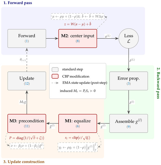
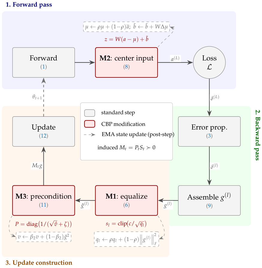
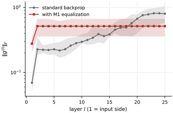
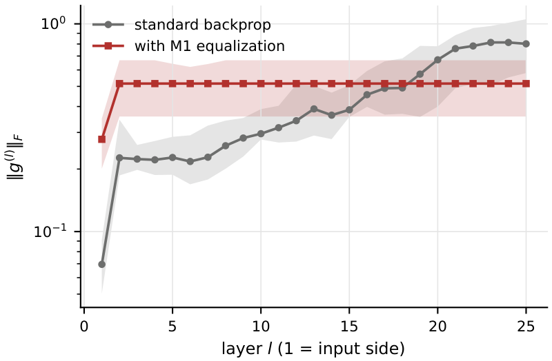
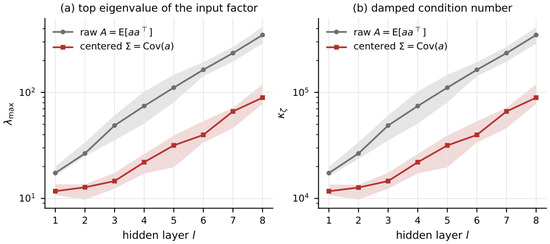
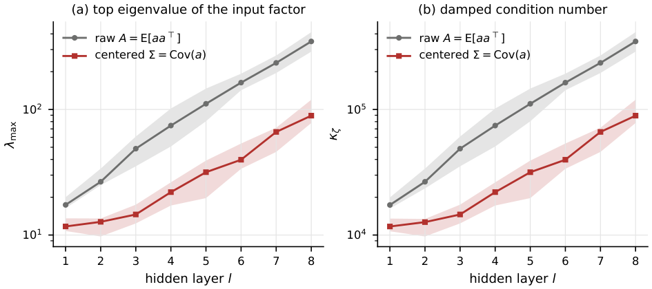
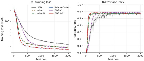
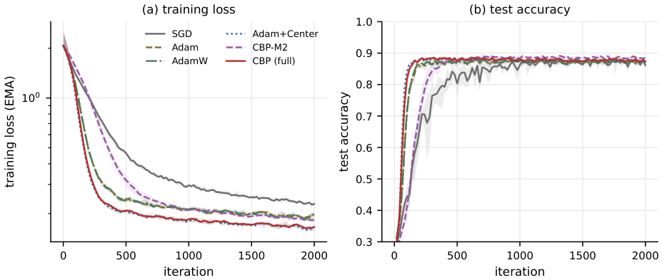
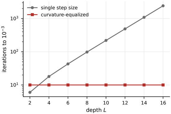
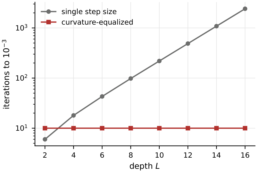
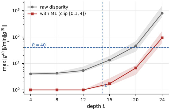
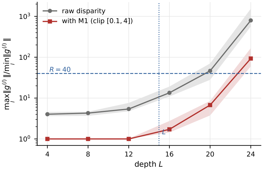
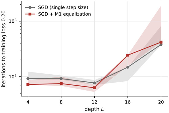
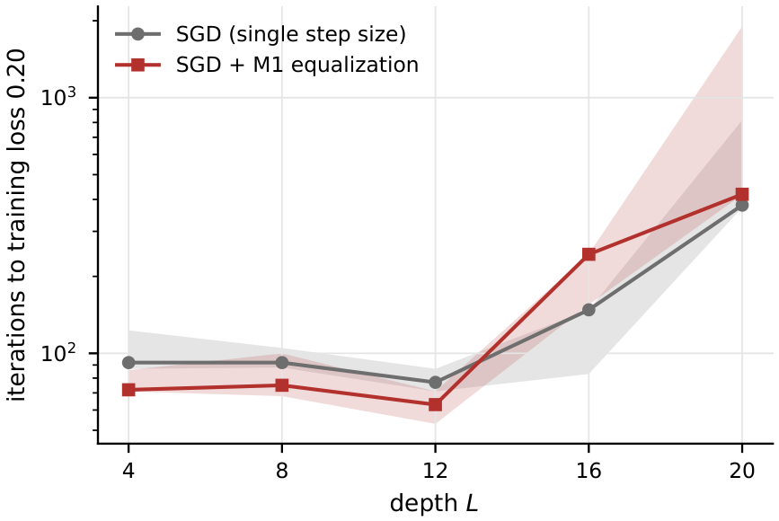

Disclaimer/Publisher’s Note: The statements, opinions and data contained in all publications are solely those of the individual author(s) and contributor(s) and not of MDPI and/or the editor(s). MDPI and/or the editor(s) disclaim responsibility for any injury to people or property resulting from any ideas, methods, instructions or products referred to in the content. |
© 2026 by the author. Licensee MDPI, Basel, Switzerland. This article is an open access article distributed under the terms and conditions of the Creative Commons Attribution (CC BY) license.