


Abstract
Dataset-Based Damage Detection (DBDD) methods are effective for structures with geometric complexity, strong interaction effects, and operational variability, such as liquid-containing tanks with changing fluid levels. In many DBDD applications, accurate damage identification relies on high-fidelity numerical models and extensive simulations across numerous damage scenarios, which results in substantial computational cost. Although finite element modeling is well suited for these problems, fine-meshed models are computationally expensive, whereas coarse-meshed models can introduce errors in extracted dynamic features and reduce damage detection accuracy. This paper proposes an efficient DBDD framework that reduces computational demand while preserving detection reliability. A genetic algorithm is used to select a compact set of highly informative dynamic features that are extracted from a coarse-meshed finite element model and are suitable for training a machine-learning damage classification model. By combining a reduced-cost numerical model with an optimized feature set, the proposed approach decreases simulation time and database storage requirements while maintaining accurate damage prediction. The method is validated on a fluid-filled cylindrical tank under multiple fluid levels, demonstrating robust damage detection performance under simulated response variability (different FEM solvers, mesh sizes, ±5% material perturbations, and SNR 40–10 dB noise). These results indicate that the proposed framework is a practical and accurate solution for structural health monitoring of complex engineering systems.
1. Introduction
Infrastructures play a critical role in ensuring the continuous delivery and distribution of resources across various industries [1,2]. Maintaining their structural integrity is essential for societal resilience, emergency preparedness, and the uninterrupted functioning of modern systems [3]. Consequently, structural health monitoring (SHM) and damage detection have become increasingly important for ensuring the safe and reliable operation of critical infrastructure.
Traditional damage detection techniques, such as visual inspection, ultrasonic testing, and radiographic methods, are widely employed in engineering practice [4,5,6,7,8]. However, these approaches often face limitations in hazardous environments or in structures that cannot be easily taken out of service for inspection [9]. To overcome these limitations, vibration-based damage detection techniques have attracted considerable attention as non-intrusive alternatives capable of identifying structural changes through variations in dynamic characteristics [10]. Despite their advantages, vibration-based approaches encounter several challenges in practical applications. Variations in environmental and operational conditions—such as temperature changes, fluid levels, or operational loads—can significantly influence the dynamic response of structures. These variations may produce changes in measured signals that resemble those caused by structural damage, leading to false damage indications or masking actual damage effects. As a result, distinguishing between operational variability and structural damage remains a fundamental challenge in vibration-based SHM. In recent years, the integration of numerical modeling and data-driven techniques has emerged as a promising approach to address these challenges. In this framework, numerical finite element (FE) models are used to simulate the structural response under different damage scenarios and operational conditions. The simulated dynamic characteristics are then used to construct a database that can be employed to train machine learning (ML) algorithms. Once trained, the ML model can identify damage states in the real structure based on measured dynamic response data. Because the training process relies on simulated datasets generated from numerical models, this strategy is commonly referred to as dataset-based damage detection (DBDD). The DBDD framework offers several advantages for structural systems with complex geometries or operational conditions that are difficult to reproduce experimentally. By using numerical simulations, it becomes possible to generate large datasets representing various damage scenarios and operational states without requiring extensive experimental campaigns. However, the practical implementation of DBDD in complex structures remains computationally demanding. High-fidelity FE models typically contain a large number of degrees of freedom, which significantly increases the computational cost associated with wide-band frequency analyses and the generation of large simulation databases. Moreover, the resulting high-dimensional feature datasets require substantial storage capacity and may reduce the efficiency of machine learning training. Several studies have attempted to improve the efficiency of DBDD frameworks through feature engineering and machine learning techniques. However, many existing approaches rely either on high-fidelity numerical models with considerable computational costs or on automatic feature extraction methods that do not explicitly identify dominant informative features. As a result, opportunities for further efficiency improvements—such as restricting numerical simulations to selected informative frequencies—are often not fully exploited. In addition, the combined impact of model fidelity reduction and feature sensitivity on the robustness of machine learning training has received limited attention, particularly in cases where discrepancies exist between fine-meshed and coarse-meshed numerical models. Therefore, an important research gap exists in the development of DBDD frameworks that simultaneously address computational efficiency, feature sensitivity, and robustness against modeling discrepancies while maintaining reliable damage detection performance. Furthermore, relatively limited studies have investigated such frameworks for fluid–structure interaction problems under varying operational conditions, such as storage tanks with different fluid levels. The objective of this study is to develop a computationally efficient DBDD framework that reduces the cost of database generation while maintaining reliable damage detection performance under varying operational conditions. To achieve this objective, a coarse-meshed (CM) finite element model is employed to construct the simulation database, significantly reducing the computational burden associated with high-fidelity numerical analyses. In addition, a hybrid feature engineering and selection strategy is proposed to identify dominant features that simultaneously exhibit high sensitivity to structural damage and low sensitivity to discrepancies between the frequency response functions (FRFs) obtained from fine-meshed (FM) and CM models. By explicitly identifying informative features, numerical simulations can be restricted to selected frequency points, thereby further reducing computational effort and storage requirements.
The main contributions of this study are summarized as follows:
- Unlike previous DBDD optimizations that either reduce feature dimensionality or use reduced-order models separately, the present framework simultaneously combines a coarse mesh model with a GA-based feature selection that explicitly enforces robustness to FM-CM discrepancies. This dual strategy has not been reported for fluid–structure interaction problems.
- An optimized DBDD framework is proposed that reduces computational cost by employing a coarse-meshed finite element model for database generation while preserving reliable damage localization performance.
- A hybrid feature engineering strategy is introduced to identify features that are simultaneously sensitive to structural damage and robust against discrepancies between fine- and coarse-meshed numerical models.
- An explicit feature selection procedure is implemented to identify dominant informative features, enabling numerical simulations to be restricted to selected frequencies and thereby reducing both simulation cost and database storage requirements.
The proposed framework is applied to a cylindrical storage tank with multiple fluid levels, representing a numerically simulated fluid–structure interaction problem under varying operational conditions. Robustness is evaluated under synthetic noise (SNR = 10–40 dB with Monte Carlo), parametric material perturbations (±5%), mesh variations, and cross-validation between Abaqus and an in-house FEM solver. To evaluate the proposed method, a comprehensive database of simulated damage scenarios is generated under multiple operational conditions. The dataset includes various damage cases and operational states, and it is divided into training and testing subsets to evaluate the generalization capability of the machine learning model. The robustness of the trained model is also assessed under synthetic noise conditions.
2. Related Work
A wide range of vibration-based techniques has been proposed for structural damage detection. These include natural frequency monitoring approaches [11], statistical modeling techniques [12], modal parameter-based methods [13,14,15,16], finite element model updating strategies [17,18], and normalized input power flow methods [19]. Although these techniques have demonstrated promising results in various structural systems, they often face several limitations, including high computational requirements, dependence on specific structural geometries, limited capability for detecting multiple damages, challenges in application to complex three-dimensional structures, and sensitivity to environmental and synthetic noise.
Non-numerical model-based approaches also present several practical challenges. In many cases, identifying both the location and severity of structural damage using only measured response data can be difficult due to the limited information available from a small number of sensors. In addition, collecting experimental data under different operational conditions—such as varying temperatures or fluid levels—can be time-consuming, since the structure must reach each desired operational state before measurements can be taken. These requirements significantly increase the time and cost associated with experimental data acquisition.
To address these challenges, DBDD has emerged as an effective framework for structural health monitoring in complex systems. In this approach, numerical FE models are used to simulate structural responses under multiple damage scenarios and operational conditions, generating datasets that can be used to train machine learning algorithms. Once trained, the ML model can identify structural damage using measured dynamic response data from the real structure. This framework has been successfully applied to various structural systems where environmental and operational conditions significantly influence the dynamic characteristics and may otherwise lead to false damage indications [20,21,22,23,24].
Despite its advantages, the DBDD framework introduces several computational challenges. High-fidelity FE models often contain a large number of degrees of freedom, making the generation of simulation databases computationally expensive. Wide-band frequency response analyses further increase the computational burden because the numerical model must be solved repeatedly across many frequency points. Moreover, the resulting high-dimensional datasets require large storage capacity and may negatively affect ML training efficiency.
To mitigate these challenges, several studies have investigated feature engineering techniques for dimensionality reduction. For example, Seventekidis et al. [25] employed a convolutional neural network (CNN) to automatically extract informative features from structural response data. Although this approach improved damage detection performance, the feature extraction process is performed internally within the neural network, making it difficult to explicitly identify dominant features. As a result, the extracted features cannot easily be reused to reduce simulation effort by restricting numerical analyses to a predefined set of informative frequencies.
To overcome this limitation, Amanabadi et al. [26] proposed an optimized DBDD framework for cylindrical storage tanks with multiple fluid levels using feature engineering and preprocessing techniques. In their approach, a detailed FE model was first used to analyze a subset of damage scenarios and generate a large pool of candidate features. Sensitivity analysis and feature selection techniques were then applied to identify the most informative features. For the remaining damage scenarios, numerical simulations were restricted to computing only these selected features, which reduced the number of impedance matrix solutions required and significantly lowered the overall computational cost. The optimized framework achieved approximately 90% damage detection accuracy while reducing computational cost by 27% and storage requirements by 75% compared with a non-optimized implementation.
Another strategy for improving the efficiency of DBDD frameworks involves reducing the computational complexity of the numerical model itself. In finite element modeling, mesh density directly affects both the accuracy and computational cost of simulations. Fine-meshed (FM) models provide high fidelity but require substantial computational resources, whereas coarse-meshed (CM) models significantly reduce computational effort. However, coarse meshes may introduce discrepancies in the simulated dynamic response, which can negatively affect the performance of machine learning models trained on simulated data.
Bacharidis et al. [27] investigated the use of a reduced-order FE model within a DBDD framework for an aircraft structure and demonstrated that database generation costs could be reduced while maintaining acceptable damage detection performance. However, their validation was limited to a relatively simple structural system with restricted operational variability and a limited number of damage scenarios. Furthermore, because the study primarily relied on automatic feature extraction techniques, it did not investigate the explicit identification of dominant informative features as an additional strategy for reducing computational cost and database storage requirements.
Therefore, despite the significant progress achieved in DBDD research, the combined use of coarse-meshed numerical models and explicitly selected hybrid features for improving both computational efficiency and robustness against modeling discrepancies remains relatively unexplored, particularly for fluid–structure interaction systems operating under varying operational conditions. The present study addresses this gap by developing an optimized DBDD framework that integrates coarse-mesh simulation with hybrid feature engineering and explicit feature selection to achieve efficient and reliable structural damage detection.
3. Materials and Methods
To construct the simulation database required for the proposed DBDD framework, a multi-stage procedure is adopted. It should be noted that the following steps describe only a part of the overall methodology of the study and focus specifically on the generation of the simulation dataset and the extraction of informative features. In the first step, two numerical models of the structure are developed: a fine-meshed (FM) model and a coarse-meshed (CM) model. The adequacy of the FM model is verified by comparing its dynamic responses with experimental results or other validated reference data available in the literature. The CM model is then constructed by reducing the mesh density of the FM model. The mesh density of the CM model is selected such that discrepancies with respect to the validated data remain minimal for several key vibration modes and are within acceptable limits for the remaining modes. In this way, the CM model preserves the overall dynamic behavior of the original structure while significantly reducing computational cost. In practice, achieving this balance typically requires an iterative trial-and-error calibration process. Next, a set of possible structural damage scenarios with relatively high likelihood or significant influence on system stability is identified and denoted as SC_Set. In addition, appropriate sensor locations and harmonic load combinations are selected in order to maximize the sensitivity of the measured responses to the targeted damage scenarios. For structures with similar configurations, these sensor and excitation layouts can often be adopted from previously reported studies. The number of sensor locations is denoted by , and the number of load combinations by .
Since the proposed framework relies on machine learning techniques, the generated simulation data must later be divided into subsets serving different purposes, such as feature identification, model training, and performance evaluation. In many machine learning studies, a common practice is to allocate approximately 70% of the available data for model development (training and validation) and the remaining 30% for testing in order to evaluate the generalization capability of the trained model. Following this widely adopted practice, the damage scenarios in SC_Set are divided into three non-overlapping subsets. Specifically, 40% of the scenarios are randomly selected and denoted as , while 30% are stored as . The remaining 30% of the scenarios form . Consequently, the combined size of and corresponds to 70% of the total scenarios, which are used during the dataset preparation and model development stages, whereas is reserved for the final evaluation stage of the framework. For the damage scenarios included in , the frequency response functions (FRFs) measurable at the selected sensor locations under the defined harmonic load combinations and different operational conditions (OCs) are computed using the validated FM model. The obtained responses are stored in a database referred to as FM_Dataset. This dataset serves as a high-fidelity reference for the subsequent feature engineering process. The frequency analysis for each operational condition is performed within the interval with a frequency step size of , where denotes the first natural frequency of the intact structure under the -th operational condition . Parameter is preferably selected within the range 0–0.5 in order to preserve useful low-frequency information, which typically contains global structural response characteristics and is often highly sensitive to structural damage. Parameters and are determined based on the characteristics of the structural system, the expected excitation energy distribution, and the considered damage scenarios.
To obtain a sufficiently detailed representation of the FRF while keeping the dataset size manageable, the frequency step size is selected so that approximately 1000 frequency points are sampled within the selected frequency interval. In many practical cases, this requirement can be satisfied using the relation , which distributes the frequency samples uniformly across the defined band. Accordingly, 1000 features are extracted from each FRF, providing a sufficiently dense representation of the dynamic response. This feature resolution is consistent with the level of accuracy achieved in the study [26] and forms the basis for the subsequent feature engineering and feature selection procedures used in the proposed framework.
The extracted features are then ranked using multiple feature selection techniques. These include standard deviation (as an unsupervised method [28,29]) and several supervised methods, namely Random Forest (RF) [30], Classification and Regression Trees (CART) [31], and Extreme Gradient Boosting (XGB) [32]. These algorithms have proven successful in related studies and demonstrate strong performance for this type of problem [22,26].
To evaluate sensitivity, a classification framework based on a neural network, with hyperparameters tuned for the problem domain [22], is implemented. Using 10-fold cross-validation, predictive accuracy is assessed by progressively including the top-ranked 20%, 22.5%, 25%, 27.5%, and 30% of features from each ranking method. The feature subset that yields the highest predictive performance (therefore indicating maximal sensitivity to the damage scenarios) is retained to form a refined dataset denoted as . The number of selected features is denoted as . In addition, normalized feature-importance scores are stored in a dictionary, FM_iFr_dic, which maps each feature’s normalized importance to its original index in the raw feature vector.
Subsequently, for the same scenarios in , FRFs at the sensor locations under the selected load combinations and various OCs are computed using the CM model over the same frequency range and with the same . These results are stored as CM_Dataset. For each of the 1000 extracted features, the difference between the values in CM_Dataset and FM_Dataset is computed. Features are then ranked based on the inverse of the mean squared error (MSE), such that the smallest MSE corresponds to the highest importance. In this way, highly ranked features are those least sensitive to numerical discretization. The top features are then retained, and their normalized importance scores are stored in a second dictionary, CM_iFr_dic, following the same convention as above.
The next phase is to determine an optimal feature subset, denoted as iFr_set, by combining information from FM_iFr_dic and CM_iFr_dic. The goal is to select features whose values from CM_Dataset can be used to train the tuned classification model such that it can accurately predict damage scenarios when evaluated using the corresponding feature values in FM_Dataset. Because the number of possible feature combinations is extremely large, an exhaustive search is computationally infeasible.
To address this, a genetic algorithm (GA) is adopted and modified to match the requirements of the present problem. First, a new dictionary, iFr_dic, is constructed by intersecting the feature indices contained in FM_iFr_dic and CM_iFr_dic. The number of entries in iFr_dic is denoted as gene_size. The GA uses binary chromosomes of length gene_size, where a value of 1 indicates inclusion of the corresponding feature and 0 indicates exclusion. The number of selected features in a chromosome is denoted as , and the corresponding indices in the original raw dataset are retrieved via iFr_dic. The GA fitness function is defined as the inverse of the prediction accuracy for the damage scenarios, evaluated using the tuned classification algorithm. Specifically, the model is trained using feature values from CM_Dataset and tested using the corresponding features from FM_Dataset for the scenarios in . The GA output is genetic_iFr_set, which contains the indices of the selected features with respect to the original raw dataset.
Several strategies are employed to accelerate GA convergence. First, the search space is reduced by constraining to a practical interval, typically from to . Second, the normalized feature-importance values from FM_iFr_dic and CM_iFr_dic are used as prior knowledge to guide the search, based on the assumption that features with higher importance in either dictionary are more likely to appear in the final subset. In this study, three guidance mechanisms are investigated: (1) using the normalized importance ratios as probabilities for feature inclusion when generating the initial population; (2) incorporating these ratios into the mutation operator; and (3) a hybrid strategy combining both mechanisms. Incorporating this prior information improves GA efficiency and accelerates convergence of the overall framework.
After selecting genetic_iFr_set, the corresponding feature values from FM_Dataset are extracted and stored in Train_Dataset. Next, the scenarios in are simulated using the CM model, but only for the features in genetic_iFr_set, and these results are appended to Train_Dataset. This consolidated Train_Dataset is then used to train the classification algorithm. Finally, predictive accuracy is assessed using measured data from the real structure corresponding to the selected features.
Compared with conventional DBDD workflows, the proposed framework incorporates the CM model during database construction for the scenarios included in . This design allows part of the database generation process to be performed using a lower-fidelity model while maintaining consistency with the high-fidelity simulations used in . In addition, instead of performing impedance-matrix inversions over the entire frequency grid, the computations are carried out only at the selected feature locations identified during the feature engineering stage. Consequently, the database is constructed using a reduced set of frequency-domain response components. This formulation also leads to a lower-dimensional feature representation for the subsequent classification model.
The proposed method for optimizing damage detection within the DBDD framework is implemented in nine steps:
- Generate using and the FM model.
- Generate using and the CM model.
- Apply hybrid feature selection and sensitivity analysis to FM_Dataset to construct FM_iFr_Dic.
- Compute STD-based feature importance using and to construct CM_iFr_Dic.
- Initialize the GA population using information from FM_iFr_Dic and CM_iFr_Dic.
- Run the GA with the tuned decision-tree (DT) ensemble to minimize the cost function and obtain Genetic_iFr_Set.
- Extract features from using Genetic_iFr_Set to build Part 1 of Train_Dataset.
- Complete by analyzing with the CM model using Genetic_iFr_Set, then train the tuned deep neural network (DNN) ensemble.
- Construct by analyzing with the FM model using Genetic_iFr_Set, then predict using the trained DNN ensemble and compute the final accuracy.
A flowchart summarizing these steps is provided in Figure 1. The processes associated with each step are indicated by arrows of the same type (color and style), as defined in the legend at the top of the figure.
Figure 1.
Flowchart of the proposed optimized DBDD method. STD: standard deviation; RF: random forest; CART: classification and regression trees; XGB: extreme gradient boosting. Arrow styles indicate process types, as defined in the legend.
3.1. Computational Cost Analysis of the Proposed Method
Three general approaches can be identified for constructing the database used in the DBDD method:
(1) The conventional approach, which employs a comprehensive numerical model to extract the full set of dynamic features under a wide range of damage scenarios;
(2) The optimized approach proposed in a previous study [22], in which only a subset of features is targeted during numerical analyses to reduce the size of the dataset;
(3) The optimization strategy introduced in the present study.
The computational cost of these three approaches is evaluated using a parametric formulation. This simplified parametric calculation is adopted to enable a transparent, like-for-like comparison across the methods and to clarify the expected reduction in cost achieved by the proposed framework. The notation used in the equations of this section is summarized in Table 1.
Table 1.
Summary of notations and their definitions used throughout the study.
The total computational cost for Method 1, , is assumed to be dominated by two components: (i) database construction and (ii) training of the DBDD classification algorithm, while other processing times are considered negligible in comparison. This time is expressed as a function of the number of damage scenarios, excitation load combinations, environmental conditions, training data ratio, number of dynamic features, the impedance-matrix analysis time per scenario, and the time required to train the deep learning model using the prepared training data, as shown in the following equation:
In the above equation, denotes the total training time of the DNN algorithm. This time is assumed to be proportional to the number of database samples, with representing the training time per sample (or, equivalently, a normalized baseline training time). Accordingly, the total time required to perform damage detection using Method 1 of the DBDD approach can be written as a function of , where is the time required to construct the training database in Method 1.
For Method 2, the computational cost associated with database construction is divided into three components. The first component is the time required to generate the initial portion of the database using the numerical model evaluated over the full set of dynamic features. The second component corresponds to the time required for feature engineering and sensitivity analyses to identify the most important features and determine their optimal number. The third component is the time required to generate the remaining portion of the database using the numerical model evaluated only for the selected top features. Therefore, the total time for Method 2, , can be expressed as follows:
In simplified form, the total time required for Method 2 can be expressed as a multiple of . Consequently, the time saved by adopting Method 2 relative to Method 1 is obtained by subtracting the total time of Method 2 from that of Method 1, yielding the optimized time as follows:
This method provides a net time saving when the following condition is satisfied:
For complex structures with a large number of degrees of freedom (DOFs), the ratio typically approaches zero, and the maximum achievable time saving approaches .
The third method proposed in this study consists of five computational components. Components (2) and (4) are identical to those in Method 2. In Component (1), the computational time required to extract the features for using the CM model is added to the cost formulation of Method 2. Component (3) represents the time required to construct the supplementary database, which depends on the CM-model analysis time and the number of optimally selected features specific to Method 3. In addition, Method 3 includes a fifth component that accounts for the time required to perform feature selection using a metaheuristic optimization algorithm, namely a genetic algorithm (GA). Accordingly, the total execution time for Method 3, , can be expressed as follows:
The optimized (saved) time can be calculated by subtracting from the total time required for Method 1, . For complex structures with a high number of DOFs, the ratio tends toward zero, and the maximum achievable time saving approaches . Accordingly, Method 3 becomes more efficient than Method 2 provided that the following condition is satisfied:
The maximum time saving achievable by Method 3 occurs as and can be written as . To achieve 99% of this maximum saving, a minimum threshold value for is defined as follows:
Values of below this threshold result in a time-saving reduction of less than 1%; however, such small values can substantially degrade the numerical model’s accuracy and compromise the reliability of the DBDD method.
3.2. Data-Driven Modeling Techniques
This study employs Deep Neural Networks (DNNs) and Decision Trees (DTs) to learn the relationship between engineered features and damage scenarios within the proposed optimized DBDD framework. DNNs, which comprise multiple interconnected layers, are well suited to capturing complex and nonlinear feature representations, enabling accurate prediction of damage levels.
The complete dataset (10 vertical levels × 8 angular sectors × 2 severity levels, including single- and double-damage scenarios) was randomly split into training (50%), validation (20%), and test (30%) sets using a fixed random seed (42) for reproducibility. Stratification was applied to preserve the proportion of each damage scenario across all splits. No data leakage occurred because all samples from a given damage configuration (same level, sector, severity, and mesh/solver combination) were kept within the same split. The test set was used only once for final evaluation. Class distribution was moderately balanced; the smallest class contained approximately 85% of the samples of the largest class. To address any residual imbalance, class weights inversely proportional to class frequencies were used during training. Specifically, the weight for class was set as , where is the total number of training samples, is the number of classes, and is the number of samples of class .
For vertical level (10-class) and severity (2-class) prediction, a DNN with five hidden layers (100 neurons each, ReLU activation) was employed. For angular sector (8-class) prediction, a pseudo-bagging ensemble was used as described below. Each DNN was trained using categorical cross-entropy loss, the Adam optimizer (learning rate = 0.001), and a batch size of 32. To prevent overfitting, early stopping with a patience of 15 epochs (monitoring validation loss) was applied, together with L2 regularization (weight decay = 0.0001) and dropout (rate = 0.3) after each hidden layer. The hyperparameters were optimised via a grid search using the validation set, following the approach in [22]. A softmax activation function was used in the output layer for multi-class classification. Ten-fold cross-validation was performed on the training set to assess feature sensitivity, and the final model was retrained on the full training set. In addition to accuracy, we report macro-F1 and balanced accuracy (average of recall per class) to account for any class imbalance.
The proposed DBDD method predicts three independent damage attributes: vertical elevation (10 classes), angular sector (8 classes), and damage severity (2 classes: low or high). For each attribute, a separate DNN is trained using the same feature engineering and hyperparameter optimisation described above, with one exception. For angular sector prediction, the inherent symmetry in sensor placement, excitation points, and tank geometry causes poor accuracy when all sensor data are used together. Therefore, a pseudo-bagging ensemble is employed: the dataset is partitioned by sensor location and excitation, features are engineered per subset, and multiple DNNs are trained; the final sector prediction is obtained by majority vote. The architecture of this ensemble is detailed in our previous work [26] (Figure 1). For vertical level and severity prediction, a single DNN is sufficient. In the following section, we present detailed results for vertical level prediction. Results for the angular sector and damage severity are then summarized to demonstrate full localization and severity assessment. All three predictions together uniquely identify the damage state.
In parallel, a DT model was employed to rapidly map the key features selected by the Genetic Algorithm to the corresponding damage scenarios. The DT was selected primarily for its computational efficiency, which is critical when it is embedded in the GA cost function and must be evaluated repeatedly. Its hyperparameters were also tuned via grid search on the validation set to balance predictive performance and runtime. The final DT configuration used , , minimum samples per leaf and split of 0.005, the squared error criterion, and the best splitter.
3.3. Numerical Modeling for Structural-Fluid System
Numerical modeling of a coupled structural–fluid system involves formulating and solving the governing differential equations in both the structural and fluid domains using the finite element method (FEM). The structural domain is typically described by the equations of motion, here written assuming zero damping. This assumption is justified because the tank structural material (similar to steel) has a very low loss factor (<0.005). A sensitivity analysis compared FRFs with and without Rayleigh damping (ζ = 0.002) and found that the selected feature values changed by less than 2%, which did not alter the final damage classification. Therefore, zero damping is retained for computational efficiency. The fluid domain is governed by a complex wave equation that can be simplified through standard assumptions such as fluid compressibility, homogeneity, and non-viscosity [33]. The governing equations are discretized using variational principles together with Green’s theorem, yielding matrix equations that represent nodal interactions within each domain. At the fluid–structure interface, compatibility and equilibrium conditions couple the two fields by relating the fluid pressure to the structural acceleration. Additional phenomena, such as surface-wave effects, can be incorporated when necessary; however, they are commonly neglected when their influence on key dynamic characteristics, such as natural frequencies, is minimal [34].
The fluid-filled cylindrical tank is modeled using a coupled finite element formulation in the frequency domain. For the structural domain, the undamped dynamic equation is , where and are the structural mass and stiffness matrices, is the displacement vector, and is the external force. For the fluid domain, assuming compressible, inviscid, and irrotational flow, the governing wave equation reduces to , with the fluid pressure and the speed of sound. Discretizing the fluid domain with finite elements gives , where and are the pseudo-mass and pseudo-stiffness matrices, and accounts for boundary conditions (detailed derivations of , , and the coupling matrix are given in Equations (3)–(7) of our previous work [26]). At the fluid–structure interface, continuity of normal acceleration imposes . Surface wave effects are neglected because they have a negligible influence on the frequency range of interest (0.8–2.5 times the first natural frequency) [26]. The FEM results obtained without surface wave effects were successfully validated against experimental data for the intact tank, showing good agreement. Therefore, the simpler boundary condition is adopted, which is consistent with the validated model.
Assembling the structural and fluid equations leads to the following coupled system for harmonic excitation :
The frequency response function (FRF) matrix is therefore [35]:
For a damaged structure, the stiffness matrix is replaced by (obtained by reducing the Young’s modulus or thickness of damaged elements according to each scenario), while the fluid matrices remain unchanged. The FRF matrix for the damaged case, , follows the same form with in place of (see Equation (11) in [26]). The coupled system is solved using an in-house Fortran code that implements the Skyline method [36], which is efficient for repeated analyses across frequencies and damage scenarios. The code was validated against analytical solutions and experimental data from literature, as reported in [26].
To efficiently solve the coupled system, a Fortran-based FEM code implementing the Skyline method was developed [36]. This implementation is particularly effective when repeated analyses are required for different fluid levels and multiple damage scenarios. For damaged configurations, the mass and stiffness matrices are modified accordingly, and new FRFs are computed. By comparing FRFs obtained under different operational conditions and damage states, changes in the dynamic response can be quantified and used as indicators of structural damage, supporting diagnosis within the structural health monitoring framework.
4. Case Study
To implement the proposed optimized DBDD framework, the cylindrical fluid-filled tank investigated by Chiba et al. [37] was selected because validated experimental data are available for model verification. Figure 2 illustrates the tank geometry and the corresponding experimental test setup. The tank has a radius mm, shell thickness mm, modulus of elasticity GPa, Poisson’s ratio , and structural material density kg/. The overall tank height is mm, which results in the geometric parameter .
Figure 2.
Filled-tank geometry (adapted from authors’ previous work [26]).
4.1. Sensor and Excitation Node Configuration
The selection of sensor and excitation locations is a key factor governing the performance of the DBDD method. Although structural damage can, in principle, affect the dynamic response associated with any excitation point, the magnitude and observability of that effect depend strongly on the excitation location and the participating vibration modes. For damage detection in the cylindrical tank, two excitation points and four sensor placements were adopted following the configuration reported in [38]. They were chosen to provide representative and sufficiently rich measurements of the structural response (Figure 3).
Figure 3.
(a) Planar arrangement of sensor and excitation points, along with angular sectioning for analysis. (b) Vertical arrangement of sensor and excitation points, along with vertical partitioning of the tank into discrete levels (adapted from authors’ previous work [26]).
Two excitation strategies were considered. In the first strategy, points 1 and 2 were excited with a phase difference of (LC2). In the second strategy, points 3 and 4 were excited in phase (LC3). Using multiple load combinations allows the damage-induced changes in the FRFs to be observed from different excitation perspectives, which improves sensitivity and increases the robustness of the overall detection framework.
4.2. Damage Scenarios
In the DBDD method, damage identification accuracy depends strongly on the quality and diversity of the training database. Although the framework can, in principle, accommodate a wide range of damage cases, including single and multiple damages with different locations and severities, generating a dataset that exhaustively covers all combinations quickly becomes computationally prohibitive. To manage this challenge while limiting the loss of accuracy as model complexity increases, this study adopts an element-grouping strategy for the cylindrical tank. The objective of the case study is to determine the predefined vertical level at which damage occurs.
As shown in Figure 3, the tank shell is partitioned into 80 element groups by dividing the structure into ten vertical levels and eight angular sectors. Each angular sector spans 45°, starting from excitation node 1 and proceeding clockwise. Using this grouping, 1280 damage scenarios are defined by combining ten vertical levels, eight angular sectors, and two damage severities (30% and 60%). It is important to note that damage severity is treated as a binary classification (low: 30% thickness reduction; high: 60% reduction) rather than a continuous regression. The scenario set also includes cases with one or two simultaneous damages within the same vertical level, with potentially different severities. To represent operational variability, four distinct water levels are considered for each damage scenario. In each simulation, two excitation load cases are applied simultaneously. As a result, 5120 frequency-domain finite element analyses are performed, producing a database that captures the full range of defined damage and operational conditions.
Damage scenarios are identified using a compact notation that specifies the vertical level, angular sector, and damage severity. In this notation, the letter L indicates the vertical level of the tank shell, T denotes the angular sector where the damage occurs, and the number in parentheses represents the percentage of thickness reduction. For example, the label L4T45(30) indicates a damage scenario in which a 30% thickness reduction is applied to all elements located at vertical level 4 within the angular sector extending from 0° to 45°. When two damages occur simultaneously within the same level, both sectors and their corresponding severities are included in the notation. For instance, L4T45(30)T135(60) represents two damages at level 4: a 30% thickness reduction in the 0–45° sector, and a 60% thickness reduction in the 90–135° sector.
For completeness and to enable consistent comparisons, the full set of 5120 analyses is used to construct the complete database; however, subsets of this database are then selected and utilized according to the proposed DBDD workflow described in the methodology.
4.3. Numerical Model
The finite element method (FEM), as described in the Methodology section, was used for numerical modeling of the coupled structural–fluid system. The fine model (FM) was developed using 288 four-node S4R shell elements and 2016 eight-node AC3D8 acoustic elements for each 5% increment of shell and fluid height. Over the full tank height, this discretization results in 40,320 fluid elements and 5760 shell elements. The coarse model (CM), constructed following the procedure described in the previous section, employs 72 four-node S4R elements and 504 eight-node AC3D8 elements per 5% increment of shell and fluid height. The coarse mesh was generated by systematically removing every second node in each direction, which inherently preserves element shape because the original fine mesh had good aspect ratios. A visual inspection confirmed no distorted elements. Quantitative checks confirmed that aspect ratios remained well below 5 for all shell elements and that Jacobian determinants for acoustic elements were positive, satisfying standard finite element quality criteria. Based on the resulting reduction in model size, and accounting for the effect of boundary conditions and other factors on the total number of degrees of freedom (DOFs), the ratio is approximately (Figure 4). To explore the limits of mesh coarsening, a preliminary study was conducted with an even coarser mesh (ξ ≈ 1/50, i.e., 50% fewer elements than the current CM). The FRF discrepancies relative to the FM model increased significantly, leading to a drop in damage detection accuracy of approximately 18% for clean data and 21% for noisy data (SNR = 20 dB). This non-linear degradation suggests that the current CM (ξ ≈ 1/27) represents a practical boundary where computational gain is achieved without sacrificing reliability. Beyond this point, further coarsening causes rapid loss of feature discriminability, particularly for high-frequency modes sensitive to local damage.
Figure 4.
Finite element model for : (a) fine mesh; (b) coarse mesh. Blue indicates water; gray indicates tank structure.
Table 2 lists the first five natural frequencies of the tank computed using the FM model for several fluid height levels. Here, denotes the height-to-length ratio . Figure 5 compares the FM results obtained in this study with those reported in [38], indicating satisfactory agreement and validating the adopted numerical modeling. In Figure 5, and denote the circumferential and longitudinal mode numbers, respectively. The CM predictions are also shown using black square markers. The separation between the FM (red markers) and CM (black square markers) illustrates the discrepancy introduced by the coarser discretization.
Table 2.
First five modal frequencies of the tank for different fluid level ratios () based on the FM model.
Figure 5.
Comparison of natural frequencies for a cylindrical tank () with varying (colored lines and cross markers represent analytical and experimental results reported in Chiba et al. [38]; red square markers: FM model results; black square markers: CM model results).
The dynamic responses of the FM and CM models were compared using the FRFs recorded at sensor 1 for both the intact configuration and the damaged case under the partially filled condition . Figure 6 shows the FRFs evaluated over a frequency range from 0.8 to 2.5 times the fundamental natural frequency of the intact structure. This normalized frequency ratio is shown on the horizontal axis and is sampled at 1000 discrete points, which constitute the raw features. The vertical axis represents the logarithm of the absolute value of the radial displacement amplitude measured at the sensor location.
Figure 6.
FRFs from sensor 1 under simultaneous load cases LC1 and LC2, comparing the intact and damaged tank at for both the FM and CM models.
The corresponding absolute peak frequencies (Hz) can be obtained by multiplying the dimensionless peak locations by the fundamental natural frequency of the intact quarter-filled tank given in Table 2 (188.34 Hz). The datasets used in this comparison, consistent with Steps 1 and 2 of the Methodology section, were generated using the FM and CM models, respectively.
4.4. Synthetic Noise and Cross-Model Uncertainty Injection
Because experimental FRFs for damaged states are unavailable, we generate a synthetic test set that mimics realistic measurement imperfections and modelling variability while remaining fully numerical. For each damage scenario, the base FRF is computed either with Abaqus or with an in-house Fortran FEM code (chosen randomly, half from each solver), using one of three different mesh sizes: coarse, medium (element count between coarse and fine), and fine; the mesh size is also selected at random for each sample. To simulate material uncertainty, we perturb the key properties—Young’s modulus E, structural density , and water density —independently by ±5% uniform random variation. Then, white Gaussian noise is added to the FRF amplitudes at signal-to-noise ratios (SNR) of 40, 30, 20, and 10 dB. Here, SNR is defined as , where the noise is zero-mean additive white Gaussian applied independently to the real and imaginary parts of each frequency line of the FRF. For each SNR level, the noise injection is repeated 50 times (Monte Carlo) to produce a distribution of corrupted FRFs. Throughout the rest of the paper, we refer to this combination of solver switching, mesh size variation, property perturbation, and additive noise as our synthetic noise assumption. Frequency-dependent noise, sensor bias drift, and operational variability beyond water level changes are not modelled here; their inclusion is left for future work.
4.5. Prediction Framework for Damage Localization and Severity
As detailed in Section 3.2, the proposed method predicts three independent damage attributes (vertical level, angular sector, and severity) using separate DNNs—with a pseudo-bagging ensemble for angular sector prediction. The performance of this prediction framework is evaluated in Section 4.10.
4.6. Feature Engineering on DBDD Method Efficiency and Accuracy
As described in Steps 3 and 4 of the methodology, feature-importance techniques were applied to identify the most salient features, with the objective of reducing database storage requirements and lowering the computational cost of FEM analyses. Four feature-importance methods were examined for the FM model, including one unsupervised method (standard deviation) and three supervised methods (Random Forest, CART, and XGBoost). For the supervised methods, feature rankings were evaluated using a DNN trained on with 10-fold cross-validation. The optimal number of features was then determined through the sensitivity analysis procedure shown in Figure 1. The resulting selected subset is referred to as the Total Used Features (TUF).
To assess robustness, the trained model was also evaluated on unseen data contaminated with a synthetic noise assumption (noisy_Test_Data), and the resulting damage detection accuracy was compared with the corresponding accuracy obtained using clean test data. For the unsupervised method, the initial supervised ranking step was not required; however, the remaining evaluation and sensitivity-analysis procedures were kept consistent to enable a fair comparison.
The results are summarized in Figure 7, which shows damage detection accuracy (Macro F1) as a function of the selected feature percentage for each method. For the unsupervised standard deviation method, 30% of the features were sufficient to achieve accurate damage prediction. Among the supervised methods, CART provided the best performance, achieving accuracies of 92.46% and 87.72% for clean and nois_Test_Data (20 dB), respectively, while using only 27.5% of the original features (275 features). The top-ranked CART features were stored in FM_iFr_Dic. Subsequently, the standard deviation method was applied to both and , and the top 275 features with the lowest discrepancy were stored in CM_iFr_Dic.
Figure 7.
Comparison of the damage detection accuracy of a DNN trained using optimal feature subsets selected by various feature-importance methods versus a DNN trained using all 1000 features.
4.7. Genetic Algorithm Overview and Hyperparameter Tuning
Genetic algorithms (GAs) are evolutionary optimization methods inspired by natural selection. They search for optimal or near-optimal solutions by iteratively evolving a population of candidate solutions using selection, crossover, and mutation operators. The process begins with an initial population. In each generation, the fittest individuals are preferentially selected to produce offspring, crossover recombines parental information, and mutation introduces controlled randomness to maintain diversity. The evolution continues until a stopping criterion is met, such as reaching a maximum number of generations or attaining a target fitness value.
To implement Steps 5 and 6 of the methodology, a GA was used to identify an optimal combination of top-ranked features drawn from the previously constructed FM_iFr_Dic and CM_iFr_Dic. Specifically, the top 100 features from each dictionary were pooled to form Genetic_iFr_Dic (200 candidate features in total). The threshold of 100 features was determined empirically. A sensitivity study varied the number of retained features per dictionary from 50 to 200. Retaining fewer than 80 features reduced macro F1 by more than 3%, while retaining more than 120 provided less than 0.5% improvement but increased the GA gene_size (and thus computational cost) proportionally. Therefore, 100 features per dictionary strikes an optimal balance between classification accuracy and efficiency. Then the GA searched for the feature subset that maximised classification performance. Because a Decision Tree (DT) provides acceptable predictive accuracy while requiring substantially less computational time than a DNN [22], the DT model was used to evaluate the GA cost function. A potential concern is that features selected using a DT as the fitness function may not be strictly optimal for the final Deep Neural Network (DNN). To mitigate this risk, we verified that the selected feature subsets yield consistent ranking trends when evaluated with a lightweight DNN (one hidden layer) on a small validation set. The DT-selected features achieved approximately 98% of the accuracy of a DNN-based selection but at a fraction of the computational cost. Moreover, the GA’s fitness function could be replaced by a DNN in future work if computational resources permit. For the present framework, the DT provides a pragmatic balance between search efficiency and near-optimal feature selection, as evidenced by the final DNN’s strong performance (≥90% macro-F1 for clean data).
The performance of a GA is strongly affected by its hyperparameters, including population size, tournament size, mutation rate, crossover method, crossover rate, and mutation method. Population size controls how many candidate solutions are explored at each generation and therefore influences the trade-off between exploration and computational cost. Tournament size determines selection pressure, affecting convergence speed and the likelihood of premature convergence. Mutation rate and mutation method promote diversity and help the search avoid stagnation, while crossover rate and crossover method govern how parental information is combined and thus influence the balance between exploration and exploitation. For the present problem, these hyperparameters were tuned using a grid-search procedure.
The grid search evaluated population sizes of [100, 200, 500], tournament sizes of [2, 3, 5, 7], mutation rates of [0.01, 0.05, 0.1], and crossover rates of [0.7, 1.0]. Two crossover operators (crossover_one_point and crossover_uniform) and two mutation operators (mutate_swap and mutate_random_reset) were tested using the random_unique initialization method. For consistency across experiments, the number of generations was fixed at 200. Figure 8 summarizes the influence of these hyperparameter combinations on optimization accuracy; the crossover and mutation operators are denoted as options 1 and 2, respectively.
Figure 8.
Effect of GA hyperparameters on accuracy over 200 generations.
As shown in Figure 8, population sizes in the range of 100 to 500 have a limited effect on accuracy for most configurations, except when using mutate_swap, where intermediate population sizes reduce performance. Increasing tournament size consistently improves accuracy, particularly when combined with the selected mutation operator and crossover rate. Higher mutation rates generally reduce accuracy, whereas changes in crossover rate have a comparatively minor impact. Across all combinations, the crossover_one_point operator yields higher accuracy than crossover_uniform.
Based on the grid-search results, the best-performing GA configuration used a population size of 500, tournament size of 7, mutation rate of 0.01, crossover method one_point, crossover rate of 1.0, and mutation method random_reset, achieving a best fitness score of 91.36. However, a population size of 100 produced a nearly identical accuracy (91.33%) while requiring substantially lower computational cost. Therefore, a population size of 100 was selected as the most efficient setting for the subsequent analyses. Figure 9 presents the fitness evolution over generations using the tuned hyperparameters and shows an approximately 20% improvement (%72.5 to %91.4) in accuracy obtained through GA-based optimization of the Genetic_iFr_Dic feature set.
Figure 9.
Fitness improvement over generations using tuned GA hyperparameters.
Figure 10 illustrates the optimal feature locations selected by the GA and stored in Genetic_iFr_Dic. In the FRFs of the intact and damaged configurations obtained from the FM model, the selected features are marked as vertical lines, with blue lines denoting features chosen from and green lines denoting features chosen from . This visualization identifies the frequency regions that are most informative for distinguishing damage levels in a partially filled cylindrical tank, including cases with one or two simultaneous damages within a given vertical level. As shown in the figure, the selected features are distributed across various frequency ranges and are not confined to a single band. Furthermore, the majority of selected features are located away from the resonance peaks, which reduces the influence of damping on the performance of the proposed method.
Figure 10.
GA-selected features (blue: selected from ; green: selected from ) overlaid on the FRFs of the intact and damaged FM models, highlighting key frequency regions for damage detection in a partially filled cylindrical tank.
4.8. Dataset Completion Using
Following Steps 7–9 of the methodology described in Section 3, the training and test datasets were completed using the feature indices stored in Genetic_iFr_Set. First, the corresponding feature values were extracted from FM_Dataset (generated with the fine-mesh model for to form Part 1 of Train_Dataset. To complete the Train_Dataset, the coarse-mesh (CM) model was used to simulate the scenarios in , but the analysis was restricted only to the frequency points specified by Genetic_iFr_Set. The resulting responses were appended to Train_Dataset. Finally, for the unseen test scenarios (), the fine-mesh (FM) model was used—again limited to the same selected frequency points—to build Test_Dataset. Because the FM model had been validated against experimental data (Section 4.3), Test_Dataset serves as a representative proxy for measured structural data. The tuned DNN was then trained on the completed Train_Dataset and evaluated on Test_Dataset. The final classification accuracy is reported in Section 4.10.
4.9. Computational Cost Analysis
A key contribution of this study is the development of an efficient database-generation strategy for damage detection within the DBDD framework. To quantify the computational cost, a comparative assessment was performed using one verified FM and one verified CM from the case study. The comparison considered CPU utilization, RAM usage, and the total computational time required for frequency-domain analysis over 1000 frequency steps, sufficient to generate the complete FRF for a single damaged scenario. All simulations were conducted on a workstation equipped with an AMD Ryzen 7 7735HS processor(8 cores, 4.75 GHz (AMD, Santa Clara, CA, USA) and 32 GB DDR5 RAM.
As shown in Figure 11, CPU utilization is similar for both models; however, the FM model requires substantially more RAM because of the larger system matrices. The CM completes the analysis in approximately 79 s, whereas the FM requires approximately 2210 s, corresponding to . To demonstrate the optimization potential of the proposed DBDD framework for complex structures, the parametric values were selected based on this case study. Two non-overlapping subsets comprising 40% and 30% of were randomly selected and denoted as and , respectively. Because 70% of is used for training, the ratio of to the training set is .
Figure 11.
CPU and RAM usage during FM and CM frequency-domain analyses at over 1000 frequency steps (0.8–2.4 the fundamental frequency) to obtain the complete FRF. Simulations were run on a PC with an AMD Ryzen 7 7735HS (8 cores, 4.75 GHz) and 32 GB DDR5 RAM.
In addition, was taken as 0.25, representing the average value obtained from the sensitivity analysis described in the Methodology section, where predictive accuracy was evaluated by progressively including the top 20%, 22.5%, 25%, 27.5%, and 30% of features ranked by the various feature-selection techniques. The parameters , , and were set to 4, 5, and 10, respectively, consistent with the methodology.
Based on the training sample size, the tuned DNN training time per fold, and the FM timing reported by Amanabadi et al. [22,26], the values s and s were adopted. Because operational variability can influence the number of effective DOFs, is considered an average value. Substituting these parameters into Equation (3) yields an estimated optimization time for Method 2 of approximately . Accordingly, Method 2 is expected to provide a net benefit when s, as indicated by Equation (4).
Genetic algorithm parameters were set to and , consistent with the grid-search results. The DT processing time, , was estimated as 2 s for classification on 10,240 samples (the first training subset) with (250 features). Using the mean accuracy obtained from 5-fold cross-validation with the DT as the GA cost function, the cost-evaluation time was estimated as s. Table 3 summarizes the parameter values adopted from the case study, which yield s using Equation (1).
Table 3.
Numerical values of parameters used in the formulation, derived from the case study analysis.
Based on these values, Method 3 requires approximately ( s), which corresponds to a time saving of s relative to Method 1 and ( s) relative to Method 2. Method 2, in turn, achieves an optimization of approximately compared with Method 1. According to Equation (6), is required for Method 3 to be more time efficient than Method 2 for the present case study.
To enable a comprehensive evaluation, complete datasets for Methods 1 and 2 were also generated after implementing Method 3, following the procedure described in the Methodology section. For Method 1, CART-based feature engineering was applied to the full-feature FM dataset prior to the classification stage. This preprocessing step was included to improve classification performance and to ensure a fair, consistent comparison among all three methods.
Using each constructed dataset, the optimized DNN architecture described in Section 3.2 was trained to predict the damage vertical elevation (10 classes) in the partially fluid-filled cylindrical tank. Model performance was evaluated under both ideal measurement conditions and noise-corrupted conditions following our synthetic noise assumption. As detailed in the Prediction Framework subsection, the same approach (with a pseudo-bagging ensemble for the angular sector) was also applied to predict damage sector and severity; results for all three attributes are reported in the following comparison.
4.10. Comparison Results
Figure 12 presents the confusion matrices for vertical level prediction (10 classes) using Method 1, Method 2, and Method 3, evaluated on clean data and on noisy data with SNR = 20 dB and 10 dB, generated according to the synthetic noise assumption described in the data generation section. The results show that prediction accuracy is higher for damage located at lower vertical levels. This can be attributed to the presence of fluid in those regions for most damage scenarios, which suppresses dynamic response perturbations and reduces the influence of noise. Furthermore, in Method 3, where the learning algorithm is trained using data from the coarse mesh (CM) model in addition to the fine mesh (FM), the variation in prediction accuracy across different damage levels is notably smaller than in Method 1 and Method 2.
Figure 12.
Confusion matrices for 10-class vertical level prediction. Columns: Method 1, Method 2, Method 3. Rows: clear data, SNR 20 dB, SNR 10 dB. Diagonal dominance reflects classification accuracy.
Figure 13 (left) shows a bar chart of the number of test samples per damage level. The total number of test samples is 3072, representing 30% of all damage scenarios. The right side of Figure 13 reports per-level and overall performance metrics (precision, recall, F1-score, and support) for vertical level prediction using Method 3 at SNR = 20 dB.
Figure 13.
(Left) True damage level distribution (sample count per level). (Right) Per-level and overall performance metrics (precision, recall, F1, support) for vertical level prediction (Method 3, SNR = 20 dB).
Table 4 reports macro-F1 scores for the vertical level (10 classes), angular sector (8 classes), and damage severity (2 classes) under clean data and at SNR = 40, 30, 20, and 10 dB, averaged over 50 Monte Carlo runs. Results are shown for all three methods. The prediction accuracy does not change appreciably for SNR values above 20 dB, but becomes notably lower for SNR values below 20 dB. The table demonstrates that the proposed method (Method 3) maintains strong performance across all SNR levels. Moreover, Method 3 outperforms both Method 1 and Method 2 under high-noise conditions. This improvement is attributed to training the algorithm on CM-derived data alongside FM data, combined with GA-based feature selection. To further assess the influence of multiple simultaneous damages, we also evaluated the models on test samples containing only a single damaged vertical level (excluding double-damage cases). For clean data, the accuracies for Method 1, Method 2, and Method 3 were 93.12%, 93.18%, and 90.23%, respectively. At SNR = 20 dB, the corresponding accuracies were 88.43%, 88.12%, and 88.32%. These values are very close to those reported in Table 4 (which includes both single- and double-damage scenarios), indicating that the presence of a second simultaneous damage does not substantially degrade prediction performance.
Table 4.
Macro F1 scores for level (10), sector (8), and severity (2) predictions under clean data and SNR = 40–10 dB, averaged over 50 Monte Carlo runs. Results are shown for three methods.
In the following, detailed results are presented for SNR = 10 dB and 20 dB. Results for SNR = 30 dB and 40 dB are omitted because they differ only marginally from the clean-data case. Table 5, Table 6 and Table 7 report per-class and macro-F1 scores for vertical level, angular sector, and damage severity predictions, respectively, for all three methods under clean data, SNR = 20 dB, and SNR = 10 dB. These tables show that Method 3 yields more balanced per-class accuracy (i.e., smaller variance across classes) compared to the other two methods. This improved balance is particularly beneficial for noisy data, as it leads to more reliable damage identification across all damage attributes.
Table 5.
Per-level and macro F1 scores for 10-class damage elevation prediction (Gray = Per-level F1, orange = Macro F1; darker = higher score).
Table 6.
Per- Angular_sector and macro F1 scores for 8-class damage angular sector prediction (Gray = Per-level F1, orange = Macro F1; darker = higher score).
Table 7.
Per- Damage_severity and macro F1 scores for low and high damage severity prediction (Gray = Per-level F1, orange = Macro F1; darker = higher score).
Finally, Figure 14 provides a comparison of the three dataset-generation methods for damage localization in a partially fluid-filled cylindrical tank using the DBDD approach. Method 3 achieves an 11% reduction in computational cost and a 28% reduction in storage requirements compared to Method 2, while still delivering superior prediction performance for vertical level, angular sector, and damage severity.
Figure 14.
Comparison of the three dataset-generation methods for damage localization in a partially fluid-filled cylindrical tank using the DBDD approach.
4.11. Ablation Study
To isolate the effect of the FM-CM consistency constraint used in Method 3, an ablation experiment was performed. The proposed genetic algorithm (GA) was applied without the FM-CM consistency constraint to select the top features, while retaining the CART-based feature selection procedure of Method 2. Under this configuration, the macro-F1 scores for clean data and noisy data (SNR = 20 dB) were 92.38% and 87.52%, respectively. Compared to the standard CART approach, prediction accuracy did not improve substantially. However, the computational cost increased because GA replaced CART for feature selection, thereby diminishing the advantage of this hybrid configuration over both Method 1 and Method 3. Furthermore, this variant does not benefit from the cost reduction offered by the CM model nor from the increased robustness to noise. These findings confirm that the simultaneous use of GA and the FM-CM consistency constraint in Method 3 is the key factor enabling superior performance on noisy data alongside reduced storage and computational costs.
To assess the generalizability of the proposed framework to previously unseen operational conditions, all training samples corresponding to normalized fluid levels of 0.5 and 1.0 were excluded from the training set. Prediction was then evaluated on the full test set, which still contained all fluid levels. The results are summarized in Table 8. Under this challenging scenario, prediction accuracy decreased noticeably for all methods. Nevertheless, Method 3 consistently outperformed Method 1 and Method 2 on noisy data. In addition, the performance gap between Method 3 and the other two methods on clean data was smaller than when the complete training set (including all fluid levels) was used.
Table 8.
Transferability test: Macro F1 scores for level prediction after excluding fluid levels 0.5 and 1.0 from training.
5. Domain Shift Relative to True Experiments
Our test data are generated from FEM models with added synthetic noise and parametric perturbations. In this study, the fine mesh (FM) model is assumed to represent the true structural response, as it has been validated against experimental data for the intact case. However, real structures inevitably contain unknown uncertainties in material properties, geometry, and boundary conditions that are only partially simulated by our synthetic perturbations (±5% material variations, mesh changes, and additive noise). This does not fully replicate real experimental FRFs, which may include unmodeled nonlinearities, boundary condition drift, sensor noise with non-Gaussian correlations, and environmental variability. Therefore, our claims of robustness are strictly limited to numerical demonstrations under the considered parametric and SNR ranges. Future work should validate the method on actual tank experiments, especially for the damaged state. Readers should treat our results as an upper bound on performance under idealized uncertainty. Regarding more complex noise environments (coloured, non-stationary, or with baseline drift), the selected features—which lie predominantly in spectral regions away from resonance peaks (see Figure 10)—are inherently less sensitive to low-frequency drift and narrow-band disturbances. However, strong coloured noise concentrated at specific modal frequencies could degrade performance. Further validation with real sensor noise records is needed before field deployment. The proposed method is demonstrated only on a cylindrical tank; its applicability to other geometries (e.g., rectangular tanks, bridges, or offshore platforms) requires further validation. The framework is general in principle, but transferability is not proven here.
One of the advantages of DBDD methods is that the database can be constructed based on the most likely damage scenarios for a specific problem, customizing the trained algorithm accordingly. Furthermore, new damage types can be added later, and the algorithm can be retrained with them. To handle out-of-distribution (OOD) patterns that are not represented in the training set, anomaly detection techniques could flag samples that deviate significantly from the training distribution. Generative models (e.g., GANs) could augment the database with plausible unforeseen damage patterns. For instance, shrinkage mamba relation networks have recently been proposed for zero-faulty diagnosis in rotating machinery [39], offering a conceptual pathway for out-of-distribution data augmentation in tank-like structures. Additionally, sequence-based architectures such as transformers or LSTM networks could improve robustness in data-scarce or zero-faulty conditions. These directions are left for future work.
A promising direction for future work is to employ domain generalization techniques that learn damage-sensitive features invariant to operational conditions (fluid level, excitation, etc.). For example, disentangled representation learning could separate damage-related features from domain-specific variations in an unsupervised manner. Related state-of-the-art frameworks include category-invariant disentangled features for domain generalization [40], prompt-guided disentanglement and fusion for cross-domain fault diagnosis [41], and causal disentanglement domain generalization [42]. These approaches provide concrete pathways for future research on simulation-to-reality transfer in tank SHM.
6. Conclusions
This study proposed an optimized DBDD framework that reduces computational cost and database size while preserving strong damage-localization performance in complex structures. The approach combines a coarse-meshed (CM) finite element model with feature engineering and a metaheuristic feature-selection strategy to achieve an effective balance between efficiency and detection accuracy. The main findings and contributions are summarized as follows:
- The proposed framework reduces computational cost by 39% and storage requirements by 80% relative to the conventional full fine-mesh (FM) DBDD implementation, improving feasibility for large-scale structural health monitoring applications.
- A genetic algorithm (GA) was used to optimize the feature subset, retaining features that are both highly discriminative for damage identification and minimally sensitive to FM–CM modeling discrepancies, thereby reducing computational overhead.
- Validation on a cylindrical tank with multiple fluid levels demonstrated high localization performance, achieving accuracies of 90.12% for clean data and 88.92% for noisy data (at SNR = 20 dB) in identifying the predefined height level where damage occurred. The same framework also successfully predicted the angular sector (8 classes) and damage severity (2 classes), enabling complete three-dimensional localization and severity assessment.
- Compared with the previous optimized approach (Method 2), the proposed method achieved an additional 11% reduction in computational cost while maintaining comparable accuracy. Under the synthetic noise assumption at SNR = 20 dB, its performance for level and angular sector prediction was even slightly better than the full FM-based approach, while severity prediction remained very close.
- The combined feature engineering and sensitivity analysis produced a feature set that is robust to synthetic and measurement noise and numerical discretization effects, improving reliability for practical applications.
- The framework is particularly beneficial for high-DOF structures, where conventional DBDD database generation can become computationally prohibitive.
- The case study further showed that high predictive accuracy can be maintained even with a coarse mesh containing 75% fewer elements than the FM reference model (ξ ≈ 1/28), confirming the suitability of the framework for fluid–structure interaction systems while substantially reducing computational demands.
Author Contributions
Conceptualization, J.A., T.T. and M.M.A.; methodology, T.T.; software, J.A.; resources, T.T.; data curation, J.A.; writing—original draft preparation, J.A., T.T. and M.M.A.; writing—review and editing, M.N.-S. and M.K.; visualization, J.A.; supervision, T.T., M.M.A., M.N.-S. and M.K. All authors have read and agreed to the published version of the manuscript.
Funding
This research received no external funding.
Institutional Review Board Statement
Not applicable.
Informed Consent Statement
Not applicable.
Data Availability Statement
The raw data supporting the conclusions of this article, the in-house Fortran FEM code (Skyline solver), the feature indices selected by the genetic algorithm (Genetic_iFr_Set), and the trained DNN model weights for Method 3 are available from the corresponding author upon reasonable request. Abaqus (Dassault Systèmes) was used as a commercial solver for cross-validation.
Conflicts of Interest
The authors declare no conflicts of interest.
References
- American Society of Civil Engineers (ASCE). A Comprehensive Assessment of America’s Infrastructure; ASCE: Reston, VA, USA, 2021. [Google Scholar]
- Zeybek, Ö.; Topkaya, C. Stiffness requirements for wind girders in open-top cylindrical steel tanks. Thin-Walled Struct. 2022, 176, 109353. [Google Scholar] [CrossRef] [Scilit]
- Li, Z.; Pasternak, H.; Jaeger-Canas, A. Buckling of ring-stiffened cylindrical shell under axial compression: Experiment and numerical simulation. Thin-Walled Struct. 2021, 164, 107888. [Google Scholar] [CrossRef] [Scilit]
- Hu, X.; Ng, C.-T.; Kotousov, A. Early damage detection of metallic plates with one side exposed to water using the second harmonic generation of ultrasonic guided waves. Thin-Walled Struct. 2022, 176, 109284. [Google Scholar] [CrossRef] [Scilit]
- Nobari, A.E.S.; Aliabadi, M.F. A statistical and reliability approach to vibration-based health monitoring in composite structures. J. Vib. Control 2023, 30, 1746–1758. [Google Scholar] [CrossRef] [Scilit]
- Saharan, N.; Kumar, P.; Pal, J. Convolutional neural network-based structural health monitoring framework for wind turbine blade. J. Vib. Control 2023, 30, 4650–4664. [Google Scholar] [CrossRef] [Scilit]
- Siow, P.Y.; Ong, Z.C.; Khoo, S.Y.; Lim, K.-S. Hybrid modal-machine learning damage identification approach for beam-like structures. J. Vib. Control 2023, 30, 4286–4303. [Google Scholar] [CrossRef] [Scilit]
- Cai, J.; Deng, M. A methodology for evaluating damage in thin-walled cylindrical shells using bounded ultrasonic beam scattering. Thin-Walled Struct. 2024, 204, 112352. [Google Scholar] [CrossRef] [Scilit]
- American Petroleum Institute (API). API 653: Tank Inspection, Repair, Alteration, and Reconstruction; API: Washington, DC, USA, 2014. [Google Scholar]
- Khanahmadi, M. An effective vibration-based feature extraction method for single and multiple damage localization in thin-walled plates using one-dimensional wavelet transform: A numerical and experimental study. Thin-Walled Struct. 2024, 204, 112288. [Google Scholar] [CrossRef] [Scilit]
- Curadelli, O.; Ambrosini, D. Damage detection in elevated spherical containers partially filled with liquid. Eng. Struct. 2011, 33, 2708–2715. [Google Scholar] [CrossRef] [Scilit]
- Zhang, Y.; Lie, S.T.; Xiang, Z.; Lu, Q. A frequency shift curve based damage detection method for cylindrical shell structures. J. Sound. Vib. 2014, 333, 1671–1683. [Google Scholar] [CrossRef] [Scilit]
- Sarker, L.; Xiang, Y.; Uy, B.; Zhu, X. Damage detection of circular cylindrical shells by Ritz method. J. Phys. Conf. Ser. 2011, 305, 012117. [Google Scholar] [CrossRef] [Scilit]
- Sarker, L.; Xiang, Y.; Zhu, X.; Zhang, Y. Damage detection of circular cylindrical shells by Ritz method and wavelet analysis. Electron. J. Struct. Eng. 2015, 14, 62–74. [Google Scholar] [CrossRef] [Scilit]
- Rainieri, C.; Gargaro, D.; Reynders, E.; Fabbrocino, G. A study on the concurrent influence of liquid content and damage on the dynamic properties of a tank for the development of a modal-based SHM system. J. Civ. Struct. Health Monit. 2020, 10, 57–68. [Google Scholar] [CrossRef] [Scilit]
- Jiang, Y.; Sun, J.; Lin, Q.; Xiang, J. A two-stage method to detect damages in aluminum plates using curvature modal shape subtraction indicator and particle swarm optimization. Thin-Walled Struct. 2023, 185, 110560. [Google Scholar] [CrossRef] [Scilit]
- Sotoudehnia, E.; Shahabian, F.; Sani, A.A. A new method for damage detection of fluid-structure systems based on model updating strategy and incomplete modal data. Ocean Eng. 2019, 187, 106200. [Google Scholar] [CrossRef] [Scilit]
- Sotoudehnia, E.; Shahabian, F.; Sani, A.A. Damage detection of cylindrical shells based on Sander’s theory and model updating using incomplete modal data considering random noises. Eur. J. Mech.—A/Solids 2021, 85, 104110. [Google Scholar] [CrossRef] [Scilit]
- Zheng, S.; Yu, Y.; Qiu, M.; Wang, L.; Tan, D. A modal analysis of vibration response of a cracked fluid-filled cylindrical shell. Appl. Math. Model. 2021, 91, 934–958. [Google Scholar] [CrossRef] [Scilit]
- Bokaeian, V.; Khoshnoudian, F.; Fallahian, M. Structural damage detection in plates using a deep neural network–couple sparse coding classification ensemble method. J. Vib. Control 2021, 27, 437–450. [Google Scholar] [CrossRef] [Scilit]
- Fallahian, M.; Ahmadi, E.; Khoshnoudian, F. A structural damage detection algorithm based on discrete wavelet transform and ensemble pattern recognition models. J. Civ. Struct. Health Monit. 2022, 12, 323–338. [Google Scholar] [CrossRef] [Scilit]
- Amanabadi, J.; Taghikhany, T.; Alinia, M.M. Enhancing structural damage detection: A comprehensive study on feature engineering and hyperparameters for pattern recognition algorithms. J. Vib. Control 2025, 32, 1303–1317. [Google Scholar] [CrossRef] [Scilit]
- Seventekidis, P.; Giagopoulos, D. Model error effects in supervised damage identification of structures with numerically trained classifiers. Mech. Syst. Signal Process. 2023, 184, 109741. [Google Scholar] [CrossRef] [Scilit]
- Koutsoupakis, J.; Seventekidis, P.; Giagopoulos, D. Machine learning based condition monitoring for gear transmission systems using data generated by optimal multibody dynamics models. Mech. Syst. Signal Process. 2023, 190, 110130. [Google Scholar] [CrossRef] [Scilit]
- Seventekidis, P.; Giagopoulos, D.; Arailopoulos, A.; Markogiannaki, O. Structural health monitoring using deep learning with optimal finite element model generated data. Mech. Syst. Signal Process. 2020, 145, 106972. [Google Scholar] [CrossRef] [Scilit]
- Amanabadi, J.; Taghikhany, T.; Alinia, M.M. Damage detection in fluid-structure systems: A case study on cylindrical steel tank with varying fluid levels. J. Vib. Control 2026. in print. [Google Scholar] [CrossRef] [Scilit]
- Bacharidis, E.; Seventekidis, P.; Arailopoulos, A. Study on the generalization of a data-driven methodology for damage detection in an aircraft wing using reduced FE models. Appl. Mech. 2026, 7, 9. [Google Scholar] [CrossRef] [Scilit]
- Pudjihartono, N.; Fadason, T.; Kempa-Liehr, A.W.; O’SUllivan, J.M. A review of feature selection methods for machine learning-based disease risk prediction. Front. Bioinform. 2022, 2, 927312. [Google Scholar] [CrossRef] [Scilit]
- Sharma, A.; Mishra, P.K. Performance analysis of machine learning based optimized feature selection approaches for breast cancer diagnosis. Int. J. Inf. Technol. 2022, 14, 1949–1960. [Google Scholar] [CrossRef] [Scilit]
- Arhab, M.; Huang, J. Determination of optimal predictors and sampling frequency to develop nutrient soft sensors using random forest. Sensors 2023, 23, 6057. [Google Scholar] [CrossRef] [Scilit]
- Loh, W.-Y. Classification and regression trees. WIREs Data Min. Knowl. Discov. 2011, 1, 14–23. [Google Scholar] [CrossRef] [Scilit]
- Deng, X.; Ye, A.; Zhong, J.; Xu, D.; Yang, W.; Song, Z.; Zhang, Z.; Guo, J.; Wang, T.; Tian, Y.; et al. Bagging-XGBoost algorithm based extreme weather identification and short-term load forecasting model. Energy Rep. 2022, 8, 8661–8674. [Google Scholar] [CrossRef] [Scilit]
- Ghaemian, M. Concrete Dams: Seismic Analysis, Design and Retrofitting; Sharif University of Technology: Tehran, Iran, 2000. [Google Scholar]
- Seghir, A.; Bonnet, G.; Tahakourt, A. Liquid filled rectangular reservoir analysis using a coupled FEM/BEM model. In Proceedings of the 8th International Conference on Structural Dynamics (EURODYN 2011), Leuven, Belgium, 4–6 July 2011. [Google Scholar] [CrossRef]
- Lotfi, V.; Amanabadi, J. Dynamic analysis of concrete arch by wavenumber approach in the frequency domain. J. Struct. Constr. Eng. 2015, 2, 5–15. [Google Scholar]
- Lotfi, V.; Aftabi Sani, A. Calculation of coupled modes of fluid-structure systems by pseudo symmetric subspace iteration method. Sci. Iran. 2019, 26, 2100–2107. [Google Scholar] [CrossRef] [Scilit]
- Chiba, M.; Yamaki, N.; Tani, J. Free vibration of a clamped-free circular cylindrical shell partially filled with liquid. Part II: Numerical results. Thin-Walled Struct. 1984, 2, 307–324. [Google Scholar] [CrossRef] [Scilit]
- Chiba, M.; Yamaki, N.; Tani, J. Free vibration of a clamped-free circular cylindrical shell partially filled with liquid. Part III: Experimental results. Thin-Walled Struct. 1985, 3, 1–14. [Google Scholar] [CrossRef] [Scilit]
- Chen, Z.; Huang, H.-Z.; Deng, Z.; Wu, J. Shrinkage mamba relation network with out-of-distribution data augmentation for rotating machinery fault detection and localization under zero-faulty data. Mech. Syst. Signal Process. 2024, 224, 112145. [Google Scholar] [CrossRef] [Scilit]
- Chen, Z.; Wu, J.; Deng, Z.; Huang, H.-Z. Learning category-invariant disentangled features for domain generalization in machine fault diagnosis. IEEE/ASME Trans. Mechatron. 2026. [Google Scholar] [CrossRef] [Scilit]
- Xia, P.; Huang, Y.; Qin, C.; Liu, C. Multi-modal cross-domain mixed fusion model with dual disentanglement for fault diagnosis under unseen working conditions. arXiv 2025, arXiv:2512.24679. [Google Scholar] [CrossRef] [Scilit]
- Jia, Z.; Lin, Y.; Wang, J.; Zhou, X.; He, X. Causal disentanglement domain generalization for time-series signal fault diagnosis. Neural Netw. 2024, 172, 106099. [Google Scholar] [CrossRef] [Scilit] [PubMed]
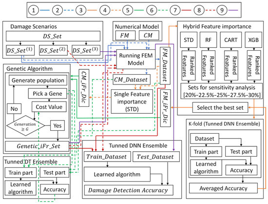
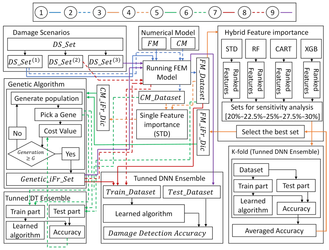
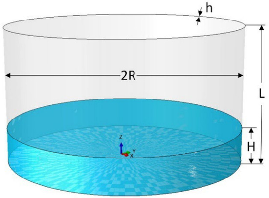
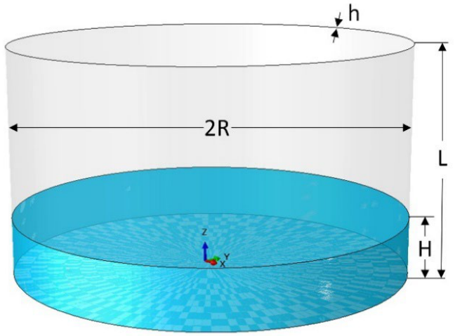
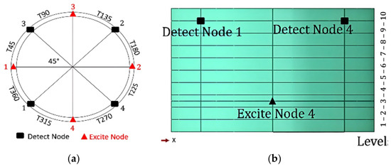
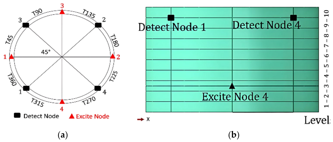
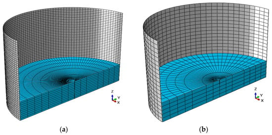
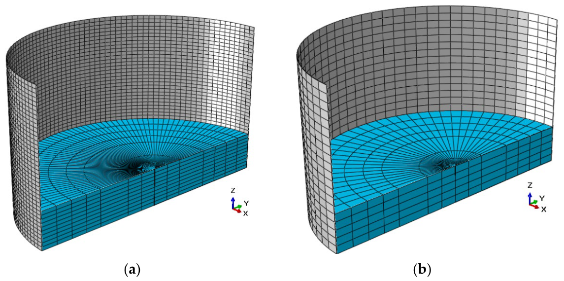
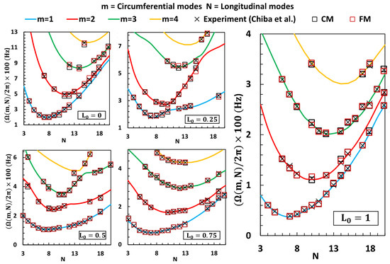
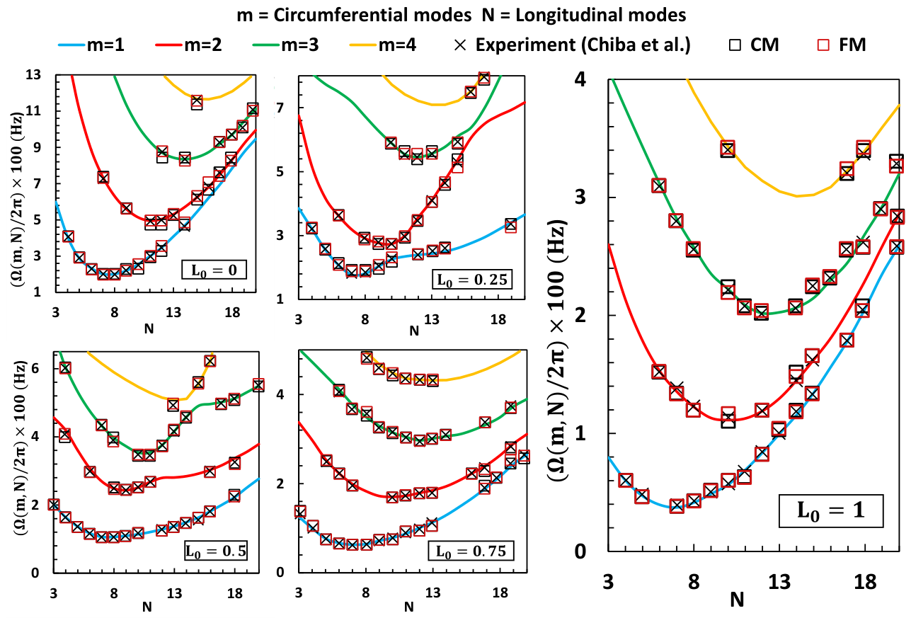
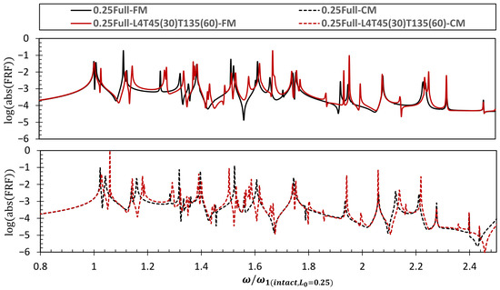
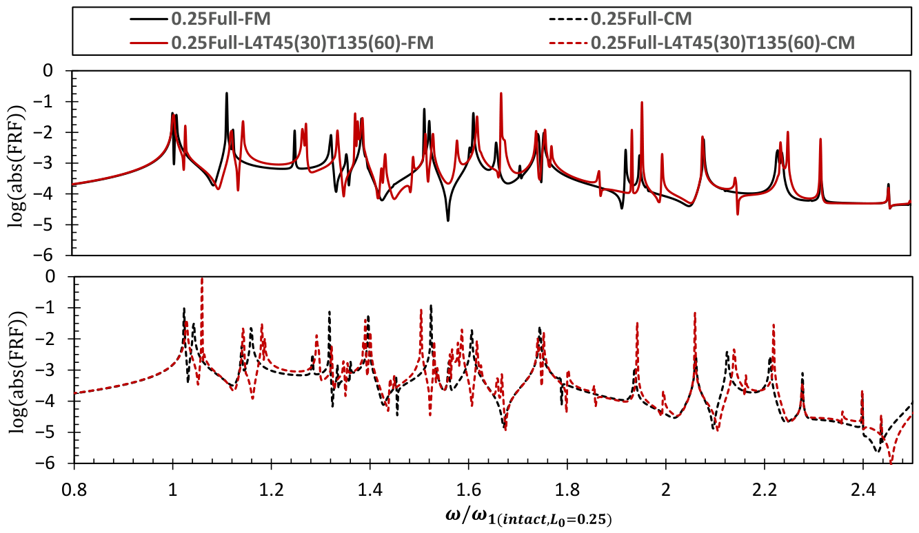
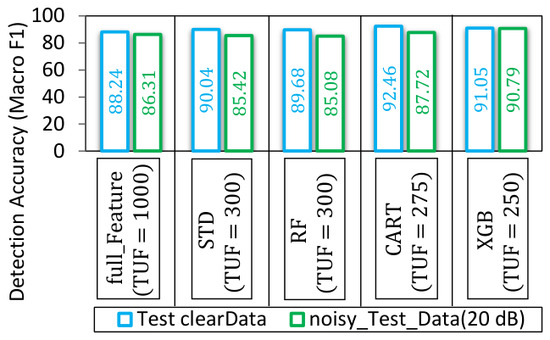
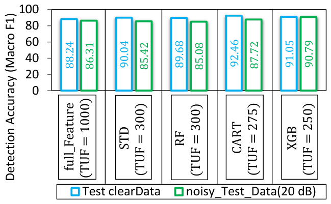
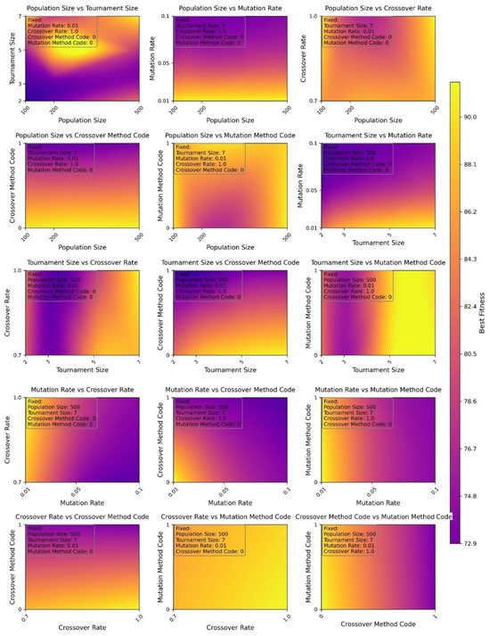
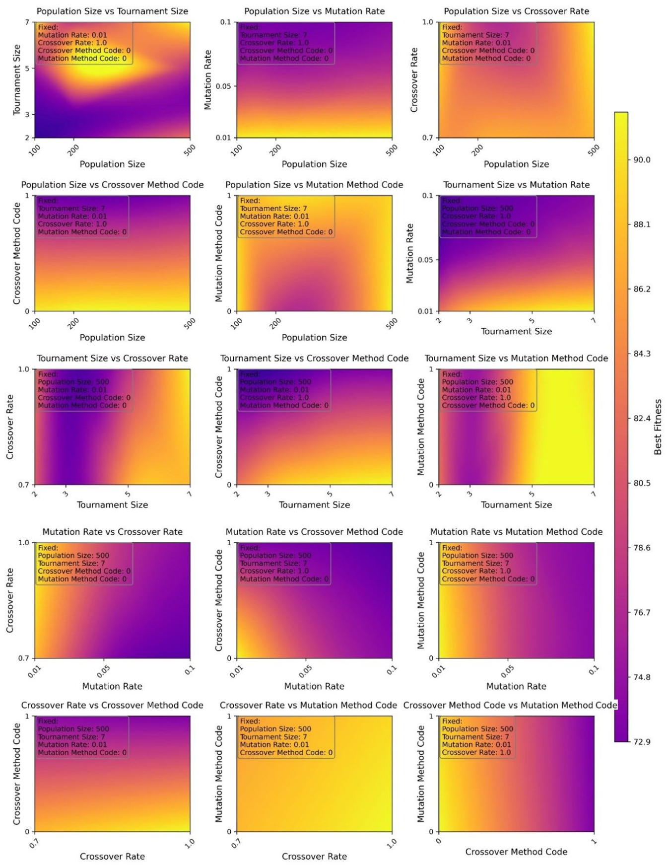
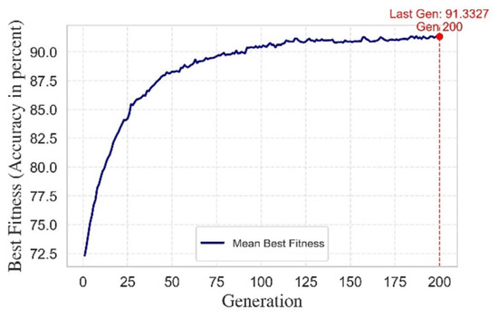
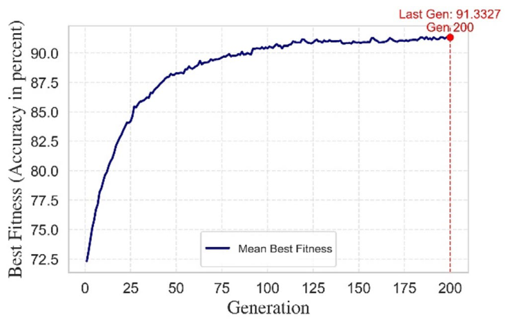
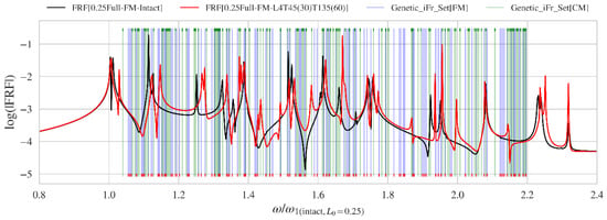
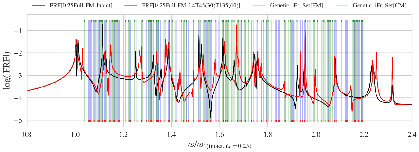
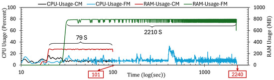
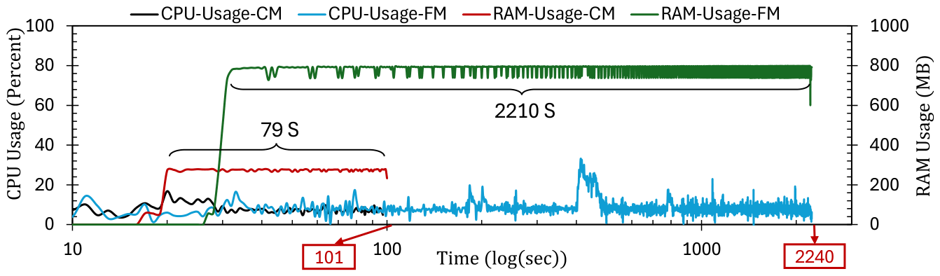
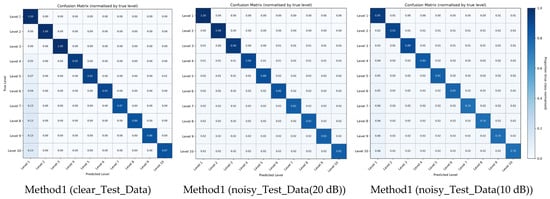
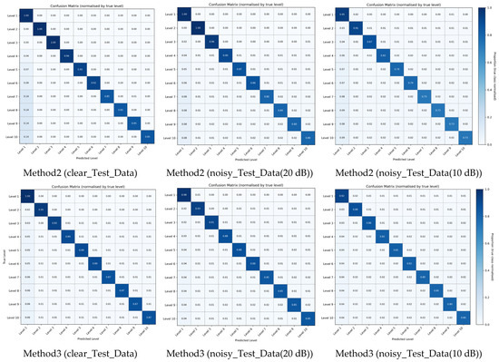
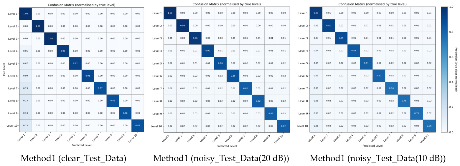
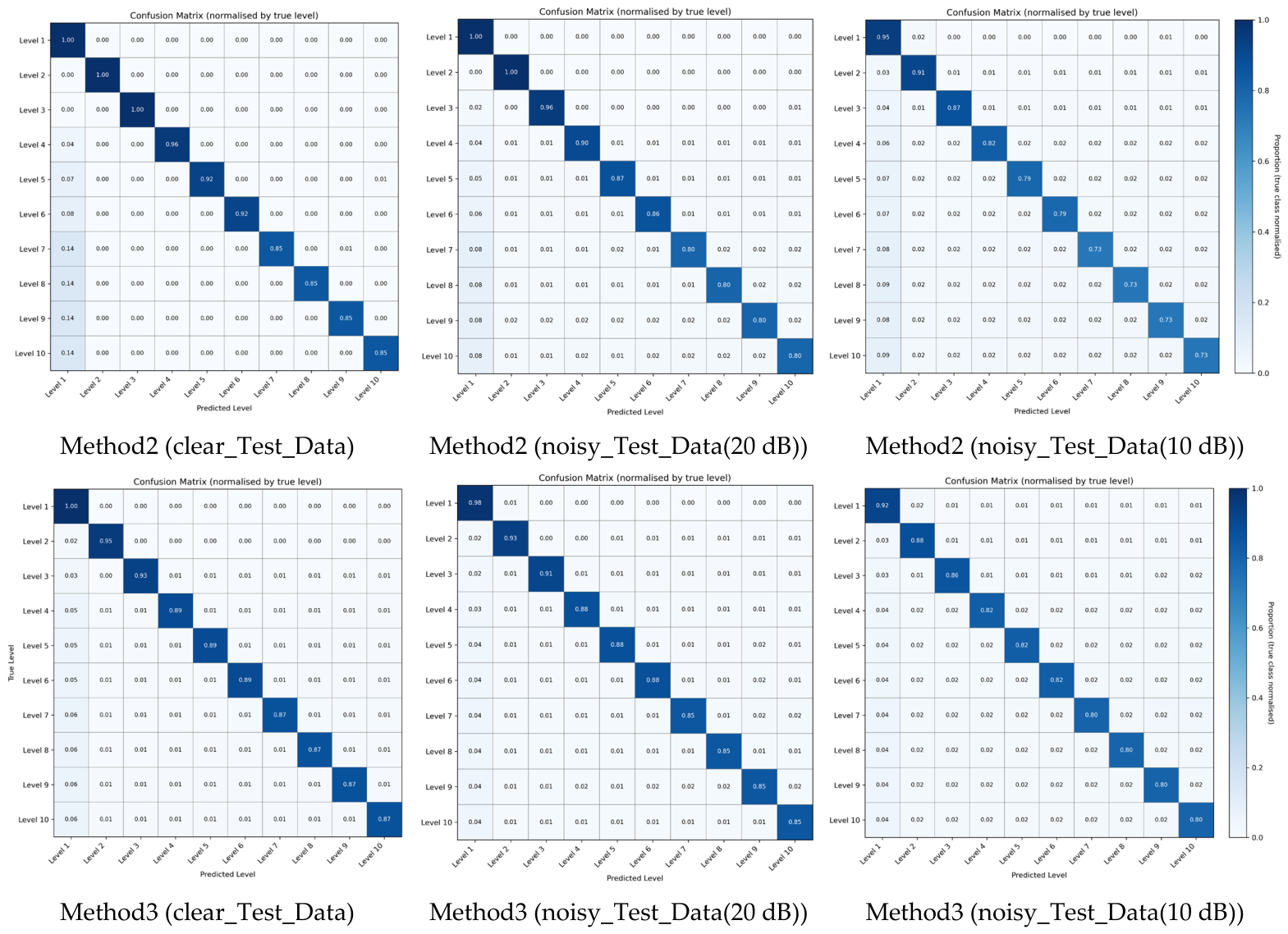
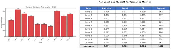
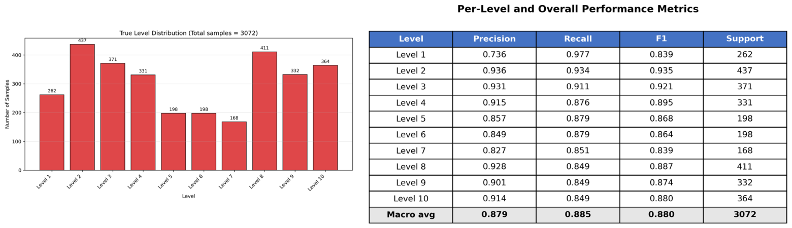
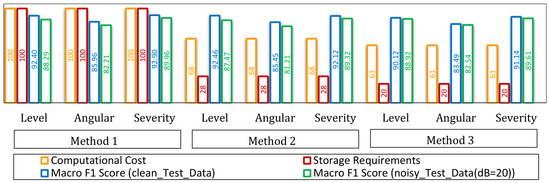
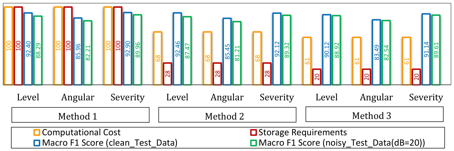

Disclaimer/Publisher’s Note: The statements, opinions and data contained in all publications are solely those of the individual author(s) and contributor(s) and not of MDPI and/or the editor(s). MDPI and/or the editor(s) disclaim responsibility for any injury to people or property resulting from any ideas, methods, instructions or products referred to in the content. |
© 2026 by the authors. Licensee MDPI, Basel, Switzerland. This article is an open access article distributed under the terms and conditions of the Creative Commons Attribution (CC BY) license.