


Abstract
Benzene is a carcinogenic urban volatile organic compound whose variability reflects interactions among emissions, atmospheric chemistry, and meteorology. We quantified relationships between hourly benzene concentrations and O3, CO, SO2, NO2, and more than twenty meteorological predictors using regulatory air-quality observations from the Ksaverska cesta urban background station in Zagreb, Croatia, complemented by NOAA GDAS meteorological data (2017–2023; n = 39,124). Metaheuristically optimized tree-ensemble models were interpreted using iterative Shapley Additive Global Importance (iSAGE), SHapley Additive exPlanations (SHAP), and an environmental settings framework. The novelty of the study lies in integrating global predictor importance, signed local SHAP attributions, and environmental-setting classification to interpret benzene variability within recurring emission–chemistry–meteorology regimes. The best-performing Extra Trees model achieved R2 = 0.87, RMSE = 0.46 µg m−3, and MAE = 0.24 µg m−3. iSAGE identified CO (1.47), O3 (0.55), and near-surface air temperature (0.35) as the leading predictors of modeled benzene concentrations, whereas SO2 (0.18) and NO2 (0.07) had substantially lower global importance. SHAP showed a positive CO-benzene association, with relative contributions shifting from negative to positive at approximately 0.3–0.6 mg m−3; O3 contributions became predominantly negative above 30–40 µg m−3; and temperature contributions shifted from positive below 7 °C to negative across 7–12 °C. Environmental setting analysis associated the strongest benzene accumulation with stable winter conditions and the weakest accumulation with well-ventilated, photochemically active regimes. These site- and model-specific results reveal nonlinear co-pollutant and meteorological influences on urban benzene variability. Theoretically, the study advances the interpretation of urban VOC variability by linking model-based predictor attributions with physically interpretable atmospheric regimes; practically, it supports the identification of conditions favoring benzene accumulation and can inform regime-sensitive air-quality assessment and management.
1. Introduction
Benzene is a ubiquitous urban volatile organic compound (VOC) and a well-recognized human carcinogen, for which adverse health effects have been documented even at low ambient concentrations [1]. In cities, it originates predominantly from vehicular exhaust, fuel evaporation, and other combustion-related activities. However, its ambient levels and temporal variability are not governed solely by emission strength but instead arise from a complex interplay between source activity, atmospheric mixing, photochemical transformation, and interactions with co-emitted pollutants. Urban atmospheric processes such as boundary-layer dynamics, photochemical oxidation, and co-pollutant interactions (e.g., with NOx and O3) create temporally and spatially heterogeneous exposure patterns [2,3], making robust characterization of benzene variability essential for effective urban air quality management [4].
From a physicochemical perspective, the relationships between benzene and the considered co-pollutants arise from a combination of common emission sources, atmospheric transformation, and meteorological modulation rather than from direct chemical interactions alone. Benzene and CO are commonly co-emitted during incomplete combustion, particularly from road traffic and residential heating, making CO a useful indicator of combustion-related benzene emissions. NO2 also reflects traffic and other combustion sources, while participating in VOC–NOx photochemical cycling that regulates tropospheric O3 formation. Benzene contributes to this chemistry as a reactive aromatic VOC, but its atmospheric degradation is initiated predominantly by OH radicals; consequently, O3 is interpreted primarily as an indicator of photochemical processing and the broader oxidative state of the atmosphere rather than as a direct sink for benzene. SO2 has no major direct chemical coupling with benzene under ambient urban conditions but may covary with it during combustion episodes and periods of restricted dispersion. Temperature exerts competing effects by influencing fuel and solvent evaporation, seasonal heating emissions, reaction kinetics, and boundary-layer development. The resulting relationships may therefore change in magnitude and direction across different emission, photochemical, and dispersion regimes [2,3,5,6,7].
Recent observational and modeling studies demonstrate that, despite substantial reductions in urban benzene concentrations in many regulated environments, pronounced spatial, seasonal, and source-related variability persists. A pan-European assessment of 22 monitoring sites in 19 cities during 2017–2022 identified benzene as the second most abundant BTEX compound and reported comparable median levels across urban-background, traffic, and industrial sites, with morning and evening enhancements associated with traffic, residential heating, and atmospheric stagnation [8]. A 30-year measurement record from the Zurich region documented an approximately 87% decrease in benzene concentrations between 1994 and 2024 following the implementation of VOC emission controls, while characteristic winter maxima remained evident [9]. High-time-resolution measurements in Marseille further distinguished traffic exhaust, fuel evaporation, industrial activity, shipping, urban background, and cold-season residential heating as contributing urban VOC source regimes [10]. At the global scale, ensemble machine learning combined with meteorological normalization confirmed that ambient benzene variability reflects the combined effects of emission changes and meteorological conditions [11]. These studies have substantially advanced the assessment of urban concentration trends, source contributions, and meteorological influences; however, comparatively limited attention has been given to how the global importance and signed local effects of individual co-pollutant and meteorological predictors change across recurring urban atmospheric regimes.
Conventional statistical and process-based modeling approaches often struggle to adequately resolve the nonlinear physicochemical processes, heterogeneous emission sources, and tightly coupled transport-chemistry interactions that govern secondary pollutant formation and shape the high-dimensional, dynamically evolving nature of urban atmospheric systems. In response to these limitations, artificial intelligence (AI) and machine learning (ML) techniques have gained increasing prominence in atmospheric sciences over the past decade, owing to their capacity to learn complex, multivariate relationships directly from observational data [12,13]. Data-driven methods such as random forests, gradient boosting algorithms, and neural networks have demonstrated strong predictive performance by capturing interactions among meteorological, chemical, and emission-related variables that are frequently oversimplified or neglected in traditional frameworks [14]. Despite these advances, most ML models remain inherently opaque, functioning as “black boxes” that offer limited insight into the underlying drivers of their predictions. This lack of transparency poses a critical barrier to their broader adoption for scientific interpretation, process understanding, and evidence-based policymaking.
Explainable artificial intelligence (XAI) has emerged as a promising approach to address this limitation. Methods such as SHapley Additive exPlanations (SHAP) and Shapley Additive Global Importance (SAGE) provide quantitative insights into the contributions of individual predictors and their interactions within complex models [15]. These approaches enable the identification of nonlinear dependencies and offer a pathway toward linking data-driven models with physical interpretation in urban atmospheric research.
Explainable ML methods are increasingly used to interpret complex atmospheric processes that are difficult to resolve using conventional statistical approaches. Recent studies have demonstrated that SHAP-based analyses can reveal physically meaningful insights into atmospheric chemistry and pollutant dynamics, including the identification of chemical drivers of fine particulate matter oxidative potential [16,17,18], the disentanglement of nonlinear precursor interactions governing O3 formation [5], and the elucidation of couplings between urban heat island effects and pollutant dynamics [19]. Methodological developments have further extended the use of SHAP toward more explicit representation of atmospheric chemistry. For example, Yao et al. (2025) proposed the SHAP Interaction Redistribution Analysis (SIRA) framework to better separate VOC photochemical losses from emission contributions during O3 formation across different atmospheric conditions [5].
At the same time, urban air pollution is increasingly recognized as a regime-dependent phenomenon in which pollutant concentrations emerge from interactions among emission intensity, atmospheric chemistry, and meteorological structure rather than from individual drivers acting independently. Although SHAP provides powerful tools for identifying nonlinear predictor–response relationships, interpretation at the level of individual variables does not directly reveal the atmospheric regimes under which these relationships operate. Translating SHAP-based explanations into coherent environmental contexts therefore remains an important challenge. One approach to address this limitation is to integrate SHAP interpretation with environmental settings (ES), which represent characteristic atmospheric regimes defined by coupled chemical and meteorological conditions [20,21]. Clustering SHAP contribution patterns into ES enables the identification of recurring atmospheric states, defined here as characteristic combinations of pollutant and meteorological conditions under which similar patterns of predictor contributions govern benzene variability, thereby linking ML explanations with physically interpretable atmospheric processes.
Against this background, the present study provides a predictor-centered extension of our previous setting-based analysis of benzene behavior in Zagreb [20]. Whereas Bešlić et al. [20] focused primarily on identifying and characterizing seven environmental settings (C0–C6) and determining which settings were associated with benzene extremes, the present study examines the global hierarchy and predictor-specific response patterns underlying those settings. The regional contribution lies in the use of a seven-year hourly regulatory monitoring dataset to characterize co-pollutant and meteorological associations with benzene at an urban background site in Zagreb. The broader methodological contribution is the integration of iSAGE-based global importance, absolute and relative SHAP impacts, and the environmental-settings framework, enabling dominant predictors to be distinguished from secondary contextual modifiers and their nonlinear responses to be interpreted within recurring emission–chemistry–meteorology regimes.
The study specifically addresses the following questions: (1) Which co-pollutant and meteorological variables provide the greatest predictive information for hourly benzene concentrations? (2) How do the direction and magnitude of the leading predictor contributions change across their observed ranges, including nonlinear transition regions? and (3) How do these relationships differ among pollution-enhancing, transitional, and pollution-suppressing environmental settings? To address these questions, metaheuristically optimized tree-ensemble models were applied to hourly observations from 2017–2023, with benzene defined as the target variable and O3, CO, SO2, NO2, and meteorological parameters treated as explanatory predictors. The results are interpreted as site- and model-specific associations and not as formal source apportionment or direct causal evidence.
2. Materials and Methods
2.1. Data Sources and Study Area
The analysis was conducted using multi-year air quality and meteorological data covering the 2017–2023 period for the city of Zagreb, Croatia. The City of Zagreb has a temperate humid continental climate, characterized by warm and occasionally hot summers and moderately cold winters with occasional snowfall. According to the 1991–2020 climatological normal for the Zagreb–Maksimir station, Zagreb has a temperate humid continental climate characterized by warm summers and moderately cold winters. Stable winter anticyclonic conditions are frequently accompanied by temperature inversions, which restrict vertical mixing and favor the accumulation of air pollutants within the near-surface atmospheric layer. The location of Zagreb and the Ksaverska cesta monitoring station is shown in Figure S1 of the Supplementary Materials.
The analysis was based on data from the Ksaverska cesta urban background air quality monitoring station (45°50′09″ N, 15°58′59″ E), located in a moderately populated urban-residential area influenced by local traffic emissions and residential heating. Measurements of benzene, NO2, CO, SO2, and O3 were performed within the municipal air quality monitoring network funded by the City of Zagreb. Hourly pollutant concentrations were obtained using standardized reference methods in accordance with EN 14211 (2012), EN 14212 (2012), EN 14626 (2012), EN 14625 (2012), and EN 14662-3 (2015) [22,23,24,25,26]. Measurement-level quality assurance and quality control were performed as part of the routine operation of the municipal monitoring network, in accordance with the applicable reference methods and regulatory monitoring procedures. These procedures included routine calibration and analyzer performance checks, scheduled instrument maintenance, and technical validation and quality flagging of hourly measurements. Only measurements classified as valid following the network-level QA/QC and validation process were considered for the present analysis.
To better capture the role of meteorology in shaping urban air quality, the in situ dataset was complemented with surface and upper-air meteorological variables retrieved from the NOAA GDAS1. GDAS provides three-hourly global meteorological fields based on the assimilation of observational and model-derived data, ensuring internally consistent atmospheric conditions across spatial and temporal scales. More than 20 meteorological and thermodynamic parameters were extracted, including temperature, pressure, humidity, wind characteristics, precipitation, and indicators of atmospheric stability and convective activity [27]. These variables were temporally aligned with air quality observations and enabled the interpretation of benzene variability within a coherent meteorological context relevant to urban atmospheric processes. Full names, units, and concise physical descriptions of all GDAS-derived meteorological variables, together with the abbreviations used throughout the manuscript, are provided in Tables S1 and S1a of the Supplementary Materials.
2.2. Data Processing and Preparation
Prior to dataset integration, the air-quality measurements underwent routine network-level QA/QC and technical validation in accordance with the applicable reference methods and regulatory monitoring procedures. Only measurements classified as valid following this process were retained for the analysis. The air-quality and meteorological datasets were subsequently processed using a Python-based pipeline. Timestamps were converted to a common time basis, ordered chronologically, and checked for duplicate records, missing timestamps, and inconsistencies in the temporal sequence. The three-hourly GDAS meteorological data were temporally aligned with the hourly air-quality observations using piecewise linear interpolation between consecutive GDAS records to obtain hourly values on a UTC time grid. Missing values were not imputed; observations lacking a valid value for any of the variables included in the analysis were excluded using complete-case filtering. Following these procedures, the final dataset comprised 39,124 complete and temporally aligned hourly observations. No additional concentration-based outlier removal was applied to measurements that had passed the network-level validation procedure. Benzene concentration was defined as the target variable, while co-pollutant concentrations and meteorological parameters were treated as explanatory predictors. Prior to model development, all variables were standardized to ensure numerical comparability across predictors and to reduce potential biases arising from differences in scale and physical units.
2.2.1. Modeling Framework
The modeling workflow comprised four sequential stages: (i) development and screening of candidate ensemble models, (ii) metaheuristic hyperparameter optimization, (iii) independent and temporal model validation, and (iv) explainable-AI interpretation and identification of environmental settings.
The modeling framework was designed to jointly address predictive accuracy and interpretability, with the objective of capturing nonlinear and interaction-driven relationships governing urban benzene variability. Analyses were conducted in Python 3.8.18 using a dedicated computational environment. The main packages used for data processing, modeling, optimization, and interpretation were NumPy (v1.24.4), pandas (v1.5.3), SciPy (v1.10.1), scikit-learn (v1.3.0) [28], together with LightGBM (v4.5.0) [29] and XGBoost (v2.1.1) [30]. Metaheuristic optimization was implemented using the Mealpy framework (v3.0.1), while model interpretation and post hoc analyses were performed using SHAP (v0.44.1) [31] and sage-importance (v0.0.5) [32]. Dimensionality reduction in SHAP contribution patterns was conducted using PaCMAP (v0.7.6) [33], followed by clustering with HDBSCAN (v0.8.33) [34] to identify ES. Additional statistical analyses and data consistency checks were performed in R (version 4.5.2) [35].
Several ensemble-based ML algorithms were evaluated, including Extra Trees [36], Gradient Boosting [37], its histogram-based implementation [28], LightGBM [29], and XGBoost [30]. These algorithms were selected because of their ability to capture nonlinear and multivariate dependencies commonly observed in atmospheric datasets. The complete dataset was first randomly divided into training (80%) and independent test (20%) subsets using random seed 42. Candidate model screening and hyperparameter optimization were performed exclusively within the training subset. The candidate models were initially evaluated using five-fold cross-validation, after which the three best-performing models, Extra Trees, LightGBM, and XGBoost, were refined using metaheuristic hyperparameter optimization based on Harris Hawks Optimization [38] and the Sine Cosine Algorithm [39]. Hyperparameters were optimized within bounded search spaces using mean cross-validated R2 as the objective function, with each optimization run comprising 10 epochs and a population size of 20. The best-performing Extra Trees configuration was subsequently refitted on the complete training subset and evaluated once on the untouched test subset using R2, root mean squared error (RMSE), and mean absolute error (MAE). In a separate sensitivity analysis, robustness to temporal dependence and potential temporal leakage was examined using five-fold forward-chaining validation implemented with TimeSeriesSplit in scikit-learn version 1.3.0. Random seed 42 was applied to the stochastic workflow components, including data partitioning, model initialization, cross-validation where applicable, and metaheuristic optimization. A schematic overview of the complete research workflow is provided in Figure S16 of the Supplementary Materials.
The decision to focus on tree-based ensemble models optimized using metaheuristic algorithms was motivated by both atmospheric and computational considerations. Urban benzene variability is governed by nonlinear and interaction-driven relationships among emissions, co-pollutants, atmospheric chemistry, and meteorology, which are unlikely to be fully captured by predefined linear or additive functional forms. Tree-based ensembles are well suited to such tabular environmental datasets because they can represent nonlinear responses and combined effects among multiple predictors, while remaining compatible with post hoc interpretation methods such as SHAP and SAGE. From a computational perspective, hyperparameter tuning of tree-based ensembles involves a mixed and potentially large search space containing discrete, continuous, and interacting parameters. Metaheuristic algorithms provide a derivative-free optimization strategy that balances exploration of the broader search space with exploitation of promising parameter regions while limiting the number of candidate configurations that must be evaluated. This approach is less exhaustive than grid search and more adaptively guided than simple random search. Alternative hyperparameter-tuning strategies, including random search, grid search, and Bayesian optimization, may also be used, with Bayesian optimization offering a particularly strong sample-efficient alternative for expensive objective functions. Alternative modeling approaches include multiple linear regression, generalized additive models, support vector or kernel-based models, neural networks, process-based atmospheric models, and hybrid physics–machine learning frameworks. In this study, the optimized tree-ensemble approach was selected as a suitable compromise between predictive accuracy, robustness for nonlinear tabular data, computational feasibility, and explainability.
2.2.2. Model Interpretation
Model interpretation was conducted using iterative Shapley Additive Global Importance (iSAGE) and SHAP, two complementary XAI techniques that quantify global feature importance and local predictor contributions to model predictions [31,32]. iSAGE was used to evaluate global predictor relevance by estimating the degradation in model performance following the removal of individual variables and their interactions, thereby providing robust estimates of overall feature importance. Local interpretability was assessed using SHAP, which decomposes each individual prediction into the model baseline and additive predictor-specific contributions. In the present study, absolute SHAP impacts represent the signed, non-normalized contributions of individual predictors expressed on the original scale of the target variable, i.e., benzene concentration in µg m−3. Positive absolute SHAP impacts indicate that a predictor increases the modeled benzene concentration relative to the model baseline, whereas negative values indicate a decrease. The term “absolute” is used here to distinguish impacts expressed on the original target scale from normalized relative impacts and does not denote the mathematical absolute value of SHAP. Relative SHAP impacts were obtained by normalizing each signed predictor contribution with respect to the total magnitude of the SHAP contributions for the same observation and expressing it as a percentage. They therefore indicate the proportional contribution of an individual predictor within a particular model prediction while retaining the direction of its influence. Relative SHAP impacts do not represent percentage changes in measured benzene concentration, explained variance, global predictor importance, or causal effects [40].
Interpretation focused primarily on SHAP dependence relationships describing how modeled benzene concentrations respond to variations in individual predictors across their observed ranges. To facilitate structured analysis, predictors were grouped according to their global importance derived from iSAGE into high-, intermediate-, and low-contribution variables. This stratification enabled systematic comparison of response patterns while preserving the continuous representation of atmospheric and meteorological influences.
To organize the high-dimensional explanation patterns in accordance with the ES concept, SHAP values were embedded into a lower-dimensional space using PaCMAP [33] and clustered using the density-based HDBSCAN algorithm [34]. The resulting clusters were interpreted as ES, representing recurring atmospheric regimes defined by characteristic combinations of chemical and meteorological conditions influencing benzene variability. Cluster-level statistics, including frequency of occurrence and mean SHAP contributions, were evaluated to quantify the prevalence and influence of individual settings. At the variable level, characteristic predictor values within each ES were examined together with their associated SHAP contributions to link atmospheric conditions with modeled benzene responses. Throughout the Results and Discussion, the term “atmospheric states” refers to these ES-defined regimes (C0–C6). Each state represents a recurring multivariate emission–chemistry–meteorology context within which predictor-specific SHAP impacts are interpreted.
SHAP uncertainty and robustness considerations: SHAP values were interpreted as model-conditional attribution estimates for the final optimized Extra Trees model rather than as formal probabilistic uncertainty intervals. For a fixed trained model and background dataset, SHAP attributions are deterministic. However, attribution patterns may vary with data sampling, train and test partitioning, and stochastic elements of model fitting. In this study, robustness was addressed at the modeling level through fixed random initialization, five-fold cross-validation for candidate model screening and hyperparameter optimization, independent 80/20 train-test evaluation, and additional forward-chaining time-series validation. The interpretation therefore focused on broad, high-density, physically coherent SHAP response patterns, particularly for the dominant predictors identified by iSAGE, rather than on isolated observations or exact numerical breakpoints. Consequently, the transition ranges discussed in the SHAP dependence plots should be regarded as approximate model-conditional response regions rather than formal statistical thresholds. Formal uncertainty quantification based on bootstrap resampling or ensemble SHAP distributions was not performed and is identified as an important direction for future work.
Computational costs were recorded for the final benzene-regression workflow. The analysis was executed on a Microsoft Windows Server 2022 Standard workstation with two Intel Xeon Gold 5418Y processors, 48 physical cores/96 logical processors in total, and 128 GB RAM. The full workflow required 124,621.53 s. The iSAGE calculation required 3513.03 s, the SHAP value calculation required 209.85 s, SHAP interaction analysis required 5731.87 s, SHAP clustering required 65.01s, and SAGE calculation required 4164.67 s. The total runtime of the SHAP-related stages was 6006.73 s, while the combined runtime of SAGE and iSAGE was 7677.71 s. All reported runtimes correspond to CPU-based execution.
3. Results
3.1. Temporal Variability, Descriptive Statistics, and Model Performance
Long-term air quality conditions in Zagreb during the 2017–2023 period were analyzed using 39,124 hourly observations to establish the environmental context for the subsequent explainable AI analysis of benzene variability. All descriptive values reported below were calculated from the final QA/QC-filtered analytical dataset, while the underlying monitoring dataset and its earlier descriptive characterization were reported by Bešlić et al. (2026) [20]. Summary statistics for benzene and the measured co-pollutants are presented in Table 1, whereas complete descriptive statistics for all model inputs are provided in Table S1.
Table 1.
Descriptive statistics of measured pollutant concentrations in the final analytical dataset (2017–2023; n = 39,124 hourly observations). The underlying monitoring dataset was previously described by Bešlić et al. (2026) [20].
To provide a direct visual overview of benzene variability, Figure 1 presents daily mean concentrations and their 30-day moving average during 2017–2023. The time series shows pronounced seasonal variability, with recurrent winter maxima and lower warm-season concentrations, as well as a non-monotonic interannual pattern. Mean benzene concentration over the study period was 1.02 µg m−3, with episodic peaks reaching 13.52 µg m−3. The annual mean decreased from 1.50 µg m−3 in 2018 to 0.63 µg m−3 in 2022, followed by an increase to 1.04 µg m−3 in 2023, indicating a non-monotonic temporal evolution [20]. Co-pollutant trends exhibited broadly similar patterns. Mean annual NO2 concentrations decreased from 18.7 to 14.3 µg m−3, while CO decreased from 0.36 to 0.28 mg m−3 [20], consistent with reductions in traffic-related and other combustion emissions, including the influence of pandemic-related mobility restrictions [41]. SO2 concentrations remained generally low, whereas O3 exhibited the greatest overall variability and recurrent summer exceedances of the eight-hour threshold of 120 µg m−3 [20].
Figure 1.
Temporal variation in benzene concentrations at the Ksaverska cesta urban background station during 2017–2023. The thin line represents daily mean concentrations calculated for days with at least 18 valid hourly observations (≥75% daily data completeness), whereas the thick line represents the centered 30-day moving average. Gaps indicate periods that did not meet the daily completeness criterion. Daily aggregation was applied solely for visualization; all modeling analyses were conducted using the QA/QC-filtered hourly dataset.
At broader spatial scales, previous assessments report limited continental differentiation in urban benzene concentrations, highlighting the dominance of diffuse urban sources such as traffic and distributed combustion over large point emitters, particularly in cities without significant oil and gas activities [42,43]. However, within individual urban environments, benzene variability remains strongly modulated by interactions among co-pollutants, meteorological conditions, and seasonal dynamics, which are still insufficiently quantified.
These findings underscore that urban benzene concentrations are governed by coupled emission–chemistry–meteorology processes rather than by single drivers acting independently. The relative importance of these factors and their nonlinear interactions are difficult to resolve using conventional statistical approaches. To address this challenge, this study employs an explainable artificial intelligence framework that integrates machine learning with SHAP-based interpretation, enabling a quantitative assessment of predictor contributions and their role within distinct urban atmospheric settings.
Prior to interpretation, the predictive performance of the final model was evaluated using standard goodness-of-fit metrics. The Extra Trees model achieved R2 = 0.87, RMSE = 0.46 µg m−3, and MAE = 0.24 µg m−3. The observed and predicted concentration distributions showed broad agreement across the training and test subsets (Figure S2).
3.2. Global Hierarchy of Co-Pollutant and Meteorological Predictors
Global predictor importance derived from iSAGE revealed a strongly differentiated hierarchy of chemical and meteorological predictors associated with modeled benzene variability at the study site (Figure 2; complete numerical values are provided in Table S2). CO was the dominant predictor (iSAGE = 1.47), followed by O3 (0.55) and near-surface air temperature, t02m (0.35). The CO score was approximately 2.7 times higher than that of O3 and more than four times higher than that of t02m, indicating the predominance of the combustion-related signal in the fitted model.
Figure 2.
Global predictor importance for modeled hourly benzene concentrations estimated using iSAGE. Predictors are ranked according to their final iSAGE importance scores. Positive scores indicate a deterioration in model performance following predictor removal, whereas negative scores indicate limited or redundant incremental predictive information within the fitted predictor set and do not represent negative physical effects. Exact numerical values are provided in Table S2, while the extended original visualization is retained as Figure S3 in the Supplementary Materials.
The next-ranked variables, momentum flux intensity (mofi; 0.20), SO2 (0.18), and surface temperature (tmps; 0.16), showed substantially lower importance. All remaining predictors had positive scores below 0.12, including NO2 (0.07), planetary boundary-layer height (pblh; 0.04), and relative humidity (rh2m; 0.04). These lower-ranked variables are therefore interpreted as secondary contextual modifiers rather than predictors exerting influence comparable to CO, O3, or t02m. Negative iSAGE values indicate limited incremental predictive information within the fitted predictor set and should not be interpreted as negative physical effects. Accordingly, the detailed SHAP discussion focuses primarily on CO, O3, and t02m, while secondary variables are used to refine the interpretation of individual environmental settings.
Importantly, the global importance of SO2 and particularly NO2 was substantially lower than that of the dominant co-pollutant predictors. Relative to CO, the iSAGE scores of SO2 and NO2 were approximately 13% and 4.5%, respectively; relative to O3, they were approximately 34% and 12%, respectively. These ratios compare the magnitudes of the iSAGE scores and do not represent proportions of explained variance. Thus, although their local SHAP patterns may remain informative under specific environmental settings, SO2 and NO2 are interpreted here as secondary contextual indicators rather than as primary controls of benzene variability. Several predictors exhibit negative iSAGE values, indicating that their removal does not degrade model performance and suggesting that these variables provided limited additional information beyond higher-ranking variables.
Given the hierarchy of predictors revealed by the iSAGE analysis, the subsequent SHAP interpretation focuses on the variables with the strongest explanatory power. CO, O3, and near-surface air temperature represent three key domains, emissions, atmospheric chemistry, and meteorological control, that jointly govern benzene variability. The following section therefore examines these relationships in detail to identify nonlinear responses, threshold behavior, and regime-dependent interactions across the ES defined by Bešlić et al. (2026) [20].
3.3. SHAP Response Patterns of CO, O3, and Near-Surface Temperature
Throughout the following analysis, absolute SHAP impacts are used to assess the direction and magnitude of predictor contributions in concentration units, whereas relative SHAP impacts indicate their proportional contribution within individual model predictions. The SHAP analysis confirms the dominant role of three predictors in governing benzene variability: CO, O3, and near-surface air temperature (t02m). Together, these variables capture the interplay between combustion-related emissions, atmospheric oxidative processes, and seasonal meteorological conditions. CO primarily reflects the influence of direct emission sources, O3 represents the oxidative state of the atmosphere, and temperature regulates boundary-layer development and atmospheric mixing. Taken together, their SHAP responses provide a process-oriented interpretation of benzene dynamics in the studied urban environment. The SHAP-derived transition ranges discussed below are therefore interpreted as approximate model-conditional response regions, not as formal statistical thresholds with confidence intervals.
3.3.1. CO—Emission-Driven Influence
The SHAP response to CO reveals a strong and nearly linear positive association with benzene in terms of absolute impacts (Figure 3a), with contributions occasionally exceeding 4–5 µg m−3 at elevated concentrations. This behavior reflects the shared combustion-related origin of CO and benzene, primarily associated with vehicular exhaust and residential heating emissions [3]. As CO concentrations increase, the model assigns progressively larger absolute contributions to benzene variability, underscoring the dominant role of combustion-related sources.
Figure 3.
SHAP impacts of CO on modeled benzene concentrations: (a) absolute SHAP impacts; (b) relative SHAP impacts; and (c) combined representation of absolute and relative SHAP impacts. Absolute impacts denote signed contributions on the original target scale and are expressed in µg m−3, whereas relative impacts represent signed percentages of the total local SHAP attribution magnitude. Points represent individual observations, and grey shading indicates the environmental settings (C0–C6) defined in Bešlić et al. (2026) [20].
In contrast, the relative SHAP patterns exhibit a pronounced nonlinear, threshold-like response (Figure 3b). At low CO concentrations (<0.3 mg m−3), which dominate much of the dataset, relative contributions are predominantly negative (−20% to −60%). These conditions correspond to well-mixed boundary layers and low co-emission intensity, under which combustion sources exert only limited control over benzene variability. A rapid transition toward positive relative contributions occurs within the intermediate CO range of approximately 0.3–0.6 mg m−3, marking a shift from dilution-controlled to emission-dominated conditions. This transition is likely to reflect periods of intensified traffic or combustion activity combined with reduced atmospheric ventilation.
At higher CO concentrations, relative SHAP contributions stabilize at approximately 40–60%, indicating saturation-like behavior in which further increases in CO provide diminishing additional explanatory power. The combined distribution of absolute and relative SHAP impacts (Figure 3c) further shows that both the magnitude and proportional influence of CO vary systematically across ES-defined atmospheric states (C0–C6). Under clean and well-mixed conditions, characterized by negative relative SHAP contributions, absolute impacts remain close to zero, indicating a limited role of CO in explaining benzene variability. As relative contributions become positive (approximately 20–60%), absolute SHAP values increase sharply, reaching up to 5 µg m−3 and indicating emission-driven conditions in which elevated CO and benzene concentrations co-occur because of common combustion sources.
Across the ES defined by Bešlić et al. (2026) [20], the CO–benzene relationship is strongly modulated by atmospheric regime. The largest positive SHAP impacts occur in the pollution-enhancing settings C6 and C4, where combustion emissions accumulate under shallow boundary layers and weak ventilation. In contrast, the well-ventilated settings C0, C1, and C3 exhibit weak or negative responses, reflecting efficient dilution and photochemical processing that limit benzene accumulation (Figure S4, Supplementary Materials). Transitional settings (C2 and C5) display intermediate responses, indicating mixed atmospheric states in which moderate combustion influence coexists with meteorological conditions that only partly restrict dispersion. In C2, the influence of CO remains relatively weak and decoupled from benzene variability, whereas C5 represents a late-winter transition in which moderate emissions may still contribute to short-term benzene persistence under relatively stable anticyclonic conditions.
3.3.2. O3—Oxidative Influence
The joint distribution of absolute and relative SHAP impacts for O3 (Figure 4c) highlights its distinct role compared with emission-related predictors and confirms it as the second most influential variable governing benzene variability. Unlike CO, which directly traces combustion emissions, O3 exhibits a predominantly inverse association with benzene, reflecting its role as an indicator of atmospheric oxidative capacity and photochemical activity rather than a direct emission proxy. As O3 concentrations increase beyond approximately 30–40 µg m−3, SHAP impacts progressively shift toward negative values, consistent with photochemically active conditions in which OH-mediated benzene oxidation, together with changes in atmospheric ventilation, reduces benzene persistence. O3 is therefore interpreted as a proxy for the broader oxidative and photochemical state of the atmosphere rather than as the principal direct oxidant of benzene.
Figure 4.
SHAP impacts of O3 on modeled benzene concentrations: (a) absolute SHAP impacts; (b) relative SHAP impacts; and (c) combined representation of absolute and relative SHAP impacts. Absolute impacts denote signed contributions on the original target scale and are expressed in µg m−3, whereas relative impacts represent signed percentages of the total local SHAP attribution magnitude. Points represent individual observations, and grey shading indicates the environmental settings (C0–C6) defined in Bešlić et al. (2026) [20].
At very low O3 concentrations (<20 µg m−3), both relative SHAP contributions and absolute impacts become positive and reach their maximum values, with relative contributions exceeding approximately 10% and absolute impacts approaching 0.5 µg m−3 (Figure 4a,b). These conditions are characteristic of winter stagnation environments in which photochemical activity is suppressed and atmospheric mixing is limited. Although O3 and benzene do not share emission sources, their apparent positive association reflects the co-occurrence of broader atmospheric processes, such as reduced dispersion, enhanced thermal stability, and pollutant accumulation, rather than a direct causal relationship between the two species [21]. This pattern corresponds most closely to the winter inversion–stagnation regime C6, where benzene variability is dominated by combustion-related pollutants while O3 plays only a secondary role [20].
As O3 concentrations increase beyond approximately 30–40 µg m−3, SHAP impacts progressively shift toward negative values, typically between −5% and −15%. This pattern is consistent with photochemically active conditions in which OH-mediated benzene oxidation, together with enhanced atmospheric ventilation, reduces benzene persistence [5]. The transition indicates a shift from emission-dominated stagnation toward a more photochemically active and better-ventilated atmospheric regime. Such behavior relates primarily to the pollution-suppressing regimes C0, C1, and C3, where stronger photochemical activity and deeper boundary layers promote both dilution and chemical degradation of benzene [20].
Cluster-resolved SHAP plots reveal subtle but meaningful differences among these regimes (Figure S5, Supplementary Materials). C1 shows the most consistently negative response, reflecting a clean and well-ventilated photochemical background. C0 exhibits slightly greater dispersion and occasional positive excursions at higher O3 levels, suggesting episodic transport or residual emission influence. By contrast, C3 maintains a stable negative trend typical of summer oxidation–ventilation conditions.
Intermediate O3 concentrations correspond to transitional atmospheric states in which residual emission signals coexist with progressively stronger oxidative removal. These conditions are best represented by the transitional regimes C2 and C5, where SHAP plots show moderate negative trends accompanied by greater dispersion of SHAP values. The two regimes nevertheless differ in structure. In C2, SHAP responses display greater variability and occasional positive excursions, suggesting that diffuse combustion inputs can intermittently reinforce benzene variability despite moderate O3 levels. In contrast, C5 exhibits a more consistently negative SHAP response across the intermediate O3 range, consistent with photochemically active conditions in which OH-mediated benzene oxidation and enhanced atmospheric ventilation reduce benzene persistence. This behavior reflects a transition toward stronger photochemical activity and more efficient atmospheric mixing as seasonal conditions evolve.
3.3.3. Temperature—Meteorological Influence
Air temperature (t02m) is a key meteorological regulator of benzene variability, influencing boundary-layer stability, emission intensity, and chemical removal processes. The joint distribution of absolute and relative SHAP impacts (Figure 5c) reveals a predominantly inverse relationship between temperature and benzene concentrations, indicating that higher temperatures generally correspond to lower benzene levels because of enhanced atmospheric mixing and photochemical degradation.
Figure 5.
SHAP impacts of near-surface air temperature on modeled benzene concentrations: (a) absolute SHAP impacts; (b) relative SHAP impacts; and (c) combined representation of absolute and relative SHAP impacts. Absolute impacts denote signed contributions on the original target scale and are expressed in µg m−3, whereas relative impacts represent signed percentages of the total local SHAP attribution magnitude. Points represent individual observations, and grey shading indicates the environmental settings (C0–C6) defined in Bešlić et al. (2026) [20].
At low temperatures (<7 °C), both relative and absolute SHAP values become positive (Figure 5a,b), indicating enhanced benzene accumulation under cold-season conditions. These situations are characterized by increased combustion emissions from residential heating together with suppressed vertical mixing associated with shallow boundary layers and frequent temperature inversions. Such conditions correspond predominantly to the winter stagnation regime C6 and, to a lesser extent, the transitional regime C5 [20]. In C6, cluster-specific SHAP patterns show the strongest positive impacts of temperature, reflecting the tight coupling between benzene and combustion emissions during stagnant winter conditions (Figure S6). Shallow boundary layers and weak ventilation allow pollutants to accumulate near the surface, producing the highest benzene concentrations observed in the dataset. By contrast, C5 represents a late-winter-to-early-spring transitional regime in which dispersion gradually improves and temperature-driven boundary-layer evolution becomes a primary modulator of benzene variability.
A rapid transition of SHAP impacts from positive to negative occurs between approximately 7 and 12 °C (Figure 5a,b), marking a threshold at which atmospheric dispersion and photochemical processes begin to dominate over emission-driven accumulation. At higher temperatures (>15 °C), SHAP impacts stabilize at modest negative values (relative impacts between −10% and −30%) with very low absolute contributions, indicating that further warming has limited additional influence once turbulent mixing and chemical removal processes prevail.
Cluster-resolved SHAP plots show that these warmer conditions correspond primarily to the pollution-suppressing regimes C0, C1, and C3, as well as the transitional regime C2 and the moderately pollution-enhancing regime C4 (Figure S6, Supplementary Materials). These regimes are generally associated with warm-season atmospheric states characterized by deeper boundary layers, stronger vertical mixing, and higher oxidative capacity, all of which limit benzene accumulation. Subtle inter-regime differences nevertheless remain evident. C1 exhibits the most stable negative response, reflecting well-ventilated photochemical conditions. C0 shows slightly greater dispersion of SHAP values, suggesting episodic transport or residual emission influence. C3 maintains a consistently negative trend typical of summer oxidation–ventilation conditions. In contrast, C4 displays a broader spread of impacts within moderate temperature ranges, consistent with enhanced anthropogenic activity combined with relatively shallow mixing layers.
The joint behavior of absolute and relative SHAP values further supports the consistency of the temperature effect: stronger proportional impacts coincide with larger absolute contributions, although both remain moderate in magnitude. Occasionally positive SHAP values at intermediate temperatures likely reflect short-lived atmospheric states, such as transient inversions, abrupt boundary-layer transitions, or coincident emission peaks, in which temperature temporarily reinforces pollutant accumulation.
3.4. Secondary Chemical Indicators and Meteorological Modifiers
Consistent with their comparatively low global iSAGE importance, NO2 and SO2 are considered here as secondary pollutant indicators. Their SHAP patterns are examined to refine the emission and dispersion context of individual environmental settings, rather than to imply an influence comparable to that of the dominant predictors CO and O3 or an independent causal control over benzene variability. The NO2 SHAP response exhibited a moderately nonlinear pattern (Figure S7a), reflecting the combined influence of emission intensity, atmospheric dispersion, and VOC–NOx photochemical interactions. At low concentrations (<10 µg m−3), SHAP impacts were consistently negative, indicating well-ventilated conditions in which benzene variability is governed primarily by atmospheric dilution. As NO2 increased to intermediate levels (approximately 10–25 µg m−3), SHAP responses approached neutral values, suggesting transitional atmospheric states where NO2 acts mainly as an indicator of combustion activity rather than a direct driver of benzene variability. At higher concentrations above 20–40 µg m−3, SHAP impacts became positive, consistent with emission-dominated conditions in which co-emitted pollutants accumulate under reduced dispersion. Beyond this range, the response flattened, indicating that once strong emission influence is established, further increases in NO2 provide limited additional explanatory power.
SO2, despite having a higher global importance than NO2, also behaved primarily as a secondary indicator of combustion-related conditions rather than as an independent chemical driver of benzene variability (Figure S9a,b). Under very low SO2 concentrations, SHAP impacts remained close to zero or slightly negative, consistent with well-ventilated conditions where combustion influence is weak, and benzene levels are controlled mainly by atmospheric dilution. As SO2 increased to moderate levels (≈0.7–1.5 µg m−3), SHAP responses became positive, reflecting episodes of co-emission and pollutant accumulation under more stable atmospheric conditions. At higher concentrations, impacts tended to level off, suggesting that once emission influence is established, benzene variability becomes increasingly governed by meteorological controls rather than further increases in SO2. Both NO2 and SO2 therefore act primarily as markers of combustion-influenced regimes (C4 and C6) relative to dispersion-dominated conditions (C0–C3) (Figures S8 and S10, Supplementary Materials). Accordingly, the NO2 and SO2 patterns do not alter the global predictor hierarchy identified by iSAGE; instead, they provide additional contextual resolution for distinguishing combustion-influenced, transitional, and dispersion-dominated environmental settings.
Several additional meteorological variables further refine the interpretation of benzene variability by highlighting the role of atmospheric stability and vertical mixing. Planetary boundary-layer height showed a clear inverse relationship with benzene concentrations (Figure S11a,b), emphasizing the central importance of vertical mixing in regulating pollutant accumulation. Shallow boundary layers (<200 m) were associated with positive SHAP impacts, reflecting strong vertical confinement and enhanced near-surface accumulation of emissions. As pblh increased to several hundred meters, SHAP impacts approached zero or became slightly negative, indicating progressive dilution under stronger turbulent mixing. At large pblh values (>1500 m), impacts clustered near zero, suggesting that once the boundary layer becomes sufficiently deep, additional increases in mixing depth exert little further influence on benzene variability.
Atmospheric stability indicators showed consistent behavior. The lifted index highlighted the influence of stability on pollutant confinement (Figure S13a,b): under unstable conditions (negative lisd), SHAP impacts were close to zero or negative, reflecting efficient vertical mixing, whereas increasingly stable conditions (approximately 5–10) produced progressively positive responses as pollutants became confined within the lower atmosphere. Relative humidity exerted a weaker but systematic influence (Figure S15a,b), acting mainly as an indicator of boundary-layer development. Across low to moderate humidity levels (≈20–70%), SHAP impacts remained close to zero, indicating that benzene variability is governed primarily by emissions and mixing processes. At higher humidity (>80%), impacts became slightly negative, consistent with atmospheric conditions that favor enhanced dispersion or dilution. Across ES [20], shallow boundary layers and moist stable conditions characterize confinement-dominated regimes (C4 and C6), whereas deeper mixing and drier conditions are typical of well-ventilated regimes (C0 and C3), with transitional responses observed in intermediate states (C2–C5) (Figures S12 and S14, Supplementary Materials).
Taken together, these results indicate that benzene variability at the study site reflects the combined influence of emission intensity, photochemical and oxidative atmospheric conditions, and boundary-layer dynamics, with the strongest accumulation occurring under stable winter conditions and the most efficient dilution during well-ventilated photochemical regimes. Overall, the results support a three-tier interpretation: CO represents the dominant combustion-related predictor, O3 and near-surface temperature provide the principal photochemical and meteorological modulation, and the remaining chemical and meteorological variables primarily refine the characterization of individual environmental settings. This hierarchy is specific to the studied site and model and should not be interpreted as a universal ranking of urban benzene sources or atmospheric processes.
4. Discussion
4.1. Interpretation of the Principal Findings in Relation to Previous Studies
The present results identify a strongly differentiated hierarchy of co-pollutant and meteorological predictors associated with hourly benzene variability at the Zagreb urban background site. The dominant importance of CO supports the interpretation that combustion-related activity represents the principal emission signal captured by the fitted model. This finding is consistent with recent European observations showing that urban benzene variability reflects mixed contributions from road traffic, residential heating, and atmospheric stagnation, as well as with high-time-resolution source-apportionment results from Marseille identifying traffic exhaust, fuel evaporation, and cold-season residential heating as important urban VOC sources [8,9,10,11]. The present analysis does not quantify source-specific contributions and should therefore not be interpreted as formal source apportionment. Rather, it indicates that the combustion-related information represented by CO provides substantially greater predictive information for benzene than the other measured co-pollutants.
The concentration-scale and relative SHAP responses further show that the importance of the combustion-related signal depends on atmospheric conditions. The transition toward positive CO impacts at approximately 0.3–0.6 mg m−3 reflects a shift from conditions in which combustion emissions have a limited local contribution to conditions characterized by stronger emission accumulation. The strongest positive impacts occurred within stable cold-season environmental settings, consistent with the recurrent winter maxima reported in long-term European benzene observations. The persistence of winter maxima even in urban areas where annual benzene concentrations have declined substantially emphasizes that emission controls and seasonal atmospheric confinement represent distinct determinants of short- and long-term variability [8,9].
O3 and near-surface temperature formed a second level of the predictor hierarchy. Their predominantly negative SHAP contributions under warmer and more photochemically active conditions are consistent with the joint influence of enhanced boundary-layer mixing, seasonal changes in combustion activity, and increased atmospheric processing. O3 is interpreted here as an indicator of the broader photochemical and oxidative atmospheric regime rather than as the principal direct oxidant of benzene. Accordingly, the transition toward negative O3 impacts above approximately 30–40 µg m−3 and the temperature transition across approximately 7–12 °C should be regarded as site- and model-specific response regions rather than universal atmospheric thresholds. Previous modeling studies similarly demonstrate that ambient benzene variability cannot be attributed to emission changes alone and requires simultaneous consideration of meteorological conditions and atmospheric transport [11].
SO2 and particularly NO2 showed substantially lower global importance than CO and O3. Their SHAP patterns nevertheless provide contextual information for distinguishing combustion-influenced, transitional, and dispersion-dominated settings. These variables should therefore be interpreted as secondary proxies for particular emission and chemical environments, rather than as major independent determinants of benzene variability. Planetary boundary-layer height, atmospheric stability, and relative humidity likewise refine the characterization of individual regimes by indicating the degree of vertical confinement and ventilation. Together, the results support a three-tier interpretation in which CO represents the dominant combustion-related predictor, O3 and near-surface temperature represent the principal photochemical and meteorological modulators, and the remaining variables provide secondary contextual resolution.
4.2. Methodological Contribution of the XAI-ES Framework
The methodological contribution of the present study lies not in identifying traffic, heating, or atmospheric stagnation as previously unknown influences on benzene, but in resolving how their model-based signatures vary across recurring atmospheric regimes. iSAGE provides a global hierarchy of predictor relevance, whereas absolute and relative SHAP impacts quantify the direction, magnitude, and proportional contribution of individual predictors within hourly model estimates. The environmental-settings framework subsequently places these local attributions within recurring emission–chemistry–meteorology contexts. This integration therefore extends conventional concentration-trend and source-oriented analyses by distinguishing globally dominant predictors from variables that become informative only under particular atmospheric states.
The present study also extends the previous setting-based analysis of the same monitoring dataset [20]. Whereas the earlier work primarily identified and characterized the environmental settings associated with benzene extremes, the current analysis focuses on the predictor hierarchy and on the nonlinear, setting-dependent response patterns underlying those regimes. The resulting framework consequently provides a predictor-centered interpretation of why similar benzene concentrations may arise under different combinations of emissions, atmospheric chemistry, and meteorological conditions.
4.3. Scope and Limitations
The interpretation of the results is subject to several observational, modeling, and explainability-related limitations. The interpretation presented in this study is site- and model-specific. The terms “drivers” and “controls” refer to predictors identified as important within the fitted Extra Trees model and should not be understood as direct evidence of causal atmospheric mechanisms. Because the analysis is based on observations from a single urban background station, the results primarily characterize near-surface benzene variability under the emission structure, urban morphology, and climatic conditions of the study site.
Several limitations further constrain the interpretation. Co-pollutants such as CO, O3, NO2, and SO2 provide proxies for combustion, photochemical, and dispersion conditions but do not uniquely identify individual emission sources or chemical pathways. The absence of source-resolved emission data and direct measurements of relevant atmospheric oxidants limits mechanistic attribution. GDAS-derived meteorological fields provide a consistent atmospheric context but may not fully resolve microscale urban turbulence and local boundary-layer structure. Moreover, iSAGE and SHAP values are conditional on the fitted model, the selected predictors, and their correlation structure; consequently, importance may be shared or redistributed among correlated variables. HDBSCAN clustering captures the dominant recurring environmental settings but may underrepresent rare episodes and fine-scale heterogeneity. Finally, formal confidence intervals or ensemble-based uncertainty distributions were not calculated for SHAP values. The reported rankings, transition ranges, and environmental settings should therefore be interpreted as diagnostic, model-conditional patterns requiring independent validation before application to other sites.
Recent developments in atmospheric science increasingly emphasize hybrid approaches that combine process-based atmospheric models with machine learning. In such frameworks, machine learning can be used to emulate computationally expensive chemical or physical processes, correct model bias, downscale or fuse model outputs with observations, or introduce physical constraints into data-driven prediction. These approaches retain key advantages of process-based models, including explicit representation of emissions, transport, chemical transformation, deposition, and spatially resolved scenario analysis. The XAI-ES framework proposed here has a complementary objective. It does not replace chemical transport models or explicitly solve governing atmospheric equations; rather, it provides an interpretable observational diagnostic layer that links predictor attributions with recurring chemical–meteorological regimes. In this role, XAI-ES can help identify when benzene variability is primarily emission-driven, oxidation-controlled, or dispersion-limited, and can support the interpretation of model outputs from process-based or hybrid forecasting systems. The transferability of the ES framework is therefore methodological rather than literal. The workflow, including data integration, model training, SHAP and iSAGE interpretation, dimensionality reduction, clustering of attribution patterns, and regime-level interpretation, can be applied to other urban environments. However, the specific ES labels, predictor thresholds, and SHAP transition ranges identified for Zagreb should not be transferred directly to other cities without local recalibration and validation. Urban areas differ in emission structure, traffic and heating patterns, industrial influence, urban morphology, climate, and boundary-layer dynamics, all of which can alter the relative importance of predictors and the structure of environmental settings. Application to other cities would therefore require locally representative pollutant and meteorological observations, consistent preprocessing, site-specific model validation, and physical interpretation of the resulting regimes. In multi-site urban networks, the same framework could further distinguish local from regional controls and test whether comparable environmental settings emerge across different urban and climatic contexts.
Although forward-chaining time-series validation was used as a sensitivity analysis, the primary final evaluation was based on a randomized train–test partition; therefore, future applications should further examine generalization using fully temporally separated and externally validated datasets.
4.4. Future Research and Operational Prospects
Future research should proceed along three complementary directions. First, the XAI-ES framework should be extended to multi-site urban monitoring networks to evaluate spatial generalization and to distinguish site-specific drivers from broader regional controls. Such applications would allow assessment of whether comparable environmental settings emerge across different urban morphologies, emission structures, and climatic contexts. Second, future studies should integrate XAI-ES with process-based atmospheric models, including chemical transport models, to develop hybrid physics-based machine learning frameworks. In such applications, model outputs, emission information, or physically constrained variables could be used as inputs to machine learning models, while SHAP and iSAGE interpretation, together with ES classification, could help interpret bias correction, downscaling, residual learning, or forecasting components across chemical–meteorological regimes. Third, real-time implementation should be explored for operational prediction and air-quality management. This would require continuous quality-controlled monitoring data, short-term meteorological forecasts, automated preprocessing, consistent feature definitions, periodic model retraining, and monitoring of model drift and explanation stability. Together, these directions would support the transition from site-specific retrospective interpretation toward spatially transferable, physically informed, and operationally useful XAI-ES applications.
In addition, future work should quantify the stability of SHAP response patterns and transition ranges through repeated model fitting, bootstrap resampling, and ensemble-based attribution distributions. Such analyses would enable uncertainty intervals to be assigned to predictor rankings, SHAP responses, and environmental-setting membership.
5. Conclusions
Using seven years of hourly observations from an urban background monitoring station in Zagreb, this study evaluated the co-pollutant and meteorological predictors associated with modeled benzene variability through an integrated iSAGE–SHAP environmental-settings framework. The global predictor hierarchy was clearly differentiated: CO was the dominant predictor, followed by O3 and near-surface air temperature, whereas SO2, NO2, and the remaining chemical and meteorological variables provided substantially lower, primarily contextual contributions.
SHAP analysis showed that the magnitude and direction of these contributions varied nonlinearly across their observed ranges and among environmental settings. Positive CO contributions were most pronounced under combustion-influenced and poorly ventilated conditions, whereas higher O3 concentrations and warmer conditions were generally associated with reduced modeled benzene levels. The strongest benzene accumulation occurred under stable winter conditions, while the weakest accumulation was associated with well-ventilated, photochemically active regimes.
The theoretical significance of the study lies in linking explainable machine learning attributions with physically interpretable atmospheric regimes, thereby improving the interpretation of nonlinear urban VOC variability. Practically, the framework may support regime-sensitive air-quality assessment by identifying conditions under which benzene accumulation is enhanced, especially stable winter periods with limited atmospheric ventilation.
The integration of global importance, local predictor attribution, and environmental-setting classification enables dominant predictors to be distinguished from secondary modifiers and places their effects within recurring chemical–meteorological contexts. However, the identified hierarchy and transition ranges are specific to the study site, period, predictor set, and fitted model. They should therefore be interpreted as model-based associations rather than as universal rankings of benzene sources, formal source apportionment, or direct causal evidence.
Supplementary Materials
The following supporting information can be downloaded at: https://www.mdpi.com/article/10.3390/urbansci10070368/s1, Figure S1: Location of the City of Zagreb within Croatia and the Ksaverska cesta urban background air-quality monitoring station (45°50′09″ N, 15°58′59″ E) within the study area; Table S1: Summary statistics of input variables used in the present study (2017–2023, Zagreb). Data adapted from Bešlić et al. (2026) [20]; Table S1a: Abbreviations, full names and brief physical descriptions of the meteorological variables used in the present study (2017–2023, Zagreb); Figure S2: Model evaluation diagnostics for benzene prediction, including observed vs. predicted concentrations and residual distributions. The panel is cropped from the interactive visualization generated within the AI framework used in this study; Figure S3: Global predictor importance estimated using iSAGE, expressed in units of the model loss function. The violet line separates CO as the dominant predictor from the remaining variables. The figure represents a cropped excerpt from the interactive visualization generated within the AI framework used in this study; Table S2: Ranking of predictors according to global importance estimated using iSAGE; Table S3: Computational costs of the final XAI-ES benzene-regression workflow; Figure S4: Absolute SHAP impact of CO on benzene concentrations across environmental settings (C0–C6). Marginal histograms illustrate the distributions of CO and SHAP values. Interactive SHAP dependence plots for individual environmental settings are available on demand, while representative static views are provided in the Supplementary Material; Figure S5: Absolute SHAP impact of O3 on benzene concentrations across environmental settings (C0–C6). Marginal histograms illustrate the distributions of O3 and SHAP values. Interactive SHAP dependence plots for individual environmental settings are available on demand, while representative static views are provided in the Supplementary Material; Figure S6: Absolute SHAP impact of near-surface air temperature (t02m) on benzene concentrations across environmental settings (C0–C6). Marginal histograms illustrate the distributions of t02m and SHAP values. Interactive SHAP dependence plots for individual environmental settings are available on demand, while representative static views are provided in the Supplementary Material; Figure S7: SHAP impacts of NO2 on modeled benzene concentrations: (a) absolute SHAP impacts; (b) relative SHAP impacts; and (c) combined representation of absolute and relative SHAP impacts. Absolute impacts denote signed contributions on the original target scale and are expressed in µg m−3, whereas relative impacts represent signed percentages of the total local SHAP attribution magnitude. Points represent individual observations, and grey shading indicates the environmental settings (C0–C6) defined in Bešlić et al. (2026) [20]; Figure S8: Absolute SHAP impact of NO2 on benzene concentrations across environmental settings (C0–C6). Marginal histograms illustrate the distributions of NO2 and SHAP values. Interactive SHAP dependence plots for individual environmental settings are available on demand, while representative static views are provided in the Supplementary Material; Figure S9: SHAP impacts of SO2 on modeled benzene concentrations: (a) absolute SHAP impacts; (b) relative SHAP impacts; and (c) combined representation of absolute and relative SHAP impacts. Absolute impacts denote signed contributions on the original target scale and are expressed in µg m−3, whereas relative impacts represent signed percentages of the total local SHAP attribution magnitude. Points represent individual observations, and grey shading indicates the environmental settings (C0–C6) defined in Bešlić et al. (2026) [20]; Figure S10: Absolute SHAP impact of SO2 on benzene concentrations across environmental settings (C0–C6). Marginal histograms illustrate the distributions of SO2 and SHAP values. Interactive SHAP dependence plots for individual environmental settings are available on demand, while representative static views are provided in the Supplementary Material; Figure S11: SHAP impacts of planetary boundary-layer height (pblh) on modeled benzene concentrations: (a) absolute SHAP impacts; (b) relative SHAP impacts; and (c) combined representation of absolute and relative SHAP impacts. Absolute impacts denote signed contributions on the original target scale and are expressed in µg m−3, whereas relative impacts represent signed percentages of the total local SHAP attribution magnitude. Points represent individual observations, and grey shading indicates the environmental settings (C0–C6) defined in Bešlić et al. (2026) [20]; Figure S12: Absolute SHAP impact of planetary boundary-layer height (pblh) on benzene concentrations across environmental settings (C0–C6). Marginal histograms illustrate the distributions of pblh and SHAP values. Interactive SHAP dependence plots for individual environmental settings are available on demand, while representative static views are provided in the Supplementary Material; Figure S13: SHAP impacts of standard lifted index (lisd) on modeled benzene concentrations: (a) absolute SHAP impacts; (b) relative SHAP impacts; and (c) combined representation of absolute and relative SHAP impacts. Absolute impacts denote signed contributions on the original target scale and are expressed in µg m−3, whereas relative impacts represent signed percentages of the total local SHAP attribution magnitude. Points represent individual observations, and grey shading indicates the environmental settings (C0–C6) defined in Bešlić et al. (2026) [20]; Figure S14: Absolute SHAP impact of standard lifted index (lisd) on benzene concentrations across environmental settings (C0–C6). Marginal histograms illustrate the distributions of lisd and SHAP values. Interactive SHAP dependence plots for individual environmental settings are available on demand, while representative static views are provided in the Supplementary Material; Figure S15: SHAP impacts of rh2m on modeled benzene concentrations: (a) absolute SHAP impacts; (b) relative SHAP impacts; and (c) combined representation of absolute and relative SHAP impacts. Absolute impacts denote signed contributions on the original target scale and are expressed in µg m−3, whereas relative impacts represent signed percentages of the total local SHAP attribution magnitude. Points represent individual observations, and grey shading indicates the environmental settings (C0–C6) defined in Bešlić et al. (2026) [20]; Figure S16: Schematic overview of the research workflow used to analyze hourly benzene variability at the Zagreb urban background site. The workflow includes data integration, preprocessing, model development and optimization, model validation, explainable-AI interpretation, environmental-setting identification, and regime-based interpretation of benzene variability.
Author Contributions
I.B., data curation, investigation, formal analysis, funding acquisition, writing—original draft, writing—review and editing; T.B., methodology, formal analysis, software; G.J., conceptualization, formal analysis, funding acquisition, investigation, writing—original draft, writing—review and editing; S.D., data curation, formal analysis; G.P., data curation, funding acquisition, investigation, writing—original draft, writing—review and editing; S.H.R., data curation, funding acquisition, investigation, writing—original draft, writing—review and editing; A.S., conceptualization, formal analysis, funding acquisition, investigation, methodology, resources, software, supervision, validation, visualization, writing—original draft, writing—review and editing; M.P., conceptualization, methodology, formal analysis, funding acquisition, investigation, writing—original draft, writing—review and editing. All authors have read and agreed to the published version of the manuscript.
Funding
The authors acknowledge funding provided by the Institute of Physics Belgrade, through the grant by the Ministry of Education, Science and Technological Development of the Republic of Serbia, as well as by the Science Fund of the Republic of Serbia, Grant No. #7373, Characterizing crises-caused air pollution alternations using an artificial intelligence-based framework (crAIRsis). The study is also supported by the European Union—NextGenerationEU (project EnvironPollutHealth), the Institute for Medical Research and Occupational Health, Zagreb, Croatia (Program Contract of 8 December 2023, Class: 643-02/23-01/00016, Reg. no. 533-03-23-0006). Measurements of benzene, SO2, CO, NO2, and O3 at the Ksaverska cesta monitoring site were funded by the City of Zagreb.
Institutional Review Board Statement
Not applicable.
Informed Consent Statement
Not applicable.
Data Availability Statement
The data presented in this study are available upon request from the corresponding author as they are being used in other ongoing research. The source code used to implement the modeling and XAI workflow is not available for distribution because it forms part of an internally developed computational workflow under active development. To support reproducibility and methodological transparency, the manuscript reports the computational environment, main package versions, random seed, model-screening and optimization settings, hardware information, and computational-cost information for the final workflow.
Conflicts of Interest
The authors declare no conflicts of interest. The funders had no role in the design of the study; in the collection, analyses, or interpretation of data; in the writing of the manuscript; or in the decision to publish the results.
References
- World Health Organization. Exposure to Benzene: A Major Public Health Concern; World Health Organization: Geneva, Switzerland, 2019; Available online: https://www.who.int/publications/i/item/WHO-CED-PHE-EPE-19.4.2 (accessed on 16 December 2025).
- Notario, A.; Gutiérrez-Álvarez, I.; Adame, J.A. Atmospheric benzene measurements in the main metropolitan and industrial areas of Spain from 2014 to 2017. Atmos. Res. 2020, 238, 104896. [Google Scholar] [CrossRef] [Scilit]
- Zhou, X.; Li, Z.; Zhang, T.; Wang, F.; Wang, F.; Tao, Y.; Zhang, X.; Wang, F.; Huang, J. Volatile organic compounds in a typical petrochemical industrialized valley city of northwest China based on high-resolution PTR-MS measurements: Characterization, sources and chemical effects. Sci. Total Environ. 2019, 671, 883–896. [Google Scholar] [CrossRef] [Scilit] [PubMed]
- European Environment Agency. Air Quality in Europe—2021 Report; EEA Report No. 15/2021; European Environment Agency: Copenhagen, Denmark, 2021. [Google Scholar]
- Yao, S.; Jia, H.; Fan, F.; Zhao, N.; Kuang, Y.; Tang, X.; Huang, Q.; Wang, X. Assessing ozone formation impact through SHAP interaction redistribution analysis: A novel framework for evaluating VOC photochemical loss and source interactions. Environ. Impact Assess. Rev. 2025, 115, 108017. [Google Scholar] [CrossRef] [Scilit]
- Skorokhod, A.I.; Berezina, E.V.; Moiseenko, K.B.; Elansky, N.F.; Belikov, I.B. Benzene and toluene in the surface air of northern Eurasia from TROICA-12 campaign along the Trans-Siberian Railway. Atmos. Chem. Phys. 2017, 17, 5501–5514. [Google Scholar] [CrossRef] [Scilit]
- Kumari, P.; Soni, D.; Aggarwal, S.G. Benzene: A critical review on measurement methodology, certified reference material, exposure limits with its impact on human health and mitigation strategies. Environ. Anal. Health Toxicol. 2024, 39, e2024012. [Google Scholar] [CrossRef] [Scilit] [PubMed]
- Liu, X.; Zhang, X.; Dufresne, M.; Wang, T.; Wu, L.; Lara, R.; Seco, R.; Monge, M.; Yáñez-Serrano, A.M.; Gohy, M.; et al. Measurement report: Exploring the variations in ambient BTEX in urban Europe and their environmental health implications. Atmos. Chem. Phys. 2025, 25, 625–638. [Google Scholar] [CrossRef] [Scilit]
- Le Bras, Z.; Rubli, P.; Hueglin, C.; Reimann, S. Measurement report: 30 years of BTEX monitoring at a suburban site in Switzerland supported by additional urban VOC observations. Atmos. Chem. Phys. 2026, 26, 869–878. [Google Scholar] [CrossRef] [Scilit]
- Dufresne, M.; Salameh, T.; Leonardis, T.; Gille, G.; Armengaud, A.; Sauvage, S. Volatile organic compound sources and impacts in an urban Mediterranean area (Marseille, France). Atmos. Chem. Phys. 2025, 25, 5977–5999. [Google Scholar] [CrossRef] [Scilit]
- Ling, C.; Cui, L.; Li, R. Global impact of the COVID-19 lockdown on surface concentration and health risk of atmospheric benzene. Atmos. Chem. Phys. 2023, 23, 3311–3324. [Google Scholar] [CrossRef] [Scilit]
- Reichstein, M.; Camps-Valls, G.; Stevens, B.; Jung, M.; Denzler, J.; Carvalhais, N.; Prabhat. Deep learning and process understanding for data-driven Earth system science. Nature 2019, 566, 195–204. [Google Scholar] [CrossRef] [Scilit] [PubMed]
- Rolnick, D.; Donti, P.L.; Kaack, L.H.; Kochanski, K.; Lacoste, A.; Sankaran, K.; Ross, A.S.; Milojevic-Dupont, N.; Jaques, N.; Waldman-Brown, A.; et al. Tackling climate change with machine learning. ACM Comput. Surv. 2022, 55, 42. [Google Scholar] [CrossRef] [Scilit]
- Liu, X.; Lu, D.; Zhang, A.; Liu, Q.; Jiang, G. Data-driven machine learning in environmental pollution: Gains and problems. Environ. Sci. Technol. 2022, 56, 2124–2133. [Google Scholar] [CrossRef] [Scilit] [PubMed]
- Zhu, J.-J.; Yang, M.; Ren, Z.J. Machine learning in environmental research: Common pitfalls and best practices. Environ. Sci. Technol. 2023, 57, 17671–17689. [Google Scholar] [CrossRef] [Scilit] [PubMed]
- Lee, J.; Lee, Y.S.; Kim, J.A.; Jeong, S. Machine learning approaches to predict oxidative potential of fine particulate matter based on chemical constituents. Eng. Appl. Artif. Intell. 2025, 156, 111170. [Google Scholar] [CrossRef] [Scilit]
- Li, J.; Hua, C.; Ma, L.; Chen, K.; Zheng, F.; Chen, Q.; Bao, X.; Sun, J.; Xie, R.; Bianchi, F.; et al. Key drivers of the oxidative potential of PM2.5 in Beijing in the context of air quality improvement from 2018 to 2022. Environ. Int. 2024, 187, 108724. [Google Scholar] [CrossRef] [Scilit] [PubMed]
- Li, R.; Yan, C.; Meng, Q.; Yue, Y.; Jiang, W.; Yang, L.; Zhu, Y.; Xue, L.; Gao, S.; Liu, W.; et al. Key toxic components and sources affecting oxidative potential of atmospheric particulate matter using interpretable machine learning: Insights from fog episodes. J. Hazard. Mater. 2024, 465, 133175. [Google Scholar] [CrossRef] [Scilit] [PubMed]
- Liu, Q.; Hang, T. Seasonal synergistic management of urban heat island effect and PM2.5 pollution: Insights from interpretable LightGBM-SHAP machine learning model. Environ. Impact Assess. Rev. 2026, 116, 108129. [Google Scholar] [CrossRef] [Scilit]
- Bešlić, I.; Bezdan, T.; Jovanović, G.; Davila, S.; Pehnec, G.; Herceg Romanić, S.; Stojić, A.; Perišić, M. Uncovering benzene pollution patterns using an interpretable, setting-aware artificial intelligence approach. Toxics 2026, 14, 181. [Google Scholar] [CrossRef] [Scilit] [PubMed]
- Radić, N.; Perišić, M.; Jovanović, G.; Bezdan, T.; Stanišić, S.; Stanić, N.; Stojić, A. An AI-based framework for characterizing the atmospheric fate of air pollutants within diverse environmental settings. Atmosphere 2025, 16, 231. [Google Scholar] [CrossRef] [Scilit]
- EN 14211:2012; Ambient Air—Standard Method for the Measurement of the Concentration of Nitrogen Dioxide and Nitrogen Monoxide by Chemiluminescence. European Committee for Standardization (CEN): Brussels, Belgium, 2012.
- EN 14212:2012; Ambient Air—Standard Method for the Measurement of the Concentration of Sulphur Dioxide by Ultraviolet Fluorescence. European Committee for Standardization (CEN): Brussels, Belgium, 2012.
- EN 14625:2012; Ambient Air—Standard Method for the Measurement of the Concentration of Ozone by Ultraviolet Photometry. European Committee for Standardization (CEN): Brussels, Belgium, 2012.
- EN 14626:2012; Ambient Air—Standard Method for the Measurement of the Concentration of Carbon Monoxide by Non-Dispersive Infrared Spectroscopy. European Committee for Standardization (CEN): Brussels, Belgium, 2012.
- EN 14662-3:2015; Ambient Air—Standard Method for the Measurement of Benzene Concentrations—Part 3: Automated Pumped Sampling with In Situ Gas Chromatography. European Committee for Standardization (CEN): Brussels, Belgium, 2015.
- Stein, A.F.; Draxler, R.R.; Rolph, G.D.; Stunder, B.J.B.; Cohen, M.D.; Ngan, F. NOAA’s HYSPLIT atmospheric transport and dispersion modeling system. Bull. Am. Meteorol. Soc. 2015, 96, 2059–2077. [Google Scholar] [CrossRef] [Scilit]
- Pedregosa, F.; Varoquaux, G.; Gramfort, A.; Michel, V.; Thirion, B.; Grisel, O.; Blondel, M.; Prettenhofer, P.; Weiss, R.; Dubourg, V.; et al. Scikit-learn: Machine learning in Python. J. Mach. Learn. Res. 2011, 12, 2825–2830. [Google Scholar]
- Ke, G.; Meng, Q.; Finley, T.; Wang, T.; Chen, W.; Ma, W.; Ye, Q.; Liu, T.-Y. LightGBM: A highly efficient gradient boosting decision tree. In Advances in Neural Information Processing Systems; Curran Associates, Inc.: Red Hook, NY, USA, 2017; Volume 30. [Google Scholar]
- Chen, T.; Guestrin, C. XGBoost: A scalable tree boosting system. In Proceedings of the 22nd ACM SIGKDD International Conference on Knowledge Discovery and Data Mining (KDD ’16), San Francisco, CA, USA, 13–17 August 2016; ACM: New York, NY, USA, 2016; pp. 785–794. [Google Scholar] [CrossRef] [Scilit]
- Lundberg, S.M.; Lee, S.-I. A unified approach to interpreting model predictions. In Advances in Neural Information Processing Systems 30; Curran Associates, Inc.: Red Hook, NY, USA, 2017; pp. 4765–4774. [Google Scholar]
- Covert, I.; Lundberg, S.M.; Lee, S.-I. Understanding global feature contributions with additive importance measures. In Advances in Neural Information Processing Systems 33; Curran Associates, Inc.: Red Hook, NY, USA, 2020; pp. 17212–17223. [Google Scholar]
- Wang, Y.; Huang, H.; Rudin, C.; Shaposhnik, Y. Understanding how dimension reduction tools work: An empirical approach to deciphering t-SNE, UMAP, TriMap, and PaCMAP for data visualization. J. Mach. Learn. Res. 2021, 22, 1–73. [Google Scholar]
- Campello, R.J.G.B.; Moulavi, D.; Sander, J. Density-Based Clustering Based on Hierarchical Density Estimates. In Advances in Knowledge Discovery and Data Mining; Pei, J., Tseng, V.S., Cao, L., Motoda, H., Xu, G., Eds.; Lecture Notes in Computer Science; Springer: Berlin/Heidelberg, Germany, 2013; Volume 7819. [Google Scholar] [CrossRef] [Scilit]
- R Core Team. R: A Language and Environment for Statistical Computing; R Foundation for Statistical Computing: Vienna, Austria, 2025; Available online: https://www.R-project.org/ (accessed on 1 December 2025).
- Geurts, P.; Ernst, D.; Wehenkel, L. Extremely randomized trees. Mach. Learn. 2006, 63, 3–42. [Google Scholar] [CrossRef] [Scilit]
- Friedman, J.H. Greedy function approximation: A gradient boosting machine. Ann. Stat. 2001, 29, 1189–1232. [Google Scholar] [CrossRef] [Scilit]
- Heidari, A.A.; Mirjalili, S.; Faris, H.; Aljarah, I.; Mafarja, M.; Chen, H. Harris hawks optimization: Algorithm and applications. Future Gener. Comput. Syst. 2019, 97, 849–872. [Google Scholar] [CrossRef] [Scilit]
- Mirjalili, S. SCA: A sine cosine algorithm for solving optimization problems. Knowl.-Based Syst. 2016, 96, 120–133. [Google Scholar] [CrossRef] [Scilit]
- Stojić, A.; Jovanović, G.; Stanišić, S.; Romanić, S.H.; Šoštarić, A.; Udovičić, V.; Perišić, M.; Milićević, T. The PM2.5-bound polycyclic aromatic hydrocarbon behavior in indoor and outdoor environments, part II: Explainable prediction of benzo[a]pyrene levels. Chemosphere 2022, 289, 133154. [Google Scholar] [CrossRef] [Scilit] [PubMed]
- Lovrić, M.; Antunović, M.; Šunić, I.; Vuković, M.; Kecorius, S.; Kröll, M.; Bešlić, I.; Godec, R.; Pehnec, G.; Geiger, B.; et al. Machine learning and meteorological normalization for assessment of particulate matter changes during the COVID-19 lockdown in Zagreb, Croatia. Int. J. Environ. Res. Public Health 2022, 19, 6937. [Google Scholar] [CrossRef] [Scilit] [PubMed]
- Madani, N.A.; Russo, N.P.; Carpenter, D.O. Sources and geographic differences in air releases of benzene in the United States. Environ. Res. 2025, 285, 122401. [Google Scholar] [CrossRef] [Scilit] [PubMed]
- Sekar, A.; Varghese, G.K.; Ravi Varma, M.K. Analysis of benzene air quality standards, monitoring methods and concentrations in indoor and outdoor environment. Heliyon 2019, 5, e02918. [Google Scholar] [CrossRef] [Scilit] [PubMed]
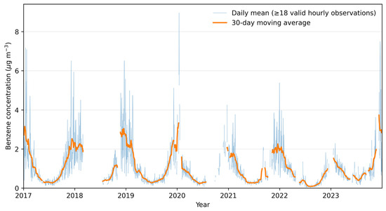
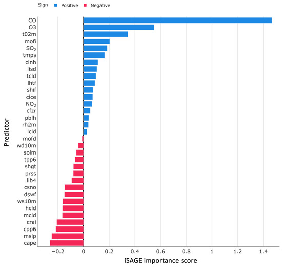
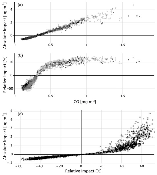
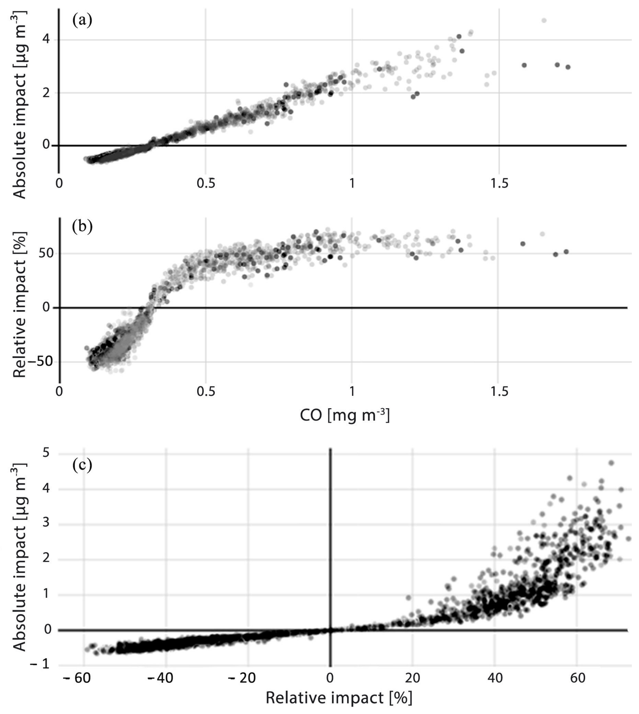
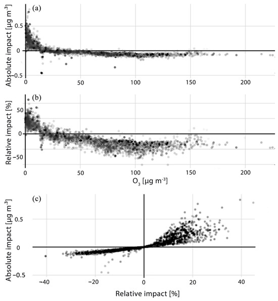
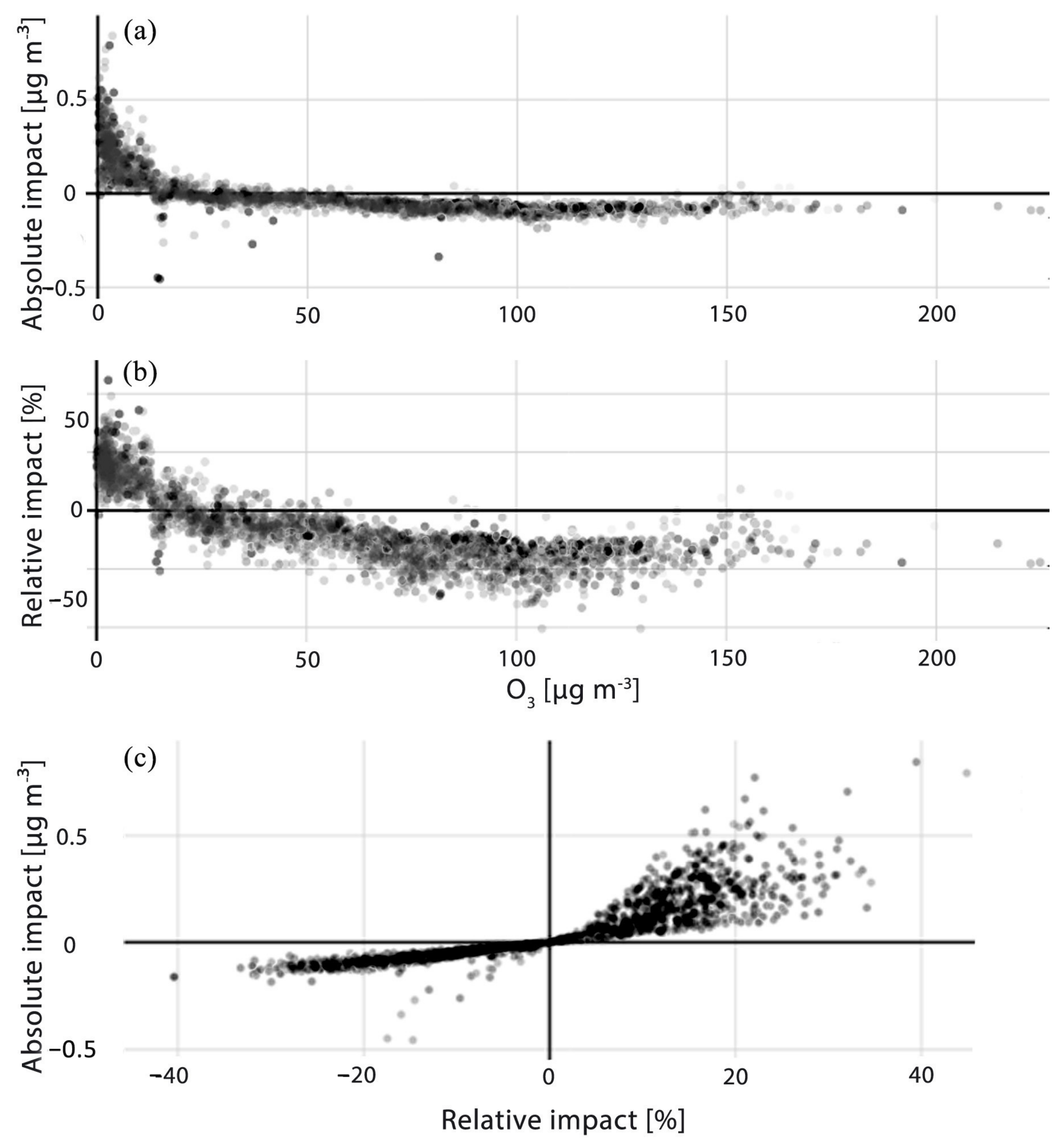
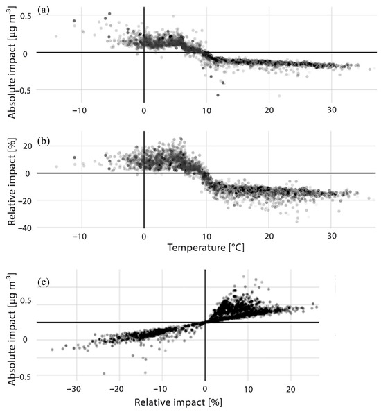
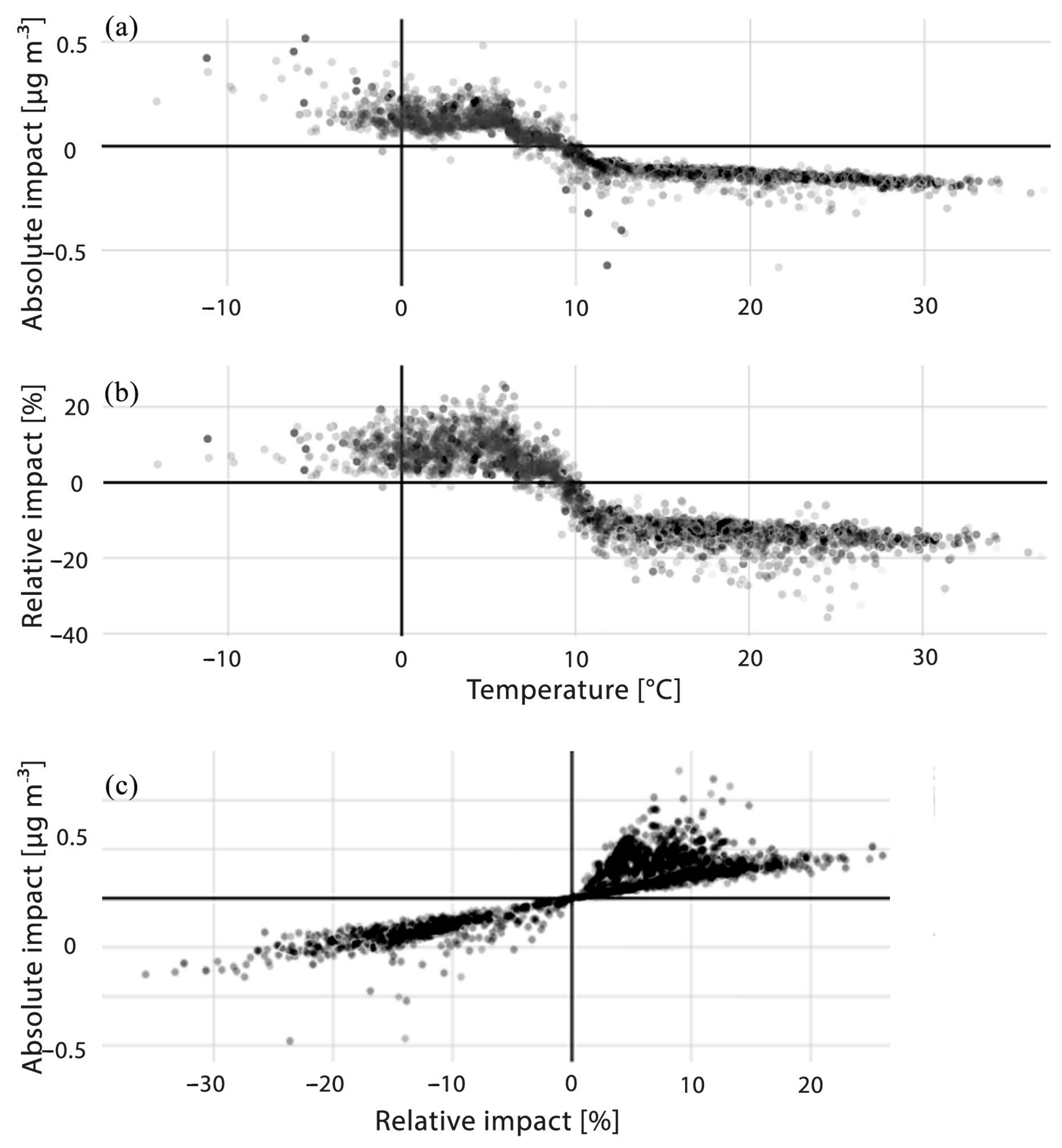

Disclaimer/Publisher’s Note: The statements, opinions and data contained in all publications are solely those of the individual author(s) and contributor(s) and not of MDPI and/or the editor(s). MDPI and/or the editor(s) disclaim responsibility for any injury to people or property resulting from any ideas, methods, instructions or products referred to in the content. |
© 2026 by the authors. Licensee MDPI, Basel, Switzerland. This article is an open access article distributed under the terms and conditions of the Creative Commons Attribution (CC BY) license.