


Abstract
Working from home (WFH) may reduce commuting and congestion, but additional non-work-related trips and household energy use may outweigh such environmental benefits. We examine whether annual changes in WFH prevalence are associated with changes in atmospheric CO2 concentration and tropospheric NO2 column density across U.S. metropolitan areas. We combine U.S. Census Bureau WFH data with satellite observations within 20 miles of each metropolitan area’s downtown center, yielding 216 metropolitan-year observations across 108 metropolitan areas in 2022 and 2023. We find that changes in WFH prevalence are not significantly associated with changes in atmospheric CO2 concentration. For NO2, the pooled regression shows a significant negative association with changes in WFH prevalence, although this association is statistically insignificant after including year fixed effects. Year-specific analyses reveal a more nuanced relation: the association is negative and statistically significant in 2021–2022 but turns positive and marginally significant in 2022–2023. This temporal variation may reflect shifts in the relative effects of reduced commuting and increased non-work-related travel, although we do not directly examine these potential mechanisms. We also caution that these estimates are conditional associations rather than causal effects, and are subject to satellite sampling and measurement limitations. Overall, the findings suggest that WFH’s environmental benefits vary across environmental outcomes and may depend on the extent of WFH adoption and associated changes in travel behavior. The results highlight the importance of considering workplace arrangements and their implications for travel patterns when developing urban transportation strategies to improve air quality.
1. Introduction
The rise of working from home (WFH) represents one of the most persistent changes in urban life following the COVID-19 pandemic [1], with important implications for public policy and corporate decision-making [2]. The feasibility of remote work varies substantially across occupations, industries, and cities [3], resulting in considerable geographical variation in WFH prevalence. By reducing the need to commute to centralized workplaces and allowing for greater flexibility in work schedules, WFH reshapes the spatial and temporal distribution of employees’ daily travel [4,5]. Understanding whether and to what extent WFH is associated with improvements in urban environmental quality is therefore important for informing corporate workplace policies and urban transportation and environmental planning.
The conventional argument for the environmental benefits of WFH centers on its potential to reduce commuting-related travel and associated emissions. Transportation accounts for approximately 28% of U.S. greenhouse gas emissions [6], making changes in commuting behavior potentially important for environmental outcomes. In 2019, approximately 119.2 million U.S. workers drove alone to their workplace, traveling an average of 27.6 min [7] and 16 miles [8] each way. Given the scale of daily commuting, even modest reductions in commuting frequency could translate into substantial reductions in aggregate vehicle travel and associated emissions. Moreover, by reducing the number of vehicles on urban roads during peak hours, WFH may also alleviate traffic congestion and its associated environmental impacts. Consistent with these potential benefits, Tao et al. [9] estimate that fully remote workers generate 54% fewer carbon emissions than fully onsite workers, with reductions of 11% to 29% for employees working from home two to four days per week and only 2% for those working from home one day per week. Similarly, Zheng et al. [10] estimate that a 10% reduction in onsite workers relative to the pre-pandemic level could reduce transportation-sector carbon emissions by 10%. Although both studies suggest potential environmental benefits from WFH, their estimates are not directly comparable because they differ in their working arrangements, behavioral assumptions, and environmental outcomes examined. These differences highlight the importance of examining the environmental implications of WFH, using observed atmospheric conditions in this study, to complement prior research based on estimated emission reductions.
Despite the potential environmental benefits, reduced commuting does not necessarily translate into proportional reductions in overall travel or transportation-related emissions. The flexibility provided by WFH may induce behavioral adjustments that partially offset the environmental benefits of reduced commuting. For example, employees may use the time saved from commuting to make additional trips for shopping, recreation, childcare, and other non-work activities [11,12]. Greater workplace flexibility may also allow employees to relocate farther from employment centers, potentially increasing travel distances on days when they commute. In addition, reduced commuting demand may lead to lower public transit ridership and greater reliance on private vehicles [4,5,10]. These behavioral responses highlight an important distinction between ongoing WFH arrangements and the initial COVID-19 lockdowns, during which widespread restrictions on mobility coincided with substantial reductions in air pollution [13,14]. As these restrictions were lifted, total annual vehicle mileage rebounded, approaching the pre-pandemic level by 2022 (Appendix A) [15]. Although this rebound cannot be attributed directly to WFH, it suggests that the environmental improvements observed during lockdowns may not persist under less restrictive workplace arrangements. Furthermore, the extent to which additional travel offsets commuting reductions may depend on the frequency of WFH. Prior evidence indicates that travel patterns differ across telework frequencies, suggesting that the environmental implications of WFH may vary with its intensity rather than increasing proportionally with its adoption [16].
In addition to changes in travel behavior, WFH may influence environmental outcomes by altering patterns of energy consumption across workplaces and residences. While reduced office occupancy has the potential to lower energy demand in commercial buildings, employees working from home may increase residential energy consumption for heating, cooling, lighting, and other activities. These additional household energy demands may partially or fully offset energy savings from reduced office use, particularly when commercial buildings continue to operate at relatively high energy levels despite lower occupancy. Consistent with this possibility, Hook et al. [17] document mixed evidence on whether teleworking reduces overall energy consumption, with the net effects depending on employee behavior, building efficiency, local climate, and related infrastructure. Although the digital technologies required to support remote work also consume energy, Tao et al. [9] estimate that their contribution to the overall carbon footprint is relatively small. Taken together, these considerations suggest that the environmental implications of WFH extend beyond reductions in commuting and depend on combined effects of changes in travel behavior and energy consumption. Consequently, whether WFH leads to measurable improvements in urban environmental conditions remains an empirical question.
Existing research provides evidence on several dimensions of teleworking’s environmental implications. Prior studies have estimated carbon footprints using commuting, building energy use, and information technology [9,17]; examined transportation-related outcomes such as vehicle mileage and transit ridership [4,10]; and documented changes in air pollution during the initial COVID-19 lockdowns [13,14]. However, the improvements in air quality observed during the lockdowns coincided with widespread restrictions on mobility and economic activity, making it difficult to isolate the environmental implications of WFH from those of broader pandemic-related disruptions. Our study complements and extends this evidence by examining the association between annual changes in WFH prevalence across U.S. metropolitan areas and changes in CO2 and NO2 concentrations in the post-pandemic period. By focusing on a period when commuting patterns continued to be influenced by WFH while other economic and social activities had largely resumed, our study provides evidence on the environmental implications of WFH under more typical mobility conditions, beyond those observed during the initial pandemic lockdowns.
To investigate this relationship, we combine WFH data from the U.S. Census Bureau with satellite-derived measures of atmospheric CO2 and NO2 concentration across U.S. metropolitan areas. Using data from 108 metropolitan areas in 2022 and 2023, we examine whether annual changes in WFH prevalence are associated with corresponding changes in these atmospheric measures. Unlike studies that estimate environmental impacts based on assumed reductions in commuting or changes in energy consumption, our approach examines observed atmospheric conditions, providing complementary evidence on the environmental implications of WFH. Importantly, CO2 and NO2 differ in their atmospheric characteristics and responsiveness to local emission sources. CO2 remains in the atmosphere for extended periods and is widely mixed, whereas NO2 has a relatively short atmospheric lifetime and is more sensitive to nearby combustion activities, including vehicle traffic [18,19,20,21]. Although neither measure directly captures locally generated emissions, and NO2 can originate from sources other than transportation, examining both pollutants allows us to assess whether the associations between WFH prevalence and observed atmospheric conditions vary by pollutant.
Our results reveal distinct associations between WFH prevalence and the two atmospheric outcomes. We find no statistically significant association between annual changes in WFH prevalence and changes in atmospheric CO2 concentrations. In contrast, changes in WFH prevalence are significantly negatively associated with changes in tropospheric NO2 column density in the pooled regression, and this association remains significant after controlling for metropolitan economic growth, population growth, and state-level greenhouse-gas-reduction targets. However, the association becomes statistically insignificant after including year fixed effects, indicating sensitivity to common year-specific changes. To further explore the temporal variation in this relationship, we conduct separate analyses for the 2021–2022 and 2022–2023 periods. The results show a more nuanced relation: a significant negative association in 2021–2022 but a positive association that is marginally statistically significant in 2022–2023, a period characterized by a further decline in WFH prevalence. These results underscore the importance of accounting for year effects and examining the periods separately when interpreting a pooled association.
One possible explanation for the differing results across year-specific regressions is that, when WFH prevalence is lower, reductions in commuting may provide limited congestion relief, while additional non-work travel may outweigh those reductions. However, we do not directly observe commuting patterns or traffic congestion, and satellite-derived NO2 measurements capture emissions from multiple sources beyond road transportation. Moreover, other economic and environmental conditions may have changed between the two periods. Therefore, although these findings suggest that the relationship between WFH and NO2 may vary over time, they do not establish that declining WFH prevalence has caused the change in the observed association or that a minimum level of WFH adoption is necessary to achieve environmental benefits.
This study contributes to the literature on remote work and urban sustainability by connecting post-pandemic changes in WFH prevalence to satellite-observed atmospheric outcomes across metropolitan areas. While prior studies document substantial improvements in environmental quality during the initial COVID-19 lockdowns, our findings provide complementary evidence from a period during which broad mobility restrictions had been lifted and WFH prevalence was declining. The differing associations observed for CO2 and NO2 underscore the importance of distinguishing among environmental outcomes when assessing the potential benefits of remote work. Moreover, the variation in the relationship between WFH and NO2 across years, which is obscured in the pooled analysis, suggests that its environmental implications may depend on broader changes in workplace arrangements and travel behavior. From a policy perspective, these findings highlight the need for employers and urban planners to consider not only reductions in commuting but also potential adjustments in non-work-related travel and residential and workplace energy consumption when evaluating the environmental implications of WFH.
2. Materials and Methods
2.1. Research Setting and Sample Construction
We examine changes in environmental conditions across U.S. metropolitan areas following the substantial expansion of WFH during the COVID-19 pandemic. Metropolitan areas provide an appropriate unit of analysis because commuting networks, employment centers, residential locations, and transportation infrastructure generally extend beyond municipal and county boundaries. WFH prevalence also varies considerably across metropolitan areas due to differences in occupational composition, employer practices, and local economic conditions. This variation allows us to examine whether annual changes in WFH prevalence are associated with annual changes in atmospheric conditions across metropolitan areas during the post-pandemic period.
We construct our sample by combining three primary data sources. We obtain metropolitan-level employment and commuting information, including the percentage of workers who work from home, from the U.S. Census Bureau. Metropolitan Statistical Areas (MSAs) are defined by the U.S. Office of Management and Budget (OMB) and consist of central counties containing an urban core with a population of at least 50,000, along with surrounding counties that exhibit substantial economic integration with the core, primarily through commuting patterns. We obtain atmospheric CO2 measurements from the Orbiting Carbon Observatory-2 (OCO-2), a satellite mission managed by NASA’s Jet Propulsion Laboratory (JPL, Pasadena, CA, USA). Atmospheric NO2 measurements are obtained from the European Space Agency (ESA)’s Tropospheric Monitoring Instrument (TROPOMI), which is jointly developed by the Netherlands and ESA. We geographically match the satellite observations to U.S. metropolitan areas and aggregate measurements within a 20-mile radius of each metropolitan area’s downtown center. This radius represents a practical balance between capturing a broader area of commuting-related activity and maintaining a geographically focused measure of urban atmospheric conditions. We then merge these environmental measures with the Census data and other metropolitan-level control variables used in our empirical analyses. To assess the sensitivity of our findings to the geographic coverage of satellite observations, Section 3.4 presents additional analyses using alternative radii of 10 and 30 miles.
Our sample covers 2022 and 2023, a period following the removal of most pandemic-related travel restrictions during which WFH remained substantially more prevalent than before the pandemic. This post-pandemic setting allows us to examine whether changes in realized WFH prevalence across metropolitan areas are associated with changes in observed environmental conditions after widespread lockdowns had been lifted. We first obtain metropolitan-level population data from the U.S. Census Bureau’s American Community Survey (ACS) 1-year estimates. We then collect annual data on the percentage of employed individuals working from home (WFH) from the ACS 1-year estimates. We restrict our sample to metropolitan areas with populations exceeding 500,000 to focus on relatively large urban areas where commuting activities and associated transportation emissions are more concentrated. Applying this criterion yields 109 metropolitan areas. We further exclude Honolulu, Hawaii, because its geographical isolation and distinctive atmospheric conditions may limit its comparability with metropolitan areas in the contiguous United States. Specifically, Honolulu’s tropical maritime climate, prevailing trade winds, and island-specific atmospheric circulation patterns may affect the transport and dispersion of atmospheric pollutants differently than conditions in mainland metropolitan areas [22]. After this exclusion, our final sample consists of 108 metropolitan areas and 216 annual observations.
2.2. Measurement of Working from Home
We measure WFH using data from the U.S. Census Bureau’s American Community Survey (ACS). The ACS asks employed individuals aged 16 years and older how they usually traveled to work during the preceding week. Respondents who select “worked from home” are classified as home-based workers. For each metropolitan area and year, we calculate WFH as the percentage of workers who report working from home. Thus, the measure captures the prevalence of realized WFH arrangements among workers in a metropolitan area rather than the availability of WFH policies announced by individual employers. Higher values of WFH indicate that a larger proportion of the metropolitan workforce primarily performs its work from home.
The ACS measure offers several advantages for our analysis. It is constructed consistently across metropolitan areas, covers a broad and nationally representative population, and reflects workers’ actual work locations rather than stated preferences or the technical feasibility of remote work. Nevertheless, the measure has important limitations. Because the ACS records respondents’ usual means of commuting, it does not report the exact number of days worked from home and may classify hybrid employees according to where they work most frequently. Consequently, metropolitan-level WFH prevalence may underestimate the proportion of workers who work remotely at least occasionally and may not fully capture changes in remote-work frequency among hybrid workers. Moreover, the ACS estimates might be subject to sampling errors. Thus, although the ACS uses a consistent classification across metropolitan areas, these limitations may introduce measurement error to our measure of metropolitan-level WFH prevalence. Finally, these data also do not distinguish between WFH initiated by employers and WFH chosen by employees, identify the policies of individual employers, or capture the variation in work arrangement. Accordingly, WFH should be interpreted as a metropolitan-level measure of realized WFH prevalence, rather than a direct measure of employer WFH policy or individual remote-work intensity.
2.3. Measurement of Environmental Outcomes
We examine two satellite-derived environmental outcomes: atmospheric CO2 and NO2 concentrations. Using both measures is important because they capture different dimensions of the environmental effects associated with changes in WFH prevalence. CO2 is a long-lived greenhouse gas generated by transportation, electricity production, building energy use, and other economic activities. It therefore provides a broad atmospheric measure potentially reflecting total energy consumption and travel. In contrast, NO2 is a short-lived, spatially concentrated air pollutant produced primarily by fuel combustion, including emissions from cars, trucks, buses, power plants, and off-road equipment [18]. It provides a measure that is particularly responsive to motor-vehicle traffic and congestion in urban areas [23,24], and exposure to traffic-related NO2 has been associated with increased lung-cancer risk [25]. However, satellite-observed NO2 column density captures contributions from multiple emission sources and does not distinguish road traffic from other sources. Examining the two measures together allows us to assess whether changes in WFH prevalence are associated with different atmospheric outcomes, without identifying the specific activities responsible for those associations.
To ensure data quality, we first apply the quality-control criteria specified for each satellite retrieval product to identify valid observations. We rely on the OCO-2 Version 11 Level 2 full-physics retrieval product and retain only CO2 observations flagged as good in the dataset and NO2 observations with a quality assurance value greater than 0.75 for the following analysis. We then calculate daily average concentrations only, focusing on days with at least 10 valid retrievals within the selected geographical area. Annual concentrations are subsequently calculated as the equally weighted average of these qualifying daily means. This approach ensures that days with more valid satellite retrievals do not receive disproportionate weight in the annual estimates.
2.3.1. CO2 Measurement
We obtain atmospheric CO2 data from NASA’s Orbiting Carbon Observatory-2 (OCO-2), a satellite launched to observe the geographical distribution of carbon dioxide in the Earth’s atmosphere [19]. OCO-2 uses high-resolution spectrometers to measure the absorption of sunlight reflected from the Earth’s surface in wavelength bands associated with oxygen and CO2. These spectral observations are used to retrieve the column-averaged dry-air mole fraction of carbon dioxide, commonly denoted as XCO2 and expressed in parts per million [19]. XCO2 represents the average CO2 concentration throughout the atmospheric column above an observed location, rather than the amount of CO2 emitted directly at the location. We assign the available satellite observations to metropolitan areas based on their geographical coordinates. We aggregate observations within the downtown-centered area using the daily and annual averaging procedures described in the previous section. Our resulting measure, CO2, captures the average atmospheric CO2 concentration observed for each metropolitan area during the corresponding year.
The OCO-2 measure is useful because it provides consistently constructed observations of atmospheric CO2 across geographical areas without requiring us to estimate emissions from assumed commuting behavior, fuel consumption, or residential energy use. It therefore allows us to examine whether metropolitan areas with different levels of WFH also exhibit different observed CO2 concentrations. However, XCO2 is not a direct measure of locally generated emissions. Atmospheric CO2 concentrations reflect emissions from multiple sources, natural carbon uptake and release, and the transportation of air across geographical boundaries [20]. In addition, clouds, aerosols, surface characteristics, and uneven terrain can prevent valid satellite retrievals and produce uneven coverage across metropolitan areas and time [19]. Aggregating the available observations to the metropolitan-year level reduces the influence of individual retrievals but does not eliminate these limitations. Small changes in urban CO2 concentrations associated with WFH may also be difficult to detect against variations in background concentrations, particularly given OCO-2’s limited spatial and temporal coverage. Accordingly, our CO2 measure captures broad atmospheric conditions associated with metropolitan activity but cannot attribute observed concentrations specifically to commuting or other behavioral changes caused by WFH.
2.3.2. NO2 Measurement
We obtain atmospheric NO2 data from the TROPOMI aboard the European Union’s Copernicus Sentinel-5 Precursor satellite [24]. We use the TROPOMI Processor Version 2 Level 2 product consistently across all study years, retaining observations with quality-assurance values greater than 0.75. TROPOMI measures sunlight reflected by the Earth’s surface and atmosphere across spectral bands that permit the retrieval of several atmospheric constituents, including NO2. We use its estimate of tropospheric NO2 vertical column density, with a measurement unit of 1015 molecules/cm2, which represents the amount of NO2 contained in a vertical column of the troposphere over an observed location [21]. We assign satellite observations to metropolitan areas based on their geographical coordinates and aggregate observations within the downtown-centered area using the daily and annual averaging procedures described previously. Our resulting measure, NO2, captures the average tropospheric NO2 column density observed for each metropolitan area during the corresponding year. Prior urban research similarly uses TROPOMI observations to examine spatial and temporal variation in air pollution [26] and reports that NO2 is more sensitive to traffic volume and congestion [23,24].
The TROPOMI measure is particularly useful for our research question because NO2 is closely associated with fuel combustion and varies spatially with urban traffic and other localized economic activity [18]. Its relatively short atmospheric lifetime makes tropospheric NO2 column density more sensitive than XCO2 to changes in nearby emission-generating activities, including changes in concentrated commuter traffic. TROPOMI’s broad geographical coverage and consistent measurement process also facilitate comparisons across metropolitan areas [21,26]. Nevertheless, the measure has several limitations. TROPOMI observes NO2 throughout the tropospheric column rather than directly measuring ground-level exposure or vehicle emissions. Observed NO2 may originate from power generation, industrial production, off-road equipment, wildfires, and other sources in addition to road traffic [18]. Retrievals are also affected by cloud cover, surface reflectivity, atmospheric conditions, and assumptions used to separate tropospheric from stratospheric NO2 [21]. Accordingly, our NO2 measure captures tropospheric pollution from multiple emission sources, and it cannot isolate the portion attributable to road traffic or determine whether changes in commuting behavior explain its association with WFH prevalence. We also acknowledge that TROPOMI’s approximately 13:30 local overpass does not directly capture morning peak commuting conditions. Although atmospheric observations at this time may reflect residual effects of earlier emissions, the extent of these effects depends on atmospheric transport, mixing, and chemical processes. Consequently, our satellite measurements do not provide direct evidence of reductions in morning commuting or traffic congestion.
Finally, tropospheric NO2 column density is influenced by meteorological conditions, including wind, temperature, boundary-layer height, and solar radiation, which affect atmospheric transport, mixing, and chemistry processes. Appendix C presents descriptive comparisons of ECMWF ERA5 meteorological measures between 2019 and 2021–2023. Within each metropolitan group, mean surface radiation, air temperature, wind speed, and boundary layer height are broadly similar across the two periods. However, these group-level comparisons provide only descriptive context and do not capture annual meteorological variation across individual metropolitan areas. To address this variation, we include annual changes in these four variables as additional controls in the robustness tests reported in Section 3.4. We acknowledge that other meteorological conditions could also contribute to differences in NO2 across metropolitan areas. Finally, we acknowledge that wildfire emissions and smoke transport may also affect observed NO2 levels, while smoke aerosols can introduce uncertainty into satellite retrievals.
2.4. Empirical Model
We estimate the association between changes in WFH prevalence and changes in atmospheric conditions at the metropolitan-area level. We construct separate regression models for CO2 and NO2 because the two measures capture different dimensions of environmental quality and may respond differently to changes in commuting and other activities associated with WFH. Our primary specification relates the annual change in each environmental outcome to the annual change in WFH prevalence and includes metropolitan-level control variables.
In Equation (1), represents the annual percentage change in either atmospheric CO2 concentration or tropospheric NO2 column density for metropolitan area in year . is the annual percentage change in metropolitan WFH prevalence, calculated as 100 × (WFHt − WFHt−1)/WFHt−1. and are the annual percentage changes in metropolitan GDP and population, respectively. These variables control for the changes in the scale of economic activity and population that may affect both transportation activity and atmospheric conditions. is an indicator variable equal to one if the state containing the metropolitan area has established a greenhouse-gas-reduction target, and zero otherwise. Nevertheless, we acknowledge that these controls may not fully account for other potentially relevant factors, including changes in public-transit investment, local transportation-emission regulations, and industry or occupational composition. The estimated coefficients on should therefore be interpreted as conditional associations rather than causal effects. We report robust standard errors clustered by metropolitan areas to account for correlation in the regression residuals within metropolitan areas over time. In untabulated tests, we conduct additional analyses using state-clustered standard errors. These analyses allow for within-state residual correlation across neighboring metropolitan areas. The results remain the same.
The coefficient of interest, , captures whether metropolitan areas with greater changes in WFH prevalence experience larger or smaller annual changes in the corresponding environmental outcome. A negative coefficient indicates that metropolitan areas with positive changes in WFH experience smaller increases, or greater decreases, in atmospheric CO2 or NO2. Because WFH prevalence is not randomly assigned and may be associated with unobserved metropolitan characteristics, we interpret as a conditional association rather than a definitive causal effect.
We include annual growth in metropolitan GDP and population as control variables because changes in economic activity and population may affect both WFH prevalence and atmospheric conditions. Growth in economic activity may increase transportation, commercial energy use, and industrial production, thereby contributing to changes in CO2 and NO2. Controlling for these variables helps distinguish the association between WFH prevalence and environmental outcomes from changes attributable to metropolitan economic and population growth. We include whether the metropolitan area is in a state with a GHG-reduction target because state climate commitments may be accompanied by transportation, energy, or emissions policies that independently affect atmospheric CO2 and NO2 concentrations. Controlling for the presence of such a target helps distinguish the association with changes in WFH prevalence from broader state differences in environmental policy. For metropolitan areas spanning multiple states, we assign state-level climate policy characteristics based on the jurisdiction of the metropolitan area’s principal city. For example, the Washington metropolitan area is assigned to Washington, D.C., which has established its own GHG-reduction targets. We acknowledge that this approach does not fully capture differences in climate policies across jurisdictions within the same metropolitan area.
We further estimate the specifications separately for the 2021–2022 and 2022–2023 periods. In each subsample, the coefficient on captures the association between changes in WFH prevalence and changes in the atmospheric outcome across metropolitan areas, conditional on the included controls. This approach allows the estimated association to differ between the two periods rather than imposing a common coefficient across years. However, because WFH prevalence and other post-pandemic conditions evolve over time, differences in annual estimates do not necessarily indicate that the relationship depends on a particular level of WFH prevalence.
3. Results
3.1. Geographical Evidence
Before presenting the regression results, we provide visual illustrations of atmospheric CO2 and NO2 patterns across metropolitan areas with different levels of WFH prevalence. These comparisons offer descriptive context for companies, employers, and urban planners. We classify metropolitan areas using their average percentage of workers working from home from 2021 to 2023. The ten metropolitan areas with the highest average percentages constitute the most flexible group, while the ten with the lowest percentages constitute the least flexible group. WFH prevalence ranges from approximately 20% to 30% among the most flexible metropolitan areas but is no greater than approximately 10% among the least flexible metropolitan areas. This contrast provides a descriptive setting for examining whether metropolitan areas with substantially different levels of workplace flexibility exhibit different environmental patterns.
Figure 1A compares the annual average atmospheric CO2 concentrations between the most and least flexible metropolitan areas from 2017 to 2023. Before the pandemic, the two groups exhibited similar CO2 concentrations: the 2017–2019 average was 409.82 parts per million (ppm) among the most flexible metropolitan areas and 409.30 ppm among the least flexible metropolitan areas. CO2 concentrations subsequently increased in both groups, reaching post-2020 averages of 416.26 ppm and 416.54 ppm, respectively. The similar levels and trends do not suggest that metropolitan areas with greater WFH prevalence experienced meaningfully different changes in atmospheric CO2.
Figure 1.
Atmospheric CO2 and NO2 Concentrations in Metropolitan Areas with the Highest and Lowest WFH Prevalence. Panel (A) presents annual average atmospheric CO2 concentrations from 2017 to 2023 for the ten metropolitan areas with the highest average WFH prevalence and the ten metropolitan areas with the lowest average WFH prevalence. The two groups are identified using average WFH prevalence from 2021 to 2023, as reported in Table 1. CO2 concentration is measured in parts per million within a 20-mile radius of each metropolitan area’s downtown center using observations from NASA’s Orbiting Carbon Observatory-2 satellite. Panel (B) presents annual average tropospheric NO2 column densities from 2018 to 2023 for the ten metropolitan areas with the highest average WFH prevalence and the ten metropolitan areas with the lowest average WFH prevalence. The two groups are identified using average WFH prevalence from 2021 to 2023, as reported in Table 1. NO2 column density is measured in units of 1015 molecules per square centimeter within a 20-mile radius of each metropolitan area’s downtown center using observations from the Tropospheric Monitoring Instrument aboard the European Space Agency’s Sentinel-5 Precursor satellite. Panel (C) compares annual average atmospheric CO2 concentrations and tropospheric NO2 column densities between the ten metropolitan areas with the highest average WFH prevalence and the ten metropolitan areas with the lowest average WFH prevalence. The two groups are identified using average WFH prevalence from 2021 to 2023, as reported in Table 1. For each environmental measure and metropolitan group, the average concentration observed before 2020 is normalized to one, and the annual values from 2020 to 2023 are scaled relative to that benchmark. Values above one indicate an increase relative to the corresponding pre-2020 average, whereas values below one indicate a decrease.
Figure 1B presents the corresponding trends in tropospheric NO2 concentrations. In contrast to the relatively similar CO2 trends across the two groups, NO2 exhibits substantial differences. From 2019 to 2020, average NO2 decreased by 1.11 × 10¹⁵ molecules/cm2 among the most flexible metropolitan areas but remained nearly unchanged among the least flexible metropolitan areas, with an average change of 0.03 × 10¹⁵ molecules/cm2. From 2021 to 2023, NO2 concentrations remained relatively stable in most of the most flexible metropolitan areas, with Austin being a notable exception. NO2 concentrations increased in nearly all the least flexible metropolitan areas over the same period. These patterns provide preliminary evidence that WFH prevalence may be more closely associated with variation in tropospheric NO2 than with broader atmospheric CO2 concentrations.
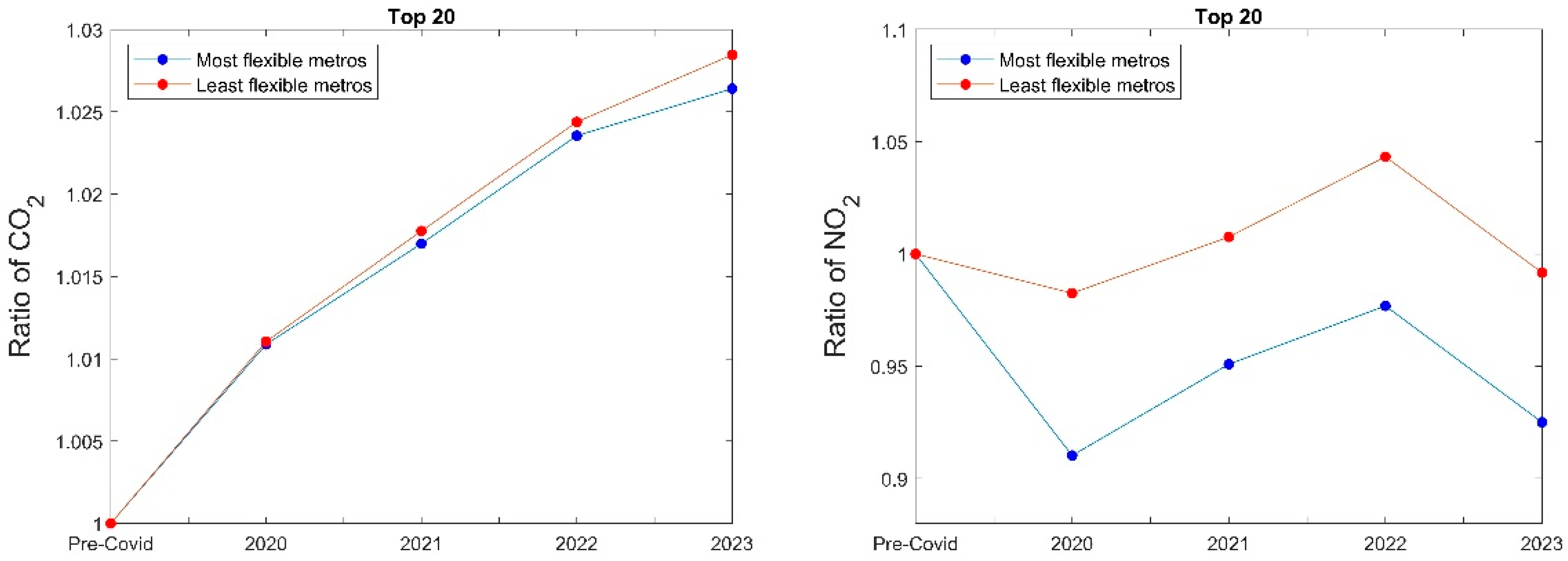
Figure 1C facilitates comparison by scaling each group’s annual average concentration relative to its pre-2020 average. During our sample period of 2021–2023, the NO2 series display more pronounced differences in trajectories between the high- and low-WFH groups than the CO2 series, which follow similar upward paths. The historical observations show that this contrast was also apparent during the initial pandemic period, when NO2 exhibited more pronounced departures from its pre-pandemic baseline than did CO2. These plots provide descriptive context for the different CO2 and NO2 results reported below. The lockdown-era observations are included for historical context rather than as evidence of the post-lockdown WFH association examined in our regressions. The change in CO2 does not differ significantly between the most and least flexible metropolitan areas (t(18) = −0.877, p = 0.392), consistent with the trends shown in Figure 1A. In contrast, the difference in NO2 changes between the two groups is statistically significant (t(18) = −4.025, p < 0.01). Thus, the normalized comparisons reinforce the descriptive evidence that differences in WFH prevalence are more clearly reflected in NO2 than in CO2. We also present the corresponding analysis using the 20 metropolitan areas with the highest WFH prevalence and the 20 metropolitan areas with the lowest WFH prevalence in Appendix B, and the inferences are the same.
Figure 2 illustrates the spatial distribution of NO2 concentrations in 2020 and 2023 across the most and least flexible metropolitan areas. The difference maps use blue to indicate decreases in NO2 concentrations between the two years and red to indicate increases. Increases are observed in metropolitan areas in both groups, which is not surprising given the unusually low NO2 concentrations during the initial COVID-19 lockdowns in 2020. Notably, several of the most flexible metropolitan areas exhibit decreases around their downtown areas, whereas more than half of the least flexible metropolitan areas exhibit increases.
Figure 2.
Satellite Images of NO2 Concentration in the Highest WFH (Most Flexible) and Lowest WFH (Least Flexible) Metros. Panel (A) presents satellite-derived tropospheric NO2 column densities in 2020 and 2023 for each of the ten metropolitan areas with the highest average WFH prevalence. The black star identifies the downtown center of each metropolitan area. In the annual concentration maps, colors progressing from blue to red represent increasing NO2 column density. The difference maps report the change from 2020 to 2023: red areas indicate increases in NO2, while blue areas indicate decreases. Several metropolitan areas exhibit decreases in NO2 around their downtown centers over this period. These maps only provide descriptive illustrations of spatial changes in NO2 rather than a test of their association with changes in WFH prevalence. They also do not account for concurrent changes in local environmental policies or other metropolitan-level factors. Panel (B) presents satellite-derived tropospheric NO2 column densities in 2020 and 2023 for each of the ten metropolitan areas with the lowest average WFH prevalence. The black star identifies the downtown center of each metropolitan area. In the annual concentration maps, colors progressing from blue to red represent increasing NO2 column density. The difference maps report the change from 2020 to 2023: red areas indicate increases in NO2, while blue areas indicate decreases. More than half of these metropolitan areas exhibit increases in NO2 around their downtown centers over this period. These maps only provide descriptive illustrations of spatial changes in NO2 rather than a test of their association with changes in WFH prevalence. They also do not account for concurrent changes in local environmental policies or other metropolitan-level factors.
Overall, Figure 1 and Figure 2 provide visual comparisons of average CO2 and NO2 concentrations across metropolitan groups, but do not establish whether changes in NO2 concentrations are associated with changes in WFH prevalence. The persistence of NO2 below its pre-pandemic baseline in the high-WFH group, compared with its return toward the baseline in the low-WFH group, is broadly consistent with a negative relationship between WFH prevalence and NO2 concentrations. Nevertheless, these descriptive comparisons cover different time periods, do not control for other factors that may influence atmospheric conditions, and are limited to the ten metropolitan areas with the highest and lowest WFH prevalence. The following regression analyses provide a more systematic and direct examination of the association between annual changes in WFH prevalence and annual changes in atmospheric conditions during 2021–2023, while controlling for other relevant factors.
3.2. Descriptive Statistics
Table 1 reports annual WFH prevalence for the metropolitan areas included in the two groups. Among the most flexible metropolitan areas, average WFH prevalence decreased from 30.68% in 2021 to 24.72% in 2022 and 21.28% in 2023. Average WFH prevalence was substantially lower and more stable among the metropolitan areas with the lowest WFH prevalence, decreasing from 9.24% in 2021 to 8.29% in 2022 and 8.22% in 2023. Thus, although WFH prevalence generally declined after the initial pandemic period, a substantial difference between the two groups of metropolitan areas persisted throughout the three-year period. This sustained contrast provides the basis for the comparisons of atmospheric CO2 and NO2 concentrations presented in Figure 1 and Figure 2. Furthermore, the decline in WFH prevalence provides important context for the subsample analyses by year.
Table 1.
WFH Prevalence in the Highest and Lowest WFH Metropolitan Areas. Panel (A): Percentage of Remote Workers in the Highest WFH Metros. Panel (B): Percentage of Remote Workers in the Lowest WFH Metros.
Table 2 presents descriptive statistics and Pearson correlations for the variables used in the regression analyses. The sample contains 216 metropolitan-year observations representing 108 metropolitan areas in 2022 and 2023. As reported in Panel A, atmospheric CO2 concentrations increased by an average of 0.436% annually, whereas tropospheric NO2 concentrations decreased by an average of 1.246%. The mean annual change in WFH prevalence is −9.440%, indicating that the percentage of workers working from home generally declined as metropolitan areas moved further beyond the initial pandemic period. Nevertheless, the standard deviation of 9.206% indicates substantial variation in this change across metropolitan areas and years. Given the generally negative changes in WFH prevalence during our sample period, a higher ΔWFH generally represents a smaller percentage decline in WFH prevalence. Accordingly, a negative coefficient on ΔWFH in our regression analysis would indicate that metropolitan areas with smaller percentage declines in WFH prevalence tend to exhibit smaller increases, or larger decreases, in the atmospheric outcome, holding other factors constant. Metropolitan GDP and population increased by averages of 2.775% and 1.111% annually, respectively. In addition, 57.4% of the metropolitan-year observations are from states with a GHG-reduction target.
Table 2.
Descriptive Statistics and Correlation. Panel (A): Descriptive Statistics. Panel (B): Pearson Correlation Matrix.
In Panel B of Table 2, we report the Pearson correlations. These univariate associations indicate that changes in WFH prevalence are negatively associated with changes in tropospheric NO2, but they are not significantly associated with changes in atmospheric CO2 concentrations. The correlations among the explanatory variables are generally modest, with the largest being 0.464 between GDP growth and population growth. Thus, the correlation matrix does not indicate substantial concerns about multicollinearity. Because these correlations do not account for other metropolitan characteristics, we next examine these relationships using multivariate regression analyses.
3.3. WFH Prevalence and Changes in Environmental Outcomes
Table 3 presents the regression results examining the association between annual changes in WFH prevalence and annual changes in atmospheric conditions. We first discuss the results related to CO2. Panel A presents the results of the pooled regression. Columns (1) and (3) use the annual percentage change in CO2 concentration as the dependent variable. Column (1), which includes ΔWFH as the only explanatory variable, reports a coefficient of approximately zero that is not statistically significant. In Column (3), the coefficient on ΔWFH remains statistically insignificant after controlling for GDP growth, population growth, and the presence of a state GHG-reduction target. We do not detect a statistically significant association between annual changes in WFH prevalence and annual changes in atmospheric CO2 in this sample. Panel B presents the results of estimating the model separately by year. As reported in Columns (1) and (2), the CO2 coefficients remain statistically insignificant in both periods.
Table 3.
Association between ∆WFH and Changes in CO2 and NO2 Concentrations. Panel (A): Pooled regression. Panel (B): Regression by year.
We now turn our attention to the results for NO2. In the pooled regression reported in Panel A of Table 3, Columns (2) and (4) examine annual changes in tropospheric NO2. In Column (2), the coefficient on ΔWFH is −0.129 and statistically significant (p-value = 0.007). In economic terms, a one-standard-deviation increase in ΔWFH is associated with a decrease in ∆NO2 equivalent to approximately 17.94% of its standard deviation. After controlling for GDP growth, population growth, and the presence of a state GHG-reduction target in Column (4), the coefficient on ΔWFH increases in magnitude to −0.164 and remains statistically significant. This coefficient indicates that a one-percentage-point increase in ΔWFH is associated with a 0.164-percentage-point decrease in ΔNO2, holding other factors constant. In economic terms, a one-standard-deviation increase in ΔWFH is associated with a decrease in ∆NO2 equivalent to approximately 22.81% of its standard deviation. The relatively low R2 values indicate the limited explanatory power of our regression models. We acknowledge that changes in atmospheric CO2 and NO2 concentrations are influenced by numerous factors beyond WFH prevalence, including meteorological conditions, industrial activity, transportation patterns, and other emission sources that may not be fully captured by our models. Nevertheless, our primary objective is to examine the association between changes in WFH prevalence and atmospheric conditions rather than to predict overall changes in atmospheric concentrations.
To assess whether the pooled results are sensitive to common year-specific factors, we re-estimate the pooled specification with year fixed effects. The coefficient on ΔWFH becomes statistically insignificant, suggesting that the negative association observed in the baseline pooled regression may partly reflect differences across years. Alternatively, the loss of significance may reflect differences in the direction of the association across the two periods, with opposing effects potentially offsetting each other in the pooled estimation. These possibilities motivate our separate analysis of the two periods.
In Panel B, the analysis by year indicates that the NO2 results are more nuanced. In Column (3), the coefficient on ΔWFH is −0.154 for the 2021–2022 period and statistically significant at the 5% level. In Column (4), the coefficient becomes positive at 0.110 and is significant at the 10% level for the 2022–2023 period. In other words, the negative association observed in the pooled regression does not hold consistently across periods. Instead, the association is negative and statistically significant in 2021–2022 but positive and marginally statistically significant in 2022–2023. In contrast, the association between changes in WFH prevalence and atmospheric CO2 concentrations remains statistically insignificant in both the pooled and year-specific analyses.
One possible explanation for the negative association between ΔWFH and changes in NO2 is that metropolitan areas with greater increases in WFH experienced slower economic growth, which independently reduced transportation activity and air pollution. To examine this possibility, Table 4 reports regressions using annual metropolitan GDP growth as the dependent variable. Column (1) shows that ΔWFH is positively associated with GDP growth, with a coefficient of 0.051 that is statistically significant at the 1% level. After controlling for population growth in Column (2), the coefficient decreases to 0.024 but remains statistically significant at the 10% level. In other words, metropolitan areas with greater increases, or smaller decreases, in WFH prevalence experienced higher rather than lower economic growth. However, these pooled results do not suggest that slower GDP growth explains the observed relationship between changes in WFH prevalence and changes in NO2 concentrations. We acknowledge that potential confounding effects arising from industry composition or sector-specific changes in economic activity and emissions cannot be ruled out.
Table 4.
Changes in WFH and GDP Growth.
In summary, the analyses reveal different associations across atmospheric outcomes and time periods. The association between annual changes in WFH and annual changes in CO2 concentration remains statistically insignificant. For NO2, the significant negative pooled association becomes statistically insignificant after including year fixed effects. Subsample analyses reveal that the negative association is concentrated in 2021–2022 and becomes positive and marginally statistically significant in 2022–2023. Section 4 discusses the explanations and implications of these findings.
3.4. Robustness Tests
In robustness tests, we examine whether our findings are sensitive to the spatial radius used to construct the satellite-derived atmospheric measures. We repeat the analyses using satellite observations within a 10-mile and 30-mile radius of each metropolitan area’s downtown center, compared with the 20-mile radius used in the main analyses. We present these results in Table 5. Panel A reports the pooled regression results using a 10-mile radius. In Columns (1) and (3), the coefficients on ΔWFH remain statistically insignificant for CO2. In contrast, the coefficients on ΔWFH for NO2 in Columns (2) and (4) remain negative and statistically significant at the 1% level. When control variables are included, the coefficient on ΔWFH is −0.182, as reported in Column (4).
Table 5.
Robustness tests. Panel (A): Pooled regression using CO2 and NO2 concentrations measured within 10 miles of each metropolitan area’s downtown. Panel (B): Year-specific regression using CO2 and NO2 concentrations measured within 10 miles of each metropolitan area’s downtown. Panel (C). Pooled regression using CO2 and NO2 concentrations measured within 30 miles of each metropolitan area’s downtown. Panel (D): Year-specific regression using CO2 and NO2 concentrations measured within 30 miles of each metropolitan area’s downtown. Panel (E): Pooled regression controlling for meteorological conditions. Panel (F). Year-specific regressions controlling for meteorological conditions.
Panel C of Table 5 reports the corresponding pooled regression results using a 30-mile radius. Consistent with the main analyses, the coefficients on ΔWFH remain statistically insignificant for CO2 in Columns (1) and (3), while the NO2 coefficients are negative and significant at the 1% level, as reported in Columns (2) and (4). Specifically, the coefficient on ΔWFH is −0.193 in Column (4), which includes all the control variables. Moreover, the magnitudes of the NO2 coefficients are comparable across the 10-mile, 20-mile, and 30-mile specifications, both with and without control variables. In conclusion, our results from the pooled regression are robust to alternative geographical radii.
Panel B and Panel D of Table 5 report the year-specific regression results using 10-mile and 30-mile radii, respectively. In both panels, the coefficients on ΔWFH for CO2 remain statistically insignificant, as reported in Columns (1) and (2). For NO2, Panel B shows that the coefficient on ΔWFH is −0.168 and statistically significant at the 5% significance level shown for 2021–2022 (Column 3), while the coefficient is positive (0.108) at the 10% significance level for 2022–2023 (Column 4). These findings are consistent with the main results reported in Table 3 using a 20-mile radius. When the radius is expanded to 30 miles, as Panel D shows, the coefficient on ΔWFH remains negative (−0.169) and statistically significant at the 1% level for 2021–2022 (Column 3). However, although the coefficient remains positive for 2022–2023, it is no longer statistically significant (Column (4)), in contrast to the marginally significant positive associations observed under the 10-mile and 20-mile specifications.
We further examine whether these results are sensitive to annual changes in metropolitan meteorological conditions. Panel E of Table 5 reports the results of our pooled regressions after controlling for annual changes in surface solar radiation, air temperature, wind speed, and boundary-layer height. The coefficient on ΔWFH for NO2 remains negative but decreases in magnitude from −0.164 to −0.079 and is statistically significant at the 10% level. Panel F presents the results of our year-specific analyses with these additional meteorological controls. In Columns (3) and (4), the coefficient on ΔWFH is −0.158 for 2021–2022 and 0.114 for 2022–2023, respectively, both statistically significant at the 5% level. These findings suggest that the negative association in the pooled regression and the opposing associations across the two periods persist after accounting for meteorological conditions. In addition, the coefficients on ΔWFH for CO2 remain statistically insignificant in both the pooled and year-specific analyses.
Overall, these robustness analyses indicate that the absence of a statistically significant association between changes in WFH prevalence and CO2, as well as the negative NO2 associations in the pooled sample and the 2021–2022 subsample, are robust to alternative geographic radii. In contrast, the positive NO2 association in 2022–2023 is less consistent across specifications, remaining marginally significant at the 10% level under the 10-mile and 20-mile radii but becoming statistically insignificant under the 30-mile radius. Additional analyses controlling for annual changes in meteorological conditions, including surface solar radiation, air temperature, wind speed, and boundary layer height, further support the main findings. Taken together, these findings highlight the importance of considering temporal variation, geographic measurement choices, and meteorological conditions when interpreting the associations between WFH prevalence and atmospheric NO2 concentrations.
4. Discussion
4.1. Discussion of Main Findings and Environmental Implications
This study examines whether post-pandemic changes in WFH prevalence are associated with changes in atmospheric CO2 concentration and tropospheric NO2 column density across U.S. metropolitan areas. We find no statistically significant association between changes in WFH prevalence and CO2 in either the pooled or year-specific analyses. Regarding NO2, the negative association in the pooled analysis becomes statistically insignificant after including year fixed effects. The year-specific analyses show that the association is negative in 2021–2022, but becomes positive and marginally significant in 2022–2023. The robustness tests using alterative radius indicate that these patterns are not confined to the baseline 20-mile measurement area. Moreover, the variation across years provides a more nuanced interpretation of the findings: an average association across the post-pandemic adjustment period does not necessarily describe the relationship in each stage of the adjustment period. Together, these results highlight the importance of considering both atmospheric outcomes and the period under study when evaluating the environmental implications of WFH prevalence. Reduced commuting and associated congestion relief represent one plausible explanation for the negative NO2 association, which we discuss further below.
The absence of a detectable association with CO2 is consistent with the possibility that reductions in commuting are offset by other behavioral and energy-use responses. Employees working from home may make additional non-work trips, reside farther from employment centers, or travel longer distances on the days they commute [4,5,10]. WFH may also shift energy consumption from shared office buildings to individual residences, and the resulting environmental effect depends on building efficiency, climate, household behavior, and the energy sources used to generate electricity [9,17]. Moreover, atmospheric CO2 reflects emissions from numerous local and nonlocal sources as well as natural carbon processes and atmospheric transport. Consequently, changes in commuting may be too small relative to these broader influences to produce a detectable change in metropolitan-level CO2, particularly given OCO-2’s limited spatial and temporal sampling. The null result therefore should not be interpreted as evidence that WFH has no effect on transportation behavior, but rather that a significant association with atmospheric CO2 is not detected in our sample.
Several factors may explain differences between our findings and those of prior studies (Tao et al.; Zheng et al.). First, reductions in transportation-related emissions may not translate proportionally into changes in atmospheric concentrations, which are also influenced by meteorological conditions, atmospheric transport, and emissions from other sources. Second, changes in non-work travel, residential energy consumption, and workplace energy use may offset some of the potential environmental benefits of reduced commuting. Third, our analysis focuses on the post-pandemic period, when WFH prevalence and travel behavior was continuing to adjust following the initial lockdowns. Accordingly, the absence of a statistically significant association between WFH and atmospheric CO2 does not necessarily contradict prior estimates of potential emissions reductions.
The negative association between changes in WFH prevalence and tropospheric NO2 column density provides a different perspective on the environmental implications of WFH. Because NO2 is short-lived and concentrated near combustion sources, urban NO2 concentrations are generally more responsive than CO2 concentrations to changes in vehicle traffic and congestion [18,20,23,24]. Reduced concentrated commuting and associated congestion relief therefore represent a plausible explanation for the observed association. WFH arrangements may reduce traffic volumes along major commuting corridors during peak periods, even if employees subsequently make shorter or more dispersed trips at other times. Less congested traffic could reduce NO2 emissions associated with vehicle idling and stop-and-go traffic. However, our analyses do not directly measure changes in commuting patterns or traffic congestion, and satellite-observed NO2 concentrations are also influenced by emissions from power generation, industrial activity, and other combustion sources. Therefore, we cannot directly verify this proposed mechanism with the available data. Nevertheless, to the extent that reduced concentrated commuting explains the association, the findings suggest that the timing and concentration of travel may influence urban air quality alongside total travel.
The year-specific analyses further show that the association between changes in WFH prevalence and NO2 differs in direction across the two periods, shifting from negative in 2021–2022 to positive in 2022–2023. One possible explanation is that, when WFH prevalence is lower, WFH-related commuting reductions provide limited congestion relief, while additional non-work travel may offset or even outweigh those reductions. However, this explanation remains speculative, as our data do not allow us to identify the factors underlying the observed reversal.
Prior research suggests that the environmental implications of WFH may depend on remote-work frequency and associated travel behavior. Caldarola and Sorrell [16] find that most teleworkers travel farther weekly than non-teleworkers, but more frequent teleworking is associated with lower private travel. Similarly, Tao et al. [9] estimate substantially different carbon benefits across remote-work frequencies. However, these findings concern individual working arrangements and do not establish a threshold for WFH prevalence at the metropolitan level. Moreover, the substantial pollution reductions documented during the initial COVID-19 lockdowns [13,14] occurred alongside widespread restrictions on mobility and economic activity, making it difficult to isolate the environmental effects of WFH from those of broader lockdown measures. Our year-specific results are consistent with the possibility that travel-related responses changed during the post-pandemic adjustment period, but other changes in economic activity, transportation patterns, and local conditions between the periods may also explain the reversal.
This study complements research on remote work and environmental sustainability. Prior studies estimate teleworking’s carbon footprint from commuting, building energy use, and information technology [9,17] or examine transportation outcomes such as vehicle mileage and transit ridership [4,10]. For example, Brodeur et al. [13] document reductions in PM2.5 following safer-at-home orders, while Cooper et al. [14] document substantial reductions in ground-level NO2 during the initial lockdowns. However, these studies examine periods characterized by widespread restrictions on mobility and economic activity. In contrast, our study focuses on a subsequent period in which WFH arrangements persisted after broader restrictions had largely been lifted. We find no significant association between changes in WFH and atmospheric CO2, while the association with tropospheric NO2 column density varies across the two annual periods. Together, these results suggest that environmental improvements accompanying broad lockdowns do not necessarily translate into consistent environmental benefits from WFH arrangements under post-lockdown conditions.
For urban planners and employers, the findings suggest that WFH does not necessarily deliver consistent environmental benefits simply because it reduces the need to commute. Its environmental implications are better understood in the context of specific objectives: our analysis detects no significant association with atmospheric CO2, while the NO2 association varies across the two sample years. To the extent that traffic congestion relief explains the negative association between WFH and NO2 in 2021–2022, flexible workplace arrangements and staggered commuting schedules could complement congestion-management strategies. Evaluating these applications requires evidence on whether commuting reductions alleviate peak-period traffic, whether additional travel offsets those reductions, and how energy consumption shifts between workplaces and homes. The appropriate role of WFH in environmental planning therefore depends on both the outcome being targeted and the behavioral changes accompanying its implementation.
4.2. Limitations and Future Research
This study has several limitations that provide opportunities for future research. First, the regression sample covers only 2022 and 2023 because consistent metropolitan-level WFH data are unavailable for 2020 and begin only in 2021. The short sample period limits our ability to examine longer-term changes in workplace arrangements, residential location, transportation infrastructure, and travel behavior. This limitation also constrains our ability to identify the factors underlying variation in the WFH−NO2 association across years. Because declining WFH prevalence has coincided with broader changes in economic activity and travel behavior, we cannot determine whether the change in the observed association is attributable to declining WFH prevalence or establish a minimum level of WFH prevalence necessary to generate environmental benefits. Second, WFH prevalence is not randomly assigned. Metropolitan areas experiencing different changes in WFH may also differ in industry composition, occupational structure, public transit availability, land-use patterns, environmental regulation, and other characteristics that affect air quality. Although our analyses control for economic growth, population growth, and state GHG-reduction targets, unobserved differences may still exist. The estimated coefficients should therefore be interpreted as conditional associations rather than definitive causal effects.
The measures also impose important limitations. First, the Census measure identifies workers who work from home but does not capture the number of remote-work days, differences between fully remote and hybrid arrangements, or the timing of employees’ travel. Second, the satellite outcomes measure atmospheric concentrations rather than emissions generated directly within each metropolitan area. XCO2 is affected by atmospheric transport and natural carbon processes, while satellite coverage for both gases may vary due to clouds, aerosols, and surface conditions. At the same time, aggregation to the metropolitan-year level also obscures variation across neighborhoods, seasons, and times of day. Third, the atmospheric measures cover downtown-centered areas, whereas WFH prevalence describes the metropolitan workforce. Although the alternative-radius analyses show the results are not sensitive to alternative geographical coverage of the atmospheric measures, they do not eliminate the potential spatial mismatch or establish which radius best represents the activities associated with WFH. Fourth, wildfire emissions and smoke transport may also affect observed NO2 levels, while smoke aerosols can introduce uncertainty into satellite retrievals. Finally, the analysis does not directly observe commuting, non-work travel, residential energy consumption, or traffic congestion and therefore cannot identify the specific behavioral mechanism underlying the NO2 association. Future research could combine more detailed workplace schedules with mobility, traffic, energy-use, and ground-level air-quality data to determine when, where, and through which activities WFH affects urban environments.
5. Conclusions
This study examines whether post-pandemic changes in WFH prevalence are associated with changes in atmospheric CO2 concentration and tropospheric NO2 column density across U.S. metropolitan areas. Using Census data on WFH prevalence and satellite-derived environmental observations, we find no statistically significant association between changes in WFH prevalence and CO2 in either the pooled or year-specific analyses. In contrast, increases in WFH prevalence are significantly associated with reductions in tropospheric NO2 column density in the pooled regression, but the association becomes statistically insignificant after including year fixed effects. Year-specific analyses further reveal a more nuanced relation: the coefficient on changes in WFH is negative and statistically significant in 2021–2022, but positive and marginally significant in 2022–2023. These findings suggest that the potential environmental benefits of WFH should be interpreted with caution, as the observed associations vary across atmospheric outcomes and time periods, potentially reflecting changes in WFH prevalence and other post-pandemic conditions.
Overall, our results complement prior research on the initial COVID-19 lockdowns by examining WFH after widespread mobility and economic restrictions had been lifted. The substantial pollution reductions documented during initial lockdowns do not necessarily translate into comparable benefits from WFH in the post-lockdown period. For urban planners, the findings highlight the importance of considering specific environmental objectives, as well as prevailing work and travel patterns, when evaluating the potential environmental implications of WFH arrangements.
Author Contributions
Conceptualization, M.M.; methodology, L.Z.; data curation, L.Z.; writing—original draft, B.B.X.; writing—review and editing, M.M., B.B.X. and L.Z.; supervision, M.M. All authors have read and agreed to the published version of the manuscript.
Funding
This research received no external funding.
Institutional Review Board Statement
Not applicable.
Informed Consent Statement
Not applicable.
Data Availability Statement
The original contributions presented in this study are included in the article. Further inquiries can be directed to the corresponding author. The public datasets used and extended figures and data tables for reproducibility will be available upon acceptance for publication.
Acknowledgments
We thank Lan Gao from the School of Meteorology at the University of Oklahoma for providing greenhouse gas concentration data and research assistance. We used Gen AI for grammar checking and proofreading.
Conflicts of Interest
The authors declare no conflicts of interest.
Appendix A. Annual Vehicle Miles
Figure A1.
Graph is taken from https://afdc.energy.gov/data/10315 (accessed on 20 June 2025). Original Source: Federal Highway Administration monthly Traffic Volume Trends report. Annual VMT values show moving 12-month averages taken in February of the listed year.
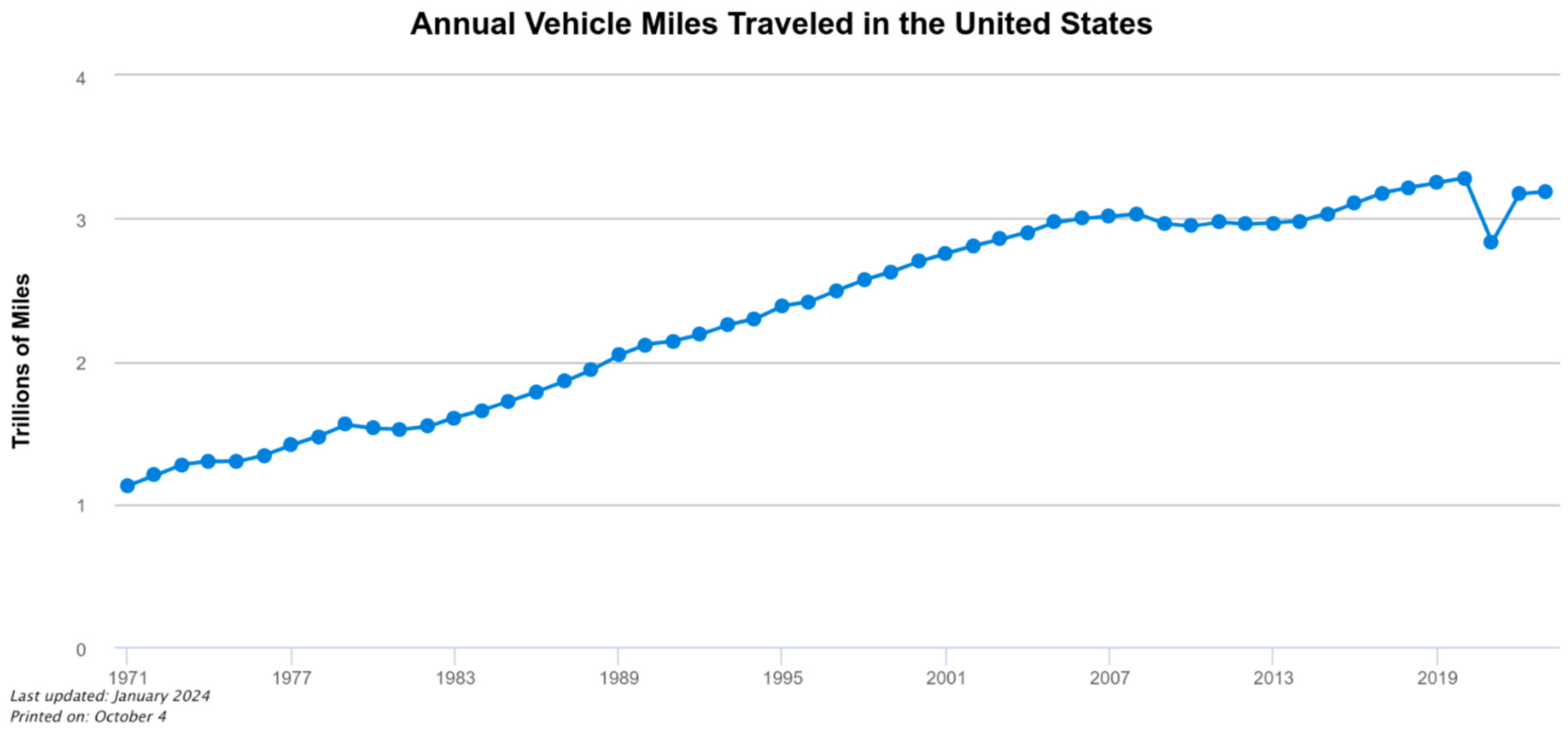
This chart shows trends in total vehicle miles traveled (VMT) in the United States (expressed as a moving 12-month count) from 1971 to 2023. The long rise in VMT has seen three periods of flattened growth or decline, triggered by the oil price spikes of 1974, 1979, and 2008. The VMT flattening that started in 2008 continued long after oil prices recovered, largely because of an economic recession. Starting in 2012, VMT began rising again largely because the U.S. economy recovered while petroleum prices remained relatively low. The rate of increase slowed between 2017 and 2020. Because of the COVID-19 pandemic, VMT in 2021, which reflects February 2020 through January 2021, was the lowest since 2002. VMT then rebounded to nearly pre-pandemic levels in 2022.
Appendix B. Comparisons of Annual Average CO2 and NO2 Between Highest 20 (Most Flexible) and Lowest 20 WFH (Least Flexible) Metros
Figure A2.
This figure compares annual average atmospheric CO2 concentrations and tropospheric NO2 column densities between the 20 metropolitan areas with the highest average WFH prevalence and the 20 metropolitan areas with the lowest average WFH prevalence. The two groups are identified using average WFH prevalence from 2021 to 2023. For each environmental measure and metropolitan group, the average concentration observed before 2020 is normalized to one, and the annual values from 2020 to 2023 are scaled relative to that benchmark. Values above one indicate an increase relative to the corresponding pre-2020 average, whereas values below one indicate a decrease.
Appendix C. Descriptive Comparison of Meteorological Conditions
Table A1.
This table reports mean meteorological conditions for the ten metropolitan areas with the highest average WFH prevalence, the ten with the lowest average WFH prevalence, and the full sample of 108 metropolitan areas. The pre-pandemic period is 2019, and the post-pandemic period covers 2021–2023. Meteorological data are obtained from the ECMWF ERA5 reanalysis, which provides hourly observations at a spatial resolution of 0.25° × 0.25°. The variables include surface solar radiation (watts per square meter), which measures incoming solar energy at the Earth’s surface; 2-m air temperature (Kelvin), which measures air temperature at 2 m above the surface; 10-m wind speed (meters per second), which measures horizontal wind speed at 10 m above the surface; and boundary-layer height (meters), which measures the vertical extent of the atmospheric boundary layer where surface emissions are mixed and dispersed.
References
- Barrero, J.M.; Bloom, N.; Davis, S.J. Why Working from Home Will Stick; NBER Working Paper No. 28731; NBER: Cambridge, MA, USA, 2026. [Google Scholar] [CrossRef] [Scilit]
- Council of Economic Advisers. Economic Report of the President; Executive Office of the President: Washington, DC, USA, 2025. Available online: https://www.govinfo.gov/content/pkg/ERP-2025/pdf/ERP-2025.pdf (accessed on 12 June 2025).
- Dingel, J.I.; Neiman, B. How many jobs can be done at home? J. Public Econ. 2020, 189, 104235. [Google Scholar] [CrossRef] [Scilit] [PubMed]
- Kappler, L.B.; Colaço, R.; Melo, P.C.; de Abreu e Silva, J. Will telework reduce travel? An evaluation of empirical evidence with meta-analysis. Urban Sci. 2025, 9, 199. [Google Scholar] [CrossRef] [Scilit]
- Rodrigues, E.H.d.S.d.B.T.; Turini, L.R.; Caetano, J.A.; Baltar, M.L.d.B.; de Oliveira, C.M.; Ribeiro, G.M.; Orrico Filho, R.D. Study into the impact of the pandemic on travel patterns within the Metropolitan Area of Rio de Janeiro. Urban Sci. 2024, 8, 103. [Google Scholar] [CrossRef] [Scilit]
- U.S. Environmental Protection Agency. Carbon Pollution from Transportation. Available online: https://www.epa.gov/transportation-air-pollution-and-climate-change/carbon-pollution-transportation (accessed on 10 June 2025).
- Burd, C.; Burrows, M.; McKenzie, B. Travel Time to Work in the United States: 2019; American Community Survey Reports, ACS-47; U.S. Census Bureau: Washington, DC, USA, 2021. Available online: https://www.census.gov/library/publications/2021/acs/acs-47.html (accessed on 25 May 2025).
- Bailey, J.R.; Cohen, A. That “Dreaded” Commute is Actually Good for Your Health. Harvard Business Review, 21 May 2021. Available online: https://hbr.org/2021/05/that-dreaded-commute-is-actually-good-for-your-health (accessed on 15 June 2025).
- Tao, Y.; Yang, L.; Jaffe, S.; Amini, F.; Bergen, P.; Hecht, B.; You, F. Climate mitigation potentials of teleworking are sensitive to changes in lifestyle and workplace rather than ICT usage. Proc. Natl. Acad. Sci. USA 2023, 120, e2304099120. [Google Scholar] [CrossRef] [Scilit] [PubMed]
- Zheng, Y.; Wang, S.; Liu, L.; Aloisi, J.; Zhao, J. Impacts of remote work on vehicle miles traveled and transit ridership in the USA. Nat. Cities 2024, 1, 346–358. [Google Scholar] [CrossRef] [Scilit]
- Shreedhar, G.; Laffan, K.; Giurge, L.M. Is Remote Work Actually Better for the Environment? Harvard Business Review, 7 March 2022. Available online: https://hbr.org/2022/03/is-remote-work-actually-better-for-the-environment (accessed on 12 June 2025).
- Finan, A.; Bloom, N. How Working from Home Boosted Golf; Stanford University: Stanford, CA, USA, 2023. Available online: https://nbloom.people.stanford.edu/sites/g/files/sbiybj24291/files/media/file/golfingfromhome.pdf (accessed on 25 May 2025).
- Brodeur, A.; Cook, N.; Wright, T. On the effects of COVID-19 safer-at-home policies on social distancing, car crashes and pollution. J. Environ. Econ. Manag. 2021, 106, 102427. [Google Scholar] [CrossRef] [Scilit] [PubMed]
- Cooper, M.J.; Martin, R.V.; Hammer, M.S.; Levelt, P.F.; Veefkind, P.; Lamsal, L.N.; Krotkov, N.A.; Brook, J.R.; McLinden, C.A. Global fine-scale changes in ambient NO2 during COVID-19 lockdowns. Nature 2022, 601, 380–387. [Google Scholar] [CrossRef] [Scilit] [PubMed]
- Federal Highway Administration. Traffic Volume Trends: December 2022; Office of Highway Policy Information, U.S. Department of Transportation: Washington, DC, USA, 2023. Available online: https://www.fhwa.dot.gov/policyinformation/travel_monitoring/22dectvt/22dectvt.pdf (accessed on 23 May 2025).
- Caldarola, B.; Sorrell, S. Do teleworkers travel less? Evidence from the English National Travel Survey. Transp. Res. Part A Policy Pract. 2022, 159, 282–303. [Google Scholar] [CrossRef] [Scilit]
- Hook, A.; Court, V.; Sovacool, B.K.; Sorrell, S. A systematic review of the energy and climate impacts of teleworking. Environ. Res. Lett. 2020, 15, 093003. [Google Scholar] [CrossRef] [Scilit]
- U.S. Environmental Protection Agency. Basic Information About NO2. Available online: https://www.epa.gov/no2-pollution/basic-information-about-no2 (accessed on 12 June 2025).
- Crisp, D.; Pollock, H.R.; Rosenberg, R.; Chapsky, L.; Lee, R.A.M.; Oyafuso, F.A.; Frankenberg, C.; O’Dell, C.W.; Bruegge, C.J.; Doran, G.B.; et al. The on-orbit performance of the Orbiting Carbon Observatory-2 (OCO-2) instrument and its radiometrically calibrated products. Atmos. Meas. Tech. 2017, 10, 59–81. [Google Scholar] [CrossRef] [Scilit]
- Mitchell, K.A.; Doney, S.C.; Keppel-Aleks, G. Characterizing average seasonal, synoptic, and finer variability in Orbiting Carbon Observatory-2 XCO2 across North America and adjacent ocean basins. J. Geophys. Res. Atmos. 2023, 128, e2022JD036696. [Google Scholar] [CrossRef] [Scilit] [PubMed]
- van Geffen, J.; Eskes, H.; Compernolle, S.; Pinardi, G.; Verhoelst, T.; Lambert, J.-C.; Sneep, M.; ter Linden, M.; Ludewig, A.; Boersma, K.F.; et al. Sentinel-5P TROPOMI NO2 retrieval: Impact of version v2.2 improvements and comparisons with OMI and ground-based data. Atmos. Meas. Tech. 2022, 15, 2037–2060. [Google Scholar] [CrossRef] [Scilit]
- Baker, K.R.; Nguyen, T.K.V.; Sareen, N.; Henderson, B.H. Meteorological and air quality modeling for Hawaii, Puerto Rico, and Virgin Islands. Atmos. Environ. 2020, 234, 117543. [Google Scholar] [CrossRef] [Scilit] [PubMed]
- Wang, Y.; Liu, P.; Schwartz, J.; Castro, E.; Wang, W.; Chang, H.; Scovronick, N.; Shi, L. Disparities in ambient nitrogen dioxide pollution in the United States. Proc. Natl. Acad. Sci. USA 2023, 120, e2208450120. [Google Scholar] [CrossRef] [Scilit] [PubMed]
- Gantt, B.; Owen, R.C.; Watkins, N. Characterizing nitrogen oxides and fine particulate matter near major highways in the United States using the National Near-Road Monitoring Network. Environ. Sci. Technol. 2021, 55, 2831–2838. [Google Scholar] [CrossRef] [Scilit] [PubMed]
- Hamra, G.B.; Laden, F.; Cohen, A.J.; Raaschou-Nielsen, O.; Brauer, M.; Loomis, D. Lung cancer and exposure to nitrogen dioxide and traffic: A systematic review and meta-analysis. Environ. Health Perspect. 2015, 123, 1107–1112. [Google Scholar] [CrossRef] [Scilit] [PubMed]
- Hanami, Z.A.; Amin, M.; Hustim, M.; Putri, R.M.; Torabi, S.E.; Ramadhani, A.A.T.; Suryati, I. Spatial–temporal changes in air pollutants in four provinces of Sumatra Island, Indonesia: Insights from Sentinel-5P satellite imagery. Urban Sci. 2025, 9, 42. [Google Scholar] [CrossRef] [Scilit]
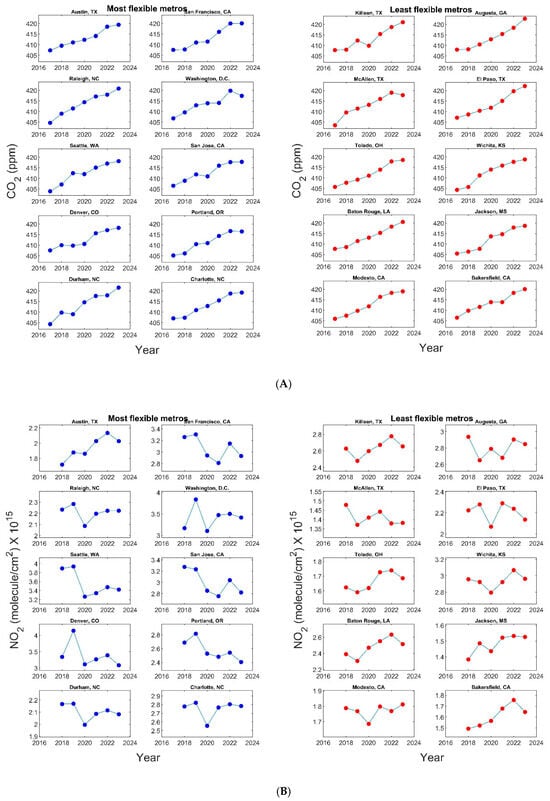
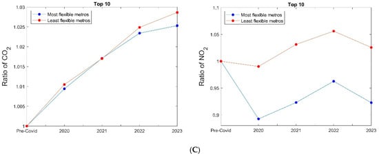
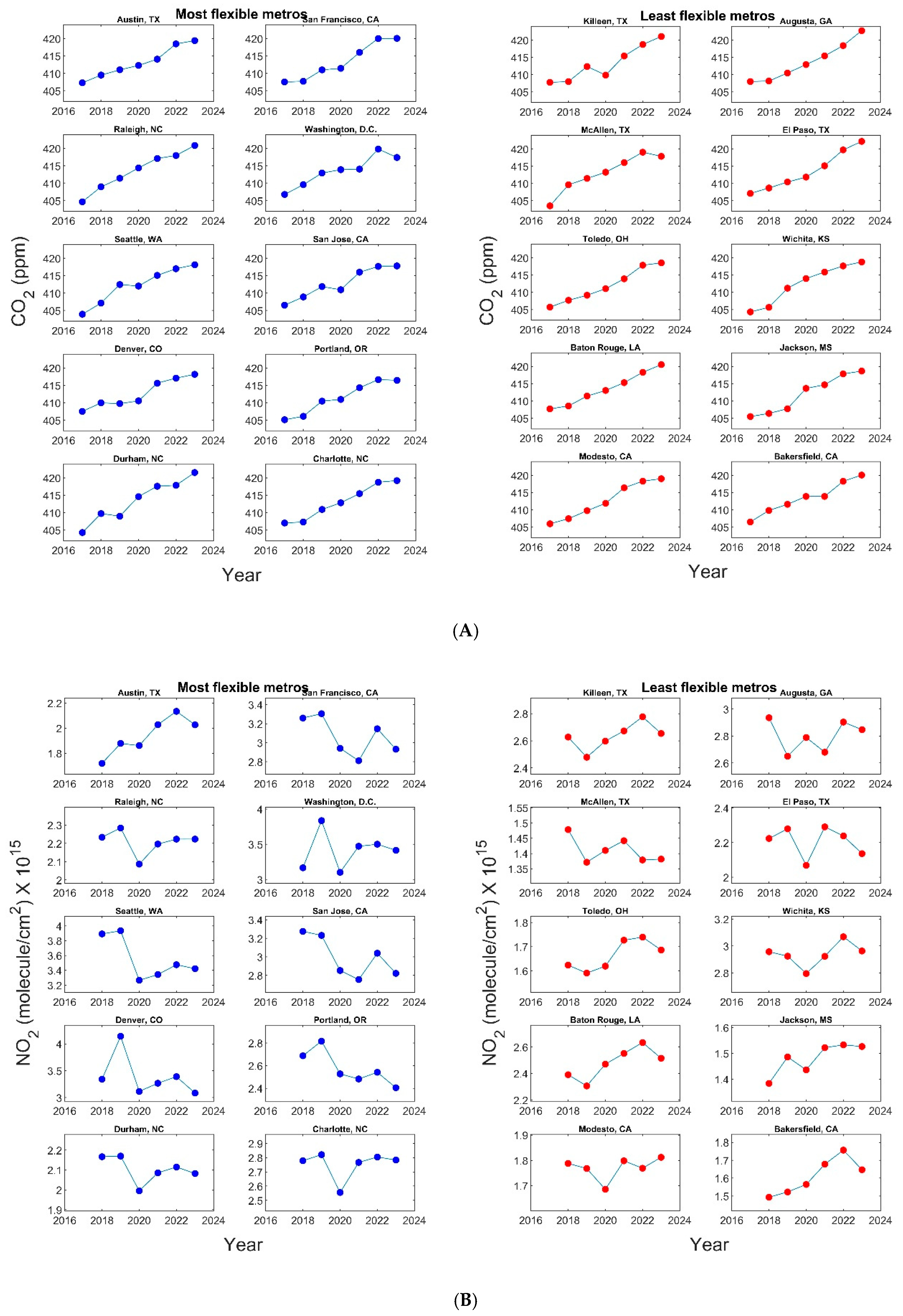
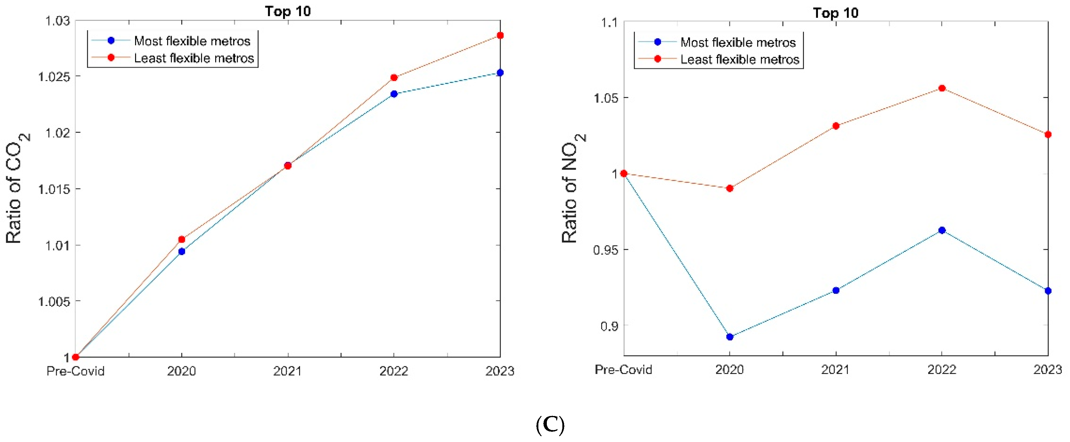
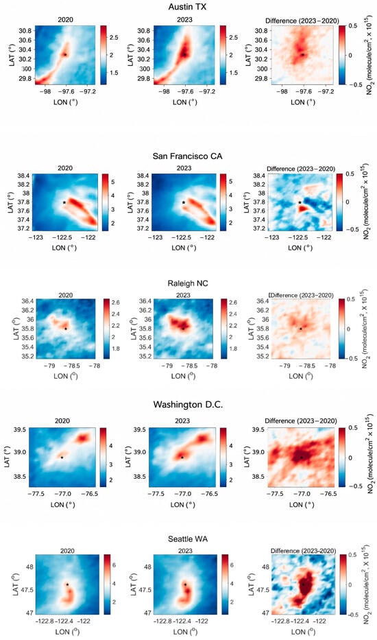
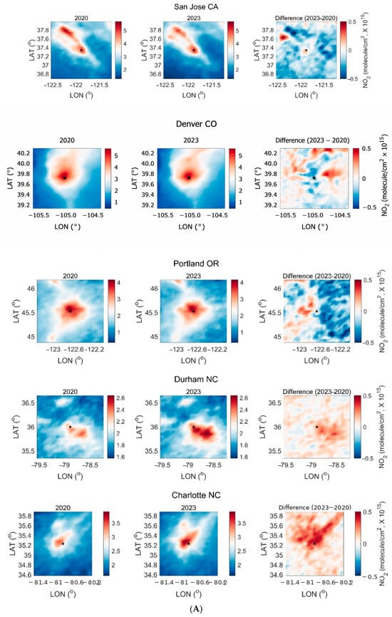
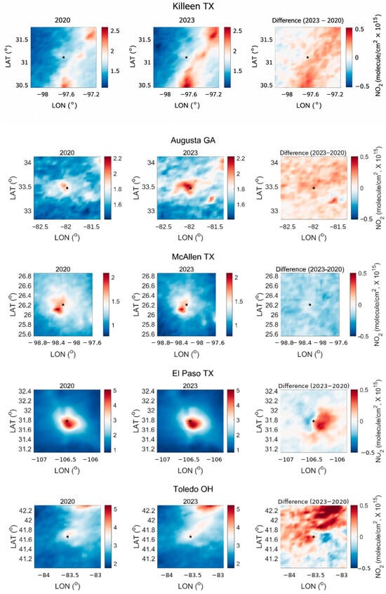
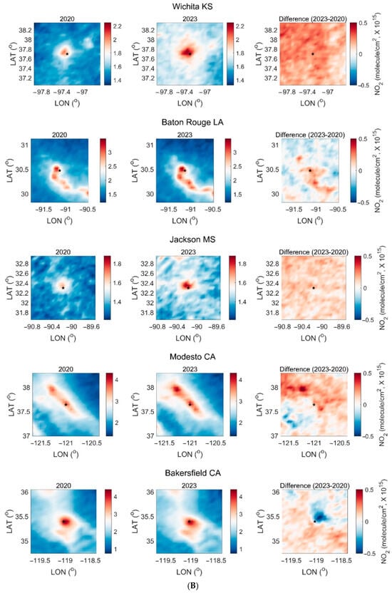
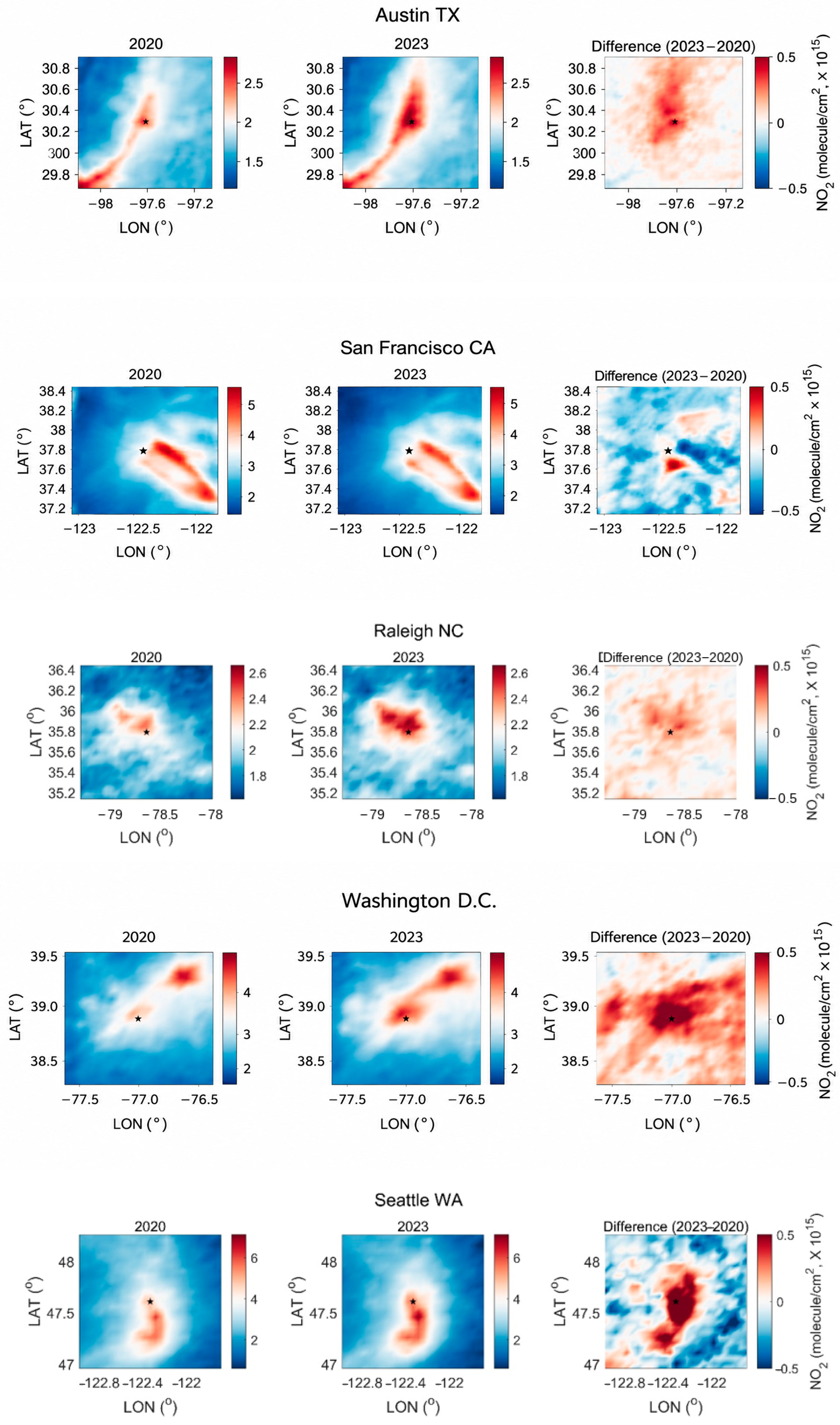
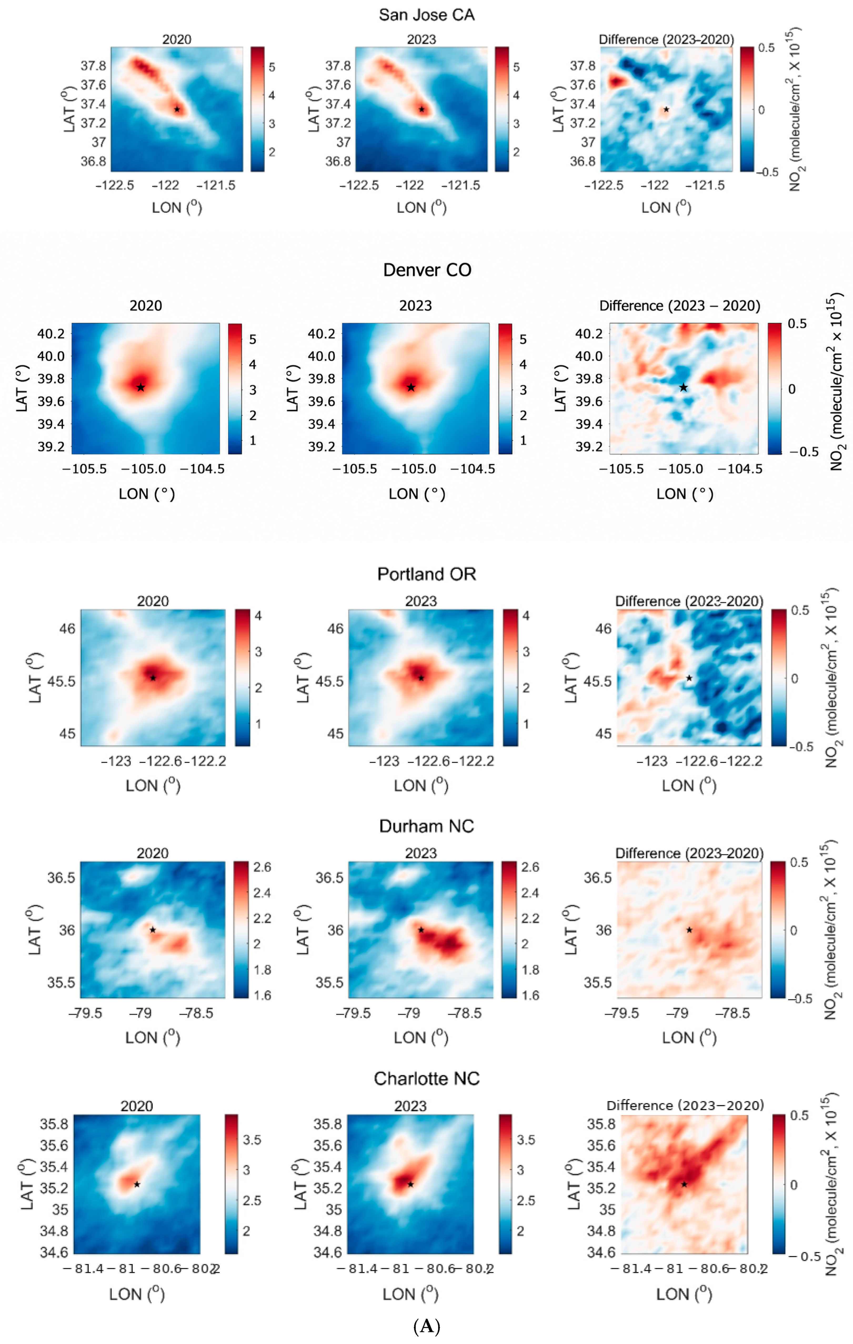
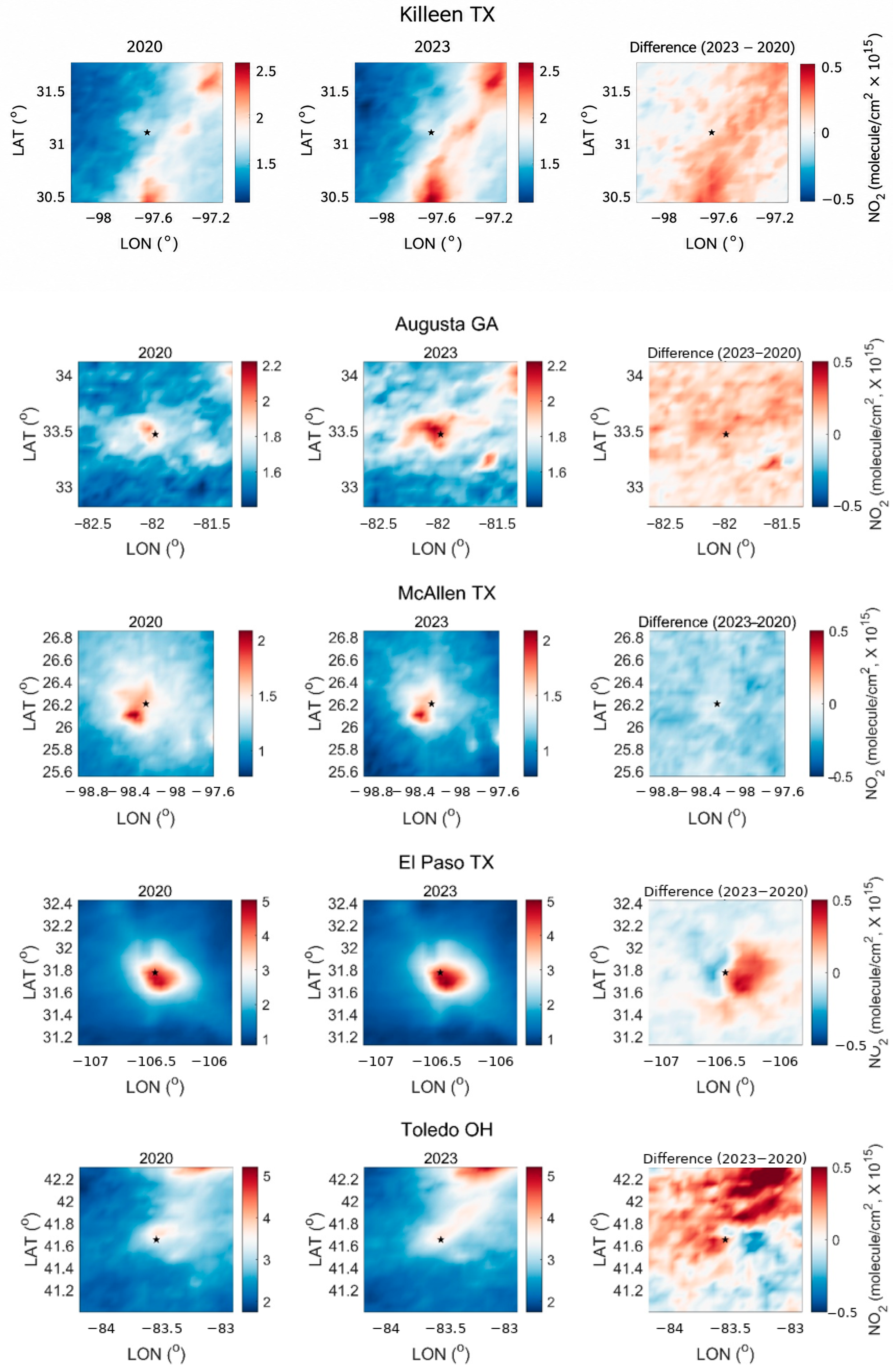
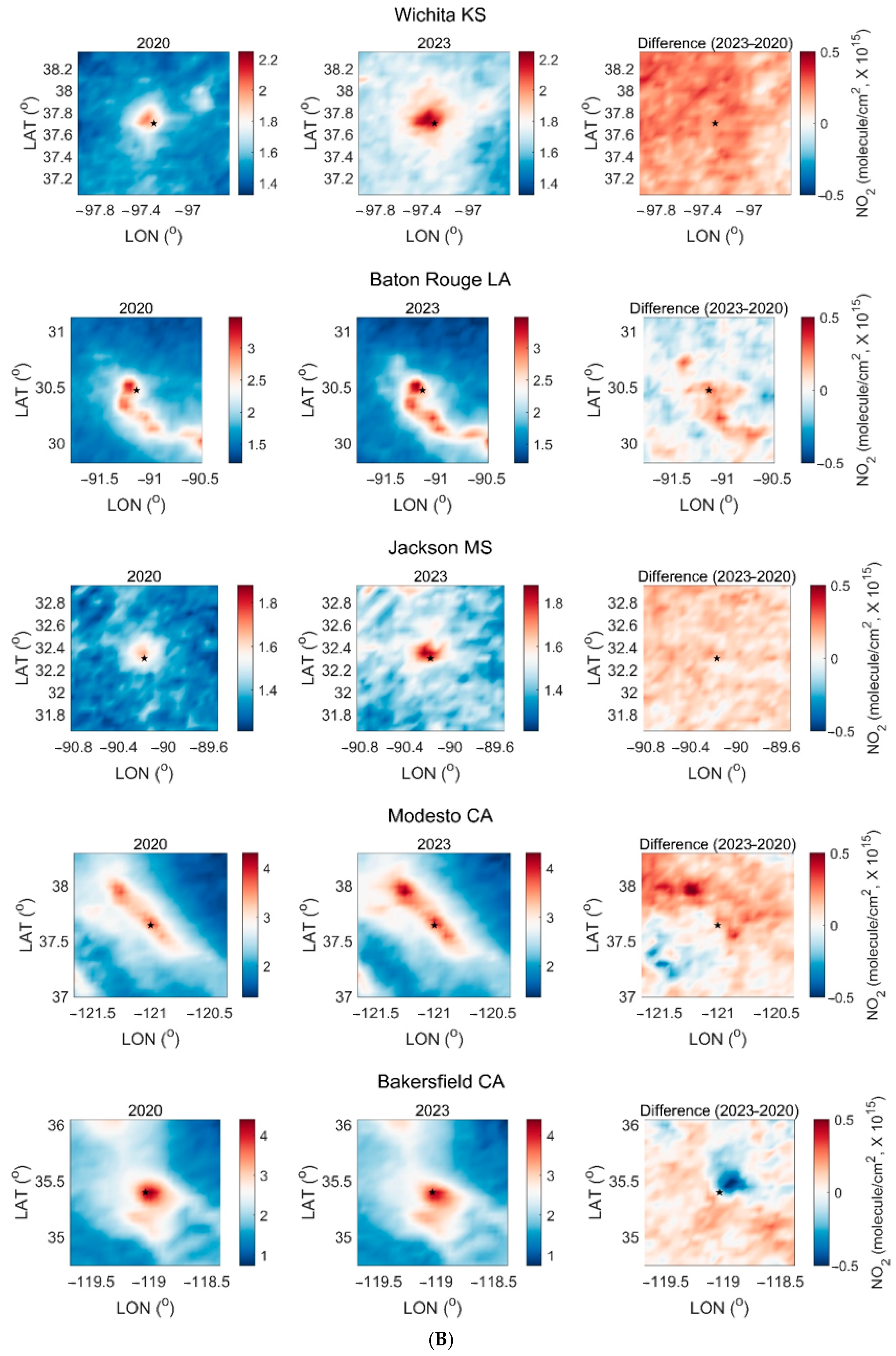

Disclaimer/Publisher’s Note: The statements, opinions and data contained in all publications are solely those of the individual author(s) and contributor(s) and not of MDPI and/or the editor(s). MDPI and/or the editor(s) disclaim responsibility for any injury to people or property resulting from any ideas, methods, instructions or products referred to in the content. |
© 2026 by the authors. Licensee MDPI, Basel, Switzerland. This article is an open access article distributed under the terms and conditions of the Creative Commons Attribution (CC BY) license.