


Abstract
Decoupling emissions from output is central to Saudi Arabia’s Vision 2030, yet the drivers of carbon intensity in oil-exporting economies—particularly how warming interacts with energy supply and income—remain poorly characterised. Using annual data for 1970–2023 and a country-specific Saudi temperature anomaly rather than a global proxy, we estimate the long-run drivers of carbon intensity in a cointegration framework addressing both a mean break in the cointegrating vector (identified endogenously by the Gregory–Hansen procedure at 2004) and a disturbance-variance break (1985). Headline estimates come from variance-weighted dynamic ordinary least squares, with the autoregressive distributed lag model and its nonlinear and quantile variants, fully modified ordinary least squares and canonical cointegrating regression providing dynamic, asymmetric, distributional and cross-estimator checks under Newey–West inference. Real GDP per capita lowers carbon intensity (β = −0.484) and industrial composition raises it (β = +0.449), while the temperature anomaly has a positive direct effect (β = +0.099). The two-way temperature–energy interaction is positive (+0.264) and the three-way temperature–energy–income interaction negative (−0.859): the marginal effect of +1 °C rises from +6.4% to +16.8% across the observed range of energy supply per capita but flattens as income rises. Because carbon intensity is CO2 divided by GDP, the negative income coefficient corresponds to a positive but sub-unitary elasticity of per capita emissions (+0.516), indicating relative rather than absolute decoupling. The estimates are conditional long-run associations, not identified causal effects.
1. Introduction
The Kingdom of Saudi Arabia occupies an unusual position in the global decarbonisation landscape. As one of the world’s largest oil exporters and the largest economy in the Middle East, it has historically pursued an energy-intensive industrialisation strategy financed by hydrocarbon rents. Since the announcement of Vision 2030 in 2016, the Kingdom has committed to a restructuring of its energy and economic systems, including a target of 50% renewable electricity generation by 2030 under the National Renewable Energy Programme [1,2] and net-zero greenhouse-gas emissions by 2060 under the Saudi Green Initiative [1]. Progress against the electricity target has so far been limited—independent assessments put the renewable share of generation at roughly 2% in 2024 [3]—which is precisely why the historical drivers of the country’s carbon intensity, the ratio of CO2 emissions to economic output, need to be understood before the credibility of forward-looking targets can be judged. Identifying which macroeconomic and energy levers most effectively decouple emissions from growth is a prerequisite for designing credible mitigation pathways. It is also, in a hot-climate economy, a problem of adaptation, because rising temperatures raise cooling-energy demand and therefore feed back into emissions, so that the same income and technology choices that mitigate emissions also shape the economy’s exposure to climate-induced energy stress.
Three features of the Saudi context make standard analyses of the income–energy–emissions relationship inadequate. First, the country experiences exceptionally high ambient temperatures and has the world’s highest share of air conditioning in household electricity consumption, at approximately 70% [4], making climate change itself a direct driver of energy use and, by extension, emissions. Second, the Saudi economy has shifted markedly across distinct policy regimes—from the pre-1986 OPEC reference-pricing era, through the post-1986 market-pricing regime, the 1995–2002 fiscal-consolidation period, the 2003–2014 oil-price super-cycle, and the post-2014 Vision 2030 reform programme—and structural breaks of this magnitude can render standard cointegration evidence misleading. Third, the temperature–energy–emissions relationship is plausibly heterogeneous across the conditional distribution of emission outcomes, with low- and high-emission regimes responding differently to identical income or energy shocks.
Research Gap and Contribution
Three gaps in the existing evidence motivate this study, and each maps onto a specific design choice.
First, a measurement gap. Studies that include a climate variable for Saudi Arabia almost invariably proxy local warming either with the global mean anomaly or with a short national record. Islam et al. [5], for example, use national temperature over the period of 1990–2019, but as a determinant of growth rather than of emissions intensity. The global anomaly is a poor instrument for the domestic cooling-demand channel because it is far smoother than the local series: over the period of 1970–2023, the Saudi country-mean anomaly used here ranges from −2.22 °C to +1.18 °C, a variation an order of magnitude larger than the corresponding global range. We therefore use a country-specific Saudi near-surface anomaly.
Second, a specification gap. The climate–energy–emissions literature has established that warming raises energy demand [6] and that the size of that response depends jointly on climate exposure and on income, because income governs air-conditioning penetration and equipment efficiency [7,8]. That conditional structure is almost never carried into single-country emissions models, which enter temperature additively. We embed the temperature anomaly as a direct regressor and as a moderator of the energy and income channels through two-way and three-way interaction terms, so that the income-dependence of the climate–emissions feedback becomes a testable restriction rather than an assumption.
Third, an inferential gap. Saudi time-series studies routinely acknowledge regime shifts but rarely test for a break in the cointegrating vector itself, and rarely distinguish a shift in the mean of that vector from a shift in its disturbance variance. Raggad [9] is an exception on the mean-break side, using impulse-saturation break tests. We identify the mean break endogenously by the Gregory–Hansen procedure, test separately whether it is a level, trend or slope shift, identify a disturbance-variance break, and estimate the long run by variance-weighted DOLS.
The contribution is therefore not the use of any single estimator, several of which are standard, but the combination: a country-specific climate measure, a conditional-marginal-effects specification that makes income-moderation testable, and an inferential design that separates mean from variance instability. We also report throughout what a 54-observation sample can and cannot support, and we are explicit that the estimates are conditional long-run associations rather than identified causal effects.
2. Literature Review
2.1. Income, Energy and Emissions in Saudi Arabia
The inverted-U relationship between income and pollution first proposed by Grossman and Krueger [10] and Selden and Song [11] has been documented across a wide range of economies, among them France [12], Central America [13] and the European Union [14]. The Saudi evidence base is larger than a summary of “Environmental Kuznets Curve studies generally find an inverted U” suggests, and it is more contradictory. Table 1 sets out the principal single-country studies, their samples, methods and findings; three patterns are worth drawing out.
The first is that the Environmental Kuznets Curve verdict for Saudi Arabia depends on the emissions measure. Working with aggregate CO2, Raggad [9] (1971–2014, ARDL with impulse-saturation breaks) rejects the Environmental Kuznets Curve outright: the GDP–pollution relation is positive in both the short and the long run. Alkhathlan [15] (1980–2008, ARDL/VECM) similarly finds the long-run income elasticity of emissions to exceed the short-run elasticity, implying that growth raises emissions over time. Moustafa et al. [16] (1970–2022, NARDL) again reject an inverted U. Working instead with carbon intensities disaggregated by emission source, Mahmood [17] (1968–2021) does substantiate an Environmental Kuznets Curve for gas and cement intensities. The apparent disagreement is largely definitional: because intensity divides emissions by GDP, an Environmental Kuznets Curve in intensity is a far weaker claim than one in emissions. This is the same accounting point that governs the interpretation of our own income coefficient (Section 5.7), and it is why Houaneb et al. [18] adopt per capita emissions as their primary outcome and treat carbon productivity only as a robustness check.
The second is that trade openness is genuinely contested in this literature rather than merely imprecisely estimated. Mahmood [17] reports that openness reduces the carbon intensities of oil, gas and cement emissions in the long run—the technique effect dominating. Alsubaie et al. [19] (1985–2023), by contrast, find that openness and foreign direct investment raise emissions, with geopolitical risk intensifying both. Moustafa et al. [16] also find openness emission-increasing. Our own estimates, reported below, are sign-consistent with the second group in the dynamic and semi-parametric estimators but not statistically distinguishable from zero in the DOLS-based specifications, and we treat openness accordingly as unresolved rather than as a finding.
The third is that the energy channel is the one point of agreement. Alshehry and Belloumi [20] (1971–2011), Raggad [9], Tlili et al. [21] (1970–2020) and Mohammed et al. [22] (1990–2023) all report large positive energy elasticities, with Tlili et al. estimating a long-run oil-driven growth elasticity of 1.34 and an asymmetric energy-shock effect of 1.87% against a 1.00% efficiency-gain effect. Mohammed et al. add that renewable deployment lowers the environmental footprint while industrial expansion raises it. Alajmi [23] reaches the same conclusion by log-mean Divisia index decomposition rather than regression. Where the literature is thin is on what conditions the size of that energy channel, which is the question this paper addresses.
2.2. Climate Feedbacks to Energy Demand
A second, largely separate literature quantifies the temperature–energy feedback. Auffhammer and Mansur [24] survey the early evidence; Wenz, Levermann and Auffhammer [25] show polarisation of European electricity load under warming; van Ruijven, De Cian and Sue Wing [6] project that vigorous warming raises global climate-exposed energy demand by 25–58% by mid-century. Two results in this literature are directly relevant to our specification. Romitti and Sue Wing [8] find that large temperature increases in tropical cities are partly offset by inelastic demand responses attributable to low air-conditioning penetration—that is, the temperature–electricity elasticity is itself a function of income. Colelli, Sue Wing and De Cian [7] make the mechanism explicit, showing that endogenous air-conditioning adoption creates a mitigation–adaptation trade-off whose magnitude differs sharply between affluent and poorer regions. For the Gulf specifically, Gurriaran et al. [26] estimate for Qatar a demand sensitivity of 1.7 GWh/°C, equivalent to 0.4 MtCO2/°C, and Howarth et al. [4] document that Saudi cooling-related electricity demand and its associated emissions plateaued after 2016 following efficiency standards, tariff reform and oil-to-gas switching in the power sector.
That last finding is important for the present paper because it is the closest thing in the literature to direct evidence on the mechanism our three-way interaction is designed to detect: a hot, high-income economy in which rising income coincided with a weakening of the temperature–emissions link. It is, however, descriptive and confined to 2010–2018. What has not been done is to test whether that moderation is present in the long-run cointegrating relationship over a five-decade sample, which is the gap this study fills.
2.3. Carbon Intensity Versus Absolute Emissions
Finally, the decoupling literature supplies the interpretive discipline this paper adopts. Haberl et al. [27], synthesising 835 empirical studies, find relative decoupling of GDP from CO2 to be common and absolute decoupling rare, and conclude that observed decoupling rates are far below those needed for stringent climate targets. Shuai et al. [28] formalise the ordering: economies decouple growth from carbon intensity first, from per capita emissions second, and from total emissions last, with 74%, 35% and 21% of 133 countries, respectively, having achieved each step by 2014. A declining carbon intensity is therefore the weakest of the three decoupling claims, and we are careful throughout not to present it as more.
Table 1.
Principal single-country empirical studies of Saudi emissions and carbon intensity.
Table 2.
Definitions of symbols, variables, parameters and abbreviations used in the paper.
3. Theoretical Framework and Derivation of the Empirical Model
The estimating equation is derived from an accounting identity rather than adopted by assumption. The derivation proceeds in three steps.
3.1. Step 1: From the Kaya Identity to a Carbon-Intensity Equation
Begin from the Kaya decomposition of aggregate emissions,
where P is population, Y is real output, and E is primary energy supply. Dividing both sides by Y and taking logarithms gives an exact identity for carbon intensity,
so that carbon intensity is the product of energy intensity and the carbon factor of the energy mix. Any determinant of carbon intensity must therefore operate through one or both of these two components. This is not a modelling assumption; it is arithmetic, and it disciplines the interpretation of every coefficient we report. It also implies the equivalent decomposition lnCI = lnCO2pc − lnGDPpc, which we exploit in Section 5.7.
CO2 = P × (Y/P) × (E/Y) × (CO2/E),
lnCI ≡ ln(CO2/Y) = ln(E/Y) + ln(CO2/E),
3.2. Step 2: Behavioural Determinants of the Two Components
Energy intensity E/Y falls with the capital stock’s efficiency and with a shift toward less energy-intensive activities, and rises with the share of heavy industry; it is therefore modelled as a function of real income per capita (a proxy for the vintage and efficiency of the capital stock) and of industrial composition. The carbon factor CO2/E is governed by the fuel mix, which in Saudi Arabia is dominated by oil and gas and moves slowly; it responds to income through the affordability of low-carbon substitutes and to trade openness through the technique and composition effects. Writing each component as a log-linear function of these drivers and substituting into (2) yields the additive core:
lnCIt = α + β1 lnGDPpct + β2 lnESPCt + β3 lnTOt + β4 lnIVAt + εt.
3.3. Step 3: The Climate Channel and the Conditional Specification
Equation (3) is silent on climate. In a hot economy, however, a temperature anomaly TA raises derived demand for cooling services. Let the additional energy required for cooling be ΔE(TA) and let its carbon content be that of the marginal generating unit. Two features of the Saudi system make the resulting effect on carbon intensity conditional rather than constant.
(i) The absolute quantity of climate-induced emissions scales with the size of the energy system, so the same anomaly has a larger effect on CI where energy supply per capita is higher. This delivers an interaction between TA and lnESPC. (ii) Income governs the substitution possibilities open to households and firms—high-efficiency and inverter air-conditioning, district cooling, demand-side management, electrified industrial heat—so the carbon content of the marginal cooling kilowatt-hour falls as income rises. This is precisely the income-dependence documented at the micro level by Colelli et al. [7] and Romitti and Sue Wing [8], and it delivers a three-way interaction between TA, lnESPC and lnGDPpc. Adding these terms to (3) gives the estimating equation
lnCIt = α + β1 lnGDPpct + β2 lnESPCt + β3 lnTOt + β4 lnIVAt + β5 TAt + β6 (TA·lnESPC)t + β7 (TA·lnESPC·lnGDPpc)t + εt.
Differentiating (4) with respect to TA gives the conditional marginal effect
where the subscript C denotes mean-centring. Two properties of (5) follow directly and are the reason the constituent variables are centred. First, β5 is not a “main effect” in any general sense: it is the marginal effect of temperature evaluated at the sample means of energy supply and income, and has no interpretation away from that point. Second, the standard error of (5) is not the standard error of β5; it involves the full covariance of (β5, β6, β7) and must be computed pointwise, which is why we report the marginal effect with confidence bands (Section 5.6), rather than reading significance off the interaction coefficients. Mean-centring leaves the highest-order coefficient β7 unchanged but makes the lower-order terms interpretable and removes the mechanical, non-essential collinearity between the products and their constituents [32,33].
∂lnCI/∂TA = β5 + β6 lnESPC_C + β7 (lnESPC_C⋯lnGDPpc_C),
Three hypotheses follow.
H1 (direct climate channel).
β5 > 0—a positive temperature anomaly raises carbon intensity, evaluated at the sample means of ESPC and GDPpc.
H2 (energy amplification).
β6 > 0—the climate–emissions channel is amplified at higher levels of energy supply, because more energy in a fossil-dominated mix means more emissions per unit of additional climate-induced demand.
H3 (income moderation).
β7 < 0—the joint climate–energy effect is attenuated at higher levels of GDP per capita. We label this moderation rather than “mitigation” deliberately: the design identifies whether the temperature–energy association is smaller at higher income, not whether income causes technological substitution. Testing the latter would require data on cooling-technology diffusion that we do not have (Section 6.2).
4. Materials and Methods
4.1. Nomenclature
All symbols, variables, parameters and abbreviations used in the paper are defined in Table 2.
4.2. Data
Annual time-series data for Saudi Arabia covering 1970–2023 (T = 54 observations) are assembled from international statistical sources. The dependent variable is the natural logarithm of carbon intensity (lnCI), measured as kilograms of CO2 emissions per constant 2015 US dollar of GDP. The provenance of this series warrants precision. It is constructed by the authors as the ratio of territorial (production-based) CO2 emissions to real GDP, with the emissions numerator taken from Our World in Data’s compilation of the Global Carbon Project and the GDP denominator from the World Bank World Development Indicators (WDI, constant 2015 US$). It is not downloaded as a pre-computed World Development Indicators or Our World in Data series. The constructed series was cross-checked against the Our World in Data published “kg CO2 per $ of GDP” series and against the discontinued World Development Indicators indicator EN.ATM.CO2E.PP.GD.KD, with no material divergence in the growth rates that identify the long-run relationship. The explanatory variables comprise four core regressors and a temperature anomaly: lnGDPpc (real GDP per capita in constant 2015 US$, WDI), lnESPC (total primary energy supply per capita in gigajoules per capita, Energy Institute), lnTO (trade openness, the sum of exports and imports as a share of GDP, WDI), lnIVA (industry value added as a share of GDP, WDI), and TA (a country-specific near-surface temperature anomaly for Saudi Arabia, in degrees Celsius). All four economic variables enter in natural-logarithmic form to permit elasticity interpretation; TA enters in level form because it can take negative values.
The temperature series. TA is the Berkeley Earth country-mean land-surface anomaly for Saudi Arabia. Berkeley Earth constructs gridded fields from the full archive of station records using a weighted least squares scheme with spatial kriging, which interpolates each station’s anomaly to arbitrary locations using an empirically estimated correlation-versus-distance function [34]; the land correlation scale is approximately 3300 km [35]. Because the method operates on anomalies rather than absolute temperatures and admits short and discontinuous records, stations need not span the full period and no gap-filling of individual station series is performed: grid cells with no nearby data receive proportionally wider uncertainty intervals rather than imputed values. The country series is the area-weighted average of the gridded field over the national land area. The 1951–1980 baseline is Berkeley Earth’s published reference climatology [34,35] and is retained here unchanged; because the baseline enters the anomaly as an additive constant over a fixed 30-year window, the choice shifts the level of TA but leaves its variance, its first differences and, hence, every estimated coefficient on TA in a mean-centred specification numerically unaffected. We verified this directly: re-centring TA on a 1961–1990 or 1991–2020 window changes only the intercept.
Data completeness. The compiled dataset contains no missing observations for any of the six primary series over the period of 1970–2023, and no observation was filled by interpolation, imputation or splicing. We confirmed this computationally by testing every series for the signature of linear interpolation—two or more consecutive identical first differences—and found no such run in any series (reported in Supplementary Table S6).
Two interaction terms are constructed to operationalise the conditional-marginal-effects framework: TESPC = TA_C × lnESPC_C and TESPCGDP = TA_C × lnESPC_C × lnGDPpc_C. All three of TA, lnESPC and lnGDPpc are mean-centred before the products are formed [32,33]. Table 3 summarises variable definitions, units, transformations and sources.
Table 3.
Variable definitions, units, transformations, and sources.
4.3. Empirical Strategy and the Role of Each Model
Because the paper deploys seven estimators, it is important to be explicit about which one supports which claim. The hierarchy is as follows, and Table 4 states it compactly.
Table 4.
Role of each model in the research design.
The autoregressive distributed lag (ARDL) bounds test establishes the existence of a long-run relationship; the Gregory–Hansen test verifies that this survives an endogenous break in the cointegrating vector. Neither is used to generate headline magnitudes. The conditional ARDL error-correction model is the dynamic representation: it supplies the speed of adjustment and the short-run dynamics, and its long-run solution is a cross-check. The variance-weighted dynamic ordinary least squares (DOLS) regression is the primary long-run specification and is the source of every headline magnitude reported in the Abstract, Section 5.5 and the Discussion; it is preferred because it absorbs regressor endogeneity parametrically through leads and lags rather than through a residual-based long-run-variance correction, and because it can be weighted to accommodate the 1985 disturbance-variance break. Fully modified ordinary least squares (FMOLS) and canonical cointegrating regression (CCR) are cross-estimator robustness checks on that specification. The nonlinear ARDL (NARDL) tests one specific auxiliary hypothesis—whether income and energy effects are asymmetric in sign of change—and is not used for headline magnitudes. The quantile ARDL (QARDL) is a descriptive check on whether the signs of the long-run coefficients are stable across the conditional distribution of carbon intensity; as Section 5.8 shows, its quantile-specific magnitudes are too imprecisely estimated in this sample to support inference, and none is drawn.
We also state plainly that applying several complex estimators to one small dataset is not by itself evidence of robustness, because they share the same data and may reproduce the same small-sample bias. Agreement across estimators is informative about specification sensitivity, not about sampling uncertainty. The checks that do speak to the latter are the sequential specification ladder (Section 5.4), the sample-cut comparison (Section 5.5), and the reporting of confidence intervals throughout.
The baseline long-run model to be tested is
where D2004t is identified endogenously by the Gregory–Hansen procedure and equals one from 2004 onward. The full pipeline is implemented in Python using statsmodels and arch. Estimation used Python 3.12 (Python Software Foundation, Wilmington, DE, USA) with statsmodels 0.14.6, arch 8.0.0, NumPy 2.x, pandas 2.x, SciPy 1.x, Matplotlib 3.x and openpyxl 3.1.5. Because residual diagnostics indicate serial correlation and heteroskedasticity (Section 5.9), all long-run and error-correction coefficients are reported with Newey–West heteroskedasticity- and autocorrelation-consistent (HAC) standard errors (Bartlett kernel, bandwidth 3). The compiled dataset and the complete estimation code are provided as the Supplementary Materials.
lnCIt = α0 + β1 lnGDPpct + β2 lnESPCt + β3 lnTOt + β4 lnIVAt + β5 TAt + β6 TESPCt + β7 TESPCGDPt + δ D2004t + εt
4.4. Unit-Root Testing
Three first-generation unit-root tests are applied to each series in level and first-differenced form: the Augmented Dickey–Fuller [36], the Phillips–Perron [37], and the Kwiatkowski–Phillips–Schmidt–Shin [38] tests. Augmented Dickey–Fuller lag lengths are selected using the Schwarz Bayesian information criterion; Phillips–Perron and Kwiatkowski–Phillips–Schmidt–Shin bandwidths use the Newey–West automatic procedure with a Bartlett kernel.
Conventional tests have low power against trend-stationary alternatives in the presence of structural breaks [39], so we additionally apply the Zivot–Andrews test [40] (Model C, one endogenous break, trimming λ ∈ [0.15, 0.85], lag length by the Schwarz Bayesian information criterion over k ∈ {0,…,4}) and the Lee–Strazicich [41] minimum-LM test with two endogenous breaks (Model C, trimming λj ∈ [0.10, 0.90], minimum two-period separation, lag length by the Schwarz Bayesian information criterion over k ∈ {0,1,2}).
Critical values for the Lee–Strazicich test. The tabulated critical values in Lee and Strazicich [41] are asymptotic and are commonly applied at T = 100. With T = 54, their use requires justification, which we now provide by simulation rather than assertion. We generated 2000 independent driftless random walks of length 54 and applied to each the identical two-break minimum-LM procedure—same trimming, same separation rule, same Schwarz Bayesian information criterion lag selection—recording the minimised LM t-statistic. The resulting finite-sample critical values are −5.863 (1%), −5.203 (5%) and −4.851 (10%). These are less negative than the −5.59 conventionally used at 5%, so applying the tabulated value in a T = 54 sample is conservative: it makes rejection of the unit-root null harder, not easier. We report inference against the simulated distribution and note where the two would differ. The simulated null distribution is provided with the replication code.
Both level and first-difference results are reported for the Lee–Strazicich test (Table 6), so that statements about the order of integration rest on evidence at both orders rather than on level results alone.
4.5. Cointegration and Long-Run Estimation
4.5.1. Autoregressive Distributed Lag (ARDL) Bounds Test
The bounds-testing procedure of Pesaran, Shin and Smith [42] is adopted in preference to the system-based approach of Johansen [43] because it is valid under a mixed I(0)/I(1) order of integration provided no series is I(2), has good small-sample properties in T ≈ 50 settings [44], and yields consistent long-run estimators under regressor endogeneity. The unrestricted error-correction representation of (6) is
where Xk indexes the seven explanatory variables and lag lengths are selected by the Akaike information criterion over a maximum of two lags. Long-run elasticities are recovered as βi = −θi/θ0 with delta-method standard errors. One distinction deserves emphasis: because D2004 enters (7) undifferenced and contemporaneously, its estimated coefficient δ is a short-run impact effect, while the corresponding long-run level shift is −δ/θ0. The two are reported separately (Table 8).
ΔlnCIt = α0 + Σi φi ΔlnCIt−i + Σk Σj ψkj ΔXk,t−j + θ0lnCIt−1 + Σk θk Xk,t−1+ δ D2004t + εt
4.5.2. Gregory–Hansen Cointegration Test with Structural Break
We apply the Gregory and Hansen [45] procedure, which permits a single endogenous regime shift in the cointegrating vector under the alternative. Three variants are estimated: Model C (level shift), Model C/T (level shift with trend) and Model C/S (regime shift in intercept and slopes). For each candidate break date τ ∈ [0.15T, 0.85T], the residuals from the cointegrating regression are tested for a unit root by an Augmented Dickey–Fuller regression; the statistic is the most negative ADF* across τ. Two specifications are tested: Specification 1 with the four core regressors (m = 4) and Specification 2 with the temperature-augmented set (m = 5). Critical values are from Gregory and Hansen [45].
We now supplement this with a direct test of the form of the break, since a residual-based test that rejects most strongly under Model C/S does not by itself establish that slopes shifted: the three variants have different critical values and are not nested comparisons. We therefore re-estimate the long-run relationship with (i) a level dummy, (ii) a level dummy plus a post-break trend, and (iii) a level dummy plus interactions between the dummy and lnGDPpc, lnESPC and TA, and test the added terms by Wald statistics (Table 7, Panel C).
4.5.3. Nonlinear ARDL (NARDL): Asymmetric Long-Run Dynamics
To relax the symmetry assumption, we estimate the nonlinear ARDL of Shin, Yu and Greenwood-Nimmo [46], decomposing lnESPC and lnGDPpc into partial-sum processes
Xt+ = Σh max(ΔXh, 0), Xt− = Σh min(ΔXh, 0)
Long-run asymmetry is tested by the Wald restriction β+ = β−. D2004 is retained as an exogenous regressor.
4.5.4. Quantile ARDL (QARDL): Distribution-Conditional Dynamics
We estimate the quantile ARDL of Cho, Kim and Shin [47] at τ ∈ {0.25, 0.50, 0.75}:
Q_{ΔlnCI}(τ | Ωt−1) = α(τ) + Σi φi(τ) ΔlnCIt−i + Σk Σj ψkj(τ) ΔXk,t−j + ρ(τ) ECTt−1
Estimation is by linear-programming quantile regression [48]. Inference requires care in this sample and we now report it explicitly. Every quantile regression uses all n = 53 usable observations with k = 17 parameters (residual degrees of freedom 36); what differs across quantiles is the weighting, not the sample size, and we report the number of observations lying below and above each fitted quantile plane as the relevant measure of effective information. Because the long-run coefficients are ratios −θk(τ)/θ0(τ), their sampling distribution is skewed and heavy-tailed, and delta-method standard errors are unreliable. We therefore report percentile confidence intervals from 1000 paired (xy-pair) bootstrap resamples, drawn with replacement and re-estimating the full quantile regression in each replication (seed 20260825). Coefficient signs alone are not treated as evidence.
4.5.5. Cointegrating-Regression Estimators and the Treatment of Deterministic Terms
Three single-equation cointegration estimators are applied: fully modified ordinary least squares [49], dynamic ordinary least squares [50] and canonical cointegrating regression [51]. FMOLS applies a non-parametric correction for serial correlation and endogeneity; DOLS augments the cointegrating regression with leads and lags of the differenced regressors; CCR transforms the regressors to remove second-order bias. The DOLS lead–lag order is one lead and one lag.
Treatment of the deterministic break term. The break dummy requires a treatment distinct from that given to the stochastic regressors, and the distinction has material consequences. Applying the lead–lag augmentation, and the long-run covariance corrections, to all columns of the regressor matrix, including the deterministic step dummy D2004, would be a specification error. Differencing a step dummy produces an impulse dummy, so such an augmentation inserts impulse dummies at 2003, 2004 and 2005, absorbing precisely the observations that identify the level shift and inflating the estimated δ. D2004 is a deterministic component, not a stochastic I(1) regressor: it enters the cointegrating regression alongside the constant, but is excluded from the differenced regressor set used to construct the lead–lag augmentation and the corrections Ω and Λ. All FMOLS, DOLS, CCR and variance-weighted DOLS results reported below adopt this treatment. It leaves the substantive coefficients almost unchanged but matters materially for δ, and Section 5.2 quantifies the difference.
4.5.6. Choice of the Structural-Break Dummy
The choice of break date rests on three grounds. Statistically, Gregory–Hansen Model C/T endogenously identifies 2004 under both Specification 1 (m = 4; ADF* = −6.534) and Specification 2 (m = 5; ADF* = −6.910), both rejecting no-cointegration at 1%. These two specifications are not independent of one another: they share the same dependent variable and four of five regressors, so their agreement establishes only that adding TA does not displace the break date. Methodologically, Model C/T is the counterpart to the Zivot–Andrews Model C used in unit-root testing. Economically, 2004 marks the onset of the 2003–2008 oil-price super-cycle. Documented developments over that window include the expansion of Saudi Aramco and SABIC capital-investment programmes, the launch of the Economic Cities programme, substantial additions to installed generation capacity, and growth in thermal desalination capacity; these are set out in the assessments of Saudi climate and energy policy by Al Shehri et al. [52] and Howarth et al. [4], and in Alajmi’s decomposition of Saudi emissions drivers [23]. The dummy is included in all specifications as an exogenous regressor, and the ARDL is re-estimated with D1986, D2008 and D2014 alternatives (Supplementary Table S3).
4.5.7. Variance Break and Robust Estimation
Saudi macroeconomic series exhibit not only shifts in mean dynamics but a pronounced change in volatility. A variance-ratio test on the error-correction residuals locates a break in 1985 (pre- versus post-1985 residual-variance ratio F = 5.32, p < 0.001), coinciding with the 1986 oil-price collapse. Conditional heteroskedasticity does not bias the cointegrating estimates but renders equally weighted estimation inefficient. We therefore (i) adopt DOLS as the primary long-run estimator, (ii) estimate it by feasible generalised least squares, weighting observations by the inverse of their regime-specific variance, and (iii) report Newey–West HAC standard errors throughout. The long-run model is also re-estimated on the post-1985 subsample.
4.6. Diagnostic and Stability Tests
Post-estimation diagnostics comprise the Breusch–Godfrey serial-correlation LM test [53], the Breusch–Pagan–Godfrey heteroskedasticity test, the ARCH-LM test of order 2, the Jarque–Bera normality test [54], the Ramsey RESET test [55] and variance inflation factors. Parameter stability is assessed by cumulative sum (CUSUM) and cumulative-sum-of-squares plots of recursive residuals [56]. Test statistics as well as p-values are reported (Table 15), and collinearity is assessed with the correlation matrix, Belsley scaled condition indices and drop-variable re-estimation in addition to the variance inflation factors (see the Collinearity Section).
5. Results
5.1. Stationarity and Structural Breaks
Figure 1 plots the six primary series. Table 5 reports the conventional unit-root tests. Variable definitions and sources are given in Section 4.2 and are not repeated here.
Figure 1.
Key variables, Saudi Arabia, 1970–2023. The dotted vertical line marks the 2004 endogenous structural break. Panel (d) shows the country-specific Saudi temperature anomaly, whose interannual variability is substantially greater than that of a global anomaly.
Table 5.
Conventional unit-root tests (ADF, Phillips–Perron, KPSS).
Table 6 reports the structural-break unit-root tests. Panel A gives the Zivot–Andrews test; Panel B now reports the Lee–Strazicich test in both levels and first differences, evaluated against the simulated T = 54 critical values derived in Section 4.4.
Table 6.
Unit-root tests with endogenous structural breaks. Panel A. Zivot–Andrews test (Model C, one endogenous break). Panel B. Lee–Strazicich test (Model C, two endogenous breaks), levels and first differences.
Three observations follow. First, no variable is I(2): first-difference rejection occurs at 1% or 5% for every series across all tests, satisfying the bounds-testing prerequisite of Pesaran et al. [42]. Because the Lee–Strazicich test is reported at both orders, this conclusion does not rest on Augmented Dickey–Fuller and Phillips–Perron evidence alone: the two-break LM test rejects the unit-root null in first differences for every series at the 1% level (p ≤ 0.003), while failing to reject in levels for all four macroeconomic series. Second, the country-specific temperature anomaly is I(0)—stationary in levels under the Augmented Dickey–Fuller, Phillips–Perron, Kwiatkowski–Phillips–Schmidt–Shin, Zivot–Andrews and Lee–Strazicich tests—while lnCI, lnGDPpc, lnTO and lnIVA are I(1) and lnESPC is borderline. This mixed I(0)/I(1) configuration with no I(2) series is the setting for which the ARDL bounds framework is designed. Third, the endogenously identified break dates cluster in three substantively meaningful periods: 1975–1989 (the second oil-price boom and the 1986 collapse), 2003–2008 (the super-cycle and global financial crisis), and 2014–2018.
5.2. Cointegration and the Form of the 2004 Break
Table 7 reports the cointegration evidence. The ARDL bounds F-statistic of 5.042 exceeds the Pesaran et al. [42] 1% upper bound of 4.09 (k = 7, Case III); the t-statistic on the lagged level of the dependent variable is −5.65, also consistent with cointegration. The Gregory–Hansen test rejects the no-cointegration null at 1% under all six model-specification combinations, and Model C/T identifies 2004 under both the core (m = 4) and temperature-augmented (m = 5) specifications.
Table 7.
Cointegration tests and the form of the structural break. Panel A: ARDL bounds test (k = 7 regressors plus D2004; Case III). Panel B: Gregory–Hansen test with endogenous break in the cointegrating vector. Panel C: Direct tests of the form of the 2004 break (variance-weighted DOLS).
Panel C settles the form of the break. It is tempting to infer from the fact that Gregory–Hansen Model C/S produces the most negative ADF* that the cointegrating relationship experienced a slope shift as well as a level shift, but that inference does not follow: the three variants have different critical values and are not a nested sequence, so their statistics cannot be ranked against one another. Tested directly, the level shift is strongly supported, the post-break trend shift is not (p = 0.144), and the joint restriction that the slopes on lnGDPpc, lnESPC and TA are unchanged after 2004 cannot be rejected (χ2 = 5.997, p = 0.112). We therefore characterise 2004 as a level shift in the cointegrating vector. Substantively, this is a modest reading: the elasticities of carbon intensity with respect to its determinants did not detectably change after 2004; what changed was the level around which the relationship holds.
The last row of Panel C is reported for transparency. The level-shift coefficient is the one parameter in this model that is not robust across estimators: it is −0.103 in variance-weighted DOLS, −0.087 in unweighted DOLS, −0.180 in FMOLS, −0.105 in CCR, −0.066 and insignificant in the ARDL long-run solution, and +0.006 and insignificant in a static ordinary least squares cointegrating regression with no endogeneity correction at all. We do not attempt to adjudicate among these. The economically meaningful statement is the one that survives all of them: conditional on the seven regressors, the post-2004 regime does not exhibit a large residual level shift in carbon intensity, because the break is largely absorbed by the changing levels of the explanatory variables themselves. None of the substantive coefficients depends on which treatment of the dummy is adopted (Table 10).
The break date should be read as the inflexion point of a multi-year structural transition rather than a single-year event: a break in the cointegrating vector reflects the cumulative reconfiguration of the economy’s energy–output relationship, which materialised with a lag relative to the 2003 onset of the price upswing.
5.3. ARDL Long-Run and Short-Run Dynamics
Table 8 reports the ARDL long-run elasticities and the error-correction representation. The model is estimated in conditional error-correction form over 53 observations (1971–2023) with one lag per variable and Newey–West HAC standard errors; long-run coefficients are recovered as βi = −θi/θ0 with delta-method standard errors. Confidence intervals are reported alongside p-values because, with 53 observations and 17 parameters, the width of the interval is at least as informative as the location of the point estimate.
Table 8.
ARDL long-run and error-correction estimates. Panel A. Long-run elasticities (dependent variable: lnCI). Panel B. Error-correction representation and model dimensions.
The long-run coefficient on lnGDPpc is −0.562 (t = −13.20); the coefficients on lnTO (+0.272) and lnIVA (+0.317) are positive and significant at 5%, and the energy-supply level effect is small and insignificant, with its influence operating through the temperature interactions. The temperature anomaly shows a positive direct effect (β5 = +0.087, p < 0.001); the two-way interaction is positive (β6 = +0.523, p = 0.013) and the three-way interaction is negative (β7 = −1.515, p = 0.006); the pattern is predicted by H1–H3. The error-correction coefficient is −0.607: approximately 61% of any short-run deviation from long-run equilibrium is corrected within one year. An adjusted R2 of 0.468 in a differenced specification is unremarkable—the dependent variable is ΔlnCI, not lnCI—but it does confirm that a substantial share of annual variation in the change in carbon intensity is unexplained, and we do not claim otherwise.
5.4. Sequential Specification and Model Dimensions
The baseline model estimates 17 parameters from 53 observations, which raises the question whether the interaction terms are identified or merely fitted. Table 9 addresses this by introducing the regressors sequentially rather than simultaneously, reporting for each step the parameter count, residual degrees of freedom and information criteria, and Figure 2 plots the resulting coefficient paths with confidence intervals.
Table 9.
Sequential specification ladder: long-run coefficients, model dimensions and information criteria.
Figure 2.
Stability of the long-run coefficients on income, temperature and the three-way interaction as regressors and interactions are introduced sequentially (M1–M5), with 95% confidence intervals.
Three points follow. First, the two coefficients that carry the paper’s substantive claims are stable as the specification is built up: the income elasticity stays within −0.47 to −0.56 across all five models, and the direct temperature effect stays within +0.069 to +0.109 across the four in which it appears. Neither is an artefact of the interaction terms. Second, the added parameters pay for themselves by parsimonious criteria: the Schwarz Bayesian information criterion (BIC), which penalises parameters most heavily, improves from −109.61 at M3 to −118.39 at M4 when the three-way interaction is added, so that term improves fit by more than its two additional parameters cost. This is the relevant answer to the over-parameterisation concern—not that the model is small, but that the terms in question earn their place. Third, BIC is minimised at M4, without the break dummy (−118.39 versus −115.65 at M5). We retain D2004 because it is endogenously identified and because the Gregory–Hansen evidence for a break in the cointegrating vector is strong, but a purely information-theoretic criterion would drop it, which is consistent with the finding in Section 5.2 that the dummy is largely absorbed by the regressors.
Note also that the sign of the two-way interaction TESPC changes between M3 (−0.052, insignificant) and M4 (+0.449). This is expected rather than anomalous: in M3 the two-way term is constrained to be constant across income levels, so it estimates an average over a relationship that in fact varies with income. Interpreting a lower-order interaction in the absence of the higher-order term it belongs to is a known specification error [33], and the M3 estimate should not be read as evidence against H2.
5.5. Primary Long-Run Estimates
Table 10 reports the primary specification—variance-weighted DOLS with the break dummy treated as a deterministic term—alongside unweighted DOLS, FMOLS, CCR and a post-1985 subsample.
Table 10.
Long-run estimates: primary specification and cross-estimator comparison.
Figure 3 compares the long-run coefficient estimates across the six estimators. Three features are decisive. First, the income elasticity is effectively invariant across the four full-sample estimators (−0.475 to −0.484) and the direct temperature effect is positive and significant in every one, though its magnitude ranges more widely (+0.095 to +0.182), with FMOLS and CCR producing the larger values. Second, the three-way interaction is negative in every column, significantly so under both DOLS variants but not under FMOLS or CCR, whose point estimates are roughly half the size with standard errors of comparable magnitude. The estimators should not therefore be described as converging on a magnitude: the sign is robust, the magnitude is not tightly pinned down, and the data support the direction of income moderation more strongly than its size. Third, trade openness is not robust. It is positive and significant in the dynamic ARDL and in FMOLS and CCR, indistinguishable from zero in both DOLS columns, and significantly negative on the post-1985 subsample. Given that the Saudi literature is itself split on this coefficient [17,19], we treat openness as unresolved rather than as a finding.
Figure 3.
Long-run coefficient estimates across estimators with 95% confidence intervals (NARDL lnGDPpc shown as the positive partial sum).
The post-1985 column deserves a specific caveat. With 36 observations and 30 parameters, it retains only 6 residual degrees of freedom, and its coefficients on lnESPC, TESPC and TESPCGDP move sharply. It is included because it tests whether the results are driven by the high-variance early period, and for the two headline coefficients the answer is no: income remains strongly negative and temperature strongly positive. The subsample magnitudes are not interpreted, and the intervals in Figure 4 show why.
Figure 4.
Stability of the headline DOLS long-run coefficients across sample cuts (variance-weighted, full sample, post-1985), with 95% confidence intervals.
5.6. Conditional Marginal Effects of Temperature
Because the meaning of interaction coefficients depends on centring and specification, the substantive result is the conditional marginal effect of Equation (5), not the individual βs. Table 11 evaluates it on a grid of energy-supply and income values with standard errors computed from the full covariance matrix, and Figure 5 plots it continuously with 95% bands.
Table 11.
Conditional marginal effect of a +1 °C temperature anomaly on carbon intensity.
Figure 5.
Conditional marginal effect of a +1 °C temperature anomaly on carbon intensity as a function of energy supply per capita, evaluated at three income levels, with 95% confidence bands.
The gradient is the result. Holding income at its mean, the marginal effect of +1 °C rises from +6.4% at one standard deviation below the mean energy supply to +13.3% at one standard deviation above and +16.8% at two, and the confidence interval excludes zero throughout most of the observed range. Holding energy supply at the top of its range instead and varying income, the same effect falls from +24.9% at low income to +8.7% at high income. This is the income-moderation result stated in the units that matter, and it is visible in Figure 5 as the progressive flattening of the slope as income rises. It is also, as Figure 5 makes clear, estimated with wide uncertainty in the corners of the grid where few observations lie: at one standard deviation below mean energy supply and one below mean income, the effect is not distinguishable from zero.
5.7. Alternative Dependent Variables and the Meaning of the Income Coefficient
Carbon intensity is CO2 divided by GDP, and lnGDPpc appears on the right-hand side. The strong negative income coefficient may therefore be in part an accounting consequence rather than evidence of decarbonisation, and this deserves to be stated precisely. From the identity lnCI = lnCO2pc − lnGDPpc, any regression of lnCI on lnGDPpc and controls has an exact counterpart in which lnCO2pc is the dependent variable and the income coefficient is larger by exactly one; all other coefficients are numerically identical. Table 12 reports the three exactly related re-expressions, and the identity holds to four decimal places in our estimates.
Table 12.
Alternative dependent variables (variance-weighted DOLS).
Three conclusions follow. First, the elasticity of per capita emissions with respect to income is +0.516, positive and strongly significant. Saudi emissions per head rise with income; they simply rise more slowly than income does. In the taxonomy of Shuai et al. [28], this is the first and weakest of the three decoupling steps—decoupling of growth from carbon intensity—and it is entirely consistent with rising absolute emissions. Second, it follows that the negative coefficient should not be read as evidence of the descending portion of an Environmental Kuznets Curve. A sub-unitary positive elasticity of emissions with respect to income is not the descending limb of an Environmental Kuznets Curve; it is the ordinary case, and it is what Raggad [9] and Alkhathlan [15] report for Saudi Arabia using emissions rather than intensity as the dependent variable. Our results are therefore not in conflict with theirs; they are the same finding expressed in a different denominator. Third, and reassuringly for the paper’s central argument, the temperature and interaction coefficients are numerically invariant to which of these three measures is used, because the re-expression touches only the income and energy terms. The climate–energy–income result does not depend on the choice of carbon intensity as the outcome.
The fourth column decomposes the outcome along the other axis of the Kaya identity. With energy intensity E/GDP as the dependent variable and lnESPC removed from the regressor set, the income coefficient is −1.093 and the direct temperature effect is small, negative and insignificant (−0.018), while both interaction terms are large and significant (TESPC +0.474, TESPCGDP −1.478). The reading is instructive: at the sample means of energy supply and income, temperature has no detectable effect on energy intensity, and the direct climate effect on carbon intensity therefore operates mainly through the carbon factor. The conditional climate channel, by contrast, runs strongly through energy intensity, which is what the mechanism in Section 3.3 predicts: additional cooling load raises energy use per unit of output more where the energy system is already large, and less where income permits efficient equipment.
We take total emissions no further than this. Converting per capita to total emissions requires only the addition of ln population, and Saudi population grew several-fold over a period of 1970–2023, so total territorial emissions rose over the period on any reading. Nothing in this paper should be taken as evidence of falling Saudi emissions.
5.8. Asymmetric and Distribution-Conditional Evidence
Table 13 reports the NARDL estimates. The bounds F-statistic is 10.04 and the error-correction coefficient is −0.613, closely matching the symmetric ARDL. The partial-sum decomposition of lnGDPpc is asymmetric: the positive partial sum is −0.764 (p < 0.001) while the negative partial sum is −0.261 and insignificant, with the Wald test of long-run symmetry rejected at 10% (χ2 = 2.902, p = 0.089); symmetry of the lnESPC partial sums is rejected at 5% (χ2 = 5.232, p = 0.022). The direct temperature effect remains positive and highly significant (+0.080). The three-way interaction retains its negative sign (−0.656) but is not significant (p = 0.234): the decomposition adds four parameters to a 53-observation sample and the term is estimated far less precisely. We read the NARDL as confirming the direction of the income-moderation effect under a more demanding parameterisation, and we do not draw a magnitude from it.
Table 13.
NARDL long-run asymmetric estimates.
Table 14 reports the QARDL estimates with bootstrap confidence intervals, and inference here requires particular care. With 1000 paired bootstrap resamples, the estimates prove far less precise than the point estimates alone would suggest: the long-run coefficients are ratios estimated from 53 observations with 17 parameters, and their bootstrap intervals are wide. Only the income elasticity is distinguishable from zero, and only at τ = 0.25 (p = 0.048) and marginally at τ = 0.50 and τ = 0.75. Every other coefficient, including the three-way interaction, has an interval spanning zero at all three quantiles.
Table 14.
QARDL long-run estimates with 95% bootstrap confidence intervals.
We therefore restrict the QARDL claim to what the evidence supports: the point estimates are sign-consistent with the mean-based results—income negative at all three quantiles, temperature positive at all three, the three-way interaction negative at all three—but the sampling uncertainty at any individual quantile is too large in a 53-observation sample to support statements about quantile-specific magnitudes or about heterogeneity across the distribution. In particular, the data support neither a claim that the coefficients are significant at the tails, nor the policy inference that mitigation effects would be similar across emission regimes. Figure 6 plots the long-run coefficients and their bootstrap intervals across the three quantiles.
Figure 6.
QARDL long-run coefficients across the conditional distribution of carbon intensity with 95% bootstrap confidence intervals.
5.9. Diagnostics, Parameter Stability and Collinearity
Table 15 reports the post-estimation diagnostics with test statistics as well as p-values, and states the consequence of each result for inference.
Table 15.
Post-estimation diagnostics for the conditional error-correction model.
The consequences are as follows. Residual autocorrelation at orders two and four and heteroskedasticity are present at the 5% level. Neither biases the cointegrating estimates, which are super-consistent, but both render OLS standard errors inconsistent, which is precisely why every coefficient in this paper is reported with Newey–West HAC standard errors rather than ordinary least squares ones. The effect is not cosmetic: for the lagged level of TA, the HAC standard error is 0.0195 against an ordinary least squares value of 0.0272, moving the p-value from 0.059 to 0.007; for the three-way interaction it is 0.323 against 0.398, moving the p-value from 0.027 to 0.004. In both cases, HAC correction strengthens the result, so the departures from the classical assumptions are not what is generating significance. The correct functional form is not rejected at 5% by RESET at either power, although the power-3 statistic is borderline (p = 0.055), which we note as a caution against reading the log-linear specification as exact. The ARCH statistic is at the 5% boundary; combined with the variance-ratio test, this is the evidence motivating the variance-weighted estimation of Section 4.5.7, rather than a nuisance to be reported and set aside.
Parameter stability is shown in Figure 7. The CUSUM statistic remains within the 5% bands throughout, confirming stability of the conditional-mean relationship. The CUSUM-of-squares moves outside the bands during the early-to-mid 1980s before returning, signalling a break in the disturbance variance rather than in the coefficients, consistent with the 1985 variance break.
Figure 7.
CUSUM and CUSUM-of-squares parameter-stability tests for the error-correction model.
Collinearity
Variance inflation factors are sensitive to whether the auxiliary regression includes an intercept, and in a model whose regressors are logarithms of variables with large means that sensitivity is extreme. Auxiliary regressions of each regressor on the remaining six, estimated without an intercept, return variance inflation factors of approximately 1859 for lnGDPpc, 1472 for lnESPC, 1542 for lnTO and 1443 for lnIVA. These figures are artefacts of scaling rather than properties of the data: lnGDPpc has a mean of 10.28 and a standard deviation of 0.356, so an auxiliary regression without a constant must explain the mean as well as the variation, driving the auxiliary R2 arbitrarily close to one. Computed with an intercept, the maximum variance inflation factor in the model is 9.75. Table 16 reports both, together with correlation and condition-index diagnostics.
Table 16.
Collinearity diagnostics.
The condition-index evidence tells the same story. On the raw scaled design including the intercept, the condition number is 465, which would ordinarily be alarming. After mean-centring the regressors, it falls to 8.7, far below the conventional threshold of 30. The difference is entirely attributable to the near-constant columns created by logging variables with large means; it is a scaling phenomenon, not an identification failure, and mean-centring—which we perform for the interaction constituents in any case—removes it. The largest pairwise correlation among the regressors is 0.872, between lnESPC and the three-way interaction.
A further question is whether the interaction coefficients remain stable when the composition variables are omitted. They do in sign but not in precision. Dropping lnIVA gives lnGDPpc −0.528, TA +0.139, TESPC +0.530 and TESPCGDP −1.222; dropping lnTO gives −0.481, +0.086, +0.167 and −0.713; dropping both gives −0.549, +0.053, +0.431 and −0.817. The income elasticity is stable throughout. The three-way interaction is negative in every subset but loses significance when lnTO is removed. We do not read this as collinearity-induced instability, because the correlation between lnTO and the interaction terms is modest (0.093 and 0.401); the more likely explanation is omitted-variable bias from dropping a composition control that belongs in the model. The full-model estimates are therefore the ones we report.
5.10. Robustness to Alternative Break Dates
Supplementary Table S3 reports the ARDL results under D1986, D2008 and D2014 in place of D2004. Because the dummy enters as a fixed regressor, the bounds F-statistic is invariant at 5.042. Across all four specifications, the error-correction coefficient is negative and significant (−0.607 to −0.581), and the elasticities retain their signs and approximate magnitudes: lnGDPpc between −0.476 and −0.562, TA between +0.059 and +0.087, TESPC between +0.333 and +0.523, and TESPCGDP between −1.515 and −1.764. The choice of break date does not alter any substantive conclusion.
6. Discussion
6.1. What the Estimates Show
The principal empirical result is the contrast between a positive two-way temperature–energy interaction and a negative three-way temperature–energy–income interaction in the long-run determination of Saudi carbon intensity. Expressed as conditional marginal effects rather than as coefficients, a +1 °C anomaly raises carbon intensity by about 9.9% at the sample means of energy supply and income; by about 13.3% at one standard deviation above mean energy supply; and by about 8.7% when energy supply is two standard deviations above its mean but income is one standard deviation above as well. The temperature–carbon relationship is thus not a constant elasticity but a surface whose slope depends on where the economy sits in energy–income space.
6.2. Interpreting the Mechanism, and Its Limits
The natural economic reading is that in a fossil-dominated supply mix additional cooling demand translates into proportionally more emissions per unit of energy, and that higher income permits substitution toward less carbon-intensive cooling (high-efficiency and inverter air-conditioning, district cooling, demand-side management), transport and industrial process heat. This reading is consistent with the micro evidence: Colelli et al. [7] show that air-conditioning adoption and its emissions consequences differ sharply between affluent and poorer regions; Romitti and Sue Wing [8] attribute the inelastic temperature response of tropical cities to low air-conditioning penetration; and Howarth et al. [4] document that Saudi cooling-related electricity demand and its emissions plateaued after 2016 following efficiency standards, tariff reform and oil-to-gas switching.
We must nonetheless be explicit about what this design does and does not identify. The model contains annual temperature anomaly, primary energy supply and GDP per capita. It does not contain cooling electricity demand, air-conditioning stock or efficiency, peak load, building-envelope performance, or the renewable share of generation. It therefore cannot observe the technological substitution channel; it can only establish that the temperature–carbon-intensity association is smaller at higher income, conditional on the other regressors. The correct description of β7 < 0 is a conditional long-run association, not a validated causal mechanism, and we accordingly use the term income moderation rather than income mitigation throughout and do not present the technology channel as demonstrated. A direct test would require a specification in which cooling demand, appliance efficiency and generation mix enter as observed process variables; assembling such a series for Saudi Arabia over five decades is the most valuable extension of this work.
Two further considerations counsel restraint. First, the broader literature is not unanimous that income reduces carbon outcomes: consumption-based accounting frequently shows scale effects outweighing efficiency gains, so our result should be read as specific to the production-based measure and to Saudi Arabia. Second, the magnitude of β7 is not tightly identified. It is negative under all six estimators but significant under only three of them, and its confidence interval under the primary specification runs from −1.68 to −0.04. The direction is robust; the size is not.
6.3. Income, Trade and Composition
The income result requires the framing established in Section 5.7. The long-run elasticity of carbon intensity with respect to income is −0.484; the elasticity of per capita emissions with respect to income is +0.516. Saudi growth has been accompanied by relative decoupling only. Placed in the taxonomy of Shuai et al. [28], Saudi Arabia has taken the first of three decoupling steps, and Haberl et al. [27] make clear that this is the common case internationally and falls far short of what stringent climate targets require. The negative coefficient does not evidence the descending limb of an Environmental Kuznets Curve, and our finding is in fact consistent with, rather than contrary to, the studies that reject the Environmental Kuznets Curve for Saudi Arabia using emissions as the dependent variable [9,15,16].
On trade openness, we report a non-result. The coefficient is positive and significant in the ARDL, FMOLS and CCR, indistinguishable from zero in both DOLS specifications, and negative on the post-1985 subsample. This estimator-dependence mirrors an unresolved disagreement in the Saudi literature, where Mahmood [17] finds openness reduces source-specific carbon intensities, while Alsubaie et al. [19] and Moustafa et al. [16] find it raises emissions. The technique and composition effects evidently offset each other closely in this economy, and a 54-observation sample cannot separate them. Industrial composition, by contrast, is stable and positive across every full-sample estimator (+0.250 to +0.475), which is the expected signature of an economy whose industrial base is concentrated in petrochemicals, cement, aluminium and desalination.
6.4. Carbon Intensity Is Not Decarbonisation
A declining carbon intensity is compatible with rising total emissions, and in the Saudi case, it has coincided with them. Intensity can fall because output grows faster than emissions, because the industrial structure shifts, because energy efficiency improves, or because the carbon factor of the fuel mix falls; only the last two are decarbonisation in any meaningful sense. Our own decomposition (Table 12) indicates that the income channel operates substantially through energy intensity while the direct climate channel operates mainly through the carbon factor. We therefore state the scope of the conclusions explicitly: this paper characterises the long-run drivers of Saudi carbon intensity, not of Saudi emissions, and nothing here should be read as evidence that Saudi emissions have fallen or are falling.
6.5. Policy Implications, Appropriately Bounded
It would be tempting to conclude that these results support the credibility of Vision 2030 decarbonisation targets. Such a claim would exceed what the analysis can deliver. This study estimates historical long-run associations over the period of 1970–2023. It does not construct emission scenarios, model renewable deployment pathways, project total-emission trajectories, or assess net-zero feasibility. Whether the 2030 and 2060 targets are attainable depends on variables outside this model—the pace of the generation-mix transition, the strength of policy implementation, and the total-emissions pathway—and independent assessments currently judge the 50% renewable-electricity target increasingly difficult, with renewables at roughly 2% of generation in 2024 [3].
What the results do support is narrower and, we think, more useful. Three implications follow directly from the estimates.
First, the climate–emissions feedback is a policy variable, not a constant. Because the temperature effect scales with energy supply per capita, the same warming imposes a larger carbon-intensity penalty on a larger and more fossil-dependent energy system. Measures that reduce the carbon content of the marginal cooling kilowatt-hour therefore have a double return: they cut emissions directly and they attenuate the climate feedback. Concretely, in the Saudi setting these are the levers already identified in the technical literature—minimum energy-efficiency ratios for air-conditioning stock, where inexpensive window units still hold a large share of the residential market [4]; district cooling in the new urban developments; demand-side management targeting the summer peak, which roughly doubles system load relative to winter; and displacement of liquid fuels by gas and renewables in generation, the channel to which Howarth et al. [4] attribute the post-2016 plateau in cooling-related emissions.
Second, income growth moderates but does not resolve the feedback. The negative three-way interaction implies that further income growth reduces the marginal carbon-intensity cost of warming, but only conditional on that income being deployed into less carbon-intensive capital. The estimate is an association observed over a period in which such deployment did occur; it carries no guarantee for a period in which it does not. The relevant transition pathways for Saudi Arabia—utility-scale solar and wind under the National Renewable Energy Programme, the Liquid Displacement Programme, carbon capture and storage within the Circular Carbon Economy framework, and clean-hydrogen production [1,2,52]—are precisely the mechanisms that would have to continue for the historical moderation to persist.
Third, the asymmetry evidence favours steady growth over volatile growth. Positive income shocks compress carbon intensity (−0.764) while negative shocks do not significantly raise it (−0.261, insignificant), so recessionary contraction is not an effective decarbonisation route. This is the one policy-relevant asymmetry the data support, and it is consistent with the finding of Tlili et al. [21] that efficiency gains reduce emissions by less than positive energy shocks increase them.
Beyond Saudi Arabia, the design has implications for how oil-exporting economies should be studied. The conditional structure identified here—climate effects amplified by energy-system size and attenuated by income—would, if general, imply that cross-country studies imposing a common additive temperature coefficient are averaging over systematically heterogeneous responses. Gurriaran et al. [26] find comparable warming-driven demand and emissions effects in Qatar, and the Gulf states share the combination of extreme heat, high per capita energy use and high income that makes this interaction operative. Testing it in a panel of oil exporters is a natural next step and would also relieve the small-sample constraint that limits the present study.
6.6. Limitations
First and most importantly, the sample comprises 54 annual observations and the baseline model estimates 17 parameters. The constraint is addressed directly rather than left implicit: inference is HAC-robust throughout; confidence intervals are reported for every long-run coefficient; the specification is built up sequentially so that the contribution of each block of parameters is visible (Table 9); and information criteria confirm that the interaction terms improve fit by more than they cost in parsimony. But the constraint is real. It is why the QARDL results support no quantile-specific inference, why the post-1985 subsample retains only six residual degrees of freedom, and why we emphasise the direction rather than the magnitude of the three-way interaction. Applying seven estimators to one small dataset does not overcome it, since they share the data and may share its small-sample bias.
Second, the income–technology mechanism is inferred from a conditional association rather than tested against process data (Section 6.2). Third, temperature enters as an annual mean anomaly; cooling demand responds to the distribution of daily temperatures, so annual averaging attenuates the true climate signal and our estimates are best read as lower bounds on the within-year response. Fourth, the analysis is confined to production-based emissions in a single country and cannot speak either to consumption-based accounting or to generalisability across oil exporters. Fifth, the estimates are conditional long-run associations within a cointegrating framework; they are not identified causal effects, and no instrument or design in this paper rules out omitted common drivers of income, energy supply and emissions. Finally, the level-shift coefficient on D2004 is estimator-dependent (Section 5.2), and while no substantive conclusion rests on it, we report it as an unresolved feature rather than a settled result.
7. Conclusions
This study estimated the long-run drivers of Saudi Arabian carbon intensity during 1970–2023 within a cointegration framework addressing both a mean break in the cointegrating vector (Gregory–Hansen procedure [45], break at 2004) and a disturbance-variance break (1985), using a country-specific Saudi temperature anomaly and heteroskedasticity- and autocorrelation-consistent inference throughout. Headline estimates come from a variance-weighted dynamic ordinary least squares cointegrating regression, complemented by the autoregressive distributed lag model and its nonlinear and quantile variants, fully modified ordinary least squares and canonical cointegrating regression.
Real GDP per capita lowers carbon intensity (β = −0.484) and industrial composition raises it (β = +0.449), while the effect of trade openness is not robust across estimators and is left unresolved. The local temperature anomaly has a positive direct effect (β = +0.099). The defining result is the contrast between a positive two-way temperature–energy interaction (+0.264) and a negative three-way temperature–energy–income interaction (−0.859): the carbon-intensity penalty from warming rises with the size of the energy system and falls as income rises, from about +24.9% to about +8.7% per °C across the range examined. The direction of this moderation is robust across estimators, sample cuts and sequential specifications; its magnitude is not precisely identified.
Two conclusions are stated deliberately in negative form, because both guard against readings that the evidence does not support. The negative income coefficient is an accounting re-expression of a positive but sub-unitary elasticity of per capita emissions with respect to income (+0.516); it evidences relative, not absolute, decoupling, and it is not the descending limb of an Environmental Kuznets Curve. And the 2004 break is a level shift in the cointegrating vector: tested directly, neither a post-break trend shift nor shifts in the slopes on income, energy or temperature can be established.
A third guard bears repeating in closing, because it conditions everything above: this paper characterises the long-run drivers of Saudi carbon intensity, not of Saudi emissions, and nothing here should be read as evidence that Saudi emissions have fallen or are falling. Carbon intensity is a ratio, and it can fall while both of its arguments rise. Over the period of 1970–2023, the Saudi population and real output each grew several-fold and total territorial emissions rose on any reading, so the estimates reported here identify what has governed the ratio of emissions to output, not the trajectory of emissions themselves.
The findings characterise the historical drivers of Saudi carbon intensity and are an input to, not a verdict on, the feasibility of Vision 2030 targets, which depends on the energy-structure transition, implementation strength and total-emission pathways that this study does not model. Future research should test the income–technology mechanism directly using data on cooling-technology diffusion and generation mix, extend the analysis to a panel of oil-exporting economies to relieve the small-sample constraint, and exploit higher-frequency temperature data to identify the within-year climate–emissions response that annual averaging obscures.
Supplementary Materials
The following supporting information can be downloaded at: https://www.mdpi.com/article/10.3390/sci8090257/s1, Table S1: Full post-estimation diagnostic suite for the conditional error-correction model; Table S2: Unweighted FMOLS, DOLS and CCR long-run estimates; Table S3: ARDL long-run results under alternative structural-break dummies (D1986, D2008 and D2014, against the D2004 baseline); Table S4: Variance-robust long-run estimates across sample cuts; Table S5: Correlation matrix of the regressors; Table S6: Data-completeness and interpolation-signature checks for the six primary series; Table S7: Simulated finite-sample critical values for the Lee–Strazicich two-break minimum-LM test at T = 54; Table S8: Drop-variable robustness of the interaction coefficients. The compiled dataset and the full documented Python code that reproduces every table and figure are provided as a single supplementary archive, Sci_Supplementary_Data_and_Code.zip, which also contains a README describing the variables, sources, and run order.
Author Contributions
Conceptualisation, U.K.; methodology, U.K. and A.M.K.; software, A.M.K.; validation, U.K., S.A.M.E. and A.M.K.; formal analysis, A.M.K.; investigation, U.K.; resources, U.K.; data curation, A.M.K.; writing—original draft preparation, U.K.; writing—review and editing, S.A.M.E. and A.M.K.; supervision, U.K.; project administration, U.K.; funding acquisition, U.K. All authors have read and agreed to the published version of the manuscript.
Funding
This research was funded by Prince Sattam bin Abdulaziz University, project number PSAU/2025/02/38770.
Institutional Review Board Statement
Not applicable.
Informed Consent Statement
Not applicable.
Data Availability Statement
The GDP per capita, trade openness and industry value-added series are from the World Bank World Development Indicators (https://databank.worldbank.org/source/world-development-indicators (accessed on 20 August 2026)). The CO2 emissions series underlying the constructed carbon-intensity variable is from Our World in Data’s compilation of the Global Carbon Project (https://ourworldindata.org/co2-emissions (accessed on 20 August 2026)). Primary energy supply per capita is from the Energy Institute Statistical Review of World Energy (https://www.energyinst.org/statistical-review (accessed on 20 August 2026)). The country-specific Saudi temperature anomaly is from Berkeley Earth (https://berkeleyearth.org/data/ (accessed on 20 August 2026)). The fully compiled dataset and the complete Python code that reproduces all reported results, tables and figures are provided as a single Supplementary archive, Sci_Supplementary_Data_and_Code.zip.
Acknowledgments
The authors extend their appreciation to Prince Sattam bin Abdulaziz University for funding this research work through project number PSAU/2025/02/38770. During the preparation of this manuscript, the authors used generative AI tools Grammarly for language polishing and copy-editing of draft text. All specification choices, conceptual content, study design, data collection, interpretation of results, and conclusions are the authors’ own.
Conflicts of Interest
The authors declare no conflicts of interest. The funders had no role in the design of the study, in the collection, analysis or interpretation of data, in the writing of the manuscript, or in the decision to publish the results.
References
- Saudi Green Initiative. Reducing Carbon Emissions—SGI Targets. Available online: https://sgi.gov.sa/about-sgi (accessed on 20 August 2026).
- Ministry of Energy, Kingdom of Saudi Arabia. National Renewable Energy Program. Available online: https://www.moenergy.gov.sa/en/eco-system/programs/renewable-energy (accessed on 20 August 2026).
- Climate Action Tracker. Saudi Arabia: Country Assessment. Available online: https://climateactiontracker.org/countries/saudi-arabia/ (accessed on 20 August 2026).
- Howarth, N.; Odnoletkova, N.; Alshehri, T.; Almadani, A.; Lanza, A.; Patzek, T. Staying cool in a warming climate: Temperature, electricity and air conditioning in Saudi Arabia. Climate 2020, 8, 4. [Google Scholar] [CrossRef] [Scilit]
- Islam, M.M.; Alharthi, M.; Murad, M.W. The effects of carbon emissions, rainfall, temperature, inflation, population, and unemployment on economic growth in Saudi Arabia: An ARDL investigation. PLoS ONE 2021, 16, e0248743. [Google Scholar] [CrossRef] [Scilit] [PubMed]
- van Ruijven, B.J.; De Cian, E.; Sue Wing, I. Amplification of future energy demand growth due to climate change. Nat. Commun. 2019, 10, 2762. [Google Scholar] [CrossRef] [Scilit] [PubMed]
- Colelli, F.P.; Sue Wing, I.; De Cian, E. Air-conditioning adoption and electricity demand highlight climate change mitigation–adaptation tradeoffs. Sci. Rep. 2023, 13, 4413. [Google Scholar] [CrossRef] [Scilit] [PubMed]
- Romitti, Y.; Sue Wing, I. Heterogeneous climate change impacts on electricity demand in world cities circa mid-century. Sci. Rep. 2022, 12, 4280. [Google Scholar] [CrossRef] [Scilit] [PubMed]
- Raggad, B. Carbon dioxide emissions, economic growth, energy use, and urbanization in Saudi Arabia: Evidence from the ARDL approach and impulse saturation break tests. Environ. Sci. Pollut. Res. 2018, 25, 14882–14898. [Google Scholar] [CrossRef] [Scilit] [PubMed]
- Grossman, G.M.; Krueger, A.B. Environmental Impacts of a North American Free Trade Agreement; NBER Working Paper No. 3914; National Bureau of Economic Research: Cambridge, MA, USA, 1991. [Google Scholar]
- Selden, T.M.; Song, D. Environmental quality and development: Is there a Kuznets curve for air pollution emissions? J. Environ. Econ. Manag. 1994, 27, 147–162. [Google Scholar] [CrossRef] [Scilit]
- Ang, J.B. CO2 emissions, energy consumption, and output in France. Energy Policy 2007, 35, 4772–4778. [Google Scholar] [CrossRef] [Scilit]
- Apergis, N.; Payne, J.E. CO2 emissions, energy usage, and output in Central America. Energy Policy 2009, 37, 3282–3286. [Google Scholar] [CrossRef] [Scilit]
- Dogan, E.; Seker, F. Determinants of CO2 emissions in the European Union: The role of renewable and non-renewable energy. Renew. Energy 2016, 94, 429–439. [Google Scholar] [CrossRef] [Scilit]
- Alkhathlan, K. Carbon dioxide emissions, energy consumption and economic growth in Saudi Arabia: A multivariate cointegration analysis. Br. J. Econ. Manag. Trade 2012, 2, 327–339. [Google Scholar] [CrossRef] [Scilit] [PubMed]
- Moustafa, M.; Alomran, S.O. Dynamic analysis of the relationship between economic growth and carbon emissions: A nonlinear and asymmetric approach. Int. J. Energy Econ. Policy 2025, 15, 127–135. [Google Scholar] [CrossRef] [Scilit]
- Mahmood, H. The determinants of carbon intensities of different sources of carbon emissions in Saudi Arabia: The asymmetric role of natural resource rent. Economies 2023, 11, 276. [Google Scholar] [CrossRef] [Scilit]
- Houaneb, A.; Khan, A.M.; Alam, M.J.; Talbi, D.; Al-Otaibi, F.T.; Alhuthayli, A.O.S. Regime-dependent financial inclusion, energy intensity, and trade openness in Saudi Arabia: An ARDL–structural break analysis of CO2 emissions and the Sustainable Development Goals. Sustainability 2026, 18, 6922. [Google Scholar] [CrossRef] [Scilit]
- Alsubaie, M.S.; Tanveer, M.; Mahmood, H. The moderating effect of geopolitical risk in the nexus between trade openness, FDI, and carbon emissions in Saudi Arabia. Environ. Sustain. Indic. 2025, 28, 100967. [Google Scholar] [CrossRef] [Scilit]
- Alshehry, A.S.; Belloumi, M. Energy consumption, carbon dioxide emissions and economic growth: The case of Saudi Arabia. Renew. Sustain. Energy Rev. 2015, 41, 237–247. [Google Scholar] [CrossRef] [Scilit]
- Tlili, H.; Alhamad, S.; Turki, H. How growth, urbanization, and energy consumption affect CO2 emissions in Saudi Arabia (1970–2020)? An ARDL and NARDL approach to investigate the eco-environmental challenge. Energy Strategy Rev. 2025, 59, 101691. [Google Scholar] [CrossRef] [Scilit]
- Mohammed, M.G.A.; Abdel-Gadir, S.E.M.; Alsulami, F.; Mannai, S.; Arfaoui, L.; Alharbi, K.; Qassim, A.A.; Alsafy, M.M. Exploring the effects of renewable energy, energy consumption, and industrial growth on Saudi Arabia’s environmental footprint: An autoregressive distributed lag analysis. Energies 2024, 17, 6327. [Google Scholar] [CrossRef] [Scilit]
- Alajmi, R.G. Factors that impact greenhouse gas emissions in Saudi Arabia: Decomposition analysis using LMDI. Energy Policy 2021, 156, 112454. [Google Scholar] [CrossRef] [Scilit]
- Auffhammer, M.; Mansur, E.T. Measuring climatic impacts on energy consumption: A review of the empirical literature. Energy Econ. 2014, 46, 522–530. [Google Scholar] [CrossRef] [Scilit]
- Wenz, L.; Levermann, A.; Auffhammer, M. North–south polarization of European electricity consumption under future warming. Proc. Natl. Acad. Sci. USA 2017, 114, E7910–E7918. [Google Scholar] [CrossRef] [Scilit] [PubMed]
- Gurriaran, L.; Tanaka, K.; Bayram, I.S.; Proestos, Y.; Lelieveld, J.; Ciais, P. Warming-induced increase in power demand and CO2 emissions in Qatar and the Middle East. J. Clean. Prod. 2023, 382, 135359. [Google Scholar] [CrossRef] [Scilit]
- Haberl, H.; Wiedenhofer, D.; Virág, D.; Kalt, G.; Plank, B.; Brockway, P.; Fishman, T.; Hausknost, D.; Krausmann, F.; Leon-Gruchalski, B. A systematic review of the evidence on decoupling of GDP, resource use and GHG emissions, part II: Synthesizing the insights. Environ. Res. Lett. 2020, 15, 065003. [Google Scholar] [CrossRef] [Scilit]
- Shuai, C.; Chen, X.; Wu, Y.; Zhang, Y.; Tan, Y. A three-step strategy for decoupling economic growth from carbon emission: Empirical evidences from 133 countries. Sci. Total Environ. 2019, 646, 524–543. [Google Scholar] [CrossRef] [Scilit] [PubMed]
- Raggad, B. Economic development, energy consumption, financial development, and carbon dioxide emissions in Saudi Arabia: New evidence from a nonlinear and asymmetric analysis. Environ. Sci. Pollut. Res. 2020, 27, 21872–21891. [Google Scholar] [CrossRef] [Scilit] [PubMed]
- Waheed, R. The significance of energy factors, green economic indicators, blue economic aspects towards carbon intensity: A study of Saudi Vision 2030. Sustainability 2022, 14, 6893. [Google Scholar] [CrossRef] [Scilit]
- Alajlan, N.; Alreshaidi, A. The nexus of carbon dioxide emissions, economic growth, and urbanization in Saudi Arabia. Environ. Res. Commun. 2022, 4, 125009. [Google Scholar] [CrossRef] [Scilit]
- Aiken, L.S.; West, S.G. Multiple Regression: Testing and Interpreting Interactions; Sage: Newbury Park, CA, USA, 1991. [Google Scholar]
- Brambor, T.; Clark, W.R.; Golder, M. Understanding interaction models: Improving empirical analyses. Polit. Anal. 2006, 14, 63–82. [Google Scholar] [CrossRef] [Scilit]
- Rohde, R.A.; Hausfather, Z. The Berkeley Earth land/ocean temperature record. Earth Syst. Sci. Data 2020, 12, 3469–3479. [Google Scholar] [CrossRef] [Scilit]
- Berkeley Earth. Berkeley Earth Temperature Averaging Process and Data Products. Available online: https://berkeleyearth.org/data/ (accessed on 20 August 2026).
- Dickey, D.A.; Fuller, W.A. Distribution of the estimators for autoregressive time series with a unit root. J. Am. Stat. Assoc. 1979, 74, 427–431. [Google Scholar] [CrossRef] [Scilit]
- Phillips, P.C.B.; Perron, P. Testing for a unit root in time series regression. Biometrika 1988, 75, 335–346. [Google Scholar] [CrossRef] [Scilit]
- Kwiatkowski, D.; Phillips, P.C.B.; Schmidt, P.; Shin, Y. Testing the null hypothesis of stationarity against the alternative of a unit root. J. Econom. 1992, 54, 159–178. [Google Scholar] [CrossRef] [Scilit]
- Perron, P. The great crash, the oil price shock, and the unit root hypothesis. Econometrica 1989, 57, 1361–1401. [Google Scholar] [CrossRef] [Scilit]
- Zivot, E.; Andrews, D.W.K. Further evidence on the great crash, the oil-price shock, and the unit-root hypothesis. J. Bus. Econ. Stat. 1992, 10, 251–270. [Google Scholar] [CrossRef] [Scilit]
- Lee, J.; Strazicich, M.C. Minimum Lagrange multiplier unit root test with two structural breaks. Rev. Econ. Stat. 2003, 85, 1082–1089. [Google Scholar] [CrossRef] [Scilit]
- Pesaran, M.H.; Shin, Y.; Smith, R.J. Bounds testing approaches to the analysis of level relationships. J. Appl. Econom. 2001, 16, 289–326. [Google Scholar] [CrossRef] [Scilit]
- Johansen, S. Statistical analysis of cointegration vectors. J. Econ. Dyn. Control 1988, 12, 231–254. [Google Scholar] [CrossRef] [Scilit]
- Narayan, P.K. The saving and investment nexus for China: Evidence from cointegration tests. Appl. Econ. 2005, 37, 1979–1990. [Google Scholar] [CrossRef] [Scilit]
- Gregory, A.W.; Hansen, B.E. Residual-based tests for cointegration in models with regime shifts. J. Econom. 1996, 70, 99–126. [Google Scholar] [CrossRef] [Scilit]
- Shin, Y.; Yu, B.; Greenwood-Nimmo, M. Modelling asymmetric cointegration and dynamic multipliers in a nonlinear ARDL framework. In Festschrift in Honor of Peter Schmidt; Sickles, R.C., Horrace, W.C., Eds.; Springer: New York, NY, USA, 2014; pp. 281–314. [Google Scholar]
- Cho, J.S.; Kim, T.; Shin, Y. Quantile cointegration in the autoregressive distributed-lag modeling framework. J. Econom. 2015, 188, 281–300. [Google Scholar] [CrossRef] [Scilit]
- Koenker, R.; Bassett, G. Regression quantiles. Econometrica 1978, 46, 33–50. [Google Scholar] [CrossRef] [Scilit]
- Phillips, P.C.B.; Hansen, B.E. Statistical inference in instrumental variables regression with I(1) processes. Rev. Econ. Stud. 1990, 57, 99–125. [Google Scholar] [CrossRef] [Scilit]
- Stock, J.H.; Watson, M.W. A simple estimator of cointegrating vectors in higher order integrated systems. Econometrica 1993, 61, 783–820. [Google Scholar] [CrossRef] [Scilit]
- Park, J.Y. Canonical cointegrating regressions. Econometrica 1992, 60, 119–143. [Google Scholar] [CrossRef] [Scilit]
- Al Shehri, T.; Braun, J.F.; Howarth, N.; Lanza, A.; Luomi, M. Saudi Arabia’s climate change policy and the circular carbon economy approach. Clim. Policy 2023, 23, 151–167. [Google Scholar] [CrossRef] [Scilit]
- Breusch, T.S. Testing for autocorrelation in dynamic linear models. Aust. Econ. Pap. 1978, 17, 334–355. [Google Scholar] [CrossRef] [Scilit]
- Jarque, C.M.; Bera, A.K. Efficient tests for normality, homoscedasticity and serial independence of regression residuals. Econ. Lett. 1980, 6, 255–259. [Google Scholar] [CrossRef] [Scilit]
- Ramsey, J.B. Tests for specification errors in classical linear least-squares regression analysis. J. R. Stat. Soc. B 1969, 31, 350–371. [Google Scholar] [CrossRef] [Scilit]
- Brown, R.L.; Durbin, J.; Evans, J.M. Techniques for testing the constancy of regression relationships over time. J. R. Stat. Soc. B 1975, 37, 149–192. [Google Scholar] [CrossRef] [Scilit]
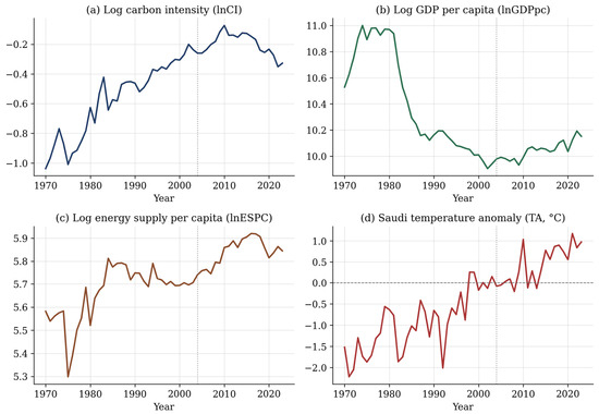
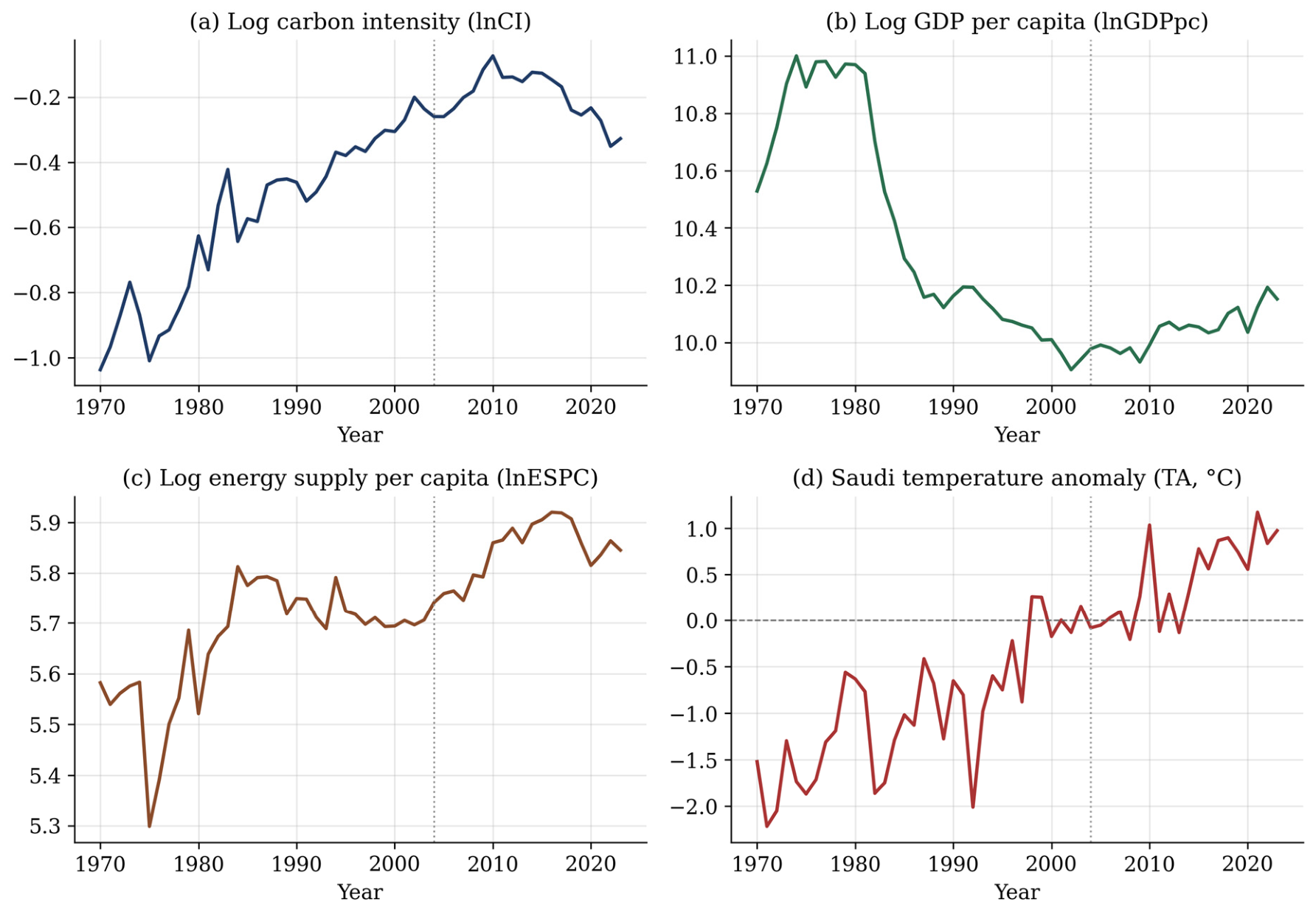
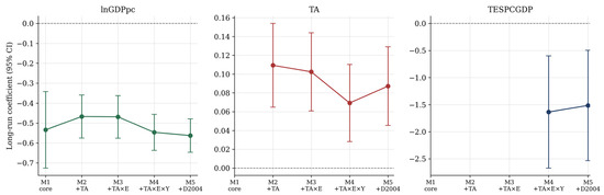
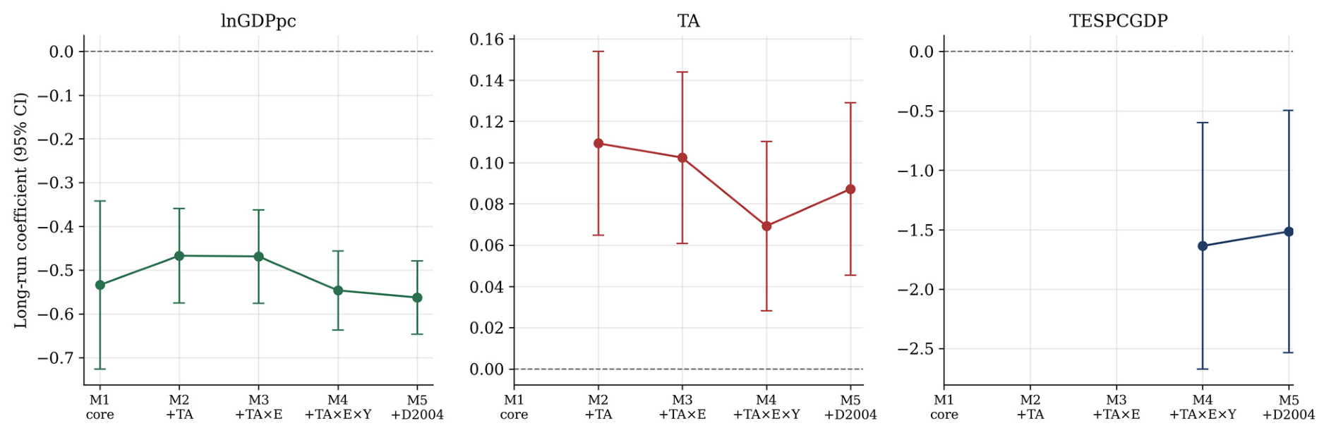
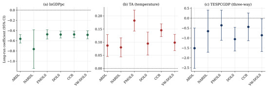
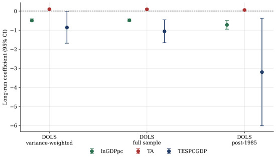
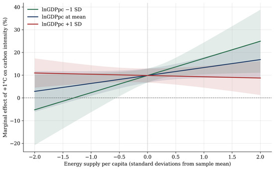
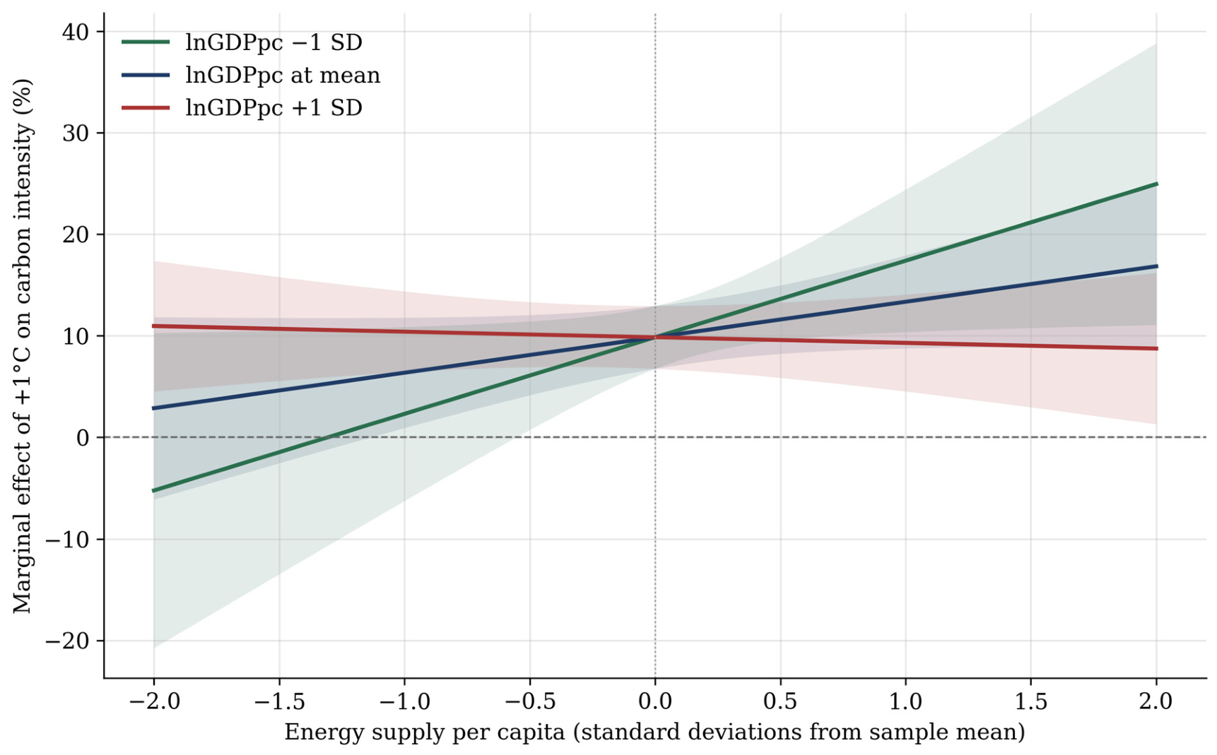
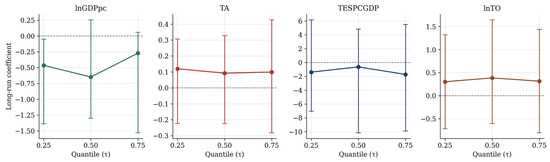
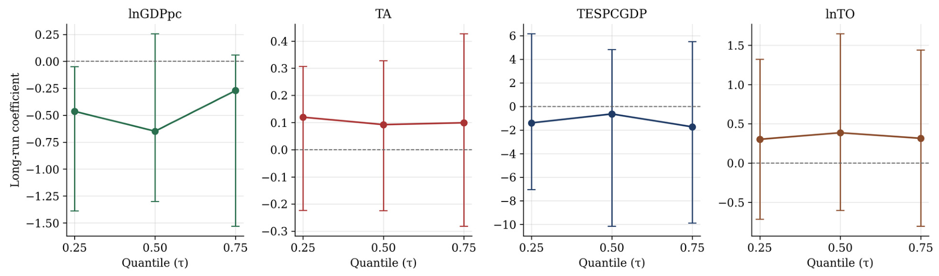
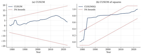
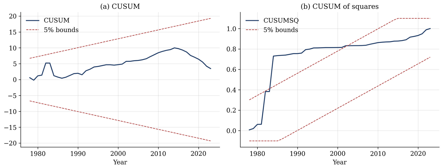

Disclaimer/Publisher’s Note: The statements, opinions and data contained in all publications are solely those of the individual author(s) and contributor(s) and not of MDPI and/or the editor(s). MDPI and/or the editor(s) disclaim responsibility for any injury to people or property resulting from any ideas, methods, instructions or products referred to in the content. |
© 2026 by the authors. Licensee MDPI, Basel, Switzerland. This article is an open access article distributed under the terms and conditions of the Creative Commons Attribution (CC BY) license.