


Abstract
Can China feed itself by 2100? This study begins with a critical reexamination of the bayesTFR recovery assumption embedded in UN WPP 2024 and reconstructs population scenarios using an “empirical-base ± empirical-offset” methodology anchored at China’s 2023 official TFR of 1.01. For food security analysis, we narrow the population to three scenarios (low, medium, and policy target), and we set three scenarios each for the demand side and the supply side, producing an integrated 27-scenario analysis. The demand side comprises three trajectories: East Asian saturation type (650 kg/person/year), EU type (780 kg/person/year), and EU + type (850 kg/person/year). The supply side comprises three trajectories: optimistic (cropland area maintains the red line, with yield reaching the technological ceiling), medium (climate change reduces yield by , and cropland area breaches the red line by ), and pessimistic (climate change reduces yield by , and cropland area breaches the red line by ). Based on NBS empirical data, projection results show that all 27 scenarios achieve surplus by 2100 (even the worst case retains 0.265 Gt surplus), confirming the robustness of long-term food security. However, during the medium term (2030–2050), the worst case scenario retains 26% import dependency. Even under the U.S.-type full emulation scenario (1100 kg/person/year) examined as a supplementary stress test, all nine sub-scenarios maintain surplus. The challenge for China’s food security lies not in long-term absolute shortage but in medium-term import dependency management and policy transition to the surplus era. By integrating demographic projection, agricultural-economic demand modeling, and a layered food-system accounting framework, this study offers a transferable cross-disciplinary methodology for long-term food security assessment under demographic transition, relevant beyond China to other aging, post-peak societies.
Keywords:
food security; population decline; demographic transition; integrated scenario analysis; food supply–demand modeling; interdisciplinary methodology; food surplus; China JEL Classification:
Q11; Q18; J11
1. Introduction
Who will feed China? This question has been debated since Brown’s 1995 monograph. In contrast, this paper offers an inverted perspective: by 2100, China itself, having shrunk to approximately 460 million people, may become a substantial food-surplus nation.
China’s current food-security position is characterized by a long-standing policy commitment to “basic self-sufficiency of grain and absolute security of staple food” (95% self-sufficiency benchmark for grain overall, with rice and wheat fully self-sufficient) [1,2], sustained through the 2024 harvest of 706.5 Mt total grain output (+1.6% YoY), including 652.3 Mt of cereals (+1.7%) [3], despite national drought losses of CNY 8.4 billion. The country nonetheless depends heavily on imported soybeans, accounting for approximately 60% of global soybean trade, primarily sourced from Brazil [4,5]. China’s grain storage capacity exceeded 700 Mt in 2024 (National Food and Strategic Reserves Administration), the world’s largest, providing flexibility well beyond the FAO stock-to-use benchmark of 17–18% (about two months of consumption) discussed in the international food-reserve literature [6], and policy is reaffirmed through the 2014 “Self-Reliance with Domestic Foundation” directive [7] and the 2024 Law on Ensuring Food Security [8]. Against this backdrop of present-day adequacy but underlying soybean exposure and demographic uncertainty, the long-term question of whether China can feed itself by 2100 acquires renewed significance.
The China-specific framing rests on three considerations. First, systemic importance: China accounts for approximately 24% of global cereals-plus-soybeans consumption and approximately 24% of global cereals-plus-soybeans imports (2023/24 marketing year, USDA PSD) [4,5,9], so changes in its demand trajectory produce ripple effects on world markets that are qualitatively distinct from those of smaller importers [10,11]. Second, the limits of the “purchase from international markets” alternative: episodes such as the 2008 food crisis [6,11,12,13] and the 2022 Ukraine war [14,15,16] demonstrate that buy-from-abroad strategies fail under compound geopolitical stress, motivating China’s strategic treatment of self-sufficiency as an independent policy variable. Third, global food-balance implications: if China transitions from net importer to surplus contributor, the pressure released on world markets is comparable in magnitude to sub-Saharan Africa’s entire cereal net import gap [4].
In this paper, we distinguish three related but distinct concepts. Food security follows the FAO four-pillar definition (availability, access, utilization, and stability). Self-sufficiency refers to the quantitative ratio , where is domestic supply and is total demand. Surplus is the flow magnitude when self-sufficiency is achieved. The 27-scenario analysis below evaluates self-sufficiency and surplus as quantitative measures, while food security in the broader FAO sense is discussed in the policy implications (Section 4.2).
China reached its population peak of approximately 1.412 billion in 2021 and has entered a historic demographic transition. The official total fertility rate (TFR) for 2023 was 1.01 [17], and the 2025 birth count of 7.92 million marked a historic low [18]. This rapid fertility decline is consistent with trends observed across East Asia.
The 2024 revision of the United Nations World Population Prospects (UN WPP 2024) [19] projects China’s 2100 population to be 633 million under the medium variant, but this projection depends on the assumption that TFR will recover from the current 1.0 to 1.35 by 2100. However, East Asian empirical data do not support TFR recovery, and the “low fertility trap” hypothesis [20], in which prolonged low TFR forms a positive feedback loop through small-family norm consolidation, decline in reproductive-age women, and rising childcare costs, is materializing.
Most existing population projection studies have adopted UN WPP medium estimates as their baseline. However, the 2023 official TFR of 1.01 diverges from the recovery assumption embedded in UN WPP 2024 medium. Cohort-component estimates [21] and TFR-fixed sensitivity analyses [22] project populations at or below the UN WPP medium, while the IHME GBD framework [23] (CCF50-based) yields a higher value (732 million). All three diverge from the UN WPP medium, indicating significant uncertainty in its recovery assumption.
Population projection forms the foundation for long-term planning in agricultural policy, food security, and rural economy. The choice of population scenario directly impacts evaluations of food demand, self-sufficiency rate, and import dependency. China is the world’s largest food consumer and grain importer, and changes in its demographic dynamics have ripple effects on international grain market stability [24]. For this reason, quantitatively projecting food demand in population-declining China and clarifying the conditions for long-term food security is a priority issue in agricultural policy.
The academic contributions are fourfold: (i) we reexamine the nature of the TFR recovery assumption in the bayesTFR model of UN WPP 2024 and quantify its deviation from 2025 empirical values; (ii) we propose an “empirical-base ± empirical-offset” methodology that anchors at the 2023 official TFR of 1.01 and derives the offset width from East Asian empirical data; (iii) we confirm the validity of the 6-scenario framework through cross-validation using independent estimation methods (cohort-component, TFR-fixed model); and (iv) building on the six population scenarios constructed, we introduce a per-capita total grain demand and a China domestic production projection both anchored to NBS empirical data for base years (2000, 2025), and evaluate total grain demand, supply–demand gap, import dependency, and self-sufficiency equilibrium population from 2000 to 2100 for each scenario. Methodologically, the study sits at the intersection of demography, agricultural economics, and food-system analysis: it couples a cohort-based population reconstruction with a food-balance-sheet demand model and a yield × cropland supply model within a single layered accounting framework. This cross-disciplinary integration is intended to be transferable to other countries undergoing demographic transition, beyond the Chinese case studied here.
2. Materials and Methods
2.1. Population Projection Framework
The fertility projection in UN WPP 2024 is based on a Bayesian hierarchical model (bayesTFR) [25]. This model classifies TFR transitions into three phases, with China and other East Asian countries categorized in Phase III (post-transition). Phase III TFR projections are based on the AR model:
where is the TFR of country c at time t, is the country-specific long-term equilibrium level, is the autoregressive coefficient, and is the error term. tends to be set below the replacement level but above 1.0, and when the current TFR is below , the model mechanically projects TFR recovery. This assumption has several caveats: (i) there is no precedent of countries with TFR below 1.0 (Korea, Spain, and Italy) subsequently sustaining recovery to 1.3 or higher; (ii) East Asia-specific factors (declining marriage rates, late marriage, rising housing and education costs, and gender norm changes) are not incorporated into the AR model; and (iii) although China introduced the two-child policy in 2016 and the three-child policy in 2021, births decreased by 56% from 17.86 million in 2016 to 7.92 million in 2025, indicating limited policy effectiveness. UN WPP 2024 was also revised downward by approximately 17% from UN WPP 2022 [26] across all variants.
The scenario design of this study adopts the principle of “empirical-base ± empirical-offset” in contrast to UN WPP 2024’s “theoretical-equilibrium ± mechanical-offset”. The base point is China’s 2023 official TFR of 1.01 [17], with . This value is the most recent official figure published by the National Bureau of Statistics, consistent with SWUFE’s [22] TFR = 1.05→460 million projection. The offset width is derived from the East Asian empirical range (Table 1). The lower bound () is empirically validated by Korea (TFR 0.72 in 2023, 0.75 in 2024 after a 9-year rebound), and the upper bound () corresponds to the TFR = 1.15–1.20 level achieved by Japan after 30 years of pro-natalist policy. Based on this, we set four core scenarios and two reference scenarios (Table 2).
Table 1.
Latest TFR of East Asian countries and regions.
Table 2.
Scenario definitions: 4 core + 2 reference (design premises only; 2100 population projections shown in Section 3.1).
For 2000–2023, TFR uses common empirical values across all scenarios, diverging by scenario from 2023 onward. The design ensures smooth transitions to long-term levels across the 2030–2040s (Figure 1). Keypoint values are set every 10 years, and annual data are generated by linear interpolation.
Figure 1.
Scenario -based TFR trajectory (2000–2100). The 2023 official TFR = 1.01 serves as the divergence point, with core scenarios (solid lines) and reference scenarios (dashed lines).
To quantify scenario-internal uncertainty, we additionally model each scenario’s TFR as a Gaussian random variable centered at the scenario mean with standard deviation . The value is the empirical standard deviation across six East Asian economies (Korea 0.75, Taiwan 0.89, Japan 1.15, China 1.01, Hong Kong 0.84, and Singapore 0.97; mean 0.935, population SD 0.128), consistent with the empirical-offset width used in scenario design (, corresponding to the standard two-sided 95% coverage interval). Monte Carlo simulation with draws per scenario yields the 95% confidence intervals for the 2100 population reported in Section 3.1. The probabilistic envelope encompasses the deterministic scenario centers and remains well below the self-sufficiency equilibrium population threshold under all supply scenarios, providing a quantified robustness check on the deterministic projections.
The S5 policy-target population of 700 million by 2100 is set as a “peak-halving” reference, approximately half of China’s 2021 demographic peak of 1.412 billion (NBS [17]). This symbolic threshold carries three complementary interpretations: (i) demographically, the post-transition completion benchmark at which the population reaches half of its historical maximum; (ii) historically, the level last sustained around 1965 when China’s population was approximately 720 million, demonstrating viability under far lower agricultural productivity than today; and (iii) narratively, the symbolic anchor for the inversion of Brown’s [27] question, framing China’s transition from “the 14-billion-people food problem” to “the halved-China food surplus”. The central conclusion of this study (surplus emergence across all 27 scenarios) does not depend on the specific S5 value.
Using this population target as input, we compute the fixed TFR required to reach 700 million by 2100 via cohort-component dynamics. Linear regression across the deterministic scenarios (S1: TFR = 0.75 → 320 M; S2: TFR = 1.00 → 460 M; S3: TFR = 1.25 → 660 M) yields the near-perfect relation (M). Setting M gives TFR , which we adopt as the fixed simulation value for S5 (listed as ≈1.31 in Table 2; the corresponding 10-year keypoints are presented in Section 3.1). We emphasize that 700 M at 2100 does not represent a demographic steady state: under TFR = 1.31, S5 shows 820 M at 2090 still declining at ∼12 M/yr, so 700 M is an end-period value during continued sub-replacement decline; true demographic stationarity would require TFR near the replacement level (≈2.05). The 700 M target is also only 46–64% of the self-sufficiency equilibrium population (the population at which demand equals domestic supply: approximately 1.54 billion under optimistic supply S-O, 1.32 billion under medium S-M, and 1.10 billion under pessimistic S-P; see Section 3.5), so S5 provides a substantial food-surplus margin under all supply scenarios. The required TFR = 1.31 is, however, ambitious: it exceeds the 2024 levels of Japan (1.15, MHLW), Finland (1.25, an all-time low recorded by Statistics Finland), Spain (1.10, INE), and Italy (1.18, ISTAT), all of which hit historic lows in 2024. Sustained East Asian pro-natalist policy efforts in Korea, Japan, and Singapore have not historically delivered TFR increases beyond to , placing 1.31 at the upper edge of the empirical policy-effect range from a 1.01 base. S5 is therefore best characterized as a reference scenario for policy discussion, anchored on peak halving, rather than as a standalone demographic projection.
2.2. Apparent Consumption via the Food Balance Sheet Approach
This study adopts the apparent consumption approach, which is the food balance sheet method officially used by FAO and NBS. It directly derives the per-capita total grain demand from empirical data on domestic production, trade, and population:
where is domestic grain production (NBS Grain broad: grains + soybeans + tubers), and are imports and exports of grains (cereals) and soybeans, and is total population. Equation (2) defines demand (=production + imports − exports), not actual consumption; stock variation is by definition not part of . Since this study projects demand rather than actual consumption, there is no need to subtract from the equation. The meaning of is clarified by the algebraic identity , so the supply–demand gap equals net imports.
Data sources are cross-validated across three systems: (i) domestic production from NBS official annual bulletins [18]; (ii) trade data from USDA PSD (Production, Supply, and Distribution) [4] and FAOSTAT Trade [9]; and (iii) population from World Bank/NBS. Table 3 shows the empirical trajectory from 2000 to 2024.
Table 3.
China’s apparent per-capita grain consumption (2000–2024 empirical, NBS Grain broad).
The observed trajectory shows that increased from 371 kg/person/year in 2000 to 590 kg/person/year in 2024, a rise (annual average /yr). This reflects the rapid expansion of feed grain demand driven by rising income, urbanization, and meat consumption.
2.3. Food Demand Model
China’s total grain demand (Gt/yr) is expressed as a simple multiplicative form of population and per-capita total grain demand (kg/person/year):
where is the apparent per-capita consumption defined in the previous section (Equation (2)), which does not require separate multiplication by age-stratified basic consumption or feed conversion ratio. The empirical trajectory (2000–2024) is fixed to the annual values in Table 3 (371→590 kg/person/year, /yr). The future trajectory (2025–2100) is extrapolated based on the cumulative income adjustment factor and urbanization effect cumulative adjustment factor , as :
where is the annual growth rate of per-capita real GDP (income) at time s (%/yr), is the annual change in urbanization rate at time s (percentage points/yr), is the income elasticity, is the urbanization elasticity, and is the base year. ∏ denotes the cumulative multiplication of each year’s effect from to t. We adopt and .
The selection rationale and validation of parameters are as follows. The income elasticity falls within the central range of: Yu & Abler [28] (grain elasticities 0.08–0.39 from Table 3; 26-province rural panel for 1994–2003); Chen et al.’s [29] meta-analysis (reported cereal elasticities 0.42–0.49 with documented decay toward projected mid-century values ∼0.15–0.30); and is consistent with the long-term demand-projection assumptions of FAO/Alexandratos & Bruinsma [30]; it also lies within the standard deviation range of Zhou et al.’s [31] meta-analysis mean ( SD 0.34). The urbanization elasticity captures the diminishing marginal effect as China approaches urbanization saturation, aligning with OECD-FAO Agricultural Outlook projections (0.05–0.15, China 2020+) and Zhou et al.’s [31] urban subsample evidence of demand-side maturation. These parameters fit the empirical (371→590 kg/person/year, 2000–2024) with annual mean error , RMSE , and exact match at the 2024 validation point (predicted 590 = empirical 590).
The long-term paths of and are set to reflect gradual deceleration accompanying the maturation of China’s economy. Specific rationales: (i) = 5% in 2025 is consistent with NBS empirical data (2020–2024 average); (ii) = 4% in 2030 follows World Bank “China 2030” and long-term extrapolation of the 14th Five-Year Plan; (iii) = 1.5–2% from 2050 onward follows the regression-to-the-mean prediction of Pritchett & Summers [32] for long-run growth, where mature economies like Korea and Japan illustrate the typical post-convergence trajectory; (iv) follows the UN World Urbanization Prospects trajectory from 67% in 2024 to 73–75% in 2050 and saturation at 75–80% from 2075 onward. The annual paths are designed to decelerate progressively over 2025–2100, and the corresponding trajectory is shown in Section 3.3.
Under alone, would continue to grow at 0.35–0.47%/yr in 2050–2100, reaching approximately 850 kg/person/year cumulatively. However, following Bennett’s Law and empirical observations from high-income countries (US/EU 1000–1100, OECD average ≈800 kg/person/year), grain-equivalent consumption saturates when income exceeds a certain level due to qualitative diversification of diet. We introduce this saturation effect as an upper-bound function:
where kg/person/year (asymptotic upper bound near OECD average), (asymptotic speed), and kg/person/year. For , dominates; for , the second term (saturation path) dominates. The specific trajectory values of the three demand scenarios (D-L/D-M/D-H) and three supply scenarios (S-O/S-M/S-P), together with the basis for anchoring each to the 2024 observed value, international comparison, and the literature projections, are set out collectively in Section 3.2, following the extraction of population scenarios (Section 3.1).
The 2100 endpoints of the three demand trajectories (D-L = 650, D-M = 780, D-H = 850 kg/person/year) are anchored as follows. D-L = 650 corresponds to the upper envelope of recent East Asian saturated economies, bracketed by Japan (470) and Korea (580) with allowance for moderate further intensification, and is consistent with the empirical observation that no East Asian economy has sustained above 700 kg/person/year. D-M = 780 corresponds to the midpoint of the income-and-urbanization elasticity projection under (760–800) and matches the asymptotic ceiling in Equation (6). D-H = 850 sits at the midpoint between the EU average ( = 700, meat 80 kg/person/year), and the U.S. level ( = 1100, meat 120), with meat at 95 kg/person/year as a high-saturation upper bound. Demand drivers beyond income and urbanization, including dietary policy (Healthy China 2030 meat-suppression targets), environmental constraints (carbon-neutrality 2060 livestock limits), alternative proteins (the rapid expansion of plant-based and cultivated meat markets), and consumer preferences (Z-generation flexitarian shift), further motivate the saturation interpretation of D-L and the calibration of D-M.
2.4. Demand Structural Decomposition
The apparent consumption in the previous section aggregates all uses (food, feed, industrial, and others). To clarify the drivers of demand growth, this section decomposes into four sectors and models the largest sector, feed grain, as an independent variable.
Per-capita total grain demand is decomposed into four sectors: direct consumption (food), feed use, industrial use, and other (seed, loss, etc.):
Among these, feed grain is expressed as the product of per-capita meat consumption (kg/person/year) and the feed coefficient (kg grain per kg meat):
where is total feed grain demand (Gt/yr). Thus feed grain demand is the product of three factors: population, diet (meat consumption), and livestock technology (the feed coefficient).
The feed coefficient is the effective value obtained by multiplying the weighted average of livestock-specific FCR (Table 4, currently ≈3.74) by the grain share of feed (excluding forage and food residues). From 2000–2024 empirical data, and . This rise reflects the intensification of Chinese livestock (transition from forage dependence to compound feed). For the future, a shift toward poultry (FCR 2.0) and scale-driven FCR improvement offset continued intensification, and is assumed to converge to . The convergence to FCR = 3.0 is consistent with the feed-efficiency improvements documented in European livestock LCA research [33] and FAO long-term projections of similar trends [30,34].
Table 4.
Livestock-specific FCR and weighted average for China (basis for the upper bound of feed coefficient ; composition from NBS [17]).
Per-capita meat consumption expanded from 53 kg/person/year in 2000 to 75 kg/person/year in 2024 (mainly pork and poultry). The future trajectory follows the three demand scenarios (D-L low, D-M medium, and D-H high; 650/780/850 kg/person/year, defined in Section 3.2), with meat consumption reaching 60 (D-L), 90 (D-M), and 95 (D-H) kg/person/year in 2100. The D-H value of 95 kg/person/year is a high-saturation level, lying between the EU average (80) and the U.S. (120).
By Equation (8), feed grain is estimated at kg/person/year in 2024 (42% of ) and kg/person/year in 2100 under D-M. The remaining food, industrial, and seed/loss sectors evolve as follows: food declines due to aging and urbanization (from 177 in 2024 to about 140 kg/person/year in 2100), industrial use expands moderately with bioethanol and starch sugar demand, and the seed/loss component contracts as post-harvest losses are reduced. Table 5 presents the four-sector decomposition for empirical years and the 2100 food structure scenarios.
Table 5.
Four-sector structural decomposition of (kg/person/year) and 2100 food structure scenarios.
Feed-grain modeling identifies feed conversion (meat consumption × feed coefficient), rather than direct food consumption, as the dominant driver of demand growth. As of 2024, feed use accounts for 42% of , and of the 2000–2024 increase in (371→590, kg/person/year), the feed contribution is kg/person/year (57%).
2.5. Chinese Domestic Production Projection Model
The domestic production model in this study is constructed using NBS (National Bureau of Statistics) empirical values and the apparent consumption defined in Section 2.2 (Equation (2)). As a basis for projection, two reference points (base year 2000 and most recent empirical year 2025) are anchored to empirical values, with the intervening period and future connected by continuous trajectories directly derived from empirical data.
Base year 2000 values are as follows: Gt (NBS Grain broad, 2000 official); kg/person/year (Table 3; Gt; billion); Gt. For the most recent empirical year 2025, Gt (NBS 2025 official); kg/person/year (extrapolated at /yr from 590 in 2024); Gt, self-sufficiency rate , consistent with 2024 net imports of 0.124 Gt. A summary of base values is shown in Table 6.
Table 6.
Reference values for projection based on NBS empirical data.
is given as the product of yield (kg/ha) and cropland area (ha):
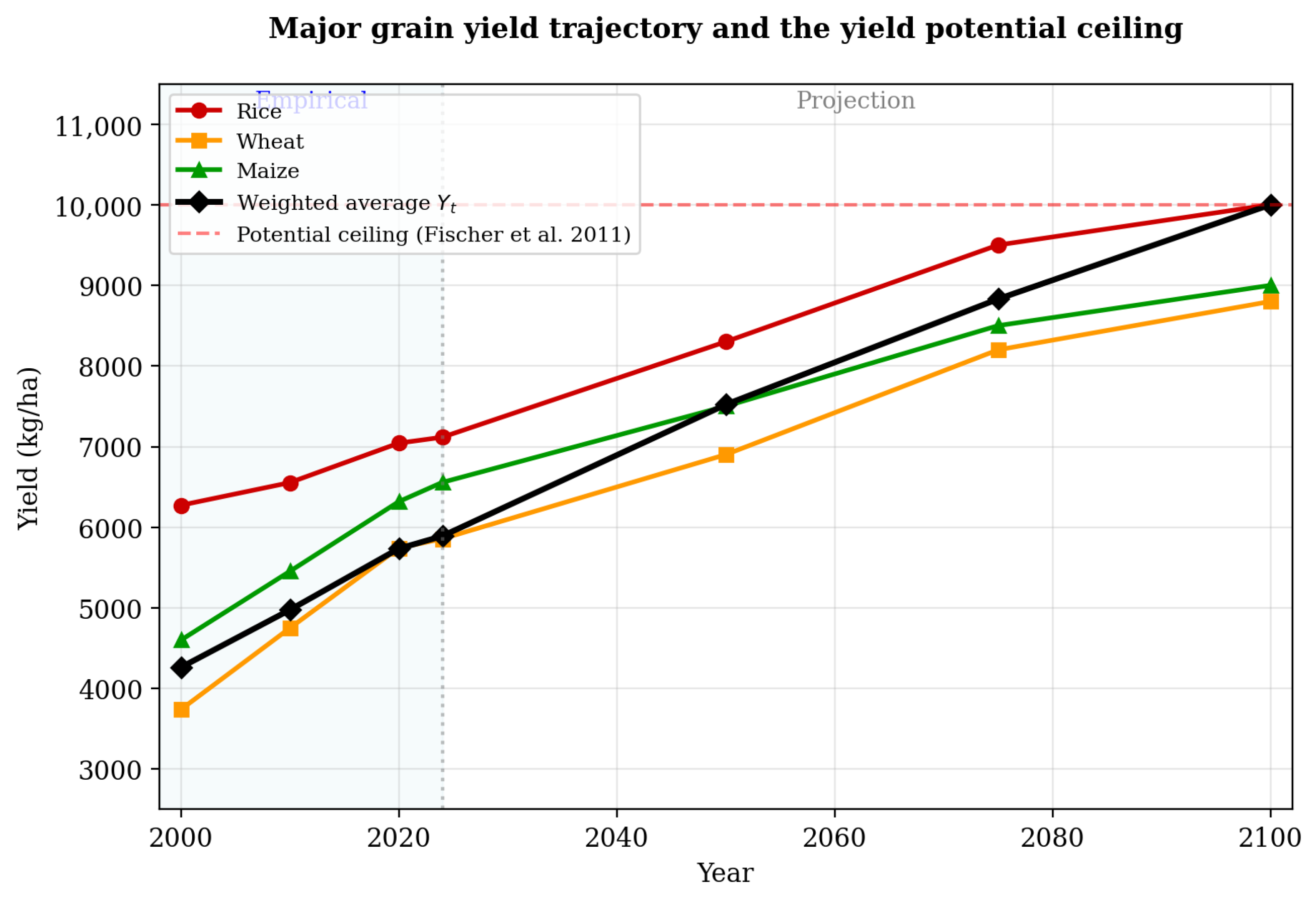
Table 7 shows empirical and future estimates of yield and cropland area for major grains. China’s major grain yields grew at /yr from 2000 to 2024, with the national weighted average reaching 4261→5890 kg/ha. Cropland area was 130 Mha in 2000, evaluated at 128 Mha in the Third National Land Survey (2020), and it reached 129.3 Mha (1.94 billion mu) as of the end of 2024 after consecutive annual recoveries, with a 7.7% margin to the red line of 120 Mha.
Table 7.
Empirical and projected major grain yields (kg/ha, weighted average) and cropland area (Mha).
Figure 2.
Major grain yield trajectory and the yield potential ceiling (10,000 kg/ha, Fischer et al. 2011 [36]).
The long-term trajectory of domestic grain production is given as a simple compound of period-specific growth rates with gradual deceleration, anchored to the two empirical reference points:
where the period-specific growth rate decelerates progressively as shown in Table 8.
Table 8.
Period-specific growth rates and piecewise trajectory of domestic production .
In units of Gt/yr, the Gt ceiling is determined by the yield potential of approximately 10,000 kg/ha ([36], Ch. 10) and the cropland red line of 120 Mha (=1.8 billion mu, theoretical maximum) [35]. Domestic grain production is independent of population scenarios; it is determined by yield (kg/ha) × cropland area (ha), and population scenarios act only through the demand side.
From the total demand formulated in Section 2.3 and the domestic production of this section, the supply–demand gap and import dependency are defined as follows:
where is the supply–demand gap (Gt, positive = shortage, negative = surplus), is the import dependency (%, share of shortage relative to total demand, 0 when surplus).
The yield ceiling of 10,000 kg/ha adopted in the S-O scenario reflects the technological potential identified by Fischer et al. [36]; this assumption is consistent with global yield-gap analyses [37,38,39], but its realization depends on three institutional factors. First, economic feasibility: achievement of the ceiling assumes sustained agricultural R&D investment at the upper tier of high-income agricultural economies (such as Korea, Japan, and Israel). According to the OECD’s Innovation, Agricultural Productivity and Sustainability in China assessment, China’s agricultural R&D intensity, while growing rapidly in absolute terms (China is the world’s largest investor in public agricultural R&D in money terms), still lagging behind those of the United States and other higher-income Asian countries when measured as a share of agricultural GDP. Second, environmental costs: realizing the yield ceiling assumes substantial improvements in nitrogen-use efficiency (target 60% versus approximately 30% at present) and irrigation efficiency (target 70% versus approximately 58% at present), addressing the eutrophication and water-table-decline concerns identified by Wang et al. [40]. Third, long-term sustainability: the 10,000 kg/ha figure represents technological potential under best-management practices, whereas the S-M scenario (9000 kg/ha) represents a realistic operational level in the absence of full institutional transformation. Thus S-O is positioned as the upper-bound case under ideal conditions, S-M as the operational level under realistic conditions, and S-P as the lower-bound case under composite degradation.
2.6. Climate, Water, and Land Constraints and the Supply Scenarios
This model adopts the cropland red line (minimum 120 Mha) and yield potential as production constraints, and incorporates climate, water resources, and land constraint impacts into the three supply scenarios (S-O optimistic, S-M medium, and S-P pessimistic, defined in Section 3.2) (Figure 3). Specifically, S-M (medium) assumes climate impact and red-line breach, while S-P (pessimistic) assumes climate impact and red-line breach.
Figure 3.
Components of the three supply scenarios. (a) Yield trajectory: S-O optimistic reaches the yield potential of 10,000 kg/ha, S-M medium reaches 9000 under climate impact , and S-P pessimistic reaches 8000 kg/ha under climate impact . (b) Cropland area trajectory: S-O optimistic maintains the cropland red line of 120 Mha, S-M medium breaches it by (114 Mha), and S-P pessimistic by (108 Mha). The supply scenarios S-O/S-M/S-P are defined in Section 3.2.
Regarding the impact of climate change on Chinese agriculture [41,42,43], Chou et al. [44] use an economy–climate (C-D-C) model to project grain yield changes for China, Japan, and Korea, showing that from 2021 to 2050 climate change exerts positive impacts on rice and wheat yields in China (with regional and SSP-dependent variation), while maize is negatively affected; risks vary widely across regions and crops. Tao et al. [45] used 1981–2009 empirical data to analyze wheat impacts across China’s major climate zones, showing that warming effects vary by region (increases of to in northern zones, and decreases of to in southern zones). Zhao et al.’s [46] meta-analysis of four independent models shows global average yield decline per 1 °C temperature increase of rice , wheat , maize , and soybean (including Chinese data). These China-specific findings are consistent with global cross-sectional evidence on climate–yield relationships [47,48,49] and with documented increases in adverse weather frequency under warming [50]. This study’s S-P scenario assumes a climate impact, which lies within the range implied by linear extrapolation of the above per-°C estimates to 4 °C warming (wheat: from both Asseng et al. [49] and Zhao et al. [46]; maize: from Zhao et al. [46]). This assumption is empirically bounded and represents a conservatively pessimistic case. Note that climate impacts show significant regional and crop-specific differences, with North China Plain maize and wheat being most affected.
Regarding water resource constraints [51,52], Wang et al.’s [40] evaluation of China’s water resources and food security indicates that groundwater levels in the North China Plain declined by 1.0–1.5 m/yr on average during the period leading up to 2017, with agricultural groundwater depletion identified as one of China’s most serious resource problems threatening food security. Liu et al.’s [53] global water resource assessment also classifies the North China Plain as one of the most water-stressed agricultural regions worldwide. More recent evidence indicates that groundwater levels have begun to recover at approximately m/yr since 2020, driven by South-to-North Water Transfer Project deliveries and stricter pumping regulations, with 2024 levels surpassing those of 2005. This partial recovery reduces the near-term severity of the constraint but does not eliminate the aforementioned structural vulnerability; long-term sustainability under climate change remains uncertain. Limitations of the South-to-North Water Transfer Project, combined with precipitation pattern changes from climate change, suggest agricultural water may decrease by 15% or more by 2050. This directly impacts North China irrigated agriculture (60% of China’s wheat production and 40% of maize production). The S-P scenario in this study collectively incorporates these climate impacts and water resource constraints as climate reduction.
Cropland quality degradation includes soil degradation from excessive chemical fertilizer input, heavy metal contamination, and salinization. These factors hinder achievement of yield potential, potentially causing downward deviation from Fischer et al.’s [36] theoretical maximum of 10,000 kg/ha. The S-M and S-P scenarios collectively represent these composite degradation factors as yield reduction.
The three supply scenarios use mean yield reduction as a proxy for diverse climate-related stresses. As a further stress test, we define a compound-stress scenario S-XP in which climate impact is combined with an additional drought-and-event premium (total , yield 7000 kg/ha) and the red-line breach is deepened to (cropland 102 Mha). S-XP represents a compound climate-and-land stress that conservatively exceeds the IPCC AR6 SSP5-8.5 envelope and lies outside the principal 27-scenario axes; quantitative results for S-XP are reported at the end of Section 3.3.
3. Results
3.1. Population Projection Results and Extraction of Three Scenarios for Food Security Analysis
Table 9 shows the population trajectory for six scenarios (10-year keypoints and 2020-baseline decline rate). All scenarios peak around 2021 at approximately 1.412 billion and then decline (Figure 4). The empirical baseline S2 projects 460 million by 2100, a 68% population decline from 2020. Even the high S3 scenario (660 million) implies a 54% decline, and even the substantial recovery scenario S6 falls to 954 million (a 33% decline).
Table 9.
Scenario-based population trajectory (billion, every 10 years).
Figure 4.
Scenario-basedpopulation trajectory (2000–2100). Core scenarios (S1–S3, solid lines) and reference scenarios (S4–S6, dashed lines). All scenarios peak around 2021, then decline.
Incorporating TFR uncertainty via the probabilistic framework introduced in Section 2.1 (, draws), the 2100 population 95% confidence intervals are as follows: S1 million (median 322), S2 million (median 459), S3 million (median 660), and S5 million (median 699). The upper bounds across all scenarios remain well below the self-sufficiency equilibrium population thresholds reported in Section 3.5 (1.10–1.54 billion depending on supply scenario), confirming that surplus emergence is robust to scenario-internal TFR uncertainty. In particular, even the 97.5th percentile upper bound of S5 (875 million) sits below the S-P (pessimistic supply) equilibrium of 1.10 billion, so the qualitative conclusion of long-term surplus is preserved across the entire TFR uncertainty envelope.
For food supply–demand analysis, we narrow the six scenarios to three to consolidate the discussion. S4 and S6 are close to S3 and S5, respectively, and they are merged, and S3 has limited difference from medium S2, so S5 serves both as the policy target and upper bound. We finally adopt low P1 (=S1, Korean type, 320 million), medium P2 (=S2, status quo, 460 million, empirical baseline), and policy target P3 (=S5, 700 million). These three scenarios cover the East Asian empirical TFR range of 0.75–1.31 and provide the population width necessary for food security analysis (320–700 million).
Population decline in S2 (status quo) is not constant but accelerating. From 2020 to 2050 (30 years), the decrease is 232 million (average 7.73 million/yr), while from 2050 to 2100 (50 years), the decrease is 734 million (average 14.68 million/yr), with the latter half’s decline rate approximately doubling. This is because the population of reproductive-age women (20–39) decreases exponentially, reflecting the feedback structure of the “low fertility trap”. Inter-scenario differences are relatively small in 2030 (1.373–1.413 billion, width 40 million), indicating limited room for policy intervention. However, by 2100, the difference between S1 (320 million) and S6 (954 million) expands to 634 million, making clear that TFR assumption differences have decisive long-term impact.
Population aging also progresses rapidly. According to Li & Zhou’s [21] CPPS projection, when TFR = 1.0, the elderly ratio (65+) reaches 53.91% by 2100. Aging affects labor supply, social security, and consumption patterns, but since this study’s food demand model uses apparent consumption , age structure changes do not directly affect demand projection.
Table 10 shows the year-of-publication ordered comparison of major population projections. The trend of downward revision with later publication year is clear.
Table 10.
Year-ordered comparison of China’s 2100 population projections.
This study’s results show consistency with independent projections (Table 11, Figure 5). S2 (460 million) exactly matches Southwestern University of Finance and Economics (SWUFE) [22] TFR = 1.05 fixed projection (460 million), mutually validating through convergence of independent methods. In Li & Zhou’s [21] CPPS projection, the TFR = 1.2 scenario (634 million) falls between S3 (660 million, ) and S4 (633 million, ). The common finding of both studies is that 2100 population falls in the 500–700 million range under TFR = 1.0–1.2.
Table 11.
China 2100 population projection: comparison with the major literature.
Figure 5.
China 2100 population projection: comparison with major literature. Sources shown in the image: UN WPP 2022 [26], IHME [23], UN WPP 2024 [19], Li-Zhou CPPS [21], SASS [54], and SWUFE [22]. Red is this study, orange is SWUFE, blue is UN WPP 2024. This study S2 (460 million) and SWUFE (460 million) independently converge to the same result.
3.2. Design and Demand/Supply Trajectories of 27-Scenario Integrated Analysis
To evaluate the robustness of food security, we conduct an integrated 27-scenario analysis with 3 population scenarios × 3 demand scenarios × 3 supply scenarios.
On the demand side, we set three future trajectories of per-capita total grain demand based on international comparison. D-L (low saturation, 650 kg/person/year, East Asian saturation type) corresponds to progress in health orientation and alternative protein adoption. D-M (medium, 780 kg/person/year, EU type) is the baseline, consistent with the OECD-FAO Outlook. D-H (high saturation, 850 kg/person/year, EU + type) is a high-saturation case based on international comparison, above the EU average ( = 700, meat 80 kg/person/year) but below the U.S. (1100, meat 120), with meat at 95 kg/person/year (between the EU and the U.S.). The U.S.-type full emulation (D-X: 1100 kg/person/year) is culturally and health-policy-wise difficult and is examined separately as an additional stress test in Section 3.5.
All three trajectories share the 2024 observed value of 590 kg/person/year as a common starting point, and are constructed by anchoring the 2100 endpoints (D-L 650, D-M 780, and D-H 850) to high-income country empirics and international comparison. The medium scenario D-M’s 2050 value of 740 kg/person/year is the reference trajectory consistent with the medium-term projections of DRC (Development Research Center of the State Council, 700), OECD-FAO Agricultural Outlook, and IFPRI IMPACT (600–700), and matches the elasticity-based projection with and . The low D-L (2050 = 680) and high D-H (2050 = 800) are set as scenario assumptions that bracket this literature range from below and above, framing D-M between low- and high-end cases. Intermediate years are interpolations from the 2024 starting point reflecting income-growth deceleration, and the period-by-period growth rates implied by Table 12 are derived results of these anchored trajectories.
Table 12.
Trajectories of three demand/supply scenarios (Gt or kg/person/year).
On the supply side, three scenarios are set by combinations of yield and cropland . S-O (optimistic, kg/ha, Mha, Gt) corresponds to Fischer et al.’s [36] yield potential with the cropland area maintaining the red line. S-M (medium, , Mha, Gt) corresponds to a climate impact of exceeding the upper range of Chou et al. [44] and a red-line breach. S-P (pessimistic, , Mha, Gt) corresponds to a climate impact of conservatively exceeding Chou et al.’s range, combined with a red-line cropland breach (scenario assumption). On the population side, we adopt S1, S2, and S5 (P1 = 320 million, P2 = 460 million, and P3 = 700 million). Keypoint values of these demand/supply trajectories are shown in Table 12.
The interpolation method for the cropland trajectory of each supply scenario is shown in Table 13. Starting from the 2024 empirical value (129.3 Mha), cropland is linearly interpolated to each scenario’s target level by 2050 and assumed to stabilize at the red line or breach level thereafter.
Table 13.
Cropland area trajectory of the three supply scenarios (Mha).
The long-term supply–demand trajectory is shown in Figure 6. Demand under the baseline (P2 × D-M) peaks at around 0.89 Gt in the late 2030s, then contracts to 0.359 Gt by 2100 due to population decline and the saturation effect of . Supply reaches 1.20 Gt by 2100 under red-line maintenance (S-O) and retains 0.86 Gt even under the pessimistic scenario (S-P). Their crossover shifts all scenarios into the surplus region after 2050.
Figure 6.
Long-term supply–demand trajectory of China (2000–2100). Three supply scenarios (blue solid lines) and the three main demand trajectories (red, orange, green). The green area is the surplus region of the baseline (P2 × D-M). Even the worst case P3 × D-H × S-P retains a 0.265 Gt surplus in 2100.
3.3. 27-Scenario 2100 Results: All Achieve Surplus
Figure 7 summarizes the 2100 supply–demand gap for all 27 scenarios. Demand and gap (negative = surplus) are computed, and three panels (P1/P2/P3), each a grid of demand (vertical: D-L/D-M/D-H) against supply (horizontal: S-O/S-M/S-P), show every combination with color (blue = surplus, red = shortage) and the numeric value. Moreover, #1–#27 are numbered in the order population → demand → supply. All 27 scenarios achieve surplus, with the worst case #27 (P3 × D-H × S-P) retaining 0.265 Gt surplus, the best case #1 (P1 × D-L × S-O) 0.992 Gt, and the empirical baseline #13 (P2 × D-M × S-O) 0.841 Gt. This demonstrates the robustness of long-term food security.
Figure 7.
Summary heat map of the 2100 supply–demand gap (Gt) for the 27 scenarios. Three panels correspond to the population scenarios (P1/P2/P3); each grid maps demand (D-L/D-M/D-H) against supply (S-O/S-M/S-P). Negative values (blue) = surplus, positive (red) = shortage. All 27 cells are negative; the worst case #27 (P3 × D-H × S-P) retains a Gt surplus, while the best case #1 (P1 × D-L × S-O) reaches Gt.
As a supplementary stress test, the S-XP scenario defined in Section 2.6 (climate and red-line breach ) represents a compound stress that conservatively exceeds the IPCC AR6 SSP5-8.5 envelope and lies outside the principal 27-scenario axes. Under S-XP, 2100 production falls to yield 7000 kg/ha × cropland 102 Mha Gt. Against the worst-case demand combination P3 × D-H ( Gt), a surplus of Gt remains. The robustness of surplus emergence is therefore confirmed even under this compound climate-and-land stress, although S-XP is reported as a stress-test axis rather than as a primary projection.
3.4. Medium-Term 2030 and 2050 Supply–Demand Gap
The medium term (2030–2050), in which population decline has not yet progressed and demand expansion is still active, presents the highest import dependency risk in our framework. This section describes the medium term from four perspectives: (i) representative cases, (ii) the full 27-scenario outcome at 2050, (iii) uncertainty via the median and quantile range, and (iv) the timing of permanent self-sufficiency.
3.4.1. Representative Cases
Table 14 shows the 2030 and 2050 supply–demand gap and import dependency for the best, baseline, and worst cases. The worst case (P3 × D-H × S-P) reaches 24.3% import dependency in 2030 and 26.4% in 2050, while the baseline (P2 × D-M × S-O) reverts from 12.8% dependency in 2030 to a small surplus by 2050. The best case (P1 × D-L × S-O) holds dependency to 10.5% in 2030 and reaches a 0.163 Gt surplus by 2050.
Table 14.
Supply–demand gap for representative cases in 2030 and 2050.
3.4.2. All 27 Scenarios at 2050
At 2050, 17 of the 27 scenarios (63%) remain in shortage, and the remaining 10 (37%) have already shifted to surplus (Table 15). The largest shortage is #27 (P3 × D-H × S-P) at Gt (26.4% dependency), and the largest surplus is #1 (P1 × D-L × S-O) at Gt. The baseline #13 (P2 × D-M × S-O) is already in a small surplus ( Gt), but shortages remain whenever demand reaches D-M or higher and supply falls to S-M or below. With a majority still in shortage at 2050, this period is when import-dependency management matters most, and the combinations of demand scenario (D-L/D-M/D-H) and supply shock (S-M/S-P) account for most of the medium-term uncertainty.
Table 15.
The 2050 supply–demand gap for the 27 scenarios (Gt, negative = surplus). Parenthetical values give the import dependency when .
3.4.3. Timing of Permanent Self-Sufficiency
Figure 8 maps the year in which each scenario crosses into permanent surplus. The earliest is 2039 (#1, P1 × D-L × S-O) and the latest is 2079 (#27, P3 × D-H × S-P); all 27 scenarios reach permanent self-sufficiency by 2079. The baseline #13 (P2 × D-M × S-O) reaches self-sufficiency in 2047, and more than half of the scenarios transition by the 2050s. The combinations that hold P3 population while combining high demand and pessimistic supply (#25–#27) push the crossover year to 2060–2079.
Figure 8.
Year of permanent self-sufficiency for each of the 27 scenarios. Three panels correspond to the population scenarios (P1/P2/P3); each grid maps demand against supply. Lighter cells indicate earlier crossover (late 2030s) and darker cells indicate later crossover (late 2070s). All combinations reach permanent self-sufficiency by 2079.
3.5. Self-Sufficiency Equilibrium Population and Robustness Verification
The population at which total grain demand equals domestic production is defined as the self-sufficiency equilibrium population . Calculated by supply scenario (D-M = 780 kg/person/year basis),
Even under the worst supply S-P, the self-sufficiency equilibrium population is 1.10 billion, far exceeding P3 = 700 million.
As an additional stress test, we examine U.S.-type full emulation (D-X = 1100 kg/person/year). All nine sub-scenarios maintain surplus, with a worst margin of 0.090 Gt at P3 × D-X × S-P. Since reaching D-X is culturally and health-policy-wise difficult, this does not affect the main conclusion.
3.6. Parameter Sensitivity Analysis
To identify which model parameters most influence the 2100 supply–demand gap G, we perform a deterministic tornado sensitivity analysis (Figure 9). Each of five key parameters is perturbed by a characteristic deviation from its baseline value while all other parameters are held at their baseline, and the resulting change is computed. The characteristic deviation is empirically grounded and comparable across parameters: for demand-side parameters () it corresponds to the empirical standard deviation across the central literature estimates cited in Section 2.3, and for supply-side parameters (yield ceiling and 2100 cropland) it corresponds to the half-spread of the deterministic supply scenarios (S-O/S-M/S-P) defined in Section 2.6. Specifically: income elasticity , (half-spread of the central literature estimates discussed in Section 2.3); urbanization elasticity , (half-spread of the saturation-stage estimates derived from OECD-FAO and Zhou et al.’s [31] urban subsample analysis); long-term income growth , (half-spread of central long-term projections by IMF, World Bank, and OECD); yield ceiling 9500 kg/ha (midpoint of S-O and S-M), (the deterministic-scenario spread, covering S-O 10,000 and S-M 9000); and 2100 cropland 114 Mha (equal to S-M), (half-spread of deterministic S-O 120 and S-P 108).
Figure 9.
Tornado sensitivity of the 2100 supply–demand gap G to characteristic-deviation perturbations of five input parameters (demand-side: empirical literature SD; supply-side: half-spread of the deterministic supply scenarios). Yield ceiling and cropland area dominate; income/urbanization elasticities are damped by the saturation cap.
The tornado analysis ranks the drivers of as follows: (1) yield ceiling ( Gt), (2) cropland area (0.057 Gt), (3) long-term income growth (0.018 Gt), (4) income elasticity (0.005 Gt), and (5) urbanization elasticity (0.002 Gt). Supply-side capacity parameters dominate the sensitivity, with demand-side elasticities entering only after the saturation cap of Equation (6) substantially limits their influence beyond 2050. This pattern indicates that policy levers most consequential for the magnitude of surplus are those that bear on yield realization and red-line maintenance, not on income or urbanization dynamics.
Even the worst characteristic-deviation combination of yield ceiling (8500 kg/ha) and cropland (108 Mha) yields Gt, well above the baseline demand Gt under P2 × D-M, preserving the surplus conclusion.
4. Discussion
4.1. Historical Context: Reexamining the Brown Argument
How can Brown’s prediction be evaluated 30 years later? The question raised by Lester Brown in 1995 in Who Will Feed China? [27] has been a central topic of international food security debate. Brown’s pessimistic prediction (that China would import over 200 Mt of grain by 2030 and disrupt world markets) has been partially realized. China’s grain imports in the 2020s are in the 120–160 Mt/yr range, approaching Brown’s projection. However, Brown did not foresee two factors. China’s agricultural productivity improvement progressed at levels exceeding expectations, with yields rising over 30% from 2000 to 2024, allowing self-sufficiency to remain at the 85% level while absorbing surging feed demand. In addition, an accelerated demographic transition has placed China in a population-decline phase in the second half of the 21st century. Under this study’s NBS empirical-based projection, most scenarios achieve food self-sufficiency or minor dependency by 2050, transitioning to substantial surplus after 2075. Thirty years after Brown [27], the question may completely invert to “Who will China feed?”
Based on China’s 2023 official TFR of 1.01, UN WPP 2024’s medium estimate (633 million) becomes a relatively high reference value resting on recovery assumptions. While most population projections have treated the UN medium estimate (633 million by 2100) as the baseline, anchoring to the 2023 official TFR places the empirical baseline at 460 million by 2100, with the UN medium of 633 million reframed as a reference value that embeds a recovery assumption.
4.2. Implications, Policy, and Paradigm Shift
The main implications of the projection based on NBS empirical data fall into three points: (i) the medium-term import dependency decays gradually from 12–14% (2030) to around 5% or surplus by the 2050s, a direct consequence of anchoring demand and supply absolute levels to empirical data; (ii) the self-sufficiency equilibrium population is estimated at approximately 1.54 billion, with all population scenarios substantially below this value, and the S5 policy target (700 million) sits at 46% of the equilibrium, positioned as a level achieving both population maintenance and food surplus; and (iii) China’s food policy will undergo a paradigm shift from “shortage management” to “surplus utilization”. Under S2, by 2100, total demand reaches 0.359 Gt, production 1.20 Gt, and surplus approximately 0.841 Gt, a reversal from import dependency to surplus utilization spanning more than half a century.
In the short term (2025–30), as realistic management of 12–14% import dependency, qualitative expansion of strategic reserves and diversification of import partners (dispersion of 70% Brazilian soybean dependency) are prioritized. In the medium term (2030–50), as transition management, (a) diversification of surplus grain uses (bioethanol, feed exports, and humanitarian reserves), (b) response to aging agricultural labor (AI agriculture and smart mechanization), and (c) gradual diffusion of alternative protein sources become challenges. In the long term (2050–2100), the surplus utilization and international contribution phase begins, with the ASEAN+3 emergency rice reserve (APTERR: the ASEAN Plus Three regional rice reserve covering China, Japan, and Korea), Belt and Road agricultural cooperation, and technology transfer to Africa, allowing China’s food surplus to contribute to international market stabilization. Concurrently, (i) multifunctionalization of farmland (conversion to biofuel, solar power, and ecosystem services), (ii) policy reexamination of the cropland red line (minimum 120 Mha maintenance), and (iii) redesign of rural society (response to declining agricultural workforce) become medium- to long-term challenges. The achievement of S5 policy target (700 million maintenance) requires TFR recovery to ≈1.31, and given that pro-natalist policies in East Asian precedents (Korea, Japan, and Singapore) have not recovered TFR by 0.2 or more, this premise requires considerably strong policy effects.
4.3. China’s Future Trajectory: International Dietary Comparison and the Possibility of Net-Export Transition
We verify the validity of demand scenarios (D-L/D-M/D-H) through international comparison. Based on FAOSTAT food balance sheets (2023), Table 16 shows per-capita grain total use and meat consumption for major countries/regions. China’s 2024 = 590 kg/person/year is close to the Korean level (580), but meat consumption already exceeds Japan (50) and Korea (65), reaching 75 kg/person/year.
Table 16.
Per-capita consumption comparison for major countries/regions (2023) and China’s future scenarios.
As China’s future trajectory, this study positions D-M as the baseline (EU type) and D-H as the upper bound (EU + type). The U.S. type () is unlikely to be reached, for three reasons: (i) China’s food culture (grain/vegetable/seafood-centered) differs substantially from the U.S. (beef-centered); (ii) health policy (Healthy China 2030) acts in the direction of meat suppression; and (iii) climate policy suppresses livestock expansion. This study’s D-H (meat 95 kg/person/year) corresponds to a high-saturation upper-bound case lying between the EU average (80) and the U.S. (120).
The 0.84 Gt food surplus projected by 2100 (P2 × D-M × S-O baseline) suggests the possibility of China’s conversion from net importer to net exporter. Indeed, China was a net soybean exporter from the 1980s to the 1990s (600,000–1 million tonnes/yr) and also exported rice. However, conversion to net exporter faces four obstacles.
Four obstacles apply. First, commodity imbalance: even with a total grain surplus, soybeans remain at 15% self-sufficiency, so structural import dependency continues, and given that China currently imports 60% of world soybean trade, soybean imports would likely persist even under a net-export scenario. Second, international competitiveness constraints: against U.S. and Brazilian soybean and maize exports, China’s production cost structure (small-farmer-centered, high land rent) is disadvantageous, and exports lack economic rationality without government subsidies. Third, domestic political constraints: under a “food-security-first” policy, strategic reserve expansion is prioritized and exports tend to be suppressed. Fourth, geopolitical risks: instability in international grain markets from climate change, drought, and conflict makes China reluctant to adopt policies that readily provide export capacity.
Considering these constraints, China’s surplus utilization is more likely to head toward strategic reserve expansion, humanitarian aid, and international cooperation (Belt and Road agricultural cooperation, ASEAN+3 emergency rice reserves) rather than a complete conversion to a net exporter. Under the S5 policy target, surplus utilization will be politically evaluated as contribution to international food security.
4.4. Geopolitical and Trade Uncertainties
The 27-scenario framework assumes broadly continuous international trade and a stable supply-chain environment. Five categories of disturbance lie outside the model and merit explicit acknowledgment. First, trade disruptions: the 2018–2019 U.S.–China trade conflict and its soybean-flow redirection raised China’s Brazilian dependence above 60%, illustrating how bilateral policy can re-route entire commodity streams within months. Second, international conflicts: the 2022–2023 wheat and fertilizer market disruptions following the Ukraine war showed that compound shocks to grain and input markets can co-occur and amplify each other; China absorbed these shocks largely through strategic reserves rather than the production-side resilience modeled here. Third, supply-chain shocks: the COVID-19 maritime-logistics slowdown of 2020–2021 demonstrated that physical movement constraints can be as binding as price shocks, with China’s ∼90-day reserve providing the buffer that enabled continued imports. Fourth, fertilizer availability: approximately 70% of urea and potash inputs trace internationally to Russia, Belarus, and Canada, creating a concentration risk distinct from the grain trade itself. Fifth, energy prices: synthetic fertilizer costs are tightly coupled to natural-gas prices, transmitting energy-market volatility into production costs. Diversification beyond Brazilian soybeans, domestic potash development, and decoupling of synthetic-fertilizer cost structures emerge as essential complements to the production-side resilience documented in this study. Quantitative integration of these trade-political shocks into the supply–demand framework is left for future work.
4.5. Limitations
The findings reported here are subject to seven limitations. First, fixed parameters: income elasticity , urbanization elasticity , and the convergence FCR = 3.0 are held constant over the 100-year horizon, whereas a fully realistic model would incorporate elasticity decay and technological improvement trajectories. Second, geopolitical-trade integration: trade conflicts, sanctions, and fertilizer-supply shocks are discussed qualitatively (Section 4.4) but not modeled quantitatively. Third, commodity disaggregation: the analysis is conducted at the aggregate grain level, whereas the structural soybean dependency at ∼60% of global trade is not captured by the total-grain surplus headline. Fourth, water dynamics: groundwater depletion in the North China Plain and the limits of the South-to-North Water Transfer Project are absorbed into the S-M and S-P yield-reduction parameters rather than modeled as independent dynamic variables. Fifth, S-O technological premise: realization of the 10,000 kg/ha ceiling requires the institutional conditions discussed in Section 2.5 and should be read as a policy-target trajectory rather than a forecast. Sixth, projection horizon: 100-year projections accumulate structural uncertainty (climate, technology, policy, social change) such that the precision of point estimates beyond 2050 is limited; we have designed the scenario span to bracket realistic outcomes rather than to deliver precise forecasts. Seventh, structural-uncertainty unrepresentability: the sensitivity analyses (TFR Monte Carlo in Section 3.1 and the deterministic tornado in Section 3.6) capture parametric uncertainty but cannot represent structural changes such as paradigm shifts in dietary culture, agricultural technology breakthroughs, or geopolitical realignments. These limitations, particularly the structural uncertainties (items 6 and 7), constrain the absolute precision of point estimates beyond 2050. However, as shown by the characteristic-deviation sensitivity analysis in Section 3.6, the supply–demand gap remains on the surplus side even under the worst parameter combination, so the qualitative finding of long-term surplus emergence holds despite these limitations.
5. Conclusions
The question Brown [27] asked 30 years ago, “Who will feed China?”, is now inverting to a different question. This paper reexamined the TFR recovery assumption embedded in UN WPP 2024’s bayesTFR and constructed a six-scenario framework based on the “empirical-base ± empirical-offset” methodology anchored at the 2023 official TFR of 1.01. For food security discussion, we narrowed the population to three scenarios (P1 low, P2 medium, and P3 policy target) and set three scenarios each for demand and supply (D-L/D-M/D-H, S-O/S-M/S-P), conducting a 3 × 3 × 3=27-scenario integrated analysis. The main findings are as follows:
- (a)
- Establishment of empirical population baseline: under the medium P2 (status quo) based on the 2023 official TFR, the 2100 population becomes 460 million (68% decline from 2020). Together with low P1 (Korean type, 320 million) and policy target P3 (700 million), the TFR range 0.75–1.31 falls completely within the East Asian empirical range. This is in complete agreement with the independent projection of SWUFE [22].
- (b)
- Surplus emergence across all 27 scenarios: all 27 scenarios achieve surplus by 2100, with the worst case (P3 × D-H × S-P, 700 million population × EU + type × pessimistic climate) retaining 0.265 Gt surplus. The best case (P1 × D-L × S-O) is 0.992 Gt surplus, the empirical baseline (P2 × D-M × S-O) is 0.841 Gt. The U.S.-type full emulation (D-X = 1100 kg/person/year), examined as a supplementary stress test, maintains surplus in 9/9 scenarios. The tornado sensitivity analysis (Section 3.6) confirms that even the worst characteristic-deviation combination of supply parameters preserves surplus. Long-term food security is robust even under extreme premises.
- (c)
- Medium-term risk persistence: from 2030 to 2050, the medium term overlaps with the demand expansion phase before population decline progresses, with the worst case reaching 24% import dependency in 2030 and 26% in 2050. Rapid transition to surplus occurs after 2075. While medium-term import-dependency management must continue, the long-term policy paradigm will shift from “shortage management” to “surplus utilization.”
As policy implications, China’s food security challenge centers on medium-term import dependency management and the policy transition to a surplus era, rather than on long-term absolute shortage. The short term (2025–30) prioritizes qualitative expansion of strategic reserves and diversification of import partners (dispersion of 70% Brazilian soybean dependency). The medium term (2030–50) faces challenges of stable feed grain procurement, meat consumption moderation, and gradual diffusion of alternative protein sources. In the long term (2050–2100), accumulated effects of population decline and production improvement transition to a surplus era, and China converts from a net importer to a surplus-utilizing nation. However, complete conversion to net exporter faces four obstacles (commodity imbalance especially in soybean, international competitiveness, domestic politics, and geopolitical risks), so the practical pathway centers on strategic reserve expansion, humanitarian aid, and international cooperation (Belt and Road agricultural cooperation, ASEAN + 3 emergency rice reserves).
Future research challenges include the following: integration with AI technology and climate change scenarios; refinement of commodity-level supply–demand analysis with dynamic models for rice, wheat, maize, and soybean; explicit modeling of water resources and climate, including North China Plain groundwater dynamics and IPCC climate scenario-specific yield impacts; and dynamic modeling of dietary patterns, including calorie-based and nutrient-specific evaluation.
Author Contributions
Conceptualization, A.T. and W.Z.; methodology, A.T. and W.Z.; validation, W.Z.; formal analysis, A.T.; investigation, A.T.; data curation, A.T.; writing—original draft preparation, A.T.; writing—review and editing, A.T. and W.Z.; visualization, A.T. and W.Z.; supervision, W.Z. All authors have read and agreed to the published version of the manuscript.
Funding
This research received no external funding.
Institutional Review Board Statement
Not applicable.
Informed Consent Statement
Not applicable.
Data Availability Statement
The study uses only publicly available data from the National Bureau of Statistics of China (NBS), USDA Production, Supply and Distribution (PSD), FAOSTAT, the World Bank World Development Indicators, and UN World Population Prospects. All data sources are cited in the text and listed in the References.
Acknowledgments
The authors thank colleagues at the Graduate School of Policy Science, Ritsumeikan University, for the helpful discussions on the population projection methodology.
Conflicts of Interest
The authors declare no conflicts of interest.
References
- State Council Information Office of the People’s Republic of China. Food Security in China (White Paper); Foreign Languages Press: Beijing, China, 2019. Available online: https://english.www.gov.cn/archive/whitepaper/201910/14/content_WS5da439c2c6d0bcf8c4c1511b.html (accessed on 18 June 2026).
- Donnellon-May, G.; Asia Society Australia. Understanding China’s Food Priorities for 2024; Asia Society: Sydney, Australia, 2024; Available online: https://asiasociety.org/australia/understanding-chinas-food-priorities-2024 (accessed on 18 June 2026).
- National Bureau of Statistics of China. Statistical Communiqué of the People’s Republic of China on the 2024 National Economic and Social Development; NBS: Beijing, China, 2025. Available online: https://www.stats.gov.cn/english/PressRelease/202502/t20250228_1958822.html (accessed on 17 June 2026).
- United States Department of Agriculture; Foreign Agricultural Service. Production, Supply and Distribution (PSD) Online Database. 2024. Available online: https://apps.fas.usda.gov/psdonline/ (accessed on 30 April 2026).
- OECD/FAO. OECD-FAO Agricultural Outlook 2024–2033; OECD Publishing: Paris, France; FAO: Rome, Italy, 2024. [Google Scholar] [CrossRef] [Scilit]
- Headey, D.; Fan, S. Reflections on the Global Food Crisis: How Did It Happen? How Has It Hurt? And How Can We Prevent the Next One? IFPRI Research Monograph 165; International Food Policy Research Institute: Washington, DC, USA, 2010; Available online: https://cgspace.cgiar.org/items/bac45046-d20c-466c-877c-ecffbe3a8b4b (accessed on 17 June 2026).
- CPC Central Committee & State Council of the People’s Republic of China. Opinions on Comprehensively Deepening Rural Reform and Accelerating Agricultural Modernization; (2014 No. 1 Central Document); Central Committee Document: Beijing, China, 2014. Available online: https://www.moa.gov.cn/gk/zcfg/qnhnzc/201401/t20140121_3743917.htm (accessed on 18 June 2026).
- Standing Committee of the National People’s Congress. Law of the People’s Republic of China on Ensuring Food Security; NPC: Beijing, China, 2023; Available online: https://faolex.fao.org/docs/pdf/chn223345.pdf (accessed on 17 June 2026).
- Food and Agriculture Organization of the United Nations. FAOSTAT: Trade—Crops and Livestock Products. Available online: https://www.fao.org/faostat/en/#data/TCL (accessed on 30 April 2026).
- Anderson, K.; Strutt, A. Food security policy options for China: Lessons from other countries. Food Policy 2014, 49, 50–58. [Google Scholar] [CrossRef] [Scilit]
- Headey, D. Rethinking the global food crisis: The role of trade shocks. Food Policy 2011, 36, 136–146. [Google Scholar] [CrossRef] [Scilit]
- von Braun, J. Rising food prices: What should be done? EuroChoices 2008, 7, 30–35. [Google Scholar] [CrossRef] [Scilit]
- Mitchell, D. A note on rising food prices. In World Bank Policy Research Working Paper; No. 4682; The World Bank: Washington, DC, USA, 2008; Available online: https://openknowledge.worldbank.org/server/api/core/bitstreams/807b070c-6a43-5d12-b4f0-f9adab9be5cb/content (accessed on 17 June 2026).
- Lin, F.; Li, X.; Jia, N.; Feng, F.; Huang, H.; Huang, J.; Fan, S.; Ciais, P.; Song, X.-P. The impact of Russia–Ukraine conflict on global food security. Glob. Food Secur. 2023, 36, 100661. [Google Scholar] [CrossRef] [Scilit]
- Hellegers, P. Food security vulnerability due to trade dependencies on Russia and Ukraine. Food Secur. 2022, 14, 1503–1510. [Google Scholar] [CrossRef] [Scilit] [PubMed]
- Glauben, T.; Svanidze, M.; Gotz, L.; Prehn, S.; Jamali Jaghdani, T.; Duric, I.; Kuhn, L. The war in Ukraine, agricultural trade and risks to global food security. Intereconomics 2022, 57, 157–163. [Google Scholar] [CrossRef] [Scilit]
- National Bureau of Statistics of China, Department of Population and Employment Statistics (Ed.) China Population and Employment Statistical Yearbook 2024; China Statistics Press: Beijing, China, 2024. [Google Scholar]
- National Bureau of Statistics of China. National Economy Pushed Forward with Innovationled and High-quality Development and Expected Targets Achieved Successfully in 2025; [Press Release]. 2026. Available online: https://www.stats.gov.cn/english/PressRelease/202601/t20260119_1962328.html (accessed on 18 June 2026).
- United Nations,Department of Economic and Social Affairs, Population Division. World Population Prospects 2024: Summary of Results; United Nations: New York, NY, USA, 2024. [Google Scholar]
- Lutz, W.; Skirbekk, V.; Testa, M.R. The low-fertility trap hypothesis: Forces that may lead to further postponement and fewer births in Europe. Vienna Yearb. Popul. Res. 2006, 4, 167–192. [Google Scholar]
- Li, C.; Zhou, W. Scenario Analysis of Demographic Structural Changes Under China’s Population Policies. RPSPP Discussion Paper, Ritsumeikan University, No. 63. 2026. Available online: https://www.ritsumei.ac.jp/ps/assoc/policy_science/common/file/rpspp/discussion_paper063.pdf (accessed on 20 May 2026).
- Chen, S.X.; Southwestern University of Finance and Economics, Institute of Statistical Cross Innovation; Tsinghua University. China Population Research Special Report: China’s Population Projection 2025–2100 and Policy Recommendations (Abridged Version); SWUFE–Tsinghua: Chengdu, China; Beijing, China, 2025; Available online: https://www.songxichen.com/Uploads/Files/Report/Population_202501.pdf (accessed on 18 June 2026).
- Vollset, S.E.; Goren, E.; Yuan, C.-W.; Cao, J.; Smith, A.E.; Hsiao, T.; Bisignano, C.; Azhar, G.S.; Castro, E.; Chalek, J.; et al. Fertility, mortality, migration, and population scenarios for 195 countries and territories from 2017 to 2100. Lancet 2020, 396, 1285–1306. [Google Scholar] [CrossRef] [Scilit] [PubMed]
- Shifflett, S.C. 20 Years After Doomsday Predictions, China Is Feeding Itself, but Global Impacts Remain Unclear. Wilson Center, China Environment Forum. 3 March 2014. Available online: https://www.wilsoncenter.org/article/20-years-after-doomsday-predictions-china-feeding-itself-global-impacts-remain-unclear (accessed on 20 May 2026).
- Alkema, L.; Raftery, A.E.; Gerland, P.; Clark, S.J.; Pelletier, F.; Buettner, T.; Heilig, G.K. Probabilistic projections of the total fertility rate for all countries. Demography 2011, 48, 815–839. [Google Scholar] [CrossRef] [Scilit] [PubMed]
- United Nations; Department of Economic and Social Affairs; Population Division. World Population Prospects 2022: Summary of Results; United Nations: New York, NY, USA, 2022. [Google Scholar]
- Brown, L.R. Who Will Feed China? Wake-Up Call for a Small Planet; W. W. Norton & Company (Worldwatch Environmental Alert Series): New York, NY, USA, 1995. [Google Scholar]
- Yu, X.; Abler, D. The demand for food quality in rural China. Am. J. Agric. Econ. 2009, 91, 57–69. [Google Scholar] [CrossRef] [Scilit]
- Chen, D.; Abler, D.; Zhou, D.; Yu, X.; Thompson, W. A meta-analysis of food demand elasticities for China. Appl. Econ. Perspect. Policy 2016, 38, 50–72. [Google Scholar]
- Alexandratos, N.; Bruinsma, J. World agriculture towards 2030/2050: The 2012 revision. In FAO ESA Working Paper No. 12-03; FAO: Rome, Italy, 2012. [Google Scholar]
- Zhou, D.; Yu, X.; Abler, D.; Chen, D. Projecting meat and cereals demand for China based on a meta-analysis of income elasticities. China Econ. Rev. 2020, 59, 101135. [Google Scholar] [CrossRef] [Scilit]
- Pritchett, L.; Summers, L.H. Asiaphoria meets regression to the mean. In NBER Working Paper, No. 20573; National Bureau of Economic Research: Cambridge, MA, USA, 2014. [Google Scholar]
- de Vries, M.; de Boer, I.J.M. Comparing environmental impacts for livestock products: A review of life cycle assessments. Livest. Sci. 2010, 128, 1–11. [Google Scholar] [CrossRef] [Scilit]
- Food and Agriculture Organization of the United Nations. World Agriculture: Towards 2030/2050; (Interim Report); FAO: Rome, Italy, 2006. [Google Scholar]
- National Bureau of Statistics of China. China Statistical Yearbook 2024; China Statistics Press: Beijing, China, 2024. Available online: https://www.stats.gov.cn/sj/ndsj/ (accessed on 16 June 2026).
- Fischer, R.A.; Byerlee, D.; Edmeades, G.O. Can technology deliver on the yield challenge to 2050? In Looking Ahead in World Food and Agriculture: Perspectives to 2050; Conforti, P., Ed.; FAO: Rome, Italy, 2011; pp. 389–462. [Google Scholar]
- Mueller, N.D.; Gerber, J.S.; Johnston, M.; Ray, D.K.; Ramankutty, N.; Foley, J.A. Closing yield gaps through nutrient and water management. Nature 2012, 490, 254–257. [Google Scholar] [CrossRef] [Scilit] [PubMed]
- Foley, J.A.; Ramankutty, N.; Brauman, K.A.; Cassidy, E.S.; Gerber, J.S.; Johnston, M.; Mueller, N.D.; O’Connell, C.; Ray, D.K.; West, P.C.; et al. Solutions for a cultivated planet. Nature 2011, 478, 337–342. [Google Scholar] [CrossRef] [Scilit] [PubMed]
- Tilman, D.; Balzer, C.; Hill, J.; Befort, B.L. Global food demand and the sustainable intensification of agriculture. Proc. Natl. Acad. Sci. USA 2011, 108, 20260–20264. [Google Scholar] [CrossRef] [Scilit] [PubMed]
- Wang, J.; Li, Y.; Huang, J.; Yan, T.; Sun, T. Growing water scarcity, food security and government responses in China. Glob. Food Secur. 2017, 14, 9–17. [Google Scholar] [CrossRef] [Scilit]
- Bezner Kerr, R.; Hasegawa, T.; Lasco, R.; Bhatt, I.; Deryng, D.; Farrell, A.; Gurney-Smith, H.; Ju, H.; Lluch-Cota, S.; Meza, F.; et al. Food, Fibre and Other Ecosystem Products. In Climate Change 2022: Impacts, Adaptation and Vulnerability. Contribution of Working Group II to the Sixth Assessment Report of the Intergovernmental Panel on Climate Change; Pörtner, H.-O., Roberts, D.C., Tignor, M., Poloczanska, E.S., Mintenbeck, K., Alegría, A., Craig, M., Langsdorf, S., Löschke, S., Möller, V., et al., Eds.; Cambridge University Press: Cambridge, UK; New York, NY, USA, 2022; pp. 713–906. [Google Scholar] [CrossRef] [Scilit]
- Shaw, R.; Luo, Y.; Cheong, T.S.; Abdul Halim, S.; Chaturvedi, S.; Hashizume, M.; Insarov, G.E.; Ishikawa, Y.; Jafari, M.; Kitoh, A.; et al. Asia. In Climate Change 2022: Impacts, Adaptation and Vulnerability. Contribution of Working Group II to the Sixth Assessment Report of the Intergovernmental Panel on Climate Change; Pörtner, H.-O., Roberts, D.C., Tignor, M., Poloczanska, E.S., Mintenbeck, K., Alegría, A., Craig, M., Langsdorf, S., Löschke, S., Möller, V., et al., Eds.; Cambridge University Press: Cambridge, UK; New York, NY, USA, 2022; pp. 1457–1580. [Google Scholar] [CrossRef] [Scilit]
- IPCC. Summary for Policymakers. In Climate Change 2021: The Physical Science Basis. Contribution of Working Group I to the Sixth Assessment Report of the Intergovernmental Panel on Climate Change; Masson-Delmotte, V., Zhai, P., Pirani, A., Connors, S.L., Péan, C., Berger, S., Caud, N., Chen, Y., Goldfarb, L., Gomis, M.I., et al., Eds.; Cambridge University Press: Cambridge, UK; New York, NY, USA, 2021; pp. 3–32. [Google Scholar] [CrossRef] [Scilit]
- Chou, J.; Jin, H.; Xu, Y.; Zhao, W.; Li, Y.; Hao, Y. Impacts and risk assessments of climate change for the yields of the major grain crops in China, Japan, and Korea. Foods 2024, 13, 966. [Google Scholar] [CrossRef] [Scilit] [PubMed]
- Tao, F.; Zhang, Z.; Xiao, D.; Zhang, S.; Rötter, R.P.; Shi, W.; Liu, Y.; Wang, M.; Liu, F.; Zhang, H. Responses of wheat growth and yield to climate change in different climate zones of China, 1981–2009. Agric. For. Meteorol. 2014, 189–190, 91–104. [Google Scholar] [CrossRef] [Scilit]
- Zhao, C.; Liu, B.; Piao, S.; Wang, X.; Lobell, D.B.; Huang, Y.; Huang, M.; Yao, Y.; Bassu, S.; Ciais, P.; et al. Temperature increase reduces global yields of major crops in four independent estimates. Proc. Natl. Acad. Sci. USA 2017, 114, 9326–9331. [Google Scholar] [CrossRef] [Scilit] [PubMed]
- Schlenker, W.; Roberts, M.J. Nonlinear temperature effects indicate severe damages to U.S. crop yields under climate change. Proc. Natl. Acad. Sci. USA 2009, 106, 15594–15598. [Google Scholar] [CrossRef] [Scilit] [PubMed]
- Lobell, D.B.; Schlenker, W.; Costa-Roberts, J. Climate trends and global crop production since 1980. Science 2011, 333, 616–620. [Google Scholar] [CrossRef] [Scilit] [PubMed]
- Asseng, S.; Ewert, F.; Martre, P.; Rötter, R.P.; Lobell, D.B.; Cammarano, D.; Kimball, B.A.; Ottman, M.J.; Wall, G.W.; White, J.W.; et al. Rising temperatures reduce global wheat production. Nat. Clim. Change 2015, 5, 143–147. [Google Scholar] [CrossRef] [Scilit]
- Trnka, M.; Rötter, R.P.; Ruiz-Ramos, M.; Kersebaum, K.C.; Olesen, J.E.; Žalud, Z.; Semenov, M.A. Adverse weather conditions for European wheat production will become more frequent with climate change. Nat. Clim. Change 2014, 4, 637–643. [Google Scholar] [CrossRef] [Scilit]
- Famiglietti, J.S. The global groundwater crisis. Nat. Clim. Change 2014, 4, 945–948. [Google Scholar] [CrossRef] [Scilit]
- Aeschbach-Hertig, W.; Gleeson, T. Regional strategies for the accelerating global problem of groundwater depletion. Nat. Geosci. 2012, 5, 853–861. [Google Scholar] [CrossRef] [Scilit]
- Liu, J.; Yang, H.; Gosling, S.N.; Kummu, M.; Flörke, M.; Pfister, S.; Hanasaki, N.; Wada, Y.; Zhang, X.; Zheng, C.; et al. Water scarcity assessments in the past, present, and future. Earth’s Future 2017, 5, 545–559. [Google Scholar] [CrossRef] [Scilit] [PubMed]
- Peng, X. China’s Population Shrinks Again and Is Set to More Than Halve: Updated Low-Scenario Estimates. Centre of Policy Studies, Victoria University & Shanghai Academy of Social Sciences. 2024. Available online: https://www.vu.edu.au/about-vu/news-events/news/chinas-population-shrinks-again-and-is-set-to-more-than-halve (accessed on 20 May 2026).
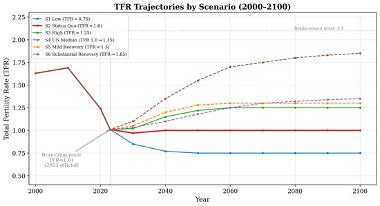
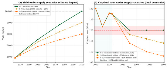
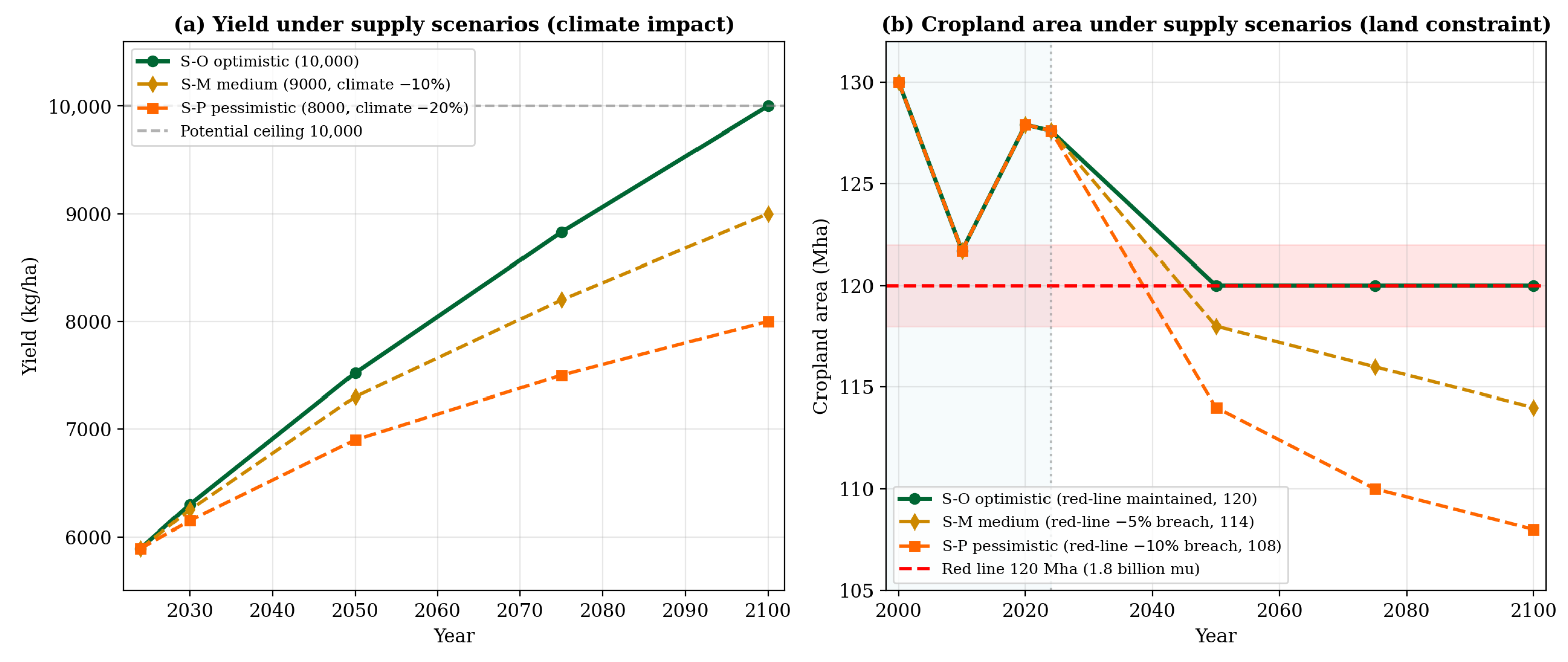
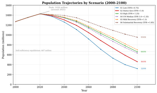
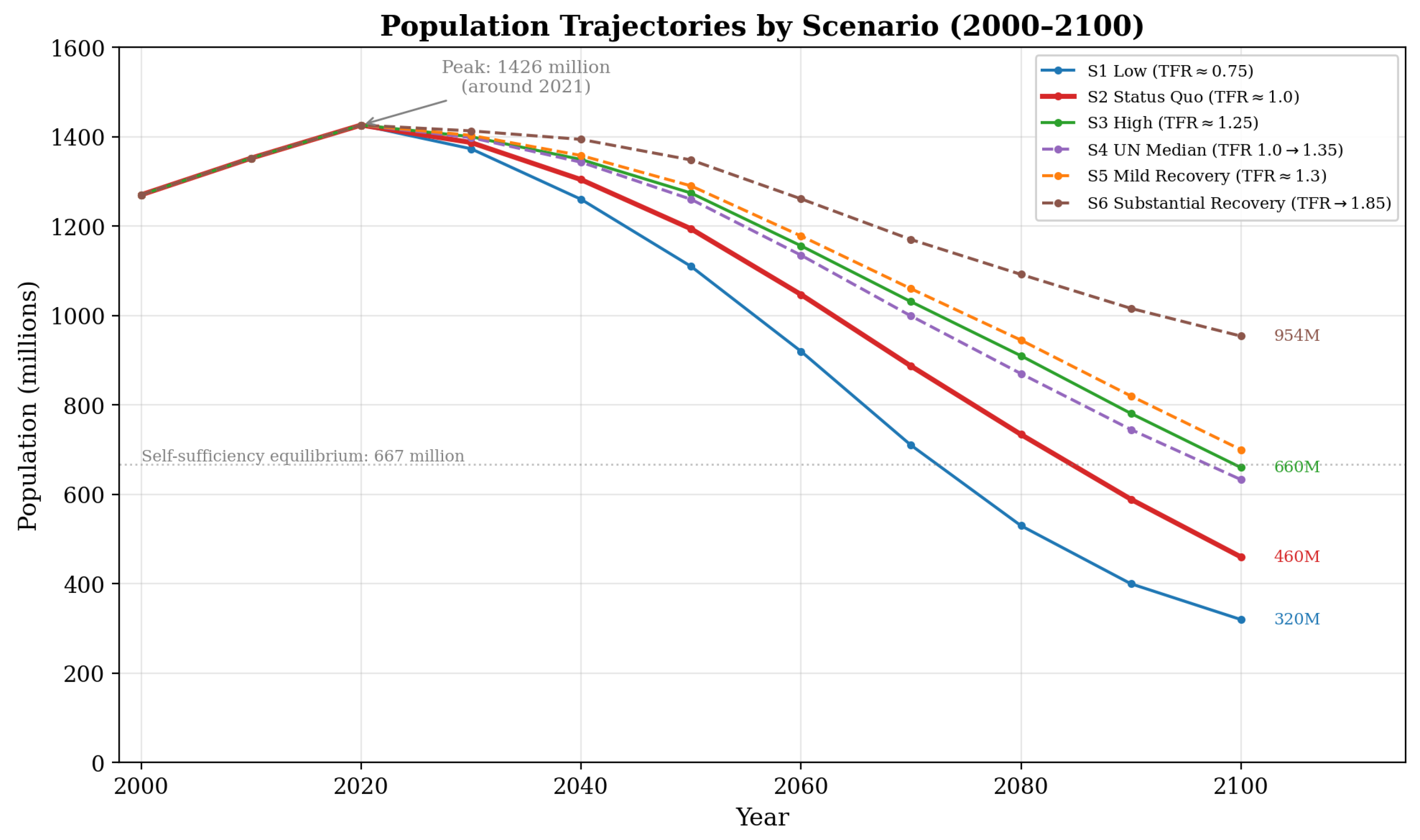
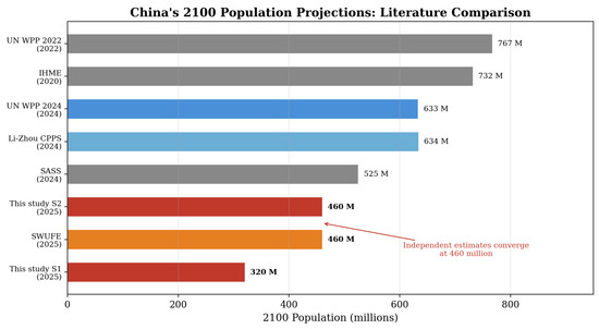
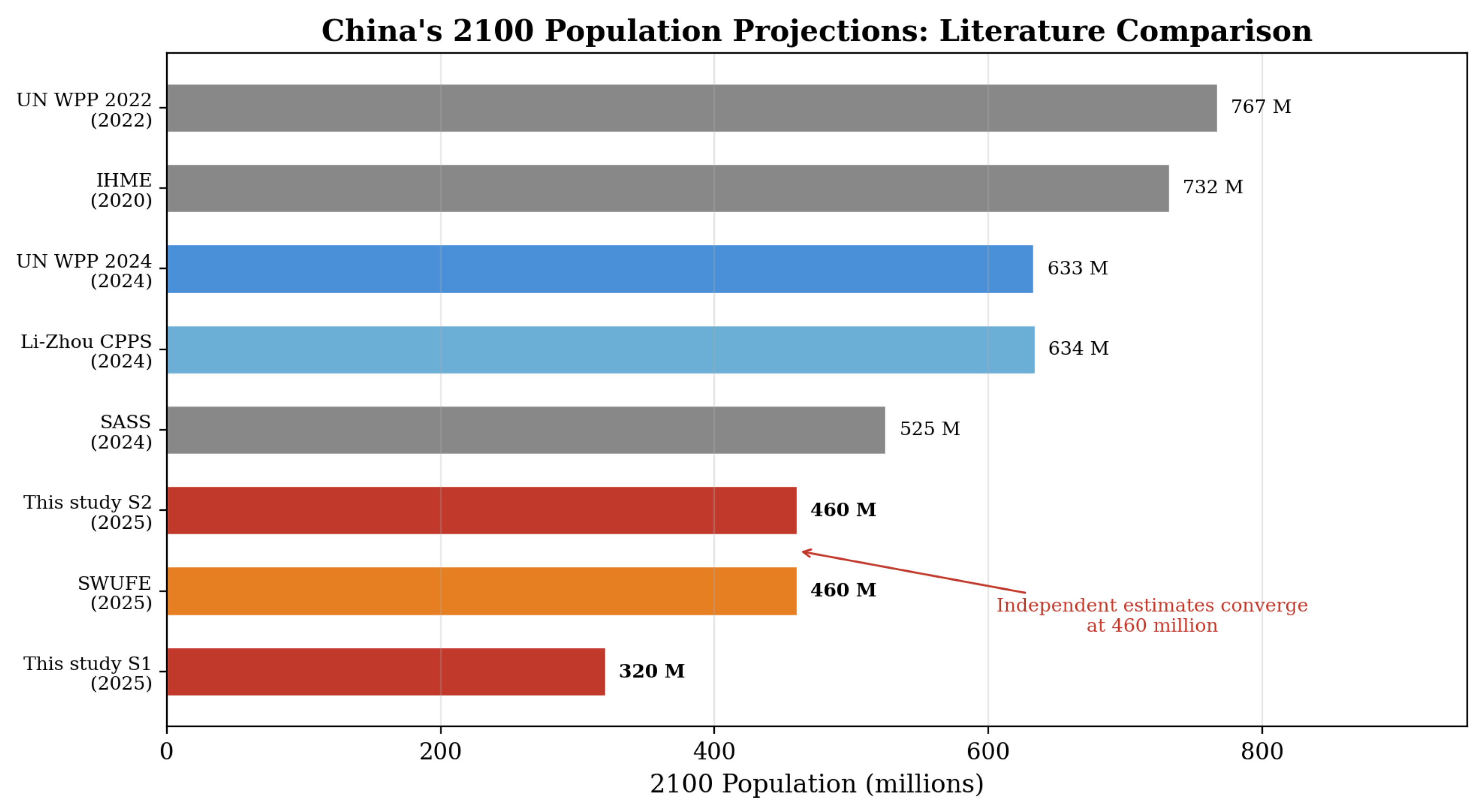
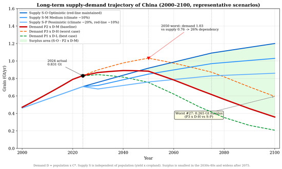
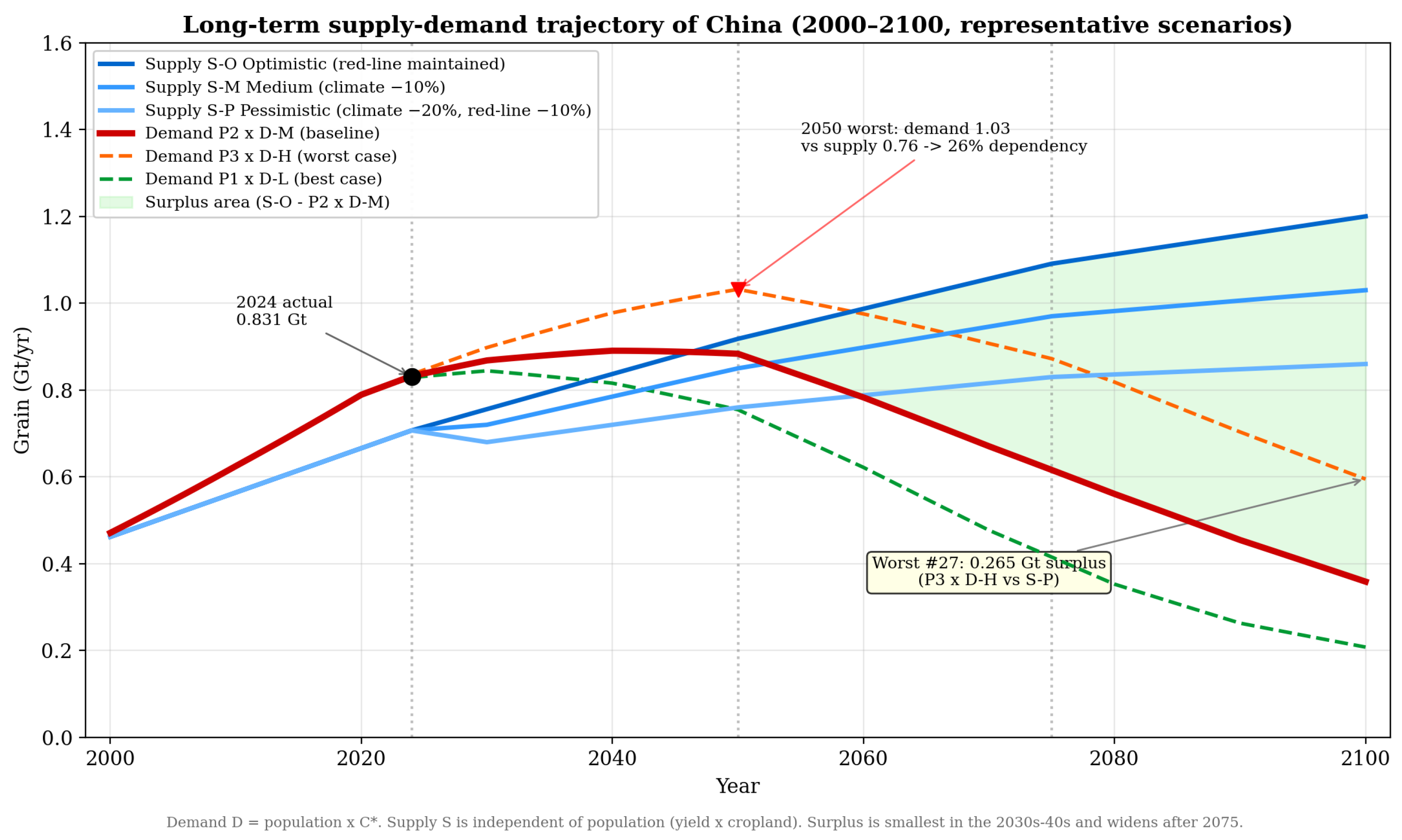
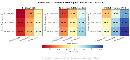
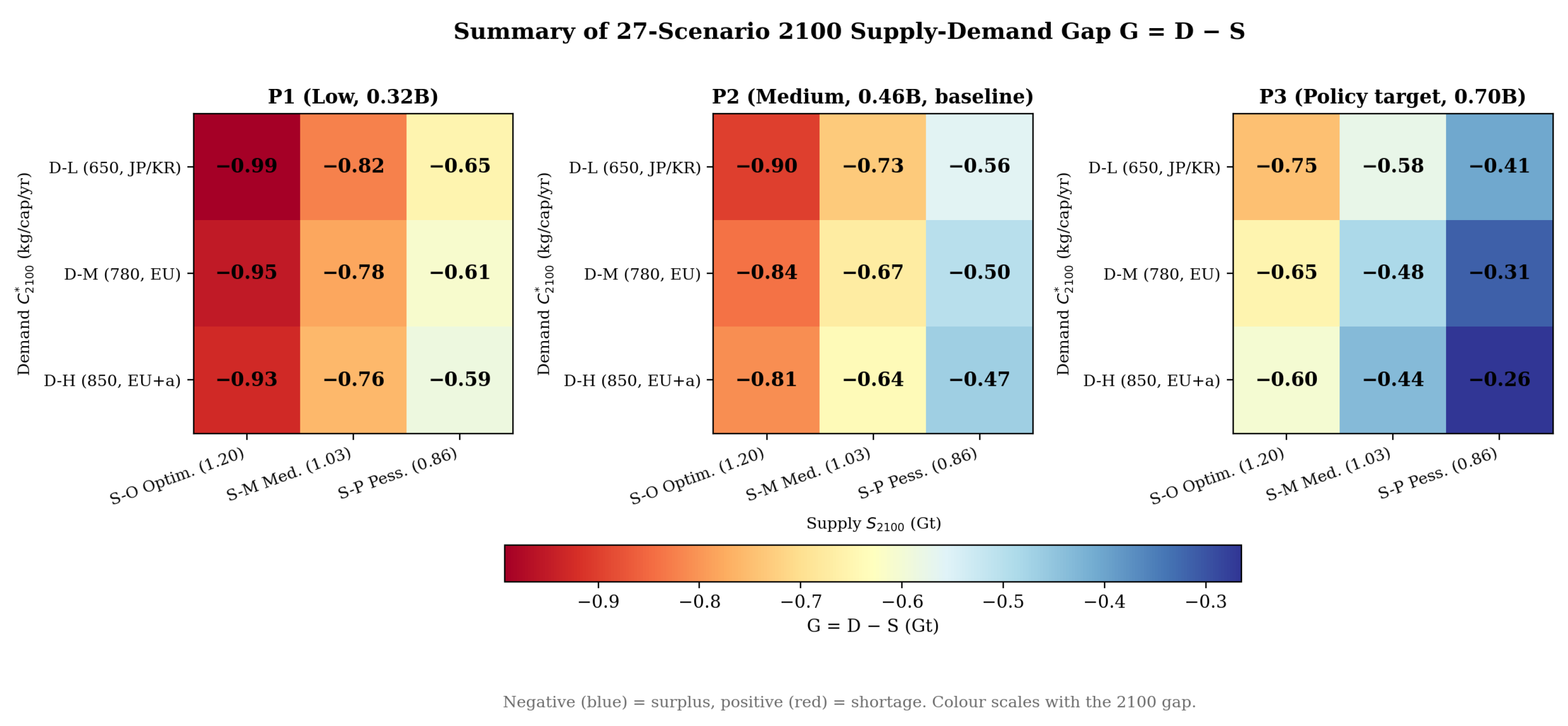
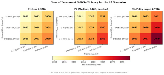
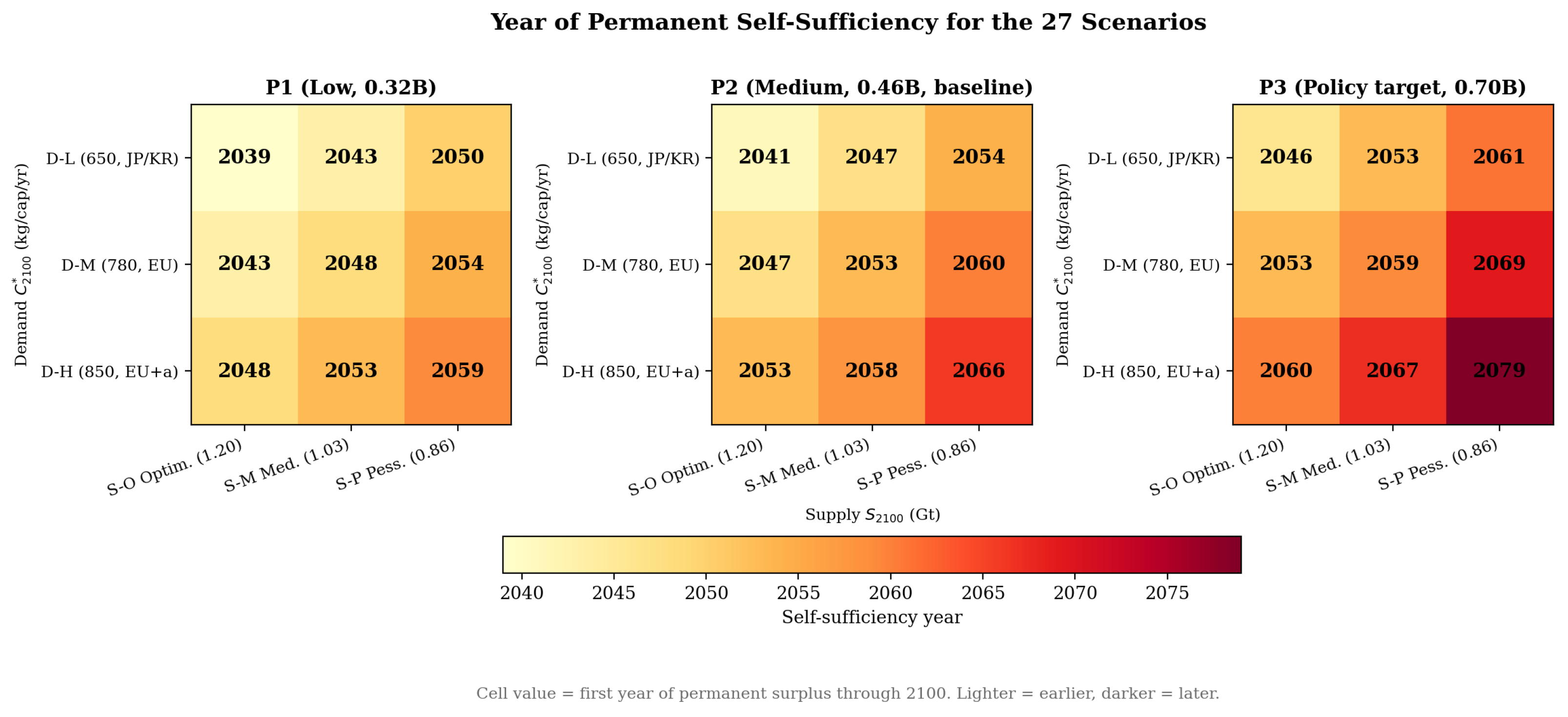
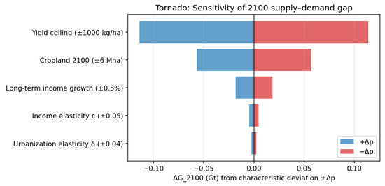
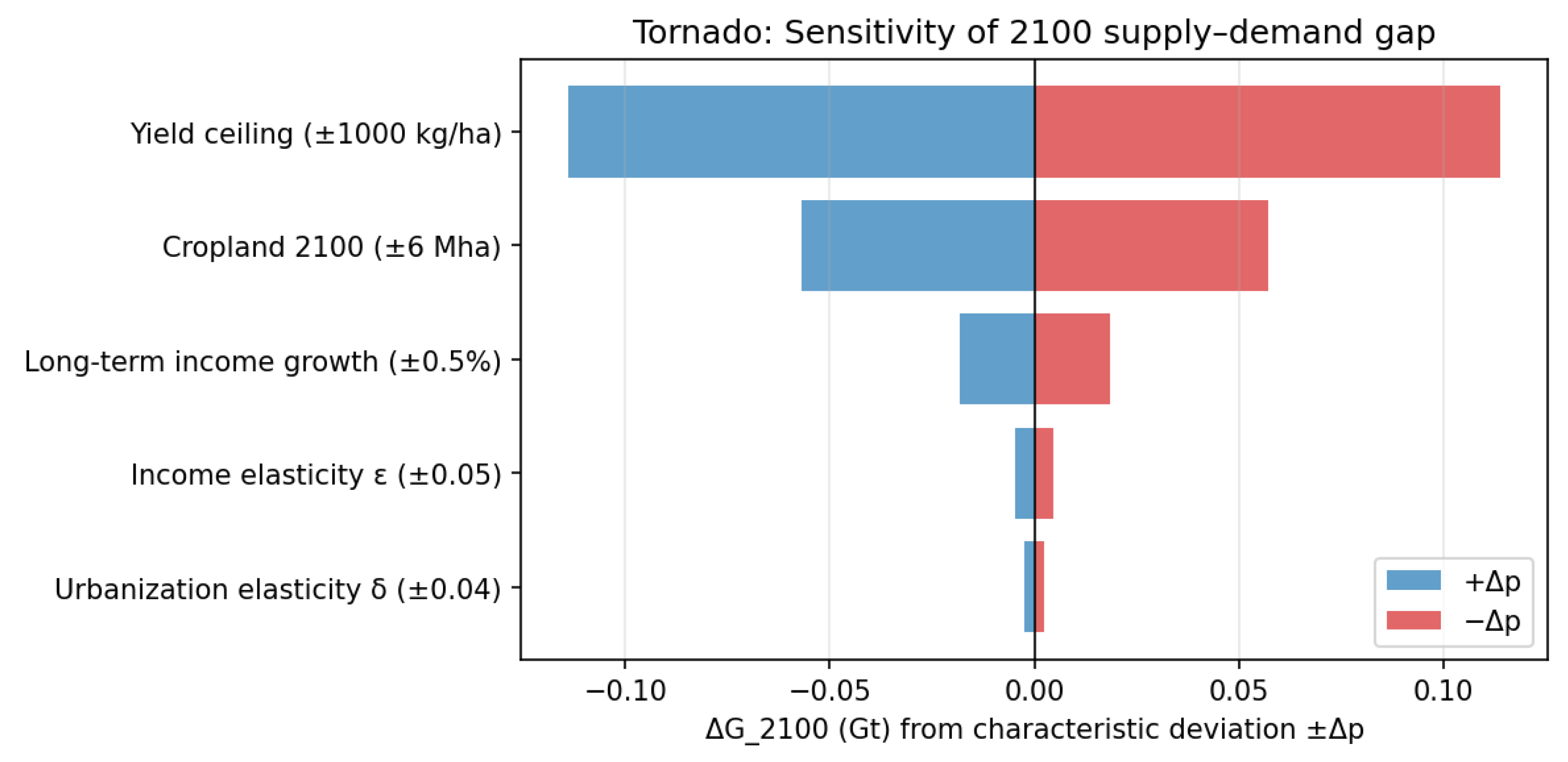

Disclaimer/Publisher’s Note: The statements, opinions and data contained in all publications are solely those of the individual author(s) and contributor(s) and not of MDPI and/or the editor(s). MDPI and/or the editor(s) disclaim responsibility for any injury to people or property resulting from any ideas, methods, instructions or products referred to in the content. |
© 2026 by the authors. Licensee MDPI, Basel, Switzerland. This article is an open access article distributed under the terms and conditions of the Creative Commons Attribution (CC BY) license.