


Abstract
Most Portuguese aquaculture farms are located in estuaries and coastal lagoons, which are highly productive, nutrient-rich transition zones that are also among the most vulnerable to anthropogenic pressures and climate change. This study assesses Ria Formosa’s suitability for grooved carpet shell (Ruditapes decussatus) aquaculture, accounting for projected climate change and a potential increase in clam farming production. The methodology involved implementing a numerical modeling system to map key physico-chemical variables under historical (1995–2014) and future (2081–2100) conditions. Model outputs were then used to compute a suitability index (SI), which was converted into aquaculture suitability maps for this species. Results indicate that the hydrodynamic and transport components reproduced tidal propagation and the transport of salinity and heat effectively. In contrast, simulations of water quality variables were less accurate, reflecting the greater complexity and uncertainty in representing biochemical processes. Across both time periods, environmental conditions were generally less favorable in winter and more favorable in spring. Water temperature and chlorophyll-a concentration emerged as the dominant drivers of seasonal suitability. Projections suggest that Ria Formosa may become increasingly suitable for grooved carpet shell aquaculture by the end of the century. However, expanding production could compromise ecological balance, reduce resilience, and constrain the system’s long-term sustainable development.
1. Introduction
The impacts of climate change, including sea level rise, ocean warming, and changes in precipitation regimes, can directly affect salinity patterns, circulation, extreme events (such as floods, droughts, and storm surges), and water quality (such as eutrophication, harmful algal blooms, and hypoxia) in coastal systems [1,2,3]. Estuaries and lagoons have significant aquaculture potential, as they are highly productive and nutrient-rich environments that support the growth and productivity of aquatic species. However, climate change can cause modifications in the composition and functioning of biological communities [4]. These induced modifications may impact bivalve and fish development, as these species are susceptible to changes in the physical and chemical characteristics of the surrounding water [5,6,7], affecting their abundance and distribution [8].
Aquaculture is one of the most prosperous, but also challenging, activities for the future, considering all the environmental changes expected due to climate change [9,10,11], which has been intensifying over the last few decades, with strong impacts on the environment and human life [12,13]. According to FAO (2022) [10], Portugal has a high consumption of fish products, with an average of 50 kg∙year−1 per capita. The Portuguese aquaculture sector presents enormous potential for growth in the coming years, aiming to achieve a production capacity of 25,000 tons∙year−1 by 2030 [14]. However, this growth may conflict with other natural resource users and economic sectors [15], so it is necessary to identify new areas and/or optimize production in existing areas. Additionally, to ensure ecosystem sustainability while increasing production, it is essential to adopt a holistic perspective on the entire ecosystem rather than focusing solely on the farm scale, incorporating the positive and negative feedback arising from interactions between aquaculture and the surrounding environment into the assessment of ecosystem carrying capacity [16].
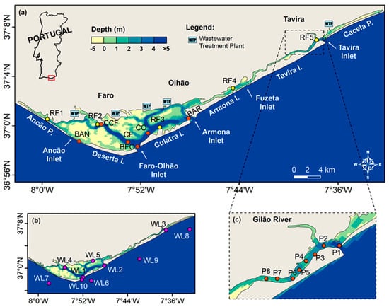
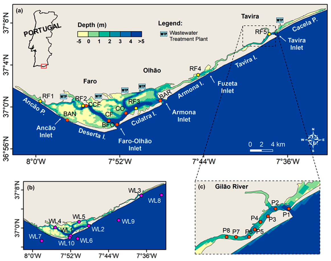
In Portugal, bivalve production represents an important component of coastal aquaculture, particularly in estuaries and coastal lagoons. Among these species, the grooved carpet shell (Ruditapes decussatus) has particular ecological and socioeconomic relevance due to its commercial value and its close dependence on lagoon environmental conditions, including salinity, water temperature, sediment characteristics, water renewal, and food availability. Systems such as Ria Formosa, a coastal lagoon located in southern Portugal (Figure 1), are therefore especially important, as they provide the ecological conditions that support clam growth and production. In this context, the exploitation of grooved carpet shell in managed and licensed growing areas is appropriately framed as aquaculture, whereas harvesting from natural banks should be distinguished as capture fisheries.
Figure 1.
Location and bathymetry of Ria Formosa (a). The sampling stations of water level ((b), purple dots), water temperature and salinity ((a,c), orange dots), water quality properties ((a), yellow dots), and the Wastewater Treatment Plant (WTP) locations are also represented.
The estuarine systems along the continental Portuguese coast present an aquaculture exploitation capacity that has untapped potential for development, which, if duly studied, will allow the identification of new and/or the best areas to be used as aquaculture farms [17,18,19]. It is then essential to leverage current computational resources to develop and apply advanced biogeophysical numerical models that simulate hydrodynamic and biochemical conditions. Hence, this study aims to evaluate the suitability of Ria Formosa for grooved carpet shell aquaculture, taking into account the potential impacts of climate change and the increase in clam production. For this purpose, a 3D model implementation based on the Delft3D model suite was developed and explored to map physico-chemical variables, under present and future conditions. The local water quality and its effects on the development of this shellfish species were analyzed using variables such as water temperature, dissolved oxygen, and chlorophyll-a concentration.
2. Materials and Methods
2.1. Study Area
Ria Formosa is a transgressive barrier island system with unique features located in southern Portugal (Figure 1a). It extends approximately 60 km in the west–east direction from the Ancão peninsula to the Cacela peninsula, respectively, passing through the Deserta, Culatra, Armona, and Tavira islands, separated by Ancão, Faro-Olhão, Armona, Fuzeta, and Tavira inlets (Figure 1a) [20,21]. The lagoon’s average depth is 2 m, and its bathymetry is quite irregular, making water circulation within this coastal system relatively complex [22]. The water exchanges with the ocean are so intense that 50–75% of the total water in the system is renewed with each tidal cycle [23]. The climate is temperate with an annual mean rainfall of around 490 mm [24]. The only small permanent input of freshwater comes from the Gilão river, with an annual mean flow rate of 192 m3∙day−1 [25], despite the existence of other small torrential streams that flow into the lagoon during occasional precipitation events [26]. Therefore, due to the shallow depth, the intense tidal exchange, and the reduced river flow, the system is vertically homogeneous [27].
Ria Formosa is located in an urbanized area surrounded by agricultural lands. Areas such as dunes, lagoon channels, and salt marshes support diverse habitats for several plant, crustacean, bivalve, fish, and bird species of high ecological and economic value [20]. According to the Portuguese Institute for Sea and Atmosphere (IPMA), the lagoon is divided into nine aquaculture zones for bivalve exploitation (https://www.ipma.pt/en/bivalves/index.jsp, accessed on 12 June 2024). Species such as mussels, cockles, oysters, and clams are produced in these aquaculture zones, with the grooved carpet shell accounting for 80% of the national production [25]. This clam species has a high economic value (nearly 16,000 €∙ton−1), representing more than 50% of the total mollusks and crustaceans produced in Portugal [28].
2.2. Model Configuration
The selection of a numerical model must consider the model’s limitations, the processes involved in the study, and the data availability. The numerical model Delft3D, developed by Deltares, is a versatile model that allows the assessment of hydrodynamics, properties, and sediment transport, and water quality in a variety of coastal environments like shallow seas, coastal areas, estuaries, lagoons, rivers, and lakes [29,30,31,32,33].
In this study, a 3D implementation for Ria Formosa was developed using the FLOW and WAQ modules. Detailed information regarding the main configuration settings, boundary conditions, and parameterizations is presented in Table S1. Despite the system exhibiting vertical homogeneity, a 3D model was adopted to fully represent hydrodynamic and transport processes. This choice allows the simulation framework to resolve localized or transient vertical gradients, represent bathymetric and geometric complexities more consistently, and maintain flexibility for conditions in which stratification or vertical variability becomes relevant.
The WAQ simulations were prepared considering different variables and substances that activated several processes, such as the uptake of nutrients derived from algae growth, the nitrification of ammonium, or the calculation of pH (detailed information regarding these processes can be found in Deltares (2021) [34]). This led to 17 physical and chemical process parameters (Table S2) being adjusted during calibration.
Additionally, to describe the uptake and use of energy and nutrients and the consequences for physiological composition throughout an organism’s life cycle, the DEBGRZ grazing module based on the Dynamic Energy Budget (DEB) theory was used [35]. The DEB theory uses an energetic model to describe the rates at which organisms assimilate and utilize energy for metabolic processes such as maintenance, growth, development, and reproduction [36]. This DEB model is based on a generic theory, meaning that the same model structure can be applied to different species with only varying parameter values [37]. The variability in growth and reproduction between individuals of the same species is then mainly caused by differences in environmental conditions, such as water temperature or food availability [38]. The DEBGRZ module can be used for any species or life stage and can describe grazer populations using four state variables: structural biomass, energy, gonadal biomass, and the number of individuals [35].
2.3. Observed Data
Hourly data from a campaign conducted by the Portuguese Hydrographic Institute between October 1979 and October 1980 were used to calibrate the water levels at the WL1–WL9 stations (Figure 1b). The water level validation was performed at WL3, WL4, and WL10 with observed data from the COALA [22,39] and UBEST [24,40] projects.
Water salinity and temperature data from stations BAN, BAR, BFO, CF, and CO (Figure 1a), collected during the COALA project, were used to calibrate the model. Additionally, data from station CCF (Figure 1a) provided by the UBEST project were used for validation. Vertically, the model was validated using vertical profiles of water salinity, temperature, and velocity (stations P1–P7 in Figure 1c) collected during two campaigns (one during the flood and one during the ebb) in September 2022.
Lastly, Chl-a, DO, NH4, NO3, PO4, and SiO4 data from the UBEST project at RF1–RF5 stations (Figure 1a) were used to calibrate the water quality module. At the CCF station, daily average analyses of Chl-a, DO, and pH were conducted from September 2017 to September 2018. For Chl-a, a Butterworth filter with a low-pass band and a cut-off frequency of 1/48 h−1 was applied to remove outliers and high-frequency events from the original 15 min time series [24]. Daily averages were then computed from the filtered series and used in the analysis and comparison with model results. Therefore, the model evaluation for Chl-a was based on the smoothed low-frequency component of the observations rather than on the raw measurements, which should be considered particularly at short timescales.
2.4. Calibration and Validation Procedure
Since numerical models are based on mathematical equations that aim to represent natural processes, their predictions are reliable only if the model assumptions, inputs, and parameter estimates are accurate. The model’s capacity to represent the water systems as accurately as possible is usually evaluated qualitatively by comparing visually model results with observed data, and quantitatively using statistical analysis to measure how model results fit the observed data [41].
Therefore, the Root Mean Square Error (RMSE), the percent Bias (pBias), and the Pearson’s correlation coefficient (R) metrics were determined to quantify the model’s performance. The RMSE evaluates the accuracy of the model’s results by comparing them with the observed values [42], and the pBias expresses the percentual bias between simulated and observed data, quantifying if the model’s results are systematically underestimating or overestimating observations [43]. According to these authors, performance levels can be categorized as excellent (|pBias| < 10%), very good (10% ≤ |pBias| < 20%), good (20% ≤ |pBias| < 40%), and poor (|pBias| ≤ 40%).
For the calibration and validation of the hydrodynamic module, 3D simulations were performed for the periods 15 August 1979 to 30 September 1980, 15 October 2011 to 15 December 2011, and 1 May 2017 to 1 November 2017. A simulation from 1 September to 10 December 2011 was used for calibration of the salt and heat module, and a two-year simulation from January 2017 to January 2019 was used for validation. The water quality was calibrated using results from a single simulation conducted between 2017 and 2018.
2.5. Climate Change and Carrying Capacity Scenarios
Three numerical simulations, representing the historical (1995–2014), the future (2081–2100), and the future with an increase in the clam production quantities (Future + Production), were carried out over 18 months (considering a spin-up of six months) to assess the impacts of climate change and the increase in clam production in Ria Formosa.
For the future period, the results of the most pessimistic greenhouse gas emission scenario (SSP5–8.5) from the 6th Assessment Report of the Intergovernmental Panel on Climate Change [44] were considered. Projections for the end of the century (2100) provide a useful framework for evaluating the long-term consequences of climate change, particularly for sectors that require long planning and investment horizons, such as aquaculture. The inclusion of the 2081–2100 period, therefore, allows stakeholders to assess the system’s response to a strong climate-change signal and to support long-term adaptation, resilience planning, and the development of potential climate policies.
In this context, data from the MPI-ESM1.2 climate model [45], developed by the Max Planck Institute (MPI), was used to study the long-term impacts of climate change. The selection of this model was motivated by its solid performance in reproducing diverse ocean physical and biochemical properties along the Portuguese continental coast [46]. A climatology of oceanic variables (water temperature, salinity, Chl-a, DO, pH, NH4, NO3, PO4, and SiO4) from a grid point near the model’s ocean boundary was computed for the historical and future periods. The MPI model data were then used to calculate the annual-average differences between the two periods. These annual-average differences were computed for the five vertical layers in the model configuration (Table 1) and included in the open-boundary computations based on a climatology of IBI hindcasts for the same historical period (1995–2014). Thus, the future oceanic forcing was constructed using a climatological approach, in which the historical boundary conditions were adjusted by the average end-of-century climate signal derived from MPI-ESM1.2. This approach was adopted to isolate the long-term effect of climate change on the lagoon system, rather than to reproduce the full temporal sequencing of future events. In addition, for the future scenario, a sea level rise of 0.67 m (2081–2100 for SSP5–8.5) was considered [47].
Table 1.
Annual average differences (%) between future and historical MPI (ocean variables) and WRF (atmospheric variables) model results. Layer 0 represents the atmospheric component, and layers 1 (top) to 5 (bottom) the oceanic component.
The atmospheric conditions, both for historical and future periods, were obtained from a high-resolution Weather Research and Forecasting (WRF) model simulation over mainland Portugal, at 6 km horizontal resolution [48,49]. This simulation uses ocean data from the MPI-ESM1.2 model as initial and boundary conditions. Climatologies for the historical and future WRF results were computed after applying a filter to remove atypical values with an occurrence probability lower than 1%. Thus, extreme values (above the 99th percentile) were removed from the climatological analysis to prevent those isolated extreme values from disproportionately influencing the average atmospheric forcing fields, since the purpose of the climatology was to represent the average conditions of each period. Similarly to the oceanic variables, annual average differences between future and historical periods were then calculated for the atmospheric variables (Table 1) and included in an ERA5 climatology for the historical period (1995–2014).
Regarding the river boundary, a 25% reduction in the river discharge obtained from the historical (1990–2020) climatology was applied for the future scenario, considering the Hydrological Research Unit of the Swedish Meteorological and Hydrological Institute (SMHI) projections by the end of the 21st century, for the IPCC’s emission scenario RCP 8.5. Due to data limitations, the concentrations of water quality properties for historical and future scenarios were set equal to those used in the calibration process.
It should be noted that this future forcing strategy is intended to represent average end-of-century conditions and to provide a first-order assessment of changes in environmental suitability under climate change. Thus, it does not preserve the full seasonal evolution, frequency, duration, or sequencing of short-term extreme events, such as heatwaves, intense precipitation, storm episodes, abrupt salinity shifts, or low-oxygen events, which may also affect estuarine aquaculture performance. Consequently, the future suitability estimates presented in this study should be interpreted as reflecting changes in background average conditions.
In addition, the ecological carrying capacity (ECC) of Ria Formosa was evaluated, here defined as the maximum level of use that the system can sustain without irreversible effects on species and ecosystem functioning [50,51]. For this purpose, the Future + Production scenario was used to simulate an increase in clam farming pressure, as this is one of the main economic activities in the lagoon and may expand under future socioeconomic demand. Specifically, the model was initialized with a baseline clam distribution, and clam density was then increased only within the mapped aquaculture farm areas identified by the Portuguese Directorate-General for Natural Resources, Safety and Maritime Services (Figure S1). In these farm areas, density was set to 360 individuals per square meter, equivalent to 86 gC of biomass, based on the methodology of Brito et al. (2023) [52] and on values reported by Duarte et al. (2006) [53] and Ojea et al. (2004) [54], while the remaining lagoon retained the background values. This approach was used to represent an intensification of production in farming zones, rather than a uniform increase across the whole system. This scenario should therefore be interpreted as an intensity case, used to test system sensitivity and ecological limits under increased use of existing farm areas.
2.6. Suitability Index
Aquaculture is one of the fastest-growing production sectors in the world [10], with finfish generally representing a larger share of total production than shellfish [55]. Nevertheless, at the regional level, this may be different. As previously mentioned, the grooved carpet shell is extensively exploited in the nine aquaculture zones of Ria Formosa. Clam farming is usually carried out by planting clam seeds [56]. Shellfish farmers seed their bottom cultures with juvenile clams and harvest them when they reach the commercial size of 25 mm [57]. However, recent studies have revealed that the use of a cultivation method similar to that of the oyster (through structures/cages submerged in the water column) allows clams to grow more and avoid predators and potential pathogens compared to growing underground [58,59,60]. In addition, bivalve aquaculture in open systems requires particular attention because farms interact directly with the surrounding environment and may affect the overall ecosystem dynamics [61,62].
To assess the potential exploitation of the grooved carpet shell in suspended structures in the water column, suitable areas for clam aquaculture in Ria Formosa were identified following the methodology of Pereira et al. (2023) [17]. This approach is based on optimal and minimum/maximum thresholds (Table 2) for key environmental variables, such as water depth, current velocity, water temperature, salinity, Chl-a availability, and good levels of DO and pH controlling clam development [56,63,64].
Table 2.
Environmental optimal and threshold limits for growth and development of the grooved carpet shell.
A relative importance weight is assigned to each environmental variable, except for water depth and current speed, through pairwise comparison using the Analytic Hierarchy Process (AHP). Each variable is converted to a score between 0 and 5. The final Suitability Index (SI) is computed as the weighted geometric mean of the scored environmental variables as described in the following equation:
where is the score of each environmental factor, is the corresponding AHP weight, is the number of each weighted variable, and represents the threshold conditions for water depth and current speed. Whenever falls outside the defined thresholds, a score of 0 is assigned. Finally, suitability for grooved carpet shell aquaculture is classified into five categories: Unsuitable [0–1], Poorly Suitable [1–2], Moderately Suitable [2–3], Very Suitable [3–4], and Highly Suitable [4–5].
Given that the main objective of this study is to evaluate the suitability of the Ria Formosa for the exploitation of the grooved carpet shell, it is crucial to analyze the results by season for the environmental variables (Table 2) that are important for this bivalve, and that enhance and/or hinder its growth. Thus, seasonal averages of water temperature, salinity, Chl-a, DO, and pH were computed for the three scenarios.
3. Results and Discussion
3.1. Model’s Performance
The hydrodynamic model results were compared with water-level data from the WL stations in Figure 1b. The results in Table S3 show the model’s excellent ability to represent the lagoon’s hydrodynamics during the calibration period (1979–1980). At all stations, the RMSE ranged from 5 to 17 cm, with an absolute pBias of 0.3–6.6%. In addition, the achieved R was consistently above 0.99 at all stations. For the validation periods (2011 and 2017), model results highlighted an improvement at station WL4. The RMSE and pBias decreased from 17 cm to 9 cm and from 3.9% to 1.4%, respectively, suggesting that the contemporaneity of the observed data with the bathymetry improved the model’s performance. These results are in line with recent studies in Ria Formosa [25,47,65].
Regarding water temperature and salinity, Table S4 presents the calibration results for the orange stations in Figure 1a. These results indicate that the model consistently and accurately reproduces the patterns of water temperature and salinity in the system. Across all stations, the average salinity is around 36 due to oceanic influence, and the positive pBias indicates a slight overestimation by the model. The BFO station presented the poorest result with an average RMSE of 0.70 and a pBias of 1.95%. For water temperature, model results indicate a slight underestimation at all stations, with the best match between model results and observations at the BAR station, with an average RMSE and pBias of 0.65 °C and −0.84%, respectively. The overall results are very good, with global average RMSE and pBias of 0.44 and 1.05% for salinity, and 1.08 °C and −5.37% for water temperature, which are in line with other studies for this coastal system [25] and others with similar characteristics [17,66].
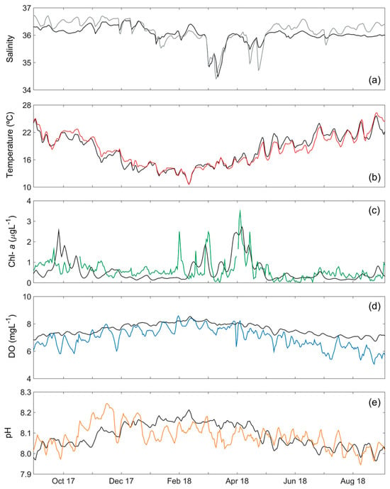
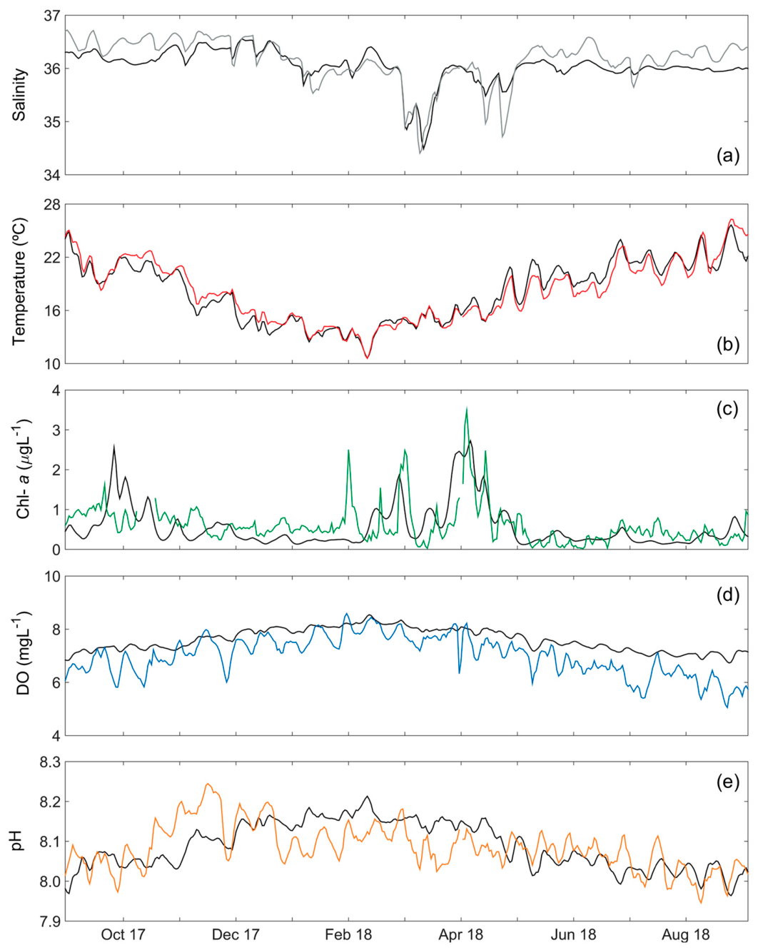
The salt and heat transport module was subsequently validated at the CCF station (Figure 1a). Both the daily average salinity (Figure 2a) and water temperature (Figure 2b) showed a good match between model results and observations, with RMSE and pBias of 0.25% and 0.32% for salinity and 0.94 °C and 0.23% for water temperature. Model results also show strong correlations with observations for both properties (0.85 and 0.96 for salinity and water temperature, respectively).
Figure 2.
Observations (colored lines) and model results (black lines) of daily average salinity (a), water temperature (b), Chl-a (c), DO (d), and pH (e) at the CCF station.
To assess the model performance in reproducing the vertical distribution of water temperature, salinity, and current speed along the water column, vertical profiles of model results and observed data at P1–P8 stations (Figure 1c) were represented. Figure S3 show that the model performs very well in representing the vertical distribution of these properties. At the same time, these figures depict the vertical homogeneity of these variables in the Ria Formosa.
The RF stations presented in Figure 1a were used to calibrate the WAQ module. Table S5 presents the mean (minimum–maximum) of observed and model results for Chl-a, DO, NO3, PO4, SiO4, and NH4 at these stations. Globally, the western stations RF1 and RF2 presented the highest mean, minimum, and maximum differences between observations and model results. In contrast, the eastern stations RF4 and RF5 showed the smallest differences. For maximum Chl-a, RF1 has the highest difference (2.7 µgL−1 data and 0.2 model µgL−1), and RF4 has the lowest (1.0 µgL−1 data and 0.9 model µgL−1). DO is fairly represented across all RF stations, with mean differences of 0.2−0.3 mgL−1. RF2 presents the best and poorest results for PO4 and NO3, respectively. In the first, the minimum (0.1 µM), mean (0.2 µM), and maximum (0.3 µM) concentrations predicted by the model are very close to the observed values. For NO3, the results are not so good. For the other nitrogen compound (NH4), model results were best at the RF1 station (0.3 µM difference between model and data means), and worst at the RF5 station (2.1 µM). The best result for SiO4 was achieved at the RF3 station. These results show that, at most stations, NO3 is overestimated and NH4 is underestimated, suggesting that DIN (NO3 + NO2 + NH4) is well represented by the model.
Additionally, model results were also compared with observations of Chl-a, DO, and pH at the CCF station (Figure 2c–e). Similar to the results obtained for water temperature and salinity, the results at this station were very good. The Deflt3D model simulated the Chl-a pattern over one year (September 2017–September 2018) with an RMSE of 0.5 µgL−1, a pBias of 8.8%, and an R of 0.5. DO and pH were also satisfactorily reproduced by the model (with correlations of 0.8 and 0.5, respectively). The model results showed a slight overestimation (pBias of −8.5% for DO and −0.3% for pH), with RMSE of 0.7 mgL−1 and 0.06 for DO and pH, respectively. The lack of water quality observations throughout the water column prevents calibration and validation of the model’s vertical structure.
These findings align with those reported in other studies conducted in two different systems [67,68]. Mendes et al. (2021) [67] obtained an RMSE of 1.02 mgL−1 for DO in a modeling study at the Mondego estuary, and Wang et al. (2017) [68] obtained an average RMSE of 12 µgL−1 at Breton Sound estuary. The 12 µgL−1 error is much higher than the mean error in this study (0.5 µgL−1). However, at the Breton Sound estuary, the Chl-a concentration ranges from 0 to 40 µgL−1, which means that an error of 12 µgL−1 represents approximately 30% of the total variation. In Ria Formosa, at the CCF station, Chl-a varies from 0 to 3 µgL−1 (Figure 2c), meaning that an RMSE of 0.5 µgL−1 represents 17% of the total variation in this property.
Compared with Rodrigues et al. (2021) [25], a modeling study in Ria Formosa carried out with a different numerical model (SCHISM) using the same RF observations, the results are of the same order. According to Mateus et al. (2012) [69] and Vaz et al. (2015) [70], nutrient unpredictability and the lack of good load data are important limitations in water quality modeling, which means that collecting in situ continuous data (both spatial and vertical) is of utmost importance to address these limitations and enhance the model’s performance.
3.2. Historical and Future Spatial Patterns
3.2.1. Historical vs. Future
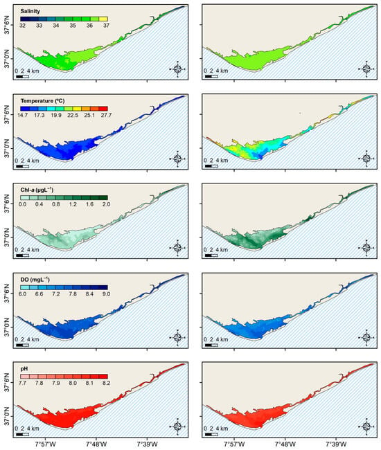
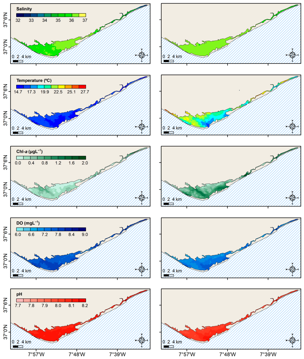
By analyzing the patterns of water temperature, Chl-a, and DO in Figure 2, spring (April, May, and June) was selected as the best season for aquaculture exploitation, and winter (January, February, and March) was the least favorable. In this context, horizontal maps of the historical (1995–2014) average salinity, water temperature, Chl-a, DO, and pH for winter and spring are shown in Figure 3.
Figure 3.
Maps of the historical (1995–2014) average salinity, water temperature, Chl-a, DO, and pH for the winter (left panel) and spring (right panel).
For winter conditions, water temperature ranges between 14.7 and 17.3 °C and salinity between 33 and 36 throughout the lagoon. The eastern part of the lagoon exhibits low salinity levels due to the Gilão River’s discharge within this region. The west and central parts of the lagoon are dominated by oceanic waters. According to Brito et al. (2010) [71], occasional strong rainfall events can also affect the lagoon’s salinity. The concentration of Chl-a in the water column presents its lowest levels, not exceeding 0.4–0.6 µgL−1. In contrast, DO reaches its maximum concentration (9 mgL−1). DO solubility is affected by water temperature, pressure, and salinity [72]. Ocean waters generally have 20% less DO than freshwater at the same temperature [73]. During the winter season, when the water temperature is low, the lagoon presents the highest DO contents (Figure 2). The pH of around 8 shows the influence of oceanic waters in this system.
For spring conditions, a homogeneous salinity of 36.5 is observed in the entire lagoon. According to the Venice system classification [74], Ria Formosa can be classified as a Euhaline system during the winter and spring seasons. The water temperature is higher in spring than in winter, reaching 24 °C in the innermost regions due to increased solar radiation. During this milder season, the highest Chl-a concentrations (2 µgL−1) are found since physicochemical parameters, such as water temperature, contribute directly to increasing the Chl-a content in the water [52,75]. These concentrations in the water column are within the range previously found by Falcão and Vale (2003) [76] and Newton et al. (2003) [77]. However, other processes, such as the resuspension of the surface part of the large benthic algal community, can affect these concentrations [71]. According to Brito et al. (2012) [78], several European coastal lagoons exhibit low pelagic but high benthic Chl-a concentrations. The DO concentration is lower in spring (7.2−7.8 mgL−1) than in winter as a result of the increase in water temperature, and the pH (approximately 7.9) is also slightly lower.
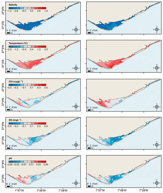
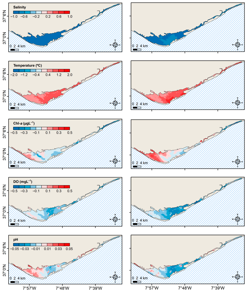
After analyzing the historical period, the possible impacts of climate change in the lagoon were assessed by comparing differences in salinity, water temperature, Chl-a and DO concentrations, and pH between the future (2081–2100) and historical (1995−2014) scenarios for the winter and spring seasons. These differences are depicted in Figure 4.
Figure 4.
Differences between future (2081–2100) and historical (1995–2014) conditions for the average salinity, water temperature, Chl-a, DO, and pH during winter (left panel) and spring (right panel).
Regarding winter, the model predicts a general decrease in salinity (around 1.0) and an increase in water temperature (up to 1.2 °C) throughout the lagoon. The concentration of Chl-a is expected to increase (around 0.3 µgL−1) on the west side of the lagoon and to decrease (around −0.3 µgL−1) on the east side, despite the increase in water temperature and Chl-a concentration at the oceanic boundary (approximately 6% of the average water column). A slight reduction in DO (approximately −0.4 mgL−1) and a negligible variation in pH (between −0.01 and 0.01) are expected in the future. In spring conditions, the differences predicted in winter persist but may be more pronounced. The model predictions show an increase in water temperature of approximately 1.5 °C, a decrease in DO of up to −0.5 mgL−1, and an acidification (lower pH) of 0.05. These results might also be linked to the predicted sea-level rise, which will induce non-linear effects in the lagoon’s hydrodynamics due to its complex shape and configuration [65].
3.2.2. Historical vs. Future + Production
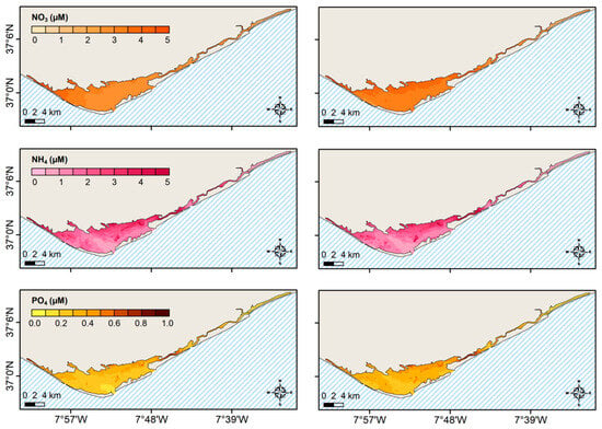
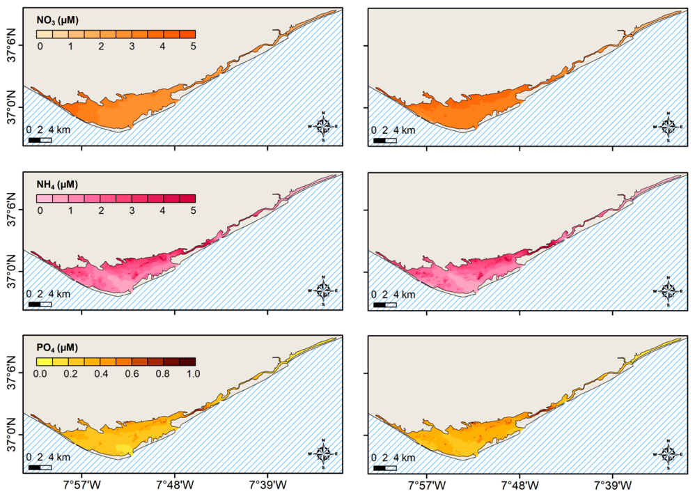
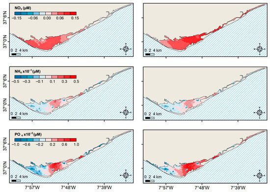
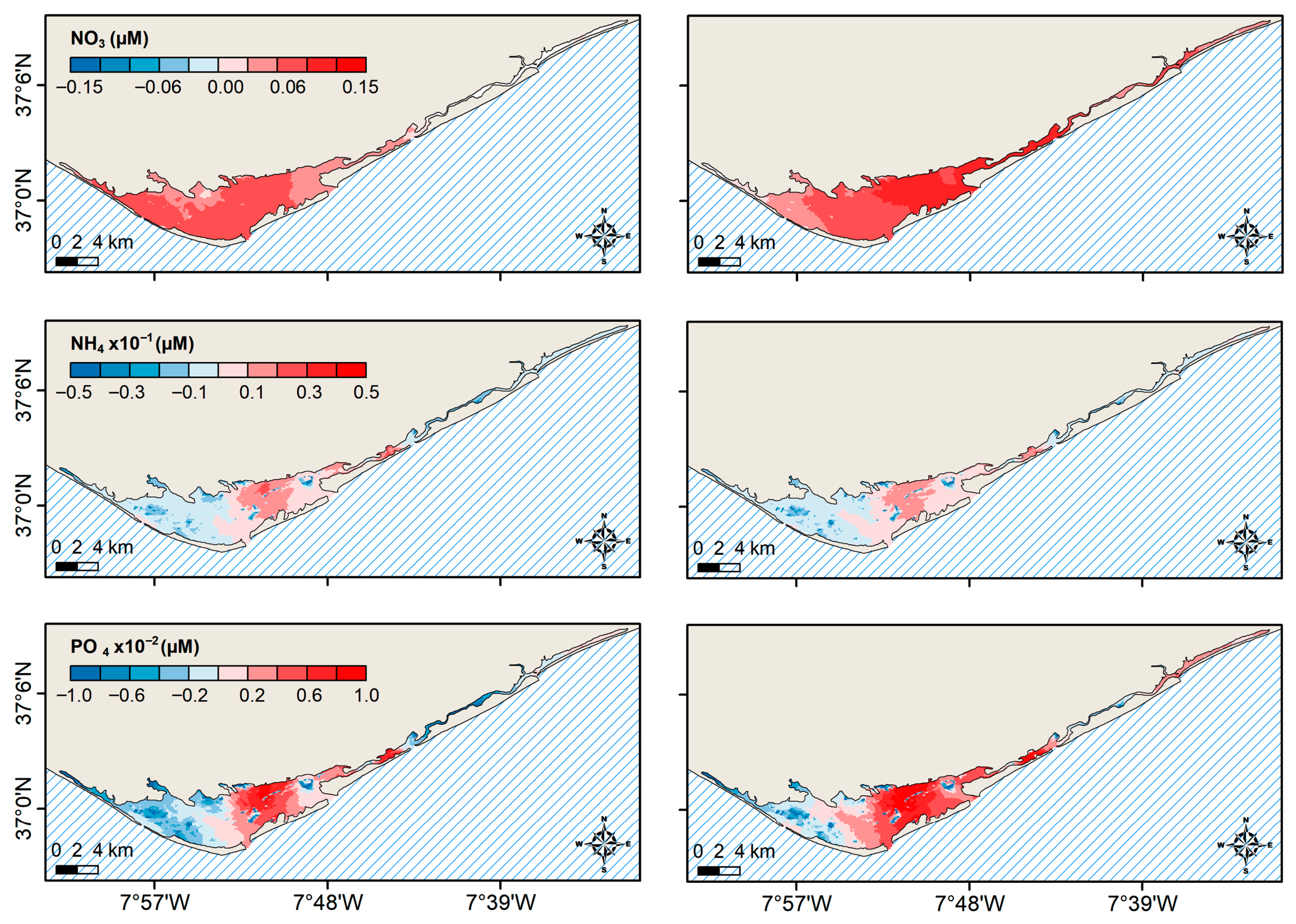
Considering the future scenario with an increase in clam production, additional maps of the main nutrients (NO3, NH4, and PO4) for the historical (1995–2014) period were represented due to the effect of increased production quantities on abiotic factors [52]. Figure 5 shows the spatial distribution of these variables for winter and spring. The results for both winter and spring show a homogeneous system with average concentrations along the lagoon of 3–4 µM for NO3, 1–5 µM for NH4, and 0.2–0.8 µM for PO4. In the future (2081–2100) scenario with increased production quantities (Figure 6), the greatest impacts are observed near the farm areas (Figure S1). In both winter and spring, the differences in NO3, NH4, and PO4 concentrations show an increase close to the aquaculture farms, possibly due to the clams’ physiological activity.
Figure 5.
Maps of the historical (1995–2014) average NO3, NH4, and PO4 for the winter (left panel) and spring (right panel).
Figure 6.
Differences between future (with increased production) and historical (1995–2014) conditions for the average NO3, NH4, and PO4 during winter (left panel) and spring (right panel).
Generally, an increase in clam production may result in some changes in the lagoon, especially at the local scale. Also, an increase in the clam’s biomass may have additional implications for the phytoplankton community’s structure. Nevertheless, the effective impact of these changes on the community composition and the ecological role of phytoplankton is not fully understood.
3.3. Suitability Maps
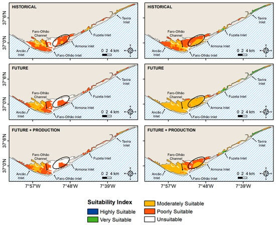
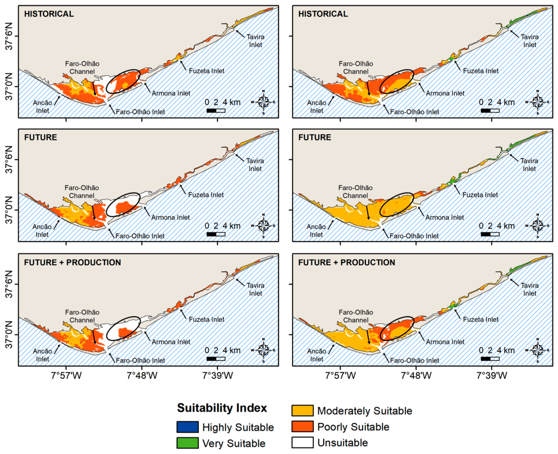
The Ria Formosa’s suitability maps for grooved carpet shell exploitation in winter and spring are shown in Figure 7. In general, model results suggest that the majority of the lagoon is considered suitable for the exploitation of this species. However, this suitability is moderate or poor. The areas near the inlets and in the Faro-Olhão channel are considered unsuitable, mostly due to the high current speeds there. Duarte et al. (2020) [79] used three hydrodynamic indicators (average current velocity, maximum flood current velocity, and residence time) to define the best location for shellfish beds in this coastal lagoon. Results showed that in suitable areas, the average current velocity ranged from 0.09 to 0.10 m∙s−1, the maximum flood current velocity was 0.20 m∙s−1, and the residence time was less than 2 days. In another Portuguese coastal shallow lagoon (Ria de Aveiro), Vaz et al. (2021) [19] concluded that bivalve aquaculture is mainly limited by local geomorphology and hydrodynamic characteristics, such as unsuitable current velocities.
Figure 7.
SI maps for the exploitation of the grooved carpet shell in Ria Formosa during winter (left panel) and spring (right panel), considering historical, future, and future + production scenarios. The black ellipse shows the location of the majority of clam farms in the lagoon.
For winter, the historical SI map shows poorly suitable conditions for the exploitation of the grooved carpet shell in the majority of the system. Nevertheless, there is a region north of the Faro-Olhão inlet that has unsuitable conditions. The physical properties presented in Figure 3 and the annual patterns in Figure 2a,b are in the range of the thresholds for the suitability of grooved carpet shell exploitation. The mean water temperature and salinity range are 14–17 °C and 35–36, respectively, and the thresholds of this clam species are 2–30 °C for water temperature and 15–40 for salinity (Table 2). DO also does not represent a limitation to the system’s suitability, since its seasonal average (Figure 3) and yearly concentrations between 7 and 8 mgL−1 (Figure 2d) are within the optimal range for this property (5–8 mgL−1). The same is true for pH (Figure 2e and Figure 3).
Apparently, the Chl-a concentration is mainly responsible for the low suitability levels of the lagoon for the exploitation of the grooved carpet shell. Figure 2c shows the annual variation in Chl-a at the CCF station located in the Faro-Olhão channel. An average Chl-a concentration in the water column of approximately 1 µgL−1 is observed. Analyzing the thresholds for Chl-a presented in Table 2, it can be seen that this average concentration falls within the minimum limit for the growth and development of the grooved carpet shell. The map of Chl-a concentration in Figure 3 shows most of the system with concentrations between 0.2 and 0.8 µgL−1. These low levels of Chl-a concentration are a consequence of tidal exchange and low residence times [30,80]. In fact, due to tidal exchange, a wide variation in water variable concentration can be found in shallow lagoons between flood and ebb [71]. These results are in agreement with the findings of Picado et al. (2023) [18] that studied another coastal system (Ria de Alvor) close to Ria Formosa. These authors found a parallel result for the exploitation of two different bivalve species (Crassostrea angulata and Mytilus spp.) using a methodology similar to that used in this study.
In spring, compared to winter, the water temperature increases (16–22 °C), and the salinity remains at 36 (Figure 2b and Figure 3). The increase in water temperature improves the suitability index, as these limits fall within the optimum thresholds shown in Table 2. Concerning DO and pH, the variations from winter to spring are not significant enough to change the SI classification. Finally, with the increase in Chl-a available in the water column, there is a positive effect on the lagoon’s suitability for clam aquaculture. According to Figure 2c and Figure 3, the average Chl-a concentration ranges from 1 to 2 µgL−1, which falls within the optimal range (Table 2). This increase in Chl-a concentration also makes the area on the east side of the Tavira inlet very suitable.
Nevertheless, the high productivity of Ria Formosa supports complex food webs with different food sources available [81]. Bivalves are known for their capacity to select food based on particle size and food quality [82]. Benthic micro-algae biomass (microphytobenthos), which represents 99% of the total micro-algae chlorophyll biomass of the system, can contribute up to 25% to the chlorophyll found in the water column through resuspension [71,83]. This resuspension close to the bottom only seems to occur at the beginning of the flood tide [30].
Therefore, sediment–water exchanges are very important in the lagoon’s nutrient dynamics [71]. In shallow enclosed coastal systems like Ria Formosa, a large volume of water spreads over a large area, and the sediments present there are of great importance [84]. According to Brito et al. (2010) [71], depending on environmental conditions such as salinity, water temperature, and dissolved oxygen, sediments can act as sources or sinks of nutrients, thereby affecting water quality. The main sources of nutrients in the lagoon are point source discharges, sediment nutrient release, and the run-off from fertilized areas [83]. Due to insufficient data and required inputs, this implementation did not account for exchanges between the water column and the lagoon’s bottom. Future studies should address this limitation.
In the future (2081–2100) scenario, for winter and spring, the system’s suitability slightly increases, mainly in the middle part of the lagoon (Figure 7—middle panel). This is mostly due to an increase in the water temperature (Figure 4). Near the farms’ region, due to increased production (Future + Production scenario in Figure 7), a decrease in the SI is predicted. The increase in production volume leads to lower levels of Chl-a and DO in regions near aquaculture farms [52]. Additionally, with increased production, clams’ higher physiological activity leads to nutrient enrichment. In Figure 6, this effect is noticeable with increases in NH4 and PO4 in the region near the aquaculture facilities.
In a study conducted by Duarte et al. (2006) [53], the authors used the EcoDynamo model [85] to examine scenarios of grooved carpet shell cultivation densities, improvements in wastewater treatment performances, and changes in bathymetry due to dredging operations. These authors found that increasing bivalve densities in farm areas may lead to declines in water quality and reduced bivalve growth due to food limitations. They also reported increases in ammonium and decreases in Chl-a concentrations when biomass density was doubled relative to the base density, consistent with this study’s results.
Regarding the study’s limitations, one source of uncertainty arises from the use of calibration and validation datasets collected at different times. Since the available observations span several decades, they may reflect distinct environmental conditions and, potentially, bathymetric or morphological changes in the lagoon. This limitation is particularly relevant in dynamic coastal systems such as Ria Formosa, where inlet configuration and shallow areas may evolve over time. Consequently, the model assessment should not be interpreted as a reproduction of a single, fully consistent historical state, but rather as an evaluation of the model’s ability to represent the dominant hydrodynamic and water quality processes of the system.
The interpretation of the SI should also account for the uncertainty associated with the model simulations. Since SI is derived from modeled environmental conditions, its reliability depends on the accuracy of the underlying hydrodynamic and water quality simulations. In the present study, hydrodynamic variables were reproduced more accurately than some of the water quality variables. As these variables directly contribute to the SI calculation, uncertainty in their simulation propagates into the final suitability scores and may influence the class assigned to a given location, especially when SI values are close to class boundaries. Nevertheless, as SI is calculated on a seasonal basis and integrates conditions over extended periods, the influence of short-term fluctuations and random model errors is reduced. In addition, the weighted geometric mean used within the AHP framework limits the dominance of any single variable, supporting a more balanced assessment. Therefore, the SI maps presented in this study should be interpreted primarily as indicators of the main spatial and seasonal patterns of suitability, with greater confidence in areas where suitability is consistently high or low, and with more caution in transitional areas where classification may be sensitive to model error.
Another important limitation of this study is that projections for distant future periods, such as 2081–2100, cannot be directly validated. Therefore, future simulations should be interpreted as scenario-based projections of the system response under projected climate forcing, rather than as deterministic forecasts. Confidence in these results relies on the model’s skill under current hydrodynamic and water quality conditions, assuming that the main physical and biogeochemical processes remain adequately represented under future forcing. However, uncertainty increases with the projection horizon, since long-term environmental change may involve nonlinear responses, altered boundary forcings, and ecological shifts that are not fully captured by the current model framework.
An additional source of uncertainty is related to the river boundary conditions adopted in the future scenarios. Due to the lack of reliable projections of future riverine water quality and nutrient concentrations, values at the river boundary were kept equal to those used in the calibration simulations. This assumption may bias future projections since climate change, land-use change, and watershed-scale adjustments may significantly modify freshwater quality inputs to the lagoon. As a result, future nutrient enrichment, phytoplankton biomass, and dissolved oxygen dynamics may be underestimated or overestimated. However, in the case of Ria Formosa, the fluvial contribution is relatively small compared with oceanic exchange and is expected to remain low under future conditions. Consequently, the projected changes should be interpreted as the response of the lagoon to altered climatic and oceanic forcing, rather than as a fully coupled watershed–lagoon future forecast.
4. Conclusions
This study presented a comprehensive assessment of the suitability of the Ria Formosa for the exploitation of grooved carpet shell using numerical hydrodynamic and water quality models. The model results showed very good qualitative and quantitative agreement with observations of water level, water temperature, salinity, and Chl-a, but lower accuracy for DO, pH, and nutrients. The good model performance enabled the study of 3 scenarios: historical (1994–2005), future (2081–2100), and future (2081–2100) with increased production quantities.
Model results suggest that the lagoon presents suitable conditions for clam aquaculture, though the suitability is of a moderate or poor level. For winter, the SI map for the historical conditions shows that most of the lagoon exhibits poorly suitable conditions for grooved carpet shell cultivation. Results also suggest that water temperature and Chl-a concentration are the main variables affecting this outcome. In the future, an increase in the lagoon’s suitability, mainly in the central area, is predicted by the model, especially due to an increase in the water temperature. However, the central-east and eastern areas of the lagoon will be significantly impacted by climate change, as Chl-a and DO concentrations decrease. The increase in production quantities is expected to further reduce DO and Chl-a concentrations, deteriorating water quality near farm areas and, consequently, decreasing the system’s suitability. Additionally, increased physiological activity in the clams may increase nutrient levels, such as NH4. These findings highlight the need to consider the environmental implications of intensified aquaculture.
The intensified production scenario indicates the potential for ecological imbalance under increased farming pressure. However, this feedback is only partially represented in the present model. While the modeling framework explicitly resolves the main hydrodynamic and biogeochemical responses to increased biomass, broader ecological feedbacks, such as indirect trophic effects, long-term ecosystem reorganization, and adaptive responses, are considered conceptually rather than modeled explicitly. Thus, the results should be interpreted as evidence of increasing system stress and possible carrying-capacity limits, rather than as a full representation of all ecological consequences of intensified production.
Future studies should focus on developing strategies for the sustainable intensification of aquaculture practices in Ria Formosa, while accounting for the ecological and environmental consequences of increased clam farming. This involves innovative approaches to maintain water quality, optimize production methods, minimize environmental impacts, ensure ecological balance, and support sustainable growth in clam farming.
Supplementary Materials
The following supporting information can be downloaded at: https://www.mdpi.com/article/10.3390/sci8050100/s1, Figure S1. Location of the current clam farms (in orange) at the Ria Formosa. Figure S2. Vertical profiles of model results (dashed lines) and observed data (solid lines) for salinity (red color), water temperature (blue color), and current speed (black color) at P1–P8 stations (Figure 1c) during ebb. Figure S3. Vertical profiles of model results (dashed lines) and observed data (solid lines) for salinity (red color), water temperature (blue color), and current speed (black color) at P1–P8 stations (Figure 1c) during the flood. Table S1. Description of the main configuration settings, boundary conditions, and parameterizations. Refs. [86,87,88,89,90] are cited in Table S1. Table S2. Description and values of the process parameters used in the WAQ model. Values adapted from Kaçıkoç & Beyhan (2014) [31], Zijl et al. (2021) [33], Deltares (2021) [34], Brito et al. (2023) [52], and Wang et al. (2017) [68]. Table S3. RMSE and pBias from the comparison between model results and observed water level. Table S4. RMSE and pBias resulted from the comparison between model results and observed salinity and water temperature. Table S5. Mean (minimum and maximum) of model results and observed data for Chl-a, DO, NO3, PO4, SiO4, and NH4 at RF1–RF5 stations.
Author Contributions
Conceptualization, H.P., A.P. and J.M.D.; methodology, H.P., A.P. and J.M.D.; software, H.P., A.P. and D.C.; validation, H.P., A.P., I.A., A.C.B. and J.M.D.; formal analysis, H.P. and A.P.; investigation, H.P.; resources, J.M.D.; writing—original draft preparation, H.P.; writing—review and editing, A.P., I.A., M.C.S., A.C.B., D.C. and J.M.D.; visualization, H.P. and A.P.; supervision, A.P., I.A. and J.M.D. All authors have read and agreed to the published version of the manuscript.
Funding
This work was funded by national funds through FCT—Fundação para a Ciência e a Tecnologia I.P., under the project CESAM—Centro de Estudos do Ambiente e do Mar, with references UID/50017/2025 (doi.org/10.54499/UID/50017/2025) and LA/P/0094/2020 (doi.org/10.54499/LA/P/0094/2020). FCT also funded David Carvalho with a researcher contract (CEECINST/00013/2021/CP2779/CT0017), and Ana C. Brito through the Scientific Employment Stimulus Programme (CEECIND/00095/2017).
Data Availability Statement
The data presented in this study are available from the corresponding author upon reasonable request.
Acknowledgments
The authors acknowledge the support of the project CESAM—Centro de Estudos do Ambiente e do Mar, and FCT—Fundação para a Ciência e a Tecnologia I.P. for the research grants. The authors also thank the ClimACT project (2022.01896.PTDC), the strategic project UIDB/04292/2020 awarded to MARE, and the LA/0069/2020 project granted to the Associate Laboratory ARNET. This work also benefited from the infrastructure CoastNet (PIN-FRA/22128/2016). The authors also acknowledge the support from the Xunta de Galicia under project ED431C 2021/44 (Grupos de Referencia Competitiva), the Agencia Estatal de Investigación, and the European Union NextGenerationEU under projects PID2021-125060OB-I00 and TED2021-129756B-C31.
Conflicts of Interest
The authors declare no conflicts of interest.
Abbreviations
The following abbreviations are used in this manuscript:
| AHP | Analytic Hierarchy Process |
| Chl-a | Chlorophyll-a |
| DEB | Dynamic Energy Budget |
| DO | Dissolved Oxygen |
| ECC | Ecological Carrying Capacity |
| IBI | Iberia-Biscay-Ireland |
| IPMA | Portuguese Institute for Sea and Atmosphere |
| MPI | Max Planck Institute |
| SI | Suitability Index |
| SMHI | Swedish Meteorological and Hydrological Institute |
| WRF | Weather Research and Forecasting |
| WTP | Wastewater Treatment Plant |
References
- Filgueira, R.; Guyondet, T.; Comeau, L.A.; Tremblay, R. Bivalve Aquaculture-Environment Interactions in the Context of Climate Change. Glob. Change Biol. 2016, 22, 3901–3913. [Google Scholar] [CrossRef] [Scilit]
- Leal Filho, W.; Nagy, G.J.; Martinho, F.; Saroar, M.; Erache, M.G.; Primo, A.L.; Pardal, M.A.; Li, C. Influences of Climate Change and Variability on Estuarine Ecosystems: An Impact Study in Selected European, South American and Asian Countries. Int. J. Environ. Res. Public Health 2022, 19, 585. [Google Scholar] [CrossRef] [Scilit]
- Robins, P.E.; Skov, M.W.; Lewis, M.J.; Giménez, L.; Davies, A.G.; Malham, S.K.; Neill, S.P.; McDonald, J.E.; Whitton, T.A.; Jackson, S.E.; et al. Impact of Climate Change on UK Estuaries: A Review of Past Trends and Potential Projections. Estuar. Coast. Shelf Sci. 2016, 169, 119–135. [Google Scholar] [CrossRef] [Scilit]
- Cardoso, P.G.; Dolbeth, M.; Sousa, R.; Relvas, P.; Santos, R.; Silva, A.; Quintino, V. The Portuguese Coast. In World Seas: An Environmental Evaluation. Volume I: Europe, the Americas and West Africa; Sheppard, C., Ed.; Academic Press: Cambridge, MA, USA, 2019; pp. 189–208. [Google Scholar]
- Carroll, M.L.; Johnson, B.J.; Henkes, G.A.; McMahon, K.W.; Voronkov, A.; Ambrose, W.G.; Denisenko, S.G. Bivalves as Indicators of Environmental Variation and Potential Anthropogenic Impacts in the Southern Barents Sea. Mar. Pollut. Bull. 2009, 59, 193–206. [Google Scholar] [CrossRef] [Scilit] [PubMed]
- Dekker, R.; Beukema, J.J. Relations of Summer and Winter Temperatures with Dynamics and Growth of Two Bivalves, Tellina Tenuis and Abra Tenuis, on the Northern Edge of Their Intertidal Distribution. J. Sea Res. 1999, 42, 207–220. [Google Scholar] [CrossRef] [Scilit]
- Helmuth, B.; Mieszkowska, N.; Moore, P.; Hawkins, S.J. Living on the Edge of Two Changing Worlds: Forecasting the Responses of Rocky Intertidal Ecosystems to Climate Change. Annu. Rev. Ecol. Evol. Syst. 2006, 37, 373–404. [Google Scholar] [CrossRef] [Scilit]
- Steeves, L.E.; Filgueira, R.; Guyondet, T.; Chassé, J.; Comeau, L. Past, Present, and Future: Performance of Two Bivalve Species Under Changing Environmental Conditions. Front. Mar. Sci. 2018, 5, 184. [Google Scholar] [CrossRef] [Scilit]
- Barange, M.; Merino, G.; Blanchard, J.L.; Scholtens, J.; Harle, J.; Allison, E.H.; Allen, J.I.; Holt, J.; Jennings, S. Impacts of Climate Change on Marine Ecosystem Production in Societies Dependent on Fisheries. Nat. Clim. Change 2014, 4, 211–216. [Google Scholar] [CrossRef] [Scilit]
- FAO. The State of World Fisheries and Aquaculture 2022—Towards Blue Transformation; Food and Agriculture Organization of the United Nations: Rome, Italy, 2022; ISBN 978-92-5-136364-5. [Google Scholar]
- Subasinghe, R.; Soto, D.; Jia, J. Global Aquaculture and Its Role in Sustainable Development. Rev. Aquac. 2009, 1, 2–9. [Google Scholar] [CrossRef] [Scilit]
- Palmer, M.D.; Harris, G.R.; Gregory, J.M. Extending CMIP5Projections of Global Mean Temperature Change and Sea Level Rise Due to Thermal Expansion Using a Physically-Based Emulator. Environ. Res. Lett. 2018, 13, 084003. [Google Scholar] [CrossRef] [Scilit]
- USGCRP. Climate Science Special Report: Fourth National Climate Assessment, Volume I; Wuebbles, D.J., Fahey, D.W., Hibbard, K.A., Dokken, D.J., Stewart, B.C., Maycock, T.K., Eds.; USGCRP: Washington, DC, USA, 2017. [Google Scholar]
- DGRM Plano Estratégico Para a Aquacultura Portuguesa 2021–2030; Scientific Report; Direção-Geral de Recursos Naturais and Segurança e Serviços Marítimos: Lisboa, Portugal, 2022.
- Brugère, C.; Aguilar-Manjarrez, J.; Beveridge, M.C.M.; Soto, D. The Ecosystem Approach to Aquaculture 10 Years On—A Critical Review and Consideration of Its Future Role in Blue Growth. Rev. Aquac. 2019, 11, 493–514. [Google Scholar] [CrossRef] [Scilit]
- Smaal, A.C.; van Duren, A.L. Bivalve Aquaculture Carrying Capacity: Concepts and Assessment Tools. In Goods and Services of Marine Bivalves; Smaal, A.C., Fereira, J.G., Grant, J., Petersen, J.K., Strand, Ø., Eds.; Springer: Cham, Switzerland, 2019; pp. 451–483. ISBN 978-3-319-96776-9. [Google Scholar]
- Pereira, H.; Picado, A.; Sousa, M.C.; Brito, A.C.; Biguino, B.; Carvalho, D.; Dias, J.M. Effects of Climate Change on Aquaculture Site Selection at a Temperate Estuarine System. Sci. Total Environ. 2023, 888, 164250. [Google Scholar] [CrossRef] [Scilit]
- Picado, A.; Pereira, H.; Sousa, M.C.; Dias, J.M. Ria de Alvor Suitability for Aquaculture: Future Challenges. J. Mar. Sci. Eng. 2023, 11, 1009. [Google Scholar] [CrossRef] [Scilit]
- Vaz, L.; Sousa, M.C.; Gómez-Gesteira, M.; Dias, J.M. A Habitat Suitability Model for Aquaculture Site Selection: Ria de Aveiro and Rias Baixas. Sci. Total Environ. 2021, 801, 149687. [Google Scholar] [CrossRef] [Scilit]
- Bettencourt, A.; Gomes, V.; Dias, A.; Ferreira, G.; Silva, M.; Costa, L. Estuários Portugueses; Instituto da Água: Lisboa, Portugal, 2003; ISBN 972-9412-62-6/2003. [Google Scholar]
- Dias, J.M.; Sousa, M.C.; Bertin, X.; Fortunato, A.B.; Oliveira, A. Numerical Modeling of the Impact of the Ancão Inlet Relocation (Ria Formosa, Portugal). Environ. Model. Softw. 2009, 24, 711–725. [Google Scholar] [CrossRef] [Scilit]
- Jacob, J.; Cardeira, S.; Rodrigues, M.; Bruneau, N.; Azevedo, A.; Fortunato, A.B.; Rosa, M.; Cravo, A. Experimental and Numerical Study of the Hydrodynamics of the Western Sector of Ria Formosa. J. Coast. Res. 2013, 165, 2011–2016. [Google Scholar] [CrossRef] [Scilit]
- Tett, P.; Gilpin, L.; Svendsen, H.; Erlandsson, C.P.; Larsson, U.; Kratzer, S.; Fouilland, E.; Janzen, C.; Lee, J.-Y.; Grenz, C.; et al. Eutrophication and Some European Waters of Restricted Exchange. Cont. Shelf Res. 2003, 23, 1635–1671. [Google Scholar] [CrossRef] [Scilit]
- Cravo, A.; Rosa, A.; Jacob, J.; Correia, C. Dissolved Oxygen Dynamics in Ria Formosa Lagoon (South Portugal)—A Real Time Monitoring Station Observatory. Mar. Chem. 2020, 223, 103806. [Google Scholar] [CrossRef] [Scilit]
- Rodrigues, M.; Rosa, A.; Cravo, A.; Jacob, J.; Fortunato, A.B. Effects of Climate Change and Athropogenic Pressures in the Water Quality of a Coastal Lagoon (Ria Formosa, Portugal). Sci. Total Environ. 2021, 780, 146311. [Google Scholar] [CrossRef] [Scilit]
- Roselli, L.; Cañedo-Argüelles, M.; Costa Goela, P.; Cristina, S.; Rieradevall, M.; D’Adamo, R.; Newton, A. Do Physiography and Hydrology Determine the Physico-Chemical Properties and Trophic Status of Coastal Lagoons? A Comparative Approach. Estuar. Coast. Shelf Sci. 2013, 117, 29–36. [Google Scholar] [CrossRef] [Scilit]
- Newton, A.; Icely, J.D. Oceanographic Applications to Eutrophication in Tidal, Coastal Lagoons: The Ria Formosa, Portugal. J. Coast. Res. 2004, III, 1346–1350. [Google Scholar]
- INE. Estatísticas Da Pesca—2022; Instituto Nacional de Estatística: Lisboa, Portugal, 2022; ISBN 978-989-25-0643-2. [Google Scholar]
- Alosairi, Y.; Al-Ragum, A.; Al-Houti, D. Environmental Mechanisms Associated with Fish Kill in a Semi-Enclosed Water BBody: An Integrated Numerical Modeling Approach. Ecotoxicol. Environ. Saf. 2021, 217, 112238. [Google Scholar] [CrossRef] [Scilit]
- Ferreira, J.G.; Saurel, C.; Lencart e Silva, J.D.; Nunes, J.P.; Vazquez, F. Modelling of Interactions Between Inshore and Offshore Aquaculture. Aquaculture 2014, 426–427, 154–164. [Google Scholar] [CrossRef] [Scilit]
- Kaçıkoç, M.; Beyhan, M. Hydrodynamic and Water Quality Modeling of Lake Eğirdir. Clean 2014, 42, 1573–1582. [Google Scholar] [CrossRef] [Scilit]
- Pokavanich, T.; Alosairi, Y.; de Graaff, R.; Morelissen, R.; Verbruggen, W.; Al-Rifaie, K.; Altaf, T.; Al-Said, T. Three-Dimensional Arabian Gulf Hydro-Environmental Modeling Using Delft3D. In Proceedings of the 36th IAHR World Congress, Hague, The Netherlands, 28 June–3 July 2018; International Association for Hydro-Environment Engineering and Research (IAHR): Beijing, China; Madrid, Spain, 2018; pp. 447–457. [Google Scholar]
- Zijl, F.; Laan, S.C.; Emmanouil, A.; van Kessel, T.; van Zelst, V.T.M.; Vilmin, L.M.; van Duren, L.A. Potential Ecosystem Effects of Large Upscaling of Offshore Wind in the North Sea: Bottom-Up Approach; Scientific Report; Deltares: Delft, The Netherlands, 2021. [Google Scholar]
- Deltares. D-Water Quality—Processes Library Tables—Technical Reference Manual; 5.10; Deltares: Delft, The Netherlands, 2021. [Google Scholar]
- Deltares. D-Water Quality—Detailed Description of Processes—Technical Reference Manual; 5.01; Deltares: Delft, The Netherlands, 2018. [Google Scholar]
- Bourlès, Y.; Alunno-Bruscia, M.; Pouvreau, S.; Tollu, G.; Leguay, D.; Arnaud, C.; Goulletquer, P.; Kooijman, S.A.L.M. Modelling Growth and Reproduction of the Pacific Oyster Crassostrea Gigas: Advances in the Oyster-DEB Model through Application to a Coastal Pond. J. Sea Res. 2009, 62, 62–71. [Google Scholar] [CrossRef] [Scilit]
- Saraiva, S.; Freitas, V.; Ozório, R.; Rato, A.; Joaquim, S.; Matias, D.; Neves, R. Mechanistic Approach for Oyster Growth Prediction under Contrasting Culturing Conditions. Aquaculture 2020, 522, 735105. [Google Scholar] [CrossRef] [Scilit]
- Saraiva, S.; van der Meer, J.; Kooijman, S.A.L.M.; Witbaard, R.; Philippart, C.J.M.; Hippler, D.; Parker, R. Validation of a Dynamic Energy Budget (DEB) Model for the Blue Mussel Mytilus Edulis. Mar. Ecol. Prog. Ser. 2012, 463, 141–158. [Google Scholar] [CrossRef] [Scilit]
- Cravo, A.; Cardeira, S.; Pereira, C.; Rosa, M.; Alcântara, P.; Madureira, M.; Rita, F.; Luis, J.; Jacob, J. Exchanges of Nutrients and Chlorophyll a Through Two Inlets of Ria Formosa, South of Portugal, During Coastal Upwelling Events. J. Sea Res. 2014, 93, 63–74. [Google Scholar] [CrossRef] [Scilit]
- Rodrigues, M.; Martins, R.; Rogeiro, J.; Fortunato, A.B.; Oliveira, A.; Cravo, A.; Jacob, J.; Rosa, A.; Azevedo, A.; Freire, P. A Web-Based Observatory for Biogeochemical Assessment in Coastal Regions. J. Environ. Inform. 2021, 38, 1–15. [Google Scholar] [CrossRef] [Scilit]
- Ji, Z.-G. Hydrodynamics and Water Quality: Modeling Rivers, Lakes, and Estuaries; John Wiley and Sons, Inc.: Hoboken, NJ, USA, 2017; ISBN 9781119371946. [Google Scholar]
- Williams, J.J.; Esteves, L.S. Guidance on Setup, Calibration, and Validation of Hydrodynamic, Wave, and Sediment Models for Shelf Seas and Estuaries. Adv. Civ. Eng. 2017, 2017, 5251902. [Google Scholar] [CrossRef] [Scilit]
- Allen, J.I.; Holt, J.T.; Blackford, J.; Proctor, R. Error Quantification of a High-Resolution Coupled Hydrodynamic-Ecosystem Coastal-Ocean Model: Part 2. Chlorophyll-a, Nutrients and SPM. J. Mar. Syst. 2007, 68, 381–404. [Google Scholar] [CrossRef] [Scilit]
- IPCC. Summary for Policymakers. In Climate Change 2021: The Physical Science Basis. Contribution of Working Group I to the Sixth Assessment Report of the Intergovernmental Panel on Climate Change; Masson-Delmotte, V., Zhai, P., Pirani, A., Connors, S.L., Péan, C., Berger, S., Caud, N., Chen, Y., Goldfarb, L., Gomis, M.I., et al., Eds.; Cambridge University Press: Cambridge, UK; New York, NY, USA, 2021; pp. 3–32. [Google Scholar]
- Jungclaus, J.H.; Fischer, N.; Haak, H.; Lohmann, K.; Marotzke, J.; Matei, D.; Mikolajewicz, U.; Notz, D.; Von Storch, J.S. Characteristics of the Ocean Simulations in the Max Planck Institute Ocean Model (MPIOM) the Ocean Component of the MPI-Earth System Model. J. Adv. Model. Earth Syst. 2013, 5, 422–446. [Google Scholar] [CrossRef] [Scilit]
- Pereira, H.; Picado, A.; Sousa, M.C.; Alvarez, I.; Dias, J.M. Evaluation of Earth System Models Outputs Over the Continental Portuguese Coast: A Historical Comparison Between CMIP5 and CMIP6. Ocean Model. 2023, 184, 102207. [Google Scholar] [CrossRef] [Scilit]
- Lopes, C.L.; Sousa, M.C.; Ribeiro, A.; Pereira, H.; Pinheiro, J.P.; Vaz, L.; Dias, J.M. Evaluation of Future Estuarine Floods in a Sea Level Rise Context. Sci. Rep. 2022, 12, 8083. [Google Scholar] [CrossRef] [Scilit]
- Carvalho, D.; Rocha, A.; Costoya, X.; DeCastro, M.; Gómez-Gesteira, M. Wind Energy Resource Over Europe Under CMIP6 Future Climate Projections: What Changes From CMIP5 to CMIP6. Renew. Sustain. Energy Rev. 2021, 151, 111594. [Google Scholar] [CrossRef] [Scilit]
- Marta-Almeida, M.; Teixeira, J.C.; Carvalho, M.J.; Melo-Gonçalves, P.; Rocha, A.M. High Resolution WRF Climatic Simulations for the Iberian Peninsula: Model Validation. Phys. Chem. Earth Parts A/B/C 2016, 94, 94–105. [Google Scholar] [CrossRef] [Scilit]
- Inglis, G.J.; Hayden, B.J.; Ross, A.H. An Overview of Factors Affecting the Carrying Capacity of Coastal Embayments for Mussel Culture; Scientific Report; National Institute of Water and Atmospheric Research: Christchurch, New Zealand, 2000. [Google Scholar]
- Kluger, L.C.; Taylor, M.H.; Mendo, J.; Tam, J.; Wolff, M. Carrying Capacity Simulations as a Tool for Ecosystem-Based Management of a Scallop Aquaculture System. Ecol. Model. 2016, 331, 44–55. [Google Scholar] [CrossRef] [Scilit]
- Brito, A.C.; Pereira, H.; Picado, A.; Cruz, J.; Cereja, R.; Biguino, B.; Chainho, P.; Nascimento, Â.; Carvalho, F.; Cabral, S.; et al. Increased Oyster Aquaculture in the Sado Estuary (Portugal): How to Ensure Ecosystem Sustainability? Sci. Total Environ. 2023, 855, 158898. [Google Scholar] [CrossRef] [Scilit]
- Duarte, P.; Azevedo, B.; Ribeiro, C.; Pereira, A.; Falcão, M.; Serpa, D.; Bandeira, R.; Reia, J. Scenario Analysis in Ria Formosa with EcoDynamo (DITTY Project); Scientific Report; University Fernando Pessoa: Lisboa, Portugal, 2006. [Google Scholar]
- Ojea, J.; Pazos, A.J.; Martínez, D.; Novoa, S.; Sanchez, J.L.; Abad, M. Seasonal Variation in Weight and Biochemical Composition of the Tissues of Ruditapes Decussatus in Relation to the Gametogenic Cycle. Aquaculture 2004, 238, 451–468. [Google Scholar] [CrossRef] [Scilit]
- FAO. The State of World Fisheries and Aquaculture 2018—Meeting the Sustainable Development Goals; Licence: CC BY-NC-SA 3.0 IGO; FAO: Rome, Italy, 2018. [Google Scholar]
- MMO. Identification of Areas of Aquaculture Potential in English Waters (Project No: 1184); Project Report; Marine Management Organisation: London, UK, 2019. [Google Scholar]
- Baptista, V.; Ullah, H.; Teixeira, C.M.; Range, P.; Erzini, K.; Leitão, F. Influence of Environmental Variables and Fishing Pressure on Bivalve Fisheries in an Inshore Lagoon and Adjacent Nearshore Coastal Area. Estuaries Coasts 2014, 37, 191–205. [Google Scholar] [CrossRef] [Scilit]
- Ishihi, Y.; Matsumoto, T.; Watanabe, S.; Fujioka, Y.; Hasegawa, N.; Higano, J. Growth and Food Sources of Asari Clam Ruditapes Philippinarum in Suspended Culture. J. Fish. Technol. 2017, 9, 141–145. [Google Scholar]
- Lee, H.-M.; Kim, H.-J.; Park, K.-I.; Choi, K.-S. Enhanced Growth, Gonad Maturation, and Low-Level Parasite Infection in Juvenile Manila Clam Ruditapes Philippinarum Cultured in Subtidal Cages on the South Coast of Korea. Aquaculture 2020, 526, 735410. [Google Scholar] [CrossRef] [Scilit]
- Marshall, R.D.; Dunham, A. Effects of Culture Media and Stocking Density on Biofouling, Shell Shape, Growth, and Survival of the Pacific Oyster (Crassostrea gigas) and the Manila Clam (Venerupis philippinarum) in Suspended Culture. Aquaculture 2013, 406–407, 68–78. [Google Scholar] [CrossRef] [Scilit]
- Dumbauld, B.R.; Ruesink, J.L.; Rumrill, S.S. The Ecological Role of Bivalve Shellfish Aquaculture in the Estuarine Environment: A Review with Application to Oyster and Clam Culture in West Coast (USA) Estuaries. Aquaculture 2009, 290, 196–223. [Google Scholar] [CrossRef] [Scilit]
- Filgueira, R.; Comeau, L.A.; Guyondet, T.; McKindsey, C.W.; Byron, C.J. Modelling Carrying Capacity of Bivalve Aquaculture: A Review of Definitions and Methods. In Encyclopedia of Sustainability Science and Technology; Springer: New York, NY, USA, 2015; p. 33. [Google Scholar]
- Picado, A.; Oliveira, V.; Pereira, H.; Sousa, M.C.; Costa, L.; Almeida, A.; Dias, J.M. Assessing the Potential of Minho and Lima Estuaries for Aquaculture. J. Coast. Res. 2020, 95, 148. [Google Scholar] [CrossRef] [Scilit]
- Rato, A.; Joaquim, S.; Matias, A.M.; Roque, C.; Marques, A.; Matias, D. The Impact of Climate Change on Bivalve Farming: Combined Effect of Temperature and Salinity on Survival and Feeding Behavior of Clams Ruditapes decussatus. Front. Mar. Sci. 2022, 9, 932310. [Google Scholar] [CrossRef] [Scilit]
- Carrasco, A.R.; Plomaritis, T.; Reyns, J.; Ferreira, Ó.; Roelvink, D. Tide Circulation Patterns in a Coastal Lagoon Under Sea-Level Rise. Ocean Dyn. 2018, 68, 1121–1139. [Google Scholar] [CrossRef] [Scilit]
- Vaz, L.; Sousa, M.C.; Gómez-Gesteira, M.; Dias, J.M. Water Renewal Estimation for Sustainable Aquaculture Development in Ria de Aveiro and Rias Baixas. Reg. Stud. Mar. Sci. 2022, 49, 102098. [Google Scholar] [CrossRef] [Scilit]
- Mendes, J.; Ruela, R.; Picado, A.; Pinheiro, J.P.; Ribeiro, A.S.; Pereira, H.; Dias, J.M. Modeling Dynamic Processes of Mondego Estuary and Óbidos Lagoon Using Delft3D. J. Mar. Sci. Eng. 2021, 9, 91. [Google Scholar] [CrossRef] [Scilit]
- Wang, H.; Chen, Q.; Hu, K.; La Peyre, M.K. A Modeling Study of the Impacts of Mississippi River Diversion and Sea-Level Rise on Water Quality of a Deltaic Estuary. Estuaries Coasts 2017, 40, 1028–1054. [Google Scholar] [CrossRef] [Scilit]
- Mateus, M.; Vaz, N.; Neves, R. A Process-Oriented Model of Pelagic Biogeochemistry for Marine Systems. Part II: Application to a Mesotidal Estuary. J. Mar. Syst. 2012, 94, S90–S101. [Google Scholar] [CrossRef] [Scilit]
- Vaz, N.; Mateus, M.; Plecha, S.; Sousa, M.C.; Leitão, P.C.; Neves, R.; Dias, J.M. Modeling SST and Chlorophyll Patterns in a Coupled Estuary-Coastal System of Portugal: The Tagus Case Study. J. Mar. Syst. 2015, 147, 123–137. [Google Scholar] [CrossRef] [Scilit]
- Brito, A.; Newton, A.; Tett, P.; Fernandes, T.F. Sediment and Water Nutrients and Microalgae in a Coastal Shallow Lagoon, Ria Formosa (Portugal): Implications for the Water Framework Directive. J. Environ. Monit. 2010, 12, 318–328. [Google Scholar] [CrossRef] [Scilit]
- Wetzel, R.G. Limnology: Lake and River Ecosystems, 3rd ed.; Academic Press: Cambridge, MA, USA, 2001; ISBN 978-0-12-744760-5. [Google Scholar]
- Truesdale, G.A.; Downing, A.L.; Lowden, G.F. The Solubility of Oxygen in Pure Water and Sea-Water. J. Appl. Chem. 1955, 5, 53–62. [Google Scholar] [CrossRef] [Scilit]
- Beadle, L.C. Classification of Brackish and Inland Saline Waters. Nature 1958, 182, 27–28. [Google Scholar] [CrossRef] [Scilit]
- Masson, D.; Peña, A. Chlorophyll Distribution in a Temperate Estuary: The Strait of Georgia and Juan de Fuca Strait. Estuar. Coast. Shelf Sci. 2009, 82, 19–28. [Google Scholar] [CrossRef] [Scilit]
- Falcão, M.M.; Vale, C. Nutrient Dynamics in a Coastal Lagoon (Ria Formosa, Portugal): The Importance of Lagoon—Sea Water Exchanges on the Biological Productivity. Cienc. Mar. 2003, 29, 425–433. [Google Scholar] [CrossRef] [Scilit]
- Newton, A.; Icely, J.D.; Falcao, M.; Nobre, A.; Nunes, J.P.; Ferreira, J.G.; Vale, C. Evaluation of Eutrophication in the Ria Formosa Coastal Lagoon, Portugal. Cont. Shelf Res. 2003, 23, 1945–1961. [Google Scholar] [CrossRef] [Scilit]
- Brito, A.C.; Newton, A.; Tett, P.; Fernandes, T.F. How Will Shallow Coastal Lagoons Respond to Climate Change? A Modelling Investigation. Estuar. Coast. Shelf Sci. 2012, 112, 98–104. [Google Scholar] [CrossRef] [Scilit]
- Duarte, D.N.R.; Permata, D.; da Silva, M.M.; Dores, T.M.P.; Alves, M.C.N.; Fernandes, F.A.B.; dos Santos, M.P.; Chicharo, L. Ria Formosa Hydrodynamics and the Best Location for Shellfish Beds. In INCREaSE 2019; Springer: Cham, Switzerland, 2020; pp. 701–717. [Google Scholar]
- Rosa, A.; Cardeira, S.; Pereira, C.; Rosa, M.; Madureira, M.; Rita, F.; Jacob, J.; Cravo, A. Temporal Variability of the Mass Exchanges Between the Main Inlet of Ria Formosa Lagoon (Southwestern Iberia) and the Atlantic Ocean. Estuar. Coast. Shelf Sci. 2019, 228, 106349. [Google Scholar] [CrossRef] [Scilit]
- Machás, R.; Santos, R. Sources of Organic Matter in Ria Formosa Revealed by Stable Isotope Analysis. Acta Oecol. 1999, 20, 463–469. [Google Scholar] [CrossRef] [Scilit]
- Kasim, M.; Mukai, H. Food Sources of the Oyster (Crassostrea Gigas) and the Clam (Ruditapes Philippinarum) in the Akkeshi-Ko Estuary. Plankton Benthos Res. 2009, 4, 104–114. [Google Scholar] [CrossRef] [Scilit]
- Brito, A.C.; Newton, A.; Fernandes, T.F.; Tett, P. The Role of Microphytobenthos on Shallow Coastal Lagoons: A Modelling Approach. Biogeochemistry 2011, 106, 207–228. [Google Scholar] [CrossRef] [Scilit]
- Falcão, M.M. Dinâmica Dos Nutrientes Na Ria Formosa: Efeitos Da Interação Da Laguna Com as Suas Interfaces Na Reciclagem Do Azoto, Fósforo e Sílica. Ph.D. Thesis, Universidade do Algarve, Algarve, Portugal, 1996. [Google Scholar]
- Pereira, A.; Duarte, P. EcoDynamo—Ecological Dynamics Model Application; University Fernando Pessoa: Lisbon, Portugal, 2005. [Google Scholar]
- Egbert, G.D.; Erofeeva, S.Y. Efficient Inverse Modeling of Barotropic Ocean Tides. J. Atmos. Ocean. Technol. 2002, 19, 183–204. [Google Scholar] [CrossRef] [Scilit]
- Baladrón, A.A.; Levier, B.; Aznar, R.; Sotillo, M.G. Product User Manual for Atlantic-Iberian Biscay Irish-Ocean Physics Reanalysis Product: IBI-MULTIYEAR-PHY-005-002; Mercator Ocean International: Toulouse, France, 2022. [Google Scholar]
- Baladrón, A.A.; Gutknecht, E.; Aznar, R.; Sotillo, M.G. Product User Manual for Atlantic-Iberian Biscay Irish-Biogeochemistry Multi-Year Non-Assimilative Hindcast Product: IBI-MULTIYEAR-BGC-005-003; Mercator Ocean International: Toulouse, France, 2022. [Google Scholar]
- Hersbach, H.; Bell, B.; Berrisford, P.; Hirahara, S.; Horányi, A.; Muñoz-Sabater, J.; Nicolas, J.; Peubey, C.; Radu, R.; Schepers, D.; et al. The ERA5 Global Reanalysis. Q. J. R. Meteorol. Soc. 2020, 146, 1999–2049. [Google Scholar] [CrossRef] [Scilit]
- Muñoz-Sabater, J. ERA5-Land Hourly Data from 1950 to Present; Copernicus Climate Change Service (C3S) and Climate Data Store (CDS): Bonn, Germany, 2019. [Google Scholar]

Disclaimer/Publisher’s Note: The statements, opinions and data contained in all publications are solely those of the individual author(s) and contributor(s) and not of MDPI and/or the editor(s). MDPI and/or the editor(s) disclaim responsibility for any injury to people or property resulting from any ideas, methods, instructions or products referred to in the content. |
© 2026 by the authors. Licensee MDPI, Basel, Switzerland. This article is an open access article distributed under the terms and conditions of the Creative Commons Attribution (CC BY) license.