Extrapolation of Site-Specific Live Load for Bridge Monitoring

Abstract

Currently in the United States, there are more than 623,000 bridges of which 6.8% are in poor condition. Over 100 million trips are taken across these structurally deficient bridges every day and the bridge-related system rehabilitation need is estimated at $191 billion. In 1990’s, calibration of AASHTO LRFD Bridge Design Code involved extrapolation of distributions to evaluate the mean maximum 75-year live loads. However, this derivation was based on a survey of Ontario trucks with small sample size. In the meantime, the Weigh-in-Motion technology improved, and millions of vehicles are measured in various locations on a continuous basis. The objective of this study is to examine site-specific live load spectra based on WIM database in Alabama. Massive volume of data collected by the Department of Transportation is used to compute moments and shears for spans ranging from 30 ft (9 m) to 200 ft (60 m). Cumulative distribution functions of bias ratios (WIM Truck/HL-93 Loading) were plotted on normal probability paper and extrapolated. The findings show that AASHTO provisions for Strength I Limit State are not representative of vehicles at WIM sites located on interstate highways. The findings confirm the importance of continuous traffic data collection and use of reliability analysis procedures.

1. Introduction

Live load monitoring is essential for assessing condition of pavements and bridges. Continuous data collection enables effective traffic management of existing structures, supports maintenance planning and validates the load assumptions applied in bridge specifications. The live load model currently used in the American Association of State Highway and Transportation Officials (AASHTO) Bridge Design Specifications [1] was derived from traffic survey data collected in 1975 by Ontario Ministry of Transportation [2]. At that time, the legal truck weight limits in the United States and Ontario, Canada were similar. Due to lack of reliable truck records, Ontario measurements were the basis for Nowak et al. [3,4] to develop the HL-93 live load model and calibrate current AASHTO bridge design code. The load effects were calculated and extrapolated for a 75-year period which is the design life of bridges for the strength limit state. Similarly, the European standard was initially developed using traffic data collected within a few weeks in Auxerre, France in the 1980s [5]. Development of both AASHTO and Eurocode proved that traffic records can be successfully used in bridge engineering. While American standards such as AASHTO Load and Resistance Factor Design [1] and the AASHTO Manual of Bridge Evaluation [6] provide general guidelines regarding live loads, bridge owners should understand the actual traffic load on structures.

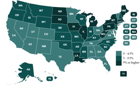
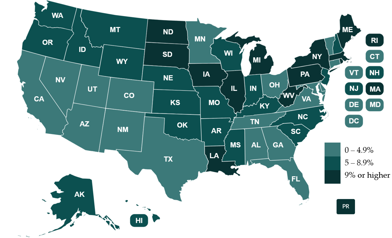
Bridge safety and reliability during service life are influenced by various factors, including traffic loads. Constantly increasing truck weights and the number of overloaded vehicles can lead to excessive deterioration. Currently in the United States, there are more than 623,000 bridges. The percentage of structurally deficient bridges rated as “in poor condition” decreased from 7.5% in 2021 to 6.8% in 2025. It ranges from 1 percent in Texas and Nevada to 19 percent in Iowa. Figure 1 and Table 1 present detailed comparison between various states across the country. Such variation is caused by differences in state policies regarding inspection, maintenance and repair of bridges. Half of the country’s bridges are owned and administered by the states and must be inspected at least once every two years. The other half is owned by counties and cities; however, they often lack sufficient funds for inspection or maintenance. Only very few are privately or federally owned. Over 100 million trips are taken across these structurally deficient bridges every day and the bridge-related system rehabilitation need is estimated at $191 billion [7].

Figure 1. Percentage of structurally deficient bridges, rated as in poor condition [8].

Table 1. Percentage of structurally deficient bridges by the state in 2025 based on Federal Highway Administration (FHWA) National Bridge Inventory (NBI) [9].

US State	Number of Bridges	Percentage of SD Bridges
Iowa	23,716	19.0%
West Virginia	7345	18.0%
South Dakota	5883	16.0%
Maine	2542	15.0%
Rhode Island	787	14.0%
Pennsylvania	23,314	12.0%
Louisiana	12,684	11.0%
North Dakota	4250	11.0%
Michigan	11,397	11.0%
New York	17,666	10.0%
Illinois	26,927	10.0%
Massachusetts	5311	9.0%
Missouri	24,647	9.0%
New Hampshire	2549	8.0%
Oklahoma	22,926	8.0%
Nebraska	15,412	8.0%
Alaska	1660	8.0%
Kentucky	14,590	8.0%
Montana	5235	7.0%
North Carolina	19,343	7.0%
Wyoming	3138	7.0%
Wisconsin	14,498	7.0%
South Carolina	9504	6.0%
Mississippi	16,711	6.0%
New Jersey	6825	6.0%
Hawaii	1180	6.0%
Washington	8520	6.0%
Idaho	4646	5.0%
Arkansas	12,978	5.0%
Indiana	19,542	5.0%
Kansas	24,891	5.0%
Oregon	8329	5.0%
California	25,975	5.0%
Connecticut	4363	5.0%
Ohio	26,713	5.0%
Colorado	8990	5.0%
Minnesota	13,551	5.0%
Maryland	5500	4.0%
Tennessee	20,374	4.0%
New Mexico	4033	4.0%
Vermont	2866	4.0%
Utah	3144	4.0%
Virginia	14,143	3.0%
Alabama	16,181	3.0%
Florida	13,070	3.0%
District of Columbia	261	2.0%
Georgia	15,090	2.0%
Texas	56,951	1.0%
Delaware	874	1.0%
Arizona	8587	1.0%
Nevada	2123	1.0%

Overloaded vehicles have a significant impact on bridge structural health. There is a noticeable growth in volume and weight of truck traffic over the years. Recent traffic measurements in Alabama indicated that on average, about 12% of trucks exceed 80 kips. Depending on location within this state, the percentage of vehicles that surpasses the federal legal loads ranges from 5 to 32% [10]. Structural damage is often caused by extreme vehicle loading or collisions involving oversized and/or overweight trucks. In addition, many bridges do not provide adequate clearance due to increasing size of vehicles. The overweight trucks account for 12% of bridge failures [11].

There are several techniques to measure traffic-induced loading, including static and in-motion technologies. Static methods are inherently localized and selective, monitoring only a limited portion of overall highway network traffic. These measurements can be conducted using portable scales or at Weigh Stations which are situated off main roads. Both techniques enable operators to determine compliance with legal weight restrictions. However, because the locations of these stations are widely known among truck drivers, some operators of overloaded vehicles may attempt to avoid them, thereby introducing potential bias into recorded truck weight data [12]. Weigh-in-Motion (WIM) is the process of measuring vehicle characteristics in motion while passing the WIM station. The most common forms are pavement technologies. Pressure or force sensitive sensors are embedded into pavement and enable continuous recording of vehicles without requiring trucks to stop. Bridge WIM (B-WIM) uses an existing bridge as a weigh scale instead of a pressure-sensitive sensor in the road pavement [13]. Regardless of the technology, WIM data can be effectively utilized for various bridge applications. However, the accuracy of live load assessment depends on quality of traffic databases, as measurements are subjected to various uncertainties [14]. Multiple sources provide various guidance on effective processing of Weigh-in-Motion measurements [15,16,17]. Good quality WIM data provides valuable information that enables to:

• Monitor heavy traffic trends and traffic-induced load spectrum;
• Simulate the maximum expected truck load [18];
• Develop the live load statistical model;
• Develop bridge design and rating procedures;
• Identify site-specific models for unusual loading conditions, and other.

The objective of this paper is to extrapolate bridge live load using truck traffic measurements. In 2023 and 2024, a massive Weigh-in-Motion database was provided by Alabama Department of Transportation (ALDOT) in a raw format on a continuous basis. Collected WIM records were processed and validated using different filtering criteria. Vehicular traffic was run over simple span bridges, and site-specific live load effects were computed using influence line analysis. The maximum moments and shear forces in the WIM live load envelope were divided by the corresponding load effects produced by the governing HL-93 loading. Distributions of bias ratios were extrapolated for 75-year period which is the design life of bridges for the strength limit state in the United States. The extrapolation technique presented in this study is consistent with approach developed by Nowak et al. [5] and used in derivation of bridge design live load model currently used in the United States.

2. Massive Data Collection and Processing

In this study, over 150 million vehicles measured by Weigh-in-Motion sensors in 2023 and 2024 in Alabama, United States were processed and used to calculate live load effects and bias factors after necessary filtering. The data were considered representative based on a comparison of traffic patterns evaluated by Iatsko and Nowak [19] using WIM measurements collected between 2006 and 2014. In addition, it should be noted that the Federal Bridge Formula, which restricts the weight-to-length ratio of vehicles crossing bridges, was established in 1975 and remains unchanged to this day.

Data collected by WIM systems installed across different locations in the state was transmitted via cell modems and stored in ALDOT’s data storage system. Then, the records were subsequently transferred on a continuous basis in encrypted format referred to as “raw” format. Raw data is defined as unprocessed and exempt from prior quality control procedures [20]. Records were decrypted and converted into user-friendly format to facilitate subsequent analysis. Structured Query Language (SQL) databases were established to enable efficient post-processing. Measurements contain 131 characteristics for each vehicle, such as the exact time and date of passage, lane occupied, direction of travel, vehicle speed and classification, vehicle type, length, gross vehicle weight, and configuration including the spacing and weight of all axles or axle groups. Most of this information was needed for initial quality control procedures; however, only axle loads and spacings were necessary to compute live load effects.

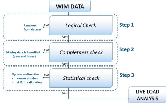
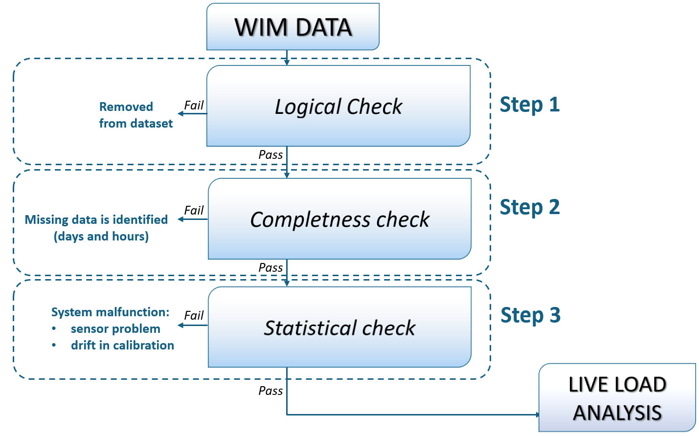
State agencies throughout the United States use various case studies and filtering criteria to verify traffic data quality. However, the Alabama Department of Transportation has not yet established an official state-specific quality control procedure. The filtering algorithm applied in this study for the Alabama WIM data is divided into the following categories (see Figure 2):

Figure 2. Flowchart of a Quality Control procedure.

• Logical check (related to WIM system malfunction or unusual vehicle configuration);
• Completeness check (verifies daily and hourly number of registrations);
• Statistical check (indicates operational problems with sensor, drift in calibration).

Logical checks detect both random errors, which occur occasionally, and systematic errors, which arise more frequently and impact a greater number of records. Obvious errors, including empty rows, duplicated records, invalid station ID, lane number, direction of passage, date, timestamp, null values or single-axle vehicles are also identified. Additionally, logical checks are implemented to exclude vehicles with low gross vehicle weight, as they represent a significant portion of database. A single overloaded truck is estimated to cause road damage equivalent to that caused by 30,000 cars [21]. Lightweight vehicles contribute to the lower tail of the distribution of traffic-induced load effects which is not of importance in bridge live load modeling. Extensive parametric studies were performed by Luszczynska et al. to investigate the influence of filtering criteria selection on the upper tail of load spectra [14]. Excluding this portion of the dataset helps in managing processing constraints and significantly improves the efficiency of computations. Thus, after a discussion with ALDOT, it was proposed to apply the threshold for minimum GVW at 20 kips (89 kN) during the filtering process. Since the load effects are linear-elastic, it can be demonstrated that stress ranges below that value have negligible effect on material fatigue damage using Miner’s Rule. It is also a traditional cutoff used in fatigue studies since light traffic does not contribute significantly to cumulative damage [22]. In addition, trucks with the following configurations were considered unreliable and therefore excluded: (1) less than 5 ft (1.5 m) for steering axle spacing, (2) less than 3.3 ft (1 m) for any other single axle spacing, (3) first axle weight outside of range 6–25 kips (27–111 kN), (4) single axle weight outside of range 1–70 kips (4.5–311 kN), (5) vehicle speed outside of range 10–100 mph (16–160 kph), (6) sum of axle weights ≠ GVW ± 10%, and (7) No. of axles spacing +1 ≠ No. of axle weights.

A completeness check identified missing records in an accumulated dataset and ensured that enough valid records remain for further analysis. Data may be absent due to factors such as system malfunctions or communication failures. An algorithm was implemented to verify data presence for each hour or each day in a month. Missing records were flagged for further investigation of possible causes.

Statistical checks were applied to examine changes in traffic composition, gross vehicle weights, and vehicle configurations. Monthly data was examined to detect irregularities in load patterns. The reasons for anomalies can be communication failures, operational problems with sensors, or calibration drift over time. These checks primarily focus on accumulated data rather than individual records. One of the most common statistical checks on Class 9 vehicles (5-Axle tractor semitrailer) was developed by Minnesota DOT and used in Long-Term Pavement Performance (LTPP) [23]. The statistical checks conducted in this study include an analysis of the percentage of Class 9 vehicles with gross vehicle weight over 100 kips, monthly frequency distributions of GVW, and front axle load spectra by month and by lane.

WIM records that successfully passed logical and completeness check were used for further analysis. Statistical verification identified problems with WIM sites 911 and 964. Quality Control observations were described in detail by Luszczynska et al. [10] and discussed with ALDOT, who scheduled the calibration for these stations. The results from WIM sites 911 and 964 were not considered in the influence line analysis and were excluded from the live load extrapolation described in the following section.

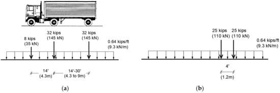
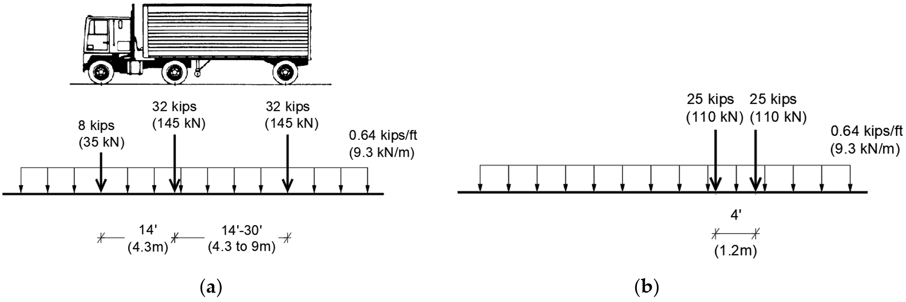
Actual live load effects on bridges were evaluated by computation of maximum moments and shear forces due to the massive WIM database using developed computer programs for influence line analysis. The results were saved separately for each span and location. For each considered span length ranging from 30 ft (9 m) to 200 ft (60 m), the live load effects were also computed for HL-93 design load specified by AASHTO LRFD. “HL” denotes Highway Loading, and “93” refers to the year in which design model was first introduced. To facilitate an interpretation of the results, the maximum moments and shear forces in the WIM live load envelope were divided by the corresponding load effects induced by the governing HL-93 loading (Figure 3). It shall consist of a combination of the:

Figure 3. Vehicular live load model HL-93 according to AASHTO LRFD: (a) Truck and Uniform Load; (b) Tandem and Uniform Load.

• Design Truck or Design Tandem, and
• Design Lane Load.

Each design lane shall be occupied by either the design truck or tandem, coincident with the lane load. The design tandem consists of a pair of 25 kips (110 kN) axles spaced at 4 ft (1.2 m) apart. The transverse spacing of wheels is 6 ft (1.8 m). The design truck is the same as previously adopted HS20-44 with three axles: 8 kips (35 kN), 32 kips (145 kN) and 32 kips (145 kN), spaced at 14 ft (4.3 m) and 14–30 ft (4.3 to 9 m). The design lane load consists of a load of 0.64 klf (9.3 kN/m) which is uniformly distributed in the longitudinal direction [1].

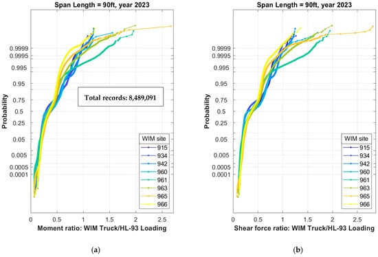
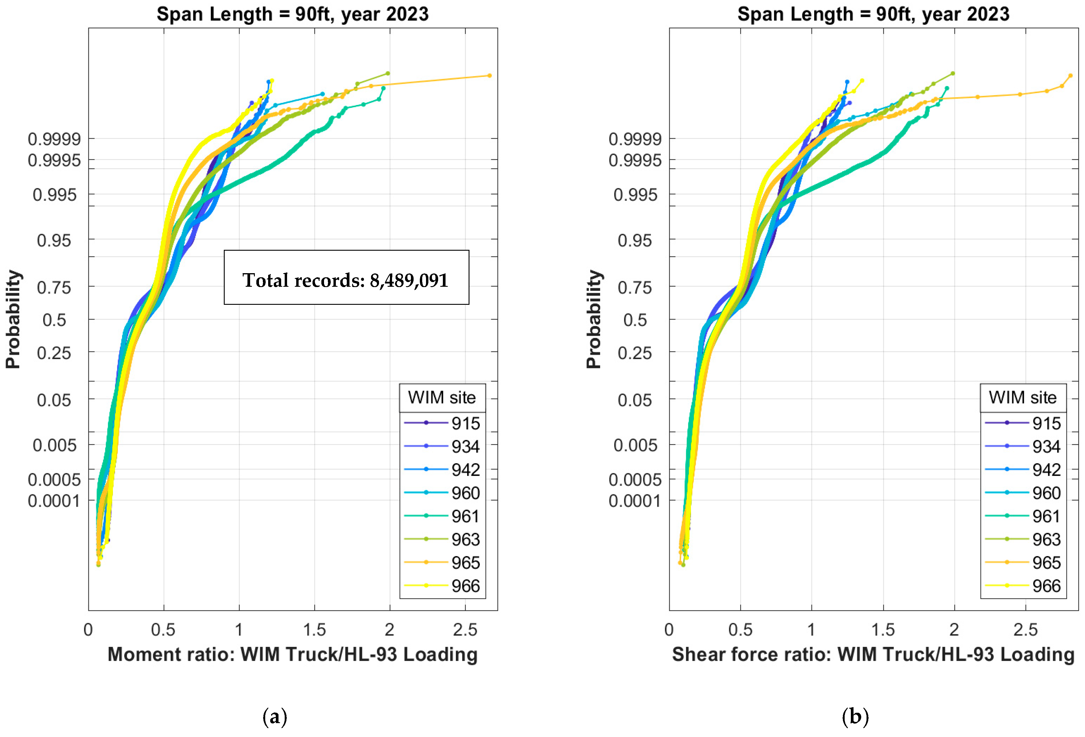
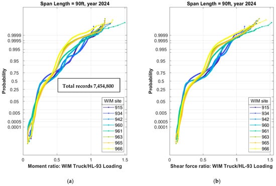
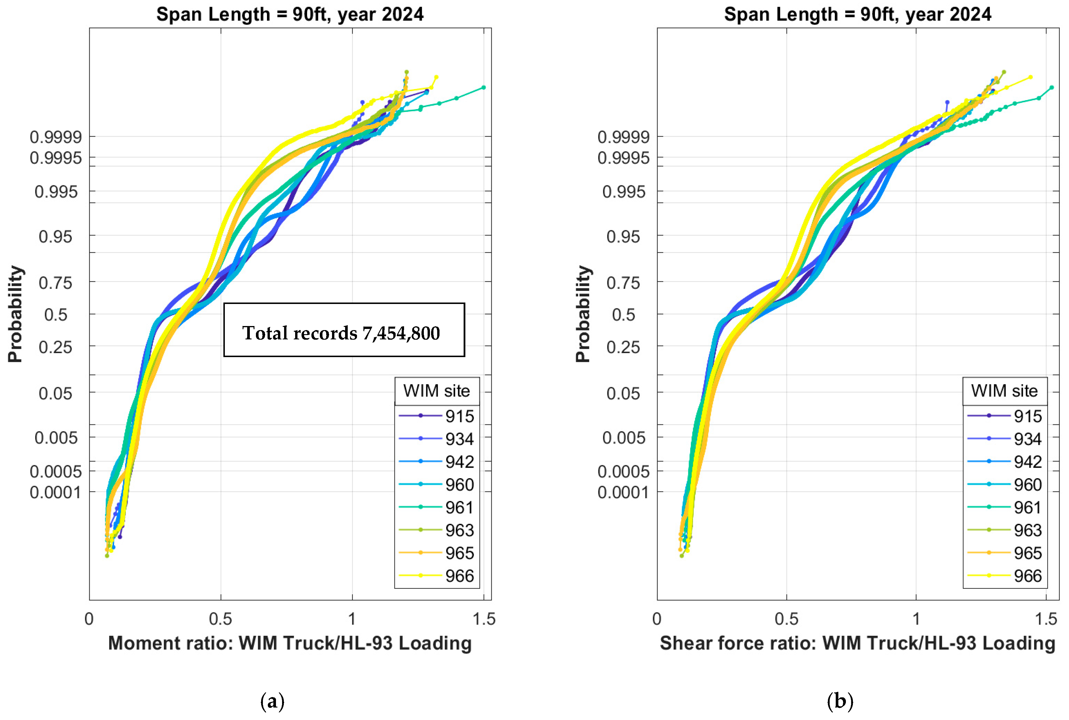
Distribution of live load ratios (WIM Truck/HL-93 Loading) was plotted on a normal probability paper to facilitate interpretation of calculated statistical parameters using available WIM database for each location in the state. Results for selected span equal to 90 ft (27 m) are presented in Figure 4 for data recorded in 2023 and Figure 5 for 2024. A conventional method for presenting statistical data involves utilizing histograms or their corresponding cumulative distribution functions (CDFs). In live load modeling for bridges, particular attention is given to the upper tail of the distribution. For more straightforward graphical interpretation, statistical analysis can be facilitated by plotting the data on normal probability paper. A vertical scale is based on the inverse standard normal variable or corresponding probabilities, while the horizontal scale presents parameter considered in the analysis. It is constructed based on the standard normal non-decreasing CDF (an S-shape function). A probability paper allows for interpretation that would be practically very difficult or even impossible when using a traditional plot. Each value on the vertical axis shows the probability of exceeding a given characteristic on the horizontal axis. The median value corresponds to 0.5 on the vertical axis, while the slope of the function reflects the standard deviation. Additionally, the shape of the CDF can be used to identify the type of distribution. This approach facilitates comparison of critical extreme values within the dataset. Construction and use of the normal probability paper is described in probability textbooks, e.g., Benjamin and Cornell [24] and Nowak and Collins [25]. Computer procedure for Normal Probability Paper is as follows:

Figure 4. CDFs of live load ratio (WIM Truck/HL-93 Loading) for span 90 ft and traffic measured in 2023 in form of: (a) bending moment; (b) shear force.

Figure 5. CDFs of live load ratio (WIM Truck/HL-93 Loading) for span 90 ft and traffic measured in 2024 in form of: (a) bending moment; (b) shear force.

• Arrange the data values {x} in an increasing order. Once ordered, the first (the lowest) value of x will be denoted by x₁, the next value by x₂, etc. up to the last (the largest) value $x_N$;
• Associate with each $x_i$, a cumulative probability $p_i$ equal to:

  $$p_i={\displaystyle \frac{i}{N+1}};$$

  (1)
• For each $p_i$ determine $z_i$:

  $$z_i={\mathrm{\Phi }}^{-1}\left(p_i\right);$$

  (2)
• Plot the coordinates on a standard linear graph paper;
• If the plot appears to follow a straight line, then it is reasonable to conclude that the data can be modeled using normal distribution.

Every data point corresponds to a maximum value of live load effect for each WIM vehicle caused by governing truck position on the span. A probability paper allows for clear representation of massive traffic database with 8,489,091 records (year 2023) plotted in Figure 4 and 7,454,800 measured vehicles (year 2024) in Figure 5. The shape of the CDF curve on normal probability paper indicates the type of distribution. If the CDF is represented by a straight line, the variable may be considered normal. The distributions shown in Figure 4 and Figure 5 demonstrate an irregular shape due to influence of multiple parameters, including varying vehicle types, weights, lengths, and axle spacing within mixed traffic. Vehicles may be fully loaded by weight, empty, partially loaded, or loaded by volume without necessarily being heavy. These scenarios are represented in the distribution’s shape, providing relevant information for bridge experts to assess the patterns of traffic supported by the bridge.

For all analyzed span lengths and WIM sites, the percentage of vehicles with a ratio greater than 1 is very low. The truck load distributions vary depending on the location. The lower tail of load spectra is generally consistent. In the upper tail of distribution, it can be observed that the probability of a WIM load effects to exceed HL-93 model specified by AASHTO LRFD is less than 0.005 (0.5%). Maximum values of a WIM truck to HL-93 load are typically between 1.0–2.0 for most WIM locations and span lengths, except for short span equal to 30 ft for which the highest percentage of vehicles exceeding AASHTO loading is observed. The median value for the moment and shear ratio varies from 0.2 to 0.5 for all considered span lengths. Based on calculated statistical parameters, it can be concluded that truckload spectrum is different depending on WIM site location. Site-specific patterns may be observed especially in the upper tail of CDFs representing the maximum values of load ratio expected at this station.

3. Results of Live Load Extrapolation

3.1. Sorting WIM Database into Strength I and Strength II Limit State

Computed live load effects were further used for load extrapolation. The goal was to predict the maximum values of load ratios for the regular traffic. Therefore, the trucks in WIM database were separated into Strength I and Strength II limit states using sorting strategies performed under NCHRP 12–76 [15] and 12–83 [22]. Strength I that addresses normal service traffic includes legal trucks and vehicles permitted by routine permits. The heaviest vehicles should be included in Strength II load combinations. Typical truck configurations and requirements for state routine permits were analyzed to determine appropriate cut-off limit for separating routine permits from trip permits. Controlled trip permits as well as superloads that occur relatively infrequently were identified and excluded from WIM database using the following criteria:

• Total number of axles is less than three and GVW is more than 50 kips (220 kN);
• Steering axle weight is more than 35 kips (150 kN);
• Individual axle weight is more than 45 kips (200 kN);
• There are seven or more axles;
• GVW exceeds 150 kips (670 kN).

3.2. Maximum Load Effect as a Function of Time Period

The maximum load effect can be considered as a random variable. It is a function of time period which depends on the Average Daily Truck Traffic and distribution (e.g., CDF of WIM moments or shear forces). The mean value of the maximum load effect can be determined for a given CDF, ADTT and period of time, T. The total number of vehicles, N, expected during the considered time period, T (days), is T times ADTT. The expected or mean value of the maximum load effect for specific time T is equal to the live load effect corresponding to probability {1-F [1/N(T)]}, where F(x) is the CDF of WIM live load, which is F⁻¹[1-1/N(T)] where F⁻¹ is the inverse of CDF [24]. For each CDF, the vertical coordinate of the maximum load effect, z_max, is equal to the inverse standard normal distribution function as a function of 1/N:

$$z_{max}={-\mathrm{\Phi }}^{-1}\left({\displaystyle \frac{1}{N}}\right);$$

(3)

For example, if ADTT = 1000 and the considered time period is 1 day, then the vertical coordinate is equal to:

$$z={-\mathrm{\Phi }}^{-1}\left({\displaystyle \frac{1}{1000}}\right)=3.09;$$

(4)

because the number of trucks per day is 1000. Similarly, for the mean maximum 75-year load effect, z, is:

$$z={-\mathrm{\Phi }}^{-1}\left({\displaystyle \frac{1}{\mathrm{27,375,000}}}\right)=5.38;$$

(5)

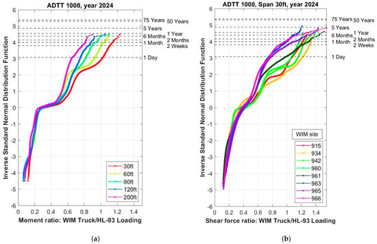
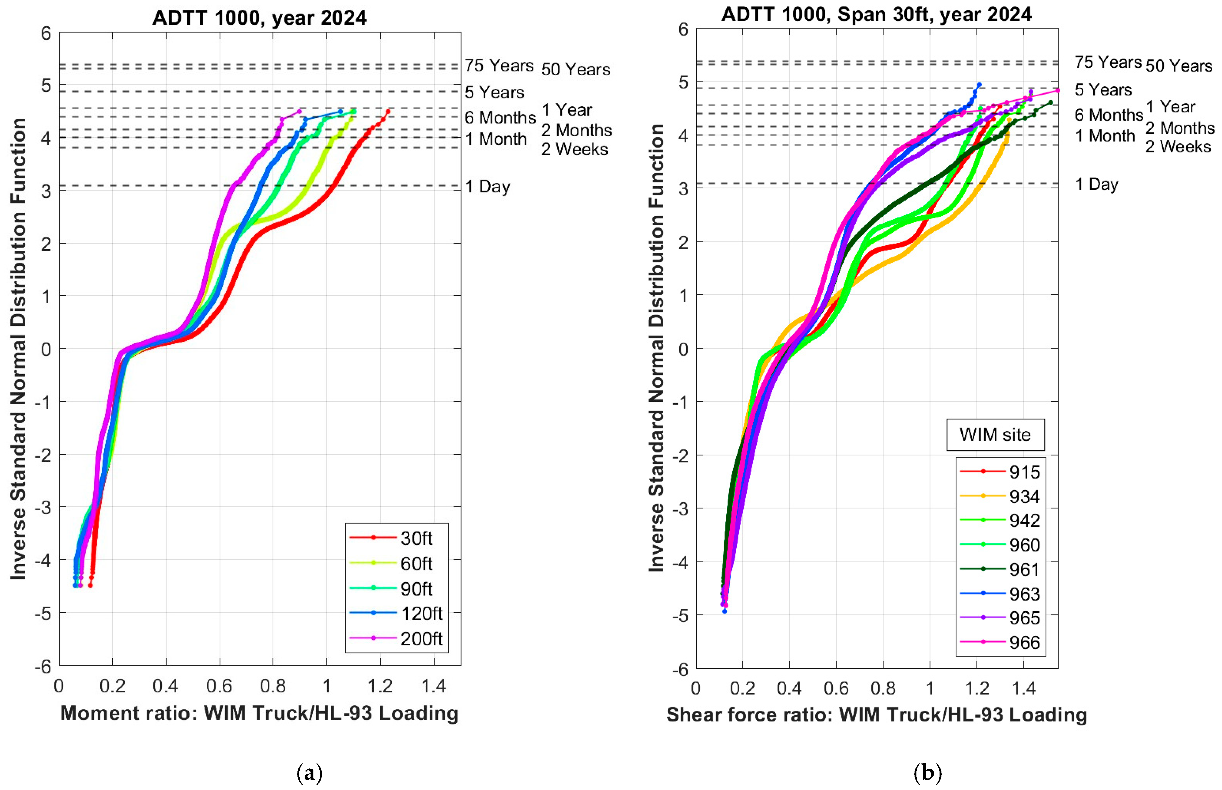
because the number of trucks per 75 years is (1000 trucks) × (365 days) × (75 years) = 27,375,000 trucks. As an example, the cumulative distribution functions of moment and shear force ratios show the vertical coordinates for the ADTT = 1000 and different spans (Figure 6a) as well as different WIM site locations (Figure 6b) presented using the inverse of the standard normal distribution function. Maximum expected values of live load effects depend on the considered time period equal to 75 or 100 years for Strength Limit States and much shorter for Service Limit States. Tabulated values of the CDF for values of the standard normal variate ranging from −4.0 to 4.0 are listed in Table 2 to simplify the understanding of probabilities associated with each WIM station presented in Figure 6. One standard deviation corresponds to the probability of 15% and two standard deviations correspond to the probability of about 2%.

Figure 6. Vertical coordinates for different time periods, ADTT = 1000 and: (a) WIM Site 960 (Whatley) and various span lengths (9, 18, 27, 36 and 60 m); (b) span length 30 ft (9 m) and various WIM sites.

Table 2. Examples of Φ(x) for various values of x.

x	Φ(x)
4.0	0.9999683
3.0	0.99865
2.0	0.9772
1.0	0.841
0.0	0.5
−1.0	0.159
−2.0	0.0228
−3.0	0.00135
−4.0	0.0000317

3.3. Bias Factors for Maximum Expected 75-Year Load Effects

The frequency of trucks on a bridge depends on the traffic volume. After the sorting procedure, the Average Daily Truck Traffic (ADTT) was computed and tabulated in Table 3. Number of days with available data was also summarized. Weigh-in-Motion dataset shared by ALDOT provides lane-specific information for multilane roads, allowing accurate determination of ADTT at each site. The average daily number of truck registrations was determined from total traffic volume and number of operational days individually for each lane.

Table 3. Lane ADTT for regular truck traffic (Strength I Limit State) and vertical coordinates for the 75-year Mean Maximum Moment.

WIM Site	Highway	Number of Days	Total Truck Records, N	Lane ADTT 1	Inverse Standard Normal Variable
915 (Sunflower)	State	589	252,760	429	5.23
918 (Bucksville)	Interstate	121	386,738	3196	5.59
934 (Sumiton)	State	731	104,776	143	5.02
942 (Pine Level)	State	731	933,210	1277	5.43
960 (Whatley)	State	731	295,962	405	5.22
961 (Mobile)	Interstate	568	696,648	1226	5.42
963 (Grand Bay)	Interstate	713	2,281,728	3200	5.59
965 (Shorter)	Interstate	690	2,226,209	3226	5.59
966 (Winfield)	Interstate	731	1,684,255	2304	5.53

¹ WIM data is for multilane cases; lane with maximum ADTT is listed.

Mean maximum live load effects for collected WIM data were computed and compared with the AASHTO model. The bias factors (mean-to-nominal ratios) of live load are equal to ratio of mean maximum 75-year load effect for WIM measurements divided by the corresponding live load induced by the HL-93 design model. These bias factors listed in Table 4 and Table 5 vary as a function of span and average daily truck traffic (ADTT) depending on local conditions. As a result, for each span length, there are 9 values of the maximum 75-year moment and shear corresponding to predicted load ratios for different WIM locations. The variation in the resulting bias factors estimated for each WIM site is primarily driven by site-specific ADTT values and local freight characteristics, with substantially heavier trucks observed particularly in areas near major cities within the state. In addition, the predictions were observed to be highly dependent on the selected upper tail size. This study proves that additional models such as 3S2 [6] or state-specific modified trucks are needed for the bridge rating evaluation. An alternative methodology that utilizes different upper tail sizes for extrapolation was proposed and validated by Lou et al. [26].

Table 4. Bias factors of live load for site-specific ADTT, different spans and WIM sites for 75-year Mean Maximum Moment ¹.

WIM Site			Span Length
	30 ft (9 m)	60 ft (18 m)	90 ft (27 m)	120 ft (36 m)	200 ft (60 m)
915	1.33	1.25	1.20	1.04	0.86
918	1.86	1.67	1.57	1.57	1.76
934	1.43	1.22	1.12	1.12	0.99
942	1.41	1.26	1.17	1.15	1.17
960	1.33	1.25	1.35	1.12	1.66
961	2.94	2.44	2.16	2.10	1.88
963	2.34	2.03	1.89	1.78	1.49
965	2.44	2.19	2.17	2.04	1.79
966	1.48	1.16	1.09	1.16	1.14

¹ Value of inverse standard normal variable depends on ADTT.

Table 5. Bias factors of live load for site-specific ADTT, different spans and WIM sites for 75-year Mean Maximum Shear ¹.

WIM Site			Span Length
	30 ft (9 m)	60 ft (18 m)	90 ft (27 m)	120 ft (36 m)	200 ft (60 m)
915	1.34	1.25	1.27	1.21	1.02
918	1.89	1.65	1.70	1.67	1.48
934	1.47	1.20	1.28	1.29	1.15
942	1.42	1.23	1.22	1.30	1.16
960	1.40	1.24	1.27	1.32	1.18
961	2.86	2.56	2.58	2.51	2.19
963	1.82	1.70	1.76	1.71	1.68
965	2.62	2.43	2.29	2.21	2.12
966	1.71	1.66	1.58	1.60	1.53

¹ Value of inverse standard normal variable depends on ADTT.

Bias factors computed using the extrapolation technique are site-specific. These results may be validated through comparison with independent WIM datasets collected in different states across the United States and Europe. The bias factors for the 75-years maximum moment and shear ratios ranged from 1.98 to 2.77 based on US records and from 2.19 to 2.84 based on European WIM data, demonstrating a significant increase compared with the Ontario data used for the original calibration of the AASHTO LRFD [5]. However, it should be noted that the ADTT and threshold limits used for data selection in the live load analyses differed among these datasets, which influenced the calculated bias factors.

4. Discussion

Extrapolation technique presented in this study was developed by Nowak [5] to determine 75-year extreme live load in original calibration of current AASHTO LRFD Bridge Design Specifications using probabilistic methods. Prior to this research, bridge design in the United States through the 1980’s was based on AASHTO Standard Specifications for Highway Bridges [27] considering the allowable stress and load factor methods. However, the live load model HL-93 was developed based on the available truck including 9250 heavy vehicles measured in 1975 by the Ontario Ministry of Transportation. At that time, the truck population in Ontario was representative of the U.S. trucks. A considerable degree of uncertainty was caused by unpredictability of the future vehicle configurations including axle loads and spacings. The maximum load effect corresponding to 75-year life time was calculated by extrapolation of the available truck survey data. The moments and shears were computed in terms of the proposed HL-93 live load model for the LRFD bridge design code. The mean-to-nominal ratio (bias factor) of live load was defined as the ratio of the maximum 75-year load effect and the design value. The calculated mean maximum moments divided by corresponding HL-93 moments (ADTT = 1000) for simple spans equal to 30, 60, 90, 120 and 200 ft (9, 18, 27, 36 and 60 m) were accordingly 1.35, 1.32, 1.31, 1.29 and 1.23. The calculated mean maximum shears divided by corresponding HL-93 shears (ADTT = 1000) for simple spans equal to 30, 60, 90, 120 and 200 ft (9, 18, 27, 36 and 60 m) were accordingly 1.25, 1.23, 1.28, 1.22 and 1.17. The bias factors vary as a function of span; however, it was observed that the variation is reduced for the proposed new LRFD live load (HL-93) in comparison to previously used HS20 loading. Current Alabama-specific research shows that the variation of bias factors is significantly higher and therefore the revision of current AASHTO load model may be beneficial. Similar line girder programs can be developed and successfully used for continuous and multi-span bridges, as well as for the analysis of multilane loading scenarios in the transverse direction. For more complex structures, the finite element method may be advantageous [28].

In addition, live load factor should be considered together with the HL-93 design model and according to the AASHTO LRFD Bridge Design Specifications should be taken as 1.75 for Strength I. Extrapolation of Alabama-specific loads presented in this research showed that this value is exceeded only by trucks recorded at interstate highways, whereas the bias factor remained lower for all state highways. It should be noted that the WIM measurements used for this analysis were collected using sensors embedded in the roadway. Consequently, a portion of the recorded vehicles may not have possessed permits authorizing them to cross the bridge. It is also necessary to consider whether such a substantial increase of bias ratios is realistic and physically achievable. Trucks have inherent structural limits that determine the maximum load that can be carried by each axle. While axle capacities and loading capabilities have increased over time due to advances in technology, these vehicles are still constrained by fundamental physical and structural limitations.

Most of the statistics were presented in form of the cumulative distribution functions (CDFs) plotted on the normal probability paper. CDFs are used to compare the critical extreme values within datasets. This approach is particularly significant in bridge engineering, where the upper tail of the load spectrum is of concern. The assessment of traffic-induced load effects on any bridge can be effectively conducted using millions of vehicles collected at Weigh-In-Motion stations located in different geographic regions across the United States and many other countries. For future research and further reliability analysis, it is recommended to assume that the mean maximum live load is equal to the mean for all WIM locations plus 1.5 standard deviations for which the probability of exceeding is about 5%. Additionally, coefficients of variation (COV) defined as the ratios of standard deviation to mean should be computed.

5. Conclusions

The bias factors of live load for Strength Limit State are developed using available WIM data. This database includes over 150 million records covering two-year measurements for each location. Filtering procedures are developed to exclude lightweight vehicles and questionable measurements. The cumulative distribution functions are plotted on normal probability paper for calculated live load effects. The WIM truck moments and shears are computed for a wide range of spans from 30 to 200 ft (9 to 60 m). The CDF’s show that truck traffic is site-specific, however state-specific patterns may be observed.

Legal trucks and vehicles permitted by routine permits were sorted out and used to extrapolate load effects. The mean maximum 75-year moments and shears for selected spans were divided by corresponding HL-93 live load. Resulting bias ratios are the function of time period. Therefore, ADTT was evaluated individually at each WIM site location. The statistical parameters for the static component of live load effect for simple span bridges indicate that the maximum 75-year bias ratios (λ_75years) vary from:

• 1.09 to 2.94 for moment at interstate highways;
• 0.86 to 1.66 for moment at state highways;
• 1.48 to 2.86 for shear at interstate highways;
• 1.02 to 1.47 for shear at state highways.

Although the available WIM databases are site-specific, they can be considered representative of the state of Alabama. Bias factors for WIM stations on interstate highways exceed 1.75, indicating the need to review the AASHTO bridge design provisions, including the HL-93 model and the calibrated live load factor for Strength I Limit State. To assess the impact of heavy trucks on bridge structures, the internal forces can be calculated for wide range of vehicle configurations, number of axles, axle weights and spacings using influence line analysis. Derived statistical parameters may be used for accurate development of state-specific live load statistics. The research allows to determine the actual loading conditions which serve as the basis for prediction of structural safety and continuous monitoring at regular intervals of overweight vehicles that mostly impact bridge structures. Constantly increasing truck weights can lead to excessive deterioration. Therefore, the results confirm the importance of traffic data collection and use of reliability-based analysis. However, the authors think that bias factors close to 3.0 are conservative. If an extremely heavy truck is present in one traffic lane, the adjacent lane will most likely be occupied by a vehicle with an average weight. Consequently, each girder will be subjected to only a fraction of the load effects generated by vehicles occupying adjacent lanes.

In addition, the frequency of overload events is a critical factor in bridge performance assessment. Even if a superload vehicle produces exceptionally large load effects, its significance is limited if such an event occurs only once during the service life of the bridge, representing an extreme outlier in the cumulative distribution function. In practice, the percentage of vehicles producing load effects that exceed a factor of 1.0 is small. To further refine the extrapolation method, it is recommended to perform fatigue analysis and predict the remaining lifetime by estimating the number of load cycles.

References

- LRFDBDS-9; AASHTO LRFD Bridge Design Specifications, 9th ed. American Association of State Highway and Transportation Officials: Washington, DC, USA, 2020.
- Agarwal, A.C.; Wolkowicz, M. Ontario Commercial Vehicle Survey; Interim Report; Research and Development Branch, Ontario Ministry of Transportation and Communications: Downsview, ON, Canada, 1976. [Google Scholar]
- Nowak, A.S.; Hong, Y.K. Bridge Live-Load Models. J. Struct. Eng. 1991, 117, 2757–2767. [Google Scholar] [CrossRef] [Scilit]
- Nowak, A.S. NCHRP Report 368: Calibration of LRFD Bridge Design Code; Transportation Research Board: Washington, DC, USA, 1999. [Google Scholar]
- Ramesh Babu, A.; Iatsko, O.; Nowak, A.S. Comparison of Bridge Live Loads in the US and Europe. Struct. Eng. Int. 2019, 29, 84–93. [Google Scholar] [CrossRef] [Scilit]
- AASHTO MBE-3; AASHTO Manual for Bridge Evaluation, 3rd ed. American Association of State Highway and Transportation Officials: Washington, DC, USA, 2018.
- American Society of Civil Engineers. Report Card for America’s Infrastructure 2025. Available online: www.infrastructurereportcard.org (accessed on 23 November 2025).
- American Road & Transportation Builders Association. Bridge Report 2025. Available online: https://www.artbabridgereport.org/state/map (accessed on 8 June 2026).
- Federal Highway Administration. Bridge Condition by Highway System 2024. FHWA, U.S. Department of Transportation. Available online: https://www.fhwa.dot.gov/Bridge/nbi/no10/condition24.cfm (accessed on 8 June 2026).
- Luszczynska, A.K.; Roszczenko, R.; Nowak, A.S. Fusion of WIM and Permit Data to Monitor Alabama Traffic; Final Report submitted to Alabama Department of Transportation; Auburn University: Auburn, AL, USA, 2025. [Google Scholar]
- Nowak, A.S.; Iatsko, O. Are Our Bridges Safe? National Research Council: The Bridge; The National Academies Press: Washington, DC, USA, 2018; Volume 48, pp. 26–30. [Google Scholar]
- Stawska, S. Impact of Overloaded Vehicles on Bridges. Doctoral Dissertation, Auburn University, Auburn, AL, USA, 2021. [Google Scholar]
- International Society for Weigh-in-Motion. WIM Data for Bridge Engineering: What Should I Know What Should I Do? ISWIM: Dübendorf, Switzerland, 2022. [Google Scholar]
- Luszczynska, A.K.; LaMondia, J.J.; Nowak, A.S. Quality Evaluation of Weigh-in-Motion Traffic Data for Bridge Live Load Modeling. In Proceedings of the 2026 TRB Annual Meeting, Washington, DC, USA, 11–15 January 2026. [Google Scholar]
- Sivakumar, B.; Ghosn, M.; Moses, F. NCHRP Report 683: Protocols for Collecting and Using Traffic Data in Bridge Design; Transportation Research Board: Washington, DC, USA, 2008. [Google Scholar]
- O’Brien, E.; Enright, B. Modeling Same-Direction Two-Lane Traffic for Bridge Loading. Struct. Saf. 2011, 33, 296–304. [Google Scholar] [CrossRef] [Scilit]
- Portela, E.L.; Lou, P.; Bittencourt, T.N.; Nassif, H.H. Reliability assessment of prestressed bridges in Brazil using WIM data. In Bridge Maintenance, Safety, Management, Life-Cycle Sustainability and Innovations, 1st ed.; Taylor & Francis Group: London, UK, 2021; pp. 1347–1354. [Google Scholar] [CrossRef] [Scilit]
- Nowak, A.S.; Lutomirska, M. The development of live load for long span bridges. Bridge Struct. 2010, 6, 73–79. [Google Scholar] [CrossRef] [Scilit]
- Iatsko, O.; Nowak, A.S. WIM-Based Live Load for Alabama Bridges; Final Report Submitted to Alabama Department of Transportation; Auburn University: Auburn, AL, USA, 2017. [Google Scholar]
- Pelphrey, J.; Higgins, C.; Sivakumar, B.; Groff, R.L.; Hartman, B.H.; Charbonneau, J.P.; Rooper, J.W.; Johnson, B.V. State-Specific LRFR Live Load Factors Using Weigh-in-Motion Data. J. Bridge Eng. 2008, 13, 339–350. [Google Scholar] [CrossRef] [Scilit]
- van Loo, H.; Žnidarič, A. Guide for Users of Weigh-in-Motion: An Introduction to Weigh-in-Motion; ISWIM, International Society for Weigh-in-Motion: Dübendorf, Switzerland, 2021. [Google Scholar]
- Wassef, W.W.; Kulicki, J.M.; Nassif, H.; Mertz, D.; Nowak, A.S. NCHRP Project 12-83: Calibration of AASHTO LRFD Concrete Bridge Design Specifications for Serviceability; Transportation Research Board: Washington, DC, USA, 2014. [Google Scholar]
- Hellenbeck, M. WIM Data Quality Assurance. In Proceedings of the National Traffic Data Acquisition Conference, Rocky Hill, CT, USA, 18–22 September 1994. [Google Scholar]
- Benjamin, J.R.; Cornell, C.A. Probability, Statistics, and Decisions for Civil Engineers; McGraw-Hill: New York, NY, USA, 1970. [Google Scholar]
- Nowak, A.S.; Collins, K.R. Reliability of Structures, 2nd ed.; CRC Press: Boca Raton, FL, USA, 2013. [Google Scholar]
- Lou, P.; Yang, C.; Nassif, H. Prediction of Maximum Live-Load Effects for Bridges Based on Weigh-in-Motion Data. Transp. Res. Rec. 2025, 2679, 1034–1051. [Google Scholar] [CrossRef] [Scilit]
- AASHTO HB-17; AASHTO Standard Specifications for Highway Bridges. American Association of State Highway and Transportation Officials: Washington, DC, USA, 2002.
- Luszczynska, A.K.; Roszczenko, R.; Nowak, A.S. Permit-Based Live Load Model for Complex Truss Bridges. In Proceedings of the 12th New York City Bridge Conference, New York, NY, USA, 25–26 August 2025. [Google Scholar]
Disclaimer/Publisher’s Note: The statements, opinions and data contained in all publications are solely those of the individual author(s) and contributor(s) and not of MDPI and/or the editor(s). MDPI and/or the editor(s) disclaim responsibility for any injury to people or property resulting from any ideas, methods, instructions or products referred to in the content. |
© 2026 by the authors. Licensee MDPI, Basel, Switzerland. This article is an open access article distributed under the terms and conditions of the Creative Commons Attribution (CC BY) license.