


Abstract
Asphalt bridge deck pavements are highly susceptible to rutting, shoving, and interlayer slippage under high-temperature traffic conditions, where interlayer shear stress plays a decisive role. To clarify the coupled effects of thermal gradients and moving loads, this study developed a sequential three-dimensional thermo-mechanical finite element model for a double-layer pavement in Zhongshan, China. Field-recorded air temperature, solar radiation, sunshine duration, and wind speed were used to define transient thermal boundaries. The calculated temperature field was then transferred to a fully bonded moving-load model with dual rectangular contact areas and braking-induced longitudinal traction. Axle load, roadway slope, braking coefficient, and the thicknesses of the SMA-13 and AC-20 layers were varied. The predicted temperature fluctuation attenuated and the peak time was delayed with depth. The pavement surface reached 58.95 °C at 13:00, whereas the bottom of the asphalt overlay reached 46.99 °C at 17:00. Under the adopted 14:00 near-peak summer condition, increasing axle load amplified the overall response and raised the maximum asphalt-layer shear response from 0.172 to 0.223 Mpa. Roadway slope mainly affected traffic-direction stress transfer. Increasing the braking coefficient from 0 to 0.7 increased longitudinal shear response from 57.9 to 161.2 kPa in the asphalt layers and from 56.4 to 112.6 kPa near the AC-20/concrete interface. Increasing SMA-13 thickness reduced thermal and mechanical demand in the underlying layers, whereas increasing AC-20 thickness reduced the response near the concrete deck but shifted part of the tensile and shear demand toward the upper asphalt layer.
1. Introduction
Asphalt pavement on a cement concrete bridge deck is a relatively thin multilayer system subjected simultaneously to environmental temperature variation, moving traffic loads, and restraint from the underlying deck slab. In addition to providing the required surface functions, the asphalt overlay must accommodate the pronounced differences in stiffness, thermal expansion, and deformation characteristics between asphalt mixtures and cement concrete. Previous reviews have identified temperature sensitivity, structural compatibility, and interlayer performance as persistent concerns in this type of bridge deck pavement [1]. The problem becomes more pronounced at elevated temperatures, when the stiffness of the asphalt courses decreases and the pavement becomes more susceptible to rutting, shoving, fatigue cracking, and interlayer-related distress. On curved or sloped bridge sections, tire–bridge interaction, geometric effects, and longitudinal traffic actions further modify the stress state of the pavement [2,3].
The transfer of traffic and thermal actions through the multilayer system depends strongly on the interlayer condition. Finite element analyses and full-scale tests have shown that bonding quality affects stress transfer and deformation compatibility between adjacent pavement layers [4]. More recent investigations have evaluated bridge deck pavement shear behavior through combined experimental and numerical analysis [5], inclination shear testing of concrete deck–asphalt overlay systems [6], inclined shear fatigue testing of asphalt overlays on Portland cement concrete [7], and mechanical and experimental assessment of waterproof adhesive layers on concrete bridge decks [8]. Bond performance between cement concrete substrates and asphalt ultra-thin overlays has also been examined under different conditioning and loading conditions [9]. Recent studies have advanced waterproof and bonding-layer design through modified bonding materials, strength-based laboratory evaluation, surface-treatment optimization, and combined numerical–experimental assessment of interlayer resistance [8,10,11,12]. However, experimentally measured bond strength and the stresses obtained from a structural model represent different quantities. Under the fully bonded assumption adopted in this study, the calculated stresses describe the interface-adjacent shear demand transferred through an intact multilayer system, rather than interface strength, slip, or debonding.
Temperature affects the pavement response through both the nonuniform thermal field and the temperature dependence of asphalt-mixture properties. Solar radiation, ambient air temperature, wind, convection, and long-wave radiation cause the temperature fluctuation to attenuate with depth and delay the occurrence of internal temperature peaks [13]. Recent thermo-mechanical studies have incorporated detailed environmental conditions and tire–bridge interaction into curved-ramp bridge deck pavement analyses [14], while three-dimensional multiscale methods have been used to connect structural response with local material damage [15]. More recent investigations have further incorporated measured environmental conditions, viscoelastic asphalt behavior, interlayer contact, moving traffic loads, and layer-thickness variations into the dynamic analysis of asphalt pavements on concrete bridge decks [16].
Related investigations on steel–concrete composite and steel bridge decks have also demonstrated that temperature and traffic loading should not be considered independently. Temperature–load coupling has been shown to alter the stress, deformation, and permanent-deformation characteristics of multilayer bridge deck pavements [17,18,19,20]. Dynamic analyses of asphalt pavements on concrete bridge decks have further considered vehicle load, speed, interlayer contact, and structural thickness under temperature-dependent conditions [16]. For steel bridge deck systems, recent studies have incorporated realistic thermal fields and nonuniform loading into thermo-mechanical simulations [21,22], while multiscale finite element frameworks have linked global bridge deformation to local pavement stress concentrations and structural-configuration effects [23]. Recent analytical studies have also examined the dynamic response of steel bridge deck pavement systems [24], while waterproof-system configuration and double-layer heterogeneous arrangements have been shown to affect stress transfer and interlayer response [25,26].
Recent studies have expanded this work to local interfaces and special pavement systems. Coupled temperature–dynamic loading has been considered in the analysis of repaired interfaces on steel bridge decks [27], and the response of hot-mixed epoxy asphalt concrete pavement has been evaluated under combined thermal and traffic actions [28]. Experimental studies have also examined interlayer shear behavior in specialized bridge deck pavement systems [29], while temperature–humidity coupling has been shown to affect steel–asphalt interface behavior [30]. Related pavement research has further demonstrated that mixture performance may depend on the characteristics of the supporting structure [31].
Despite this progress, several issues remain insufficiently clarified for double-layer asphalt pavements on cement concrete bridge decks. First, many mechanical analyses rely on uniform temperatures, prescribed gradients, or isolated thermal states, whereas the sequential transfer of a transient temperature field derived from monitored environmental conditions into a moving-load model has received comparatively less attention, particularly in hot-humid regions. Such depth-dependent temperature variation is important because the upper and lower asphalt courses may reach their peak temperatures at different times and therefore exhibit different stiffness levels during the same loading event. Second, axle load, roadway slope, and horizontal traffic action are often examined using different structures, thermal conditions, and response indices, making their respective effects on longitudinal and transverse interface-adjacent shear responses difficult to compare directly. In particular, braking-induced traction acts in the traffic direction and must be transferred through the asphalt overlay, yet its effect has not been consistently evaluated together with vertical axle load and roadway slope under the same modeling framework. Third, changes in upper- and lower-layer thicknesses affect not only the total overlay thickness but also the heat-transfer path, temperature distribution, relative stiffness, and mechanical load transfer. Their distinct roles in thermal attenuation and response redistribution therefore require separate examination.
To address these questions, this study develops a field-informed representative numerical case for a double-layer asphalt pavement on a cement concrete bridge deck in Zhongshan, Guangdong Province. Hourly ambient air temperature, total solar radiation, effective sunshine duration, and daily mean wind speed were used to define the transient environmental boundary conditions. These meteorological records served as model inputs and did not constitute direct measurements of pavement-surface temperature, internal temperature, stress, or strain. A transient heat-transfer model was first established to determine the depth- and time-dependent temperature distribution. The resulting nonuniform temperature field was then transferred sequentially to a three-dimensional mechanical model. Moving dual-rectangular contact loads and braking-induced longitudinal traction were applied to an intact, fully bonded pavement system.
The specific objectives were to: (1) characterize the attenuation and time lag of pavement temperature through the structural depth under representative summer and winter conditions; (2) quantify the peak longitudinal and transverse interface-adjacent responses under moving vertical and braking loads; and (3) compare the effects of axle load, roadway slope, braking coefficient, and upper- and lower-asphalt-layer thicknesses within the investigated ranges. By evaluating these factors under the same thermal state, material representation, interface condition, and loading framework, the study distinguishes their respective effects on longitudinal shear transfer and thickness-dependent response redistribution.
2. Development of the Sequential Thermo-Mechanical Finite Element Framework
2.1. Engineering Background, Representative Structure, and Research Framework
The field-informed numerical case was established using meteorological records collected in Zhongshan, Guangdong Province, a hot-humid subtropical region in southern China. The available environmental records included hourly ambient air temperature, total daily solar radiation, effective sunshine duration, and daily mean wind speed. A representative summer day was selected to characterize an unfavorable high-temperature condition, while a representative winter day was used to examine seasonal differences. These monitored meteorological records were used to define the environmental thermal boundary conditions rather than as direct measurements of the internal pavement response.
The bridge deck pavement considered in this study consists of a 4 cm SMA-13 surface course, a 6 cm AC-20 lower course, and a 10 cm C30 concrete deck slab. This configuration represents a typical asphalt overlay system used on concrete bridge decks in hot-humid regions of southern China. It was selected to capture the pronounced differences in thermal and mechanical properties between the asphalt overlay and the concrete substrate, which are important for the transfer of interlayer stress. The model was intended to represent a typical bridge deck pavement configuration rather than to reproduce all structural details of a specific bridge.
The numerical investigation was conducted using a sequential thermo-mechanical procedure. First, field-informed meteorological conditions were used to establish the transient temperature field of the bridge deck pavement. Second, the calculated temperature field was transferred to the mechanical model as a predefined field. Moving dual-rectangular wheel loads, consisting of vertical contact pressure and braking-induced longitudinal traction, were then applied. Finally, the effects of axle load, roadway slope, braking coefficient, and upper- and lower-layer thicknesses on the mechanical response were evaluated.
2.2. Governing Equations and Environmental Thermal Boundary Conditions
The transient temperature field of the bridge deck pavement is governed by heat conduction within the multilayer system. For an isotropic material, the temperature is expressed as a function of spatial coordinates and time, and the heat flux follows Fourier’s law. The corresponding thermal diffusivity is determined by the thermal conductivity, specific heat capacity, and density of the material, as expressed in Equations (1)–(3).
Since the bridge deck pavement is directly exposed to the atmospheric environment, it is subjected to combined effects of solar radiation and convective heat exchange. As a result, the air temperature exhibits a periodic variation, and its influence on the pavement temperature field can also be reasonably approximated as a periodic function in the finite element analysis.
- (1)
- Solar radiation
Based on previous research findings [13], the effect of solar radiation can be approximated using the following function according to its daily variation pattern, as expressed in Equation (4).
where q0 is the maximum solar radiation at noon, q0 = 0.131 mQ, Q is the total daily solar radiation (J/m2), c is the actual effective sunshine duration (h), and ω is the angular frequency, defined as ω = 2π/24 (rad).
The discontinuous solar-radiation function was expanded into a cosine Fourier series to obtain a smooth time-dependent heat-flux input for the finite element analysis. Based on the adopted formulation, a series order of (k = 30) was used to provide sufficient numerical accuracy for the present analysis. The resulting Fourier-series representation is given in Equations (5) and (6).
where a0 = 2q0/mπ.
- (2)
- Air temperature and convective heat exchange
Because the daytime heating and nighttime cooling processes are asymmetric, a single sinusoidal function cannot accurately reproduce the 24 h air-temperature variation. Therefore, a combined sinusoidal function was adopted to describe the daily temperature cycle, as expressed in Equation (7).
where is the daily mean air temperature (°C), , is the daily temperature amplitude (°C), , and are the daily maximum and minimum temperatures, respectively, ω is the angular frequency (rad), ω = 2π/24, and t0 is the initial phase, defined as the time difference between the peak solar radiation and the peak air temperature plus 7 h. In the calculation, t0 can be taken as 9 accordingly, and the starting time is set at midnight (0:00).
The convective heat-transfer coefficient between the pavement surface and the atmosphere was determined from the daily mean wind speed using Equation (8).
where hc is the convective heat transfer coefficient (W/(m2·°C)), and vω is the daily mean wind speed (m/s).
- (3)
- Long-wave radiation exchange
The thermal boundary condition for effective ground radiation was applied using Equation (9).
where qF is the effective ground radiation (W/(m2·°C)), ε is the pavement emissivity, taken as 0.81 for asphalt pavements, σ is the Stefan–Boltzmann constant, , is the pavement surface temperature (°C), Ta is the air temperature (°C), and Tz is the absolute zero temperature (°C), Tz = −273 °C.
The environmental thermal inputs were obtained from meteorological observations collected in Zhongshan, Guangdong Province, which has a hot-humid subtropical climate. A representative summer day was selected to characterize the unfavorable high-temperature condition, while a representative winter day was used to examine seasonal differences. The field-monitored environmental inputs included hourly ambient air temperature, total daily solar radiation, effective sunshine duration, and daily mean wind speed. These records were used exclusively to define the time-dependent environmental boundary conditions of the thermal model.
For the representative summer day, the total solar radiation, effective sunshine duration, and daily mean wind speed were 24.5 MJ/m2, 6.81 h, and 2.4 m/s, respectively. The corresponding winter values were 16.9 MJ/m2, 4.71 h, and 3.4 m/s. The hourly air-temperature records used in the thermal analysis are listed in Table 1.
Table 1.
Hourly ambient air temperatures used as thermal boundary inputs for the representative summer and winter days in Zhongshan.
These environmental inputs were subsequently implemented as time-dependent surface boundary conditions in the transient thermal finite element model described in Section 2.3.
2.3. Transient Thermal Finite Element Model
2.3.1. Model Development
To investigate the transient thermal response of the bridge deck pavement, a three-dimensional finite element temperature field model was developed in ABAQUS. The bridge deck pavement structure consisted of a 4 cm SMA-13 surface course, a 6 cm AC-20 lower course, and a 10 cm C30 cement concrete deck slab, as shown in Figure 1. The modeled bridge deck had dimensions of 6 m × 6 m × 0.2 m. The positive X-direction corresponds to the traffic direction, the Y-direction is perpendicular to the traffic direction, and the Z-direction represents the depth direction.
Figure 1.
Type and Thickness of Structural Layers.
The in-plane dimensions were selected to be substantially larger than the wheel-load contact area to reduce the influence of the model boundaries on the local response. The loading region was locally refined so that the thermal and mechanical models could use a consistent discretization in the area of interest. The transient heat-transfer analysis employed DC3D8R eight-node linear heat-transfer brick elements. The finite element mesh is shown in Figure 2, and the thermal properties used in the analysis are summarized in Table 2.
Figure 2.
Temperature Field Model.
Table 2.
Thermal parameters used in the transient heat-transfer analysis.
2.3.2. Model Assumptions and Implementation
To simplify the analysis, the following assumptions were adopted in the transient thermal analysis:
- (1)
- Each structural layer was treated as homogeneous and isotropic.
- (2)
- Temperature and heat flux were assumed to be continuous across adjacent layers.
- (3)
- Because the atmospheric and radiative boundary conditions were applied approximately uniformly over the pavement surface, heat transfer was assumed to be dominated by the depth direction, and in-plane temperature gradients were neglected.
- (4)
- Except for the parameters explicitly defined as temperature-dependent, the remaining thermal properties were treated as constants.
These assumptions are appropriate for characterizing the overall depth-dependent thermal response of the multilayer pavement system under approximately uniform environmental exposure. However, the model does not account for localized thermal heterogeneity caused by shading, nonuniform surface conditions, water accumulation, spatial variability in material properties, or interlayer thermal contact resistance. Therefore, the predicted temperature field should be interpreted as a representative system-level response rather than a description of localized thermal anomalies.
The thermal boundary conditions were implemented through user-defined subroutines in ABAQUS. The FILM subroutine was employed to simulate convective heat exchange between the pavement surface and the atmosphere, while the DFLUX subroutine was used to apply the time-dependent solar radiation flux and effective long-wave radiation flux. Through these treatments, the model was able to capture the transient temperature evolution within each pavement layer under field-informed environmental conditions and to provide the temperature input required for the subsequent thermo-mechanical coupling analysis.
The transfer of the calculated temperature field and the establishment of the corresponding mechanical model are described in Section 2.4.
2.3.3. Initial and Boundary Conditions and Thermal Cycling
For the representative summer and winter cases, the initial temperatures of the entire pavement system were uniformly set to 31.6 and 9.2 °C, respectively, corresponding to the daily mean ambient air temperatures of the selected meteorological days. The upper surface was subjected to the time-dependent solar radiation, convective heat transfer, and long-wave-radiation boundary conditions described in Section 2.2. The four lateral surfaces and the bottom surface of the concrete deck slab were treated as thermally insulated.
To minimize the influence of the assumed initial temperature, the environmental thermal boundary conditions were applied continuously for three consecutive 24 h cycles. Periodic thermal stability was considered to have been achieved when the maximum absolute temperature difference at corresponding times between two consecutive cycles was less than 0.1 °C. The temperature field obtained during the third cycle was subsequently used for the temperature-field analysis and sequential thermo-mechanical calculation.
2.4. Sequential Temperature-Field Transfer and Mechanical Model
2.4.1. Temperature-Field Transfer and Mechanical Boundary Conditions
Following the transient heat-transfer analysis, the calculated temperature field was introduced into the mechanical model as a predefined field. The stress-free reference temperature used for calculating thermal strain was set to 31.6 °C. The thermal and mechanical models adopted the same geometric configuration, allowing the temperature distribution to be assigned consistently to the corresponding structural layers. The analysis was sequentially coupled: the calculated temperature field affected the temperature-dependent material properties and thermal deformation in the mechanical analysis, whereas the mechanical response was assumed not to influence the preceding heat-transfer process.
The mechanical analysis employed C3D8R eight-node linear brick elements with reduced integration. The four lateral surfaces were constrained in their respective normal directions, while vertical deformation of the lateral surfaces was permitted. The bottom surface of the concrete deck slab was fully fixed. These boundary conditions were adopted to prevent rigid-body motion and provide a simplified representation of the structural restraint of the bridge deck pavement system.
The temperature field at 14:00 on the representative summer day was transferred to the mechanical model as a fixed high-temperature condition for the subsequent parametric analyses. At this time, the ambient air temperature reached its daily maximum, the pavement-surface temperature remained close to its peak at 13:00, and the lower asphalt layer continued to warm toward its later peak at 17:00. The 14:00 field was therefore selected to represent a nonuniform near-peak thermal state of the asphalt overlay. This selection was intended to provide a consistent thermal background for comparing the effects of axle load, roadway slope, braking coefficient, and pavement thickness, rather than to identify the time of maximum interlayer shear response over the full daily cycle.
2.4.2. Interface Treatment
The interface between the SMA-13 surface course and the AC-20 lower course, as well as the interface between the AC-20 layer and the concrete deck slab, was modeled using tie constraints. Accordingly, displacement continuity was imposed across each interface, and relative slip or separation was not permitted during the mechanical analysis. Previous studies have shown that the contact state and bonding quality at asphalt–concrete and asphalt–asphalt interfaces can alter stress transfer and the overall structural response of multilayer pavements [16,32]. The tie formulation adopted here therefore represents a reference condition with continuous load transfer rather than the full range of interface states that may develop during service.
This treatment represents an intact and fully bonded bridge deck pavement system. Therefore, the calculated interface-adjacent shear stresses characterize the shear demand transferred through the bonded multilayer structure. They should not be interpreted directly as interface shear strength, actual interlayer slip, or debonding failure. Accordingly, the conclusions regarding interlayer response are limited to pavements with continuous and adequate bonding and should not be directly extended to partially bonded, locally debonded, or damaged interfaces.
2.4.3. Interlayer Stress Components and Output Extraction
The longitudinal and transverse shear responses were characterized using the S13 and S23 stress components, respectively. In the adopted coordinate system, direction 1 corresponds to the traffic direction, direction 2 corresponds to the transverse direction, and direction 3 corresponds to the pavement-depth direction. Accordingly, S13 represents the shear stress in the traffic–depth plane, whereas S23 represents the shear stress in the transverse–depth plane.
The stress responses were extracted from the integration points of the elements located at the bottom of each structural layer. Specifically, the shear response at the interface between the SMA-13 surface course and the AC-20 lower course was represented by the stress output from the bottom elements of the SMA-13 layer, whereas the response at the interface between the AC-20 layer and the concrete deck slab was represented by the stress output from the bottom elements of the AC-20 layer. No nodal extrapolation or cross-material nodal averaging was used in the extraction process.
A longitudinal extraction path was defined along the centerline of the wheel track in the traffic direction. For each loading condition, the maximum absolute value of the integration-point stress along this path was adopted as the characteristic response for comparison. The absolute value was used to compare the magnitude of the shear demand because the stress sign may change with the relative position of the moving wheel load.
2.5. Material Properties and Moving-Load Implementation
2.5.1. Temperature-Dependent Mechanical Properties
The mechanical parameters listed in Table 3 were obtained from laboratory measurements conducted by the authors. The elastic modulus, Poisson’s ratio, and coefficient of linear thermal expansion of the SMA-13 and AC-20 mixtures were measured at 20, 35, and 50 °C. The corresponding measured parameters of the C30 cement concrete were also used in the numerical model. These laboratory-measured values were subsequently assigned to the respective structural layers in the finite element analysis. Piecewise linear interpolation was used to determine the elastic modulus, Poisson’s ratio, and coefficient of linear thermal expansion between the measured temperature points. For temperatures above 50 °C, these parameters were linearly extrapolated according to their temperature-dependent trends over the range of 20–50 °C.
Table 3.
Laboratory-measured mechanical parameters used in the finite element analysis.
The asphalt mixtures were modeled as temperature-dependent linear elastic materials. Accordingly, the analysis characterizes the relative variation in instantaneous structural response and does not explicitly reproduce rate-dependent viscoelasticity, permanent deformation, or accumulated damage. Recent bridge deck pavement analyses have adopted viscoelastic constitutive models to represent temperature- and loading-rate-dependent response under dynamic traffic loading and different interlayer contact conditions [16]. In contrast, the present temperature-dependent linear-elastic model was retained to compare peak responses under controlled conditions, and the resulting limitation is discussed in Section 5.6.
2.5.2. Moving Vertical Load and Braking-Induced Traction
The wheel load was represented by two rectangular contact areas to simulate a dual-wheel assembly. Each rectangular area measured 19.2 cm in the traffic direction and 18.6 cm in the transverse direction, and the clear transverse spacing between the two contact areas was 31.4 cm, as shown in Figure 3. The axle load was converted into uniformly distributed contact pressure over the two rectangular areas.
Figure 3.
Dimensions of the Equivalent Rectangular Load.
A longitudinal loading strip was defined on the pavement surface along the vehicle-travel path. The vertical contact pressure was applied through the DLOAD subroutine, which updated the loaded surface region according to the prescribed vehicle position and speed. The length of each longitudinal loading segment was consistent with the 19.2 cm contact length of the rectangular wheel load.
Under braking conditions, a longitudinal tangential traction was applied simultaneously with the vertical contact pressure using the UTRACLOAD subroutine. The magnitude of the tangential load was calculated from the vertical wheel load and the prescribed braking coefficient using Equations (10) and (11). When the braking coefficient was zero, only the moving vertical load was applied.
where T is the braking-induced longitudinal load, φ is the braking coefficient, and P is the corresponding vertical load. The parameter n denotes the sequence number of the rectangular loading segment counted from the initial load position, and ∆s is the longitudinal length of each loading segment.
2.5.3. Numerical Loading Settings and Slope Implementation
The two rectangular contact areas represented one dual-wheel group on one side of the axle. The applied load was distributed equally between the two contact areas. For each axle-load level, a uniform vertical contact pressure was assigned to both rectangular areas, and the corresponding pressure values are listed in Table 4.
Table 4.
Ground contact pressure under different axle loads.
The moving-load analysis was conducted using a Dynamic, Implicit step with a total duration of 0.18 s, corresponding to a travel distance of 6.0 m at 120 km/h. Automatic time incrementation was adopted, with initial and maximum increments of and s, respectively. The instantaneous loaded region was updated through the DLOAD and UTRACLOAD subroutines according to the prescribed vehicle position.
The characteristic in-plane element size within the locally refined wheel-path region was approximately 0.05 m, corresponding to element dimensions of about 0.048 m in the traffic direction and 0.0465 m in the transverse direction. This discretization provided approximately four elements over the length and width of each rectangular contact area. Away from the loading path, the mesh was gradually coarsened to reduce the computational cost while avoiding an abrupt transition in element size.
The roadway slope was represented by rotating the pavement model to the prescribed grade and applying gravitational acceleration. Consequently, the component of self-weight acting in the traffic direction increased with roadway slope.
3. Analysis of Temperature Field Results
3.1. Temperature Variation at Different Depths
The temperature-field analysis addresses the first objective of this study by examining the temporal evolution, depth-dependent attenuation, seasonal differences, and thickness sensitivity of the bridge deck pavement temperature field. The results are presented successively in terms of temperature histories at representative depths, vertical temperature profiles at different times, and the effects of upper- and lower-layer thicknesses.
Based on the finite element results, the temperature histories at different depths of the bridge deck pavement are shown in Figure 4.
Figure 4.
Temperature distribution at different depths. (a) High-temperature season; (b) Low-temperature season.
As shown in Figure 4, in both the high-temperature and low-temperature seasons, the temperature evolution at different depths exhibits a generally similar periodic trend, but the fluctuation amplitude gradually decreases with increasing depth. The temperature response is most pronounced at the pavement surface and becomes progressively smoother in the lower asphalt layer and the bridge deck slab. In addition, the occurrence of peak temperature shows an evident delay with depth, indicating that the thermal response of the bridge deck pavement is governed by transient downward heat conduction under atmospheric thermal loading.
Under the representative summer condition, the model predicted a maximum pavement-surface temperature of 58.95 °C at 13:00, whereas the predicted maximum temperature at the bottom of the asphalt overlay was 46.99 °C at 17:00, corresponding to a time lag of approximately 4 h. From 00:00 to 06:00, the absence of solar radiation results in relatively small temperature variations in all structural layers. From 06:00 to 13:00, as solar radiation intensifies and air temperature rises, the temperatures of all layers increase continuously, with the surface layer exhibiting the fastest heating rate and the largest fluctuation amplitude. After the surface temperature reaches its peak, the thermal response of deeper layers continues to develop due to the lag effect of heat conduction, and the bridge deck slab may still undergo warming for a certain period before entering the cooling stage. These results clearly reflect the time-dependent propagation of heat from the pavement surface to the underlying structure. These values are numerical predictions obtained under the adopted environmental boundary conditions and were not directly validated against pavement-surface or internal-temperature measurements.
Compared with the high-temperature season, the low-temperature season exhibits a weaker daytime heating process but a more pronounced daily temperature contrast. This is mainly because solar radiation is lower in winter and the pavement surface heats up more slowly, while nighttime heat dissipation is more evident. As a result, although the absolute temperature level in winter is lower, the thermal response still shows a clear depth-dependent attenuation and lag characteristic. Overall, the results indicate that the bridge deck pavement temperature field is characterized by both progressive attenuation of fluctuation amplitude and increasing delay of peak temperature with depth. To further clarify the spatial distribution of the temperature field, the temperature profiles at different time points along the pavement depth are analyzed in the following section.
These results establish the depth- and time-dependent thermal conditions required for the subsequent mechanical analysis and confirm that a single uniform pavement temperature cannot represent the thermal state of the multilayer bridge deck pavement.
3.2. Temperature Distribution at Different Times and Depths
Figure 5 shows the temperature profiles along the pavement depth at different times of day, highlighting the evolution of the vertical temperature gradient within the bridge deck pavement. Although the overall form of the temperature profile is similar in summer and winter, the magnitude and timing of the gradient differ markedly between the two seasons.
Figure 5.
Temperature distribution at different pavement depths over time. (a) High-temperature season; (b) Low-temperature season.
During summer, from 00:00 to 06:00, the solar radiation is minimal, resulting in small temperature differences among layers, and the variation along depth is not evident. This indicates that the pavement structure remains in a nighttime cooling state, and a dynamic thermal balance exists between the surface and subsurface layers. Starting at 07:00, as solar radiation increases, the pavement absorbs substantial heat, causing a rapid rise in surface temperature and a more noticeable vertical temperature gradient. The gradient reaches its peak at 13:00, with a maximum temperature difference of approximately 21.9 °C, demonstrating the clear lag of downward heat conduction within the pavement system.
In contrast, the winter temperature response exhibits distinct behavior. The low-temperature state persists longer than in summer, extending to approximately 09:00, during which the temperature variation among layers remains relatively small. This is because winter solar radiation is weaker, leading to slower surface heating, while nighttime heat loss is more significant. Although daytime temperature rise in winter is less pronounced than in summer, the daily temperature fluctuation is larger; therefore, the maximum temperature difference observed in winter (≈28.6 °C) exceeds that of summer. This can be attributed to the higher average wind speed in winter—about 1.0 m/s greater than in summer—which enhances convective heat loss at the surface and intensifies the thermal imbalance between the pavement surface and its interior. In addition to seasonal variation and depth-dependent attenuation, the thermal field of the bridge deck pavement is also influenced by the structural thickness of the asphalt overlay, which is further examined in Section 3.3.
The pavement-surface and internal temperature peaks did not occur simultaneously, and no single time point represented the maximum temperature of all structural layers. Accordingly, the temperature field at 14:00 was adopted as a fixed representative high-temperature state for the subsequent parametric analyses. This field retained a high pavement-surface temperature while accounting for the continuing heat transfer into the lower asphalt layer.
3.3. Effect of Pavement Layer Thickness on Temperature Field
To address the thickness-related part of the first research objective, the transient thermal analysis was repeated for different upper- and lower-layer thicknesses. This comparison was used to distinguish the respective roles of the two asphalt layers in regulating downward heat transfer and the thermal response of the concrete deck slab.
3.3.1. Effect of Lower Asphalt Layer Thickness
With the upper asphalt layer thickness fixed at 4 cm, the lower asphalt layer thickness was set to 4, 5, 6, 7, and 8 cm to investigate the influence of lower-layer thickness on the temperature field of the bridge deck pavement. The corresponding results are shown in Figure 6.
Figure 6.
Temperature variations under different lower asphalt layer thicknesses. (a) Top surface of upper asphalt layer in summer; (b) Top surface of lower asphalt layer in summer; (c) Top surface of bridge deck slab in summer; (d) Bottom surface of bridge deck slab in summer; (e) Top surface of upper asphalt layer in winter; (f) Top surface of lower asphalt layer in winter; (g) Top surface of bridge deck slab in winter; (h) Bottom surface of bridge deck slab in winter.
As shown in Figure 6, the overall influence of lower asphalt layer thickness on the temperature field exhibits a similar trend in both summer and winter. The temperature at the top surface of the upper asphalt layer is almost unaffected by changes in lower-layer thickness, because the pavement surface is directly exposed to solar radiation and ambient temperature, and its temperature is mainly governed by external environmental conditions and the thermal properties of the asphalt material itself. The influence of lower-layer thickness on the temperature at the top of the lower asphalt layer is also limited, with only minor differences observed. This indicates that heat transferred from the surface has already undergone substantial attenuation within the asphalt overlay, and increasing the lower asphalt layer thickness does not significantly alter the thermal state near its top surface.
In contrast, the bridge deck slab is more sensitive to variations in lower asphalt layer thickness. As the thickness of the lower asphalt layer increases, the temperatures at both the top and bottom of the bridge deck slab decrease noticeably. When the temperature at the top of the bridge deck slab reaches its peak, the corresponding maximum values for lower-layer thicknesses of 4, 5, 6, 7, and 8 cm are 49.5, 48.1, 47.0, 45.9, and 44.8 °C, respectively, representing an overall reduction of 9.6%. This demonstrates that increasing the lower asphalt layer thickness enhances the thermal shielding effect of the pavement system, weakens the heat exchange between the bridge deck slab and the external environment, and consequently reduces the temperature level and fluctuation amplitude of the bridge deck slab.
Therefore, within the investigated lower-layer thickness range of 4–8 cm, increasing the lower-layer thickness primarily affected the temperature of the concrete deck slab, while its influence on the pavement surface and the top of the lower asphalt layer remained limited.
3.3.2. Effect of Upper Asphalt Layer Thickness
With the thickness of the lower asphalt layer fixed at 6 cm, the thickness of the upper asphalt layer was set to 2, 3, 4, 5, and 6 cm to examine the influence of upper-layer thickness on the temperature field of the bridge deck pavement. The corresponding temperature variations are shown in Figure 7.
Figure 7.
Temperature variations under different upper asphalt layer thicknesses. (a) Top surface of upper asphalt layer in summer; (b) Top surface of lower asphalt layer in summer; (c) Top surface of bridge deck slab in summer; (d) Bottom surface of bridge deck slab in summer; (e) Top surface of upper asphalt layer in winter; (f) Top surface of lower asphalt layer in winter; (g) Top surface of bridge deck slab in winter; (h) Bottom surface of bridge deck slab in winter.
As shown in Figure 7, the temperature variation trends of all structural layers with changing upper asphalt layer thickness are generally consistent in summer and winter. The temperature at the top surface of the upper asphalt layer is almost unaffected by the thickness of the upper layer, indicating that the thermal state of the pavement surface is still primarily controlled by atmospheric boundary conditions. However, the temperature at the top of the lower asphalt layer gradually decreases as the upper asphalt layer becomes thicker. When the temperature at the top of the lower asphalt layer reaches its maximum, the corresponding peak values for upper-layer thicknesses of 2, 3, 4, 5, and 6 cm are 55.8, 53.9, 52.3, 50.8, and 49.3 °C, respectively, corresponding to an overall reduction of 11.6%. This indicates that increasing the upper asphalt layer thickness can significantly weaken the downward transfer of heat and improve the thermal insulation effect of the pavement overlay.
A similar decreasing trend is observed at the top and bottom of the bridge deck slab, indicating that the temperature field of the bridge deck slab is influenced not only by atmospheric conditions but also by the thickness configuration of the asphalt overlay. Compared with the lower asphalt layer, the upper asphalt layer is located directly between the external thermal boundary and the underlying structure. Therefore, its thickness variation plays a more direct role in regulating the downward heat-transfer path and in reducing the thermal response of the lower pavement layer and the bridge deck slab. Overall, increasing the upper asphalt layer thickness does not significantly change the surface temperature, but it effectively alleviates the thermal impact on the lower structural layers.
Overall, the bridge deck pavement temperature field exhibits clear seasonal variation, depth-dependent attenuation, and time-lag characteristics. In addition, the thickness configuration of the asphalt overlay does not significantly alter the temperature at the pavement surface, but it markedly affects the downward heat-transfer process and the temperature level of the bridge deck slab. These results indicate that pavement thickness influences not only the structural response under thermo-mechanical loading, but also the thermal environment within the bridge deck system.
Compared with lower-layer thickening, upper-layer thickening more directly altered the temperature of the underlying asphalt layer because it changed the heat-transfer path immediately below the exposed pavement surface. This distinction provides the thermal basis for interpreting the different mechanical effects of upper- and lower-layer thicknesses in Section 4.4.
4. Interlayer Mechanical Response Under Thermo-Mechanical Coupling
The mechanical analysis addresses the second and third objectives of this study by examining the interlayer response under the imported high-temperature field and moving wheel loads. The effects of axle load, roadway slope, braking coefficient, and upper- and lower-layer thicknesses were evaluated separately. Unless otherwise stated, one parameter was varied at a time while the remaining model conditions were maintained at their baseline values. Particular attention was given to the longitudinal and transverse shear responses extracted from the bottom elements of the structural layers along the wheel-path centerline. The following parametric analyses represent comparative numerical predictions under controlled model conditions. Because direct field measurements of pavement stress, strain, interlayer shear response, or braking-induced response were not available, the results are interpreted primarily in terms of relative trends and response redistribution rather than as site-calibrated predictions of an individual bridge.
4.1. Different Axle Loads
To investigate the effects of overloading on the bridge deck pavement, the corresponding tire–pavement contact pressures under different axle loads are listed in Table 4.
To analyze the variation in dynamic response of the bridge deck pavement under standard loading and overloading conditions during high-temperature seasons, axle loads of 100, 120, 140, 160, 180, and 200 kN were applied, with the vehicle speed set to 120 km/h. Figure 8 presents the response trends under dynamic loading, including the vertical, longitudinal, and transverse stresses at the bottom of each structural layer, the longitudinal strain, and the vertical surface displacement, as functions of axle load.
Figure 8.
Mechanical response indicators under different load levels. (a) Vertical stress; (b) longitudinal stress; (c) Transverse stress; (d) S13 shear stress; (e) S23 shear stress; (f) Vertical displacement; (g) Longitudinal tensile strain.
As shown in Figure 8, increasing axle load leads to an approximately linear increase in all major response indicators. The peak values of vertical, longitudinal, and transverse stresses, together with the longitudinal tensile strain and vertical displacement, all increase consistently as the axle load rises from 100 to 200 kN. In particular, the maximum interlayer shear stress within the asphalt layers increases from 0.172 MPa to 0.223 MPa, corresponding to an increase of about 30%. This indicates that axle load acts primarily as a direct amplifier of the overall structural response.
From a mechanical perspective, increasing axle load not only raises the normal compressive stress in the tire–pavement contact zone, but also intensifies the transfer of shear demand within the asphalt overlay. Under the selected high-temperature condition, the stiffness of the asphalt layers has already been reduced, and the mismatch in stiffness between the asphalt overlay and the concrete deck slab becomes more critical. As a result, the increase in axle load is not merely reflected in larger compressive stresses, but also in a progressively stronger tendency toward interlayer shear concentration and relative deformation. Accordingly, increasing axle load raises the shear demand that must be transferred through the fully bonded interfaces under the investigated high-temperature condition.
Within the investigated axle-load range of 100–200 kN, axle load primarily controlled the overall magnitude of the stress, strain, displacement, and interface-adjacent shear responses. This result identifies axle load as a general response-amplification factor rather than a parameter acting exclusively on one stress component.
4.2. Different Slope Conditions
To investigate the influence of road grade, slope values of 1%, 2%, 3%, 4%, and 5% were considered, and the corresponding mechanical responses are presented in Figure 9. The evaluated indicators include vertical, longitudinal, and transverse stresses, longitudinal and transverse shear stresses, surface displacement, and longitudinal tensile strain.
Figure 9.
Mechanical response indicators under different slope conditions. (a) Vertical stress; (b) Longitudinal stress; (c) Transverse stress; (d) S13 shear stress; (e) S23 shear stress; (f) Vertical displacement; (g) Longitudinal tensile strain.
Figure 9 shows that slope has little influence on the vertical compressive stress, transverse tensile stress, transverse shear stress, vertical displacement, and longitudinal tensile strain of the bridge deck pavement. By contrast, the longitudinal tensile stress and, more importantly, the longitudinal shear stress increase with increasing slope. The most pronounced increase occurs in the upper asphalt layer, where the longitudinal tensile stress rises from 99.97 kPa to 119.1 kPa, corresponding to an increase of 19.14%. The longitudinal shear stress also increases across all layers, although the magnitude of increase decreases with depth.
This behavior indicates that slope does not significantly alter the normal loading state of the pavement system, but it does modify the distribution of tangential force transfer along the traffic direction. In other words, the adverse effect of slope is directional rather than global. As the grade becomes steeper, the component of gravitational action along the pavement surface becomes larger, which increases the longitudinal shear demand transmitted through the multilayer structure. Because the upper asphalt layer is located closest to the traffic loading surface and is more temperature-sensitive, it responds more strongly to this change than the lower layers.
These results show that roadway slope had limited influence on the normal-stress-dominated responses but systematically increased the longitudinal shear-transfer demand. Therefore, slope should be interpreted as a direction-specific factor affecting the traffic-direction response rather than as a general amplifier of all mechanical indicators.
4.3. Different Braking Coefficients
To clarify the influence of braking action, braking coefficients ranging from 0 to 0.7 were considered, and the corresponding response results are shown in Figure 10. The calculated indicators again include normal stresses, shear stresses, displacement, and longitudinal tensile strain.
Figure 10.
Mechanical response indicators under different braking coefficients. (a) Vertical stress; (b) Longitudinal stress; (c) Transverse stress; (d) S13 shear stress; (e) S23 shear stress; (f) Vertical displacement; (g) Longitudinal tensile strain.
Within the parameter ranges investigated, variation in the braking coefficient produced the largest change in the longitudinal interface-adjacent shear response. As the braking coefficient increases from 0 to 0.7, the longitudinal shear stress within the asphalt pavement rises from 57.9 kPa to 161.2 kPa, representing an increase of 178.3%. At the interface between the asphalt overlay and the concrete deck slab, the longitudinal shear stress increases from 56.4 kPa to 112.6 kPa, corresponding to an increase of 99.5%. By comparison, the effects of braking on vertical and transverse tensile stresses are relatively limited. The longitudinal tensile stress in the upper asphalt layer is particularly sensitive to braking, with a maximum increase of about 268%.
This result highlights a fundamental change in the loading regime induced by braking. Under normal traffic conditions, the mechanical response is dominated mainly by normal compressive action, whereas braking introduces an additional longitudinal traction force at the tire–pavement interface. Under high-temperature conditions, the asphalt layers exhibit reduced stiffness, which increases the deformation and shear-transfer demand under tangential loading, so this tangential action is more readily converted into interlayer shear concentration and local tensile demand. The upper asphalt layer, being directly subjected to braking-induced traction and thermal softening, becomes the most critical layer for shear-sensitive response.
The marked increase in S13 represents an increase in longitudinal shear demand within the fully bonded pavement system rather than direct evidence of interface failure. Recent studies on concrete bridge deck pavements have shown that waterproof adhesive-layer shear resistance depends on temperature, concrete-surface treatment, loading conditions, and bonding-material characteristics [8,10,12]. Braking-sensitive locations should therefore be evaluated by comparing the structural shear demand with independently measured interface resistance under representative environmental and loading conditions.
4.4. Different Pavement Thicknesses
For each thickness configuration, the transient temperature field was recalculated using the corresponding geometry and then transferred to its matching mechanical model. Therefore, both the thermal and mechanical effects of thickness variation were included.
The thickness analysis was conducted to clarify whether changes in the upper and lower asphalt layers produce equivalent mechanical effects. Because the two layers occupy different positions in the thermal and load-transfer paths, their thickness variations were evaluated separately. Recent temperature–load coupled and multiscale analyses have shown that pavement-layer thickness and structural configuration can alter the distribution of thermal, tensile, and interface-adjacent shear responses in bridge deck pavement systems [16,21,23]. The thickness-dependent trends reported below apply to the intact and fully bonded interface condition adopted in the present model; partially bonded or slipping interfaces may produce different response distributions.
4.4.1. Keeping the Lower Pavement Layer Thickness Constant While Varying the Thickness of the Upper Pavement Layer
Assuming the lower pavement layer thickness is fixed at 6 cm, the upper pavement layer thickness is set to 2, 3, 4, 5, and 6 cm, respectively. The vertical stress, longitudinal tensile stress, transverse tensile stress, longitudinal shear stress, transverse shear stress, vertical displacement, and longitudinal tensile strain are calculated at the interface between the upper and lower pavement layers, as well as at the SMA-13/AC-20 interface and adjacent to the AC-20/concrete deck interface. The results are shown in Figure 11.
Figure 11.
Mechanical response indicators under different upper pavement thicknesses. (a) Vertical stress; (b) Longitudinal stress; (c) Transverse stress; (d) S13 shear stress; (e) S23 shear stress; (f) Vertical displacement; (g) Longitudinal tensile strain.
As shown in Figure 11, increasing the thickness of the upper asphalt layer reduces both longitudinal and transverse tensile stresses at the bottoms of the asphalt layers and the concrete deck slab. The most pronounced reduction occurs in the upper pavement layer, where the tensile stress decreases by about 62.4%. The interlayer shear stress also decreases with increasing upper-layer thickness, and the reduction becomes more evident with depth. These results indicate that thickening the upper asphalt layer effectively alleviates stress concentration in the underlying structural layers.
Mechanically, the upper asphalt layer functions as the first load-distributing and temperature-buffering layer in the pavement system. When its thickness increases, traffic-induced stresses are dispersed over a wider region before being transmitted downward, while the influence of temperature-induced softening becomes less concentrated near the interface. Consequently, both tensile demand and interlayer shear demand in the lower layers are reduced. This means that the role of upper-layer thickening is not simply to increase stiffness, but to improve the entire stress transfer path and weaken the localization of interface response.
Within the investigated upper-layer thickness range of 2–6 cm, increasing the SMA-13 thickness reduced the tensile and shear responses in the underlying structural layers. The result indicates that upper-layer thickening improved load diffusion and reduced the interface-adjacent stress demand under the modeled conditions.
4.4.2. Keeping the Upper Pavement Layer Thickness Constant While Varying the Thickness of the Lower Pavement Layer
Assuming the upper pavement layer thickness is fixed at 4 cm, the lower pavement layer thickness is set to 4, 5, 6, 7, and 8 cm, respectively. The results are shown in Figure 12.
Figure 12.
Mechanical response indicators under different lower pavement thicknesses. (a) Vertical stress; (b) Longitudinal stress; (c) Transverse stress; (d) S13 shear stress; (e) S23 shear stress; (f) Vertical displacement; (g) Longitudinal tensile strain.
Figure 12 reveals a more complex trend than that observed for upper-layer thickening. As the lower asphalt layer becomes thicker, the longitudinal tensile stress in the upper asphalt layer increases, whereas the corresponding stresses in the lower asphalt layer and in the concrete deck slab decrease. A similar pattern is observed for shear stress: the upper layer experiences an increase in shear demand, while the lower layer and the slab interface exhibit decreasing values. This indicates that thickening the lower asphalt layer does not uniformly improve the structural response of the bridge deck pavement.
As the lower asphalt layer thickness increased from 4 to 8 cm, the tensile and shear responses in the lower asphalt layer and at the concrete deck decreased, whereas the corresponding responses in the upper asphalt layer increased. This trend indicates that lower-layer thickening redistributed the mechanical demand upward rather than uniformly reducing the response of the entire pavement system.
Therefore, the effect of lower-layer thickness should be evaluated by considering both interfaces and both asphalt layers. The present results do not establish an optimum or limiting thickness but demonstrate that upper- and lower-layer thickening cannot be assumed to produce equivalent mechanical benefits.
5. Discussion
The numerical results demonstrate that the thermo-mechanical response of asphalt bridge deck pavements is governed by the combined effects of the nonuniform temperature field, moving wheel loads, longitudinal actions, and layer configuration. The following discussion focuses on the interpretation and applicable scope of the main findings.
5.1. Rationale and Scope of the Adopted Mechanical Thermal State
The pavement-surface temperature reached its maximum of 58.95 °C at 13:00, whereas the temperature at the bottom of the asphalt overlay reached its maximum of 46.99 °C at 17:00. The asynchronous peak times indicate that neither the surface-temperature peak nor the asphalt-bottom peak alone can represent the thermal state of the entire overlay. At 14:00, the pavement surface remained close to its daily maximum, while the lower asphalt layer continued to warm because of delayed downward heat transfer.
The 14:00 temperature field was therefore adopted as a fixed representative near-peak summer condition for the mechanical parametric analyses. Its purpose was to provide a consistent thermal background for comparing the relative effects of axle load, roadway slope, braking coefficient, and pavement thickness. The present analysis does not establish that 14:00 produces the maximum interface-adjacent shear response over the full daily cycle; accordingly, the mechanical results should be interpreted as comparative responses under the adopted representative high-temperature state rather than as a full-day critical-response envelope.
5.2. Shear Transfer Under Moving Braking Loads
The S13 and S23 components represent shear stresses in the traffic–depth and transverse–depth planes, respectively. Because braking-induced traction acts in the traffic direction, its influence is mainly reflected in S13, whereas S23 is less sensitive to the braking coefficient.
Both interfaces were modeled using tie constraints. The reported stresses were therefore extracted from the bottom elements of the SMA-13 and AC-20 layers and represent the shear demand adjacent to the corresponding interfaces in an intact, fully bonded system. They should not be interpreted as interface shear strength, slip displacement, or direct evidence of debonding. Evaluation of interlayer failure would additionally require temperature- and rate-dependent bond-strength data or an interface model capable of simulating slip and separation.
5.3. Distinct Effects of Axle Load, Slope, and Braking
Increasing the axle load from 100 to 200 kN caused an approximately proportional increase in the major stress, strain, and displacement responses. The maximum shear response in the asphalt layers increased from 0.172 to 0.223 MPa, indicating that axle load mainly acts as a general amplifier of the structural response.
Roadway slope had a limited influence on the normal-stress-dominated responses but increased the longitudinal tensile and shear responses. This is consistent with the adopted inclined model, in which the traffic-direction component of self-weight increased with slope. Slope should therefore be regarded as a direction-specific factor affecting longitudinal load transfer rather than as a general amplifier of all response components.
The braking coefficient produced the largest variation in longitudinal shear response within the investigated ranges. When the coefficient increased from 0 to 0.7, the longitudinal shear stress in the asphalt layers increased from 57.9 to 161.2 kPa, while that adjacent to the AC-20/concrete interface increased from 56.4 to 112.6 kPa. This response results from the direct longitudinal traction applied at the pavement surface and its downward transfer through the temperature-softened asphalt overlay.
However, axle load, slope, and braking coefficient were varied over different units and ranges. The results therefore do not establish a universal sensitivity ranking. They only indicate that braking caused the largest change in S13 under the conditions considered. Moreover, the one-factor-at-a-time analysis does not quantify interactions among temperature, axle load, slope, and braking.
5.4. Thermal and Mechanical Roles of Layer Thickness
For each thickness configuration, the temperature field was recalculated before the mechanical analysis. The observed thickness effects therefore include changes in both heat transfer and structural geometry.
Increasing the SMA-13 thickness from 2 to 6 cm reduced the temperature of the underlying layers and decreased the tensile and shear responses throughout the structure. The longitudinal tensile response in the upper layer decreased by approximately 62.4%. Within this range, upper-layer thickening improved load diffusion and reduced interface-adjacent stress concentration.
Increasing the AC-20 thickness from 4 to 8 cm reduced the temperature and mechanical response near the concrete deck, but increased part of the tensile and shear demand in the upper asphalt layer. Lower-layer thickening therefore redistributed the response upward rather than uniformly reducing it. The results do not define an optimum or limiting AC-20 thickness; they only show that upper- and lower-layer thickening produce different mechanical consequences within the investigated ranges.
Because the total asphalt-overlay thickness changed in both analyses, the effects of total thickness and layer-thickness allocation were not separated. A constant-total-thickness comparison would be required to isolate the influence of the SMA-13/AC-20 thickness ratio.
5.5. Engineering Relevance and Generalizability
The quantitative results are specific to the Zhongshan meteorological inputs, the adopted material parameters and structural configuration, the vehicle speed of 120 km/h, the investigated loading ranges, and the fully bonded interfaces. They should not be directly transferred to bridge deck pavements with substantially different climatic, structural, or material conditions.
Nevertheless, the depth-dependent attenuation and delay of temperature, the general amplification caused by axle load, the direction-specific influence of slope and braking, and the different effects of upper- and lower-layer thicknesses provide useful reference trends for similar double-layer asphalt pavements on concrete bridge decks. Application to another project requires recalculation using site-specific environmental, structural, material, and loading parameters.
5.6. Model and Data Limitations
The monitored data were used only to define the environmental thermal boundary conditions. Direct measurements of pavement temperature, stress, strain, or interlayer response were unavailable; therefore, the calculated responses were not validated against site-specific internal measurements and should be interpreted primarily as comparative numerical predictions.
The asphalt mixtures were modeled as temperature-dependent linear elastic materials. Viscoelasticity, loading-rate effects, permanent deformation, and accumulated damage were not explicitly considered. Because the predicted surface temperature exceeded the highest laboratory test temperature of 50 °C, the parameters above 50 °C were obtained by linear extrapolation, which introduces additional uncertainty near the pavement surface. The laboratory elastic parameters also do not fully represent the rate dependence associated with a vehicle speed of 120 km/h.
The tie constraints exclude interlayer slip, separation, and progressive debonding. In addition, the reported maximum absolute stresses do not describe the complete stress history during wheel passage. Future work should include measured pavement temperatures and mechanical responses, temperature- and rate-dependent interlayer properties, viscoelastic asphalt behavior, and interface damage models under repeated moving and braking loads.
6. Conclusions
A sequential three-dimensional thermo-mechanical finite element framework was developed to evaluate the temperature field and interface-adjacent response of a fully bonded, double-layer asphalt pavement on a concrete bridge deck. Under the investigated environmental, structural, and loading conditions, the following conclusions were obtained.
- The pavement temperature exhibited marked depth-dependent attenuation and time lag. Under the representative summer condition, the pavement surface reached 58.95 °C at 13:00, whereas the bottom of the asphalt overlay reached 46.99 °C at 17:00, corresponding to a lag of approximately 4 h. The maximum vertical temperature differences were approximately 21.9 °C in summer and 28.6 °C in winter. The 14:00 temperature field used in the mechanical analyses represents a fixed near-peak summer state rather than the time of maximum shear response over the complete daily cycle.
- Upper- and lower-layer thicknesses affected heat transfer in different ways. Changes in asphalt-layer thickness had little effect on pavement-surface temperature but appreciably altered the temperature of the underlying layers. Increasing the AC-20 thickness from 4 to 8 cm reduced the peak temperature at the top of the concrete deck from 49.5 to 44.8 °C. Increasing the SMA-13 thickness from 2 to 6 cm reduced the peak temperature at the top of the AC-20 layer from 55.8 to 49.3 °C, indicating a more direct influence on downward heat transfer immediately below the exposed surface.
- Axle load acted mainly as a general response-amplification factor, whereas roadway slope had a direction-specific effect. Increasing the axle load from 100 to 200 kN produced an approximately proportional increase in the major stress, strain, displacement, and shear responses; the maximum shear response within the asphalt layers increased from 0.172 to 0.223 MPa. Increasing the roadway slope from 1% to 5% had comparatively little effect on the normal-stress-dominated responses but increased traffic-direction tensile and shear transfer. The longitudinal tensile stress in the upper asphalt layer increased from 99.97 to 119.1 kPa.
- Braking-induced traction substantially increased longitudinal shear transfer. As the braking coefficient increased from 0 to 0.7, the longitudinal shear response in the asphalt layers increased from 57.9 to 161.2 kPa, while the response adjacent to the AC-20/concrete interface increased from 56.4 to 112.6 kPa. Braking produced the largest change in S13 among the parameter ranges examined, but this result does not constitute a universal sensitivity ranking because axle load, slope, and braking coefficient were varied over different units and ranges.
- Increasing the upper and lower asphalt-layer thicknesses did not produce equivalent mechanical effects. With the AC-20 thickness fixed at 6 cm, increasing the SMA-13 thickness from 2 to 6 cm reduced tensile and shear responses in the underlying structure; the longitudinal tensile response in the upper asphalt layer decreased by approximately 62.4%. With the SMA-13 thickness fixed at 4 cm, increasing the AC-20 thickness from 4 to 8 cm reduced the response in the lower asphalt layer and near the concrete deck but increased part of the tensile and shear demand in the upper asphalt layer. The results therefore demonstrate response redistribution rather than an optimum or limiting AC-20 thickness. Because total asphalt-overlay thickness also changed, a constant-total-thickness analysis is still required to isolate the effect of layer-thickness allocation.
The findings are comparative numerical predictions for the adopted Zhongshan meteorological inputs, material parameters, structural configuration, vehicle speed of 120 km/h, investigated parameter ranges, and fully bonded interfaces. The temperature-dependent linear-elastic formulation does not represent viscoelasticity, loading-rate effects, permanent deformation, or accumulated damage, while the tie constraints exclude interface slip, separation, and progressive debonding. Accordingly, the reported integration-point stresses characterize the shear demand transferred through an intact pavement system and should not be interpreted as interface strength or failure. Future work should incorporate in-pavement temperature and mechanical measurements, temperature- and rate-dependent interface properties, viscoelastic asphalt behavior, and interface damage under repeated moving and braking loads.
Author Contributions
Conceptualization, X.Z., Z.L. and W.L.; methodology, X.Z., Z.L., and W.L.; software, Z.L., X.L. and D.Y.; validation, H.R.; formal analysis, X.L. and H.W.; investigation, H.W.; resources, X.L. and H.W.; data curation, X.Z., H.W., D.Y., and H.R.; writing—original draft preparation, X.Z., Z.L., X.L., D.Y., and H.R.; writing—review and editing, X.Z., D.Y., and H.R.; visualization, X.Z. and Z.L.; supervision, Y.H., W.W. and P.C.; project administration, W.L., Y.H., W.W. and P.C.; funding acquisition, W.L. All authors have read and agreed to the published version of the manuscript.
Funding
The research was supported by the Technical Service Contract for the Development and Engineering Application of Green and Low-Carbon Tunnel Asphalt Pavement Materials (LJLJHN-PJ2022039352-062624012), the Major R&D Project of the Zhejiang Provincial Department of Transportation (ZJXL-SJT-202316), and the Traffic Transportation Science and Technology Projects in Shandong Province (2023B83).
Data Availability Statement
The data that support the findings of this study are available from the corresponding author upon reasonable request.
Acknowledgments
The authors gratefully acknowledge the School of Infrastructure Engineering at Dalian University of Technology, the School of Traffic and Transportation Engineering at Changsha University of Science & Technology, the National Key Laboratory of Green and Long-Life Road Engineering in Extreme Environments, and the National Engineering Research Center of Highway Maintenance Technology for their support.
Conflicts of Interest
The authors declare no conflicts of interest.
References
- Huang, X. Research Status Summary of Asphalt Pavement Technology on Cement Concrete Bridge Deck. J. Traffic Transp. Eng. 2014, 14, 1–10. [Google Scholar] [CrossRef] [Scilit][Green Version]
- Gong, M.; Chen, J. Numerical Investigation of Load-Induced Fatigue Cracking in Curved Ramp Bridge Deck Pavement Considering Tire–Bridge Interaction. Constr. Build. Mater. 2022, 353, 129119. [Google Scholar] [CrossRef] [Scilit]
- Gong, M.; Zhou, B.; Chen, J.; Sun, Y. Mechanical Response Analysis of Asphalt Pavement on Concrete Curved Slope Bridge Deck Based on Complex Mechanical System and Temperature Field. Constr. Build. Mater. 2021, 276, 122206. [Google Scholar] [CrossRef] [Scilit]
- Chun, S.; Kim, K.; Greene, J.; Choubane, B. Evaluation of Interlayer Bonding Condition on Structural Response Characteristics of Asphalt Pavement Using Finite Element Analysis and Full-Scale Field Tests. Constr. Build. Mater. 2015, 96, 307–318. [Google Scholar] [CrossRef] [Scilit]
- Chen, W.; Hui, B.; Rahman, A. Interlayer Shear Characteristics of Bridge Deck Pavement through Experimental and Numerical Analysis. Materials 2022, 15, 7001. [Google Scholar] [CrossRef] [Scilit] [PubMed]
- Jia, X.; Huang, B. Characterization of Shear Resistance of Interlayer between Concrete Bridge Deck and Asphalt Concrete Overlay Utilizing Inclination Shear Test. J. Mater. Civ. Eng. 2022, 34, 04021424. [Google Scholar] [CrossRef] [Scilit]
- Jin, T.; Liu, L.; Yang, R.; Sun, L.; Yuan, J. Investigation of Interlayer Bonding Performance between Asphalt Concrete Overlay and Portland Cement Concrete Using Inclined Shear Fatigue Test. Constr. Build. Mater. 2023, 400, 132681. [Google Scholar] [CrossRef] [Scilit]
- Lei, X.; Li, T.; Chen, H. Mechanical Analysis and Experimental Study on the Shear Performance of Waterproof Adhesive Layer toward Concrete Bridge Deck Pavement. Case Stud. Constr. Mater. 2025, 22, e04250. [Google Scholar] [CrossRef] [Scilit]
- Yang, Z.; Huang, W.; Wang, J.; Lv, Q.; Gong, Z.; Zhong, H. Investigation of Interlayer Bonding Performance between Cement Concrete Pavements and Asphalt Ultra-Thin Overlays under Various Conditions. Constr. Build. Mater. 2025, 486, 141965. [Google Scholar] [CrossRef] [Scilit]
- Kong, L.; Su, S.; Wang, Z.; Wu, P.; Zhang, Y.; Chen, Z.; Ren, D.; Ai, C. Microscale Mechanism and Key Factors of Waterborne Epoxy Resin Emulsified Asphalt Enhancing Interlayer Bonding Performance and Shear Resistance of Bridge Deck Pavement. Constr. Build. Mater. 2024, 419, 135570. [Google Scholar] [CrossRef] [Scilit]
- Yang, K.; Li, R.; Yu, Y.; Pei, J. Unified Laboratorial Evaluation of Interlayer Bond Property in Asphalt Pavements Based on Strength Parameters. Constr. Build. Mater. 2021, 273, 121738. [Google Scholar] [CrossRef] [Scilit]
- Wang, Y.; Pei, Z.; Wang, G.; Zou, Y.; Yi, J.; Feng, D. Study on the Influence Factors on the Design and Road Performance of High-Performance Waterproof Adhesive Material for Concrete Bridge Decks. Constr. Build. Mater. 2024, 413, 134838. [Google Scholar] [CrossRef] [Scilit]
- Ji, X.; Zheng, N.; Zhang, Y.; Wang, B.; Hou, J. Prediction Model and Characteristics of Temperature Field on Bridge Deck Asphalt Pavement. J. Chang. Univ. Nat. Sci. Ed. 2014, 34, 60–65. [Google Scholar]
- Gong, M.; Sun, Y.; Chen, J. Numerical Investigation on Coupled Thermo-Mechanical Critical Response of Curved Ramp Bridge Deck Pavement. Road Mater. Pavement Des. 2023, 24, 2048–2068. [Google Scholar] [CrossRef] [Scilit]
- Gong, M.; Sun, Y.; Chen, J. Analysis of Coupled Thermo-Mechanical Response and Damage Behaviour of Curved Ramp Bridge Deck Pavement Using a 3D Multiscale Method. Road Mater. Pavement Des. 2024, 25, 2335–2357. [Google Scholar] [CrossRef] [Scilit]
- An, S.; Zhu, X.; Zhan, Y.; Zhang, A.A.; Ai, C.; Qiu, Y. Dynamic Response of Bridge Deck Paving Structures under Temperature–Load Coupling Action. Intell. Transp. Infrastruct. 2026, 5, liaf012. [Google Scholar]
- Chen, L.; Zhao, X.; Qian, Z.; Li, X. Mechanical Behavior of Asphalt Pavement on Steel–Concrete Composite Beam Bridge under Temperature–Load Coupling. Constr. Build. Mater. 2023, 403, 133099. [Google Scholar] [CrossRef] [Scilit]
- Liu, Y.; Qian, Z.; Gong, M.; Wu, B.; Zhang, X.; Xu, C. Investigation of the Rutting Evolution of Double-Layered Heterogeneous Asphalt Pavement on a Steel Bridge Deck under the Coupling of Heavy Load and Variable Temperature. J. Mater. Civ. Eng. 2025, 37, 04025175. [Google Scholar] [CrossRef] [Scilit]
- Liu, Y.; Qian, Z.; Gong, M.; Huang, Q.; Ren, H. Interlayer Residual Stress Analysis of Steel Bridge Deck Pavement during Gussasphalt Pavement Paving. Constr. Build. Mater. 2022, 324, 126624. [Google Scholar] [CrossRef] [Scilit]
- Yang, J.; Tan, L.; Qi, X.; Zhang, C. Investigation on Permanent Deformation in Steel–Concrete Composite Beam Bridge Deck Pavement under Temperature–Load Coupling Effect. Front. Mater. 2023, 10, 1284928. [Google Scholar] [CrossRef] [Scilit]
- Chen, Y.; Ma, T.; Hu, J. Numerical Simulation on Thermo-Mechanical Behaviors of Steel Bridge Deck Pavement with Self-Compacting Polyurethane Mixtures under Load–Temperature Coupling Effects. Structures 2026, 88, 111991. [Google Scholar] [CrossRef] [Scilit]
- Mao, R.; Gu, X.; Jiang, J.; Zhang, Z.; Lei, K. Thermal Field and High-Temperature Performance of Epoxy Resin System Steel Bridge Deck Pavement. Materials 2025, 18, 3109. [Google Scholar] [CrossRef] [Scilit] [PubMed]
- Wang, J.; Tang, J.; Huang, T.; Han, Z.; Zeng, Z.; Ge, H. Study on Mechanical Response and Structural Combination Design of Steel Bridge Deck Pavement Based on Multi-Scale Finite Element Simulation. Materials 2026, 19, 448. [Google Scholar] [CrossRef] [Scilit] [PubMed]
- Yang, S.; Zhou, Z.; Zhang, Y.; Li, K. Dynamic Response Analysis of Steel Bridge Deck Pavement Using Analytical Methods. Coatings 2025, 15, 1019. [Google Scholar] [CrossRef] [Scilit]
- Fu, J.; Shen, A.; Zhang, H. Study on the Influence and Law of Waterproof System Design Factors on the Typical Stress of Bridge Deck Pavement. Coatings 2021, 11, 1540. [Google Scholar] [CrossRef] [Scilit]
- Liu, Y.; Qian, Z.; Yin, Y.; Ren, H. Investigation on Interlayer Behaviors of a Double-Layered Heterogeneous Asphalt Pavement Structure for Steel Bridge Deck. J. Mater. Civ. Eng. 2022, 34, 04022062. [Google Scholar] [CrossRef] [Scilit]
- Zhuang, Y.; Liu, K.; Zhan, X. Analysis of Mechanical Response of Epoxy Asphalt-Repaired Pavement in Pothole Interface on Steel Bridge Deck under Coupled Temperature–Dynamic Loading. Buildings 2024, 14, 599. [Google Scholar] [CrossRef] [Scilit]
- Xu, X.; Zhang, H.; Cui, L.; Luo, R.; Li, G.; Li, M.; Gao, P. Mechanical Response of Hot-Mixed Epoxy Asphalt Concrete Steel Deck Pavement under Thermal and Load. Buildings 2024, 14, 3482. [Google Scholar] [CrossRef] [Scilit]
- Liu, X.; Zhou, C.; Feng, D.; Fan, X.; Xie, S. Experimental Study on Interlayer Shear Properties of ERS Pavement System for Long-Span Steel Bridges. Constr. Build. Mater. 2017, 143, 198–209. [Google Scholar] [CrossRef] [Scilit]
- Liu, Y.; Yao, B.; Yu, C.; Wu, J.; Zhang, L. Experimental Evaluation of the Shear Performance of Steel–Asphalt Interface Considering Temperature and Humidity Coupling. Int. J. Adhes. Adhes. 2018, 84, 360–367. [Google Scholar] [CrossRef] [Scilit]
- Jin, D.; Xin, K.; Yin, L.; Mohammadi, S.; Cetin, B.; You, Z. Performance of Rubber Modified Asphalt Mixture with Tire-Derived Aggregate Subgrade. Constr. Build. Mater. 2024, 449, 138261. [Google Scholar] [CrossRef] [Scilit]
- Wan, C.; Shen, A.; Guo, Y.; Xiao, W. Interlayer Contact State between Concrete Leveling Course and Asphalt Surface on Bridge Deck Pavement. J. Build. Mater. 2016, 19, 262–267. [Google Scholar]
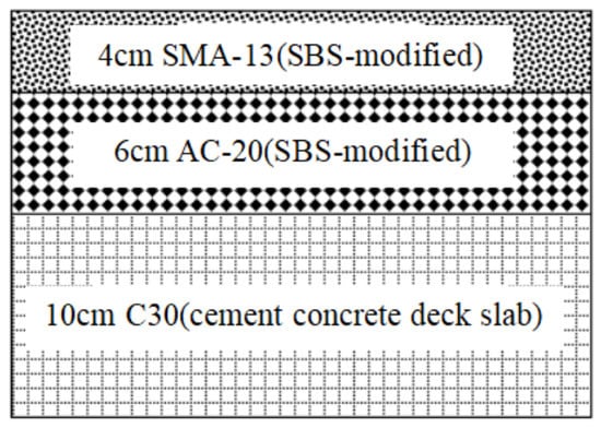
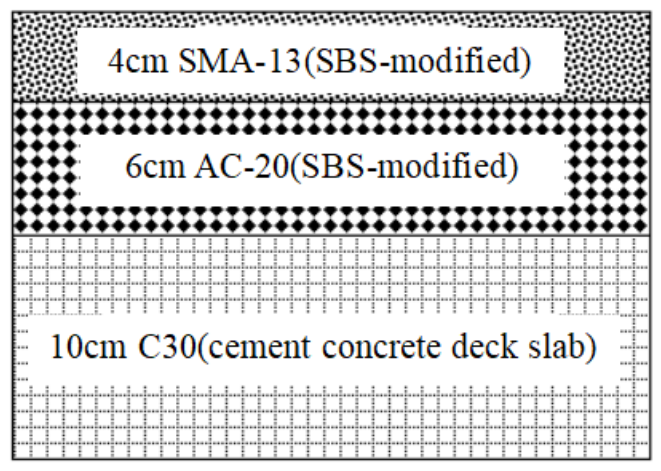
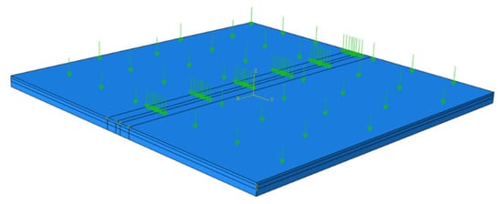
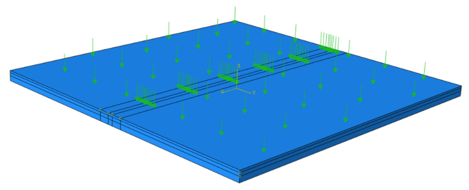
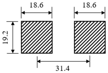
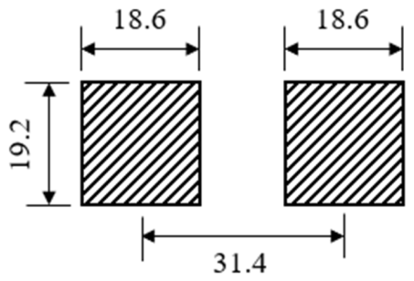
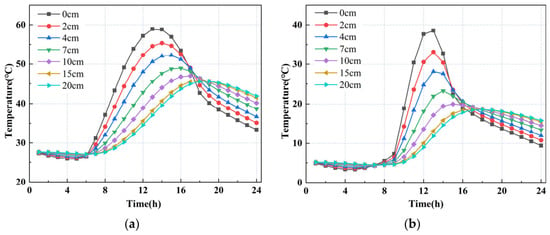
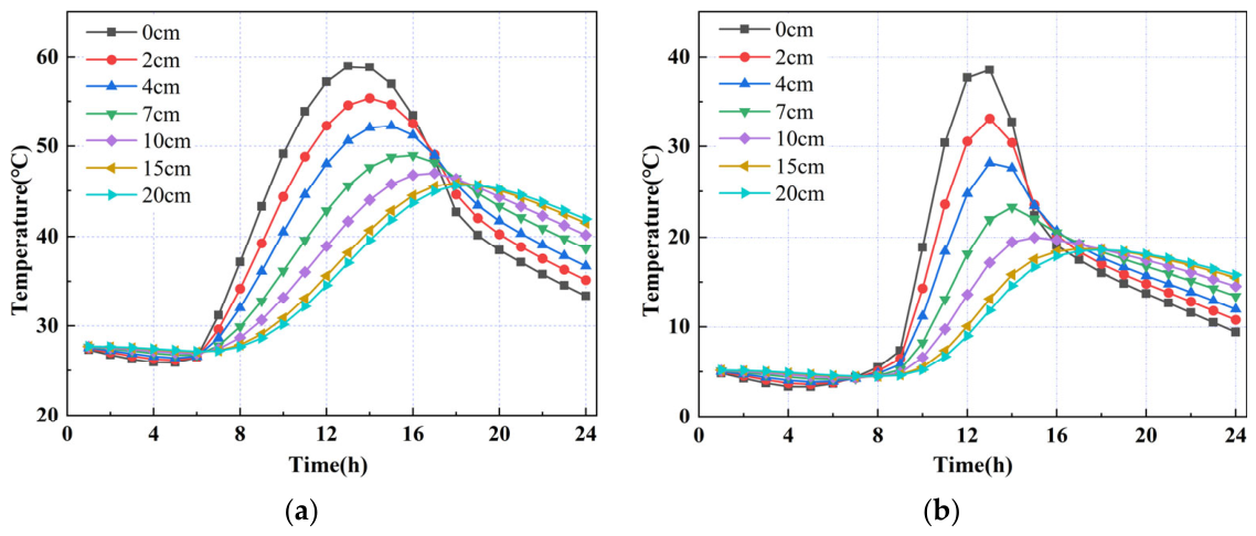
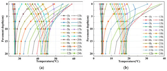
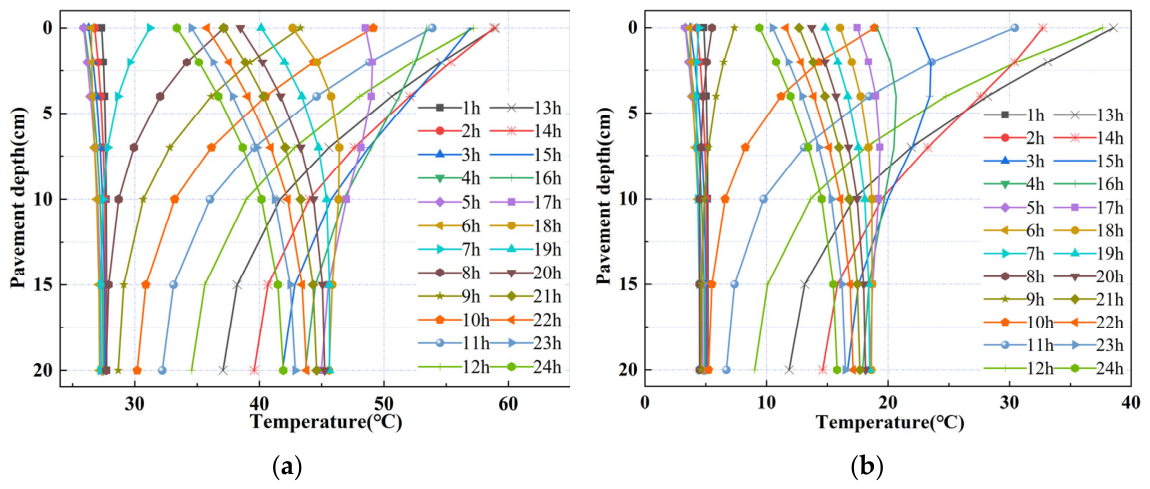
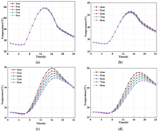
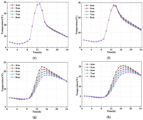
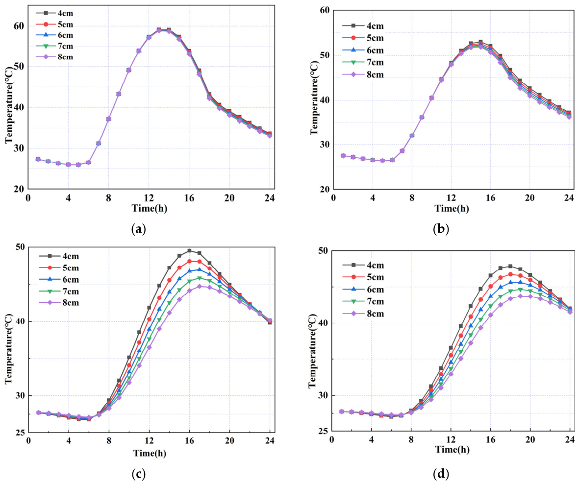
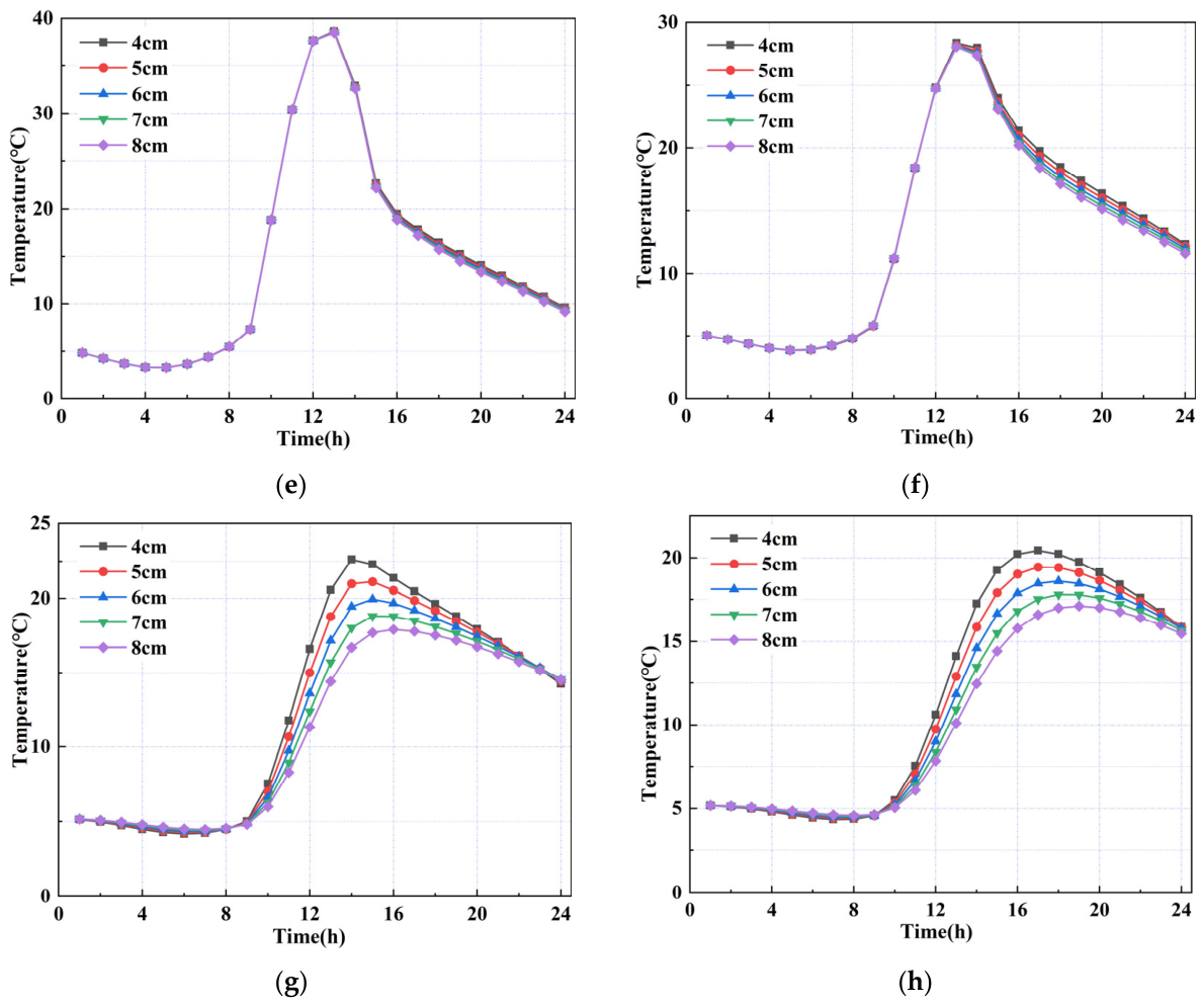
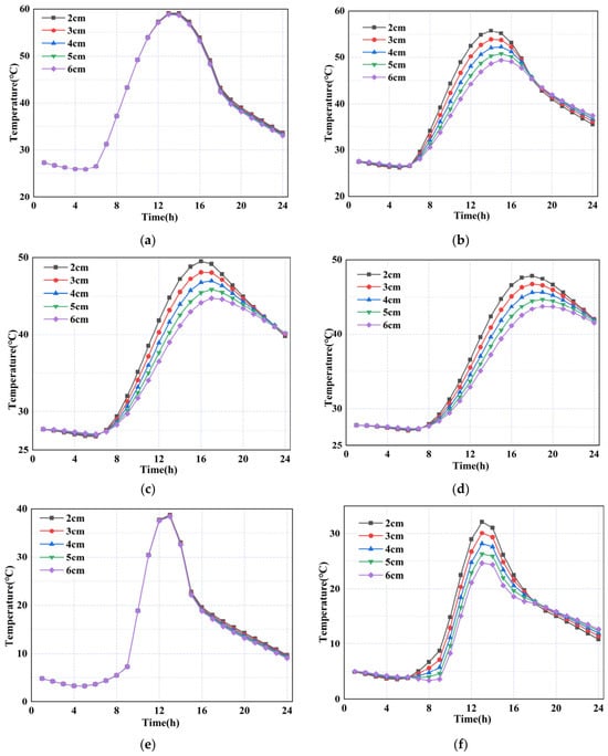
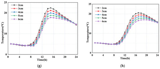
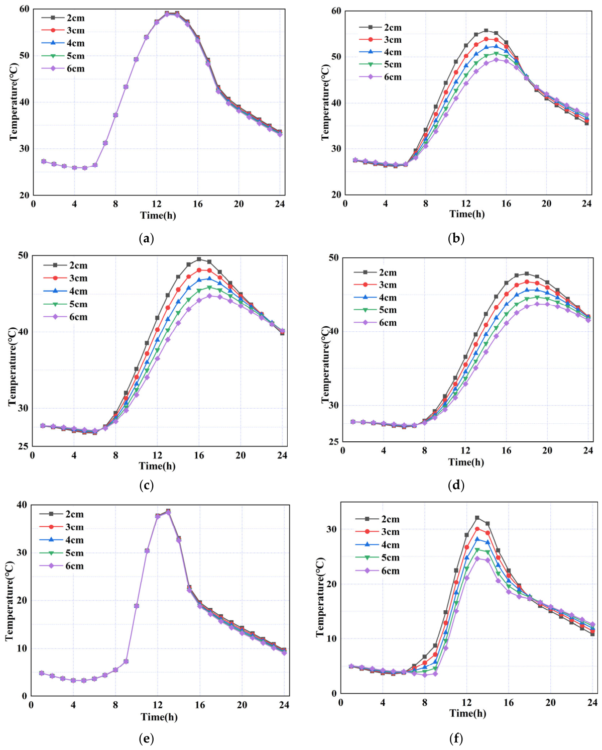
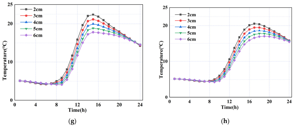
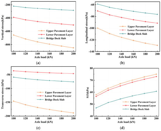
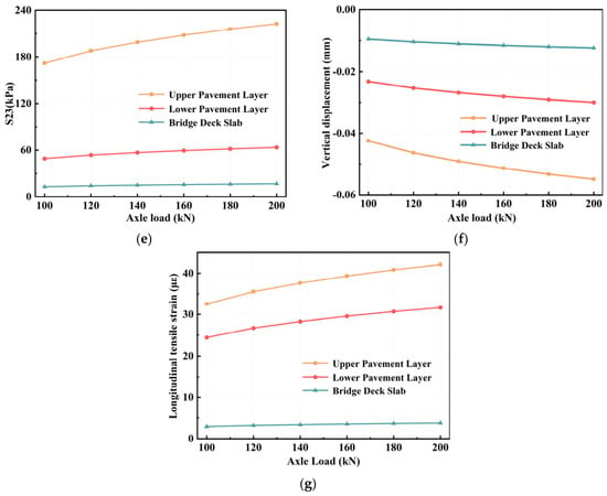
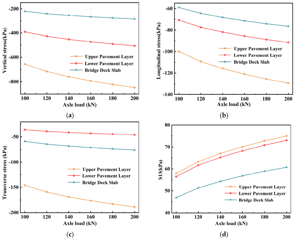
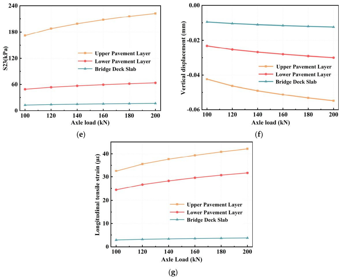
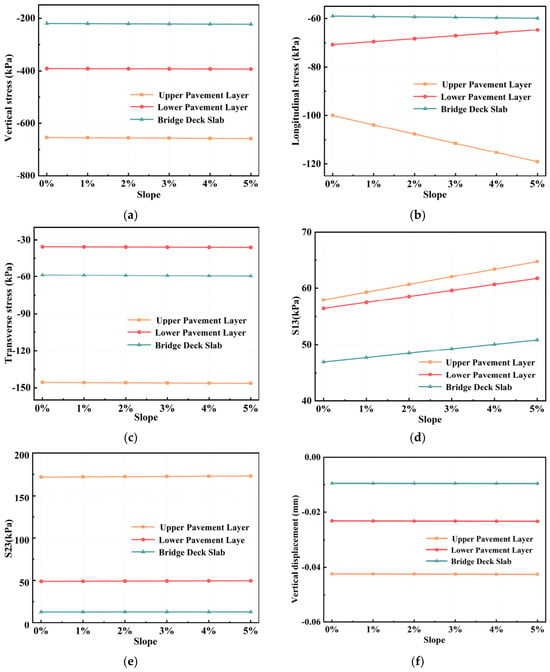
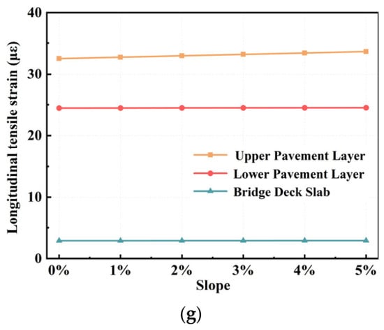
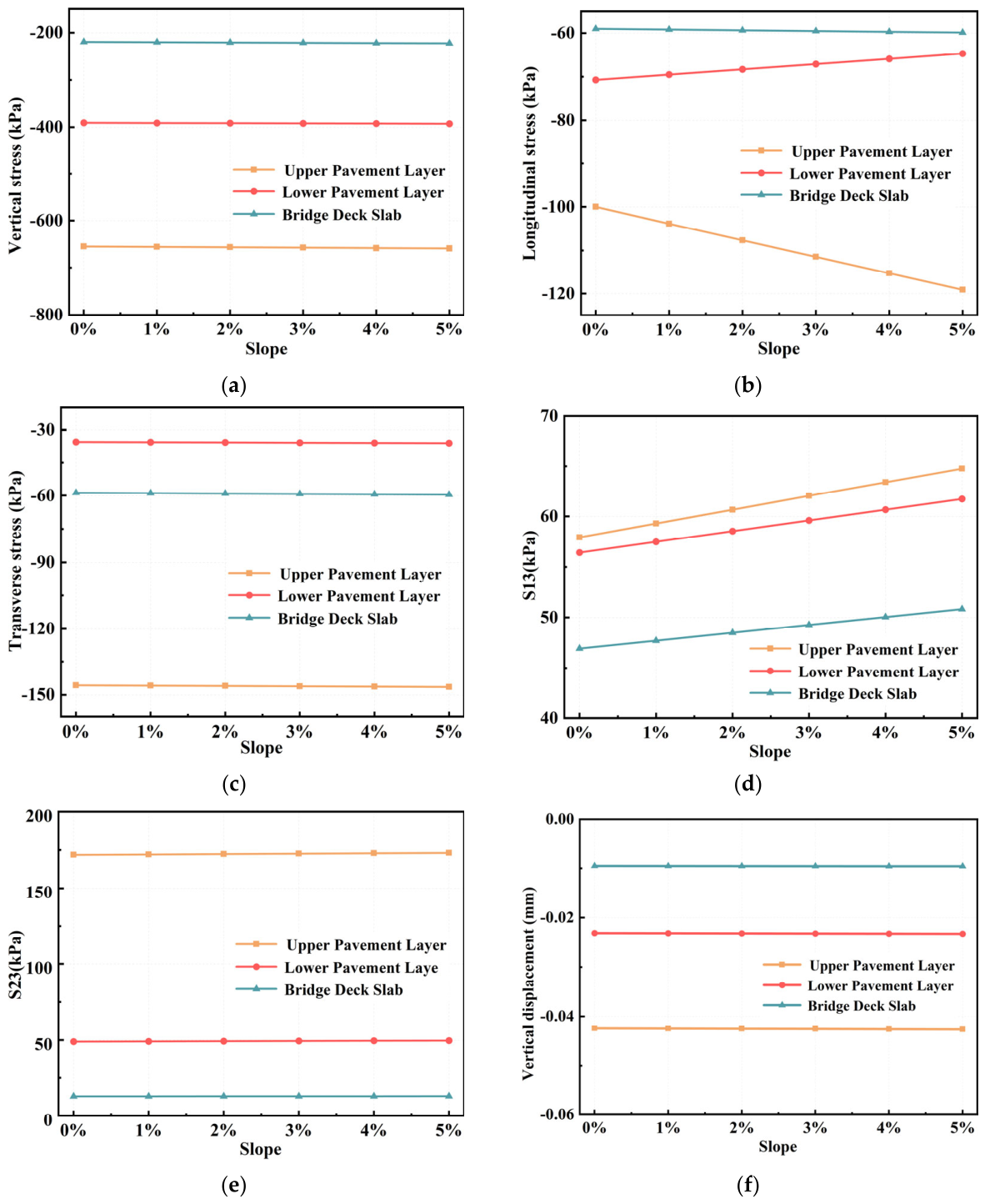
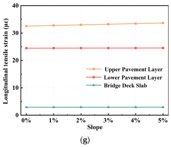
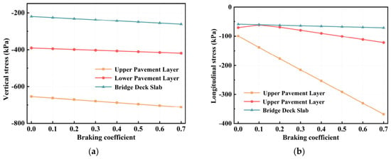
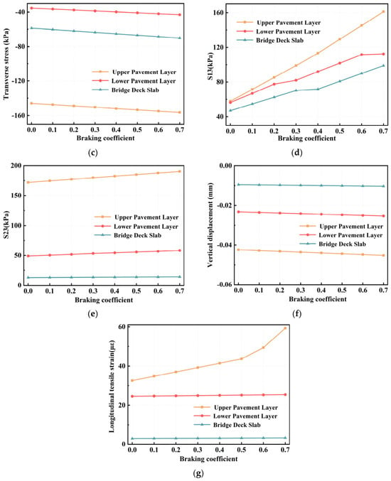
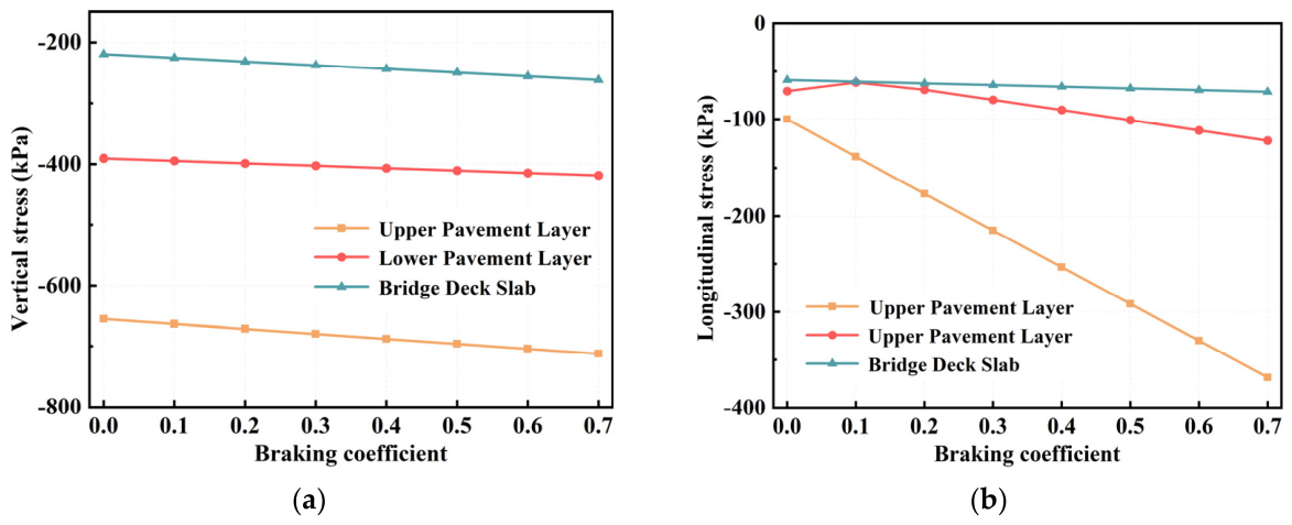
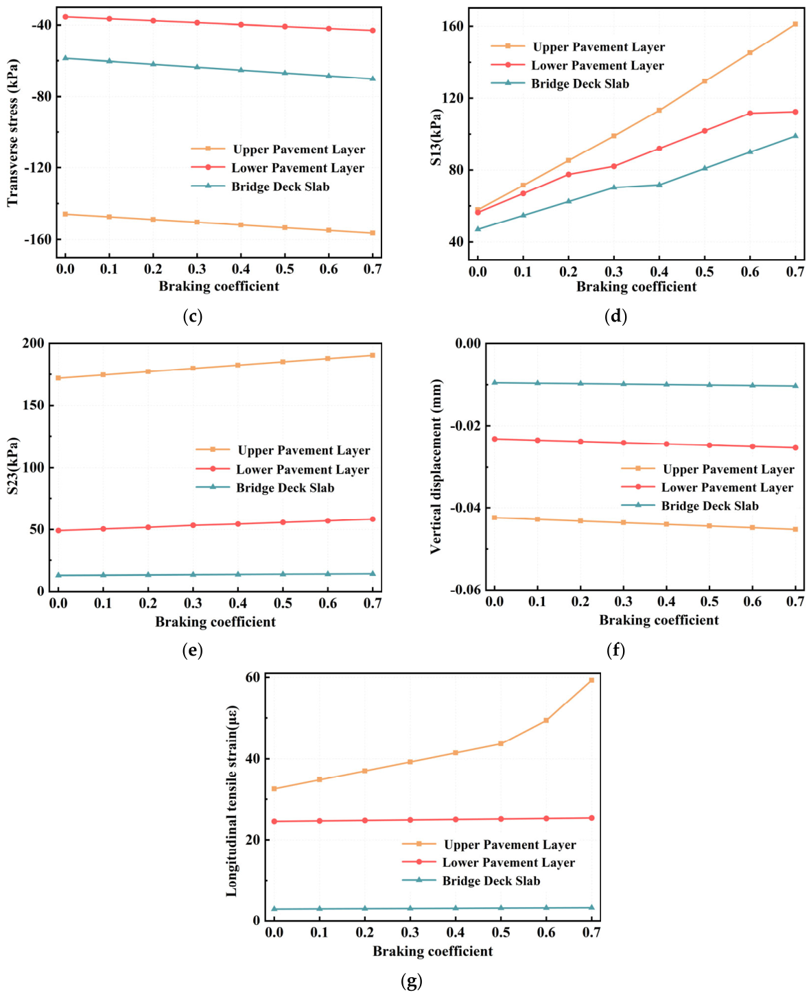
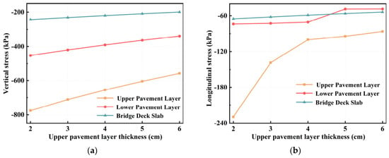
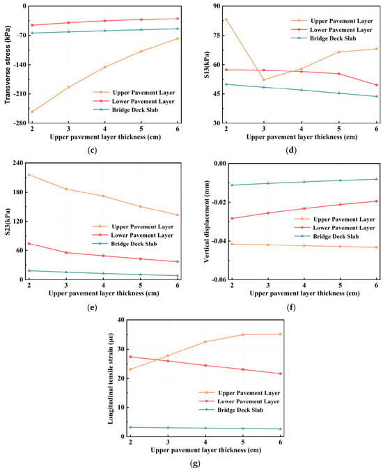
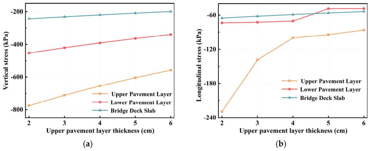
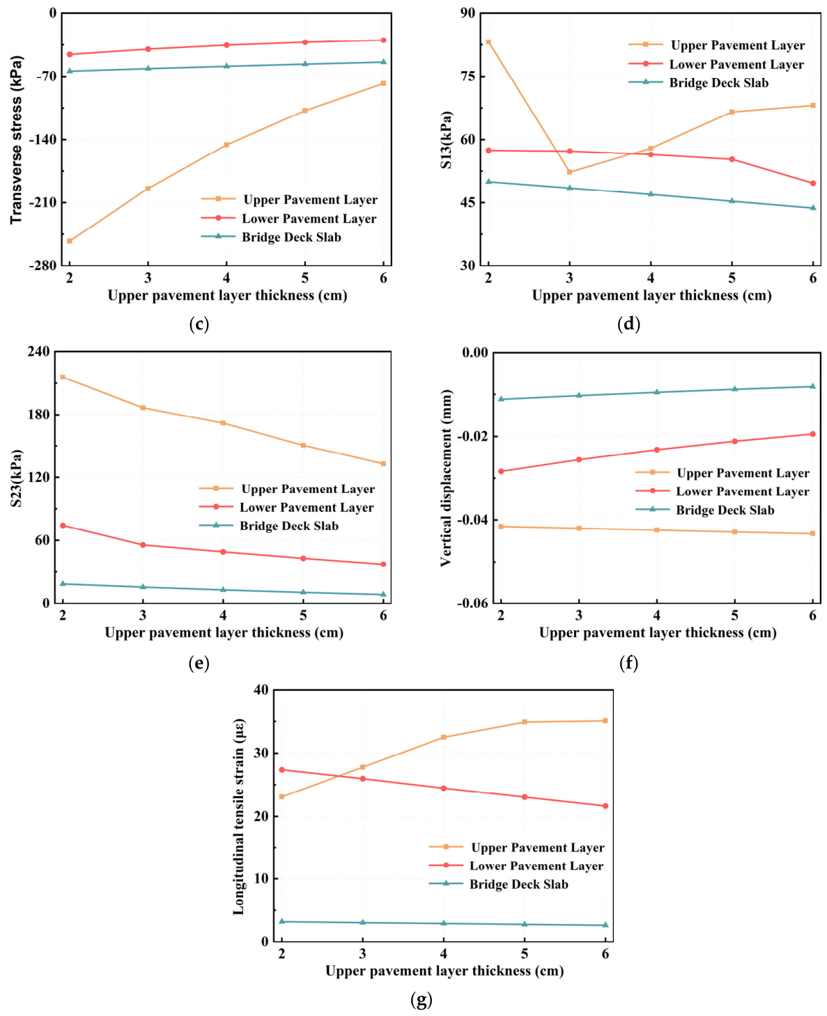
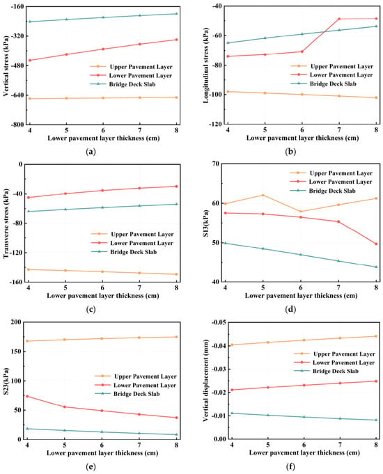
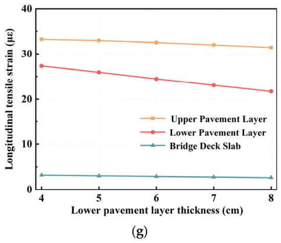
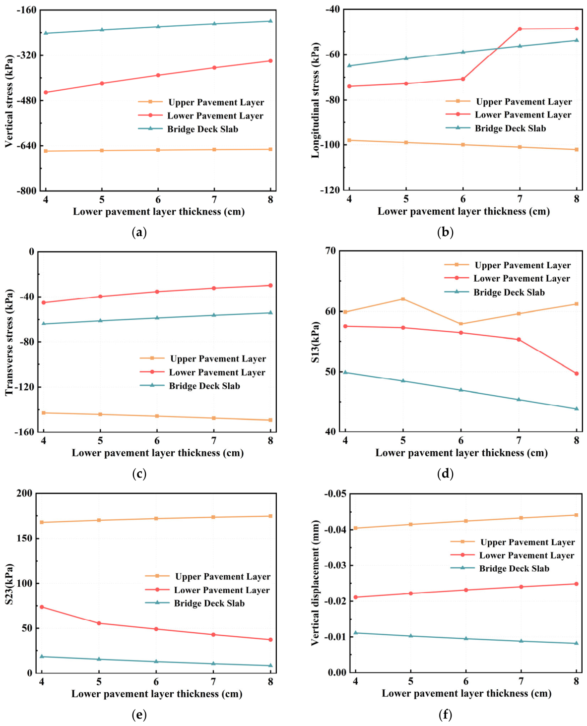
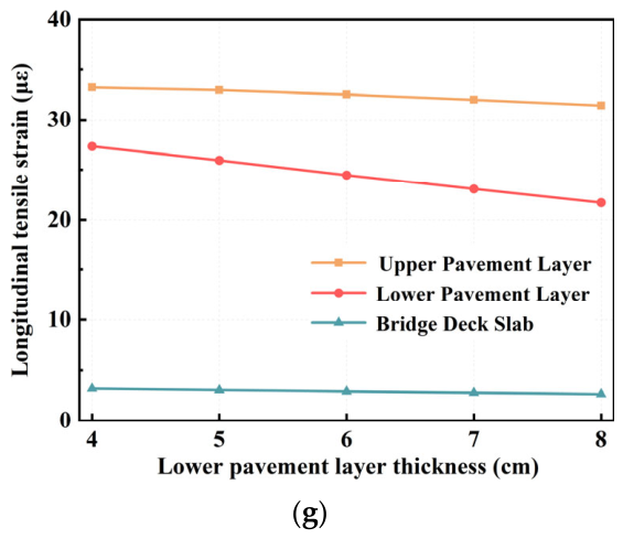

Disclaimer/Publisher’s Note: The statements, opinions and data contained in all publications are solely those of the individual author(s) and contributor(s) and not of MDPI and/or the editor(s). MDPI and/or the editor(s) disclaim responsibility for any injury to people or property resulting from any ideas, methods, instructions or products referred to in the content. |
© 2026 by the authors. Licensee MDPI, Basel, Switzerland. This article is an open access article distributed under the terms and conditions of the Creative Commons Attribution (CC BY) license.