


Abstract
Analog, paper-based workflows remain the norm in the condition assessment of reinforced concrete infrastructure, limiting the efficiency with which diagnostic data can be used in maintenance planning. In this research, a pre-processing procedure and BIM implementation workflow for half-cell potential measurement data are proposed, implemented in open-source software, to enable data-efficient integration of diagnostic information into a BIM model. By interpreting the potential mappings as point clouds, areas relevant for maintenance planning are automatically identified through the analysis of geometric features. These identified areas are subsequently transformed into BIM objects that carry the relevant diagnostic information. The results demonstrate that the pre-processing procedure and BIM implementation workflow reduce the number of required BIM objects by over 98% (from 27,040 to 434 elements) and the IFC file size by 97% (from 77.8 MB to 2.3 MB), enabling a lightweight BIM implementation with substantially improved rendering performance.
1. Introduction
Deterioration of reinforced concrete structures across Europe in recent decades is largely attributed to durability-related deficiencies [1]. Traffic infrastructure—including bridges, tunnels, and parking structures—is exposed to particularly aggressive environmental conditions, leading to accelerated deterioration and increased demands on maintenance management [2]. One of the most harmful environmental effects is the ingress of chlorides (primarily from de-icing salts) into the concrete, which initiates reinforcement corrosion. This process results in concrete cracks and spalling, thereby compromising traffic safety and, in severe cases, the structural load-bearing capacity. Consequently, the service life of the affected structures is significantly reduced [3]. To enable need-based maintenance strategies, the corrosion state must be assessed—including the identification of areas where corrosion is likely or already active. For this purpose, Non-Destructive Testing (NDT) methods such as half-cell potential measurements are routinely applied.
Currently, building diagnostics and condition assessment rely predominantly on analog, paper-based workflows. At the same time, there is a growing need for efficient assessment of existing infrastructure [4], which calls for a digital solution achievable through Building Information Modeling (BIM). Three-dimensional building models enriched with diagnostic data can support more informed and efficient maintenance planning. However, full-surface half-cell potential surveys of large structural elements can yield tens of thousands of individual measurement points. Existing implementation approaches [5,6] produce a large number of BIM objects, potentially overloading the model. Therefore, more efficient approaches to integrating such data into the BIM model are required.
2. Background
2.1. BIM and Maintenance Planning
Extending the service life of existing structures is essential in the context of resource scarcity, as maintenance is generally more sustainable than new construction [7]. However, as the building stock ages, the lack of complete and up-to-date documentation complicates maintenance and repair planning [8,9]. Globally, interest in applying BIM to infrastructure projects has grown considerably [10]. While BIM is now widely adopted in the design and construction of new structures, its integration into maintenance and repair processes remains limited [5].
A major challenge in applying BIM to maintenance planning is that current manual planning processes, regulatory frameworks, and diagnostic devices are not designed for this purpose. For example, BIM authoring software does not provide native functionality for maintenance planning tasks, such as integrating diagnostic data into the model. Therefore, custom solutions are necessary. Several such approaches have been proposed to integrate NDT data into BIM models. NDT integration approaches fall into two categories: those that embed measurement data directly within the BIM model and those that link the model to an external database. When NDT data are integrated directly into the BIM model, the applied strategies depend on the type of measurement. Various studies [4,5,6,11] focus on the integration of diagnostic data by generating dedicated BIM objects to carry the measurement information. Investigated NDT methods include concrete cover measurements, ground-penetrating radar (GPR), and half-cell potential measurements. A common characteristic of these approaches is that each individual measurement value is represented by a separate BIM object, often resulting in a large number of elements. Simple geometric shapes, such as spheres or rectangular tiles, are typically used for three-dimensional representation, while the diagnostic information is stored as object properties. As a consequence, BIM models integrating full-surface half-cell potential surveys can contain tens of thousands of individual diagnostic elements, posing challenges for model performance and usability.
2.2. The Open BIM Approach and Industry Foundation Classes
The use of open standards, such as the Industry Foundation Classes (IFC), enables the exchange of BIM information across various platforms [12]. According to [13], the IFC format is considered the de facto standard for open BIM. It enables the structured description of geometry, properties, and relationships within a building model. In the IFC schema, an entity represents a real-world object, an entity type (also called a class) serves as a template to create entities, and entities have attributes assigned to them that describe their properties or condition characteristics [14]. Standard properties and condition characteristics of entities are defined within the IFC schema; however, non-standardized attributes are excluded. These attributes are referred to as dynamic attributes. Dynamic attributes can be freely created using the subclass IfcProperty and are grouped into an IfcPropertySet. Analogously, the IfcProxy allows for the dynamic definition of custom entities. These extensions provide a wide range of possible applications for the IFC schema, including its use in maintenance planning.
IFC operations—including geometry creation, property assignment, and entity management—can be automated via the IfcOpenShell Python API [15,16]. A standard method for representing three-dimensional geometry in solid modeling is the Boundary Representation Method (BRep) [14]. With the mesh representation functionality implemented in the IfcOpenShell API, it is possible to create complex geometries in IFC based on the BRep concept using Python code.
2.3. Basics of the Half-Cell Potential Measurement and Current Research
Half-cell potential measurement is an established NDT method for locating actively corroding reinforcement and is typically used to detect chloride-induced corrosion. Chlorides act as catalysts to the corrosion process, facilitating the breakdown of the passive oxide layer on reinforcement [17]. Because this occurs without an overall decrease in pH, chloride-induced corrosion typically results in localized corrosion zones [18]. Identifying such areas is a prerequisite for targeted maintenance planning. After the corrosion process of the reinforcement is initiated, the difference between the electrochemical potentials of actively corroding and passive areas produces a potential field within the concrete, driven by the resulting corrosion current. This potential field can be detected on the concrete surface using half-cell potential measurements, allowing the identification of actively corroding reinforcement.
For comprehensive, full-surface assessment of corrosion likelihood, an inspection is conducted by qualified testing personnel. First, the reinforcement layout is identified in order to define a measurement grid for assessing the corrosion likelihood. The potential mapping is performed using specialized devices equipped with a movable reference electrode, e.g., a wheel electrode. Using these devices, the component surface can be scanned along the predefined measurement grid. Ionic contact is ensured by the wheel electrode via a wetted sponge surrounding the wheel and by moistening the concrete surface, while the reference electrode is electrically connected to a reinforcement connection point at the component. Most scanning devices are additionally equipped with electrical displacement transducers to record the spatial position of measured potential values and enable subsequent planar mapping.
ASTM C876 [19] recommends threshold values for interpreting the results of half-cell potential measurements. Although these criteria are commonly applied in practice, they provide only rough guidance and should not be interpreted as absolute indicators of the electrochemical condition of reinforcement steel in concrete, as discussed in [20]. In its passive state, the potential of reinforcement is not a fixed value but depends on various factors. As a result, a single measured potential value is insufficient to reliably determine whether active corrosion is occurring or not [18]. Instead, the entire potential mapping must be evaluated holistically. The technical leaflet B 03 by the German Society for Non-Destructive Testing [18] recommends interpreting potential mappings by calculating the potential gradients across the concrete surface. Distinct potential gradients indicate a high probability of active corrosion at the respective location. Nevertheless, in practice, the graphical representation of potential mappings by color-coding the values based on their potential is typically preferred for a quick evaluation, as it is a simple and effective tool for visualizing corrosion activity. Usually, color scales comprising three to four base colors [18] are used to clearly differentiate between varying potential values. A gradation interval of roughly 50 mV is commonly applied, which facilitates the quick identification of conspicuous potential funnels. At the center of such potential funnels, the potential is typically more than 100 mV lower than in the surrounding areas.
Recent research has focused on quantitative methods for the analysis of half-cell potential measurement data. Statistical approaches have been proposed for deriving threshold potentials and updating service life predictions based on the distribution of measured values [21]. While these approaches provide valuable support for the quantitative assessment of corrosion likelihood, the question of how to efficiently integrate the resulting diagnostic information into BIM models for maintenance planning remains largely unaddressed.
The present work addresses this gap by focusing on the automated classification of potential mappings into planning-relevant and non-relevant areas—emulating an expert’s initial visual assessment—and on the subsequent data-efficient BIM implementation of the identified areas.
2.4. Point Cloud Processing with Geometric Features
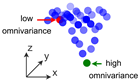
A point cloud is defined as a set of points (x, y, z), each representing a location in three-dimensional space. By applying Principal Component Analysis (PCA) to point cloud data, eigenvectors and eigenvalues can be extracted, providing insights into the local shape of the surface [22]. From these eigenvectors and eigenvalues, specific geometric features can be derived [23], which characterize different aspects of the local surface geometry [24]. The geometric feature omnivariance quantifies the irregularity of the spatial distribution of points within a local neighborhood [23]. Low omnivariance values typically correspond to points on flat surfaces, whereas high values are associated with rougher, more irregular surfaces [25]. Since omnivariance is calculated based on a predefined number of nearest neighbors around a point of interest, the choice of neighborhood size significantly influences the estimation of this attribute, introducing the risk of oversampling [25]. CloudCompare is an open-source software platform for point cloud analysis that supports, among other functions, PCA-based geometric feature extraction including omnivariance [22,26].
3. Development of the Pre-Processing Procedure and BIM Implementation Workflow
3.1. Objectives and Design Principles
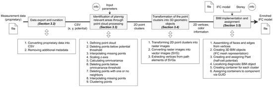
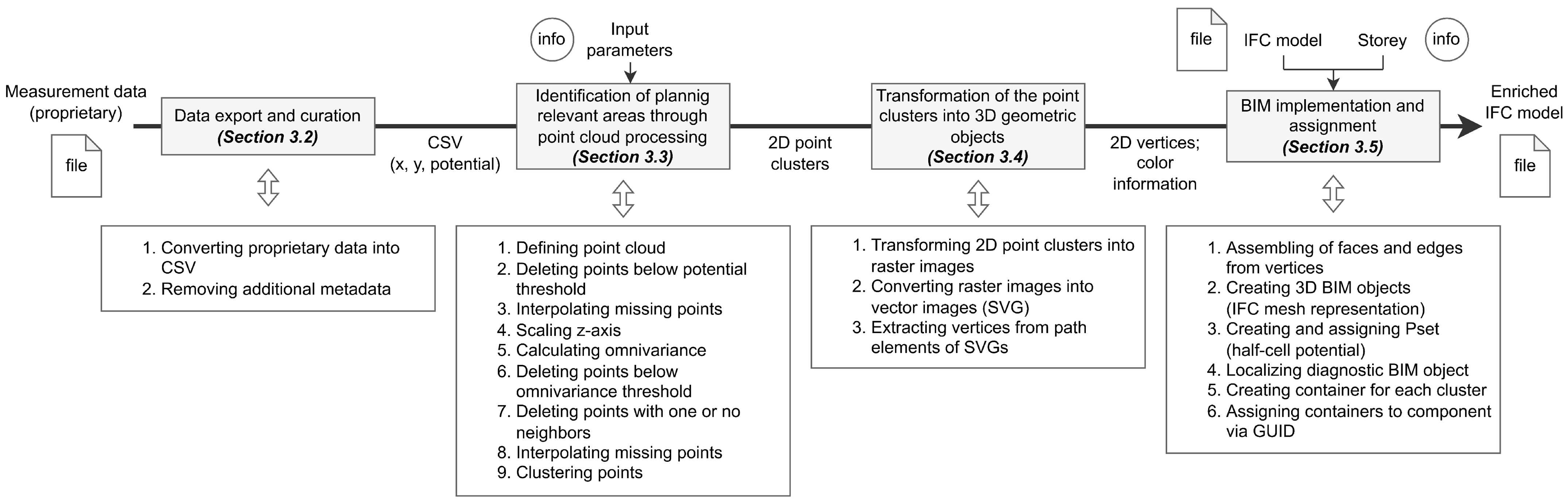
The method developed in this work consists of four main steps. First, the half-cell potential measurement data are exported and curated. Second, the data are interpreted as a point cloud and analyzed with respect to omnivariance to identify areas suspected to be of higher relevance for maintenance planning. Third, subregions within these areas that exhibit similar potential values are grouped and automatically transformed into three-dimensional geometric objects. Finally, these objects are implemented in the BIM model and enriched with the diagnostic information. An overview of the proposed workflow is provided in Figure 1.
Figure 1.
Workflow of the automated pre-processing procedure and BIM implementation workflow of half-cell potential measurements.
Following the open BIM approach, open-source software is employed to ensure accessibility and to avoid dependencies on proprietary tools. The Python programming language was chosen to automate the steps. CloudCompare (v2.13.2) and IfcOpenShell (0.8.3.post1) both provide Python wrappers—CloudComPy and the IfcOpenShell API, respectively—enabling their core functions to be integrated into a unified, automated Python workflow. CloudComPy-based point cloud processing was performed in Python 3.10.13, while the remaining workflow components used Python 3.11.11.
3.2. Data Export and Curation
The data obtained from half-cell potential measurements are often stored in proprietary formats. To enable further processing, the data must be converted into an open and readable format, such as Comma-Separated Values (CSV), using the manufacturer’s software. The exported CSV file usually contains additional metadata beyond the essential measurement values, such as device settings, the date and time of measurement, and the device’s name and serial number. This metadata is not required for the subsequent processing steps and is therefore excluded from the working dataset. The original exported file, including all metadata, is retained and remains available for reference, as it may be relevant for interpreting the measurement results. After this cleaning process, only a list of the spatial coordinates (x and y positions) and the related measured potential values remain. This cleaned dataset is then used as input for the pre-processing procedure.
3.3. Identification of Planning-Relevant Areas Through Point Cloud Processing
As noted in the literature, distinct gradients resulting from significant changes in surface geometry may indicate potential funnels corresponding to areas with a higher corrosion likelihood [18]. While experts often identify these geometric changes visually and on a qualitative basis, this work aims to identify them using geometric features. By interpreting the potential values as z-coordinates of the point cloud, the potential mapping is transformed into a scalable three-dimensional surface geometry. As a result, a connection is established between the electrochemical information and the surface topography. During the development of the workflow, several geometric features were examined: anisotropy, dip/gradient, eigentropy, normal change rate, planarity, surface density, surface variation, and omnivariance. The latter feature, which describes the irregularity of the surface geometry (see Section 2.4), showed the highest capability for identifying relevant regions within the potential mapping, particularly the potential funnels. Consequently, omnivariance was investigated in greater detail.
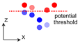
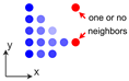
In this research, the Python wrapper CloudComPy [26] was used to automate the functionalities of CloudCompare (v2.13.2), in particular, the calculation of omnivariance. The pre-processing requires the definition of four input parameters. These include the potential threshold, which is used to remove potential values above a specified limit; the scaling factor for the z-axis of the point cloud, which is necessary to balance the spatial dimensions in x–y and z direction, since the measured potential values are given in mV and therefore differ in magnitude from the x- and y-coordinates given in meters; the neighborhood radius, which is required for the calculation of omnivariance (see Section 2.4); and the omnivariance threshold, which is used to remove areas of the potential mapping whose surface roughness is below a specified value. The various steps of the pre-processing are summarized in Table 1.
Table 1.
Overview of the pre-processing steps.
3.4. Transformation of the Point Clusters into Three-Dimensional Geometric Objects
The point clusters, colorized according to their potential, were transformed into raster images. The position of each cluster, relative to the local coordinate system used to perform the potential mapping, was temporarily stored for later use. Each point within a cluster corresponds to a single pixel in the raster image.
The further processing focuses on identifying and grouping areas of uniform color within these raster images, as such zones correspond to similar levels of potentials. Instead of storing color information for each pixel individually, as in raster images, vector graphics group adjacent pixels of the same color and store only the geometric information necessary to describe the boundaries of the geometry.
A widely used open standard for vector graphics is the Scalable Vector Graphics (SVG) format. In SVG, the path element is well-suited for representing arbitrary two-dimensional geometry, as it encodes shape boundaries via a sequence of corner point coordinates. The image processing workflow was implemented in Python using the Python package pixels2svg (v0.2.3) [27].
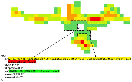
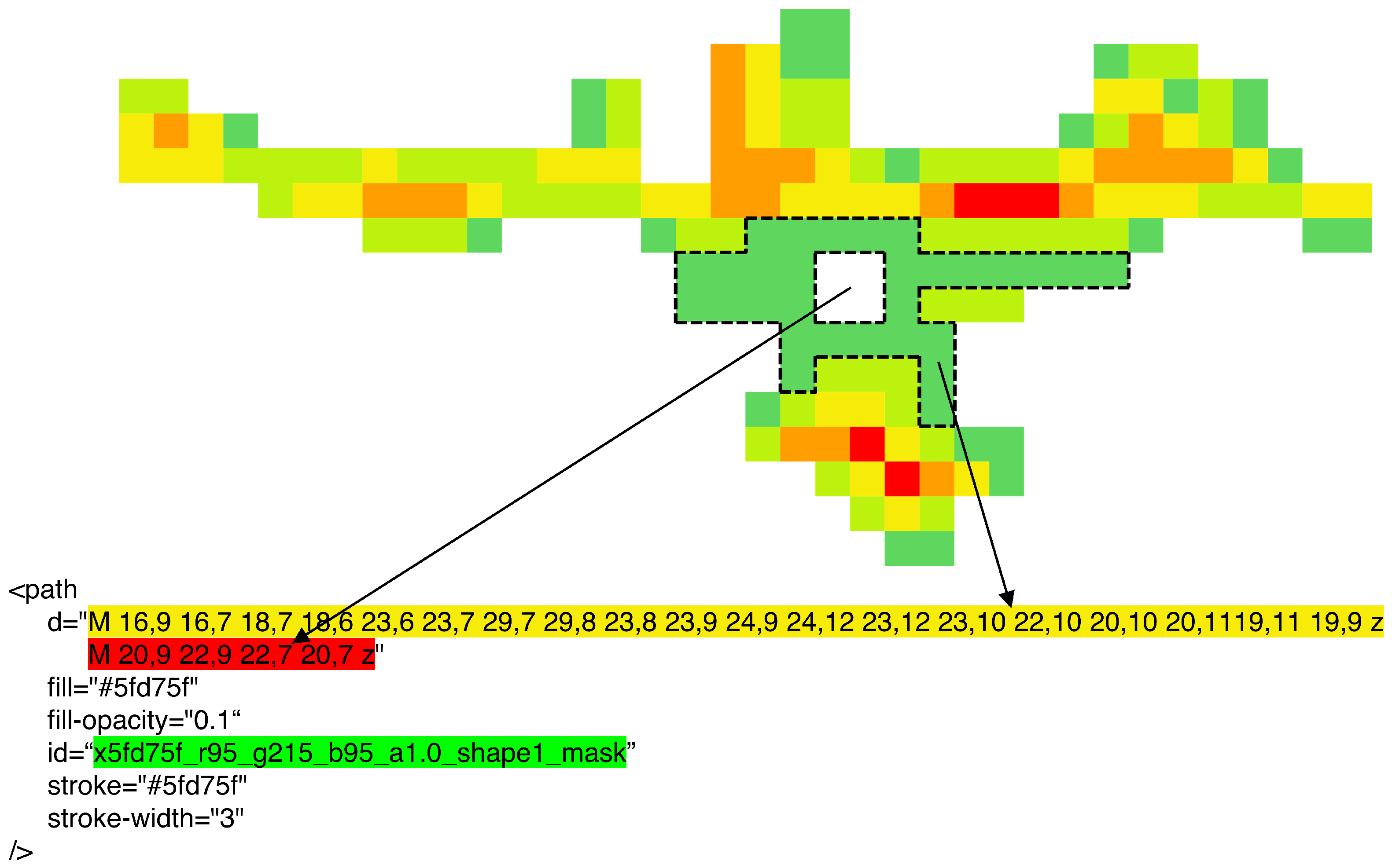
Once the conversion is complete, it is necessary to extract the path elements, including the vertices and associated color information of the elements, from the SVG. Figure 2 illustrates a section of the SVG and the corresponding XML code. In the example, the region outlined in the potential mapping excerpt is represented, with the section marked yellow of the path element containing the coordinates of the outer boundary and the purple highlighted section defining the inner boundary (hole) within the area. The blue marked section contains the rgb-value representing the color of the outlined region. For parsing and processing the SVG data, the Python packages svgelements (1.9.6) [28] and svgpathtools (1.7.2) [29] were used.
Figure 2.
Excerpt of the potential mapping and the corresponding XML code from the SVG file.
3.5. BIM Implementation and Assignment
To generate the three-dimensional geometry, the vertices from the previous step were transformed back to the originally measured raster (100 × 250 mm) and duplicated with an offset along the z-axis, producing a thin volumetric representation of the corresponding potential mapping section. In BRep, each object is described by its vertices, edges, and faces. The assignment of vertices to edges and faces must follow a consecutive and enclosing order to ensure that the resulting geometric representation forms a closed shape.
In this work, the mesh representation functionality of IfcOpenShell, which is founded on the BRep concept, was used to create the diagnostic objects. The class IfcBuildingElementProxy was employed to represent the diagnostic elements, while a specific IfcPropertySet (Pset) named “half-cell potential” was created to store the diagnostic data, in this case, the classes of the measured potential values, derived from the discrete color scale of the potential mapping.
For the correct positioning of the objects inside the BIM model, the temporarily stored positions of the clusters were reapplied. These x- and y-coordinates were transformed into the coordinate system of the BIM model by applying the appropriate offset (translation). Since the z-coordinate is not recorded during half-cell potential measurements, a fixed z-value was manually assigned to all diagnostic objects. This z-value corresponds to the surface elevation of the component within the BIM model where the measurement was taken, with a small offset added to prevent the created diagnostic object from intersecting the component. Once the final coordinates of the vertices were determined, the corresponding IFC entities were generated, and the specific IfcPropertySet was created and linked to each diagnostic object, containing the associated half-cell potential class.
To enhance clarity and usability within the BIM viewer, all entities belonging to the same cluster were grouped into a container entity named “half-cell potential cluster”. This container was then linked to the appropriate building story based on its z-coordinate and the corresponding building element on which the measurement was taken by referencing its Globally Unique IDentifier (GUID).
4. Case Study
This case study applies the pre-processing procedure and BIM implementation workflow to two real-world half-cell potential datasets and evaluates their performance against expert annotations. To systematically evaluate the performance, transferability, and practical applicability of this approach, the investigation is structured into four sequential phases:
- 1.
- Experts in maintenance planning were consulted to identify and mark areas they considered relevant for maintenance planning in two visual representations of potential mappings. The marked areas from all experts were subsequently aggregated and analyzed to assess the consistency of expert judgments.
- 2.
- The developed pre-processing procedure was applied to the first potential mapping using a broad range of input parameter combinations. For each parameter set, the resulting outputs were compared with the expert markings. Based on this comparison, a parameter combination was selected for the next step.
- 3.
- Using the selected parameter combination, the pre-processing procedure was applied to the second potential mapping. The results were evaluated to assess whether the selected parameter combination is transferable to other mappings.
- 4.
- Finally, the BIM implementation workflow was applied. The visualization of the enriched BIM model and the quantification of the resulting data reduction are presented.
4.1. Planning-Relevant Areas of the Potential Mappings Identified by the Experts
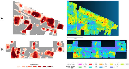
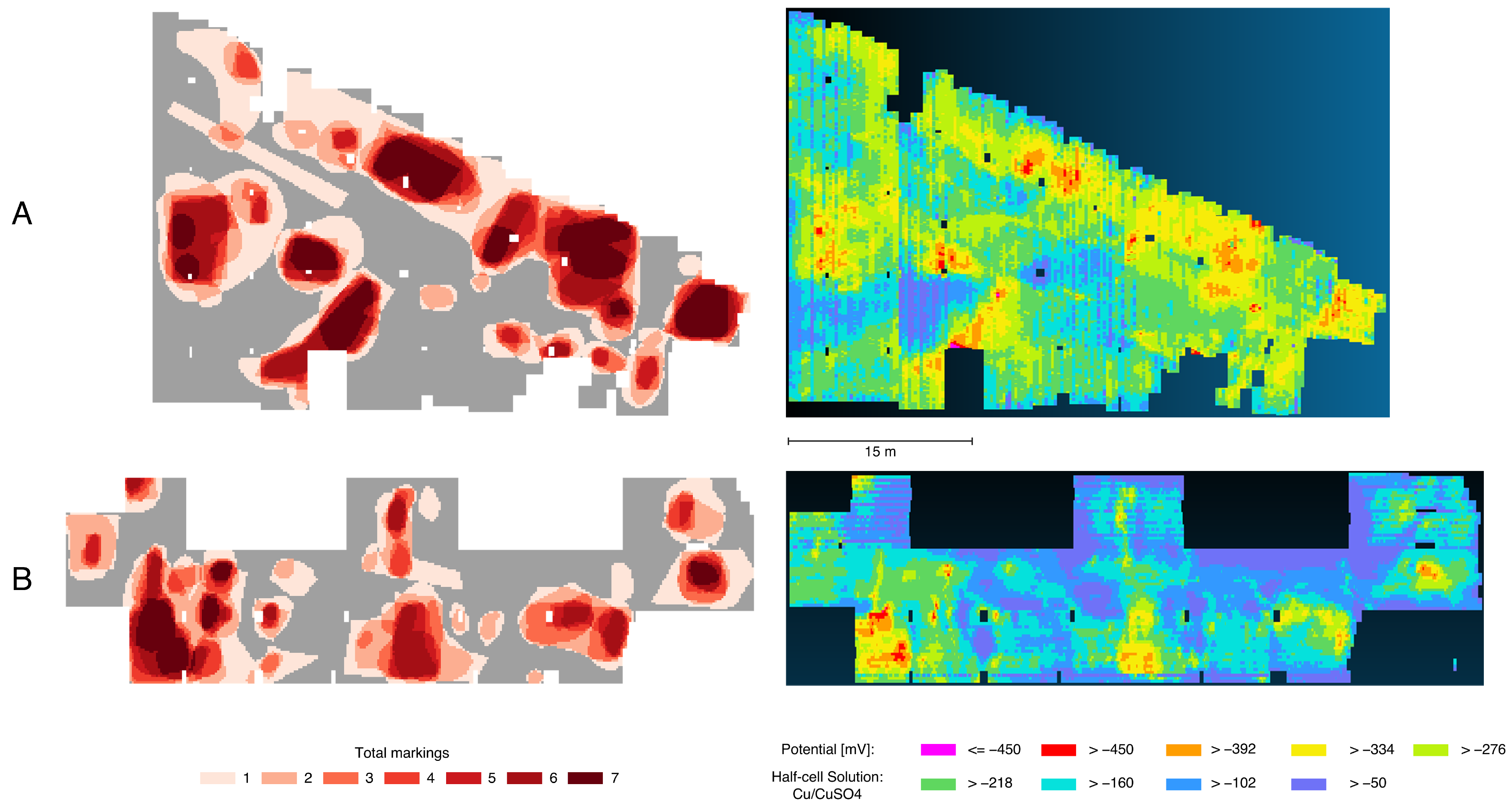
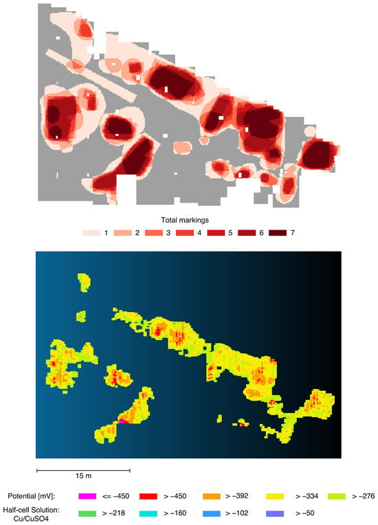
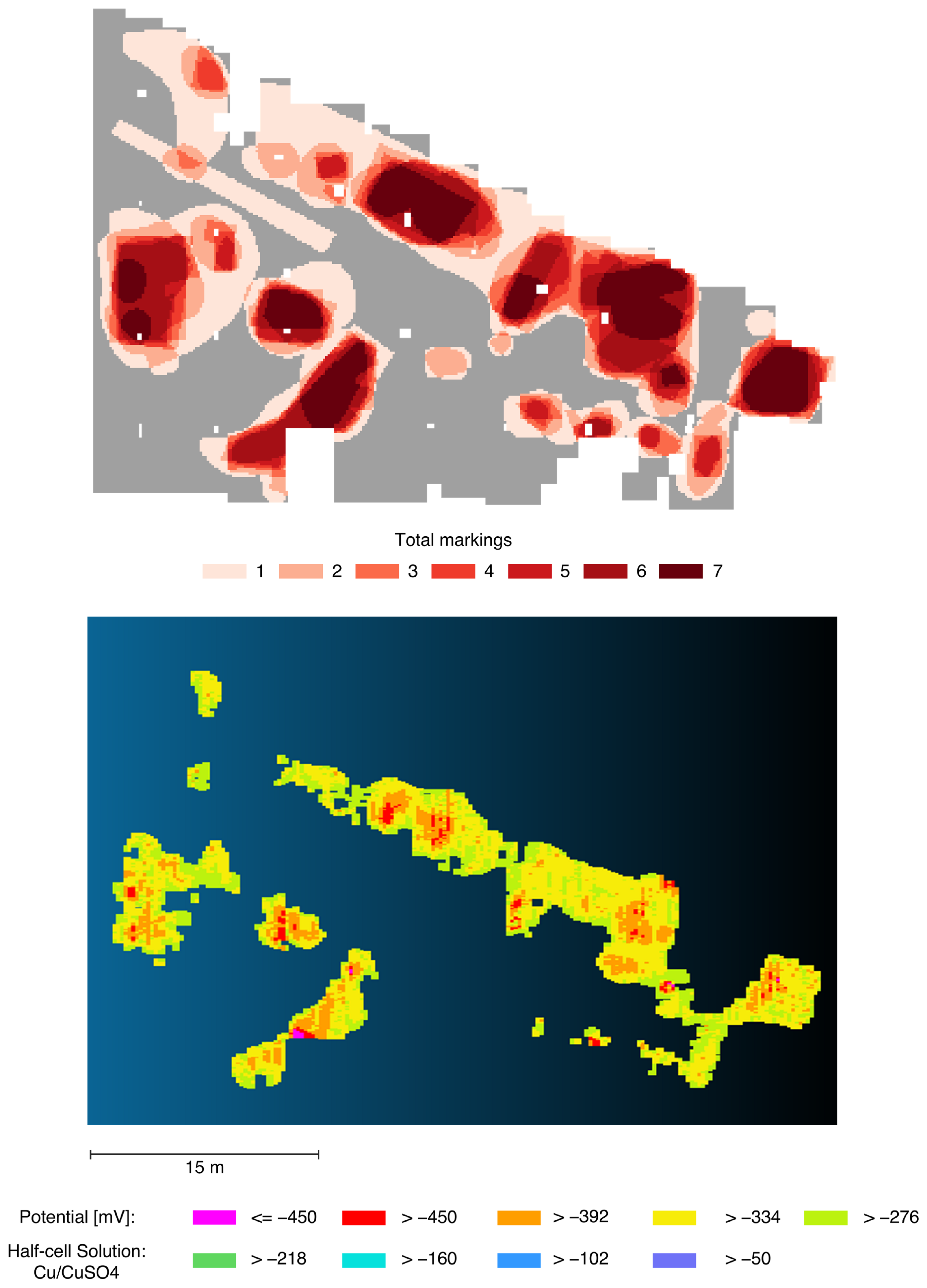
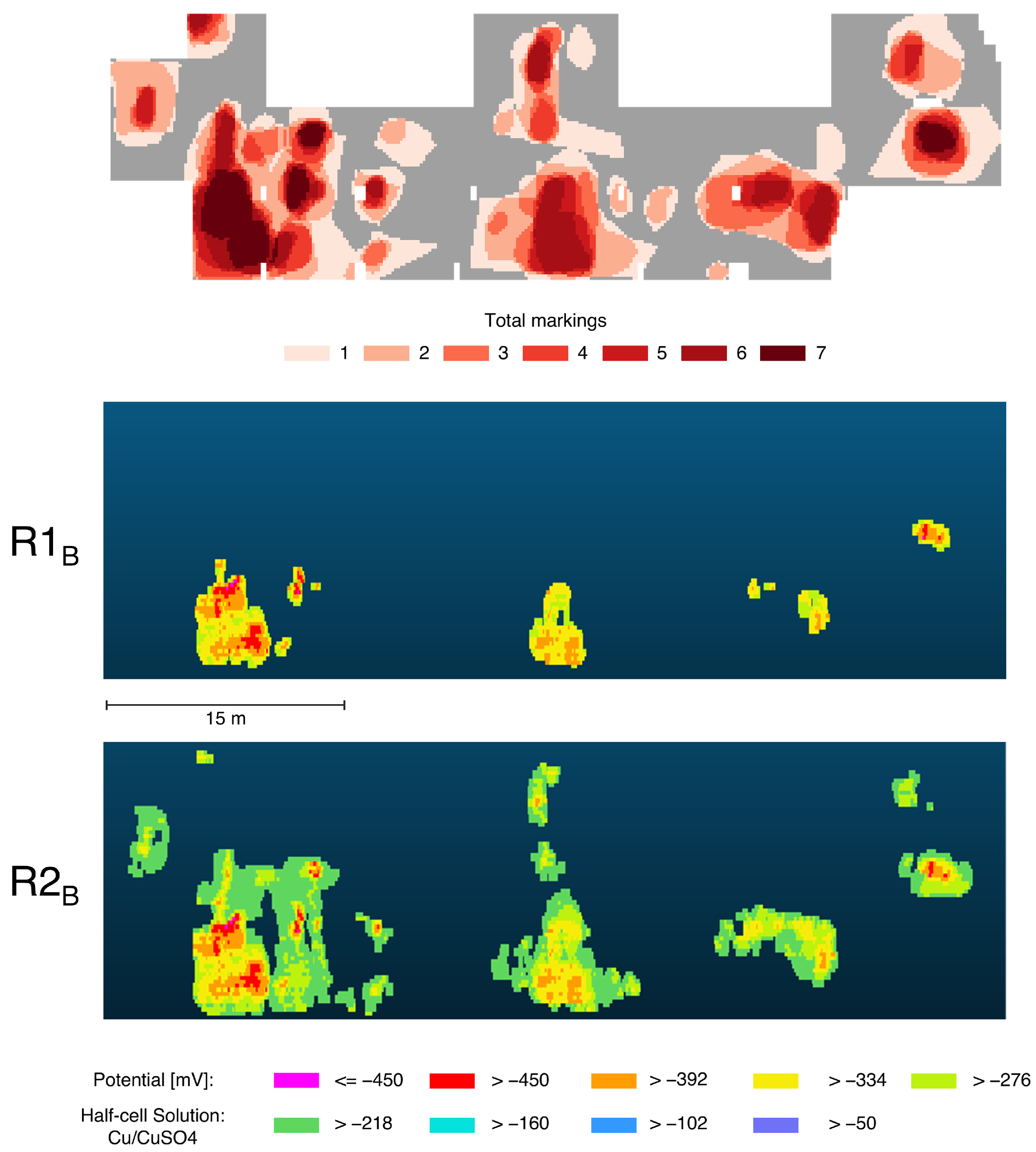
The two datasets used in this study originate from a half-cell potential measurement of a reinforced concrete floor slab and intermediate deck of an underground parking structure and were provided by Raupach Bruns Wolff GmbH (Aachen, Germany). The measured area of the first mapping A covers approximately 950 m2, while the second mapping B covers approximately 680 m2. Both were surveyed on a grid with a spacing of 100 mm in the x-direction (direction of movement) and 250 mm in the y-direction. A half-cell potential measurement device equipped with a four-wheel reference electrode and a Cu/CuSO4 half-cell solution was used for data acquisition. Dataset A consists of 275 line measurements, and Dataset B of 119 line measurements, yielding a total of 38,019 individual measurements for A and 27,040 for B. The visual representations of the half-cell potential mappings are shown in Figure 3. The measurement data were provided as proprietary Profometer Link pqm files (.pqm) and converted into CSV using the manufacturer’s software. Additional metadata were removed, leaving only the spatial coordinates (x and y positions) and the measured potential values.
Figure 3.
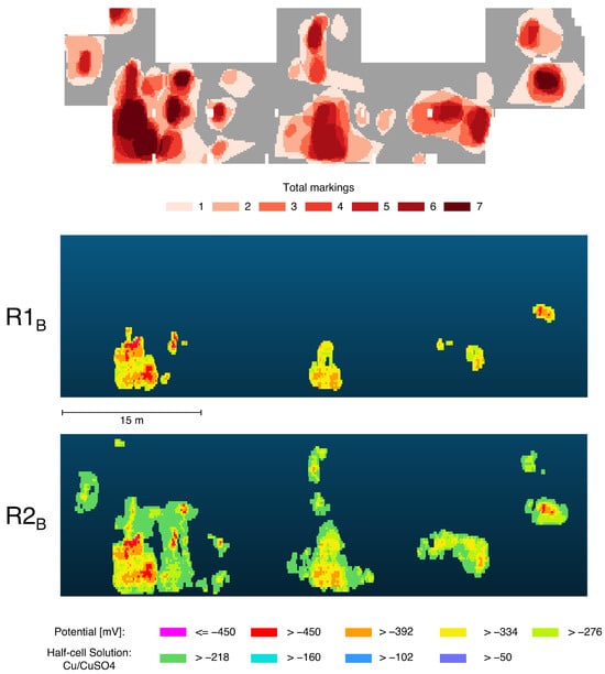
Heat maps (left) of planning-relevant areas of the potential mappings (A,B) (right) identified by the experts.
Eight civil engineering experts (four Dr.-Ing., three M.Sc., one B.Sc.) participated in the evaluation. All are actively employed in condition assessment and maintenance planning, with professional experience ranging from 5 to over 40 years (six experts have 5–10 years; two have ≥20 years). The experts were consulted by email via the authors’ professional network. Six experts evaluated both datasets, while two evaluated only one dataset each, yielding exactly seven independent assessments per dataset. For each potential mapping (A and B), shown on the right side of Figure 3, the seven graphical annotations were overlaid to generate heat maps (Figure 3, left side) visualizing the level of agreement among the experts regarding areas considered relevant for maintenance planning due to an assumed high likelihood of corrosion activity. Darker regions indicate a higher consensus among the participants.
The distribution of the red areas in the heat maps show that a large proportion were selected by only one expert. This accounts for approximately 30% in heat map B and almost 35% in heat map A. Nevertheless, a higher overall level of agreement can be observed in heat map A as the mean of total markings is approximately 3.4, compared to approximately 3.0 for heat map B. This difference can be attributed to the fact that in heat map A a particularly large proportion (approximately 17.1%) was marked by all seven experts, whereas in heat map B only about 7.3% exhibit full agreement. The proportions marked by five and six experts, however, are similar in both heat maps.
4.2. Parameter Study of the Pre-Processing Input Parameters
The input parameters limpot, zscl, r, and limomni influence the results of the pre-processing. Depending on their configuration, more or fewer points are deleted, and the number, shape, and size of clusters (connected components) are affected. To approximate a suitable parameter combination for this use case, a parameter study was conducted. The developed pre-processing procedure was applied to potential mapping A using a wide range of parameter combinations. Based on the experience gained during the development of the procedure, specific parameter intervals were selected, as summarized in Table 2. The scaling factor for the z-axis was fixed at 0.1, as the z-axis scaling and the neighborhood radius are interdependent. In total, potential mapping A was pre-processed using 594 different parameter combinations.
Table 2.
Ranges of the input parameters for the parameter study.
To reduce the impact of inconsistencies among the heat maps on the evaluation of the pre-processing results, a consensus-based ground truth was defined. Only those locations in the heat maps where more than three experts marked the same area were considered. This approach ensures that only regions with a minimum level of agreement are included in the evaluation. Each output of the pre-processing procedure was subsequently evaluated against this ground truth.
The pre-processing procedure aims to classify the potential mapping into areas that are relevant or not relevant for maintenance planning. For each parameter combination, the resulting output point cloud was rasterized into a bitmap using a pixel resolution corresponding to the measurement grid spacing (100 mm × 250 mm) and compared pixel-by-pixel against a binary reference bitmap derived from the expert heat map, with each pixel categorized as true positive (TP), false positive (FP), true negative (TN), or false negative (FN). A true positive represents a point of the potential mapping that is relevant for maintenance planning and was correctly identified as such, and should therefore be maximized. A false positive denotes a point classified as relevant although it is not. While this value should be minimized, false positives are considered less critical, as the incorrect classification remains on the conservative side for planning purposes. A true negative corresponds to a point that is not relevant for planning and was correctly classified, and should also be maximized. In contrast, a false negative indicates a point that is relevant for planning but was classified as not relevant. This type of misclassification is particularly critical, as it leads to the omission of planning-relevant information and should therefore be minimized.
To effectively balance these specific requirements, the F1 score was chosen as the primary evaluation metric. As the harmonic mean of precision and recall, the F1 score inherently penalizes both the critical false negatives (through recall) and the undesirable false positives (through precision). Furthermore, it excludes true negatives from the calculation, preventing the metric from being artificially inflated by a large number of non-relevant background points.
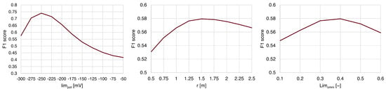
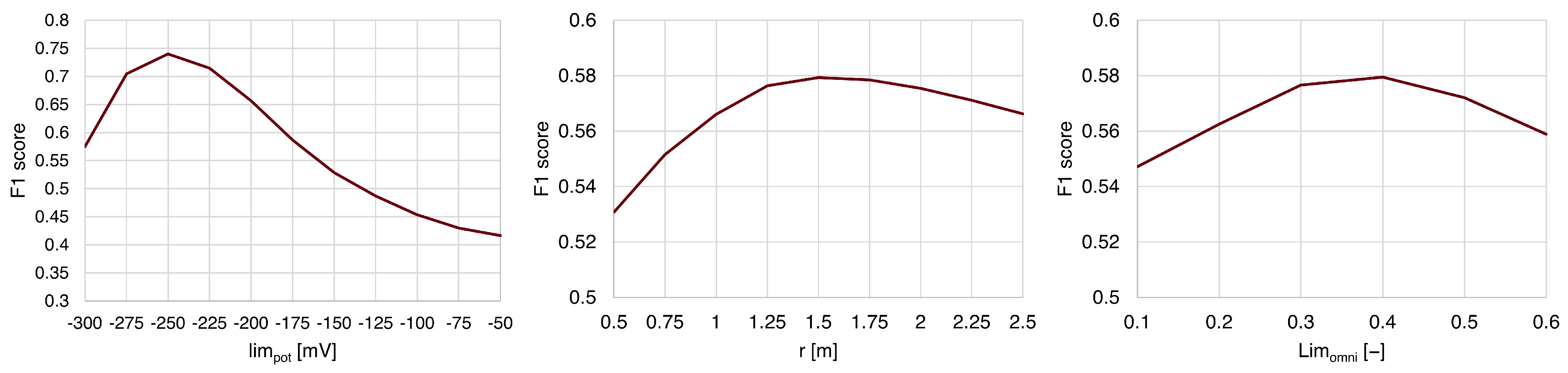
To systematically evaluate the influence of the input parameters on the F1 score, a sensitivity analysis was conducted. In total, 594 pre-processing runs were performed; however, only 534 yielded valid results. This is attributed to the pre-processing failing to produce viable outputs for certain configurations, particularly those involving highly negative values for limpot. For each of these 534 runs the F1 score was calculated. Then each input parameter was investigated separately. The F1 scores of each run with the same value of the investigates input parameter were averaged. Subsequently, this mean F1 score was plotted on the y-axis while the x-axis shows the range of the investigated input parameter to generate the corresponding performance curves. The behavior of the pre-processing in response to each parameter is illustrated in Figure 4. The plot for limpot shows a distinct non-linear effect: the score steadily increases to a peak of 0.740 at a limpot value of −250 mV, before dropping sharply towards −300 mV. In contrast, the plotted curves for r and limomni remain relatively flat, indicating only a marginal effect on the final score.
Figure 4.
Effect of input parameters on the F1 score (empirically averaged over the parameter sample).
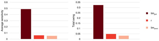
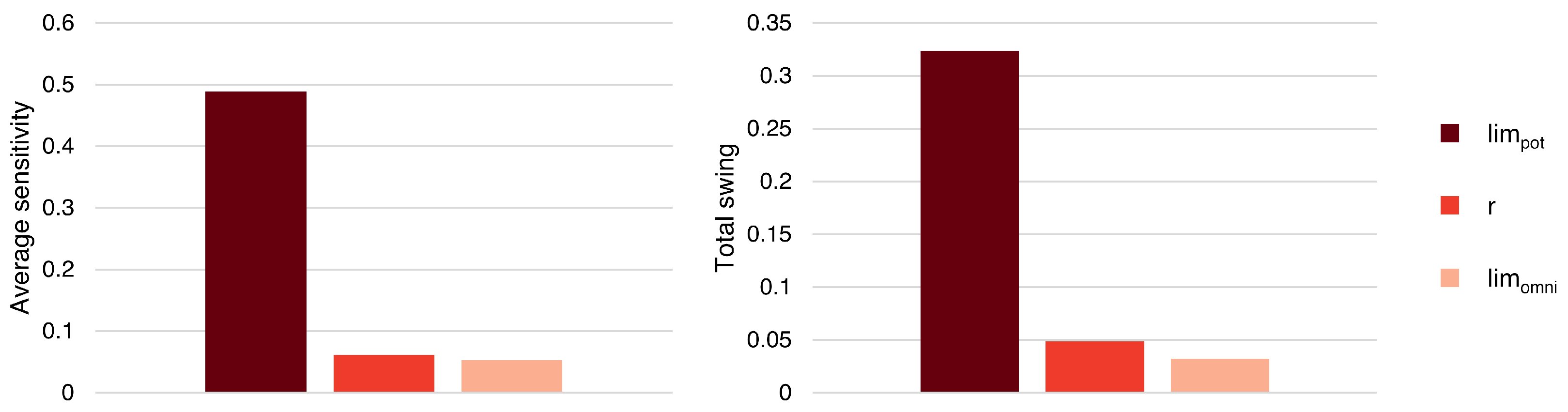
However, because the parameters operate on fundamentally different scales and units, their input ranges were normalized to a dimensionless scale (from 0 to 1) specifically for calculating comparable sensitivity metrics. Based on these normalized ranges, two key comparative metrics were derived: the Total Swing (maximum impact of the F1 score) and the Average Sensitivity (mean absolute gradient). As shown in the corresponding charts in Figure 5, limpot is the primary driver of the pre-processing. It exhibits a Total Swing of 0.324 and an Average Sensitivity of 0.489. The Total Swing for r is merely 0.049 (Average Sensitivity: 0.062), and limomni shows the lowest overall impact with a Total Swing of 0.032 (Average Sensitivity: 0.053). The parameter study demonstrates that the pre-processing is highly sensitive to variations in limpot, whereas r and limomni serve only as minor variables for fine-tuning the results.
Figure 5.
Comparison of parameter sensitivities (Total Swing vs. Average Sensitivity).
To identify a suitable range of parameter combinations, the 95% quantile of the F1 scores was selected, resulting in 27 parameter combinations. The maximum F1 score achieved was 0.783, while the 95% quantile threshold corresponded to an F1 score of 0.757. The distribution of parameters across these 27 combinations is presented in Table 3.
Table 3.
Distribution of pre-processing parameters across the 27 best parameter combinations.
For the potential threshold, a distinct peak can be observed at −250 mV, indicating a strong preference for this value. In contrast, the radius parameter does not exhibit a pronounced peak. Therefore, the midpoint between the most frequent values (1.25 and 1.50), i.e., 1.375, was selected. Similarly, for the omnivariance threshold, the midpoint between 0.2 and 0.3, i.e., 0.25, was chosen.
The resulting parameter combination achieved a true positive rate of approximately 66%, a false positive rate of about 16%, a true negative rate of nearly 99%, and a false negative rate of approximately 21%. The results of the pre-processing using this parameter combination compared with the heat map are presented in Figure 6. Overall, a strong correspondence between the expert-marked areas and the results of the pre-processing can be observed.
Figure 6.
Comparison of the result of the pre-processing of potential mapping A using the selected parameter combination with the heat map.
4.3. Testing of the Selected Parameter Combination
The previously selected parameter combination was subsequently applied to the pre-processing of potential mapping B. However, a visual comparison between the resulting output and the heat map revealed a low degree of agreement (see Figure 7), which was also reflected in the F1 score (0.482). While some hotspots on the heat map were detected, the identified areas were too narrow, and some regions were not covered at all, resulting in the loss of planning-relevant information. Based on the sensitivity analysis, the discrepancies were assumed to result from a potential threshold that was too strongly negative (i.e., −250 mV), which was consequently adjusted toward less negative values. Based on this finding, the two potential datasets were analyzed in more detail. To address the transferability challenge, a data-driven approach for adapting the potential threshold was developed, based on the statistical distribution of the potential values. An examination of the frequency distributions of the potential values of the two potential mappings revealed notable differences. Potential mapping A exhibits a mean potential value of approximately −209 mV with a standard deviation of about 74 mV. The potential threshold used for the pre-processing of potential mapping A corresponds to the 28.5% quantile of this distribution. In contrast, potential mapping B shows a substantially higher mean potential value of approximately −129 mV and a standard deviation of around 82 mV. These differences suggest a relationship between the statistical distribution of the potential values and the appropriate potential threshold to be applied during pre-processing. Under this assumption, the 28.5% quantile was also selected for the pre-processing of potential mapping B, corresponding to a potential threshold of −164 mV.
Figure 7.
Comparison of the results of the pre-processing of potential mapping B using the original parameter combination and the adjusted parameter combination , compared with the heat map.
The results of the pre-processing of potential mapping B using the adjusted threshold are shown in Figure 7, together with the corresponding heat map. Visual inspection indicates a high degree of agreement between the pre-processing results after the adjustment and the heat map, with the primary hotspots now being largely covered. This improvement is equally reflected in the quantitative evaluation of the classification results. While the original parameter combination yields an F1 score of approximately 0.482, the parameter combination with the adjusted threshold achieves a substantially higher F1 score of 0.773. The corresponding performance metrics indicate a true positive rate of nearly 72%, a false positive rate of approximately 29%, a true negative rate of about 98%, and a false negative rate of around 17%.
The results indicate that the potential threshold value is a key adjustment parameter whose influence warrants further investigation. For the subsequent BIM implementation, the results of the pre-processing using the parameter combination incorporating the adjusted potential threshold of −164 mV are used.
4.4. Visualization in a BIM Viewer
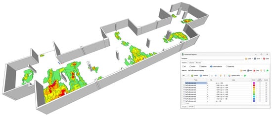
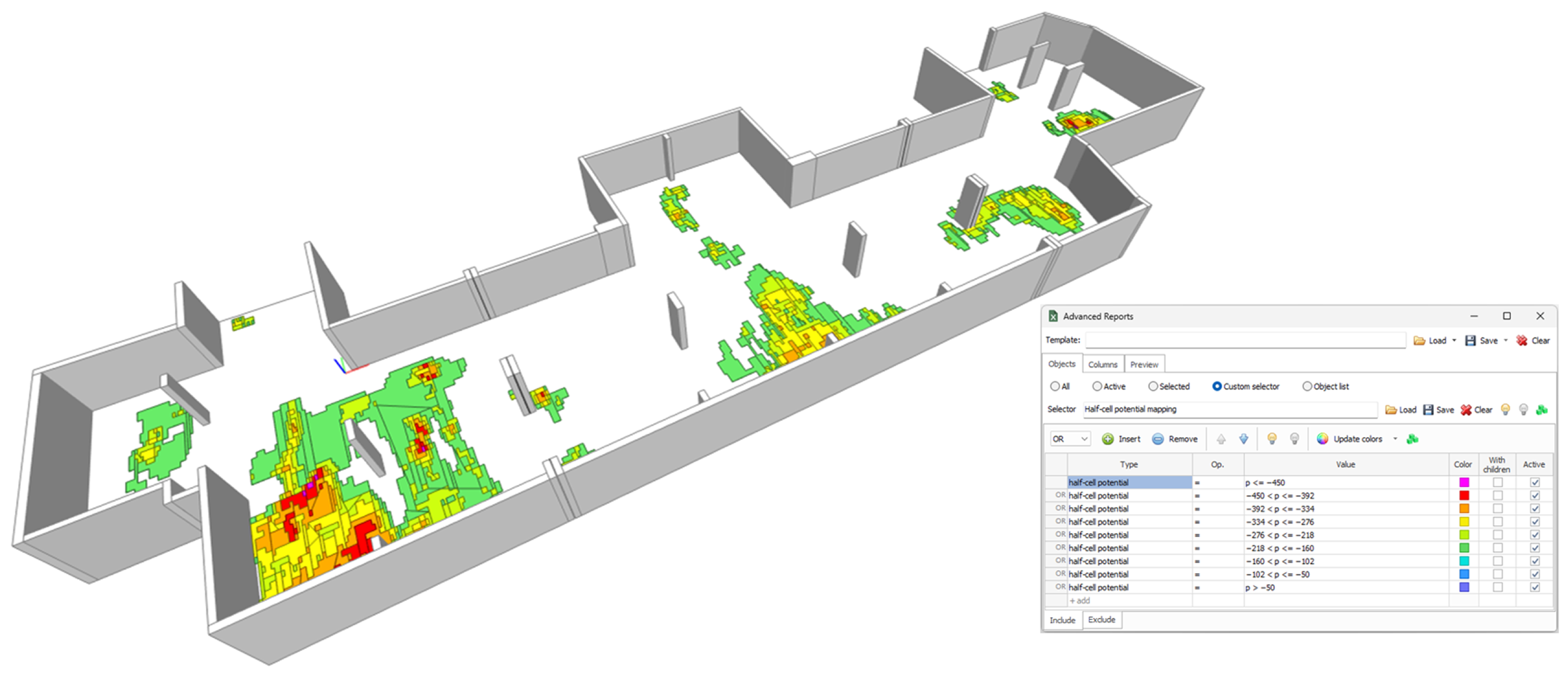
After transforming the point clusters from the pre-processed data of potential mapping B into three-dimensional geometric objects and implementing them into the BIM model, the enriched model can be visualized and analyzed using a BIM viewer. The coloring of the diagnostic objects was performed using the Advanced Reports plug-in for BIMvision. This plug-in enables elements to be colored based on the selected property “half-cell potential”. A screenshot of the resulting visualization in the viewer BIMvision is shown in Figure 8.
Figure 8.
BIM model enriched with pre-processed half-cell potential data, visualized in BIMvision.
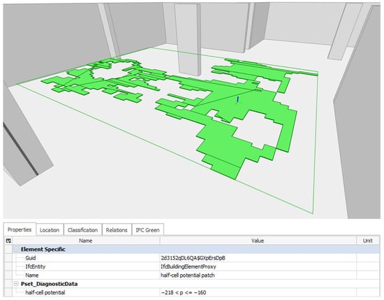
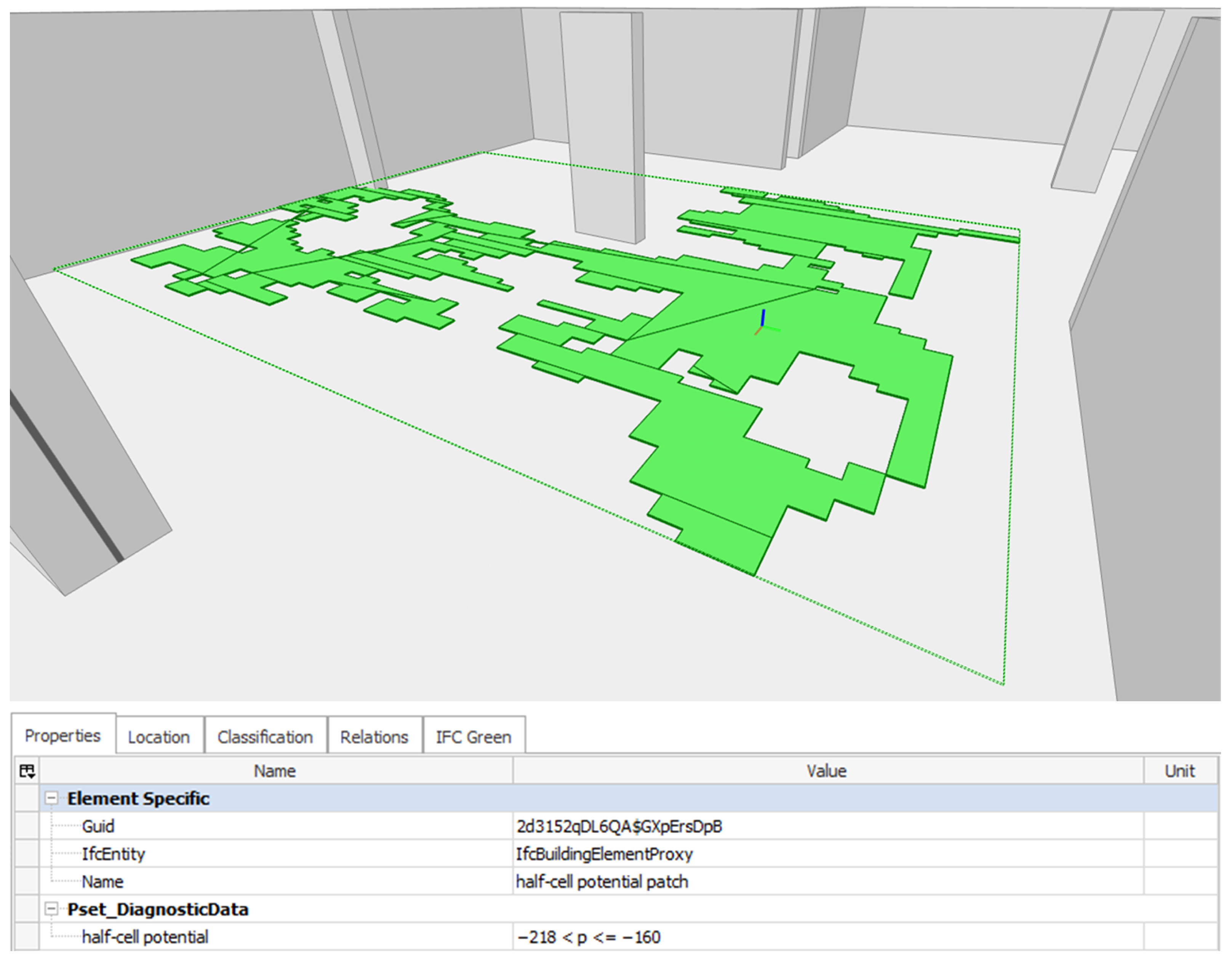
As a result of the SVG transformation, regions exhibiting similar potential levels were grouped into contiguous areas, enabling their representation as single BIM objects. The larger these contiguous areas, the more measured values they contain, and the more storage space can be saved. However, increasing the number of grouped values generally results in greater geometric complexity of the BIM object. Figure 9 shows a complex BIM object representing a large group of values belonging to the class of −218 < p <= −160 [mV]. To improve clarity, the visibility of the other potential mapping BIM objects has been deactivated. This BIM object covers an area of 26.05 m2 and, given the 10 × 25 cm measurement grid, corresponds to 1042 individual half-cell potential measurements. This highlights the efficiency of the BIM implementation workflow and the substantial reduction in the number of required BIM objects to represent the diagnostic data within the BIM model.
Figure 9.
Complex BIM object representing a large excerpt of the potential mapping, visualized in BIMvision.
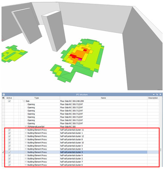
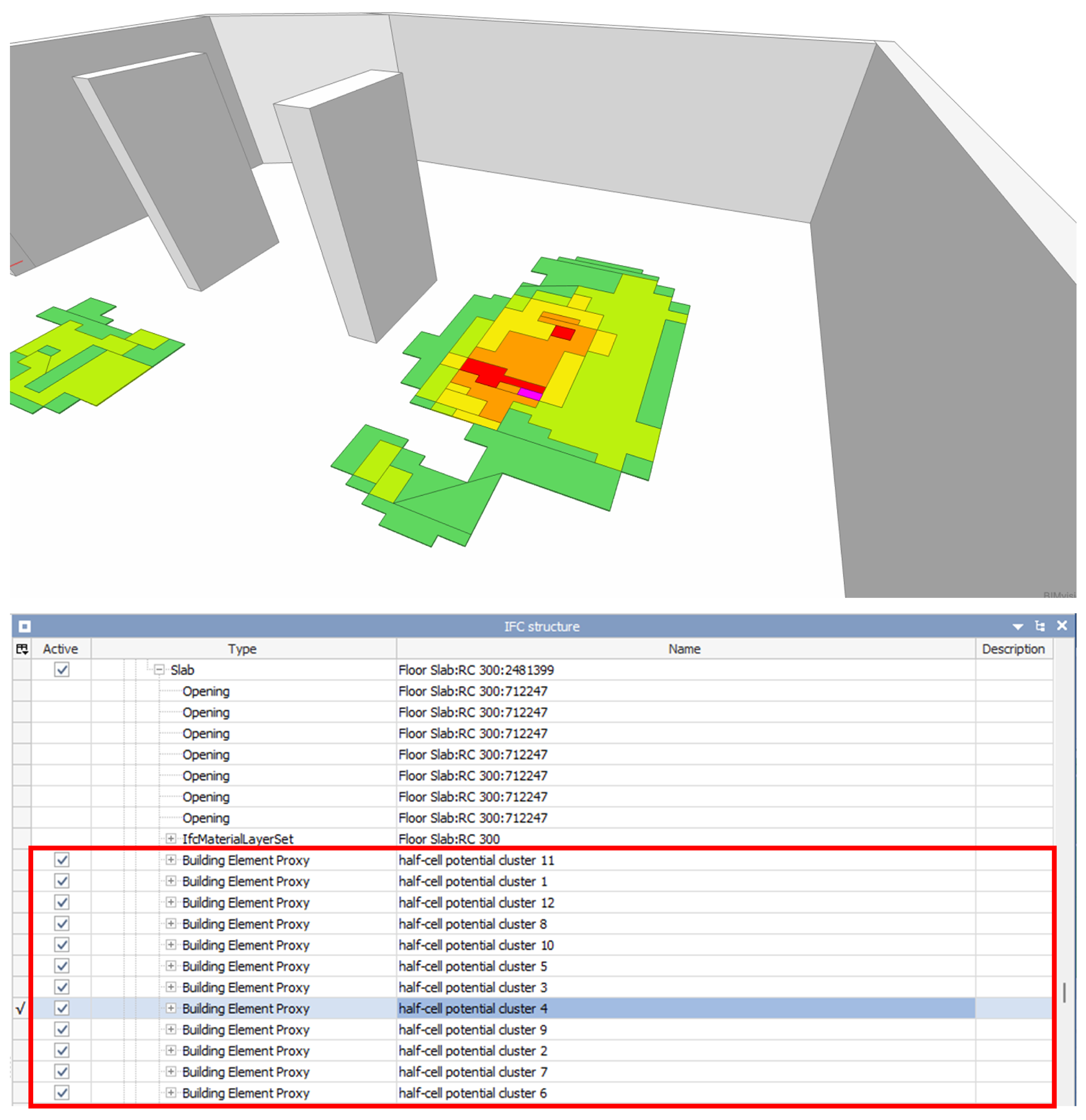
Furthermore, the hierarchical IFC structure (see Figure 10) can be accessed in BIMvision, including the embedded half-cell potential measurement containers (outlined in red). The checkboxes allow users to toggle the visibility of individual containers, enhancing the overall clarity of the visualization. It can also be observed that the diagnostic objects are correctly assigned to the slab element of the underground parking garage.
Figure 10.
A selected potential mapping cluster of the enriched BIM model and an excerpt of the hierarchical IFC structure, visualized in BIMvision.
4.5. Quantification of the Data Reduction
One of the main objectives of the pre-processing and BIM implementation workflow was to significantly reduce the number of required BIM objects to represent the relevant diagnostic information within the BIM model. If the model contains too many individual elements, greater computing power is required for rendering in a BIM viewer, often resulting in degraded rendering performance.
Key indicators of model complexity include the number of vertices, edges, and faces needed to define the geometric objects. Implementing half-cell potential measurements, as performed in [5], would result in each measurement value being represented as a separate BIM object. For the potential mapping investigated in this study, this would translate into more than 27,000 individual diagnostic objects. When using rectangular tile-shaped BIM objects, over 216,000 vertices would be required. After the pre-processing procedure and BIM implementation, the same potential mapping can be represented with 434 elements, corresponding to a reduction of more than 98%. Similarly, the total number of vertices, edges, and faces were reduced by more than 94%. As a result, the data storage required for the representation of the half-cell potential data decreased from 77.83 MB to 2.28 MB, corresponding to a 97% reduction. This reduction in memory usage is achieved by increasing the geometric richness of each diagnostic object. For example, the average number of vertices per element increased from 8 to over 25, and the average number of edges per element increased from 12 to over 35. An overview of these changes is provided in Table 4.
Table 4.
Comparison of storage size and geometric complexity of the diagnostic objects before and after pre-processing.
5. Discussion and Limitations
The pre-processing of the potential mappings does not yield additional insights into corrosion state. Instead, it aims to automatically classify potential mappings into areas that are relevant or irrelevant for maintenance planning, enabling a cluster-oriented BIM implementation for further use. This includes task management via BIM Collaboration Format (BCF) files, automated queries of maintenance-relevant information based on the IFC data structure, and improved data management through the direct linkage of inspection results to their corresponding structural components within the BIM model. By embedding the measurement data in a machine-readable format, planning steps such as the assignment of maintenance tasks can be automated, thereby reducing manual effort and minimizing information loss across the maintenance lifecycle. In combination with the BIM implementation workflow, a lightweight BIM model is thereby enabled. While reducing the storage space required to represent diagnostic data from potential mappings in BIM is not critical for small models, where only a few megabytes can be saved, it becomes highly relevant for very large structures, for example, airport parking garages, where substantially more diagnostic data is generated, potentially saving several hundred megabytes that would otherwise overload the model. Nevertheless, the quality of the results strongly depends on the selected input parameters for the pre-processing. The quantification of the pre-processing results must be interpreted with caution due to the limited number of experts involved in the evaluation. For a more robust and reliable assessment, the sample size should be increased. The results of the parameter study indicate that users with expertise in the electrochemical processes of reinforcement corrosion and maintenance planning are required to validate and select an appropriate parameter combination. While the neighborhood radius and omnivariance threshold appear to be robust across different potential mappings, the potential threshold is more sensitive and requires manual selection based on project-specific requirements prior to pre-processing. This introduces an additional manual intervention step into the workflow. Consequently, the responsibility for creating and assessing the results remains with the user.
As noted, statistical methods exist for deriving threshold potentials from the distribution of measured half-cell potential values [20,30]. Combining such approaches with the omnivariance-based pre-processing may reduce the need for manual calibration of limpot and improve threshold robustness across different structures. While the potential threshold required adaptation to the specific potential mapping under investigation, the remaining input parameters (neighborhood radius and omnivariance threshold) appear to be more robust. The neighborhood radius defines the area of influence for the omnivariance calculation and thus determines the area of the surrounding potential mapping considered when evaluating surface geometry. The identified optimum neighborhood radii (1.25–1.50 m) are on the same order of magnitude as the correlation lengths identified in [21] for similar structures, suggesting that the radius parameter may reflect the spatial extent of underlying corrosion cells. This relationship warrants systematic investigation across a wider sample of structures. It may also be beneficial to evaluate the potential mapping prior to pre-processing using geostatistical methods, as described in [21]. At this stage, expert validation from reinforcement corrosion specialists is required before such combined approaches can be transferred to practical application. In addition, the calculation of omnivariance is expected to require a certain size of the point cloud to function robustly. The method may therefore fail when the potential mapping covers too small an area—for example, a single column or beam.
One of the challenges in implementing automated workflows in the field of building diagnostics is the lack of regulation and standardization [7]. The measurement data must be converted into an open, readable format for pre-processing, often requiring a customized import workflow based on the data structure. In contrast, other areas of NDT have already introduced standardized data formats based on the medical imaging standard Digital Imaging and Communications in Medicine (DICOM), raising expectations for comparable advancements in the harmonization of data formats within the construction industry’s NDT sector [7]. Until standardized data formats are established for NDT measurements in construction, the import step described in Section 3.2 must be adapted to the specific data structure of the measurement device used.
6. Conclusions and Outlook
The pre-processing procedure and BIM implementation workflow developed in this work enable the automated integration of half-cell potential measurement data into a BIM model, thereby enabling the use of diagnostic information in subsequent planning steps within a BIM-based maintenance planning workflow. In contrast to existing approaches [5] for implementing half-cell potential measurements into a BIM model, the method proposed in this work incorporates a pre-processing procedure that automatically classifies the potential mapping into planning-relevant and non-relevant areas based on the geometric feature omnivariance. The pre-processing does not provide additional insights into the corrosion state but aims to classify potential mappings into planning-relevant and non-relevant areas for cluster-oriented BIM implementation. In addition, this work presents a transformation pipeline for generating BIM objects from SVG-encoded potential mapping data, enabling the combination of multiple measurement points into a single BIM object, which reduces the required storage space of the BIM representation and improves performance in BIM viewers. Another difference from existing approaches is that the BIM implementation using IfcOpenShell does not require proprietary software. Applied to a half-cell potential measurement of 27,040 points, the workflow reduced the number of required diagnostic BIM objects by 98.4% (from 27,040 to 434 elements) and the IFC file size by 97.1% (from 77.8 MB to 2.3 MB), while achieving an F1 score of 0.773 against expert-annotated ground truth.
Through the integration of diagnostic data into the BIM model, the model can serve as a data basis for BIM-based maintenance planning. The improved visualization and ready availability of diagnostic data across the building life cycle thereby enhance planning efficiency. By extending this concept to other NDT methods—such as concrete cover measurements, carbonation depth surveys, and chloride profiling—a more comprehensive BIM-based condition assessment can be achieved.
Future work should extend the validation to a broader range of structures and potential mappings in close collaboration with corrosion experts to assess the transferability of the identified parameter relationships. In addition, alternative geometric features—such as eigentropy or surface variation—should be systematically evaluated to determine whether they offer comparable or superior discrimination performance.
Author Contributions
Conceptualization, D.G. and H.M.; methodology, D.G. and H.M.; software, D.G. and H.M.; validation, D.G.; formal analysis, D.G.; investigation, D.G.; resources, K.K.-A.; data curation, D.G. and H.M.; writing—original draft preparation, D.G.; writing—review and editing, D.G., H.M. and K.K.-A.; visualization, D.G.; supervision, H.M. and K.K.-A.; project administration, H.M. and K.K.-A.; funding acquisition, H.M. and K.K.-A. All authors have read and agreed to the published version of the manuscript.
Funding
This research was carried out within the project “BIMtelligence” (16KN093535). This project is supported by the Federal Ministry for Economic Affairs and Energy (BMWE) on the basis of a decision by the German Bundestag.
Institutional Review Board Statement
The expert survey conducted in this study was exempt from formal ethics review, as it involved only voluntary participation of professional civil engineers in an annotation task with no personal data beyond professional qualifications collected.
Informed Consent Statement
Not applicable.
Data Availability Statement
The data presented in this study are available on request from the corresponding author. The half-cell potential measurement datasets are not publicly available as they were provided by Raupach Bruns Wolff GmbH (Aachen, Germany) exclusively for the purposes of this research and cannot be redistributed without their explicit consent.
Acknowledgments
The authors would like to thank Raupach Bruns Wolff GmbH (Aachen, Germany) for providing the raw data from the half-cell potential measurements. The authors also thank all survey participants for their contributions to the survey.
Conflicts of Interest
The authors declare no conflicts of interest.
Abbreviations
The following abbreviations are used in this manuscript:
| API | Application Programming Interface |
| BCF | BIM Collaboration Format |
| BIM | Building Information Modeling |
| BRep | Boundary Representation Method |
| CSV | Comma-Separated Values |
| DICOM | Digital Imaging and Communications in Medicine |
| FN | False Negative |
| FP | False Positive |
| GPR | Ground-Penetrating Radar |
| GUID | Globally Unique Identifier |
| IFC | Industry Foundation Classes |
| NDT | Non-Destructive Testing |
| PCA | Principal Component Analysis |
| SVG | Scalable Vector Graphics |
| TN | True Negative |
| TP | True Positive |
| XML | Extensible Markup Language |
References
- Jacobs, F. Dauerhaftigkeit von Beton im Bauteil. Beton-und Stahlbetonbau 2019, 114, 383–391. [Google Scholar] [CrossRef] [Scilit]
- Sodeikat, C.; Mayer, T.F. Instandsetzung von Tiefgaragen und Parkhäusern. In Beton Kalender 2019; Bergmeister, K., Fingerloos, F., Wörner, J.D., Eds.; Wiley: Berlin, Germany, 2018; pp. 713–793. [Google Scholar] [CrossRef] [Scilit]
- Keßler, S.; Emmenegger, L.P.; Sagüés, A.A. Korrosionsdetektion an Stahlbetonbauwerken: Konventionell und innovativ. Bautechnik 2020, 97, 11–20. [Google Scholar] [CrossRef] [Scilit]
- Fritsch, C.; Voigt, C.; Burkhardt, J.; Arndt, R.; Marx, S. Digitale Bauwerksdiagnose—Ein Projekt zur digitalen Transformation. Bautechnik 2024, 101, 181–189. [Google Scholar] [CrossRef] [Scilit]
- Morgenstern, H.; Raupach, M. BIM-centred building diagnoses as a decision support tool for maintenance and repair. International Symposium on Non-Destructive Testing in Civil Engineering (NDT-CE 2022), 16–18 August 2022, Zurich, Switzerland. e-J. Nondestruct. Test. 2022, 27. [Google Scholar] [CrossRef] [Scilit]
- Morgenstern, H.; Raupach, M. A Novel Approach for Maintenance and Repair of Reinforced Concrete Using Building Information Modeling with Integrated Machine-Readable Diagnosis Data. Constr. Mater. 2022, 2, 314–327. [Google Scholar] [CrossRef] [Scilit]
- Niederleithinger, E. NDE 4.0 in Civil Engineering. In Handbook of Nondestructive Evaluation 4.0; Meyendorf, N., Ida, N., Singh, R., Vrana, J., Eds.; Springer Nature Switzerland: Cham, Switzerland, 2025; pp. 1–17. [Google Scholar] [CrossRef] [Scilit]
- Waqar, A.; Khan, M.B.; Shafiq, N.; Skrzypkowski, K.; Zagórski, K.; Zagórska, A. Assessment of Challenges to the Adoption of IOT for the Safety Management of Small Construction Projects in Malaysia: Structural Equation Modeling Approach. Appl. Sci. 2023, 13, 3340. [Google Scholar] [CrossRef] [Scilit]
- Waqar, A.; Qureshi, A.H.; Alaloul, W.S. Barriers to Building Information Modeling (BIM) Deployment in Small Construction Projects: Malaysian Construction Industry. Sustainability 2023, 15, 2477. [Google Scholar] [CrossRef] [Scilit]
- Sacks, R.; Kedar, A.; Borrmann, A.; Ma, L.; Brilakis, I.; Hüthwohl, P.; Daum, S.; Kattel, U.; Yosef, R.; Liebich, T.; et al. SeeBridge as next generation bridge inspection: Overview, Information Delivery Manual and Model View Definition. Autom. Constr. 2018, 90, 134–145. [Google Scholar] [CrossRef] [Scilit]
- Schacht, G.; Fritsch, C.; Voigt, C.; Ewert, E.; Arndt, R. Structural Information Modeling—Die digitale Transformation der Bauwerksdiagnostik. Mauerwerk 2022, 26, 143–151. [Google Scholar] [CrossRef] [Scilit]
- Abuhussain, M.A.; Waqar, A.; Khan, A.M.; Othman, I.; Alotaibi, B.S.; Althoey, F.; Abuhussain, M. Integrating Building Information Modeling (BIM) for optimal lifecycle management of complex structures. Structures 2024, 60, 105831. [Google Scholar] [CrossRef] [Scilit]
- Gerbino, S.; Cieri, L.; Rainieri, C.; Fabbrocino, G. On BIM Interoperability via the IFC Standard: An Assessment from the Structural Engineering and Design Viewpoint. Appl. Sci. 2021, 11, 11430. [Google Scholar] [CrossRef] [Scilit]
- Borrmann, A.; König, M.; Koch, C.; Beetz, J. Building Information Modeling; Springer Fachmedien Wiesbaden: Wiesbaden, Germany, 2021. [Google Scholar] [CrossRef] [Scilit]
- IfcOpenShell. IfcOpenShell 0.8.3 Documentation. 2025. Available online: https://docs.ifcopenshell.org/ifcopenshell.html (accessed on 22 May 2025).
- OSArch. IfcOpenShell. 2025. Available online: https://wiki.osarch.org/index.php?title=IfcOpenShell (accessed on 25 May 2025).
- Broomfield, J.P. Corrosion of Steel in Concrete; CRC Press: London, UK, 2022. [Google Scholar] [CrossRef] [Scilit]
- Deutsche Gesellschaft für Zerstörungsfreie Prüfung e.V. Merkblatt B 03: Elektrochemische Potentialmessungen zur Detektion von Bewehrungsstahlkorrosion; Deutsche Gesellschaft für Zerstörungsfreie Prüfung e.V.: Berlin, Germany, 2021. [Google Scholar]
- ASTM C876-22b; Standard Test Method for Standard Test Method for Corrosion Potentials of Uncoated Reinforcing Steel in Concrete. ASTM International: West Conshohocken, PA, USA, 2022. [CrossRef] [Scilit]
- Gulikers, J.; Elsener, B. Development of a calculation procedure for the statistical interpretation of the results of potential mapping performed on reinforced concrete structures. Mater. Corros. 2009, 60, 87–92. [Google Scholar] [CrossRef] [Scilit]
- Pfändler, P.; Keßler, S.; Huber, M.; Angst, U. Spatial variability of half-cell potential data from a reinforced concrete structure—A geostatistical analysis. Struct. Infrastruct. Eng. 2024, 20, 1698–1713. [Google Scholar] [CrossRef] [Scilit]
- Harshit, H.; Kushwaha, S.K.P.; Jain, K. Geometric features interpretation of photogrammetric point cloud from unmanned aerial vehicle. ISPRS Ann. Photogramm. Remote Sens. Spat. Inf. Sci. 2022, X-4/W2-2022, 83–88. [Google Scholar] [CrossRef] [Scilit]
- Waldhauser, C.; Hochreiter, R.; Otepka, J.; Pfeifer, N.; Ghuffar, S.; Korzeniowska, K.; Wagner, G. Automated Classification of Airborne Laser Scanning Point Clouds. In Solving Computationally Expensive Engineering Problems; Springer Proceedings in Mathematics & Statistics; Springer: Cham, Switzerland, 2014; Volume 97, pp. 269–292. [Google Scholar] [CrossRef] [Scilit]
- Hackel, T.; Wegner, J.D.; Schindler, K. Contour Detection in Unstructured 3D Point Clouds. In Proceedings of the 2016 IEEE Conference on Computer Vision and Pattern Recognition (CVPR), Piscataway, NJ, USA, 27–30 June 2016; pp. 1610–1618. [Google Scholar] [CrossRef] [Scilit]
- dos Santos, R.C.; Galo, M.; Habib, A.F. K-means clustering based on omnivariance attribute for building detection from airborne LiDAR data. ISPRS Ann. Photogramm. Remote Sens. Spat. Inf. Sci. 2022, V-2-2022, 111–118. [Google Scholar] [CrossRef] [Scilit]
- CloudCompare. CloudCompare Wiki. 2025. Available online: https://www.cloudcompare.org/doc/wiki/index.php (accessed on 22 May 2025).
- pixels2svg Developers. pixels2svg. 2025. Available online: https://pypi.org/project/pixels2svg/ (accessed on 25 May 2025).
- svgelements Developers. svgelements. 2025. Available online: https://pypi.org/project/svgelements/ (accessed on 29 May 2025).
- svgpathtools Developers. svgpathtools. 2025. Available online: https://pypi.org/project/svgpathtools/ (accessed on 29 May 2025).
- Keßler, S. Probabilistic corrosion condition assessment of a tunnel structure. Struct. Concr. 2020, 21, 1345–1355. [Google Scholar] [CrossRef] [Scilit]





Disclaimer/Publisher’s Note: The statements, opinions and data contained in all publications are solely those of the individual author(s) and contributor(s) and not of MDPI and/or the editor(s). MDPI and/or the editor(s) disclaim responsibility for any injury to people or property resulting from any ideas, methods, instructions or products referred to in the content. |
© 2026 by the authors. Licensee MDPI, Basel, Switzerland. This article is an open access article distributed under the terms and conditions of the Creative Commons Attribution (CC BY) license.