Assessing Regional Land Subsidence Exposure and Geohazard Susceptibility Along the Mexico-Toluca Intercity Railway: An SBAS-InSAR Analysis

Abstract

This study assesses ground subsidence and surface angular distortion along the Lerma–Zinacantepec segment of the Mexico-Toluca Intercity Railway. A multitemporal Interferometric Synthetic Aperture Radar (InSAR) framework using the Short Baseline Subset (SBAS) algorithm processed Sentinel-1 imagery (2022–2024), validated against the MXTO Global Navigation Satellite Systems (GNSS) station ($R^2$ of 0.86 and 0.80 for descending and ascending tracks, respectively). Kinematic vector decomposition revealed a mean vertical ground subsidence rate of −2 cm/year. To evaluate geohazard susceptibility, angular distortion was computed from these decomposed vertical displacements using a fixed 160 m spatial baseline. By explicitly integrating intrinsic InSAR measurement uncertainty into the classification, localized steep gradients initially flagged by mathematical models were discarded as statistically negligible artifacts. Consequently, results show widespread ground stability, with the evaluated 16-km segment falling within low-risk thresholds. Corroborating this, in-situ visual inspections revealed no structural damage induced by differential subsidence. Due to Sentinel-1 pixel-mixing limitations, the measured signals represent ground subsidence rather than direct structural deformation. Future monitoring should integrate higher-resolution SAR sensors or localized structural health instrumentation to isolate the behavior of the railway superstructure from regional subsidence.

1. Introduction

Ensuring operational safety and preventing potential accidents within railway networks is a primary concern for modern transportation engineering. To achieve these safety standards, continuous Structural Health Monitoring (SHM) of the infrastructure is essential [1,2,3]. Historically, structural assessments have relied on conventional methods such as differential leveling and Global Navigation Satellite Systems (GNSS). While these techniques yield millimeter-level accuracy, their localized nature makes them complex to deploy and expensive for surveying large-scale transportation corridors [4].

To overcome the spatial limitations of traditional surveying, Interferometric Synthetic Aperture Radar (InSAR) has emerged as a remote sensing alternative. By exploiting the phase differences in electromagnetic signals emitted by satellite-mounted active sensors, InSAR technology enables the precise detection of millimeter-scale displacement over both natural terrain and engineered structures [5,6]. This study takes advantage of the complex SAR imagery provided by the Sentinel-1 mission. Operating in the C-band microwave spectrum, these satellites offer a spatial resolution of 5 × 20 m and a 250 km swath width, functioning independently of cloud cover and solar illumination [7]. To mitigate inherent interferometric inaccuracies such as atmospheric delays, orbital errors, and Digital Elevation Model (DEM) artifacts, advanced multi-temporal algorithms are implemented. Specifically, the Short Baseline Subset (SBAS) approach optimizes the interferogram network by constraining temporal and perpendicular baselines, significantly reducing signal decorrelation and yielding highly reliable displacement data even in non-urban or vegetated environments [6,8].

The efficacy of InSAR technology for railway infrastructure monitoring is well documented in the literature. Studies have highlighted its capability to detect subgrade compaction induced by operational vibrations, with rates reaching up to 20 mm/year along the Qinghai–Tibet Railway [9], as well as severe ground subsidence driven by aquifer depletion, including vertical settlements of −23 mm/year along the Kashan railway in Iran [4], −40 mm/year on the Konya high-speed line in Turkey [3], and peak values of −94.42 mm/year in the Beijing–Tianjin–Hebei region [10]. Building upon these foundations, recent works have expanded InSAR applications to broad-scale railway corridor monitoring [11,12] while demonstrating the value of integrating machine learning algorithms, such as XGBoost, with InSAR data for subsidence prediction and risk assessment [13]. Complementary advances include hybrid multi-sensor approaches that integrate Ground Penetrating Radar (GPR), InSAR, and artificial intelligence for comprehensive track health monitoring [14]. Additional developments involve the use of multi-scale sensor networks to assess dynamic bridge behavior, including temperature-induced deformations and foundation scour [15,16], as well as hybrid methodologies for predicting land subsidence along high-speed railway corridors [17]. Improvements in time-series techniques have further strengthened these capabilities. The SBAS-InSAR method has proven particularly effective for full-construction-cycle subsidence tracking, wide-area deformation monitoring, and surface deformation analysis along rail corridors [18,19], while PS (Persistent Scatterer) InSAR approaches have demonstrated high precision in detecting ground displacement-induced anomalies along rail lines [20], monitoring deformation in high-speed railway corridors [21], and validating results against field measurements for both subsidence and uplift [22]. Additionally, InSAR has been successfully applied to deformation extraction and stress-state assessment in railway tunnels within plateau regions [23], underscoring its versatility across diverse operational environments.

While regional land subsidence in the Toluca Valley is well-documented through InSAR analyses [24,25] and numerous InSAR studies have examined railway infrastructure elsewhere, a clear scientific gap remains. Previous work has not addressed the specific behavior of a modern elevated viaduct founded on deep piles within an actively compacting lacustrine basin, nor has it justified whether conventional ground-based angular distortion service thresholds remain valid screening tools for this type of structure. Therefore, this research focuses on the Lerma–Zinacantepec segment of the Mexico-Toluca Intercity Railway, an infrastructure traversing a region affected by active regional land subsidence. Continuous groundwater extraction in the Toluca Valley has provoked severe, heterogeneous ground settlements, with velocities historically reaching up to 8−9 cm/year [24,25]. This differential subsidence of the surrounding ground poses a potential geohazard to the railway corridor, as it can induce indirect geotechnical stresses—such as negative skin friction (downdrag)—on deep foundation elements. To quantify this regional threat at a corridor scale, the angular distortion ($\beta$) parameter can be calculated along the alignment as a conservative screening tool to categorize physical exposure from low to high geohazard susceptibility levels [26].

Consequently, the primary objective of this paper is to assess the regional land subsidence exposure along the Mexico-Toluca Intercity Railway corridor using a multi-temporal SBAS-InSAR approach. By processing Sentinel-1 SAR imagery acquired between January 2022 and December 2024 using MintPy software (version 1.6.3), this study calculates regional ground subsidence velocities and cumulative displacements. Finally, these remote-sensing-derived geohazard indicators are compared with in-situ visual inspections of the viaduct piers and transition zones. This comparison aims to evaluate whether regional soil movements translate into visible surface distress and to discuss the limitations of medium-resolution InSAR sensors in direct structural health monitoring. The remainder of this manuscript is structured as follows: Section 2 thoroughly details the engineering characteristics and geotechnical context of the Mexico-Toluca Intercity Railway case study. Section 3 delineates the applied multitemporal InSAR methodology and data processing framework. Subsequently, Section 4 presents a comprehensive breakdown of the acquired remote sensing results and the corresponding risk assessment. Section 5 offers an in-depth discussion of these findings within the broader scientific context, and finally, Section 6 synthesizes the definitive conclusions derived from this application.

2. Case Study

Currently, the Mexico-Toluca Intercity Railway, officially named El Insurgente, stands as one of the most ambitious passenger transit infrastructure projects in Mexico. Designed to connect the western sector of Mexico City with the Toluca Metropolitan Area, this system aims to deliver a sustainable, high-efficiency mobility solution for the region. The most relevant characteristics of this engineering project can be appreciated in Table 1 [27].

Table 1. Characteristics of the Mexico-Toluca intercity train [27].

Characteristics	Specifications
Official name	El Insurgente
Total length	58 km
Railway track	86% on elevated viaduct
Stations	7 in total; operational areas within the study section: Zinacantepec, Toluca Centro, Metepec, Lerma
Rolling stock	30 trains of 5 cars, manufactured by CAF
Capacity per train	719 passengers
Projected daily capacity	234,000 passengers per day
Maximum speed	160 km/h
Commercial speed	80–90 km/h
Total travel time	39 min (projected)

Spanning an approximate total length of 58 km, the network incorporates seven transit hubs. The present investigation isolates the operational segment situated within the urban boundaries of Toluca, which comprises the Zinacantepec, Toluca Centro, Metepec, and Lerma stations. With operational speeds ranging between 80 and 160 km/h, the railway is projected to transport 234,000 passengers daily [27]. Beyond mere mobility, the project is anticipated to yield substantial socio-environmental benefits, including the mitigation of 27,827 tons of annual CO₂ emissions, significant travel time reductions, and the prevention of an estimated 400 highway traffic collisions [27].

Despite its advanced engineering, ensuring the long-term operational safety of the railway requires overcoming geotechnical hurdles. The segment under evaluation traverses the Toluca Valley, a region historically affected by ground displacement. The overexploitation of the underlying local aquifer has triggered an active differential subsidence phenomenon, with documented surface settlement rates reaching up to 8–9 cm/year [24,25]. This spatial variability in subsidence is rooted in the valley’s stratigraphic composition, which features a complex intercalation of highly compressible lacustrine and alluvial sediments with rigid volcanic deposits. Consequently, the eastern and western peripheries of the city exhibit greater instability compared to the central core, a dynamic that frequently results in structural pathologies across the surrounding urban environment [25].

The presence of this active differential subsidence introduces critical geohazards to the railway track, threatening to compromise alignment geometries, induce unevenness, and subject the substructure to detrimental bending stress. To counteract these terrain-induced vulnerabilities, the structural design adopted a preventative approach: 86% of the entire railway corridor was constructed as an elevated viaduct supported by solid deep foundation systems [27]. Employing reinforced concrete piles with diameters varying from 0.80 to 1.5 m, the foundations reach total depths of up to 42 m, with their final 4 m anchored into competent basaltic rock [28]. However, while this end-bearing design prevents immediate vertical settlement of the superstructure, it does not imply that the viaduct is fully decoupled from the surrounding subsiding environment. The implementation of a continuous geohazard monitoring framework via remote sensing remains indispensable. This necessity arises from ongoing regional soil consolidation, which continuously generates interface shear stress along the pile shafts—manifested as negative skin friction (downdrag)—and drives progressive ground settlement that could eventually expose pile caps and compromise critical transition zones. Therefore, continuous satellite-based tracking is crucial to identify where active ground deformation gradients occur near the infrastructure, guiding targeted maintenance before these environmental stresses affect the superstructure’s long-term serviceability.

3. Methodology

3.1. Material

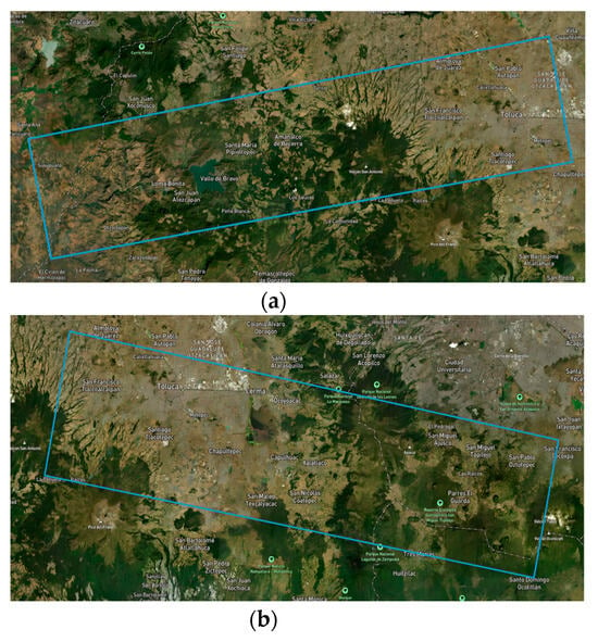
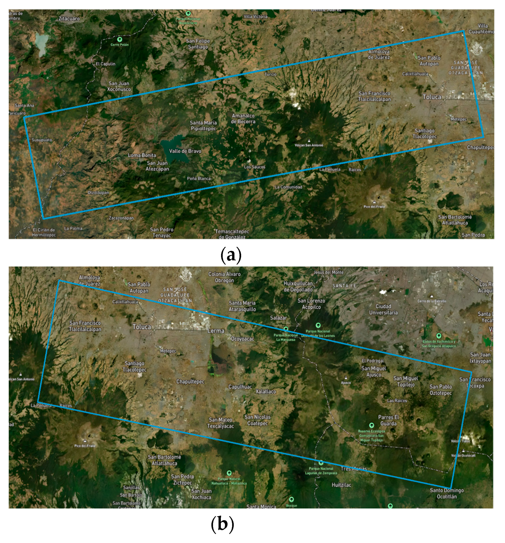
For the data processing phase, two specific bursts defined as individual segments of a Sentinel-1 image were selected to evaluate the geohazard susceptibility of the railway. The primary scene, illustrated in Figure 1a, was acquired utilizing the Interferometric Wide (IW) swath mode in an ascending geometry. This dataset corresponds to track 78, features Vertical-Vertical (VV) polarization, and belongs to absolute orbit 51950, specifically identified under the nomenclature 078_165500_IW2 with a Burst index of 6. Conversely, the secondary scene, depicted in Figure 1b, was captured in a descending orbit under the same IW mode and VV polarization. This specific dataset aligns with track 41, absolute orbit 52088, and is cataloged as 041_086879_IW1 with a Burst index of 2.

Figure 1. Area of land covered by satellite images: (a) ascending direction; (b) descending direction.

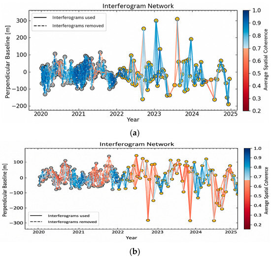
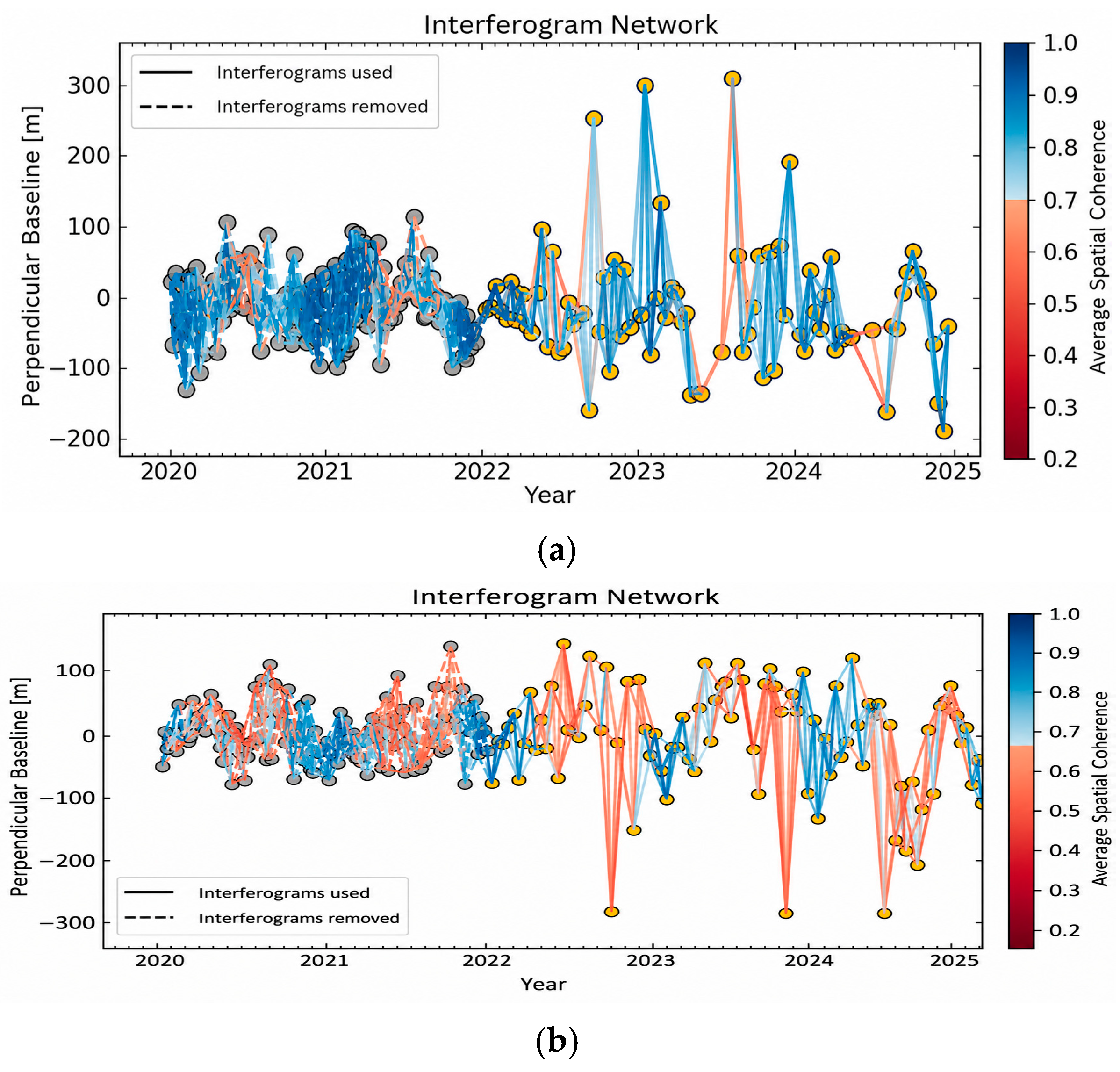
Based on these selected scenes, an extensive set of interferograms was computationally generated by cross-multiplying various image pairs. For the descending mode data, an initial network of 919 interferograms was created spanning from 2020 to late 2024, geometrically constrained by a maximum perpendicular baseline of 407.19 m and a temporal baseline of 96 days. Similarly, utilizing the ascending imagery, 920 interferograms were generated for the identical 2020–2024 timeframe, restricted by a maximum spatial baseline of 392.96 m and a temporal baseline of 36 days. The entirety of this initial interferometric formation was executed utilizing the Alaska Satellite Facility (ASF) Vertex platform, featuring the application of a 20 × 4 multilook filter to enhance signal quality [29]. This filtering configuration results in a pixel spacing of 80 m and an effective spatial resolution of 160 m. This pixel spacing establishes the fundamental horizontal baseline required for the subsequent geohazard susceptibility assessment, preventing sub-pixel resampling artifacts. However, to optimize the time-series inversion and focus exclusively on the most recent structural state of the railway corridor, the monitoring period was subsequently refined to span from January 2022 through December 2024. This temporal truncation is the main reason for the reduction in the total number of interferograms used in the final SBAS inversion (retaining 217 descending and 252 ascending interferograms). Within the retained 2022–2024 period, all interferograms meeting the temporal and spatial baseline constraints were utilized, as visually confirmed by the absence of discarded pairs (dashed lines) in the later portions of Figure 2. While this thorough threshold reduces the network redundancy to approximately three connections per acquisition date, it guarantees a fully connected interferometric network composed only of high-coherence pairs. This continuous temporal linkage provides sufficient redundancy for a reliable Singular Value Decomposition (SVD) within the MintPy software, preventing isolated data clusters while significantly reducing noise. Additionally, it is important to note regarding the spatial coverage that while the descending dataset encompasses the entire evaluated railway segment, the selected ascending burst covers only approximately 16 km of the alignment. Consequently, the extraction of the 2D vertical and horizontal deformation vectors is restricted to this 16 km overlapping area.

Figure 2. Interferogram network: (a) ascending direction; (b) descending direction.

3.2. Methods

3.2.1. SBAS InSAR

As defined by Li et al., (2022) [30] and Hussain et al., (2025) [31], the multi-temporal Short Baseline Subset framework originally introduced by Berardino et al., (2002) [6] is engineered to extract highly precise displacement rates from a meticulously constrained interferometric network. By limiting spatial and temporal baselines, this algorithm effectively mitigates decorrelation artifacts. Following the initial topographic phase removal, the unwrapped phase difference ($\Delta {\phi }_i$) for a specific highly coherent pixel between two image acquisitions ($t1$ and $t2$) is mathematically expressed as [30]:

$$\Delta {\phi }_i={\displaystyle \frac{4\pi }{\lambda }}\left(d_{t2}-d_{t1}\right)+\Delta {\phi }_{topo}+\Delta {\phi }_{noise}$$

(1)

Within this equation, the term ${\displaystyle \frac{4\pi }{\lambda }}\left(d_{t2}-d_{t1}\right)$ represents the actual ground displacement occurring within the respective temporal interval. The $\Delta {\phi }_{topo}$ parameter accounts for residual topographic artifacts stemming from DEM inaccuracies, while $\Delta {\phi }_{noise}$ integrates atmospheric delays alongside phase unwrapping errors. To compute the cumulative displacements derived from the $M$ generated interferograms, the algorithm constructs a linear system of equations defined as $AV=\Delta \phi$ [31]. In this matrix formulation, $A$ denotes the design matrix interlinking the interferometric pairs with their respective time intervals, and $V$ represents the unknown velocity vector to be resolved. The mathematical resolution of this system is achieved either through standard Least Squares optimization for fully connected interferometric subsets, or via Singular Value Decomposition (SVD) when dealing with disconnected network clusters [30].

The computational execution of this time-series inversion was conducted utilizing the open-source Miami INsar Time-series software in Python (MintPy) (version 1.6.3) [32]. Operating on the coregistered and unwrapped interferometric stacks, this processing pipeline ultimately derives the final Line-Of-Sight (LOS) displacement vectors [32]. The initial phase of the workflow allows for the strategic refinement of the interferometric network, enabling the exclusion of low-quality data pairs and the selection of an optimal reference pixel and date. Furthermore, phase unwrapping errors are systematically corrected, employing bridging algorithms effective over water bodies and phase closure techniques designed for highly redundant networks [32].

Following this pre-processing stage, the network is inverted using a weighted least squares approach to retrieve the phase time-series. A critical quality metric, the temporal coherence (${\gamma }_{temp}$), is subsequently computed for each pixel to quantify the goodness-of-fit between the mathematical model and the interferometric observations. To ensure reliability, only pixels satisfying a threshold ${\gamma }_{temp}\ge$ 0.7 are retained for further analysis [32].

To isolate the pure displacement signal, sequential corrections are applied to the dataset. These adjustments mitigate tropospheric delays (utilizing global atmospheric models or empirical phase-elevation relationships), phase gradients (which must be removed when the primary interest is ground subsidence), and DEM errors through perpendicular baseline correlation [32]. In the concluding phase, the integrity of the corrected dataset is evaluated based on the residual phase. This involves calculating the Root Mean Square (RMS) of the phase per acquisition and its corresponding mean absolute deviation to establish statistical limits. Data points exceeding these outlier thresholds are discarded. Ultimately, the semi-static displacement velocities are derived by fitting a best-fit linear regression model to the thoroughly refined time-series data [32].

To transition from a theoretical SBAS framework to the reproducible configuration implemented in this study, the time-series inversion in MintPy was executed with specific parameter choices. Initial topographic phase contributions were removed using the GLO-30 Copernicus (~30 m resolution) DEM, followed by a residual topographic error correction to mitigate local DEM inaccuracies. To mask heavily decorrelated areas, a spatial coherence threshold of 0.7 was applied. Atmospheric delays were actively mitigated utilizing the Python-based Atmospheric Phase Screen (PyAPS) module integrated with the ERA5 global climate model. Additionally, phase unwrapping anomalies were corrected by applying a phase-closure methodology. Notably, spatial phase deramping was deliberately bypassed. Given the spatial extent of the analyzed railway corridor, long-wavelength orbital errors are negligible; applying a deramping function at this scale introduces a risk of artificially filtering out the genuine regional subsidence signal of the Toluca Valley. Finally, the displacement time-series was spatially tied to a highly coherent, reference pixel strategically located outside the subsiding lacustrine clay basin (19.233° N, 99.646° W), with the first acquisition epoch (5 January 2022, for the descending track, and 14 January 2022, for the ascending track) manually enforced as the temporal reference date.

3.2.2. Validation of InSAR Results with GNSS

The validation of InSAR results is conducted through a comparison with GNSS measurements. This procedure involves assessing both the temporal behavior of the time series and the accumulated displacement. To ensure a reliable verification, it is essential that a GNSS station has operated continuously throughout the entire InSAR processing period and is located within the same geographic area. Due to the way SAR images are acquired, the displacements derived from InSAR are defined along the LOS direction. In contrast, displacements obtained from GNSS receivers are expressed in three components: east, north, and up (ENU). Therefore, it is necessary to transform the ENU components into the LOS direction [32]. This conversion of GNSS-derived displacements can be performed using the following equation [33]:

$$dLOS={-d}_{east}sin\left(\theta \right)cos\left(\alpha \right)+d_{north}sin\left(\theta \right)sin\left(\alpha \right)+d_{up}cos\left(\theta \right)$$

(2)

where $dLOS$ are the displacements in the LOS direction; $d_{east}, d_{north}, d_{up}$ are GNSS displacements in the east, north, and vertical directions, respectively; $\theta$ is the angle of incidence of the radar; $\alpha$ is the azimuthal angle.

Once the GNSS and InSAR data have been aligned in the same direction, they must be referenced to a common epoch. Subsequently, only the measurements that coincide in time between both techniques are then retained, while the remaining data are discarded. Validation involves calculating the following values: (1) coefficient of determination $\left(R^2\right)$ where a value close to 1 represents good temporal agreement; (2) Root Mean Square Error (RMSE), which serves as an indicator of the degree of difference between the measurements. For example, RMSE values ranging from 0.5 to 1.8 cm indicate a good level of agreement [32]; (3) Difference in accumulated displacement; (4) Difference between the velocities of displacement.

3.2.3. Geotechnical Hazard and Exposure Screening

Damage to urban infrastructure caused by subsidence is mainly attributable to the occurrence of ground displacements at varying rates. The angular distortion (β) is defined as the difference in vertical displacement between two adjacent points separated by a horizontal distance. In this study, the numerical thresholds used to classify the associated ground-level geotechnical hazard are adopted from the framework proposed by Cigna and Tapete (2021) [26]. To tailor this general scheme for a railway viaduct, the 1/500 upper bound is anchored with the AASHTO LRFD [34] bridge design specifications, acting as a safety factor of 2.0 relative to the 1/250 Service Limit State (SLS) for continuous-span structures. The 1/1500 and 1/3000 boundaries from the original scheme are retained as proposed graded screening levels with no codified structural meaning. Accordingly, the hazard risk is classified as follows:

•

Very high ($\beta >1/500$): For bridge design, the AASHTO LRFD [34] specifications recommend an angular distortion limit of ${\displaystyle \frac{\Delta }{L}}\le 0.004 \mathrm{r}\mathrm{a}\mathrm{d}$ (equivalent to 1/250) under the Service Limit State to prevent adverse secondary stresses, excessive cracking, and deck serviceability compromise in continuous-span structures. Therefore, adopting the upper geotechnical hazard threshold of $\beta$ = 1/500 (0.002 rad) introduces an inherent safety factor of 2.0 relative to the codified structural SLS limit. This conservative buffer accounts for the macro-scale resolution of InSAR data and acts as an early-warning screening criterion, capturing ground kinematic differentials capable of mobilizing asymmetric downdrag on pile groups well before structural capacity or superstructure serviceability is exhausted.

•

High ($1/1500<\beta \le 1/500$): Indicates a progressive acceleration of differential ground settlement trends. Geotechnically, this signifies a transition zone where asymmetric ground displacement actively begins to accumulate shear stresses in the soil surrounding the deep foundations. While still safely below the structural early-warning limits of the bridge, the terrain in this category exhibits sufficient distortion to initiate localized negative skin friction (downdrag), warranting prioritized geotechnical inspection of the pile cap environments.

•

Medium ($1/3000<\beta \le 1/1500$): Represents the onset of mild differential ground movement. Rather than indicating structural risk, this zone serves as a baseline geotechnical monitoring threshold. It reflects an incipient deviation from the uniform settlement profile, signaling areas where the terrain begins to experience localized gradients that could eventually develop uneven soil-structure interactions over time.

•

Low ($\beta \le 1/3000$): Defines a highly uniform regional settlement profile exhibiting rigid-body kinematic behavior. While widespread subsidence may still induce symmetric axial downdrag, the near-zero angular distortion minimizes differential shear stresses in the subsoil. This ensures the total absence of asymmetric downdrag, preventing the transfer of unwanted bending moments to the viaduct’s substructure.

These thresholds characterize differential ground settlement and surface deformation gradients, serving strictly as a conservative geotechnical screening tool. They do not represent the structural serviceability limits or ductility capacity of the pile-supported viaduct, which would require detailed structural design plans, mechanical material properties, and load test data to be formally established. Furthermore, while the spatial baseline of 160 m naturally exceeds the typical pier spacing of the viaduct (approximately 30 to 40 m), the proposed metric functions as a macro-scale corridor screening tool rather than a span-by-span structural SLS check.

3.2.4. Vertical and East–West Displacement Decomposition

To resolve the two-dimensional displacement fields, the LOS measurements from the ascending and descending geometries were combined. Due to the near-polar orbital trajectory of the Sentinel-1 satellites, the measurement sensitivity along the north–south direction is negligible; therefore, the horizontal north–south component was assumed to be zero ($d_N$ ≈ 0). Under this assumption, the relationship between the observed LOS displacements ($d_{LOS}^{asc}$) ($d_{LOS}^{des}$), the vertical ($d_V$) and east–west ($d_h$) displacement components are governed by the following linear system [35]:

$$\left[d_{LOS}^{asc} d_{LOS}^{des}\right]=\left[cos{\theta }_{asc}-{sin\theta }_{asc}{cos\alpha }_{asc}{cos\theta }_{des}-{sin\theta }_{des}{cos\alpha }_{des}\right] \left[d_v{d}_h\right]$$

(3)

where $\theta$ and $\alpha$ represent the local radar incidence angle and satellite heading angle, respectively. Prior to the mathematical decomposition, the spatial alignment of both ascending and descending geometries was executed within the MintPy framework.

Rather than directly resampling one radar geometry onto the other, both datasets were independently projected from their native radar coordinates (azimuth/range) onto a predefined geographic grid (EPSG:32614) utilizing DEM-derived lookup tables. The line-of-sight velocity fields were resampled to a common spatial resolution using nearest-neighbor interpolation. Finally, these harmonized grids were integrated within a unified spatial framework to analytically solve the vertical and horizontal deformation vectors.

4. Results

4.1. Validation

To strictly verify the reliability of the InSAR-derived displacements, geodetic measurements were acquired from the Nevada Geodetic Laboratory (NGL) at the University of Nevada, Reno. Operating as a GNSS data processing center, the NGL guarantees positional accuracy by employing the GipsyX software alongside highly precise orbit and clock products provided by the National Aeronautics and Space Administration (NASA) [36]. The ground truth data for this assessment were exclusively sourced from the MXTO continuous reference station situated in Toluca. The fundamental geographical and operational parameters of this specific station are detailed in Table 2 [37].

Table 2. GNSS Station Features [37].

Characteristics	Specifications
Station ID	MXTO
Latitude	19.280 degrees
Longitude	−99.608 degrees
Height	2634.078 m

Prior to quantitative validation, the relative InSAR displacements were temporally aligned with the MXTO GNSS station. The spatial reference pixel for the InSAR processing was established at 19.233° N, 99.646° W, a location selected outside the subsiding lacustrine clay basin. Although this reference point is situated 6.5 km away from the GNSS antenna, anchoring the phase inversion to this geological datum ensures that the measured displacements reflect true regional geodetic trends rather than localized phase unwrapping errors. Temporally, both datasets were initialized to zero at the first acquisition epoch (5 January 2022, for the descending track, and 14 January 2022, for the ascending track), enabling a direct comparison of cumulative displacements across the 152 coincident satellite-GNSS epochs.

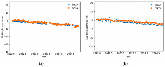
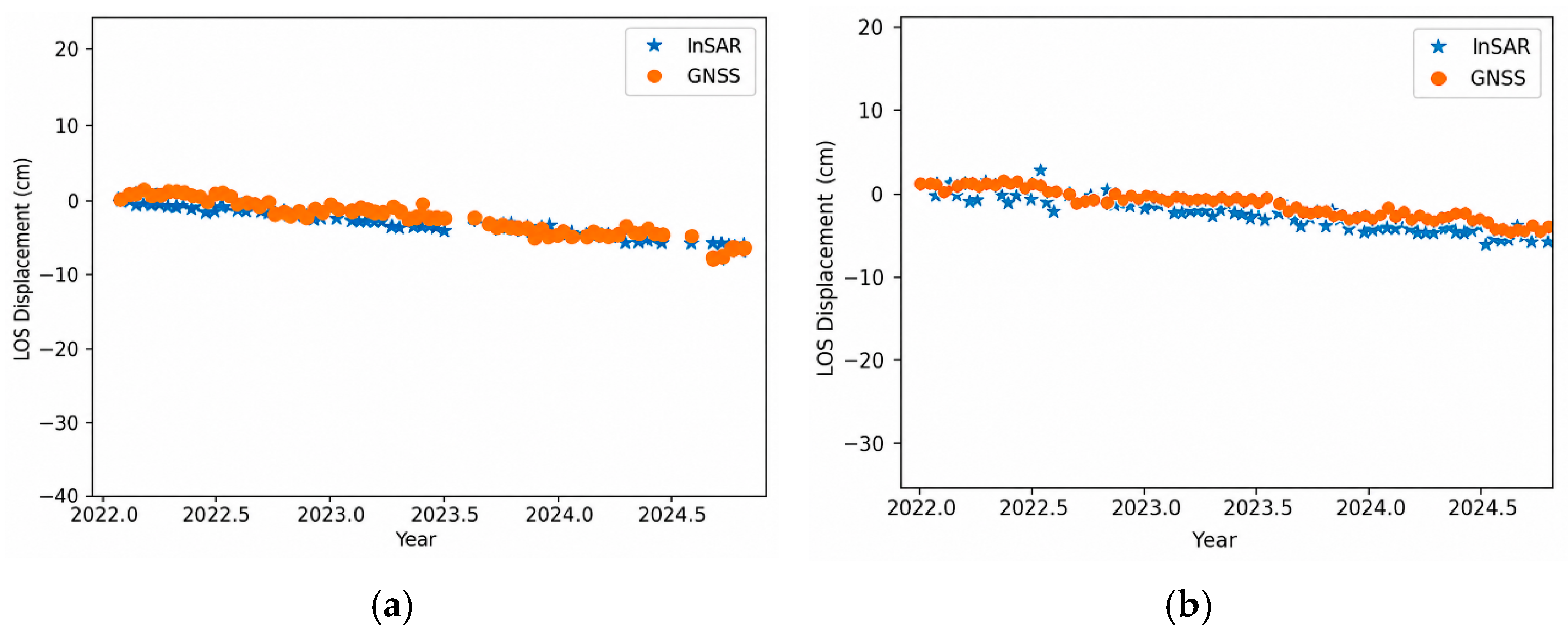
A quantitative comparison between the InSAR-based estimates and the ground truth GNSS data revealed an agreement across both orbital configurations. For the descending trajectory, the LOS displacement measurements yielded an RMSE of 1.09 cm, alongside a cumulative displacement disparity of −0.373 cm and a velocity difference of −0.6 cm/year. Additionally, this geometry achieved a temporal coherence of 0.99, and a coefficient of determination (R²) of 0.86. Similarly, the ascending path analysis produced an RMSE of 1.41 cm, a cumulative displacement offset of 1.63 cm, and a velocity difference of 0.35 cm/year, while maintaining a high temporal coherence of 0.97, and an R² of 0.80.

These computed statistical metrics confirm the successful execution of the InSAR processing, as they comfortably achieve the established quality thresholds in remote sensing literature. Contemporary studies advocate for an R² ≥ 0.7 [38], a displacement RMSE ≤ 1.8 cm [32], a vertical velocity RMSE ≤ 13 mm/year [39], and a temporal coherence ≥ 0.7 [32]. The chronological evolution of these highly correlated displacement trends can be visually analyzed in the time-series comparison presented in Figure 3.

Figure 3. Comparison of InSAR results with respect to the MXTO GNSS station: (a) ascending direction; (b) descending direction.

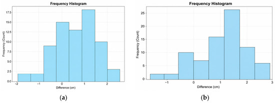
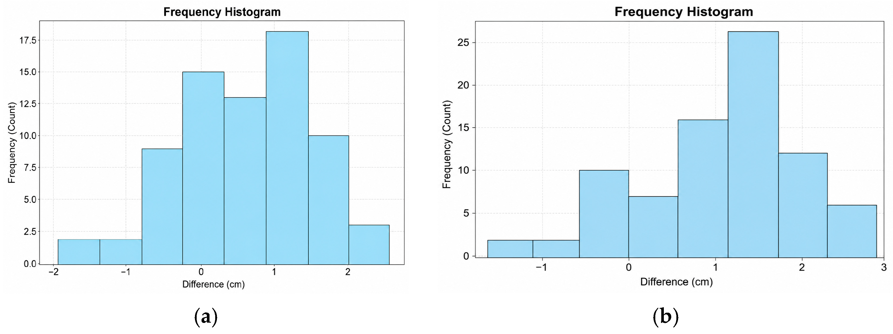
Further statistical scrutiny of the differences between the InSAR outputs and the GNSS records highlighted the stability of the multitemporal inversion. In the descending mode, the recorded systematic datum offset exhibited a mean of 0.59 cm and a standard deviation of 0.91 cm, fluctuating between a minimum of −1.94 cm and a maximum of 2.56 cm. Similarly, the ascending mode discrepancies demonstrated a mean value of 1.08 cm with a standard deviation of 0.89 cm, encompassing a range from −1.55 cm to 2.80 cm. The statistical distribution of these residuals is graphically represented in the histogram in Figure 4. It is important to note that these non-zero-centered distributions do not merely represent random phase variance or atmospheric noise, but rather indicate a systematic datum offset. InSAR measurements are inherently relative to a designated reference pixel, whereas the MXTO GNSS station provides absolute displacement measurements within a global reference frame. Given the regional subsidence dynamics of the Toluca Valley, any spatial separation and consequent differential subsidence between the InSAR reference point and the physical location of the GNSS antenna introduces a constant shift in the relative InSAR time-series. Therefore, these near-centimeter positive biases accurately reflect this systematic datum offset between the absolute GNSS reference frame and the relative InSAR network, validating the overall trend of the measurements.

Figure 4. Histogram of the differences between InSAR measurements and GNSS observations: (a) descending orbit; (b) ascending orbit.

Although validating a regional transport corridor extending several tens of kilometers ideally benefits from multiple spatially distributed geodetic points, the availability of public, continuously operating geodetic GNSS stations in the Toluca Valley is highly constrained. During the analyzed 2022–2024 period, the MXTO station operated by the Nevada Geodetic Laboratory was the only active and reliable continuous geodetic reference available in the immediate vicinity of the corridor. Validating wide-area railway InSAR results with a single available continuous GNSS station is a well-established precedent in peer-reviewed literature under similar regional data constraints. For instance, Shami et al. (2022) [4] monitored land subsidence and stability along the 110-km-long Qom–Kashan railway in Iran using Sentinel-1 data, validating their multi-temporal InSAR results against only a single permanent GNSS receiver (Aran station) due to the lack of wider instrumentation. To maximize accuracy under this constraint, the time series was validated on a highly coherent reference pixel adjacent to the geodetic station across 152 temporally coincident epochs, confirming the stability of the interferometric dataset.

4.2. Descending and Ascending Direction

To characterize the magnitude and spatial distribution of ground displacement, quantitative LOS measurements from both descending and ascending orbital configurations were subjected to comprehensive descriptive statistical analysis.

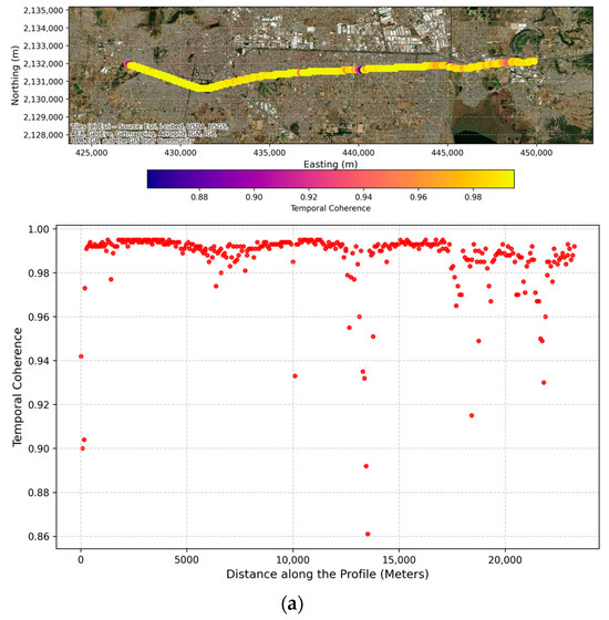
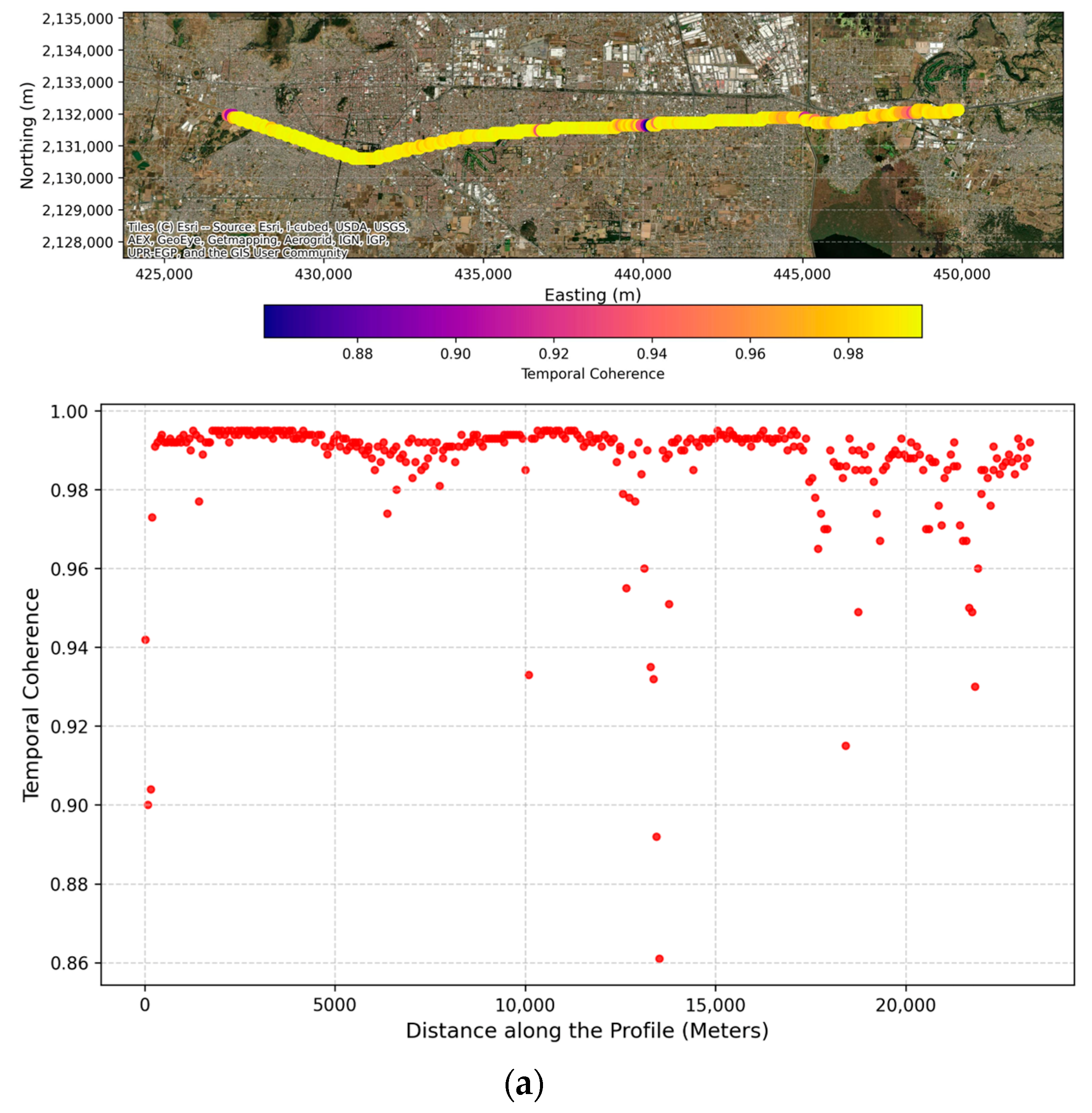
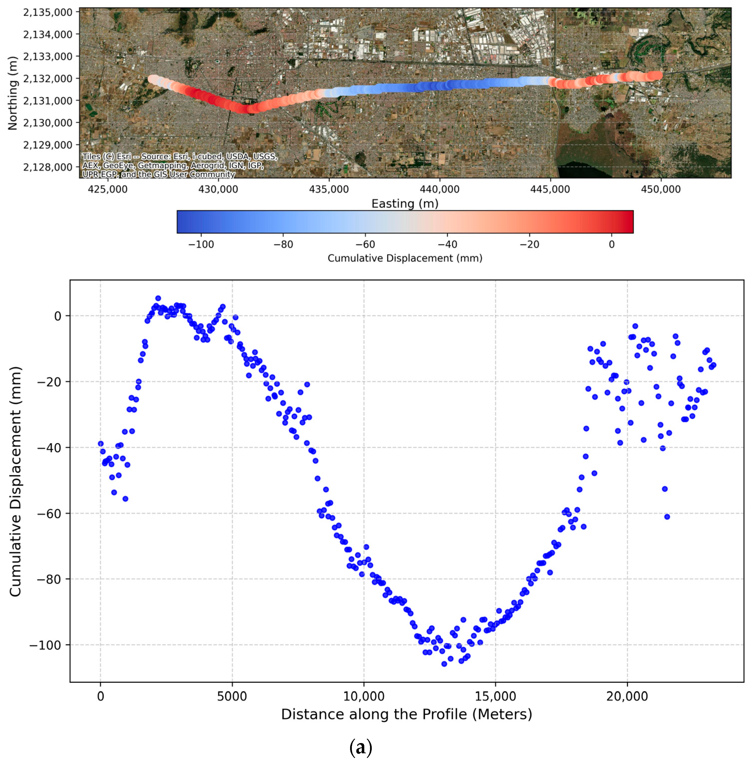
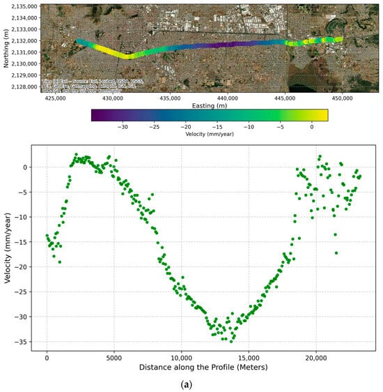
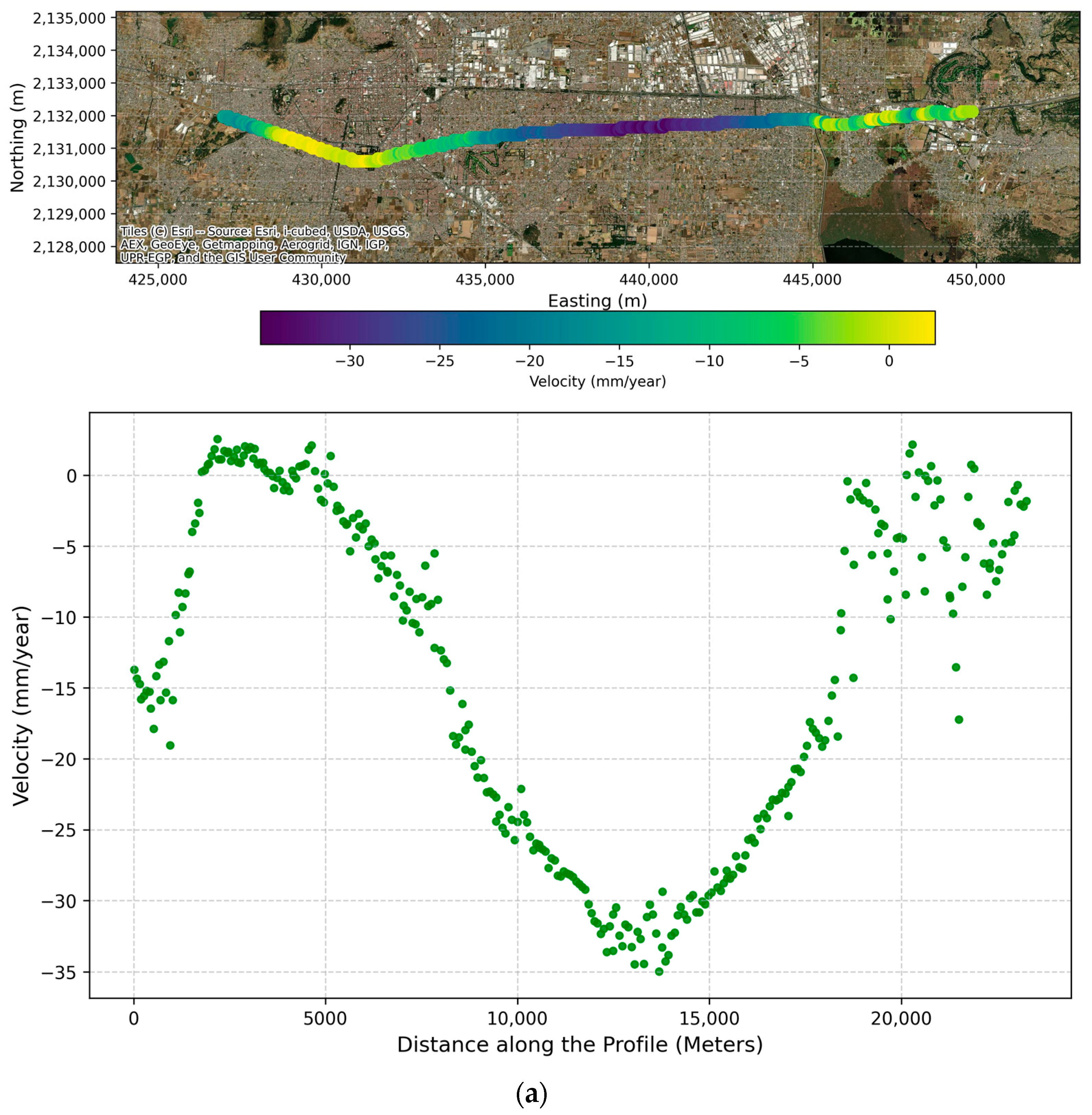
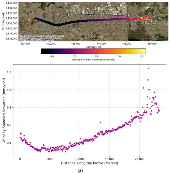
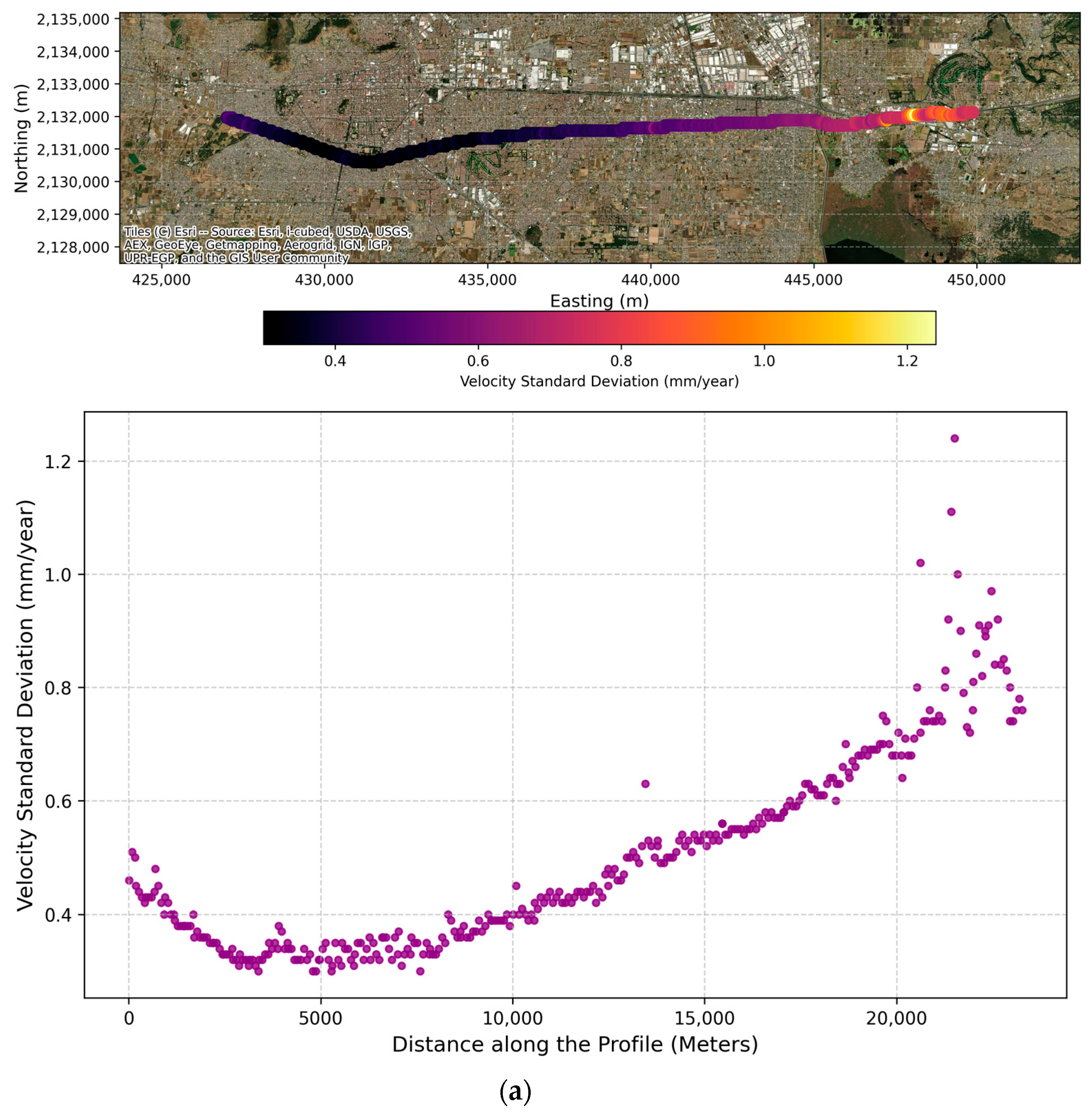
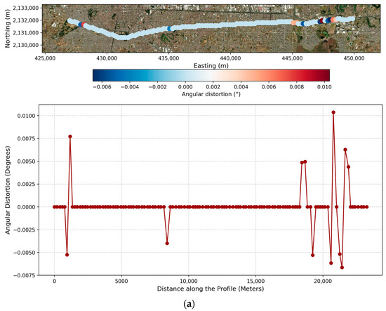
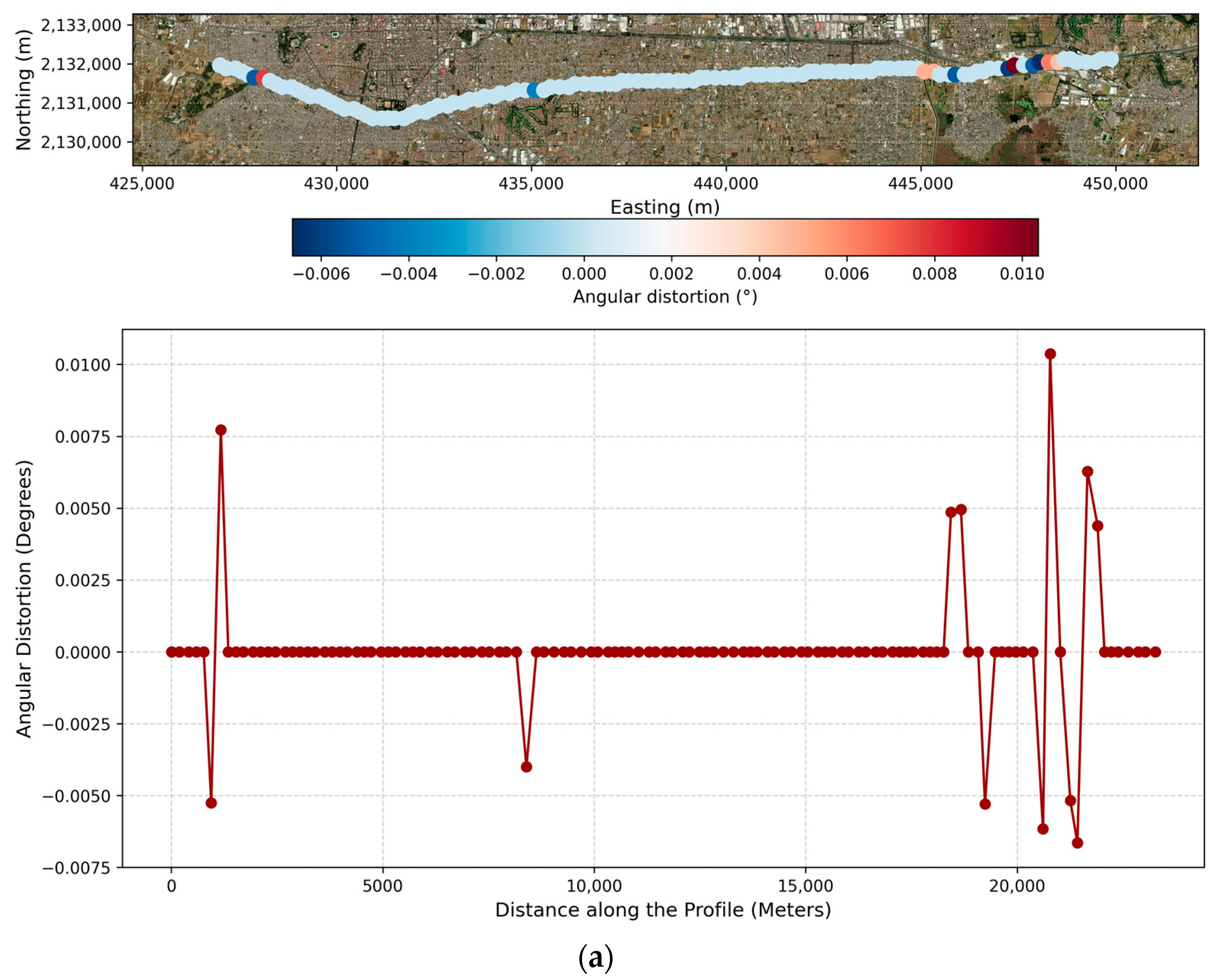
For the descending trajectory, the interferometric network demonstrated high stability, exhibiting a mean temporal coherence of 0.98. The corridor displays an active subsidence regime, with a mean LOS velocity of −13.4 mm/year and localized maximum subsidence rates reaching −34.9 mm/year. The central tendencies, dispersion parameters, and extreme boundaries for these measurements are consolidated in Table 3, encompassing temporal coherence (Figure 5a), primary kinematic outputs—cumulative displacements, velocities, and associated standard deviations (Figure 6a, Figure 7a and Figure 8a)—and unilateral angular distortion (Figure 9a). Specifically, the descending angular distortion yielded a mean of 0.00005° (standard deviation = 0.0019°), fluctuating between −0.0066° and 0.0103°.

Table 3. Statistical Summary of the Results for the Descending Track.

Variable	Mean	Standard Deviation	Minimum	Maximum	Figure
Temporal Coherence	0.98	0.02	0.86	0.99	Figure 5a
Accumulated Displacement	−44.6 mm	34.8 mm	−105.8 mm	5.3 mm	Figure 6a
Velocity	−13.4 mm/year	11.8 mm/year	−34.9 mm/year	2.6 mm/year	Figure 7a
Standard Deviation of Velocity	0.5 mm/year	0.2 mm/year	0.3 mm/year	1.2 mm/year	Figure 8a
Angular Distortion	0.00005°	0.0019°	−0.0066°	0.0103°	Figure 9a

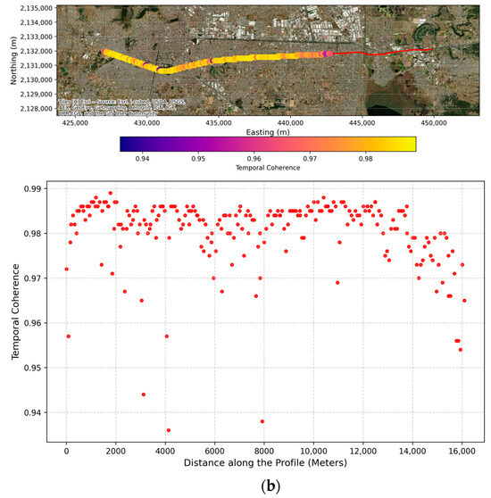
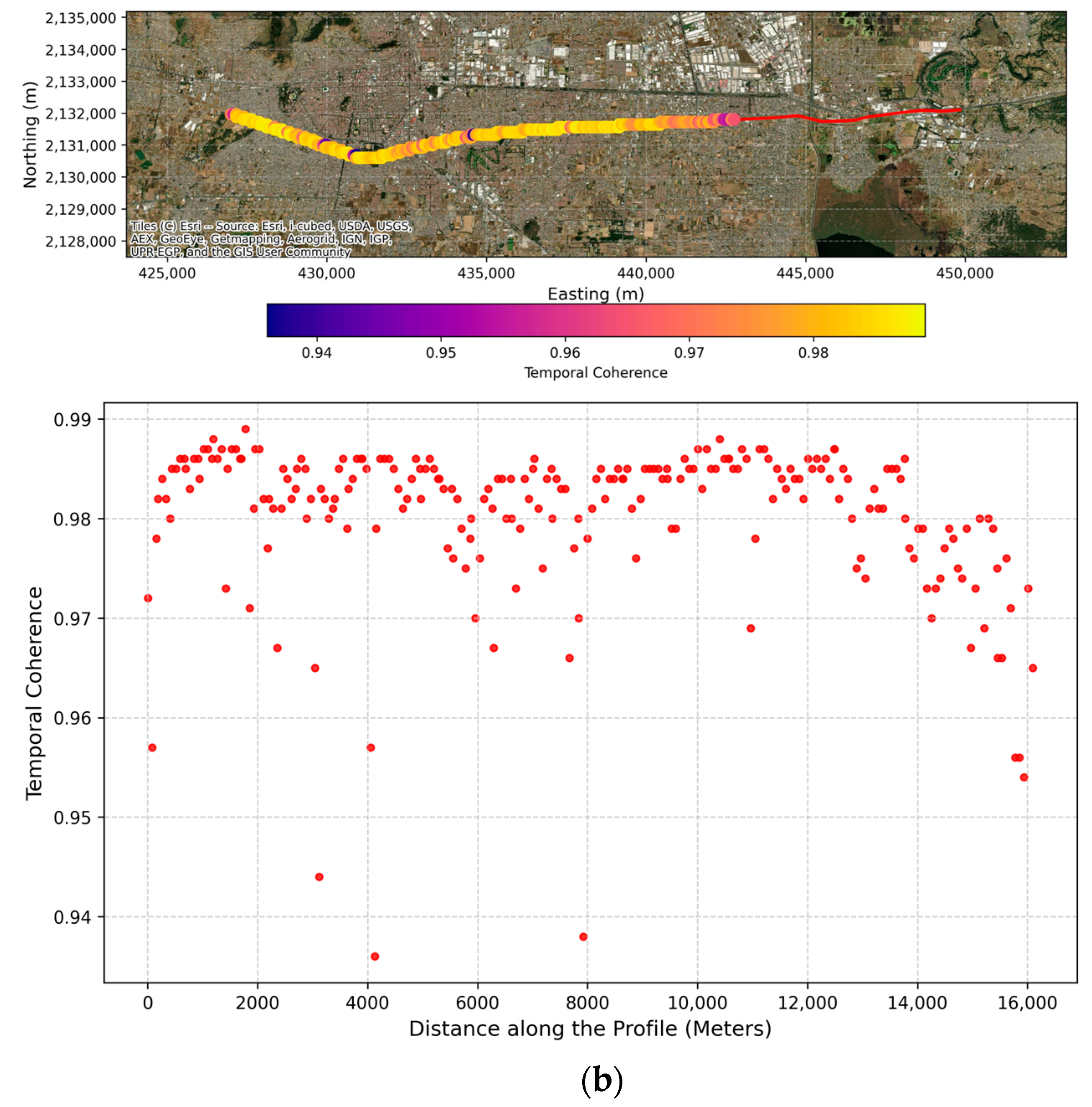
Figure 5. Temporal coherence from InSAR processing for (a) the descending-track and (b) the ascending-track.

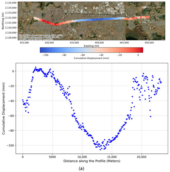
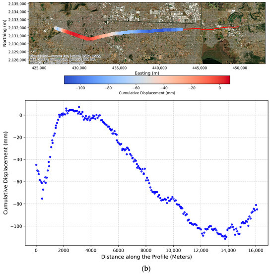
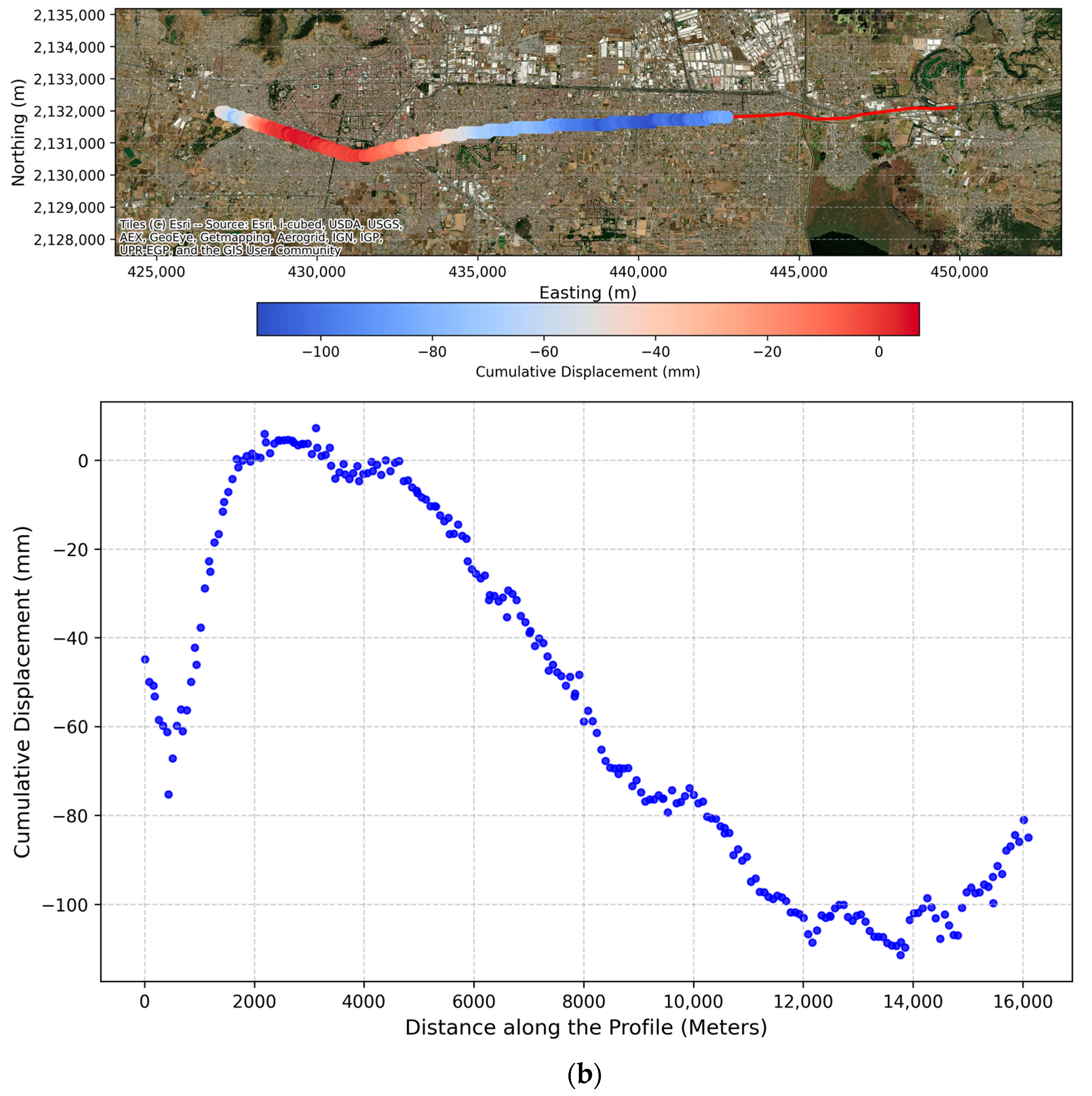
Figure 6. Cumulative displacement resulting from InSAR processing for (a) the descending-track and (b) the ascending-track.

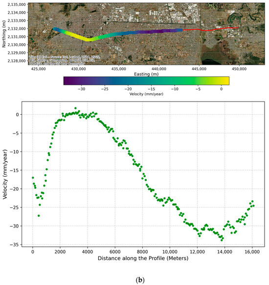
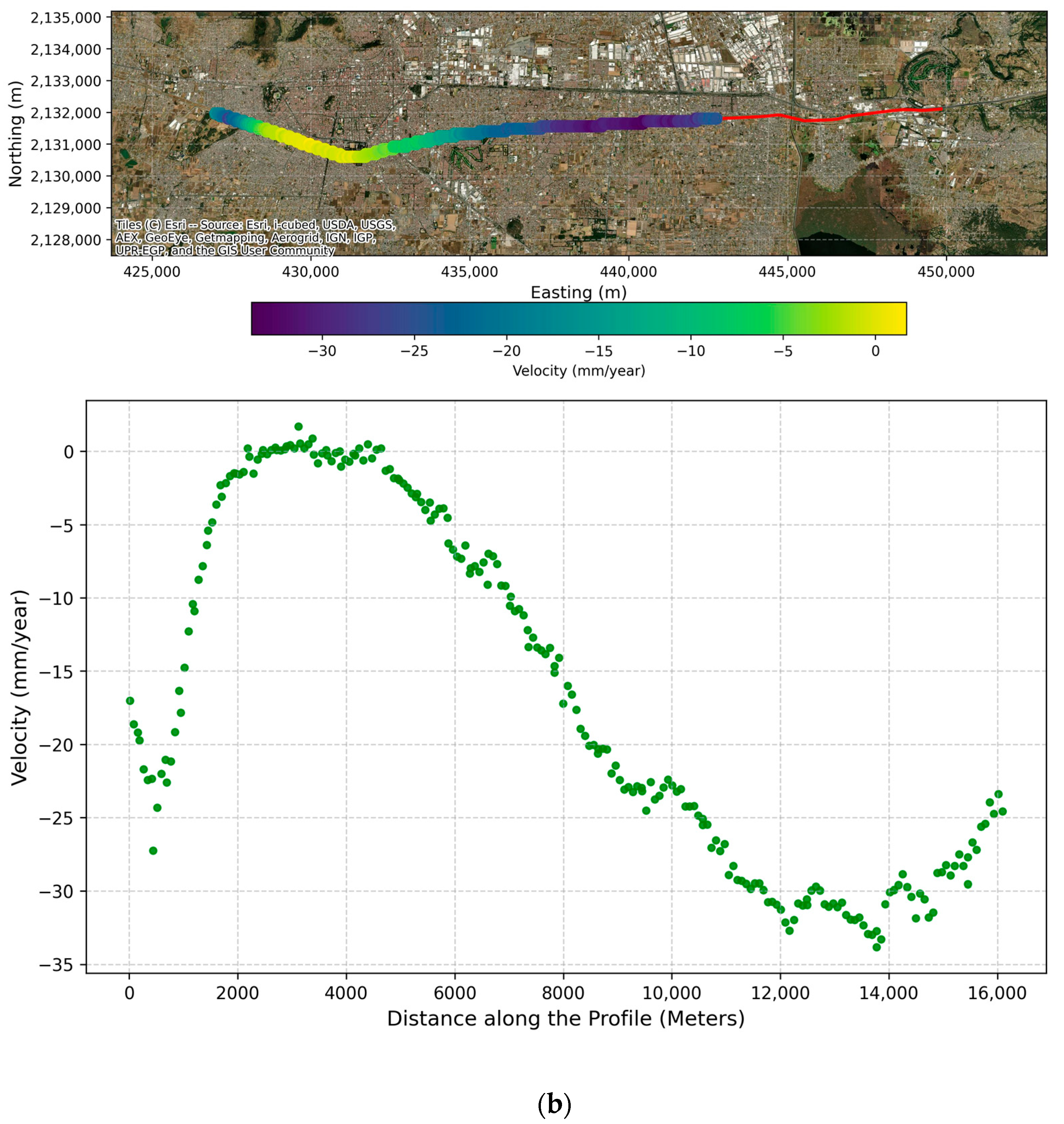
Figure 7. Velocity derived from InSAR processing for (a) the descending-track and (b) the ascending-track.

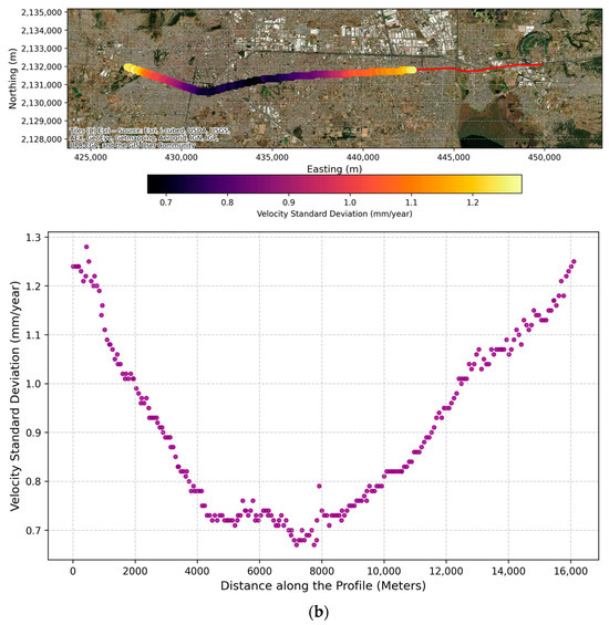
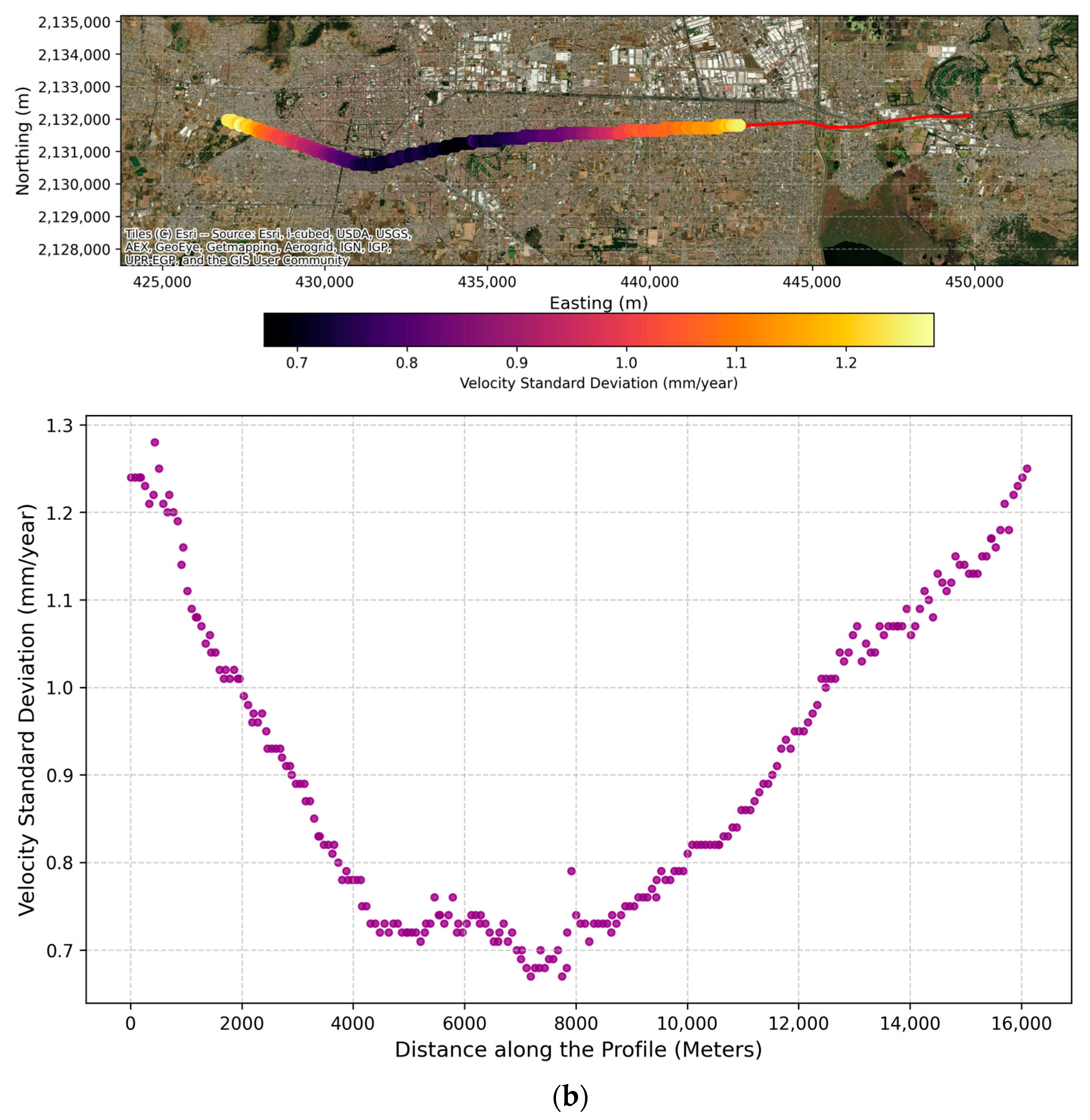
Figure 8. Standard deviation of the velocity derived from InSAR processing for (a) the descending-track and (b) the ascending-track.

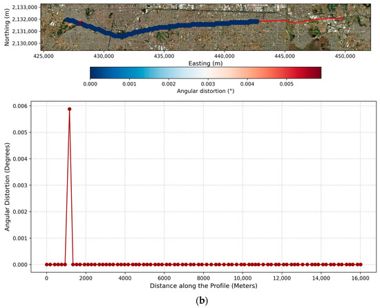
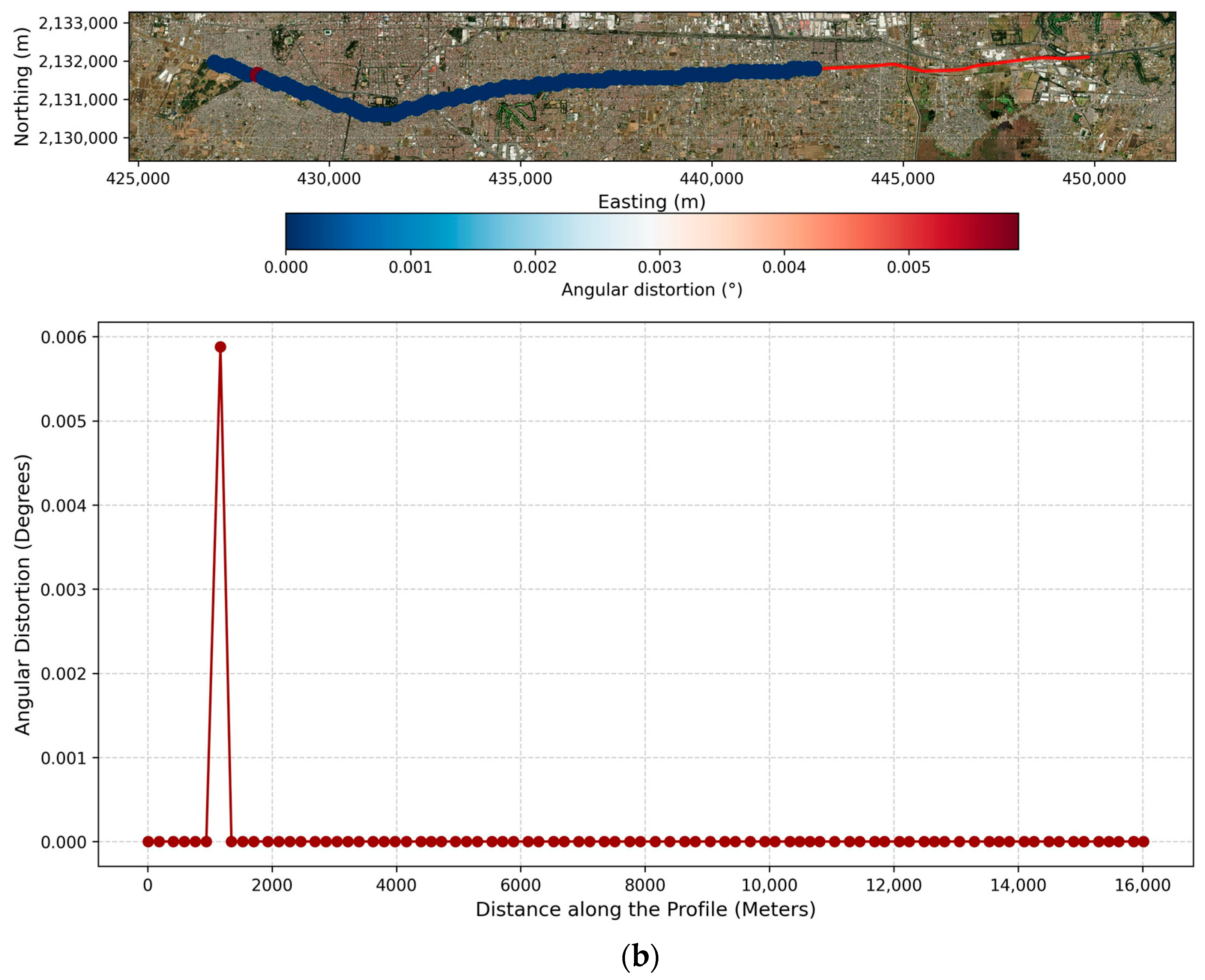
Figure 9. Angular distortion along the Mexico-Toluca Interurban Train corridor derived from InSAR processing results for (a) the descending track and (b) the ascending track.

Similarly, the ascending track analysis revealed an active displacement trend with a mean LOS velocity of −16.2 mm/year, cumulative displacements reaching −111.4 mm, and a mean temporal coherence of 0.98. The corresponding statistical metrics are summarized in Table 4 and illustrated across Figure 5b to Figure 9b, where the ascending angular distortion recorded a mean of 0.000072° (SD = 0.000649°), ranging from 0.00° to 0.005879°. When evaluating these magnitudes, the intrinsic uncertainty of the InSAR measurements was explicitly considered. Consequently, any localized extreme values that fell within this error margin were discarded. Furthermore, the discrepancies in the calculated angular distortion between the ascending and descending datasets stem from the inherent geometric limitations of unilateral LOS gradients. Because angular distortion is derived from the spatial gradient of differential displacement, single-geometry LOS calculations are sensitive to the sensor’s specific incidence and heading angles. Any horizontal ground motion projects unevenly into the ascending and descending LOS vectors, artificially skewing the apparent differential displacement and yielding conflicting angular distortion values for the same physical location.

Table 4. Statistical Summary of the Results for the Ascending Track.

Variable	Mean	Standard Deviation	Minimum	Maximum	Figure
Temporal Coherence	0.98	0.008	0.93	0.989	Figure 5b
Accumulated Displacement	−53.1 mm	40.1 mm	−111.4 mm	7.3 mm	Figure 6b
Velocity	−16.2 mm/year	11.9 mm/year	−33.8 mm/year	1.7 mm/year	Figure 7b
Standard Deviation of Velocity	0.9 mm/year	0.2 mm/year	0.7 mm/year	1.3 mm/year	Figure 8b
Angular Distortion	0.000072°	0.000649°	0.00°	0.005879°	Figure 9b

To establish a robust quantitative baseline for geohazard susceptibility along the Mexico-Toluca Intercity Railway corridor, Table 5 and Table 6 present a synthesis of the calculated vertical subsidence velocities and their associated standard deviations. These metrics are designed to serve as foundational geotechnical reference parameters for future monitoring frameworks. By utilizing these values, engineers can implement statistical control limits—specifically, defining anomaly thresholds at the mean velocity $\pm 3$ standard deviations—to proactively detect any future kinematic deviations from the current regional subsidence trend. The baseline velocities represent single-pixel values sampled at discrete 1-km intervals to establish macroscopic, easily locatable control points.

Table 5. Summary of Velocity and Its Standard Deviation (Descending Track).

Control Point Index	Location in Profile (m)	Velocity (mm/Year)	Standard Deviation of Velocity mm/Year
1	1019.41	−15.86	0.42
2	2031.50	1.37	0.36
3	3043.37	2	0.32
4	4055.17	−1.08	0.34
5	5049.57	−0.54	0.34
6	6038.98	−3.37	0.35
7	7011.42	−10.25	0.33
8	8079.32	−12.98	0.34
9	9042.60	−20.09	0.37
10	10,005.77	−24.46	0.40
11	11,048.96	−28.22	0.42
12	12,007.76	−31.41	0.44
13	13,050.76	−34.46	0.50
14	14,013.65	−32.43	0.50
15	15,053.01	−29.41	0.52
16	16,015.74	−25.71	0.54
17	17,054.18	−21.97	0.58
18	18,018.50	−18.7	0.61
19	19,080.00	−0.52	0.68
20	20,042.27	−4.46	0.72
21	21,018.27	−1.69	0.74
22	22,065.98	−3.55	0.86
23	23,031.34	−0.67	0.74

Table 6. Summary of velocity and its standard deviation (ascending direction).

Control Point Index	Location in Profile (m)	Velocity (mm/Year)	Standard Deviation of Velocity (mm/Year)
1	1019.41	−14.75	1.11
2	2031.50	−1.57	0.99
3	3043.37	0.2	0.89
4	4055.17	−0.69	0.78
5	5049.57	−2.19	0.72
6	6038.98	−7.18	0.73
7	7011.42	−10.53	0.69
8	8079.32	−16.01	0.73
9	9042.60	−22.43	0.75
10	10,005.77	−22.81	0.81
11	11,048.96	−28.91	0.86
12	12,007.76	−31.25	0.95
13	13,050.76	−31.08	1.07
14	14,013.65	−30.08	1.06
15	15,053.01	−28.23	1.13
16	16,015.74	−23.39	1.24

4.3. Vertical and Horizontal Velocity

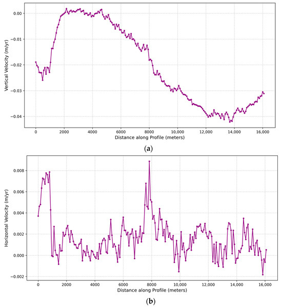
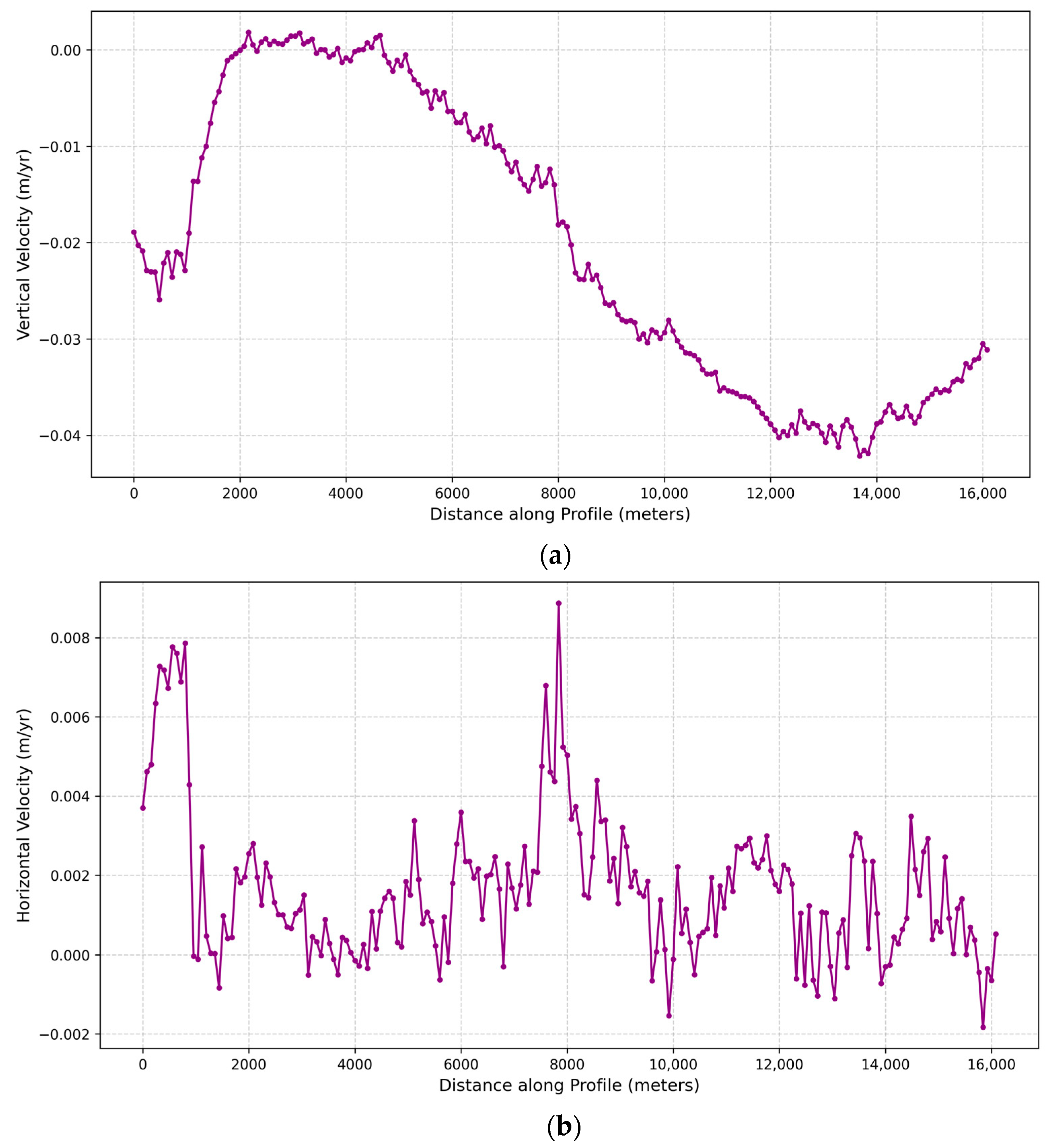
Inherently, standard InSAR processing yields one-dimensional displacement measurements projected along the satellite’s Line-Of-Sight. However, comprehensively characterizing the true behavior of the railway infrastructure requires decomposing these singular vectors into their actual vertical and horizontal (east–west) components. This geometric decomposition mandates the spatial intersection of both the ascending and descending datasets. Consequently, the derived two-dimensional velocity profiles are restricted to the overlapping swath of the employed image bursts, spanning an approximate 16-km corridor originating from the Zinacantepec terminal. This specific analytical segment encompasses critical transit nodes, including the Zinacantepec (≈0 km), Pino Suarez (≈5.8 km), and Tecnológico (≈12.9 km) stations. The spatial distribution of the computed vertical and horizontal velocities across this railway section is visually depicted in Figure 10.

Figure 10. Velocity derived from InSAR processing: (a) Vertical; (b) Horizontal.

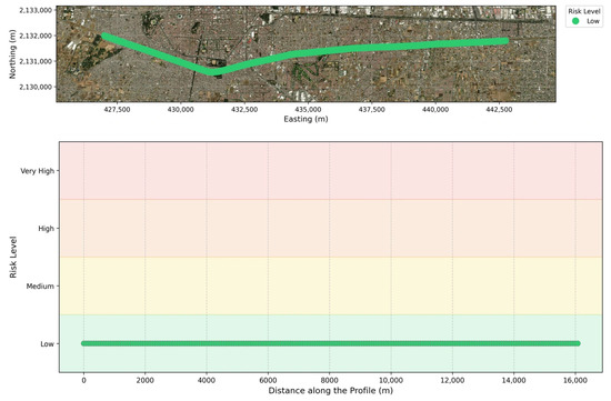
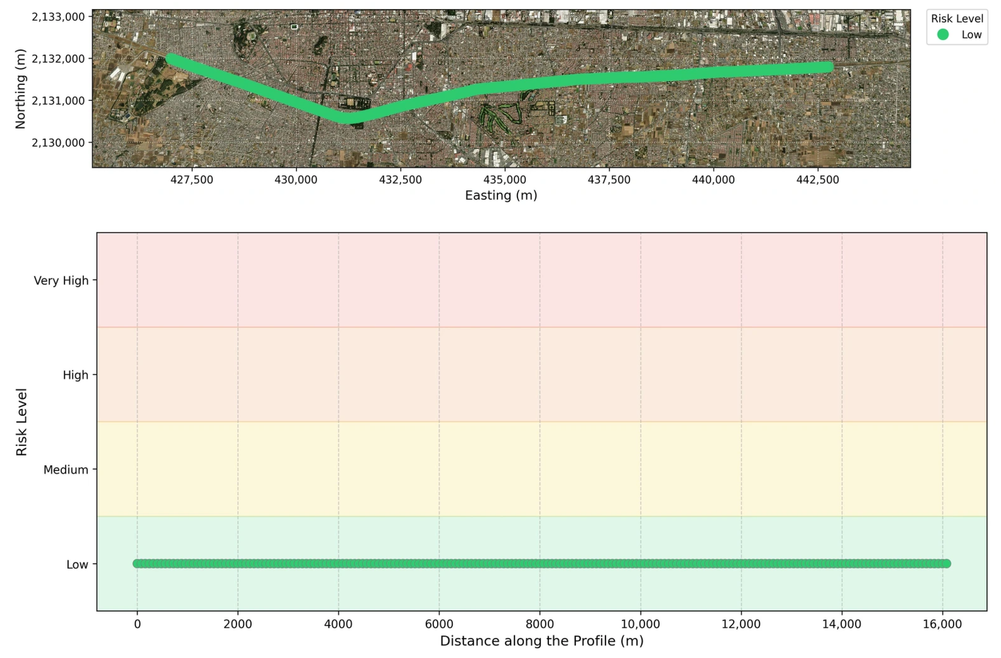
A statistical evaluation of the decomposed vectors highlights the predominance of vertical settlements over lateral movements. The vertical velocity field exhibited a mean subsidence rate of −2 cm/year, accompanied by a standard deviation of 1.5 cm/year, reaching a maximum localized settlement of −4.2 cm/year and a peak positive variation of 2 mm/year. Conversely, the horizontal velocity profile proved to be marginal, presenting a mean eastern displacement of 2 mm/year and a standard deviation of 2 mm/year. The horizontal boundaries fluctuated between −2 mm/year (indicative of westward movement) and a maximum of 9 mm/year towards the east. Building upon these kinematic results, the isolated vertical displacement provides the definitive physical metric for assessing the differential ground settlement directly impacting the infrastructure. Therefore, a refined assessment was conducted exclusively utilizing this vertical component within the 16-km overlapping zone. To evaluate the geohazard susceptibility of the Mexico-Toluca Intercity Railway while preventing sub-pixel resampling artifacts, the overlapping segment was sampled at 160-m horizontal intervals, yielding a total of 200 point pairs along the alignment. The statistical analysis of the raw, unfiltered vertical displacement differences between these adjacent locations revealed an absolute mean difference of just 1.3 mm, with a standard deviation of 1.2 mm. Crucially, the maximum vertical differential detected across any 160-m span was 9.3 mm. Because this maximum recorded value falls entirely within the GNSS-validated root mean square error (RMSE) margin of the InSAR measurements, all detected vertical variations are statistically indistinguishable from the inherent phase noise of the SAR signal. Consequently, these millimeter-level differences reflect the uncertainty of the measurement rather than true differential ground motion. Even when conservatively applying these unfiltered, noise-driven values to compute the ground distortion gradient, the maximum resulting ratio is approximately 1/17,204. As illustrated in the resulting susceptibility profile (Figure 11), this positions the entire evaluated railway segment uniformly and within the low-risk category (<1/3000). This continuous stability confirms that the regional land subsidence (the primary geohazard) affects the terrain beneath the viaduct homogeneously, inducing no significant differential ground settlements that could transfer damaging stresses to the railway infrastructure.

Figure 11. Risk level along the Mexico-Toluca Interurban Train profile derived from vertical InSAR processing results.

To ensure that the geohazard classification is not an artifact of the chosen sampling interval, a baseline sensitivity analysis was conducted utilizing a continuous rolling window approach. The maximum vertical differential was evaluated across multiple spatial baselines (80 m, 160 m, and 320 m) and compared against the intrinsic InSAR measurement uncertainty. As demonstrated in Table 7, the maximum vertical differentials detected at all three spatial scales (5.3 mm, 9.3 mm, and 11.7 mm, respectively) remain securely within the uncertainty margin, confirming that the low-risk classification is physically invariant to the sampling interval. However, it is essential to consider that the multilooking applied during the InSAR processing pipeline acts as a spatial low-pass filter. While this spatial averaging strengthens the regional assessment, it naturally smooths and attenuates highly localized, high-frequency deformation gradients, further underscoring the metric’s designated role as a macro-scale corridor screening tool.

Table 7. Baseline sensitivity analysis of vertical differentials along the 16-km evaluated segment.

Spatial Baseline (m)	Mean (mm)	Standard Deviation (mm)	Minimum (mm)	Maximum (mm)
80	0.92	0.81	0	5.3
160	1.3	1.2	0.01	9.3
320	1.9	1.8	0.01	11.7

4.4. Visual Inspection

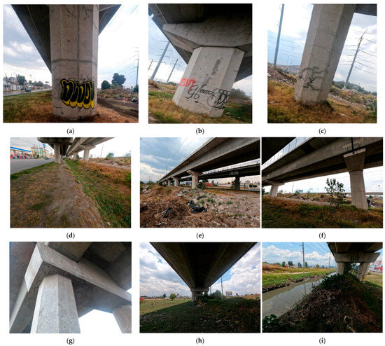
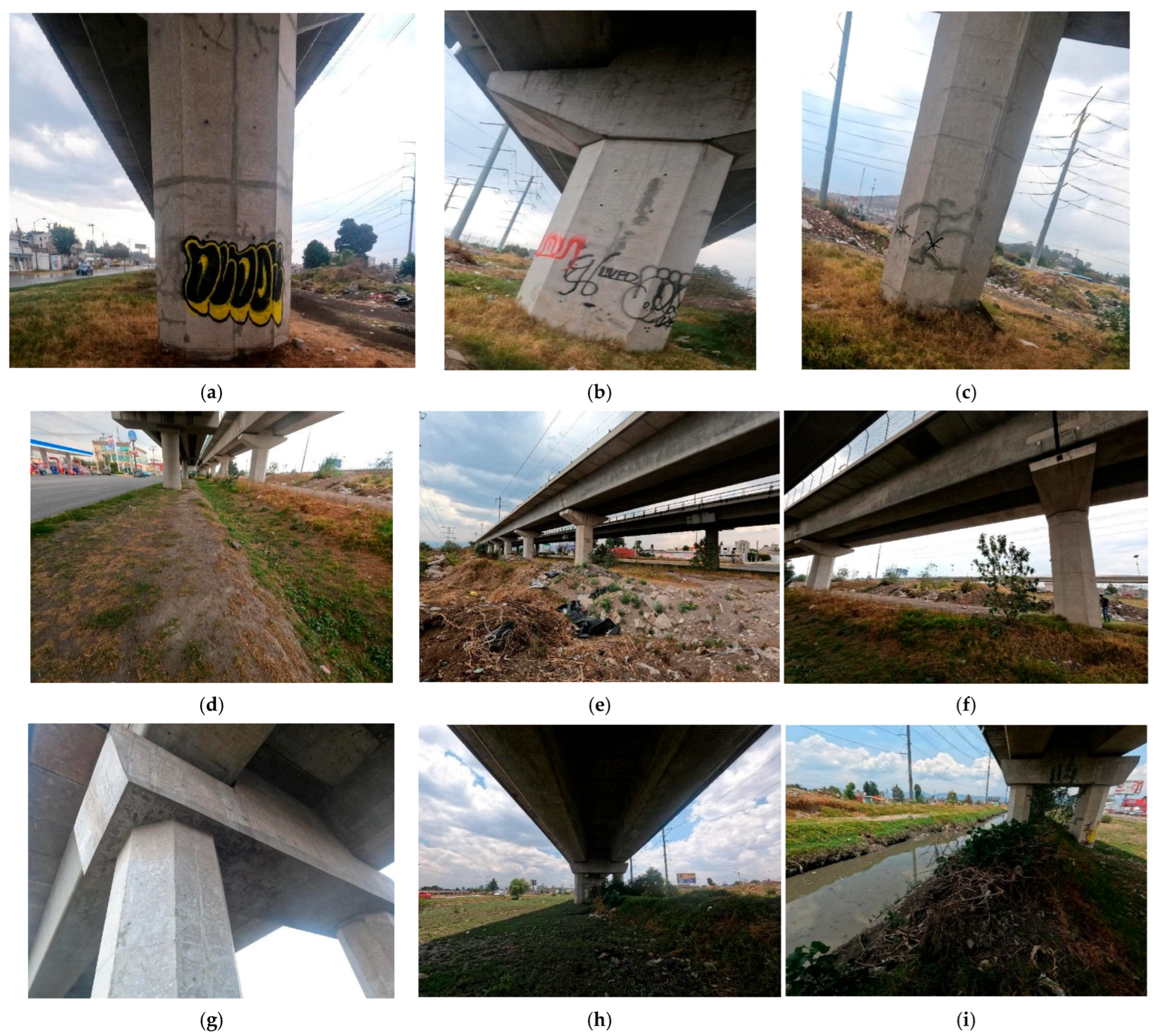
To validate the physical significance of the deformation gradients flagged by the SBAS-InSAR analysis, a systematic field reconnaissance campaign was conducted between 20 and 21 May 2025. A total of 86 reinforced concrete piers (representing approximately 15% of the estimated 581 units within the 16-km analyzed segment), pier caps, and transition zones along the selected segments were inspected for structural distress, cracking, or settlement-induced pathologies.

In Zone 1 (0.00 to 3.50 km) (Figure 12a–c), isolated superficial hairline cracks were visually observed on a few select pier caps. These fissures exhibited localized, discontinuous patterns, lacking the spalling, rust staining, or directional progression typically associated with active structural distress. Because formal quantitative crack width measurements and concrete testing were outside the scope of this visual survey, future evaluations applying the serviceability criteria established by ACI 224R-01 [40] are recommended. Nevertheless, the visually observed cracking lacks the normal or shear stress patterns characteristic of structural overload or differential subsidence. Instead, their orientation and lack of active mechanical displacement strongly suggest non-structural plastic/drying shrinkage or thermal dissipation microcracking—consistent with patterns described in ACI 224R-01 for massive concrete elements. Consequently, from a geohazard screening perspective, no visual evidence of structural damage or settlement-induced distress was found at the inspected locations. In Zone 2 (7.88 km) (Figure 12d–f), the structural members, bearings, and deck expansion gaps were found intact, with no visual evidence of damage detected at the inspected locations. This angular distortion found using the descending track is attributed to localized earthworks and excavation operations conducted near the alignment during the 2022–2024 observation window.

Figure 12. Visual inspection results: (a–c) Zone 1 between km 0.98 and 1.54; (d–f) Zone 2 around 7.88 km; and (g–i) Zone 3 between 17.5 and 20.71 km.

Similarly, in Zone 3 (17.50 to 20.71 km) (Figure 12g–i), field inspections identified an active, unlined parallel drainage channel running adjacent to the railway corridor. This drainage feature experiences heavy seasonal discharge, inducing localized soil erosion, periodic water saturation, and subsequent shallow slope washing in the superficial clayey deposits. The kinematic signature of this shallow ground movement dominated the localized radar returns. This indicates a superficial geomorphological process that is unlikely to interact with the viaduct’s deep foundations, thereby corroborating the overall low-risk classification.

It should be noted that certain locations were excluded from direct ground reconnaissance due to physical and legal inaccessibility, including secured railway rights-of-way, and complex multi-lane highway overpasses lacking safe pedestrian access.

5. Discussion

The spatial distribution and magnitude of the displacements obtained through the multitemporal InSAR processing exhibit a correlation with previously published geotechnical assessments. While previous studies primarily focused on the macroscopic subsidence of the entire Toluca Valley rather than exclusively isolating the Mexico-Toluca Intercity Train corridor, their findings provide a comparative baseline. Specifically, Castellazzi et al. (2016) documented the mean annual LOS displacements for the region spanning from March 2012 to November 2014 [24]. In their regional assessment, peak subsidence rates reached between −7.0 and −9.0 cm/year, concentrated predominantly in the eastern agricultural and industrial plains (near the Toluca International Airport and the Lerma aquifer zone). In contrast, along their analyzed cross-sections traversing the central and western urbanized corridor—which approximately intersects the Mexico-Toluca Intercity Railway alignment—subsidence rates attenuated substantially, fluctuating between −2.0 and −4.5 cm/year. This historical baseline provides a direct quantitative benchmark for the findings along the 16-km analyzed viaduct segment (Zinacantepec–Tecnológico), which exhibited a decomposed vertical velocity field with a mean of −2.0 ± 1.5 cm/year and a localized maximum settlement of −4.2 cm/year. The close agreement between the peak localized rate (−4.2 cm/yr) and the reported historical range for the urban corridor (−2.0 to −4.5 cm/yr) confirms that ground deformation beneath the railway alignment has remained steady and moderate. Furthermore, this alignment is kinematically decoupled from the severe subsidence rates observed along the eastern margin of the basin. In addition to the literature comparison, the satellite-derived displacements were validated against absolute 3D measurements from the MXTO GNSS reference station. The resulting statistical metrics, namely the displacement RMSE, the coefficient of determination, and the velocity difference, comfortably satisfy the thresholds recommended in contemporary remote sensing literature. However, geodetic distinction must be acknowledged: GNSS coordinates represent absolute displacements, whereas InSAR measurements are relative to an assumed stable reference pixel. Consequently, direct validation inherently evaluates absolute displacements against relative displacements. The fact that the residual differences between both technologies remain well within acceptable margins empirically confirms that the reference point selected for the InSAR inversion was stable. Nevertheless, the minimal discrepancies observed are a combined product of instabilities at the reference location and the inherent signal noise associated with the InSAR methodology.

While validation using a single continuous geodetic station (MXTO) is a recognized limitation of this study due to regional instrumental constraints, it serves as a reliable localized validator for the multi-temporal phase inversion. This single-station validation approach is consistent with other long-corridor InSAR studies in the literature, such as the 110-km Qom–Kashan railway evaluation (Shami et al., 2022) [4]. To establish an even more comprehensive validation network, future monitoring campaigns should integrate a network of localized, low-cost GPS units and permanent radar corner reflectors distributed directly.

Regarding the geohazard exposure assessment of the railway corridor, the analysis isolated coherent radar targets (≥0.7) intersecting the alignment of the infrastructure. Utilizing this dataset, displacement profiles were analyzed to categorize ground-level geohazard exposure based on the angular distortion criteria adapted from Cigna and Tapete (2021) [26]. Under this revised geotechnical framework, the 16-km evaluated segment is classified within the low-risk threshold (≤1/3000). Importantly, the magnitude of the calculated angular distortions along the viaduct effectively falls within the intrinsic uncertainty margins of the InSAR measurements. This implies that any actual differential settlement is statistically negligible. Any localized zones that initially exhibited apparent steep deformation gradients in the single-geometry LOS data are therefore better understood as indicators of shallow, superficial soil dynamics—such as localized erosion or adjacent earthworks—rather than deep-seated differential geohazards.

This distinction clarifies why the in-situ visual inspections revealed no structural pathologies or serviceability issues on the viaduct induced by differential subsidence. While the surrounding superficial lacustrine soils are undergoing active regional subsidence, the highly uniform nature of this kinematic profile minimizes the risk of asymmetric downdrag. Consequently, the deep foundation system—composed of reinforced concrete piles anchored into basaltic rock—appears to mitigate the transfer of these shallow surface movements to the railway deck. This situation highlights a fundamental limitation of C-band Sentinel-1 remote sensing: the spatial resolution after multilooking results in pixels that far exceed the physical footprint of the railway deck. Consequently, the unwrapped radar phase within a single pixel aggregates backscattered signals from both the viaduct and the actively compacting surrounding soil. Because the natural terrain dominates the pixel area, the InSAR measurements primarily reflect regional ground subsidence rather than the isolated railway structure. To overcome this pixel-mixing constraint and directly track superstructure health, future campaigns should integrate higher-resolution SAR sensors (e.g., X-band Cosmo-SkyMed or TerraSAR-X), deploy localized target reflectors (corner reflectors) directly on the pier caps, or correlate satellite data with track geometry car measurements.

To systematically address this pixel-size limitation in future monitoring campaigns, the calculated kinematic velocities and their standard deviations have been defined as baseline reference parameters. Given that the regional subsidence is a continuous phenomenon, any structural distress directly affecting the viaduct in the future would alter the current time-series behavioral trends.

6. Conclusions

Based on the comprehensive multitemporal analysis conducted along the Mexico-Toluca Intercity Railway, this research establishes the following conclusions:

•

The multitemporal InSAR approach has been corroborated as a reliable framework for determining the geohazard susceptibility of the railway. By enabling remote, accurate displacement tracking, this technology effectively transcends the inherent spatial limitations and high logistical costs associated with conventional localized surveying techniques, such as differential leveling and discrete GNSS networks.

•

The reliability of the InSAR-derived displacements (spanning the 2022–2024 period) was authenticated against ground-truth data from the MXTO GNSS reference station. The statistical agreement evidenced by coefficients of determination (R²) of 0.86 and 0.80 for the descending and ascending orbits, alongside corresponding RMSEs of 1.09 cm and 1.41 cm satisfies the precision thresholds demanded in contemporary scientific literature.

•

The spatial inversion confirmed that the terrain underlying the Lerma–Zinacantepec segment is subject to continuous and active ground displacement. This phenomenon directly correlates with the historical geomechanical context of the Toluca Valley, impacted by sustained aquifer overexploitation. Kinematically, the intersected geometries revealed a mean vertical subsidence velocity of −2 cm/year, with localized extreme settlements reaching up to −4.2 cm/year. Conversely, lateral horizontal movements proved largely negligible, averaging merely 2 mm/year toward the eastern vector.

•

The application of the 2D angular distortion parameter demonstrated that the 16-km overlapping segment falls within the low-risk kinematic threshold (≤1/3000). Importantly, the magnitude of the calculated angular distortions along the viaduct effectively falls within the intrinsic uncertainty margins of the InSAR measurements, implying that any actual differential settlement is statistically negligible. Furthermore, while this classification proved robust across varying spatial baselines, the inherent spatial smoothing of the multilooking process dictates that this metric functions as a macro-scale corridor screening tool, rather than a substitute for localized, pier-by-pier structural evaluations. Consequently, from a geohazard screening perspective, no visual evidence of structural damage related to subsidence was found at the inspected locations.

•

Despite the precision achieved by the InSAR methodology, a critical operational constraint was identified regarding the spatial resolution of the free Sentinel-1 C-band imagery. Given the 5 × 20-m pixel dimensions, the radar’s footprint invariably aggregates the backscattered signals from both the concrete infrastructure and the actively subsiding adjacent terrain. This produces a composite phase dominated primarily by broader ground kinematics. Therefore, for subsequent monitoring campaigns evaluating this specific transit network, the integration of higher-resolution SAR sensors is highly recommended to precisely isolate the infrastructure’s exclusive behavioral response from the regional subsidence dynamics.

References

- Coelho, B.; Hölscher, P.; Priest, J.; Powrie, W.; Barends, F. An assessment of transition zone performance. Proc. Inst. Mech. Eng. Part F J. Rail Rapid Transit 2011, 225, 129–139. [Google Scholar] [CrossRef] [Scilit]
- Varandas, J.; Hölscher, P.; Silva, M. Settlement of ballasted track under traffic loading: Application to transition zones. Proc. Inst. Mech. Eng. Part F J. Rail Rapid Transit 2014, 228, 242–259. [Google Scholar] [CrossRef] [Scilit]
- Kizilirmak, G.; Cakir, Z. Application of PS-InSAR and Diagnostic Train Measurement Techniques for Monitoring Subsidence in High-Speed Railway in Konya, Türkiye. Infrastructures 2024, 9, 152. [Google Scholar] [CrossRef] [Scilit]
- Shami, S.; Azar, M.K.; Nilfouroushan, F.; Salimi, M.; Reshadi, M. Assessments of ground subsidence along the railway in the Kashan plain, Iran, using Sentinel-1 data and NSBAS algorith. Int. J. Appl. Earth Obs. Geoinf. 2022, 112, 102898. [Google Scholar] [CrossRef] [Scilit]
- Ferretti, A.; Prati, C.; Rocca, F. Permanent scatterers in SAR interferometry. IEEE Trans. Geosci. Remote Sens. 2001, 39, 8–20. [Google Scholar] [CrossRef] [Scilit]
- Berardino, P.; Fornaro, G.; Lanari, R.; Sansosti, E. A new algorithm for surface deformation monitoring based on small baseline differential SAR interferograms. IEEE Trans. Geosci. Remote Sens. 2002, 40, 2375–2383. [Google Scholar] [CrossRef] [Scilit]
- eoPortal. Copernicus: Sentinel-1. 2025. Available online: https://www.eoportal.org/satellite-missions/copernicus-sentinel-1#mission-status (accessed on 30 July 2026).
- Selvakumaran, S.; Plank, S.; Geiß, C.; Rossi, C.; Middleton, C. Remote monitoring to predict bridge scour failure using Interferometric Synthetic Aperture Radar (InSAR) stacking techniques. Int. J. Appl. Earth Obs. Geoinf. 2018, 73, 463–470. [Google Scholar] [CrossRef] [Scilit]
- Zhang, Q.; Li, Y.; Zhang, J.; Luo, Y. InSAR technique applied to the monitoring of the Qinghai–Tibet Railway. Nat. Hazards Earth Syst. Sci. 2019, 19, 2229–2240. [Google Scholar] [CrossRef] [Scilit]
- Luo, Q.; Li, M.; Yin, Z.; Ma, P.; Perissin, D.; Zhang, Y. Land Subsidence Velocity and High-Speed Railway Risks in the Coastal Cities of Beijing–Tianjin–Hebei, China, with 2015–2021 ALOS PALSAR-2 Multi-Temporal InSAR Analysis. Remote Sens. 2024, 16, 4774. [Google Scholar] [CrossRef] [Scilit]
- Xue, Y.A.; Zou, Y.F.; Li, H.Y.; Zhang, W.Z. Regional subsidence monitoring and prediction along high-speed railways based on PS-InSAR and LSTM. Sci. Rep. 2024, 14, 24622. [Google Scholar] [CrossRef] [Scilit] [PubMed]
- Lu, S.; Zhou, L.; Wei, B.; Li, X.; Chen, Z.; Pan, Y.; Zhao, W.; Liang, L. Deformation monitoring and risk assessment of railway transit based on SBAS-InSAR and FR-machine learning. Environ. Earth Sci. 2026, 85, 261. [Google Scholar] [CrossRef] [Scilit]
- Liu, X.; Gong, H.; Zhou, C.; Chen, B.; Su, Y.; Zhu, J.; Lu, W. Analysis of Ground Subsidence Evolution Characteristics and Attribution Along the Beijing–Xiong’an Intercity Railway with Time-Series InSAR and Explainable Machine-Learning Technique. Land 2025, 14, 364. [Google Scholar] [CrossRef] [Scilit]
- Koohmishi, M.; Kaewunruen, S.; Chang, L.; Guo, Y. Advancing railway track health monitoring: Integrating GPR, InSAR and machine learning for enhanced asset management. Autom. Constr. 2024, 162, 105378. [Google Scholar] [CrossRef] [Scilit]
- Zhou, L.; Li, X.; Pan, Y.; Ma, J.; Wang, C.; Shi, A.; Chen, Y. Deformation monitoring of long-span railway bridges based on SBAS-InSAR technology. Geod. Geodyn. 2024, 15, 122–132. [Google Scholar] [CrossRef] [Scilit]
- Li, X.; Zhou, L.; Ma, J.; Wang, C.; Pan, Y.; Chen, Y.; Zhang, D.; He, M. Multi-scale deformation monitoring and characterization of large-span railway bridge by joint satellite/ground-based InSAR and BDS. Measurement 2025, 256, 118199. [Google Scholar] [CrossRef] [Scilit]
- Dongwei, Q.; Yuci, T.; Yuzheng, W.; Keliang, D.; Tiancheng, L.; Shanshan, W. Land subsidence analysis along high-speed railway based on EEMD-Prophet method. Sci. Rep. 2024, 14, 732. [Google Scholar] [CrossRef] [Scilit] [PubMed]
- Sheng, F.; Chai, L.; Zhang, X.; Wu, J.; Ma, L.; Geng, K.; Han, Q.; Xie, X.; Zeng, X. Ground subsidence monitoring and analysis of Lairong railway during its entire construction cycle based on SBAS-InSAR. Sci. Rep. 2025, 15, 36838. [Google Scholar] [CrossRef] [Scilit] [PubMed]
- Cui, H.; Han, D.; Meng, Y.; Shu, C.; Meng, Z.; Ding, Q. Time-Series Monitoring and Analysis of Surface Deformation in Shiguilong Tailings Storage Using E-SBAS-InSAR. Remote Sens. 2026, 18, 1905. [Google Scholar] [CrossRef] [Scilit]
- Tao, R.; Lau, A.; Mossefin, M.E.; Kong, G.; Nordal, S.; Pan, Y. Monitoring of ground displacement-induced railway anomalies using PS-InSAR techniques. Measurement 2025, 248, 116863. [Google Scholar] [CrossRef] [Scilit]
- Lee, S.J.; Yun, H.S.; Kim, T.Y. Monitoring of high-speed railway ground deformation using interferometric synthetic aperture radar image analysis. Appl. Sci. 2025, 15, 4318. [Google Scholar] [CrossRef] [Scilit]
- Kim, B.K.; Kim, W.; Lee, C.; Yoo, M.; Lee, I. Validating railway infrastructure deformation monitoring: A comparative analysis of field data and TerraSAR-X PS-InSAR results. KSCE J. Civ. Eng. 2024, 28, 1777–1786. [Google Scholar] [CrossRef] [Scilit]
- Lyu, B.; Liu, B.; Xie, B.; Xiao, H.; Liu, X.; Zhang, Z.; Li, Y.; Huang, X.; Shi, F. Study on InSAR deformation information extraction and stress state assessment in a railway tunnel in a plateau area. Front. Earth Sci. 2024, 12, 1367978. [Google Scholar] [CrossRef] [Scilit]
- Castellazzi, P.; Arroyo-Domínguez, N.; Martel, R.; Calderhead, A.; Normand, J.; Gárfias, J.; Rivera, A. Land subsidence in major cities of Central Mexico: Interpreting InSAR-derived land subsidence mapping with hydrogeological data. Int. J. Appl. Earth Obs. Geoinf. 2016, 47, 102–111. [Google Scholar] [CrossRef] [Scilit]
- Castellazzi, P.; Garfias, J.; Martel, R.; Brouard, C.; Rivera, A. InSAR to support sustainable urbanization over compacting aquifers: The case of Toluca Valley, Mexico. Int. J. Appl. Earth Obs. Geoinf. 2017, 63, 33–44. [Google Scholar] [CrossRef] [Scilit]
- Cigna, F.; Tapete, D. Present-day land subsidence rates, surface faulting hazard and risk in Mexico City with 2014–2020 Sentinel-1 IW InSAR. Remote Sens. Environ. 2021, 253, 112161. [Google Scholar] [CrossRef] [Scilit]
- Secretaría de Infraestructura, Comunicaciones y Transportes [SICT]. Tren Interurbano México-Toluca. 2025. Available online: https://www.gob.mx/sict/es/estructuras/jesus-antonio-esteva-medina (accessed on 30 July 2026).
- Keller. Tren Interurbano México-Toluca. 2025. Available online: https://www.keller.com.mx/proyectos/tren-interurbano-mexico-toluca (accessed on 30 July 2026).
- Alaska Satellite Facility [ASF]. Vertex Data Search. 2025. Available online: https://search.asf.alaska.edu/ (accessed on 30 July 2026).
- Li, S.; Xu, W.; Li, Z. Review of the SBAS InSAR Time-series algorithms, applications, and challenges. Geod. Geodyn. 2022, 13, 114–126. [Google Scholar] [CrossRef] [Scilit]
- Hussain, S.; Pan, B.; Afzal, Z.; Sajjad, M.; Kakar, N.; Ahmed, N.; Hussain, W.; Ali, M. SBAS-InSAR Analysis of tectonic derived ground deformation and subsidence susceptibility mapping via machine learning in Quetta City, Pakistan. Int. J. Digit. Earth 2025, 18, 2441926. [Google Scholar] [CrossRef] [Scilit]
- Yunjun, Z.; Fattahi, H.; Amelung, F. Small baseline InSAR time series analysis: Unwrapping error correction and noise reduction. Comput. Geosci. 2019, 133, 104331. [Google Scholar] [CrossRef] [Scilit]
- Hanssen, R. Stochastic model for radar interferometry. In Radar Interferometry: Data Interpretation and Error Analysis; Kluwer Academic Publishers: Dordrecht, The Netherlands, 2001. [Google Scholar] [CrossRef] [Scilit]
- American Association of State Highway and Transportation Officials. AASHTO LRFD Bridge Design Specifications, 9th ed.; American Association of State Highway and Transportation Officials: Washington, DC, USA, 2020. [Google Scholar]
- Fuhrmann, T.; Garthwaite, M.C. Resolving three-dimensional surface motion with InSAR: Constraints from multi-geometry data fusion. Remote Sens. 2019, 11, 241. [Google Scholar] [CrossRef] [Scilit]
- Nevada Geodetic Laboratory [NGL]. Latest News. 2025. Available online: https://geodesy.unr.edu/ (accessed on 30 July 2026).
- Nevada Geodetic Laboratory [NGL]. Station ID: MXTO. 2025. Available online: https://geodesy.unr.edu/NGLStationPages/stations/MXTO.sta (accessed on 30 July 2026).
- Armaş, I.; Gheorghe, M.; Lendvai, A.; Dumitru, P.; Bădescu, O.; Călin, A. InSAR validation based on GNSS measurements in Bucharest. Int. J. Remote Sens. 2016, 37, 5565–5580. [Google Scholar] [CrossRef] [Scilit]
- Cigna, F.; Esquivel, R.; Tapete, D. Accuracy of Sentinel-1 PSI and SBAS InSAR displacement velocities against GNSS and geodetic leveling monitoring data. Remote Sens. 2021, 13, 4800. [Google Scholar] [CrossRef] [Scilit]
- ACI Committee 224. Control of Cracking in Concrete Structures; ACI 224R-01; American Concrete Institute: Farmington Hills, MI, USA, 2001. [Google Scholar]
Disclaimer/Publisher’s Note: The statements, opinions and data contained in all publications are solely those of the individual author(s) and contributor(s) and not of MDPI and/or the editor(s). MDPI and/or the editor(s) disclaim responsibility for any injury to people or property resulting from any ideas, methods, instructions or products referred to in the content. |
© 2026 by the authors. Licensee MDPI, Basel, Switzerland. This article is an open access article distributed under the terms and conditions of the Creative Commons Attribution (CC BY) license.