


Abstract
Intrinsically self-sensing cementitious composites offer a promising basis for continuous structural health monitoring. Their electrical response, however, is strongly affected by reversible moisture change and freeze–thaw exposure. This study presents a computational proof-of-concept for the AI-driven design of a federated digital-twin architecture for damage identification and adaptive sensing in sustainable self-sensing cementitious infrastructure. The framework is developed and evaluated entirely in software on a physics-based synthetic testbed. At its present maturity, it is therefore a digital-twin precursor rather than an operational digital twin: it has no calibrated physical counterpart and no live, two-way data coupling, and no experimental validation is claimed. A transparent, physics-based signal generator produces fractional-change-in-resistance signals for twelve virtual CNT/biochar-functionalized LC3 and geopolymer specimens. Each passes through four progressive damage stages interleaved with wet–dry and freeze–thaw conditioning. The framework integrates a CNN-LSTM damage classifier, unsupervised domain adaptation, federated learning, reinforcement-learning-based active sensing, and quantum-inspired aggregation optimization. On three unseen virtual specimens (654 evaluation windows), the CNN-LSTM achieved 70.3% four-stage accuracy (95% Wilson confidence interval 66.7–73.7%) and a macro-F1 score of 0.650, with per-specimen accuracy ranging from 63.8% to 77.1%. It reached 85.2% (95% CI 82.3–87.7%) for the damaged-versus-undamaged decision and reduced environment-induced false alarms by 74.7% (95% CI 61.7–83.4%) relative to a calibrated threshold detector. Federated averaging was less accurate and less stable than centralized training; the 5.2 percentage-point gain from quantum-inspired aggregation lies within the resolution of the evaluation set and is not established as a real improvement. The active-sensing controller reduced measurement cost by 98.9% but detected only four of 27 damage-progression events. All sensing data are synthetic, and every interval reported here is recomputed from the evaluation counts already reported rather than obtained from additional experiments. The results therefore establish algorithmic feasibility only and identify the components requiring refinement before experimental validation.
1. Introduction
The condition assessment of ageing civil infrastructure has become a global priority. In many countries, a large proportion of bridges and other structures are classified as structurally deficient or are nearing the end of their service life. Consequently, the costs associated with inspection, maintenance, and rehabilitation are extremely high, and this maintenance burden is the recurring motivation for automated, data-driven condition assessment [1]. Structural health monitoring (SHM) aims to replace periodic, labour-intensive visual inspections with continuous, data-driven condition assessment [2]. However, a major limitation of conventional SHM systems is their dependence on attached or embedded sensors, such as strain gauges, fibre-optic sensors, and piezoelectric patches. These sensors may experience durability issues, limited compatibility with cementitious materials, and restricted monitoring coverage [3].
Intrinsically self-sensing cementitious composites provide an alternative approach in which the structural material functions as the sensor itself. When conductive fillers such as carbon nanotubes (CNTs), carbon fibres, carbon black, graphene, or more recently, biochar are incorporated above the percolation threshold, the composite develops a measurable piezoresistive response. Its electrical resistance changes reversibly under strain and permanently when damage occurs [3,4,5]. The most commonly used parameter is the fractional change in resistance (FCR), defined as FCR = (R − R0)/R0, where R0 represents the initial resistance. The sensitivity of FCR to strain is measured by the gauge factor, which has been reported to span roughly an order of magnitude, from approximately 24 to 30 for carbon–black-filled cement composites [6] to 167 for well-dispersed multi-walled CNT composites containing 1 wt% CNTs [5]. This concept has been extended beyond Ordinary Portland Cement (OPC) to low-carbon binder systems, including limestone-calcined clay cement (LC3) [7,8] and alkali-activated or geopolymer matrices [9]. These developments support the construction sector’s efforts to reduce carbon emissions while enhancing structural monitoring capabilities. Among conductive additives, biochar has gained significant attention because it is a carbon-negative material produced through pyrolysis. Hybrid systems incorporating biochar and nano-carbon black have shown stable piezoresistive performance while simultaneously reducing electrical resistivity and embodied CO2 emissions [10,11,12].
This promise is, however, accompanied by a fundamental measurement difficulty. The FCR of a cementitious sensor is not a clean function of mechanical state. Pore moisture strongly modulates ionic conduction, so wetting lowers and drying raises the resistance, often by tens of percent and largely reversibly [13,14]. Temperature also matters: resistance generally falls as temperature rises, but in cold-climate infrastructure the freezing of pore water causes a sharp, reversible increase during freeze–thaw cycles. These environmental contributions are of the same order as, or larger than, the irreversible resistance increase produced by early-stage cracking. A monitoring algorithm that cannot separate them will either miss early damage or, more often, raise false alarms when conditions change. This is the problem of environmental and operational variability, long recognized in vibration-based SHM, where dedicated projection and cointegration methods have been developed to strip environmental trends from a monitoring signal before damage detection is attempted [2,15]. This is harder in practice because damage does not develop independently of the environment; it accumulates while conditions keep changing, as in the cycle-by-cycle strength and stiffness degradation observed when structural components are subjected to repeated loading events [16]. The algorithm must therefore track a continuous, multi-stage damage progression and, at the same time, reject reversible environmental change.
Data-driven methods, and deep learning in particular, are natural candidates for this disentangling task [1,17]. Convolutional neural networks (CNNs) extract local features directly from raw sensor signals [18], recurrent models such as long short-term memory (LSTM) networks capture temporal dependence [19], and hybrid CNN-LSTM architectures combine both [17]. Four constraints, rather than the choice of architecture, limit deployment. First, labelled multi-stage damage data from instrumented self-sensing structures are scarce, whereas supervised deep models are data-hungry. Second, a model trained on one structure or under one set of environmental conditions transfers poorly to another, which has motivated transfer learning and domain adaptation in structural health monitoring [20,21,22]. Third, monitoring networks are often operated by different organizations, so raw data cannot be pooled freely; federated learning addresses this by exchanging model parameters instead of data [23,24], and its use in SHM is recent [25,26,27]. Fourth, continuous high-rate acquisition across distributed sensor networks is energy- and bandwidth-intensive, which motivates reinforcement-learning-based active sensing, in which the decision to acquire a measurement is itself optimized against its cost [28,29].
No previous study has integrated all these elements for self-sensing cementitious infrastructure. The main obstacle is the absence of a controlled, reproducible dataset that combines multi-stage damage with changing environmental conditions and known ground truth across many structures; producing such a dataset experimentally is a multi-year undertaking. The present study therefore adopts an algorithm-first approach and develops a transparent, physics-based digital twin of the FCR signal. The model reproduces piezoresistive sensitivity, irreversible damage effects, reversible moisture and freeze-induced responses, freeze–thaw damage accumulation, polarization and ageing drift, moisture–thermal hysteresis, electrode contact instability, 1/f measurement noise, and signal quantization, with all parameter ranges taken from published self-sensing studies. Following the maturity levels used in the digital-twin literature, the model presented here is a digital-twin precursor rather than an operational digital twin, because it is not yet coupled to a physical counterpart through automated, two-way data exchange [30]. This terminology is defined in Section 3.1 and applied consistently throughout the paper.
Two distinct questions are presented throughout. The first is algorithmic feasibility: can the proposed learning framework separate damage from environmental variability in a controlled, literature-based signal? The second is physical representativeness: how closely does the synthetic signal reproduce the response of a real specimen? This study addresses only the first. All sensing data are synthetic and no physical specimens were tested. Simulation-based methodological studies are an established research approach. They test the feasibility of an algorithmic framework, screen its components before experimental investment, and provide an open, reproducible baseline for later comparison.
This algorithm-first study is also a digital-design precursor to the postdoctoral research programme “Use of Algal Biomass in the Production of Carbon-Cured Cement, LC3, and Alkali-Activated Geopolymer Composites”, whose experimental phase will cover raw algal biomass and algal biochar, carbonation curing, mechanical and durability performance, microstructure, and life-cycle impacts. In the present paper, the biochar parameters are generic literature values, carbonation curing is not simulated, and no virtual specimen represents a specific algal-biomass mixture. The link is the design of the sensing, data, and validation architecture that project-generated experimental data can later calibrate.
The central novelty of this work is methodological and architectural rather than component-level. To the authors’ knowledge, this is the first study to integrate multi-stage self-sensing damage identification, data-minimizing federated learning, and bandwidth-aware reinforcement-learning active sensing into a single cyber-physical sensing pipeline, and to evaluate that pipeline on a controlled, reproducible benchmark that reproduces realistic second-order signal degradation. The scientific contribution is therefore not a new learning algorithm. It consists of three products that the individual components cannot supply separately: a benchmark whose second-order acquisition physics makes the damage-versus-environment identification problem measurably harder, and therefore more informative, than the idealized additive benchmarks in common use; a like-for-like measurement of how each component behaves inside a complete pipeline, including the components that fail; and a falsifiable set of acceptance criteria that fix in advance what the experimental validation of the framework would have to demonstrate (Section 7). The specific contributions are as follows:
- A transparent, physics-based digital twin for identifying multi-stage damage in self-sensing CNT/biochar LC3 and geopolymer composites. Unlike simplified additive models, it accounts for polarization and ageing drift, moisture–thermal hysteresis, electrode contact instability, 1/f noise, and signal quantization. The generator, the specimen configuration files, the random seeds, and the generated dataset are deposited in a permanent public repository (Data Availability Statement), and the complete stochastic specification of every term is given in Section 3.2, with all parameter ranges traceable to the published literature (Section 3).
- The first integrated learning framework to unify, within a single cyber-physical sensing pipeline, a CNN-LSTM damage classifier, unsupervised online domain adaptation, data-minimizing federated averaging across heterogeneous specimens, a bandwidth-aware dual-gamble tabular Q-learning active-sensing controller, and a quantum-inspired aggregation optimizer; the novelty lies in this integration and its joint, end-to-end evaluation rather than in the individual components, each of which is independently established (Section 4).
- A rigorous proof-of-concept evaluation in which all metrics are real computations on the synthetic data, reported per test specimen with interval estimates, and as mean and standard deviation across repeated training runs at a fixed split and across rotated specimen-level splits, with the two forms of repetition kept explicitly distinct because only the second changes the specimens on which the model is tested, and including candidly reported negative and limited results that identify the components requiring refinement on a realistic benchmark (Section 5). This component-level analysis is a methodological contribution. It identifies which parts of the pipeline remain robust under realistic signal degradation and which require further improvement.
- A concrete experimental-validation roadmap that maps each synthetic parameter to a measurable quantity and connects the digital framework to the broader algal-biomass programme. The roadmap covers raw algal biomass and algal biochar, OPC/LC3/geopolymer binder families, early carbonation curing at 1–5 bar, specimen and concrete masonry unit fabrication, electrode configuration, mechanical and durability conditioning, microstructural characterization, CO2-uptake assessment, and life-cycle assessment (Section 7).
The remainder of the paper reviews related work (Section 2), describes the testbed (Section 3) and methods (Section 4), reports results (Section 5), discusses their interpretation, the simulation-to-reality gap, and the connection to the algal-biomass research programme (Section 6), sets out the validation roadmap (Section 7), and concludes (Section 8).
2. Related Work
2.1. Self-Sensing Cementitious and Geopolymer Composites
The intrinsic piezoresistivity of conductive-filler cementitious composites underpins self-sensing SHM [3]. CNT/cement composites are among the most extensively studied self-sensing materials. D’Alessandro et al. [4] demonstrated their potential for scalable SHM applications, while García-Macías et al. [31] developed electromechanical models that relate conductive filler networks to the measured sensing response. Reported gauge factors vary considerably depending on material composition and filler dispersion. Values range from approximately 24–30 for carbon–black composites [6] to 167 for 1 wt% multi-walled CNT (MWCNT) composites, which exhibit a linear FCR-strain response up to 1500 με [5]. At higher strain levels, nonlinear FCR-strain behaviour can be described using Ramberg–Osgood-based models [32]. A common finding in this field is the strong influence of environmental conditions on sensing performance. Moisture content significantly affects both the initial electrical resistivity and the polarization behaviour that control the piezoresistive response [13]. Similarly, ionic environments, such as seawater exposure, can further alter the self-sensing characteristics of these composites [14]. Biochar has emerged as a sustainable conductive additive for self-sensing composites. Hybrid biochar and nano-carbon–black systems have been shown to reduce 35-day electrical resistivity by approximately 36% while maintaining mechanical strength and lowering CO2 emissions [11]. In addition, previous studies have identified a biochar content of around 10% as optimal for achieving strong FCR–strain correlation [10]. The extension to green binders is active: self-sensing geopolymer composites are reviewed in [9], and multifunctional carbon-fibre-reinforced composites show that engineered conductive networks can deliver order-of-magnitude conductivity gains alongside structural performance [33]. Smart fibre-based reinforcements have extended self-sensing capabilities beyond bulk materials. Three-dimensional braided composites have been developed as self-sensing reinforcements whose electrical response tracks mechanical loading within a cementitious host [34], while planar braided systems combine self-sensing and self-heating functions in a single element [35]. These two works are retained here because they demonstrate the measurement principle on which the present framework depends—resistance change used directly as a structural state variable—in a reinforcement geometry different from bulk self-sensing concrete, and therefore delimit how far that principle has been shown to generalize. MWCNT-modified cement mortars have also shown links between nanotube content, flexural performance, and piezoresistive behaviour [36]. In addition, the mechanical damage progression that a self-sensing signal must ultimately track—micro-cracking, crack coalescence, and macro-cracking, together with the associated loss of load-carrying capacity—has been characterized experimentally and numerically for sustainable fibre-reinforced cementitious composites [37], and reviews of cement-based piezoresistive sensors set out how that progression maps onto the measured resistance and identify polarization, moisture, and temperature as its dominant confounders [38]. Studies of the acquisition chain bear equally directly on the present testbed: biphasic direct-current measurement was developed specifically to suppress the electrode polarization drift that otherwise corrupts long-term self-sensing records [39]; the rate dependence of energy dissipation in fibre-reinforced concrete delimits the mechanical regime within which discrete damage-stage offsets remain meaningful [40]; embedded CNT cement sensors have been used to identify the dynamic properties of a full reinforced-concrete beam [41]; and self-sensing mortar coatings with hybrid CNT and carbon–black fillers have tracked crack development in loaded concrete beams [42]. These studies establish the parameter ranges and the qualitative physics that the present testbed reproduces, but they are almost exclusively single-structure and single-condition, and do not incorporate machine learning.
2.2. Machine Learning for Structural Health Monitoring
Deep learning has reshaped data-driven SHM [1,17]. CNNs dominate vision- and vibration-based damage detection, and recurrent and hybrid CNN-LSTM architectures are used where temporal dependence matters [17,19]. State-of-the-art reviews emphasize, however, that the field’s principal bottlenecks are the requirement for large labelled datasets and the difficulty of transferring models from controlled settings to real structures [1]. Deep learning is also beginning to be applied directly to self-sensing cementitious composites, for example, through multi-scale networks that relate the piezoresistive response of three-dimensionally printed nano-carbon composites to their mechanical state [43]. Evaluation practice remains a weak point in this literature: leakage between the information used for training and the information used for testing is a documented and widespread cause of over-optimistic results in machine-learning-based science, and it is avoided only by splitting at the level of the physical entity and by controlling the experimental protocol itself [44]. Both requirements are addressed explicitly in Section 3.5 and Section 4.1. The present work inherits both concerns and addresses the data bottleneck for algorithm development, with a controlled synthetic benchmark.
2.3. Domain Adaptation and Environmental Variability
Environmental and operational variability is a long-standing source of false alarms in SHM [2,15]. Domain adaptation (DA) and transfer learning align feature distributions across conditions or structures; transfer component analysis [20] and a range of adversarial and statistical-alignment methods have been applied to SHM, and recent systematic reviews catalogue DA strategies specifically for temperature-induced and cross-structure shift [21,22]. Population-based SHM, which leverages data from many structures, frames cross-structure transfer as DA [45]. Adaptive batch-normalization (AdaBN) [46] is among the simplest unsupervised DA techniques, recomputing normalization statistics on the target domain; it is adopted here specifically to test how far such a lightweight method can go under a temporally structured environmental shift.
2.4. Federated Learning for Civil Infrastructure
Federated learning trains a shared model from decentralized data by exchanging model parameters, not raw data [23,24]. In SHM and civil engineering it has been applied to damage detection with personalized aggregation [25], to global road-damage detection where federated models trail centralized ones in accuracy but greatly outperform isolated local models [26], and to crack detection via federated transfer learning [27]. These results motivate the federated component of the proposed framework and provide the expected accuracy trade-off against centralized training. Parameter exchange nevertheless limits, rather than eliminates, information disclosure. Membership-inference and reconstruction attacks can recover information about local training data from shared updates, so a quantified privacy guarantee requires secure aggregation, differential privacy, or a comparable mechanism, together with an explicit threat model [47]. None of these mechanisms is implemented here. The federated component of this study is therefore described as data-minimizing rather than privacy-preserving, and this distinction is maintained throughout the paper.
2.5. Active Sensing and Reinforcement Learning
Reinforcement learning has been applied to sensor scheduling in cyber-physical systems [28], to inspection and maintenance planning under incomplete information, where the decision to measure is itself the action being optimized against its cost [29], to optimal sensor placement in SHM [48], and to integrated structural control and health monitoring [49]. Value-based reinforcement learning [50,51] provides the basis for the dual-gamble active-sensing controller proposed in this study, which must determine whether an observed FCR change indicates real damage or a reversible environmental effect. The controller implemented here is a discretized tabular Q-learning agent; the deep Q-network formulation [50] is retained as the planned extension and is not claimed as an implemented result. Recent tutorial treatments of reinforcement learning for reliability and maintenance optimization set out the reward-design and state-representation choices that govern the behaviour of such policies, and they are used here to interpret the cost-versus-detection trade-off reported in Section 5.7 [52].
2.6. Quantum-Inspired Optimization
Quantum-behaved particle swarm optimization (QPSO) [53] is a simplified variant of particle swarm optimization that improves global search by removing the velocity term and updating particles through a quantum-inspired mechanism [54,55,56]. Several extensions have been developed for engineering optimization problems [57]. In this study, QPSO is used to optimize federated aggregation weights, a low-dimensional but non-convex problem that benefits from its global search capability.
2.7. Gap
The existing literature offers mature individual components, including self-sensing materials, deep learning models, domain adaptation, federated learning, reinforcement-learning-based sensor scheduling, and quantum-inspired optimization. However, no study has integrated these approaches for multi-stage damage identification under changing environmental conditions in self-sensing sustainable infrastructure, nor is there a controlled dataset for developing such a framework. This study addresses both gaps by providing a reproducible synthetic benchmark and an integrated learning framework that is evaluated on it. The contribution is the integration of these methods into a unified cyber-physical sensing framework. Equally important is the component-level evaluation under practical deployment constraints, including data minimization (federated learning), bandwidth and energy efficiency (active sensing), and non-stationary signal degradation, rather than the introduction of any individual algorithm.
The research gap extends beyond integration to validation. Although the individual components have shown strong potential, the practical adoption of machine-learning-based SHM remains limited because models developed under controlled conditions often fail when applied to real structures exposed to environmental and operational variability [2,15,21,22]. Consequently, any integrated framework must address not only performance but also validation. The benchmark developed in this study is designed to highlight these challenges rather than mask them (Section 3.7, Section 5 and Section 6.3), while the validation roadmap presented in Section 7 provides a clear strategy for addressing them.
To clarify this gap, Table 1 compares representative studies according to the capabilities integrated in the proposed framework. Existing research typically addresses only part of the problem, such as self-sensing materials without machine learning, deep learning without self-sensing materials or environmental variability, or federated and active-sensing methods without multi-stage damage assessment. To the best of the authors’ knowledge, no previous study has combined a self-sensing cementitious material, multi-stage interleaved damage, temporal deep learning, domain adaptation, federated learning, active sensing, and a reproducible benchmark within a single framework.
Table 1.
Comparison of representative prior SHM frameworks against the capabilities integrated in this work (✓: present; “partial”: partially addressed; —: absent).
The check, partial, and dash symbols in Table 1 provide a simplified overview. A “partial” entry indicates that a capability was addressed to some extent rather than being absent. Some studies combine multiple approaches [25,27,49], which cannot be fully captured in a single table. Thus, the table highlights the primary focus of each study, while Section 2.1, Section 2.2, Section 2.3, Section 2.4, Section 2.5 and Section 2.6 provide a more detailed discussion. The novelty of the present work lies in integrating all capabilities within a single framework.
3. Physics-Based Digital-Twin Testbed
3.1. Rationale and Disclosure
The testbed is a documented signal generator that produces synthetic FCR time series with known damage and environmental labels. It was developed to support reproducible testing of the proposed learning framework in the absence of an experimental multi-structure dataset. Although all parameter ranges are based on published studies, the generated data are synthetic.
The terminology is defined here and used consistently in the remainder of the paper. In the digital-twin literature, a digital model exchanges data with its physical counterpart manually, a digital shadow receives data in one direction only, and a digital twin maintains an automated two-way exchange with a calibrated physical asset [30]. The testbed presented here has neither a calibrated physical counterpart nor a live data link, and therefore sits below the digital-shadow level. It is accordingly described as a physics-based synthetic benchmark, or equivalently as a digital-twin precursor. The terms digital twin and digital-twin architecture are retained in this paper to denote the target architecture that the present work designs and tests in the software, and are never used to claim a demonstrated, operationally coupled twin. Section 7 specifies the measurements required to raise the framework to a calibrated digital twin.
Unlike simplified additive models, the benchmark incorporates important acquisition effects, including polarization and ageing drift, moisture–thermal hysteresis, electrode contact instability, 1/f measurement noise, and finite-resolution signal quantization. These features make the generated signals more representative of the challenges faced by real monitoring systems.
The benchmark is considered realistic in a limited sense: its parameters are grounded in the experimental literature, as detailed in Section 3.3 and Section 3.7, and it reproduces key acquisition phenomena observed in self-sensing systems. However, it is not claimed to replicate the full behaviour of any specific specimen, algal-biochar mixture, or carbonation-cured product. As discussed in Section 3.7, material-specific validation has not yet been established and forms the basis of the validation roadmap presented in Section 7.
3.2. FCR Signal Model
The fractional change in the resistance of specimen i at discrete time t is modelled as an additive superposition of physically interpretable contributions (Equation (1)):
FCRi(t) = Δs(t) − λi εi(t) − Ai(Si(t) − S0,i) + Bi φi(t) + ci Ni(t) + Di ln(1 + t/τ) + hi(t) + κi(t) + ηi(t) + ξi(t)
The individual terms are defined, with their units and their stochastic specification, in Table 2. In order they represent the irreversible damage offset, the reversible piezoresistive response, the reversible moisture term, the reversible freeze/ice term, the irreversible freeze–thaw damage term, the ageing and polarization drift, the moisture–thermal hysteresis term, the electrode contact-instability term, the coloured measurement noise, and the rare sensor-fault transients. The measured resistance is recovered as Ri(t) = R0,i(1 + FCRi(t)) and is quantized to a finite instrument resolution (0.1 Ω) at a fixed 2 s sampling interval. The additive fractional formulation preserves the key identification challenge: distinguishing the single irreversible damage term from larger reversible effects that are path-dependent and influenced by measurement limitations, while maintaining transparency and reproducibility. The adopted sign conventions are consistent with the experimental findings, where damage and freezing increase resistance, whereas moisture uptake and compressive loading reduce it [5,13,14]. Table 2 additionally states the probability distribution, the temporal structure, and the correlation treatment of every stochastic term, so that the generator can be reimplemented independently; the realized per-specimen values and the random seeds are released with the generator (Data Availability Statement).
Table 2.
Definitions, units, and stochastic specification of the terms in Equation (1). Realized per-specimen values and random seeds are released with the generator.
This modelling assumption is made explicit because it directly affects the validity of the study. The additive formulation is a first-order approximation that neglects nonlinear interactions among moisture, temperature, damage, and electrical conductivity. Examples include changes in moisture sensitivity caused by damage-induced porosity or variations in the gauge factor with saturation level. The formulation is retained because it preserves the central challenge of the problem: identifying a single irreversible and monotonic damage component within larger reversible, path-dependent, and non-stationary effects arising from environmental conditions, polarization, and sensor contacts. While nonlinear interactions may alter the magnitude of these effects, they do not change this fundamental structure. This simplification keeps the benchmark transparent and reproducible without making the task unrealistically easy. The neglected couplings are intended to be quantified through the experimental programme described in Section 7 and are acknowledged as a limitation in Section 6.3.
The structural argument set out above will be tested directly in a planned nonlinear-coupling robustness study using the documented signal generator. First, the moisture coefficient (Ai) will be made dependent on both the current damage stage and the cumulative freeze–thaw damage, thereby reflecting the increase in porosity caused by cracking. Second, the gauge factor (λi) will be linked to pore saturation to account for the influence of moisture on piezoresistive behaviour. Third, the current additive treatment of moisture and ice effects will be replaced by a coupled moisture–temperature interaction.
The coupling coefficients introduced by these three modifications will be varied over physically realistic ranges, which will be defined through the experimental programme proposed in Section 7. The complete framework, including the classifier, the false-alarm suppression strategy, and the federated learning scheme, will then be re-evaluated, and the key performance metrics (four-stage classification accuracy, macro-F1 score, and false-alarm rate) will be compared with the baseline results reported in Section 5.
The benchmark can be considered robust only if performance decreases gradually under increasing coupling effects, for example, remaining within a predefined tolerance of 10 percentage points. This analysis requires additional simulations with the documented generator and is therefore identified as future work. It does not affect the additive-model results reported in the present study, which are consolidated later in the Results section.
3.3. Literature Parameter Ranges
Table 3 lists the parameter ranges realized across the twelve specimens, together with their units and their basis in the self-sensing literature. The gauge-factor range lies between the values reported for carbon–black-filled cement composites and those reported for well-dispersed CNT composites [5,6]; the moisture and freeze/ice amplitudes reflect the tens-of-percent reversible FCR excursions documented for environmental actions [13,14]; the damage-stage offsets follow the progression from micro-cracking to macro-cracking in piezoresistive damage studies [3,5] and are consistent with classical continuum damage mechanics of concrete [58]; the noise, contact-instability, hysteresis, and ageing-drift ranges set the second-order realism of the benchmark; and the binder, CNT, and biochar ranges follow LC3 [7,8], geopolymer [9], and biochar self-sensing studies [10,11]. The biochar range is generic and must not be interpreted as a calibrated response of algal biochar. Every entry now carries an explicit unit, a symbol, and a literature source; the four indices that describe acquisition realism (baseline noise, contact instability, ageing shift, and acquisition settings) are second-order descriptors of the measurement chain rather than material properties, and their sources are cited accordingly. Because these ranges are selected from the literature rather than measured on a specific mix, their influence on the benchmark outcomes is itself examined: Section 5.8 reports the sensitivity of identification accuracy to FCR-amplitude and noise perturbations and to the realized per-specimen parameter values; Section 6.3 maps each principal modelling assumption to its expected influence on the reported results (Section 6.3), and outlines a formal uncertainty-propagation analysis for the ranges themselves.
Table 3.
Realized parameter ranges of the physics-based FCR testbed across the twelve specimens.
3.4. Heterogeneous Specimen Population
To represent a realistic non-identically distributed (non-IID) population for federated learning and cross-structure domain adaptation, twelve virtual specimens were generated: six with an LC3 matrix (approximately 50% clinker replacement) and six with a slag/fly ash alkali-activated geopolymer matrix. These are the candidate binder families prioritized in the broader experimental programme, but the virtual specimens are not digital replicas of tested project mixtures. Each specimen was assigned an embedded four-probe stainless-steel mesh electrode system with a 20 mm gauge spacing and a unique set of independently sampled parameters (Table 3).
Higher CNT contents were associated with lower baseline resistance and higher gauge factors, consistent with percolation theory. As a result, each specimen exhibits distinct baseline characteristics, sensing sensitivity, drift, hysteresis, contact instability, and noise behaviour. This variability creates a realistic distribution shift, allowing the framework to be evaluated under conditions where models trained on some specimens are applied to others.
3.5. Interleaved Conditioning Programme
Each specimen undergoes the same eight-phase loading and conditioning programme (Table 4), consisting of 3600 time steps, corresponding to 2 h at a 2 s sampling interval. Mechanical loading phases are interleaved with wet–dry and freeze–thaw conditioning periods. During loading, compressive strain is applied through loading–unloading cycles, progressively advancing the damage state from S1 to S3. Wet–dry phases vary pore saturation, while freeze–thaw phases cycle the temperature above and below freezing, leading to the accumulation of irreversible freeze–thaw damage.
Table 4.
Interleaved programme applied to every specimen (3600 steps in total).
Because the environmental conditioning occurs before, after, and between damage increments, reversible environmental effects are superimposed on an increasingly damaged baseline. This creates the core challenge of distinguishing irreversible damage from reversible environmental variability.
Because every specimen follows the same phase sequence with the same phase durations, the position of a window within the 3600-step programme is correlated with its damage label. The models receive no explicit time channel, and each window is labelled only by the damage stage at its final step. A temporal model could nevertheless associate phase-specific signal patterns with their fixed position in the sequence, so holding out specimens does not by itself demonstrate generalization to an unseen loading history. This form of protocol leakage is a recognized cause of over-optimistic results in machine-learning-based science [44], and it is stated here explicitly as a property of the present benchmark. It is repeated among the threats to validity in Section 6.3, and the released generator exposes phase durations, phase ordering, and the random seed as configurable inputs so that randomized-protocol variants can be generated. A randomized-protocol replication, in which phase durations are sampled per specimen and the order of the wet–dry and freeze–thaw blocks is permuted, is defined in Section 7 as a required step before any claim of protocol-independent generalization. Until that replication is performed, the reported metrics should be read as performance under a fixed, known conditioning protocol.
3.6. Dataset Summary
The generator produces 43,200 labelled samples from twelve specimens, each monitored over 3600 time steps. For every sample, the dataset includes raw and processed FCR values, reconstructed and quantized resistance, environmental variables (temperature, relative humidity, pore saturation, and applied strain or load), and labels describing the damage stage and conditioning state. The generator source code, the twelve specimen configuration files, the master and per-specimen random seeds, the exported dataset, and the training and evaluation scripts are deposited in a permanent public repository (Data Availability Statement), so that every result reported below can be regenerated from a single command.
Across all specimens, FCR values range from approximately −51% to +91%. The largest values occur when heavily damaged specimens are simultaneously exposed to freezing or fully saturated conditions. Figure 1 presents a representative FCR signal, showing that irreversible damage-induced increases can closely resemble the large reversible changes caused by wet–dry and freeze–thaw cycles. Distinguishing between these effects is the main challenge addressed by the proposed framework.
Figure 1.
Representative synthetic FCR signal for a held-out geopolymer specimen (SSCC-R11), showing environmental phases and damage stages S1–S3. Environmental effects can equal or exceed damage-induced changes.
Figure 2 further demonstrates the problem by showing substantial overlap between FCR distributions associated with environmental conditioning and those corresponding to higher damage levels. Figure 3 highlights two additional realism features of the benchmark: the 0.1 Ω measurement quantization and the 1/f-like noise characteristics of the baseline signal.
Figure 2.
Distribution of FCR by conditioning context across all twelve specimens.
Figure 3.
Benchmark realism: (a) resistance quantization on a 0.1 Ω grid; (b) 1/f-like coloured noise in the detrended baseline.
3.7. Plausibility Grounding Against the Experimental Literature
A key question for any synthetic benchmark is whether success on it provides meaningful insight into real self-sensing infrastructure. Although no experimental data were collected and the validation programme described in Section 7 has not yet been carried out, a necessary first step is to verify that the generated signals fall within experimentally reported ranges. Table 5 shows that the synthetic gauge factors, damage-related FCR shifts, moisture and freeze-induced excursions, baseline noise levels, and polarization or ageing drift are all consistent with values reported in the literature [3,5,6,13,14].
Table 5.
Plausibility grounding: synthetic quantities of the benchmark versus experimentally reported ranges from the self-sensing literature.
This agreement supports the plausibility of the benchmark as a development environment, but it does not prove representativeness. Matching individual statistics does not guarantee that the temporal behaviour, joint distributions, or interaction mechanisms reflect those of real specimens. Consequently, the reported performance metrics should be interpreted with this limitation in mind (Section 6.3), and experimental validation remains essential.
Two additional analyses would strengthen this assessment. First, using the synthetic dataset alone, the temporal and joint statistical properties of the generated signals should be characterized, including autocorrelation, power spectra, damage-transition behaviour, and joint FCR-temperature-saturation distributions. Second, once experimental data become available, these statistics should be compared directly with measured FCR records using established similarity metrics. The first analysis can be performed with the existing generator and is identified here as immediate future work, whereas the second depends on the experimental programme outlined in Section 7.
4. Methods
4.1. Windowing, Channels, and Labels
Each specimen’s signal is divided into overlapping windows of 128 time steps with a stride of 16 time steps. The models receive two input channels: FCR and temperature. Pore saturation is intentionally excluded so that moisture acts as a hidden confounding factor, forcing the model to distinguish damage from environmental effects through temporal patterns rather than direct moisture information. All stochastic elements of the pipeline, including generator sampling, weight initialization, batch ordering, and dropout, are driven by a single master seed from which per-specimen and per-run seeds are derived deterministically; the seed values are released with the code.
Each window is labelled according to the damage stage at its final time step, resulting in a four-class classification problem. Damage labels are derived from the loading protocol, where stages advance only during loading and remain permanent. Three specimens (SSCC-R03, SSCC-R09, and SSCC-R11) are reserved for testing, one specimen (SSCC-R06) is used for validation, and the remaining eight specimens are used for training. This produces 1744 training windows, 218 validation windows, and 654 test windows, making the evaluation a test of both damage identification and generalization to unseen specimens. Input channels are standardized using training-set statistics, and class-weighted cross-entropy is used to address class imbalance. The split is strictly specimen-level, so no window of a test specimen contributes to training or to any tuning decision. Because a single training run gives no indication of run-to-run variability, the complete pipeline is repeated with independent random seeds at a fixed split, and additionally over rotated specimen-level splits in which each disjoint group of three specimens serves once as the test set; with twelve specimens and three test specimens per split, this yields four disjoint rotated splits. The two forms of repetition answer different questions and are kept distinct throughout the paper. Repeating the pipeline with independent seeds at a fixed split varies only the stochastic elements of training and leaves the identity of the test specimens unchanged, so its spread measures optimization variability and not generalization to unseen material. Rotating the split changes which specimens are held out and is the only repetition in this study that samples genuinely independent test specimens; because only four such splits exist and every specimen is drawn from the same generator, even that spread understates the variability that would be observed across independently fabricated structures. Wherever a mean and a standard deviation are reported, the basis column of the corresponding table states which of the two applies. Section 5.1 reports the per-test-specimen results together with the mean and standard deviation of the headline metrics across these repetitions.
A further experiment adds pore saturation as a third input channel to quantify the effect of the hidden confounder; the outcome is reported in Section 5.2. The two-channel configuration is therefore the conservative benchmark, whereas the saturation-informed configuration represents deployments in which moisture measurements are available.
4.2. CNN-LSTM Damage Classifier
The classifier is a one-dimensional CNN followed by an LSTM. Three convolutional layers with 32, 64, and 64 filters and kernel sizes of 7, 5, and 3 extract local temporal features and shorten the sequence; each uses batch normalization [59] and ReLU activation, and the first two also apply max-pooling. A single-layer LSTM with 64 hidden units then encodes the temporal context [19].
The LSTM output passes through a fully connected layer (64 to 32 units), ReLU activation, dropout of 0.3, and a four-way softmax layer. Training uses class-weighted cross-entropy and the Adam optimizer [60] with a learning rate of 10−3, a batch size of 64, and 20 epochs. Batch normalization is retained so that the AdaBN domain-adaptation experiment can be performed. Complete hyperparameters for this model and for every baseline, together with the hand-crafted feature definitions, are given in Appendix A; the narrative is kept compact here so that implementation detail does not displace interpretation of the results.
4.3. Unsupervised Online Domain Adaptation (AdaBN)
To test lightweight adaptation to an unseen specimen without target labels, adaptive batch normalization (AdaBN) [46] is applied: the batch-normalization statistics of the trained model are recomputed on the unlabelled target data through forward passes in training mode, and the model is then tested on the target specimen. Because neither target labels nor gradient updates are required, the method suits online deployment, and its effectiveness under the temporal environmental shifts in this benchmark is measured directly.
4.4. Federated Learning (FedAvg)
The eight training specimens act as federated clients, with each holding its own non-IID dataset. Federated averaging [23] proceeds over communication rounds: clients receive the current global model, train it locally for one epoch, and return their parameters, which the server combines by sample-weighted averaging before broadcasting the updated model. No raw data are exchanged between clients.
The process is repeated for 15 communication rounds. The global model is evaluated on the validation specimen after every round; the held-out test specimens are used once only, on the model obtained after the final round. The per-round test accuracies are therefore used only as as a convergence diagnostic and play no part in model selection, and the maximum of that curve is treated as an optimistic upper bound rather than as a reportable result. This protocol removes test-set feedback from model selection entirely, which is stricter than selecting the round on the validation specimen, and it permits a like-for-like comparison with centralized training on the pooled dataset.
4.5. Dual-Gamble Tabular Q-Learning Active Sensing
Active sensing is posed as a sequential decision problem in which the controller must decide whether an observed FCR change indicates genuine damage progression or a reversible environmental effect. This is the dual gamble: probing may reveal damage, but it always costs a measurement.
The system state is defined using the recent FCR trend and local signal variability, while the available actions are to either probe or skip measurement. The action controls whether a high-fidelity measurement is acquired, transmitted, and used for damage inference; it does not switch the sensing element off. This corresponds to a deployment in which a low-power background channel maintains the coarse trend and volatility features at negligible cost, whereas the polarization-stabilized four-probe acquisition, its transmission, and the subsequent inference carry the cost that the controller is asked to economize. The state features are therefore available at every decision step, including the steps at which the controller skips. A fully partially observed formulation, in which the state must be propagated from the last probe under growing uncertainty, is more demanding and is identified in Section 6.6 as the next step for this component. Rewards are assigned based on the outcome: correctly probing during damage progression provides a positive reward after accounting for measurement cost, unnecessary probing incurs a cost, missing a true damage event results in a penalty, and correctly skipping non-damage events has no reward or penalty. The numerical reward values, the definition of a damage-progression event, the detection window, and the state discretization are given in Appendix A.3. A Q-learning algorithm with ε-greedy exploration is used to learn the optimal policy, and the learned policy is compared with a fixed-threshold baseline under the same measurement budget [50,51].
To assess the effect of state representation, a second controller is also evaluated. In addition to short-term trend and volatility, it includes a long-term trend and the current FCR level, resulting in a four-feature state. The comparison, presented in Section 5.7, quantifies the impact of using a richer state description. Both controllers are tabular: the state space is discretized and the action values are stored in a lookup table. A continuous-state deep Q-network that processes the raw signal windows directly is deferred to future work and is not claimed here [52]. The tabular results therefore establish a lower bound on the performance gains, achievable through more advanced reinforcement learning approaches.
4.6. Quantum-Inspired Aggregation Optimization (QPSO)
Federated aggregation need not weight all clients equally, and choosing the weights is a low-dimensional but non-convex problem. Here, the weights are optimized with quantum-behaved particle swarm optimization (QPSO) [53] and are represented through a softmax transformation so that they remain on the simplex. The objective is classification accuracy on the validation specimen alone, which keeps the test specimens out of the optimization; the optimized weights are then evaluated on the unseen test specimens. QPSO uses a population of 12 particles over 18 iterations and is compared with uniform client weighting.
4.7. Evaluation Protocol and Metrics
All performance metrics are evaluated using the held-out test specimens. For multi-stage damage identification, the reported metrics include overall accuracy, macro-F1 score, confusion matrices, and per-stage precision and recall, together with the accuracy of the binary damaged-versus-undamaged decision obtained by collapsing stages S1 to S3. To assess robustness against environmental effects, an environment-induced false alarm is defined as the prediction of a more severe damage stage during reversible wet-dry or freeze–thaw conditioning. The false-alarm rate of the CNN-LSTM model is compared with that of a fixed-threshold detector calibrated using ambient and loading data only, and, on the identical split and with identical training information, with the false-alarm rates of the Random Forest, XGBoost, and Transformer baselines (Section 5.3). For active sensing, the evaluation includes the probe rate, the detection rate of damage-progression events, and the resulting reduction in sensing cost compared with continuous monitoring. All metrics reported as fractions are given to three decimal places and all metrics reported as percentages to one decimal place.
Because the study rests on twelve virtual specimens, of which three are held out, every headline proportion reported below is accompanied by an interval estimate. Accuracies, binary accuracies, and over-call rates are proportions of a known number of evaluation windows, so a 95% Wilson score interval is computed directly from that count; these intervals are exact recomputations from evaluation counts already reported and involve no additional training runs or simulations. Two qualifications apply and are carried through the results. First, the windows overlap—a 128-step window advanced by a stride of 16 means that each time step contributes to eight windows—so the windows are not independent Bernoulli trials and the Wilson interval is optimistic; recomputed on the 84 non-overlapping windows of the three test specimens the same interval is roughly three times wider, for example, plus or minus 9.6 rather than 3.5 percentage points on the four-stage accuracy, and this wider figure is the conservative reading. Second, where two models are compared, they are evaluated on identical windows, so the comparison is paired and the appropriate test is McNemar’s. The joint prediction table required for the exact test is contained in the deposited archive but was not recomputed for this revision; each comparison is therefore reported with a distribution-free lower bound on the McNemar statistic that depends only on the two marginal accuracies and the sample size, together with Cohen’s h as an effect size. A bound that already excludes the null hypothesis establishes the difference whatever the unknown pairing; a bound that does not exclude it leaves the difference unresolved, and is reported as unresolved rather than as a small positive result. Metrics are printed to three decimal places so that they can be checked against the deposited outputs; that printed precision reflects the arithmetic of the evaluation script and must not be read as the precision of the estimate, which is given by the accompanying interval.
5. Results
5.1. Multi-Stage Damage Identification on Unseen Specimens
The CNN-LSTM was trained on eight specimens and evaluated on three previously unseen specimens. It achieved an overall accuracy of 70.3% and a macro-F1 score of 0.650 for four-stage damage classification on the 654 held-out windows (95% Wilson confidence interval for the accuracy 66.7–73.7%, widening to 59.8–79.0% on the 84 non-overlapping windows). As shown in Figure 4 and Table 6, the model performed best for the intermediate damage stages, achieving F1 scores of 0.736 for S1 and 0.779 for S2, with 0.678 for S3. Class-weighted training enabled the model to correctly identify all pristine windows (S0 recall = 1.000). However, S0 precision was lower (0.254) because drift, contact instability, and the small signal change associated with Stage 1 made it difficult to distinguish pristine from early-damage conditions. Most misclassifications occurred between adjacent damage stages, and no severely damaged (S3) window was classified as pristine or micro-cracked. From an engineering perspective, this represents a relatively conservative error pattern. Recomputed as a binary damaged-versus-undamaged decision, the same predictions give an accuracy of 85.2% (95% CI 82.3–87.7%), a recall of 1.000 for the pristine class and a precision of 1.000 for the damaged class, with 97 of the 621 damaged windows (15.6%) assigned to the pristine class. The four-stage figure of 70.3% therefore measures the difficulty of resolving stage boundaries rather than an inability to detect damage. The results suggest that the model learned temporal features that generalize across unseen specimens within the synthetic dataset rather than simply memorizing specimen-specific characteristics. However, this should not be interpreted as evidence of real-world applicability, since both training and testing data were generated by the same simulator, and the fixed conditioning protocol discussed in Section 3.5 has not yet been randomized. Experimental validation, as proposed in Section 7, is required to determine whether the learned features correspond to actual physical damage mechanisms. The lower accuracy compared with idealized additive benchmarks reflects the greater difficulty introduced by drift, hysteresis, contact instability, coloured noise, and signal quantization.
Figure 4.
CNN-LSTM confusion matrix for the held-out specimens (accuracy = 0.703), with errors mainly between adjacent damage stages.
Table 6.
Per-stage classification performance of the CNN-LSTM on held-out specimens.
Because a single training run and a single split cannot indicate the uncertainty of these figures, the evaluation was repeated as described in Section 4.1. Table 7 reports the accuracy and macro-F1 score obtained for each held-out specimen individually, together with the mean and standard deviation across independent random seeds at the fixed split and across rotated specimen-level splits. Per-specimen reporting is important here because the three test specimens differ in baseline resistance, gauge factor, hysteresis, and contact instability, and Section 5.8 shows that these properties correlate strongly with identification accuracy. The single-run values quoted above correspond to the reference run listed in the first block of Table 7. Table 7 also gives a 95% Wilson interval for each per-specimen accuracy, computed on the 218 windows that every specimen contributes. The three intervals are 0.572–0.699, 0.711–0.822 and 0.638–0.759; the first two do not overlap, so the difference between the best and the worst held-out specimen is larger than the resolution of the evaluation set. The pooled figure of 0.703 should accordingly be read as the centre of a specimen-to-specimen spread of roughly 13 percentage points rather than as a single precise value. Across the four rotated specimen-level splits the mean four-stage accuracy is 0.699 with a standard deviation of 0.026, giving a 95% t-interval on that mean of 0.658–0.740; because four splits provide three degrees of freedom, this interval is itself imprecise and is reported as descriptive spread.
Table 7.
Per-specimen results for the held-out specimens and repeatability of the headline metrics across independent random seeds and rotated specimen-level splits. Values in square brackets are 95% Wilson confidence intervals, computed on the 218 windows contributed by each specimen and on the 654 windows of the pooled held-out set.
5.2. Comparison with Baseline Classifiers and Input-Feature Ablation
To benchmark the CNN-LSTM, three additional classifiers were evaluated using the same training and test split: a Random Forest, an XGBoost model trained on hand-crafted window features, and a two-layer Transformer trained on the raw two-channel signals. All models used the same class-weighting strategy and similar training budgets. The results (Table 8) show that XGBoost achieved the highest stage-classification accuracy (83.3%), followed by the Transformer (78.9%) and Random Forest (76.2%), all outperforming the CNN-LSTM (70.3%). On the identical 654 windows the 95% Wilson intervals are 0.802–0.860 for XGBoost, 0.756–0.819 for the Transformer, 0.728–0.793 for the Random Forest and 0.667–0.737 for the CNN-LSTM. Because all four models are evaluated on the same windows the comparison is paired, and the distribution-free bound described in Section 4.7 gives z at least 4.88 (p at most 1.1 × 10⁻⁶, Cohen’s h = 0.311) for XGBoost against the CNN-LSTM and z at least 3.09 (p at most 0.002, h = 0.198) for the Transformer against the CNN-LSTM, so both advantages hold whatever the unknown pairing. The Random Forest advantage is only marginal on the same bound (z at least 2.06, p at most 0.039, h = 0.133) and is not treated here as firmly established. This suggests that a convolutional–recurrent architecture is not essential for stage classification on this benchmark and that feature-based gradient boosting is a strong and computationally efficient alternative. The hand-crafted feature set and the principal hyperparameters of every model are stated in Table 8, and the full definitions are given in Appendix A.1, and the model hyperparameters are provided in Table A1, so that the comparison can be reproduced exactly.
Table 8.
Stage-classification performance of baseline classifiers on the identical held-out split, with the input representation and the principal hyperparameters of each model. Square brackets give 95% Wilson confidence intervals on the accuracy (n = 654 windows).
The CNN-LSTM was nevertheless retained because the broader framework, including false-alarm analysis, federated learning, domain adaptation, and active sensing, is built around a temporal end-to-end model. It is also important to note that XGBoost benefits from hand-crafted features that already encode temporal information, whereas the CNN-LSTM operates directly on raw signals. Therefore, the comparison is between a feature-engineered approach and an end-to-end learning approach rather than a direct architectural comparison. In addition, key outcomes of the framework, such as a 74.7% false-alarm reduction and the federated and active-sensing capabilities, are not provided by a standalone feature-based classifier. For these reasons, the CNN-LSTM remains the integration backbone, while XGBoost is recommended as a strong baseline and a promising feature front-end for future work.
When pore saturation was included as a third input channel, the CNN-LSTM achieved an accuracy of 75.4% and a macro-F1 score of 0.701, compared with 70.3% and 0.650 for the two-channel configuration. This improvement of 5.1 percentage points is consistent with saturation carrying information about the dominant reversible environmental effect, but the paired bound of Section 4.7 gives only z of at least 1.77 (p at most 0.077, Cohen’s h = 0.115), so on this evaluation set the advantage is suggestive rather than established. Saturation was intentionally excluded from the main configuration so that the reported results reflect the model’s ability to distinguish damage from a hidden moisture–related confound through temporal learning. These findings are consistent with classification performance improving where saturation measurements are available in practical deployments, although the comparison above does not establish that improvement on the present evaluation set.
5.3. Suppression of Environment-Induced False Alarms
A key requirement of any self-sensing damage detection system is the ability to distinguish environmental effects from actual structural damage. Among the 282 held-out windows collected during reversible environmental conditioning, the calibrated fixed-threshold detector misclassified 33.7% of the cases as more severe damage because freezing and wetting increased the FCR to levels typically associated with higher damage stages. In contrast, the CNN-LSTM produced false alarms on only 8.5% of the same windows, reducing environment-induced false alarms by 74.7%. The two over-call rates are 0.085 (95% Wilson CI 0.058–0.123) and 0.337 (95% CI 0.284–0.394), and the relative reduction carries a 95% interval of 61.7–83.4%. The comparison is paired on the same 282 windows, and the distribution-free bound gives z of at least 6.51 (p at most 7.3 × 10⁻¹¹) with Cohen’s h = 0.647. This is the most robust finding of the study in statistical terms and the one component-level advantage that the available sample size resolves unambiguously, demonstrating that a temporal learning model can recognize large but reversible environmental changes without interpreting them as structural damage, whereas a simple magnitude-based threshold cannot. Although this reduction is lower than the near-perfect performance sometimes reported for idealized benchmarks, it is achieved under more realistic conditions that include hysteresis, contact instability, and coloured drift. The observed reduction of 74.7% therefore provides a more credible estimate of the benefit that can be expected in practice, although the interval above shows that the point value should not be quoted without it.
Because the Random Forest, XGBoost, and Transformer baselines outperform the CNN-LSTM on stage-classification accuracy (Section 5.2), it is necessary to establish whether the false-alarm advantage is a property of the temporal architecture or simply of any well-trained classifier. The three baselines were therefore evaluated on the same 282 conditioning windows, under the identical split and with identical training information, and the results are reported in Table 9. Accuracy and false-alarm suppression are distinct objectives: a classifier may resolve stage boundaries well on average and still over-call during reversible environmental excursions, because the FCR magnitude reached during freezing or full saturation overlaps the magnitude reached at higher damage stages (Figure 2). Table 9 therefore identifies which model should be preferred for deployment, which is distinct from which model attains the highest stage-classification accuracy.
Table 9.
Environment-induced false alarms on the 282 held-out conditioning windows, for all detectors trained on the identical split with identical training information. Square brackets give 95% Wilson confidence intervals (n = 282 windows).
5.4. Federated Learning Across Specimens
Federated averaging was performed across eight training clients, with only model parameters exchanged between them. Under the protocol described in Section 4.4, in which the test specimens are used once and only for the final-round model, FedAvg reached an accuracy of 42.4% (95% Wilson CI 0.387–0.462) and a macro-F1 score of 0.420 on the held-out test specimens, against 70.3% (95% CI 0.667–0.737) for centralized training on the pooled dataset; the paired bound of Section 4.7 gives z of at least 7.64 (p at most 2.2 × 10⁻¹⁴, Cohen’s h = 0.571), so the federated shortfall itself is unambiguous at this sample size. The per-round test accuracy shown in Figure 5 rose quickly during the early communication rounds and then fluctuated between approximately 42% and 55% instead of converging smoothly. The maximum of that curve, 54.9%, is reported only as a diagnostic upper bound; it is not a selectable result, because selecting it would allow the test specimens to inform model selection. This performance gap is larger than that reported in most previous federated SHM studies and reflects the difficulty of the benchmark. Each client represents a single specimen with unique baseline characteristics, drift behaviour, hysteresis, and noise patterns. Under these strongly non-IID conditions, standard sample-weighted FedAvg recovers only part of the performance achieved by centralized training. It nevertheless avoids the transfer of raw monitoring data, which is a practical requirement in multi-operator deployments; as noted in Section 2.4, this is data minimization and not a quantified privacy guarantee. One limitation of the federated experiments must be stated explicitly, because it bounds the interpretation of every federated and aggregation figure in this paper. The results reported here come from a single run of the federated procedure at the fixed split. Client sampling, local batch ordering and weight initialization are all stochastic, but the run-to-run variability of FedAvg, FedProx and the aggregation optimizer was not quantified in this study; no repeated federated runs were performed and none can be reconstructed from the results reported here. Differences of the order of a few percentage points between federated variants therefore cannot be separated from run-to-run noise. Quantifying this variability by repeating the federated pipeline over independent seeds is recorded in Section 7 as the first item of federated future work.
Figure 5.
Federated accuracy across communication rounds versus centralized training, showing lower and unstable convergence under non-IID heterogeneity.
To address the instability, FedProx [61] was also evaluated. By adding a proximal regularization term to the local training objective, FedProx reduced client drift and improved performance. With a proximal weight of μ = 1.0, final-round accuracy increased from 42.4% to 52.1% (95% CI 0.483–0.559; paired bound z at least 2.55, p at most 0.011, Cohen’s h = 0.195, so this improvement is supported at the available sample size, although it too rests on a single run), while the diagnostic per-round maximum improved from 54.9% to 57.3%. The convergence behaviour also became noticeably more stable. Smaller values of μ provided little benefit. Although FedProx narrowed the gap by 9.7 percentage points, it still fell short of centralized training, indicating that more advanced personalized or heterogeneity-aware federated methods are needed. The results suggest that client heterogeneity, rather than task difficulty, is the main source of performance loss. The same CNN-LSTM model achieved 70.3% accuracy when trained centrally, indicating that the damage-identification task itself is manageable. Performance deteriorated only when the data were partitioned into highly heterogeneous, single-specimen clients. This interpretation is supported by the improvement obtained with FedProx, which specifically targets client divergence. A more controlled study that varies the degree of inter-client heterogeneity while keeping the task unchanged is proposed as future work and discussed in Section 7.
5.5. Quantum-Inspired Aggregation Optimization
Replacing uniform federated aggregation weights with weights optimized using QPSO changed the accuracy of the final client ensemble from 42.4% to 47.6% on the unseen test specimens, corresponding to a gain of 5.2 percentage points. This gain is not established as a real effect. The two accuracies are measured on the same 654 windows and their 95% Wilson intervals, 0.387–0.462 and 0.438–0.514, overlap over more than half of their width. The paired distribution-free bound of Section 4.7 gives z at least 1.40 (p at most 0.16), so the null hypothesis of no difference cannot be rejected whatever the unknown pairing, and the effect size is negligible (Cohen’s h = 0.105). For comparison, the standard deviation of the four-stage accuracy across rotated specimen-level splits is 2.6 percentage points for the centralized classifier, and the run-to-run variability of the federated pipeline itself was not measured at all (Section 5.4). A difference of 5.2 percentage points is of the same order as these sources of variation. The correct reading of this experiment is therefore that QPSO did not produce a demonstrable improvement in generalization on this benchmark, rather than that it produced a small one.
The two figures obtained on the validation specimen require care, because they are readily misread as a validation-versus-test discrepancy. On the validation specimen SSCC-R06, accuracy rose from 39.0% (95% CI 0.328–0.456) under uniform weighting to 65.1% (95% CI 0.586–0.711) under the optimized weights. These are not a validation score and a test score for the same model. They are the value of the QPSO objective function before and after optimization, measured on the single specimen on which that objective is defined (Section 4.6). The rise of 26.1 percentage points is consequently an in-sample quantity: it measures how far the optimizer moved the objective it was instructed to maximize, and by construction it cannot be evidence of generalization. The comparable out-of-sample quantity is the change of 5.2 percentage points on the held-out specimens, and the ratio between the two, a factor of five, is the overfitting signal.
Three features of the experimental design explain why that ratio is so large, and all three are properties of the design rather than of quantum-inspired search. First, the objective is evaluated on one specimen of 218 overlapping windows; the standard error of a single accuracy estimate on that specimen is 3.3 percentage points, rising to 9.2 percentage points on its 28 non-overlapping windows. Second, the optimizer evaluates that noisy objective 216 times, being 12 particles over 18 iterations, and returns the best point it encounters, which is a selection procedure applied to a small and strongly autocorrelated sample. Third, eight aggregation weights are a high-dimensional control relative to a single-specimen objective, and the optimized solution duly concentrated most of the weight on two of the eight client models. Under these conditions a large in-sample gain is expected even in the complete absence of a transferable improvement. No attempt is made here to decompose the 26.1 percentage points into a genuine and a selection-driven component, because the available data do not support such a decomposition.
The conclusion drawn from this component is correspondingly narrow. Optimizing aggregation weights against a single held-out specimen is not a sound model-selection procedure at this population size, and the QPSO component as implemented here provides no demonstrated benefit over uniform weighting on unseen specimens. Whether quantum-inspired search is useful for federated aggregation remains an open question; answering it requires a validation objective computed over several specimens rather than one, repeated independent runs of the optimizer so that its own variability can be reported, and a population large enough for a few percentage points to be a resolvable difference. Section 7 records these as prerequisites. The comparison with FedProx in Section 5.4 is instructive: addressing client heterogeneity directly produced an improvement of 9.7 percentage points that the same paired bound does support, whereas changing the aggregation optimizer did not.
5.6. Domain Adaptation: A Negative Result
Applying adaptive batch normalization (AdaBN) to the held-out target specimens reduced the average classification accuracy from 70.3% (95% CI 0.667–0.737) to 59.2% (95% CI 0.554–0.629), a decrease of 11.1 percentage points that the paired bound supports (z at least 3.38, p at most 0.001, Cohen’s h = 0.233). The impact varied considerably between specimens. For example, the accuracy of one geopolymer specimen dropped from 0.700 to 0.310, while another remained almost unchanged at 0.770. This result suggests that simply recalculating batch-normalization statistics is not sufficient for the complex environmental shifts represented in this benchmark. Target streams containing large freeze-induced responses and contact-instability effects can alter the normalization statistics, causing the learned feature representations to become less consistent with those used during training. The findings indicate that lightweight, statistics-based adaptation is inadequate for this problem. More advanced approaches, such as adversarial feature alignment, correlation alignment, or limited supervised fine-tuning [21,22], are likely required. Therefore, AdaBN should not be considered a successful component of the proposed framework. Similar behaviour was observed in both the idealized and more realistic versions of the benchmark.
5.7. Active Sensing: A Limited Result
The dual-gamble tabular Q-learning controller learned a highly cost-conscious policy because damage-progression events were rare in the dataset. It chose to probe only 1.1% of decision points, reducing sensing costs by 98.9% compared with continuous monitoring. However, it detected only 14.8% of the damage-progression events, that is, four of the 27 stage-transition events in the evaluation set. With 27 events the 95% Wilson interval on that detection rate is 5.9–32.5%, so the rate is known only to within roughly a factor of five and must not be quoted as a precise figure. A fixed-threshold baseline operating at the same probe rate detected none of these events, indicating that the learned policy used its limited measurements more effectively. Nevertheless, its overall detection performance remained low. This limitation is mainly due to the scarcity and short duration of damage-progression events, the imbalance between probing costs and missed detections, and the simplicity of the discretized state representation. The two headline numbers must therefore be read together rather than separately. With the reward values and the detection window listed in Appendix A, Table A2, the expected penalty for a missed event is small relative to the accumulated cost of continuous probing, so a policy that almost never probes is close to optimal for the objective as specified. The 98.9% cost reduction is a consequence of that objective and not evidence of an effective detector; obtaining a deployment-relevant detection rate requires the cost-to-penalty ratio and the event definition to be respecified, and only then a more expressive controller [52]. Improving the reward structure, introducing richer state descriptions, and adopting a continuous-state deep Q-network are likely to improve performance. Therefore, this component should be viewed as a preliminary proof of concept rather than a mature solution. The richer four-feature state described in Section 4.5, which adds a long-term trend and an FCR-level indicator, increased the detection rate from 14.8% to 18.5%, that is, from four to five of the 27 events, while maintaining a similarly low probe rate of 1.6%, corresponding to a 98.4% reduction in sensing cost. This is a difference of a single event, far inside the interval of either estimate; the outcome is consistent with additional state information being useful, but it does not demonstrate an improvement on this evaluation set. A continuous-state deep Q-network remains the most promising direction for future development.
5.8. Parameter Sensitivity and Robustness
The sensitivity of the CNN-LSTM was evaluated with respect to both signal perturbations and underlying physical parameters. Adding Gaussian noise to the FCR signal had little effect on performance. Across injected noise levels ranging from 0.5% to 8% standard deviation, the accuracy remained between 0.680 and 0.720, compared with the baseline value of 0.703. Similarly, scaling the FCR amplitude by ±20%, representing potential gauge-factor uncertainty, produced only modest changes in accuracy, ranging from 0.720 at 80% scaling to 0.680 at 120% scaling (Figure 6). These results indicate good robustness to measurement noise and moderate parameter uncertainty. Analysis of per-specimen performance showed that accuracy was most strongly influenced by sensor sensitivity. Higher CNT content (ρ = 0.73) and larger gauge factors (ρ = 0.51) were associated with better performance, whereas higher baseline resistance reduced accuracy (ρ = −0.69). Moisture–thermal hysteresis also had a negative effect (ρ = −0.30), while contact instability and ageing drift showed only weak relationships (ρ = 0.18 and 0.00, respectively). With twelve specimens the 95% confidence intervals on these coefficients are wide: [0.23, 0.92] for CNT content, [−0.13, 0.85] for gauge factor, [−0.91, −0.15] for baseline resistance, [−0.76, 0.37] for hysteresis, [−0.47, 0.70] for contact instability and [−0.60, 0.60] for ageing drift. Only the associations with CNT content (p = 0.007) and with baseline resistance (p = 0.013) are distinguishable from zero at the 5% level, and those two describe the same underlying quantity, because CNT content and baseline resistance are linked through percolation (Section 3.4). Although these correlations are based on only twelve specimens and should be interpreted cautiously, they are consistent with sensor sensitivity being the dominant material-side determinant of identification accuracy. The apparent role of hysteresis is not supported once its interval is taken into account, and no ranking among the weaker predictors is warranted at this population size.
Figure 6.
Sensitivity of CNN-LSTM accuracy to injected FCR noise (a) and to FCR-amplitude gain (b) on the held-out specimens.
The current analysis examines individual perturbations and correlations with realized parameter values, but it does not quantify how uncertainty in the literature-based parameter ranges propagates to model performance. A more comprehensive assessment would involve Monte Carlo uncertainty analysis, in which the synthetic population is regenerated multiple times with parameters resampled from the ranges listed in Table 3. The full framework would then be retrained and evaluated for each realization, allowing for the distribution of accuracy, macro-F1 score, and false-alarm rate to be estimated. Global sensitivity methods, such as Sobol or Morris indices, could further identify which parameters contribute most to performance variability. These analyses are proposed as future work and do not affect the single-realization results reported here. A consolidated summary of the proof-of-concept results is provided in Table 10. The qualitative consequences of each principal assumption are nevertheless set out in Table 11 (Section 6.3), so that the direction and the likely magnitude of each effect are stated even where a numerical propagation has not yet been performed.
Table 10.
Consolidated proof-of-concept results on the physics-based benchmark. Square brackets give 95% Wilson confidence intervals; paired model comparisons use the distribution-free bound described in Section 4.7.
Table 11.
Principal modelling assumptions of the benchmark, the expected direction of their influence on the reported results, and the evidence available in this study.
6. Discussion
6.1. What the Study Establishes
Two components proved effective on this realistic benchmark. First, the CNN-LSTM identified four damage stages in previously unseen specimens with an accuracy of 70.3% (95% CI 66.7–73.7%), and separated damaged from undamaged windows with an accuracy of 85.2% (95% CI 82.3–87.7%). Most errors occurred between neighbouring stages, and no severely damaged specimen was classified as being in a benign state. This demonstrates that a temporal model can track progressive damage despite the presence of environmental drift, hysteresis, and contact-related noise. Second, and most importantly, the model reduced environment-induced false alarms by 74.7% (95% CI 61.7–83.4%) compared with a simple threshold-based approach; of the components evaluated, this is the only one whose advantage the present sample size resolves unambiguously. Since false alarms caused by environmental variability are one of the main challenges in self-sensing SHM [2,15], this result has clear practical significance. Together, these findings support the algorithmic feasibility of the proposed framework and demonstrate its effectiveness on a benchmark designed to more closely resemble real sensing conditions than idealized additive models.
6.2. The Negative and Limited Results Are Part of the Contribution
Characterizing where an integrated pipeline breaks down is, in the authors’ view, part of the scientific contribution rather than a caveat to it. Four components performed less effectively than the overall framework might suggest, and reporting these limitations is an important part of a proof-of-concept study. Standard FedAvg recovered only part of the performance achieved by centralized training and showed unstable convergence under strong non-IID conditions. QPSO produced no improvement in federated aggregation that is distinguishable from noise on the held-out specimens, and the large gain it achieved on the validation specimen is an in-sample property of its own objective function rather than evidence of generalization (Section 5.5). AdaBN reduced rather than improved cross-domain accuracy, while the active-sensing controller achieved substantial cost savings but failed to provide a practically useful detection rate. These results clearly identify the areas that require further development. This study provides additional evidence to guide future improvements. First, the classifier comparison in Section 5.2 shows that the CNN-LSTM is not the most accurate classifier on this benchmark. XGBoost achieved an accuracy of 0.833 and the Transformer achieved 0.789, both outperforming the CNN-LSTM. This suggests that the classification backbone remains an open design choice, even though the false-alarm suppression, federated learning, and active-sensing components are largely classifier-independent, a claim that Table 9 now tests directly rather than assumes. Second, the FedProx results in Section 5.4 recovered 9.7 percentage points of the federated performance gap and improved convergence stability. This finding indicates that the main challenge lies in handling client heterogeneity and that proximal or personalized federated learning approaches are more promising than simply changing the aggregation optimizer.
6.3. Threats to Validity and the Simulation-to-Reality Gap
The main limitation of this study is that all data are synthetic. Although the benchmark incorporates important effects often neglected in simplified models, including hysteresis, contact instability, polarization and ageing drift, coloured noise, and signal quantization, it remains based on an additive linearized formulation. As a result, it does not fully capture complex interactions such as moisture–temperature coupling, crack-bridging nonlinearity, or the continuous and specimen-specific progression of damage. The reported results therefore reflect how well the proposed framework can learn from the modelled signals rather than how it would perform on real structures.
The parameter ranges used in the benchmark are grounded in published studies but have not been calibrated to a specific material system, algal-biomass source, algal-biochar production route, or carbonation-curing condition. Likewise, although the held-out specimen strategy evaluates cross-specimen generalization, all specimens are generated from the same underlying model, and they also share a single conditioning protocol with fixed phase durations and a fixed phase order. The latter is a potential source of protocol leakage: a temporal model may associate phase-specific signal patterns with their fixed position in the sequence, so specimen-level hold-out alone does not establish generalization to an unseen loading history (Section 3.5). The randomized-protocol replication defined in Section 7 is required before such a claim can be made. This likely makes the problem easier than transferring knowledge across genuinely different real structures. Consequently, the observed limitations in federated learning and domain adaptation may still underestimate the challenges encountered in practice. Table 11 summarizes the principal modelling assumptions, the direction in which each is expected to bias the reported results, and the evidence available in this study for each of them. These limitations define the scope of the claims made in this study and motivate the experimental validation programme outlined in Section 7.
A further limitation is statistical rather than physical, and it bounds every quantitative claim made above. The population contains twelve specimens, of which three are held out and one is used for validation, and the evaluation windows within a specimen overlap eightfold, so the effective number of independent observations is considerably smaller than the nominal window counts; the intervals reported in Section 5 widen by roughly a factor of three when recomputed on non-overlapping windows. Two consequences follow. First, differences of a few percentage points between pipeline variants—the QPSO gain, the saturation-channel gain, the Random Forest advantage over the CNN-LSTM, and the one-event change in active-sensing detection—lie at or below the resolution of this evaluation set and are reported as unresolved rather than as small positive results. Second, this study contains only one form of repetition that samples genuinely independent test specimens, namely the four rotated specimen-level splits, and even those specimens share a single generator, a single conditioning protocol and a single parameter-sampling scheme; repeated random seeds at a fixed split quantify optimization variability alone and say nothing about generalization. No claim in this paper rests on a comparison that only the seed-level repetition supports. The federated and aggregation experiments were not repeated at all, so their run-to-run variability is unknown, which is why the QPSO result is reported as undemonstrated rather than as negative.
Regarding representativeness, the benchmark provides a quantitative plausibility assessment rather than true validation. The key signal characteristics, including gauge factors, damage-induced FCR shifts, moisture and freeze-related responses, baseline noise, and polarization drift, all fall within experimentally reported ranges (Table 5). This is an important requirement because it ensures that the generated signals are physically plausible. However, matching individual statistics does not guarantee that the joint distributions, temporal dependencies, or damage–environment interactions accurately reflect real behaviour. The sensitivity analysis presented in Section 5.8 provides some support for the realism of the benchmark. Performance remains stable under varying noise levels and changes in physically meaningful ways with sensor sensitivity and hysteresis. Nevertheless, a definitive assessment requires direct comparison with experimental FCR measurements. The statistical similarity analyses and feature-transferability tests proposed in Section 7 are intended to provide this validation. Until such comparisons are completed, the reported metrics should be interpreted as measures of performance on a literature-grounded synthetic benchmark rather than predictions of field performance. To ensure that future validation is objective and testable, Section 7 defines quantitative acceptance criteria for both benchmark representativeness and experimental success.
6.4. Relation to Prior Work
The results obtained from the effective components are consistent with previous studies. The gauge factors and environmental sensitivities used in the benchmark fall within experimentally reported ranges [5,6,13,14]. The performance gap between federated and centralized learning is also consistent with findings from federated SHM research [25,26], although the gap is larger and convergence is less stable in the present benchmark. Similarly, the challenges encountered in cross-domain adaptation under environmental variability are in line with previous SHM studies [2,21,22] and are reflected in the negative AdaBN results. The contribution of this work does not lie in any individual component, as each has been explored previously. Instead, its novelty lies in integrating these components within a single framework and evaluating them systematically on a controlled and reproducible benchmark that includes multi-stage damage and changing environmental conditions. The study also provides a clear pathway toward experimental validation.
A quantitative comparison with recently published AI-based SHM methods is given in Table 12. Two qualifications govern how such a comparison can legitimately be read. First, headline accuracies obtained on different datasets are not directly comparable, because the difficulty of a damage-identification task is set by the number of classes, the presence or absence of environmental variability, and whether the split is at the window level or at the structure level; a binary detection score on a laboratory dataset without environmental conditioning is a different measurement from a four-class score on specimens held out entirely under interleaved wet–dry and freeze–thaw exposure. Second, the only strictly like-for-like quantitative comparison possible in a single study is one performed on identical data, and that comparison is reported in Table 8 and Table 9, where Random Forest, XGBoost, and Transformer baselines are trained and evaluated on the same split with the same training information. Table 12 therefore compares capability coverage and evaluation stringency alongside the reported metrics, and the quantitative advantage claimed for the present framework is specific: no prior study in this comparison reports multi-stage damage identification under interleaved environmental conditioning, with structure-level hold-out, together with a measured reduction in environment-induced false alarms and a joint evaluation of federated and active-sensing constraints on the same pipeline.
6.5. Relevance to the Algal-Biomass and Carbonation-Curing Research Programme
The proposed digital-twin architecture complements, rather than replaces, the experimental objectives of the broader project. In the future laboratory phase, binder class (OPC, LC3, or geopolymer), biomass form and dosage, conductive-filler dosage, and carbonation-curing pressure can define heterogeneous client domains, while measured hydration, strength, durability, microstructure, CO2 uptake, and life-cycle indicators can be used to calibrate the physical twin and formulate multiobjective material-and-monitoring design. The present results establish only the computational workflow and identify validation requirements; they do not demonstrate optimization of algal-biomass mixtures, CO2 uptake, or carbonation-curing conditions.
6.6. Limitations and Future Research Directions
Five limitations bound the claims of this study, and each maps to a defined next step. The first is the absence of experimental data. Every metric reported here measures the learnability of a modelled signal, not field performance, and no result of this paper should be cited as evidence that a physical self-sensing specimen can be classified to the stated accuracy. The second is the additive linearization of Equation (1), which omits moisture–temperature coupling, damage-dependent moisture sensitivity, and saturation-dependent gauge factors; the coupled-generator study specified in Section 3.2 will quantify this, with a 10 percentage-point tolerance band fixed in advance. The third is the fixed conditioning protocol, addressed by the randomized-protocol replication in Section 7. The fourth is that all twelve specimens originate from one generator, so the inter-client and cross-domain shift is almost certainly milder than between independently built and instrumented structures; the federated and domain-adaptation results should therefore be read as optimistic. The fifth is the size of the population: twelve specimens, three of them held out, place a floor of roughly three to ten percentage points on the resolution of every accuracy reported here, and leave the per-specimen correlations of Section 5.8 with confidence intervals that, in four of six cases, include zero. Several component-level comparisons are consequently unresolved rather than negative, and only a larger population can resolve them.
Four research directions follow directly from the component-level results. For federated learning, the FedProx improvement indicates that client heterogeneity, not task difficulty, is the binding constraint, so personalized and heterogeneity-aware aggregation is the appropriate next step rather than further tuning of the aggregation optimizer. For domain adaptation, the failure of AdaBN indicates that statistics-only alignment cannot absorb temporally structured environmental shift, so adversarial or correlation-based feature alignment, or limited supervised fine-tuning on a small labelled target subset, should be evaluated next [21,22]. For active sensing, the reward specification rather than the learning algorithm limits the detection rate; the cost-to-penalty ratio and the event definition should be respecified against an explicit operational requirement before a continuous-state deep Q-network is introduced [52]. For the classification backbone, the strong performance of feature-based gradient boosting suggests a hybrid front-end in which hand-crafted temporal features are combined with a learned temporal encoder.
Finally, the framework should not be described as privacy-preserving until secure aggregation or a differential-privacy mechanism is implemented and a threat model is stated, and it should not be described as an operational digital twin until the two-way coupling with a calibrated physical specimen defined in Section 7 exists [30,47]. Both statements are constraints on the language used to report the framework, not on its technical content, and both have been applied throughout this revision.
7. Experimental-Validation Roadmap Within the Algal-Biomass Research Programme
The synthetic benchmark is intended as a stepping stone toward an experimentally validated framework and as a computational contribution to the project “Use of Algal Biomass in the Production of Carbon-Cured Cement, LC3, and Alkali-Activated Geopolymer Composites.” Each modelled parameter corresponds to a measurable physical quantity and can be verified through the planned laboratory programme. The following roadmap aligns the sensing validation with the proposal while clearly separating future experiments from the numerical results reported here.
- Materials and Mixtures: Prepare OPC controls, LC3 mixtures (approximately 50% clinker, 30% calcined clay, 15% limestone, and 5% gypsum [7,8,62]), and slag/fly ash alkali-activated geopolymer mixtures. Screen raw algal biomass as a partial binder replacement and algal-biomass-derived biochar as a prospective conductive additive, while retaining MWCNT reference mixtures (0.33–0.80 wt%) and the generic biochar range used in the benchmark (1.1–5.0 wt%) [10,11]. Apply ambient, standard, and early carbonation-curing regimes at 1–5 bar, consistent with the project plan, and determine whether curing pressure and biomass form alter the percolation threshold, baseline resistivity, gauge factor, mechanical performance, and CO2 uptake. The current numerical parameter ranges must be recalibrated from these measurements rather than treated as material-specific predictions.
- Specimen Fabrication and Instrumentation: Cast paste and mortar specimens and 40 × 40 × 160 mm prisms for controlled electromechanical calibration, followed by optimized concrete masonry units to demonstrate application feasibility. Embed stainless-steel mesh electrodes in a four-probe configuration to minimize contact-resistance effects [4,5]. Determine the gauge factor (λ) through cyclic elastic loading and quantify the damage-stage offsets (Δ1, Δ2, and Δ3) during progressive loading to micro-cracking, crack coalescence, and macro-cracking. Simultaneous FCR and digital image correlation measurements should track crack initiation and progression, while compressive, flexural, splitting-tensile, and ultrasonic-pulse-velocity tests should connect sensing behaviour with the mechanical objectives of the project.
- Interleaved Conditioning: After the selected curing regime, replicate the loading and environmental programme described in Table 4. Mechanical loading should be interleaved with wet–dry cycles to calibrate the moisture coefficient (A) and freeze–thaw cycles following ASTM C666 Procedure A [63] to calibrate the freezing coefficient (B) and freeze–thaw damage rate (c). Separate durability blocks should assess water absorption, permeable voids, chloride/salinity and sulfate exposure, acid resistance, abrasion, and carbonation depth, because these mechanisms alter pore-solution chemistry, pore connectivity, and degree of saturation, and therefore change the bulk electrical resistivity from which the sensing signal is derived [64]; the accelerated freeze–thaw and mechanical-recovery conditioning protocols established for sustainable cementitious pavement materials provide the experimental template for the conditioning blocks proposed here [65]. Scanning electron microscopy (SEM), X-ray diffraction (XRD), Fourier-transform infrared spectroscopy (FTIR), and thermogravimetric analysis (TGA) should be used to relate FCR evolution to pore structure, reaction products, and carbonation. Continuous resistance measurements with temperature, humidity, and loading records should provide the multichannel dataset required by the framework.
- Population and Federated Learning: Multiple specimens should be produced across binder class, biomass form, biomass dosage, conductive-filler dosage, and curing pressure to create a genuinely heterogeneous population. This will enable realistic cross-specimen evaluation and federated learning experiments without the shared generative assumptions of the synthetic benchmark. The approach will also allow for re-evaluation of the federated-learning instability observed in this study and assessment of proximal or personalized aggregation strategies. The federated and aggregation experiments should additionally be repeated over independent random seeds so that their run-to-run variability can be reported, and any optimization of aggregation weights should take its objective over several validation specimens rather than one. Neither was done in the present study, and both are prerequisites for interpreting a difference of a few percentage points (Section 5.5).
- Life-Cycle Assessment: The environmental performance of the proposed binders should be evaluated using a cradle-to-gate life-cycle assessment (LCA) based on ISO 14040/14044 [66,67] and the CML 2002 impact-assessment method [68]. The inventory should include algal-biomass sourcing and processing, drying or pyrolysis for biochar, CNT production, calcined clay, alkaline activators, curing energy, and measured CO2 uptake. Carbonation-cured LC3 and geopolymer systems should be compared with conventional OPC mixtures, following the multi-criteria approach in which mechanical performance, durability, and cradle-to-gate environmental impact are assessed jointly for recycled-aggregate and fibre-reinforced concrete systems [69,70,71]. This paper reports no LCA result; the assessment belongs to the future experimental programme.
- Simulation-to-Reality Verification: Once experimental FCR data become available, the representativeness of the benchmark should be evaluated quantitatively. Synthetic and measured signals can be compared using distributional metrics such as the Kolmogorov–Smirnov test, energy distance, and maximum mean discrepancy. Feature-transferability tests should also be performed by training models on synthetic data and testing them on experimental data, and vice versa. The parameters listed in Table 3 should be re-estimated separately for each binder, biomass form, and curing regime, while hydration, microstructure, CO2 uptake, and durability indicators can be introduced as auxiliary variables or constraints. Acceptance criteria should be defined before experimental testing to reduce the risk of post hoc interpretation.
- Protocol-Independence Replication: Regenerate the virtual population with randomized phase durations, sampled within ±30% of the values in Table 4, with permuted orderings of the wet–dry and freeze–thaw blocks and independent random seeds, and repeat the complete evaluation. Agreement within the same tolerance band adopted for the nonlinear-coupling study (Section 3.2) is required before any claim of protocol-independent generalization. The experimental programme should likewise vary the conditioning sequence between specimens rather than replicating a single protocol, so that the measured dataset does not reproduce the same limitation.
- Acceptance Criteria: To make the validation programme objective and testable, the following targets are proposed. Synthetic and measured FCR distributions should show statistical agreement, with Kolmogorov–Smirnov p-values greater than 0.05 and acceptable maximum mean discrepancy values. A classifier trained on synthetic data should retain at least 80% of its original accuracy when applied to experimental data, and vice versa. Four-stage damage identification should achieve a macro-F1 score of at least 0.650 on unseen experimental specimens, with misclassifications limited to adjacent stages and no severe-damage cases classified as benign. The framework should reduce environment-induced false alarms by at least 50% compared with a calibrated threshold-based method. Finally, a personalized or proximal federated-learning model should achieve performance within 10 percentage points of centralized training. These criteria are proposed targets for future experimental validation and are not results of the present study.
8. Conclusions
This paper presents a computational proof of concept for multi-stage damage identification in self-sensing sustainable cementitious infrastructure. No experimental data were collected, no physical specimen was tested, and the framework is a digital-twin precursor rather than an operational digital twin. It is built on a transparent, physics-based benchmark. The benchmark reproduces drift, hysteresis, contact instability, coloured noise, and signal quantization, which simplified benchmarks omit. The main findings are as follows:
- On previously unseen specimens, the CNN-LSTM reached 70.3% four-stage accuracy (95% CI 66.7–73.7%, widening to 59.8–79.0% on non-overlapping windows) and a macro-F1 score of 0.650. For the damaged-versus-undamaged decision it reached 85.2% (95% CI 82.3–87.7%). Per-specimen accuracy ranged from 63.8% to 77.1%, so the pooled value describes the centre of a specimen-to-specimen spread rather than a precise level of performance. Errors were confined to neighbouring stages, and no severely damaged window was called benign. The four-stage figure therefore measures how hard it is to resolve stage boundaries. It does not measure an inability to detect damage.
- The same model reduced environment-induced false alarms by 74.7% (95% CI 61.7–83.4%; paired bound p at most 10-10, Cohen’s h = 0.647) relative to a calibrated threshold detector. This is the most practically significant result and the only component-level advantage in the study that the available sample size resolves unambiguously. Environmental variability is the dominant source of false alarms in self-sensing SHM.
- Federated averaging reached 0.424 accuracy (95% CI 0.387–0.462) against 0.703 (95% CI 0.667–0.737) for centralized training, and it converged unstably. FedProx recovered 9.7 percentage points, a difference the paired test supports. The 5.2 percentage points attributed to quantum-inspired aggregation are not distinguishable from noise on the held-out specimens (p at most 0.16), and the much larger gain QPSO achieved on the validation specimen is the value of its own objective function rather than evidence of generalization. Both federated results come from single runs whose run-to-run variability was not measured. Personalized federated strategies are therefore the appropriate next step, rather than a different aggregation optimizer.
- Two components require further development. Adaptive batch normalization lowered cross-domain accuracy by 11.1 percentage points. The dual-gamble tabular active-sensing controller cut sensing cost by 98.9% but detected only 14.8% of damage-progression events, being four of 27 events, with a 95% interval of 5.9–32.5%. That outcome follows from the reward specification, not from the learning algorithm.
The contribution of this work is the integration and component-level evaluation of these methods on a controlled, reproducible benchmark, together with a falsifiable validation roadmap. Its principal limitation is that all data are synthetic. All specimens also share one generator and one conditioning protocol. The reported metrics therefore describe the learnability of the modelled problem, not field performance. Because the population contains twelve specimens and the evaluation windows overlap, differences of a few percentage points between pipeline variants fall below the resolution of this study and are reported as unresolved rather than as small effects.
The generator, dataset, configuration files, seeds, and analysis code are deposited in a permanent public repository. Section 7 sets out the route to validation with real specimens. At the project level, the paper supplies a digital-twin precursor and an AI methodology. Later experimental work on algal biomass and on carbon-cured LC3 and geopolymer composites can calibrate them. The paper does not show that algal biomass, algal biochar, or carbonation curing improves sensing or structural performance. It reports no life-cycle or mixture-design result.
Author Contributions
O.H.: Conceptualization, Methodology, Investigation, Formal analysis, Writing—original draft, Visualization, Data curation, Validation, Resources, Writing—review and editing. N.A.: Conceptualization, Methodology, Investigation, Writing—review and editing. M.B.: Conceptualization, Methodology, Investigation, Writing—review and editing. D.B.: Conceptualization, Methodology, Investigation, Supervision, Writing—review and editing. All authors have read and agreed to the published version of the manuscript.
Funding
This work was developed within the postdoctoral research project “Use of Algal Biomass in the Production of Carbon-Cured Cement, LC3, and Alkali-Activated Geopolymer Composites” (project No. 1.1.1.9/LZP/2/25/290), co-funded by the European Regional Development Fund. The second author acknowledges support from Activity 1.1.1.9 “Post-doctoral Research”, research application No. 1.1.1.9/LZP/1/24/068 “Eco-efficient and circular building materials using local Baltic industrial and municipal by-products and wastes”.
Institutional Review Board Statement
Not applicable.
Informed Consent Statement
Not applicable.
Data Availability Statement
The physics-based signal generator, the twelve specimen configuration files, the master and per-specimen random seeds, the generated dataset, and the training, evaluation, and figure-generation scripts are deposited in the Zenodo public repository under a CC BY 4.0 licence at DOI: 10.5281/zenodo.18866379. The reserved record is released on acceptance; the archive contains the exact configuration required to reproduce every table and figure in this paper.
Acknowledgments
The authors gratefully acknowledge the support of the Institute of Sustainable Building Materials and Engineering Systems, Faculty of Civil and Mechanical Engineering, Riga Technical University, and the technical and administrative assistance provided during the preparation of this work. During the preparation of this manuscript, the authors used ChatGPT (GPT-5.6 Thinking, OpenAI) for the purposes of assisting with the preparation of the graphical abstract and language editing. The authors have reviewed and edited the output and take full responsibility for the content of this publication.
Conflicts of Interest
The authors declare no conflicts of interest.
Abbreviations
The following abbreviations are used in this manuscript:
| Abbreviation | Definition |
| AdaBN | Adaptive batch normalization |
| Adam | Adaptive moment estimation optimizer |
| AI | Artificial intelligence |
| ASTM | American Society for Testing and Materials |
| CNN | Convolutional neural network |
| CNT | Carbon nanotube |
| DA | Domain adaptation |
| DIC | Digital image correlation |
| DQN | Deep Q-network |
| FCR | Fractional change in resistance |
| FedAvg | Federated averaging |
| FedProx | Federated optimization with a proximal term |
| FTIR | Fourier-transform infrared spectroscopy |
| IID | Independent and identically distributed |
| ISO | International Organization for Standardization |
| LC3 | Limestone calcined clay cement |
| LCA | Life-cycle assessment |
| LSTM | Long short-term memory |
| MWCNT | Multi-walled carbon nanotube |
| OPC | Ordinary Portland Cement |
| QPSO | Quantum-behaved particle swarm optimization |
| ReLU | Rectified linear unit |
| RL | Reinforcement learning |
| SEM | Scanning electron microscopy |
| SHM | Structural health monitoring |
| TGA | Thermogravimetric analysis |
| UPV | Ultrasonic pulse velocity |
| XGBoost | Extreme gradient boosting |
| XRD | X-ray diffraction |
Appendix A
This appendix collects the implementation detail requested during review. It is placed in an appendix so that Section 3 and Section 4 remain compact while the framework stays fully reproducible. All values below are also contained in the deposited configuration files (Data Availability Statement), which take precedence in case of any discrepancy.
Appendix A.1. Hand-Crafted Window Features
The Random Forest and XGBoost baselines operate on hand-crafted descriptors of each 128-step window rather than on the raw signal. Eighteen descriptors are computed for each of the two input channels (FCR and temperature), giving 36 features per window. The descriptors are mean, standard deviation, minimum, maximum, range, median, interquartile range, skewness, kurtosis, first value, last value, difference between the last and the first value, ordinary-least-squares slope, ordinary-least-squares intercept, mean of the first difference, standard deviation of the first difference, root mean square, and number of zero crossings of the linearly detrended window. No feature uses information from outside the window, and all features are standardized with training-set statistics, so the feature-based baselines receive exactly the same information as the end-to-end models.
Appendix A.2. Model Hyperparameters
Table A1.
Hyperparameters of all classifiers. All models use the identical specimen-level split, class weighting, and standardization described in Section 4.1.
Appendix A.3. Active-Sensing Reward Function and Event Definitions
Table A2.
Reward function, event definition, and learning parameters of the dual-gamble tabular Q-learning controller.
References
- Azimi, M.; Eslamlou, A.D.; Pekcan, G. Data-driven structural health monitoring and damage detection through deep learning: State-of-the-art review. Sensors 2020, 20, 2778. [Google Scholar] [CrossRef] [Scilit]
- Sohn, H. Effects of environmental and operational variability on structural health monitoring. Philos. Trans. R. Soc. A 2007, 365, 539–560. [Google Scholar] [CrossRef] [Scilit]
- Hassanshahi, O.; Azimi, N.; Bakhshi, M.; Bajāre, D.; Karimzadeh, S. A Macro-Constitutive Damage Modelling Framework for Biomass-Modified Cement Mortars Under Compressive Loading: Experimental Calibration and Sustainability Assessment. Modelling 2026, 7, 154. [Google Scholar] [CrossRef] [Scilit]
- D’Alessandro, A.; Rallini, M.; Ubertini, F.; Materazzi, A.L.; Kenny, J.M. Investigations on scalable fabrication procedures for self-sensing carbon nanotube cement-matrix composites for SHM applications. Cem. Concr. Compos. 2016, 65, 200–213. [Google Scholar] [CrossRef] [Scilit]
- Yoo, D.-Y.; You, I.; Youn, H.; Lee, S.-J. Electrical and piezoresistive properties of cement composites with carbon nanomaterials. J. Compos. Mater. 2018, 52, 3325–3340. [Google Scholar] [CrossRef] [Scilit]
- Monteiro, A.O.; Cachim, P.B.; Costa, P.M.F.J. Self-sensing piezoresistive cement composite loaded with carbon black particles. Cem. Concr. Compos. 2017, 81, 59–65. [Google Scholar] [CrossRef] [Scilit]
- Scrivener, K.; Martirena, F.; Bishnoi, S.; Maity, S. Calcined clay limestone cements (LC3). Cem. Concr. Res. 2018, 114, 49–56. [Google Scholar] [CrossRef] [Scilit]
- Sharma, M.; Bishnoi, S.; Martirena, F.; Scrivener, K. Limestone calcined clay cement and concrete: A state-of-the-art review. Cem. Concr. Res. 2021, 149, 106564. [Google Scholar] [CrossRef] [Scilit]
- Wang, D.; Zhang, Z.; Zhu, Y.; Yu, K.; Ning, C.; Jia, X.; Hui, Y.; Li, Y.; Chen, Q.; Banthia, N.; et al. Next-generation green intelligent self-sensing geopolymer composites for enhancing construction security and sustainability: A review. Compos. Part B Eng. 2025, 295, 112191. [Google Scholar] [CrossRef] [Scilit]
- Khan, H.; Zahid, Z.B.; Hussain, F.; Ahmad, J.; Khushnood, R.A. Sustainable multifunctional biochar-based cementitious composites for carbon sequestration, energy storage, and smart infrastructure applications: A review. Case Stud. Constr. Mater. 2025, 23, e05117. [Google Scholar] [CrossRef] [Scilit]
- Kang, Z.; Zhang, J.; Li, N.; Yang, Y.; Lv, T.; Lu, J. Development of self-sensing cement composites by incorporating hybrid biochar and nano carbon black. Cem. Concr. Compos. 2024, 153, 105708. [Google Scholar] [CrossRef] [Scilit]
- Hassanshahi, O.; Jorge, M.; Sena-Cruz, J.; Correia, L.; Leite, C.; Hasan, T.; Correia, J.R.; Garrido, M.; Cabral-Fonseca, S. Durability of GFRP composites produced by pultrusion under thermal environments. Procedia Struct. Integr. 2024, 64, 81–88. [Google Scholar] [CrossRef] [Scilit]
- Teng, F.; Luo, J.; Gao, Y.; Zhou, X.; Zhang, J.; Gao, S.; Sun, S. Piezoresistive/piezoelectric intrinsic sensing properties of carbon nanotube cement-based smart composite and its electromechanical sensing mechanisms: A review. Nanotechnol. Rev. 2021, 10, 1873–1894. [Google Scholar] [CrossRef] [Scilit]
- Deng, Z.; Mahmood, A.H.; Nguyen, Q.D.; Li, W.; Sheng, D. Piezoresistivity and mechanical performance of self-sensing cement-based sensors under the influence of seawater. Constr. Build. Mater. 2025, 502, 144246. [Google Scholar] [CrossRef] [Scilit]
- Cross, E.J.; Worden, K.; Chen, Q. Cointegration: A novel approach for the removal of environmental trends in structural health monitoring data. Proc. R. Soc. A 2011, 467, 2712–2732. [Google Scholar] [CrossRef] [Scilit]
- Hassanshahi, O.; Majid, T.A.; Lau, T.L.; Yousefi, A.; Tahara, R.M.K. Seismic performance of the typical RC beam–column joint subjected to repeated earthquakes. AIP Conf. Proc. 2017, 1892, 120014. [Google Scholar] [CrossRef] [Scilit]
- Avci, O.; Abdeljaber, O.; Kiranyaz, S.; Hussein, M.; Gabbouj, M.; Inman, D.J. A review of vibration-based damage detection in civil structures: From traditional methods to machine learning and deep learning applications. Mech. Syst. Signal Process. 2021, 147, 107077. [Google Scholar] [CrossRef] [Scilit]
- LeCun, Y.; Bottou, L.; Bengio, Y.; Haffner, P. Gradient-based learning applied to document recognition. Proc. IEEE 1998, 86, 2278–2324. [Google Scholar] [CrossRef] [Scilit]
- Hochreiter, S.; Schmidhuber, J. Long short-term memory. Neural Comput. 1997, 9, 1735–1780. [Google Scholar] [CrossRef] [Scilit] [PubMed]
- Pan, S.J.; Tsang, I.W.; Kwok, J.T.; Yang, Q. Domain adaptation via transfer component analysis. IEEE Trans. Neural Netw. 2011, 22, 199–210. [Google Scholar] [CrossRef] [Scilit] [PubMed]
- Zhang, Y.; Liang, X. Domain adaptation in structural health monitoring of civil infrastructure: A systematic review. arXiv 2025, arXiv:2512.18780. [Google Scholar] [CrossRef] [Scilit]
- Yano, M.O.; Figueiredo, E.; da Silva, S.; Cury, A. Foundations and applicability of transfer learning for structural health monitoring of bridges. Mech. Syst. Signal Process. 2023, 204, 110766. [Google Scholar] [CrossRef] [Scilit]
- McMahan, B.; Moore, E.; Ramage, D.; Hampson, S.; y Arcas, B.A. Communication-efficient learning of deep networks from decentralized data. In Proceedings of the 20th International Conference on Artificial Intelligence and Statistics; PMLR 54; Microtome Publishing: Brookline, MA, USA, 2017; pp. 1273–1282. [Google Scholar]
- Konečný, J.; McMahan, H.B.; Yu, F.X.; Richtárik, P.; Suresh, A.T.; Bacon, D. Federated learning: Strategies for improving communication efficiency. arXiv 2016, arXiv:1610.05492. [Google Scholar] [CrossRef] [Scilit]
- Anaissi, A.; Suleiman, B.; Alyassine, W. Personalised federated learning framework for damage detection in structural health monitoring. J. Civ. Struct. Health Monit. 2023, 13, 295–308. [Google Scholar] [CrossRef] [Scilit]
- Saha, P.K.; Arya, D.; Sekimoto, Y. Federated learning-based global road damage detection. Comput.-Aided Civ. Infrastruct. Eng. 2024, 39, 2223–2238. [Google Scholar] [CrossRef] [Scilit]
- Jin, X.; Bu, J.; Yu, Z.; Zhang, H.; Wang, Y. FedCrack: Federated transfer learning with unsupervised representation for crack detection. IEEE Trans. Intell. Transp. Syst. 2023, 24, 11171–11184. [Google Scholar] [CrossRef] [Scilit]
- Leong, A.S.; Ramaswamy, A.; Quevedo, D.E.; Karl, H.; Shi, L. Deep reinforcement learning for wireless sensor scheduling in cyber-physical systems. Automatica 2020, 113, 108759. [Google Scholar] [CrossRef] [Scilit]
- Andriotis, C.P.; Papakonstantinou, K.G. Deep reinforcement learning driven inspection and maintenance planning under incomplete information and constraints. Reliab. Eng. Syst. Saf. 2021, 212, 107551. [Google Scholar] [CrossRef] [Scilit]
- Sakr, M.; Sadhu, A. Recent progress and future outlook of digital twins in structural health monitoring of civil infrastructure. Smart Mater. Struct. 2024, 33, 033001. [Google Scholar] [CrossRef] [Scilit]
- García-Macías, E.; D’Alessandro, A.; Castro-Triguero, R.; Pérez-Mira, D.; Ubertini, F. Micromechanics modeling of the uniaxial strain-sensing property of carbon nanotube cement-matrix composites for SHM applications. Compos. Struct. 2017, 163, 195–215. [Google Scholar] [CrossRef] [Scilit]
- Li, Q.; Hong, C.; Xie, H.; Lai, H.; Shen, Y.; Xu, S.; Kong, P. Piezoresistive behavior in cement-based sensors: Nonlinear modeling and preliminary application. Compos. Part A Appl. Sci. Manuf. 2023, 175, 107786. [Google Scholar] [CrossRef] [Scilit]
- Cao, M.; Wang, S.; Zhang, Y.; Liu, M.; Zang, J. Designing structural-multifunctional CF/PEEK composites: Achieving high performance, electromagnetic shielding, electrothermal deicing, and in situ rapid repair through synergistic interfacial bridging and matrix engineering. Thin-Walled Struct. 2026, 226, 114888. [Google Scholar] [CrossRef] [Scilit]
- Abedi, M.; Hassanshahi, O.; Barros, J.A.O.; Correia, A.G.; Fangueiro, R. Three-dimensional braided composites as innovative smart structural reinforcements. Compos. Struct. 2022, 297, 115912. [Google Scholar] [CrossRef] [Scilit]
- Abedi, M.; Sanivada, U.K.; Mirian, S.A.; Hassanshahi, O.; Al-Jabri, K.; Correia, A.G.; Lourenço, P.B.; Fangueiro, R. A self-sensing and self-heating planar braided composite for smart civil infrastructures reinforcement. Constr. Build. Mater. 2023, 387, 131617. [Google Scholar] [CrossRef] [Scilit]
- Yousefi, A.; Bunnori, N.M.; Khavarian, M.; Majid, T.A. Experimental investigation on effect of multi-walled carbon nanotubes concentration on flexural properties and microstructure of cement mortar composite. AIP Conf. Proc. 2017, 1892, 020032. [Google Scholar] [CrossRef] [Scilit]
- Abedi, M.; Hassanshahi, O.; Rashiddel, A.; Ashtari, H.; Meddah, M.S.; Dias, D.; Arjomand, M.A.; Choong, K.K. A sustainable cementitious composite reinforced with natural fibers: An experimental and numerical study. Constr. Build. Mater. 2023, 378, 131093. [Google Scholar] [CrossRef] [Scilit]
- Dong, W.; Li, W.; Tao, Z.; Wang, K. Piezoresistive properties of cement-based sensors: Review and perspective. Constr. Build. Mater. 2019, 203, 146–163. [Google Scholar] [CrossRef] [Scilit]
- Downey, A.; D’Alessandro, A.; Ubertini, F.; Laflamme, S.; Geiger, R. Biphasic DC measurement approach for enhanced measurement stability and multi-channel sampling of self-sensing multi-functional structural materials doped with carbon-based additives. Smart Mater. Struct. 2017, 26, 065008. [Google Scholar] [CrossRef] [Scilit]
- Bakshi, M.; Azmi, N.; Hassanshahi, O. Effect of strain rate on the energy dissipation capacity of steel fiber reinforced concrete beams. J. Build. Eng. 2026, 120, 115527. [Google Scholar] [CrossRef] [Scilit]
- Ubertini, F.; Materazzi, A.L.; D’Alessandro, A.; Laflamme, S. Natural frequencies identification of a reinforced concrete beam using carbon nanotube cement-based sensors. Eng. Struct. 2014, 60, 265–275. [Google Scholar] [CrossRef] [Scilit]
- Qiu, L.; Li, L.; Ashour, A.; Ding, S.; Han, B. Monitoring damage of concrete beams via self-sensing cement mortar coating with carbon nanotube-nano carbon black composite fillers. J. Intell. Mater. Syst. Struct. 2024, 35, 633–648. [Google Scholar] [CrossRef] [Scilit]
- Nandurkar, B.P.; Raut, J.M.; Hinge, P.K.; Bahoria, B.V.; Patil, T.R.; Upadhye, S.; Shelke, N.; Vairagade, V.S. Multi-scale deep learning framework for three dimensional printed self-sensing cementitious composites with hybrid nano-carbon fillers. Front. Struct. Civ. Eng. 2025, 19, 872–891. [Google Scholar] [CrossRef] [Scilit]
- Kapoor, S.; Narayanan, A. Leakage and the reproducibility crisis in machine-learning-based science. Patterns 2023, 4, 100804. [Google Scholar] [CrossRef] [Scilit] [PubMed]
- Bull, L.A.; Gardner, P.A.; Gosliga, J.; Rogers, T.J.; Dervilis, N.; Cross, E.J.; Papatheou, E.; Maguire, A.E.; Campos, C.; Worden, K. Foundations of population-based SHM, Part I: Homogeneous populations and forms. Mech. Syst. Signal Process. 2021, 148, 107141. [Google Scholar] [CrossRef] [Scilit]
- Li, Y.; Wang, N.; Shi, J.; Hou, X.; Liu, J. Adaptive batch normalization for practical domain adaptation. Pattern Recognit. 2018, 80, 109–117. [Google Scholar] [CrossRef] [Scilit]
- Bai, L.; Hu, H.; Ye, Q.; Li, H.; Wang, L.; Xu, J. Membership inference attacks and defenses in federated learning: A survey. ACM Comput. Surv. 2025, 57, 1–35. [Google Scholar] [CrossRef] [Scilit]
- Meng, X.; Zhang, H.; Jia, K.; Li, H.; Huang, Y. Optimal sensor placement for structural health monitoring based on deep reinforcement learning. Smart Struct. Syst. 2023, 31, 247–257. [Google Scholar] [CrossRef]
- Javadinasab Hormozabad, S.; Jacobs, N.; Gutierrez Soto, M. Reinforcement learning for integrated structural control and health monitoring. Pract. Period. Struct. Des. Constr. 2024, 29, 04024026. [Google Scholar] [CrossRef] [Scilit]
- Mnih, V.; Kavukcuoglu, K.; Silver, D.; Rusu, A.A.; Veness, J.; Bellemare, M.G.; Graves, A.; Riedmiller, M.; Fidjeland, A.K.; Ostrovski, G.; et al. Human-level control through deep reinforcement learning. Nature 2015, 518, 529–533. [Google Scholar] [CrossRef] [Scilit] [PubMed]
- Sutton, R.S.; Barto, A.G. Reinforcement Learning: An Introduction; MIT Press: Cambridge, MA, USA, 1998. [Google Scholar]
- Zhang, Q.; Liu, Y.; Xiang, Y.; Xiahou, T. Reinforcement learning in reliability and maintenance optimization: A tutorial. Reliab. Eng. Syst. Saf. 2024, 251, 110401. [Google Scholar] [CrossRef] [Scilit]
- Sun, J.; Feng, B.; Xu, W. Particle swarm optimization with particles having quantum behavior. In Proceedings of the 2004 Congress on Evolutionary Computation (CEC); IEEE: New York, NY, USA, 2004; pp. 325–331. [Google Scholar] [CrossRef] [Scilit]
- Kennedy, J.; Eberhart, R. Particle swarm optimization. In Proceedings of the 2004 Congress on Evolutionary Computation; IEEE: New York, NY, USA, 1995; pp. 1942–1948. [Google Scholar] [CrossRef] [Scilit]
- Van den Bergh, F.; Engelbrecht, A.P. A study of particle swarm optimization particle trajectories. Inf. Sci. 2006, 176, 937–971. [Google Scholar] [CrossRef] [Scilit]
- Sun, T.; Xu, M.H. A swarm optimization genetic algorithm based on quantum-behaved particle swarm optimization. Comput. Intell. Neurosci. 2017, 2017, 2782679. [Google Scholar] [CrossRef] [Scilit]
- Bhatia, A.S.; Saggi, M.K.; Zheng, S.; Nayak, S.R. QPSO-CD: Quantum-behaved particle swarm optimization algorithm with Cauchy distribution. Quantum Inf. Process. 2020, 19, 343. [Google Scholar] [CrossRef] [Scilit]
- Mazars, J. A description of micro- and macroscale damage of concrete structures. Eng. Fract. Mech. 1986, 25, 729–737. [Google Scholar] [CrossRef] [Scilit]
- Ioffe, S.; Szegedy, C. Batch normalization: Accelerating deep network training by reducing internal covariate shift. In Proceedings of the 32nd International Conference on Machine Learning (ICML), Lille, France, 6–11 July 2015; PMLR 37; Microtome Publishing: Brookline, MA, USA, 2015; pp. 448–456. [Google Scholar]
- Kingma, D.P.; Ba, J. Adam: A method for stochastic optimization. In Proceedings of the 3rd International Conference on Learning Representations (ICLR), San Diego, CA, USA, 7–9 May 2015. [Google Scholar]
- Li, T.; Sahu, A.K.; Zaheer, M.; Sanjabi, M.; Talwalkar, A.; Smith, V. Federated optimization in heterogeneous networks. Proc. Mach. Learn. Syst. 2020, 2, 429–450. [Google Scholar]
- Ram, K.; Flegar, M.; Serdar, M.; Scrivener, K. Influence of low- to medium-kaolinite clay on the durability of limestone calcined clay cement (LC3) concrete. Materials 2023, 16, 374. [Google Scholar] [CrossRef] [Scilit]
- ASTM C666/C666M; Standard Test Method for Resistance of Concrete to Rapid Freezing and Thawing. ASTM International: West Conshohocken, PA, USA, 2008.
- Azarsa, P.; Gupta, R. Electrical resistivity of concrete for durability evaluation: A review. Adv. Mater. Sci. Eng. 2017, 2017, 8453095. [Google Scholar] [CrossRef] [Scilit]
- Hassanshahi, O.; Salati, M.; Azimi, N.; Bakhshi, M. Hybrid steel fibers and RCA in RCC pavements: Mechanical recovery, freeze-thaw durability, and eco-efficiency. Infrastructures 2025, 10, 321. [Google Scholar] [CrossRef] [Scilit]
- ISO 14040:2006; Environmental Management—Life Cycle Assessment—Principles and Framework. International Organization for Standardization: Geneva, Switzerland, 2006.
- ISO 14044:2006; Environmental Management—Life Cycle Assessment—Requirements and Guidelines. International Organization for Standardization: Geneva, Switzerland, 2006.
- Guinée, J.B.; Gorrée, M.; Heijungs, R.; Huppes, G.; Kleijn, R.; de Koning, A.; van Oers, L.; Wegener Sleeswijk, A.; Suh, S.; Udo de Haes, H.A.; et al. Handbook on Life Cycle Assessment: Operational Guide to the ISO Standards; Kluwer Academic Publishers: Dordrecht, The Netherlands, 2002. [Google Scholar] [CrossRef] [Scilit]
- Hassanshahi, O.; Kameli, S.; Mohammadpour, R.; Bakhshi, M.; Mahboob, A. Experimental investigation of sustainable roller-compacted concrete pavement (RCCP) reinforced with natural fibers: Mechanical performance, durability, and environmental impacts. Int. J. Pavement Res. Technol. 2025. [Google Scholar] [CrossRef] [Scilit]
- Hassanshahi, O.; Karimzadeh, S.; Bakhshi, M.; Azimi, N. Synergistic role of recycled concrete aggregates and hybrid steel fibers in roller-compacted concrete pavements: A multi-criteria assessment for eco-efficiency optimization. Buildings 2025, 15, 4279. [Google Scholar] [CrossRef] [Scilit]
- Mohammad, A.A.S.; Mohammad, S.I.; Al Oraini, B.; Alenazi, S.A.; Vasudevan, A. Assessing the eco-efficiency of high recycled content pavement solutions: An evaluation of the mechanical, durability, and environmental impacts. J. Compos. Sci. 2025, 9, 692. [Google Scholar] [CrossRef] [Scilit]
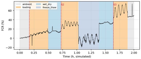
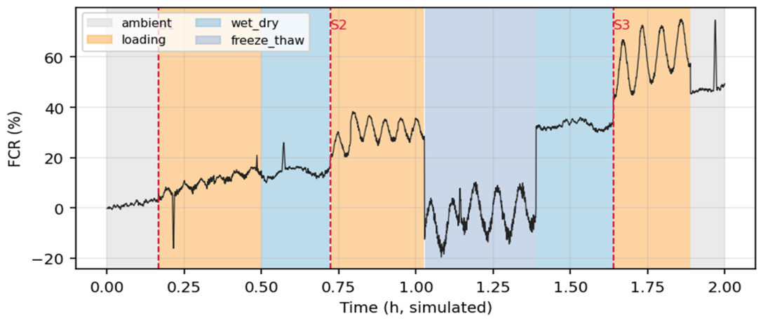
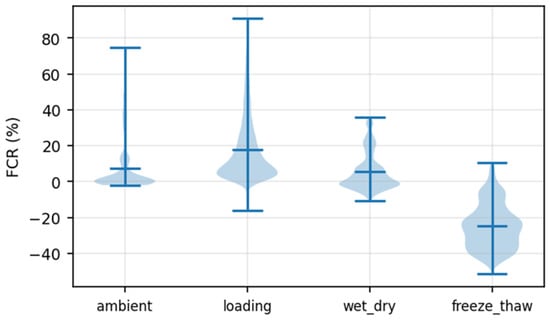
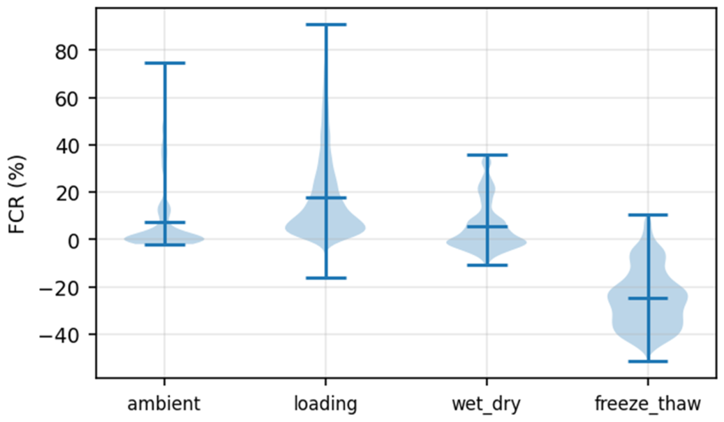
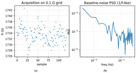
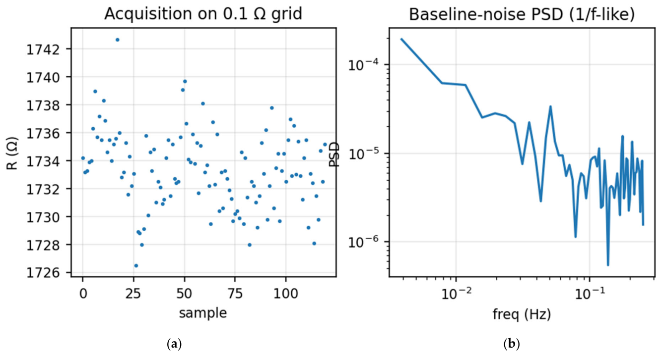
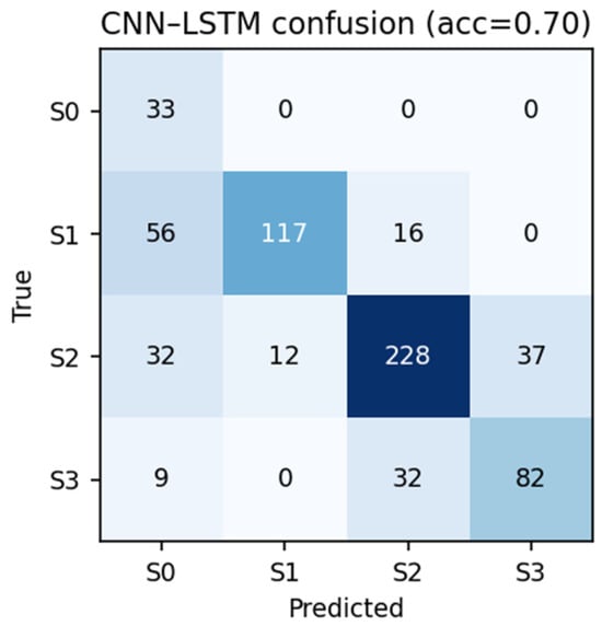
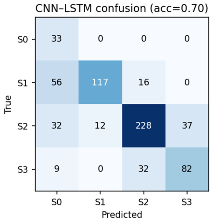
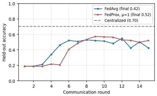
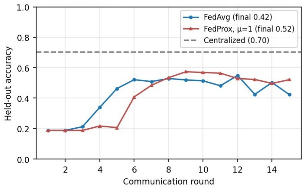
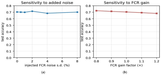
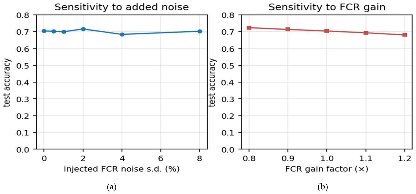

Disclaimer/Publisher’s Note: The statements, opinions and data contained in all publications are solely those of the individual author(s) and contributor(s) and not of MDPI and/or the editor(s). MDPI and/or the editor(s) disclaim responsibility for any injury to people or property resulting from any ideas, methods, instructions or products referred to in the content. |
© 2026 by the authors. Licensee MDPI, Basel, Switzerland. This article is an open access article distributed under the terms and conditions of the Creative Commons Attribution (CC BY) license.