Design and Field Evaluation of a Low-Cost Micro-Meteorological Sensing and Machine-Learning Framework for Hourly Photovoltaic Power Estimation

Abstract

This study presents the design and field evaluation of a low-cost micro-meteorological sensing and machine-learning framework for hourly photovoltaic (PV) power estimation. A 545 W PV module and 750 W grid-tie inverter were instrumented with a NodeMCU ESP8266-based acquisition system integrating local weather sensing and electrical power measurement. Five-minute field observations collected from 1 January to 3 September 2026 were aggregated to hourly resolution with gap-aware processing. Of 5899 candidate hourly timestamps, 5770 model-ready observations were retained (97.81%). Current-hour target power P(t) was estimated using contemporaneous sensing and preceding-hour power P(t − 1), with chronological 64/16/20 training/validation/test partitions and training-only preprocessing. The primary, ten-seed, three-input BPNN (illuminance, temperature, and preceding-hour power) achieved all-hours MAE 11.02 ± 0.88 W (mean ± sample SD), outperforming a three-input XGBoost (version 3.4.1) comparison (14.80 ± 0.20 W). Ten-seed paired MAE improvement was 3.79 ± 0.96 W, with a hierarchical moving-block bootstrap 95% interval of 2.90–4.63 W for the fixed test period. The full five-input BPNN was less accurate (12.52 ± 1.82 W); humidity and pressure did not improve average accuracy at this site. The original single-run BPNN MAE of 11.11 W was retained only as a separate historical comparison. The contribution was an auditable field-deployed estimation workflow rather than a new learning algorithm or validated on-device inference. The three-input BPNN was the recommended configuration. The five-input model remained a feature-ablation and full-feature baseline, not the principal performance claim. The estimated-power reference may complement direct PZEM-004T measurements; fault-detection accuracy, on-device inference, and generalization beyond the studied site were not evaluated. In the separate QC-cleaned ten-seed sensitivity analysis, all 1145 test hours fell within the observed training target-power range (0–349.92 W), yet MAE increased from 7.69 ± 0.88 W at ≤250 W to 29.24 ± 3.83 W above 250 W; reliability at high power remained limited.

1. Introduction

Photovoltaic (PV) generation varies with local solar input, temperature, humidity, atmospheric conditions, shading, and short-term environmental changes. Forecasting and estimation studies therefore depend strongly on data source, forecast horizon, predictor availability, and evaluation design [1,2,3]. For small distributed PV installations, localized sensing can reduce the spatial mismatch between regional weather observations and the conditions experienced by the module.

Artificial-intelligence methods have long been applied to PV systems because nonlinear models can represent complex relationships between environmental variables and electrical output [2]. More recent work has applied machine learning to solar-irradiance and temperature prediction for PV applications [4], while renewable-energy-community studies have demonstrated the operational value of data-driven energy estimates and forecasts [5]. However, model accuracy alone does not establish the engineering value of a field monitoring system; the task definition, temporal split, missing-data handling, baseline selection, and treatment of nighttime zero-power periods must also be explicit.

Low-cost Internet of Things (IoT) platforms provide a practical route to localized PV monitoring. Field studies have combined environmental and electrical sensing with IoT acquisition [6,7], and ANN-assisted systems have been investigated for PV condition and soiling assessment [8]. These studies support the feasibility of low-cost sensing and machine learning, but they do not remove the need for an auditable sensing-to-model workflow under real data interruptions.

The recent literature reinforces both the relevance and the limitations of low-cost PV sensing. Nkinyam et al. [9] reported a remotely accessible IoT PV monitoring device, while Nava-Pintor et al. [10] evaluated inexpensive photometric sensors against a dedicated solar-radiation reference using regression and machine-learning calibration. A 2026 low-cost irradiance soft-sensor study [11] combined PV electrical measurements with solar geometry and reference-pyranometer validation. These studies demonstrate that affordable instrumentation and data-driven estimation are established approaches; the present study therefore does not claim novelty from IoT connectivity or neural networks alone.

Other recent systems have pursued different measurement targets and verification levels. Rhiat et al. [12] embedded an ANN-based irradiance meter on an ESP8266 and compared it with a commercial irradiance meter. Nafa et al. [13] examined sensorless irradiance estimation using PV electrical quantities and a simulation-based MPPT framework. Srisiri et al. [14] investigated fault classification using an open-source PV monitoring platform with labeled faults, whereas the present work evaluates expected hourly AC power and has not validated a fault classifier. A 2026 systematic review [15] emphasizes the importance of evaluating uncertainty, deployment conditions, and cost-effectiveness in low-cost PV monitoring. The comparison below distinguishes measured quantity, field validation, and monitoring purpose rather than directly comparing incompatible error metrics.

Relative to the heterogeneous sensing, irradiance-estimation, and PV-monitoring studies summarized in Table 1, this study combines a field-deployed 545 W PV sensing system with gap-aware five-minute-to-hourly data construction, strictly chronological evaluation, and matched-seed BPNN/XGBoost comparisons for current-hour AC power estimation. Its distinctive empirical finding is that an illuminance–temperature–previous-hour-power model outperformed the humidity/pressure-augmented alternative at this single site; no novel neural-network algorithm, calibrated irradiance measurement, or validated fault detector is claimed.

Table 1. Comparison with selected recent low-cost photovoltaic sensing and monitoring studies.

Study	Sensing/Estimated Target	Validation/Approach	Distinction from This Study
Nkinyam et al. (2025) [9]	IoT-based PV electrical monitoring	Development of a remotely accessible low-cost monitoring device	Monitors measured PV operating quantities; does not establish the same lagged-power, hourly AC-output estimation task.
Nava-Pintor et al. (2025) [10]	Low-cost light sensors for solar-radiation estimation	Sensor evaluation against a solar-radiation reference; regression/ML calibration	Addresses optical-sensor calibration for radiation, rather than estimating hourly inverter AC power.
Voicu and Petreuș (2026) [11]	Global horizontal irradiance soft sensing	Hybrid physical/ML estimation from a low-cost PV measurement platform	Estimates irradiance rather than measured inverter AC output; different target and validation basis.
Rhiat et al. (2026) [12]	ANN-enhanced solar irradiance meter	IoT/ANN irradiance-meter design and comparison with a commercial instrument	Focuses on an irradiance measuring instrument, not a lagged-power AC-output reference.
Nafa et al. (2025) [13]	Sensorless solar irradiance estimation	PV electrical inputs and PSO-MPPT/IoT-enabled monitoring framework	Targets irradiance using PV electrical behavior, rather than measured hourly AC power from local micro-weather and lagged power.
Srisiri et al. (2026) [14]	PV fault classification	AI-based fault classification with a low-cost open-source IoT platform	Validates fault classes; the present work estimates expected AC power and does not validate fault classification.
Jundi et al. (2026) [15]	Low-cost PV monitoring technologies	Systematic literature review of technologies and challenges	Synthesizes prior systems; the present study reports one deployed system with a chronological evaluation.

Research contributions and feature selection. The principal contribution is the design, implementation, and single-site field evaluation of a low-cost IoT-based micro-meteorological sensing and hourly PV power estimation workflow. In ten-seed BPNN experiments, the three-feature configuration (illuminance, ambient temperature, and previous-hour PV power) achieved a lower mean test MAE (11.02 ± 0.88 W) than the five-feature configuration (12.52 ± 1.82 W). Under the investigated conditions, adding humidity and atmospheric pressure did not improve mean predictive accuracy. This work does not propose a new BPNN algorithm or establish superiority over publicly available meteorological data.

The PZEM-004T provides measured AC output power, whereas the BPNN estimates expected current-hour power from micro-meteorological observations and exact previous-hour measured power. Comparing these complementary quantities may flag periods requiring investigation for abnormal operation or data-acquisition inconsistencies. This study validates estimation accuracy; it does not validate automated fault detection or identify fault causes.

2. System Design and Field Deployment

2.1. Integrated Sensing Architecture

The field platform consists of an operational 545 W PV module connected to a 750 W grid-tie inverter. A NodeMCU ESP8266 microcontroller serves as the local acquisition node. An AHT10 measures ambient temperature and relative humidity, a BMP180 measures barometric pressure, and a BH1750 provides an illuminance-derived proxy for incident solar input. A PZEM-004T module provides electrical measurements. The BH1750-derived quantity is treated conservatively as a radiation proxy rather than as calibrated pyranometer irradiance. The main sensing components and their functions are summarized in Table 2.

Table 2. Integrated field sensing system components and roles.

Component	Role	Measurement/Function	Model/Manufacturer
545 W PV module	Energy source	Field PV generation	LR5-72HPH-545M, LONGi Solar, Xi’an, China
750 W grid-tie inverter	Power conversion	PV-to-grid conversion	Y&H Grid Tie Micro Inverter, Shenzhen, China
NodeMCU ESP8266	Acquisition node	Sensor polling and local data transfer	Espressif Systems, Shanghai, China
AHT10	Micro-meteorological sensing	Temperature and relative humidity	Aosong Electronics, Guangzhou, China
BMP180	Micro-meteorological sensing	Barometric pressure	Bosch Sensortec, Kusterdingen, Germany
BH1750	Optical sensing	Illuminance-derived solar-input proxy	ROHM Semiconductor, Kyoto, Japan
PZEM-004T	Electrical sensing	Electrical power measurements	Ningbo Peacefair Electronic Technology Co., Ltd., Ningbo, China

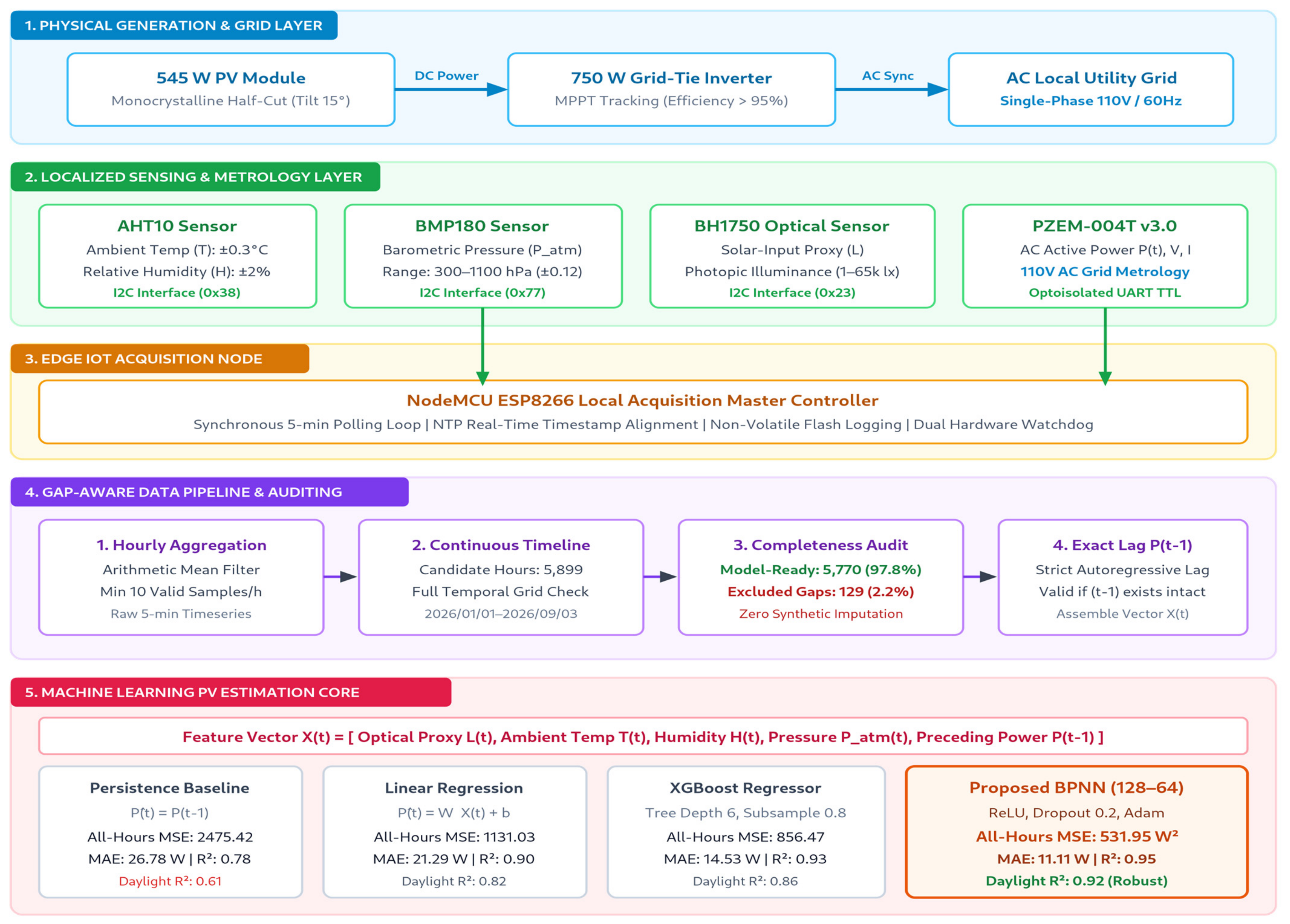
The electrical meter supplies the observed power used for model training and evaluation. The BPNN supplies an expected-power reference for potential residual-based monitoring. Because preceding-hour measured power is a model input, the reference is not fully independent of the PZEM-004T. A large residual is an anomaly candidate, not proof of hardware failure. The integrated field sensing and estimation framework is illustrated in Figure 1.

Figure 1. Integrated field sensing, data acquisition, and machine-learning PV estimation framework.

2.2. Acquisition and Data Path

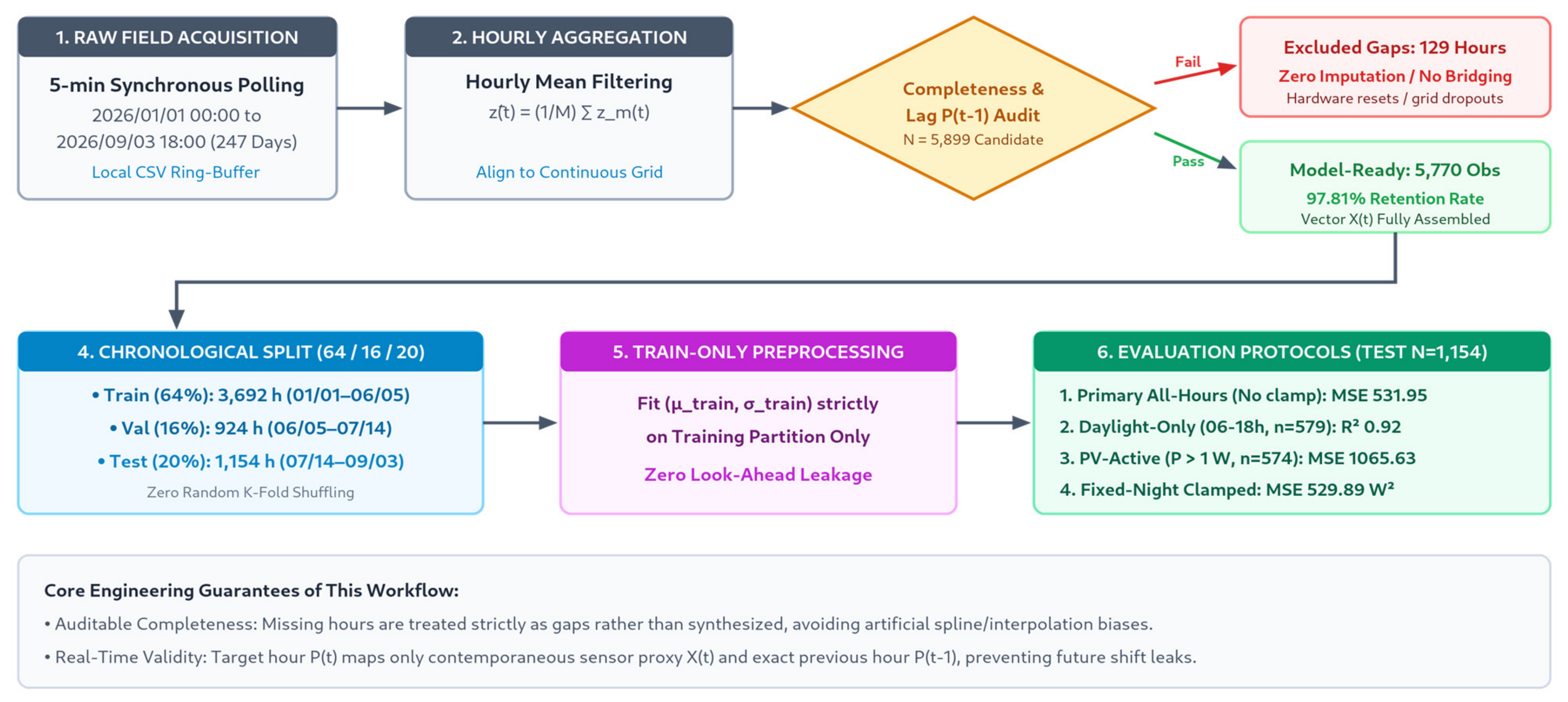
Synchronous field measurements were recorded at five-minute resolution and stored locally. Five-minute records were subsequently aggregated to hourly resolution. A continuous hourly timeline was used during data construction so that missing intervals were exposed explicitly. A current-hour observation was retained only when the target power and all required micro-meteorological inputs were complete, and the lagged-power feature was accepted only when the exact preceding hourly timestamp was available. The complete data construction and evaluation workflow is illustrated in Figure 2.

Figure 2. Gap-aware data construction, chronological splitting, preprocessing, and model-evaluation workflow.

2.3. Physical Testbed and Electrical Configuration

The experimental platform was deployed at a residential field test site along Section 4 of Zhonghua Road in Xiangshan District, Hsinchu City, Taiwan. The field location is approximately 24.7891° N, 120.9329° E (WGS84). These coordinates are provided to document the geographic context of the field measurements and support the reproducibility of site-specific micro-meteorological observations.

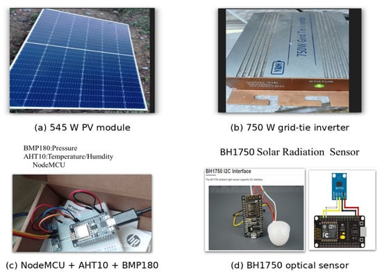
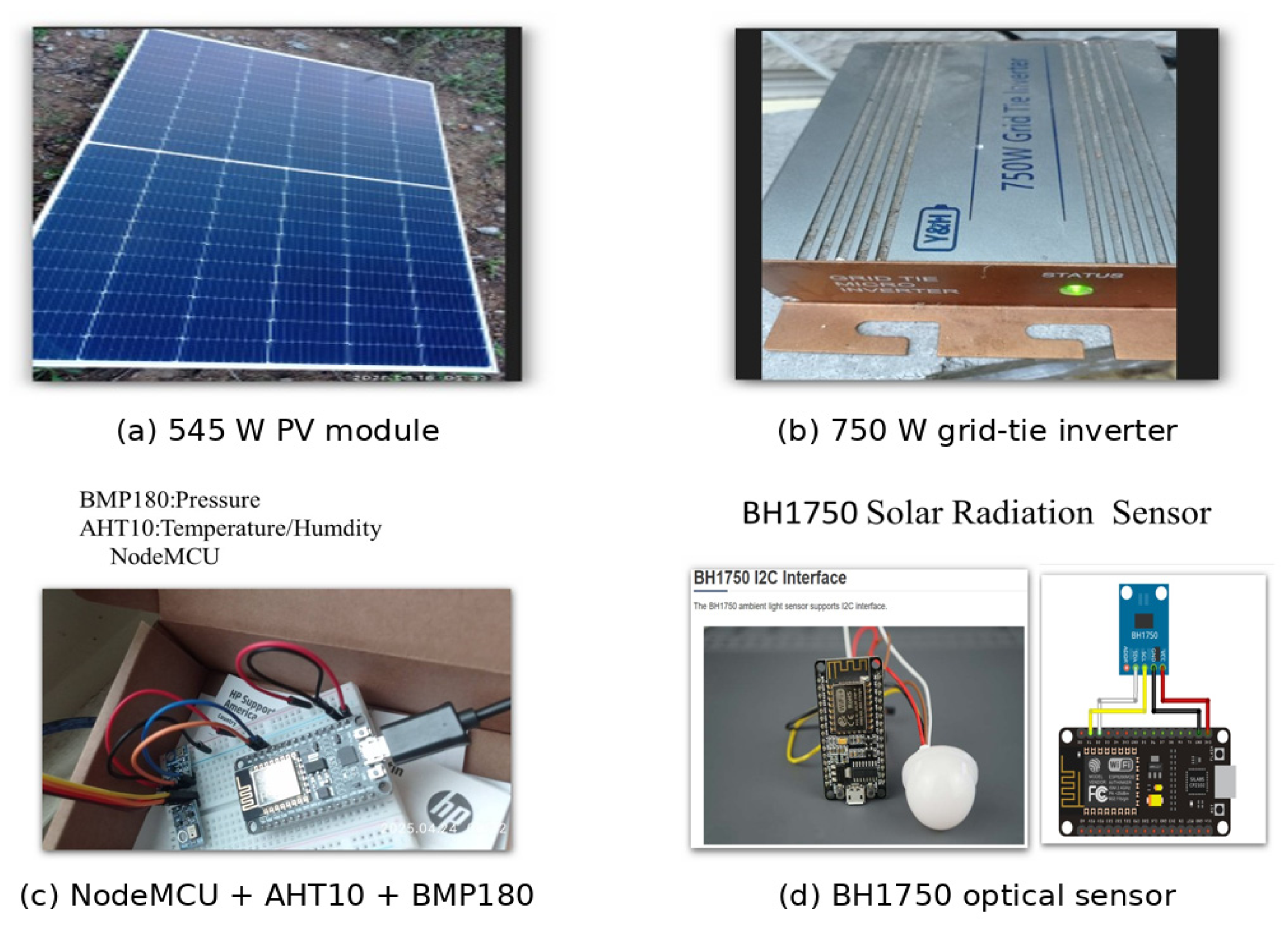
The generation system comprises a single 545 W monocrystalline-silicon PV module installed at 24.7891° N, 120.9329° E (WGS84), Section 4 of Zhonghua Road in Xiangshan District, Hsinchu City, Taiwan, at a tilt angle of approximately 6.2° relative to the horizontal plane and an azimuth of approximately 263.4° clockwise from geographic north (approximately west-facing, 6.6° south of due west, measured along the downward-facing direction of the tilted module), and connected to a 750 W grid-tie micro-inverter supplying the local single-phase 110 V/60 Hz electrical grid. The field configuration represents a small-scale residential PV installation rather than a utility-scale plant. Electrical output and localized atmospheric variables were acquired synchronously so that each model input corresponded to the same physical operating interval as the measured PV power. Figure 3 documents the principal hardware used in the field installation.

Figure 3. Actual field hardware used in the experimental platform: (a) 545 W PV module; (b) 750 W grid-tie inverter; (c) NodeMCU ESP8266 with AHT10 and BMP180 sensing modules; and (d) BH1750 optical sensing module.

2.4. Micro-Meteorological and Electrical Metrology

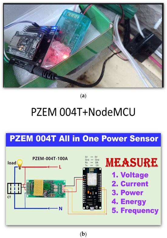
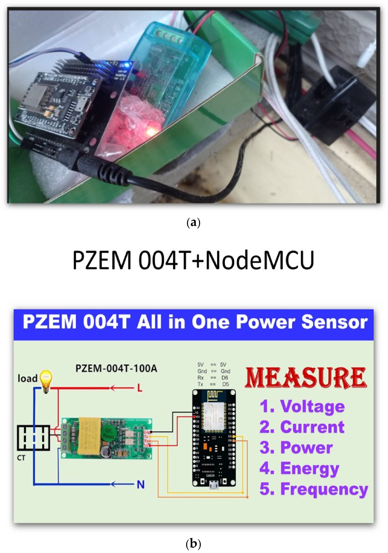
The sensing layer combines low-cost digital devices with isolated electrical metrology. The AHT10 provides ambient temperature and relative humidity through the I2C bus, while the BMP180 provides barometric pressure. The BH1750 measures photopic illuminance and is used only as an illuminance-derived solar-input proxy; it is not treated as equivalent to broadband irradiance measured by an ISO-class thermopile pyranometer. The PZEM-004T v3.0 is connected to the local single-phase 110 V AC circuit and provides active AC power together with line-voltage/current information through an optically isolated serial interface. This distinction between an optical proxy and calibrated irradiance is maintained throughout the analysis to avoid overstating measurement accuracy. The installed Peacefair PZEM-004T module is paired with a 100 A split-core current transformer and communicates over TTL UART using Modbus-RTU. The electrical metrology integration is illustrated in Figure 4. The manufacturer-specified measurement ranges for the described PZEM-004T variant are 80–260 V AC, 0–100 A, 0–23 kW active power, 0–9999 kWh energy, 45–65 Hz frequency, and 0.00–1.00 power factor, with a nominal Class 1.0 (±1.0%) accuracy specification. These nominal specifications are not a substitute for independent calibration of the installed unit.

Figure 4. PZEM-004T electrical metrology integration: (a) actual PZEM-004T/NodeMCU field installation; (b) PZEM-004T connection and measured electrical quantities used as an implementation reference.

The NodeMCU ESP8266 acts as the acquisition controller and coordinates periodic sensor polling, timestamp synchronization, and local data storage. The hardware design emphasizes low component count and practical field maintainability. Although the architecture is compatible with embedded inference, the present study evaluates the sensing-to-estimation pipeline rather than claiming a measured on-device inference benchmark.

2.5. Hardware Components and Design Rationale

The field instrumentation was selected to balance localized measurement capability, electrical isolation, low component count, replacement availability, and practical deployment cost. The NodeMCU ESP8266 integrates Wi-Fi connectivity and common embedded communication interfaces in a compact controller. The AHT10 and BMP180 provide digital temperature/humidity and barometric-pressure measurements through I2C, reducing analog signal-conditioning requirements. The BH1750 provides a digital photopic illuminance measurement and is used in this study only as an illuminance-derived solar-input proxy; it is not considered a substitute for a calibrated broadband pyranometer. The PZEM-004T v3.0 provides AC electrical measurements on the 110 V grid-side circuit through an isolated serial measurement interface, allowing the low-voltage acquisition controller to remain separated from the grid-side measurement circuit. These design choices prioritize a reproducible small-scale field platform rather than laboratory-grade metrology. The hardware interfaces, design rationale, and limitations are summarized in Table 3.

Table 3. Hardware components, interfaces, design rationale, and limitations.

Component	Measured/Controlled Quantity	Interface/Role	Design Rationale	Important Limitation
NodeMCU ESP8266	Acquisition, timing, local communication	I2C/serial/Wi-Fi controller	Low-cost integrated controller; compact and easily replaceable	Not an industrial PLC; embedded inference performance was not benchmarked
AHT10	Ambient temperature and relative humidity	Digital I2C sensor	Direct digital micro-meteorological sensing with simple integration	Consumer/embedded sensor class; requires suitable enclosure and placement
BMP180	Barometric pressure	Digital I2C sensor	Adds local atmospheric-pressure information with minimal wiring	Legacy low-cost sensor; not a reference-grade barometer
BH1750	Photopic illuminance	Digital I2C optical sensor	Low-cost localized optical proxy located near the PV system	Spectral response differs from a thermopile pyranometer; not calibrated irradiance
PZEM-004T v3.0	AC voltage (80–260 V), current (0–100 A), active power (0–23 kW), energy, frequency and power factor	100 A split-core CT; TTL UART/Modbus-RTU	Provides synchronized electrical output for model target construction	Nominal Class 1.0 (±1.0%); not independently calibrated; not revenue-grade metrology
545 W PV module + 750 W inverter	PV generation and grid conversion	Physical energy layer	Representative small distributed PV testbed	Single-module/single-site scale limits external generalization

2.5.1. Photovoltaic Module Specifications

The field testbed uses a LONGi Hi-MO 5m LR5-72HPH-545M monocrystalline PV module. According to the manufacturer datasheet, the 545 W variant has the following STC electrical and mechanical characteristics [16]. These specifications define the physical generation asset used in the experiment; the machine-learning target remains the measured field power rather than the module nameplate rating.The manufacturer’s specifications of the PV module are summarized in Table 4.

Table 4. Manufacturer specifications of the 545 W PV module used in the field testbed.

Parameter	545 W Module Specification	Condition/Note
Model	LR5-72HPH-545M	LONGi Hi-MO 5m
Maximum power, Pmax	545 W	STC
Open-circuit voltage, Voc	49.65 V	STC
Short-circuit current, Isc	13.92 A	STC
Voltage at maximum power, Vmp	41.80 V	STC
Current at maximum power, Imp	13.04 A	STC
Module efficiency	21.1%	STC
Power tolerance	0 to +3%	Manufacturer rating
Dimensions	2278 × 1134 × 35 mm	Mechanical
Weight	27.5 kg	Mechanical
Operating temperature	−40 to +85 °C	Operating range
Maximum system voltage	DC 1500 V	IEC/UL
Temperature coefficient of Pmax	−0.340%/°C	STC rating

Source: LONGi manufacturer’s datasheet [16].

2.5.2. Prototype Sensing and Acquisition Cost

To make the low-cost claim auditable, Table 5 reports the approximate prototype acquisition cost of the sensing and acquisition hardware. The values correspond to the component-level bill of materials used during prototype construction and are intended as an engineering cost basis rather than a universal market quotation. The PV module and grid-tie inverter are excluded because they constitute the generation testbed rather than the monitoring subsystem; taxes, shipping, calibration services, and labor are also excluded.

Table 5. Approximate prototype bill of materials for the low-cost monitoring subsystem.

Monitoring Component	Approx. Unit Cost (USD)	Function
NodeMCU ESP8266	4.50	Acquisition controller/Wi-Fi
AHT10	1.80	Temperature and relative humidity
BMP180	1.50	Barometric pressure
BH1750	2.20	Illuminance-derived solar-input proxy
PZEM-004T v3.0	12.00	Peacefair meter with 100 A split-core CT; AC electrical metrology
Ancillary hardware (estimated)	9.50	Power supply, enclosure, wiring and connectors; residual prototype estimate
Total monitoring BOM (estimated)	31.50	Five electronic modules (USD 22.00) + ancillary materials (USD 9.50)

The five electronic modules total USD 22.00, including the PZEM-004T at approximately USD 12.00 (local procurement of approximately NTD 380, inclusive of a 100 A split-core current transformer). An additional USD 9.50 is allocated to ancillary prototype materials such as the power supply, wiring, connectors, and enclosure, giving an estimated component BOM of USD 31.50 (including the estimated USD 9.50 ancillary-material allocation). The USD 9.50 is a residual estimate based on the original prototype total, not an independently itemized purchase ledger. The PV module, inverter, shipping, labor, installation, and calibration services are excluded.

2.6. Engineering Trade-Offs Versus Commercial-Grade Monitoring Equipment

The proposed platform is not intended to replace calibrated utility-scale meteorological or power-quality instrumentation, including solar-radiation instruments classified under ISO 9060:2018 [17]. Its design objective is different: to obtain synchronized, site-localized variables at sufficiently high temporal resolution for field evaluation of PV estimation models using inexpensive and readily replaceable components. The five electronic modules cost approximately USD 22.00, and ancillary prototype materials add an estimated USD 9.50, yielding a total monitoring-subsystem materials cost of approximately USD 31.50 (Table 5). This estimate excludes the PV module, inverter, labor, shipping, installation, and calibration services. Commercial-grade monitoring stations generally incur substantially higher equipment and commissioning costs because they incorporate calibrated radiometers, industrial data loggers, environmental enclosures, traceable calibration, and long-term support; because vendor configurations and service scopes vary widely, this study does not assign a single unsupported commercial-system price. The resulting trade-off is therefore affordability and experimental flexibility versus metrological traceability and industrial robustness. The engineering trade-offs are summarized in Table 6. This distinction is especially important for the BH1750, whose illuminance response cannot be interpreted as ISO-class broadband solar irradiance.

Table 6. Engineering trade-offs between the proposed low-cost field platform and commercial/professional monitoring systems.

Criterion	Proposed Low-Cost Field Platform	Commercial/Professional Monitoring System
Primary objective	Localized research sensing and ML data acquisition	Traceable meteorological/electrical monitoring and plant operation
Acquisition architecture	Open, component-level NodeMCU/sensor integration	Integrated data logger, industrial controller, or vendor ecosystem
Solar-input measurement	BH1750 illuminance-derived proxy	Calibrated pyranometer/reference irradiance sensor
Electrical measurement	PZEM-004T class low-cost electrical metrology	Revenue-/industrial-grade meter or power-quality analyzer
Deployment cost	Low; commodity components and simple replacement	Higher; calibrated sensors, logger, enclosure, commissioning and maintenance
Customization	High; firmware, sampling and feature pipeline are directly modifiable	Usually structured around vendor-supported channels/software
Calibration traceability	Limited unless independently calibrated	Typically stronger and documented
Environmental robustness	Depends on enclosure, installation and component protection	Designed for long-term outdoor/industrial operation
Best-fit use	Research prototypes, distributed small PV, teaching and localized ML studies	Utility/commercial PV monitoring, compliance, bankable performance assessment

The comparison above is a design-level comparison rather than a claim of superior measurement accuracy; low-cost IoT monitoring remains useful for localized research applications [6,7], while standardized radiometry serves a different metrological purpose [17]. For this reason, model results are interpreted within the limitations of the installed sensor class, and future work should validate the optical proxy against calibrated irradiance instrumentation and assess longer-term sensor drift.

3. Materials and Methods

3.1. Dataset Construction and Completeness Audit

During long-term field operation, occasional data gaps occurred because of temporary power outages, sensor or acquisition-node malfunctions, data-collector crashes or automatic resets, and communication interruptions (e.g., Wi-Fi or network failures). These events could stop the NodeMCU/acquisition system from recording or transmitting valid measurements and therefore produced missing or incomplete time intervals. The missing intervals were preserved as explicit gaps rather than filled by interpolation or carry-forward methods. After alignment, completeness screening, and exact-lag construction, 5770 of 5899 candidate hourly timestamps were retained (97.81%), while 129 timestamps were excluded from the model-ready dataset. The excluded timestamps should not be interpreted as outlier removal; they reflect unavailable or incomplete field measurements and exact-lag requirements.

The 129 excluded hours were unevenly distributed across the observation period: January 7, February 0, March 1, April 32, May 0, June 1, July 43, August 45, and September 0 (through 3 September 2026, 18:00). July and August accounted for 88/129 (68.2%) exclusions. This establishes temporal clustering, but the monthly ledger alone does not identify the physical cause of each gap. The counts are descriptive, not evidence that missingness was random or missing completely at random. The monthly data completeness audit is presented in Table 7.

Table 7. Field data completeness audit ledger.

Month (2026)	Candidate Hours	Retained Hours	Excluded Hours	Retention (%)
2026-01	744	737	7	99.06
2026-02	672	672	0	100.00
2026-03	744	743	1	99.87
2026-04	720	688	32	95.56
2026-05	744	744	0	100.00
2026-06	720	719	1	99.86
2026-07	744	701	43	94.22
2026-08	744	699	45	93.95
2026-09	67	67	0	100.00
Audit Item		Value
Candidate hourly timestamps		5899
Model-ready observations		5770
Excluded timestamps		129
Retention rate		97.81%
Analysis period		1 January 2026 00:00–3 September 2026 18:00

3.1.1. Field Acquisition and Temporal Aggregation

BH1750 installation and acquisition configuration: The BH1750 light-sensitive surface was mounted horizontally facing upward and operated in continuous high-resolution mode. The acquisition firmware did not explicitly set the BH1750 measurement-time register (MTreg); therefore, no independently verified MTreg value is claimed. The nominal sensor polling interval was five seconds, whereas the analysis used available five-minute observations. Its output is photopic illuminance (lux), not calibrated broadband solar irradiance (W/m²). Measurement timestamps were recorded in Taiwan Standard Time (UTC + 08:00). In the source aggregation code, inverter timestamps (time) and weather reception timestamps (received_time) were independently floored to the beginning of each hour using dt.floor(“h”), and each variable was averaged within its hourly group. Thus, a record labeled 11:00 represents measurements timestamped from 11:00:00 through 11:59:59 (UTC + 08:00). Although the time zone is specified, the clock synchronization accuracy between the two acquisition sources was not independently verified. No fixed minimum number of valid five-minute samples per hour was imposed; missing samples were not interpolated. A translucent white dome-shaped cover was installed over the BH1750 throughout the field measurement period (Figure 3d). The cover provided physical protection and may have altered optical transmission and angular response; its transmittance and angular characteristics were not independently calibrated. Therefore, the recorded maximum of 37,450 lux cannot be quantitatively attributed to the cover, and the measured lux values represent installation-dependent optical readings. The AHT10 temperature and humidity sensor was operated without a radiation shield. Its temperature readings may therefore be affected by direct solar heating, particularly under strong sunlight.

The sensing and inverter data streams were acquired at nominal five-minute resolution and aligned by their recorded hourly timestamps; independent clock synchronization accuracy was not verified. Hourly observations were constructed by averaging the available valid five-minute measurements within each hourly interval. No fixed minimum number of valid five-minute samples per hour was imposed during hourly aggregation. Rather than creating a visually continuous series by interpolation, the processing workflow first generated a continuous hourly timestamp index and then audited the availability of the required measurements at each timestamp. This makes acquisition failures visible and prevents missing intervals from being silently converted into synthetic observations.

Retrospective BH1750 sample-count audit: Of 5770 retained modeling hours, 5739 (99.46%) contained at least ten valid illuminance records; 31 contained fewer than ten, including four hours with only one record. These counts describe acquisition completeness and were not used as an eligibility filter in the original modeling pipeline. Consequently, hourly means based on sparse observations may be less representative of conditions throughout the hour. Future work will implement and prospectively validate a minimum valid-sample threshold before chronological data splitting, quantify sensitivity to alternative thresholds, and repeat model training and evaluation on the resulting quality-controlled data.

Supplementary quality-controlled retraining audit (performed after the original analysis): A retrospective sensitivity experiment required at least 10 valid BH1750 readings per hour and excluded the four independently flagged 31 August low-illuminance/high-power observations. The criteria excluded 35 of 5770 original model-ready observations (31 sparse-sample hours and four flagged hours), leaving 5735 observations. These thresholds were not part of the original data-construction protocol, and the original results remain unchanged. This is a retrospective sensitivity experiment, not evidence that the threshold was prospectively prespecified.

3.1.2. Exact-Lag Pairing and Gap Handling

For each candidate hour t, the current environmental vector and target PV power were checked for completeness. The lagged power feature was joined by its exact timestamp t − 1 h. A sample was rejected when the required preceding-hour observation was unavailable; the algorithm did not substitute the most recent available earlier observation. Consequently, the lag feature preserves its physical meaning as exactly one hour of historical power rather than an irregular-duration carry-forward value.

3.2. Current-Hour Estimation Task

The task is current-hour PV power estimation rather than one-hour-ahead forecasting. For each hour t, the input vector comprises the illuminance-derived solar-input proxy L(t), ambient temperature T(t), relative humidity H(t), barometric pressure P_atm(t), and exact preceding-hour PV power P_gen(t − 1). The feature vector is defined as

X(t) = [L(t), T(t), H(t), P_atm(t), P_gen(t − 1)]

(1)

P_gen(t) = f(X(t)) + ε(t)

(2)

Here, f denotes the fitted regression mapping from the five-dimensional input vector X(t) to current-hour AC power, and ε(t) denotes the residual error. P_gen(t) is the measured AC output power at hour t, whereas P_gen(t − 1) is the observed output from exactly one hour earlier. No target shift to t + 1 is applied; therefore, the formulation is current-hour estimation rather than forward forecasting.

This distinction is important because contemporaneous meteorological measurements at hour t are not available in a genuine one-hour-ahead forecast unless they are themselves forecasted. The present formulation is therefore described consistently as current-hour estimation. The forecasting literature is used to contextualize PV modeling methods [1,2,3], but the experimental target in this study remains P(t), not P(t + 1).

3.3. Chronological Split and Preprocessing

Supplementary quality-controlled retraining retained the original chronological boundary timestamps (5 June 2026 12:00 and 14 July 2026 18:00). The original 3692/924/1154 training/validation/test counts became 3669/921/1145 after exclusion (23/3/9 fewer observations, respectively). Quality control was applied before fitting scalers and models; scaling parameters were estimated from each corresponding training partition only. The previous-power feature was joined to the exact preceding clock hour in the original timestamp series, not shifted to the preceding retained row. Four models (BPNN and XGBoost with three or five inputs) were retrained using seeds 40–49; BPNN training used at most 500 epochs, patience 20, and batch size 32. Comparisons below are supplementary and separate from the original single-run model comparison.

The 5770 model-ready observations were split chronologically into 3692 training samples (64%), 924 validation samples (16%), and 1154 independent test samples (20%). The chronological data partitions are summarized in Table 8. The corresponding periods were 1 January 2026 00:00–5 June 2026 11:00, 5 June 2026 12:00–14 July 2026 17:00, and 14 July 2026 18:00–3 September 2026 18:00. For each input feature x, min_train(x) and max_train(x) denote its minimum and maximum values in the training partition. Equation (3) defines the resulting min–max-scaled feature x_scaled(t); the training-derived scaling parameters were applied unchanged to validation and test data:

x_scaled(t) = [x(t) − min_train(x)]/[max_train(x) − min_train(x)]

(3)

Table 8. Chronological train–validation–test split.

Subset	n	Period
Training	3692	1 January 2026 00:00–5 June 2026 11:00
Validation	924	5 June 2026 12:00–14 July 2026 17:00
Test	1154	14 July 2026 18:00–3 September 2026 18:00

3.4. Compared Models

Persistence uses $\hat{\mathrm{P}}$(t) = P(t − 1) and provides a direct autoregressive baseline. Linear regression provides a conventional linear comparator. XGBoost provides a nonlinear gradient-boosted tree comparator based on the scalable tree-boosting framework introduced by Chen and Guestrin [18]. The BPNN is a multilayer feedforward neural network using two hidden layers. All trained models use the same feature definition and chronological evaluation timestamps.

3.5. BPNN Configuration

The principal BPNN architecture (128–64 hidden neurons) was predefined before the architecture sensitivity comparison, rather than selected using held-out test performance. This predefined configuration contains two hidden layers with 128 and 64 neurons, ReLU activation, dropout = 0.20, and a single linear output. Optimization uses Adam with learning rate 0.001 [19]. Early stopping monitors validation loss with patience 20, and a fixed random seed of 42 is used. Four hidden-layer configurations (32–16, 64–32, 128–64, and 256–128) were evaluated under the same data split and preprocessing procedure.

Ten random initializations (seeds 40–49) were evaluated for the complete input set and for feature-ablation configurations using the same 3692/924/1154 chronological partitions and the 128–64 architecture. These supplementary experiments used the exported processed hourly CSV (rounded to two decimal places), whereas the original single-run comparison was fitted to unrounded in-memory hourly aggregates. The two result series are therefore reported separately and should not be treated as bitwise-equivalent reproductions.

3.6. Evaluation Protocol

The primary repeated-training paired comparison uses the same exported processed hourly data, fixed 3692/924/1154 chronological partition, seeds 40–49, and identical 1154 test timestamps for three-input BPNN and three-input XGBoost. For each seed and hour, paired improvement equals the absolute error of XGBoost minus that of BPNN (positive favors BPNN). We summarize ten seed-specific improvements as the mean ± sample SD. A reproducible hierarchical moving-block bootstrap (10,000 replicates; random generator seed 20261014) resamples ten seed labels with replacement and resamples common test-hour blocks of 24 retained consecutive rows with replacement, using the same resampled timestamps for all sampled seeds. This interval reflects model-initialization and serial-sample sensitivity conditional on one site and test period; blocks of retained observations can cross missing clock hours. A one-sided Wilcoxon signed-rank test on the ten seed-level mean improvements is supplementary and does not establish independent seasonal replication. The original single-run comparison is reported separately.

The primary evaluation uses all independent test hours without nighttime output clamping. Additional analyses evaluate daylight hours (06:00–17:59), PV-active hours (measured target power > 1 W), and an optional fixed-nighttime post-processing rule setting estimates to zero during 18:00–05:59. The fixed nighttime rule is treated only as post-processing and not as a novel modeling contribution. Model performance was quantified using mean squared error (MSE), mean absolute error (MAE), and the coefficient of determination (R²), defined as follows:

MSE = (1/n) Σ_i=1ⁿ [y_i − ŷ_i]²

(4)

MAE = (1/n) Σ_i=1ⁿ |y_i − ŷ_i|

(5)

R² = 1 − {Σ_i=1ⁿ [y_i − ŷ_i]²/Σ_i=1ⁿ [y_i − ȳ]²}

(6)

Normalized metrics are computed using the 545 W module nameplate rating as a fixed denominator: nMAE (%) = 100 × MAE/545 W and nRMSE (%) = 100 × √MSE/545 W. For the original BPNN test results, all-hours nMAE = 2.04% and nRMSE = 4.23%; daylight-only nMAE = 3.74% and nRMSE = 5.96%. These nameplate-normalized values do not represent normalization by the observed mean or peak output.

Here, n is the number of observations in the evaluation subset (all test hours, daylight hours, or PV-active hours, as applicable); y_i and ŷ_i are the measured and estimated AC powers (W) for observation i; and ȳ is the mean measured AC power within that same evaluation subset. MSE is reported in W², MAE in W, and R² is dimensionless.

4. Results

4.1. Overall Model Comparison

The recommended three-input BPNN had the lowest ten-seed mean all-hours MAE among the matched three-input BPNN and XGBoost comparisons (11.02 ± 0.88 versus 14.80 ± 0.20 W). The original single-run four-model comparison is retained as a distinct historical benchmark; it should not be interpreted as the primary multi-seed result. The original single-run performance metrics are presented in Table 9.

Table 9. All-hours and daylight performance metrics across evaluated models.

Model	All-Hours MSE (W2)	MAE (W)	R2	Daylight MSE (W2)	MAE (W)	R2
Persistence	2475.42	26.78	0.78	4896.01	51.75	0.61
Linear Regression	1131.03	21.29	0.90	2185.77	34.35	0.82
XGBoost	856.47	14.53	0.93	1705.66	28.68	0.86
BPNN (128–64)	531.95	11.11	0.95	1056.13	20.38	0.92

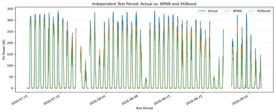
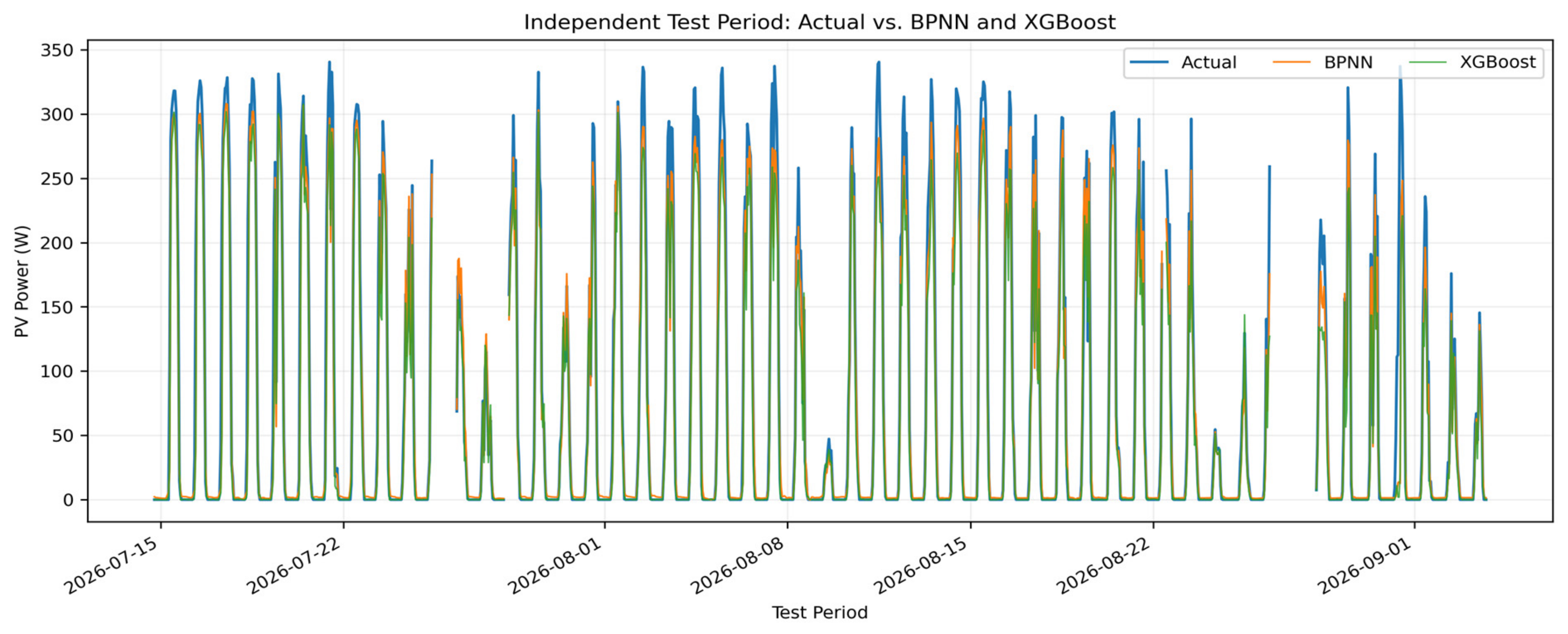
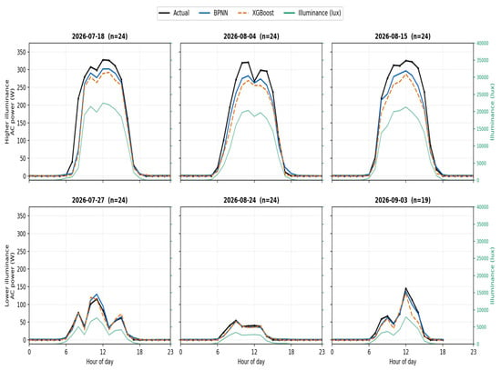
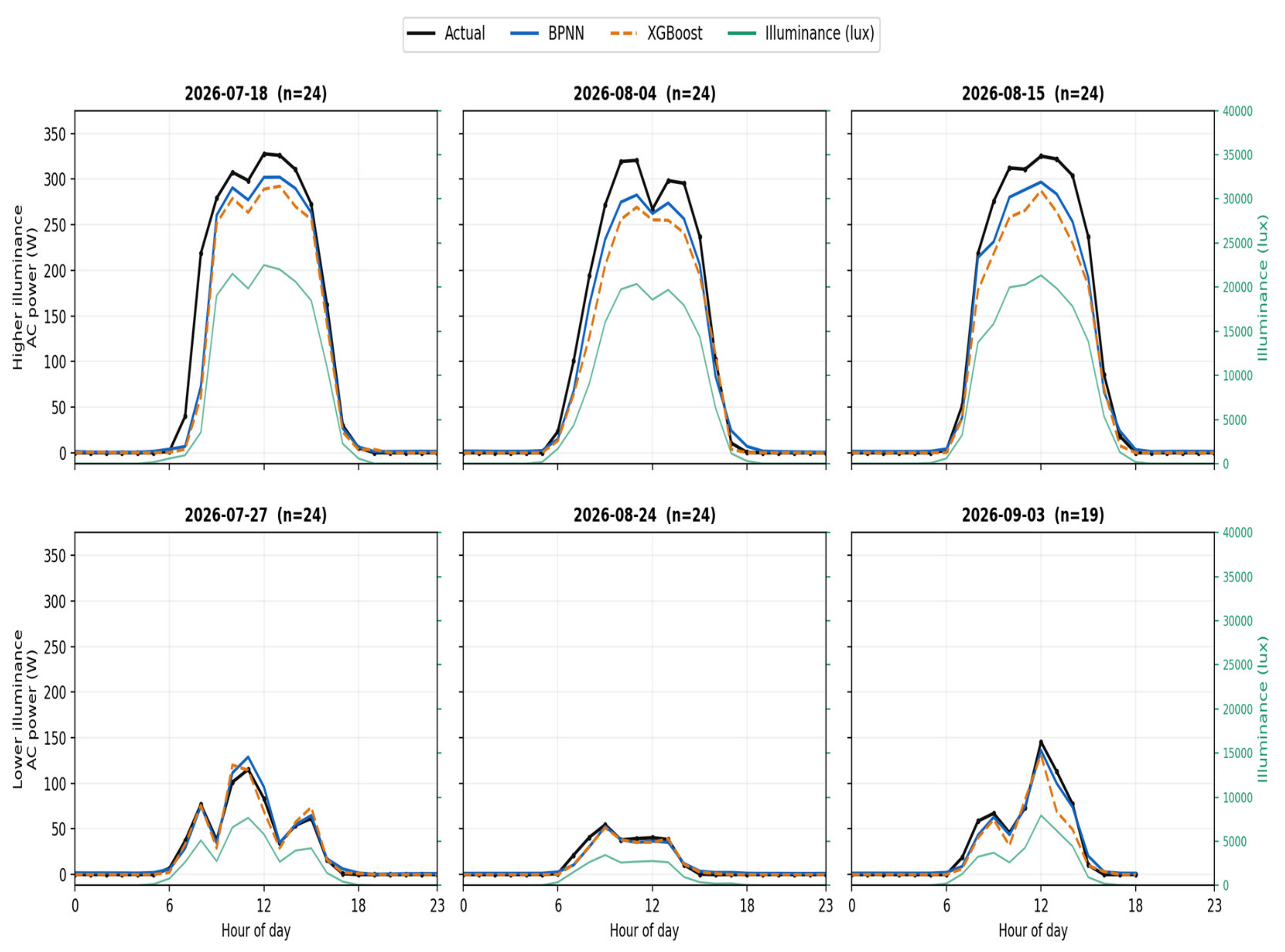
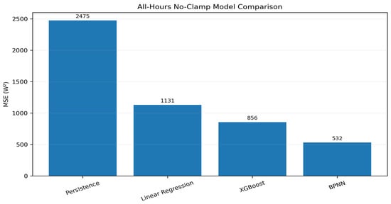
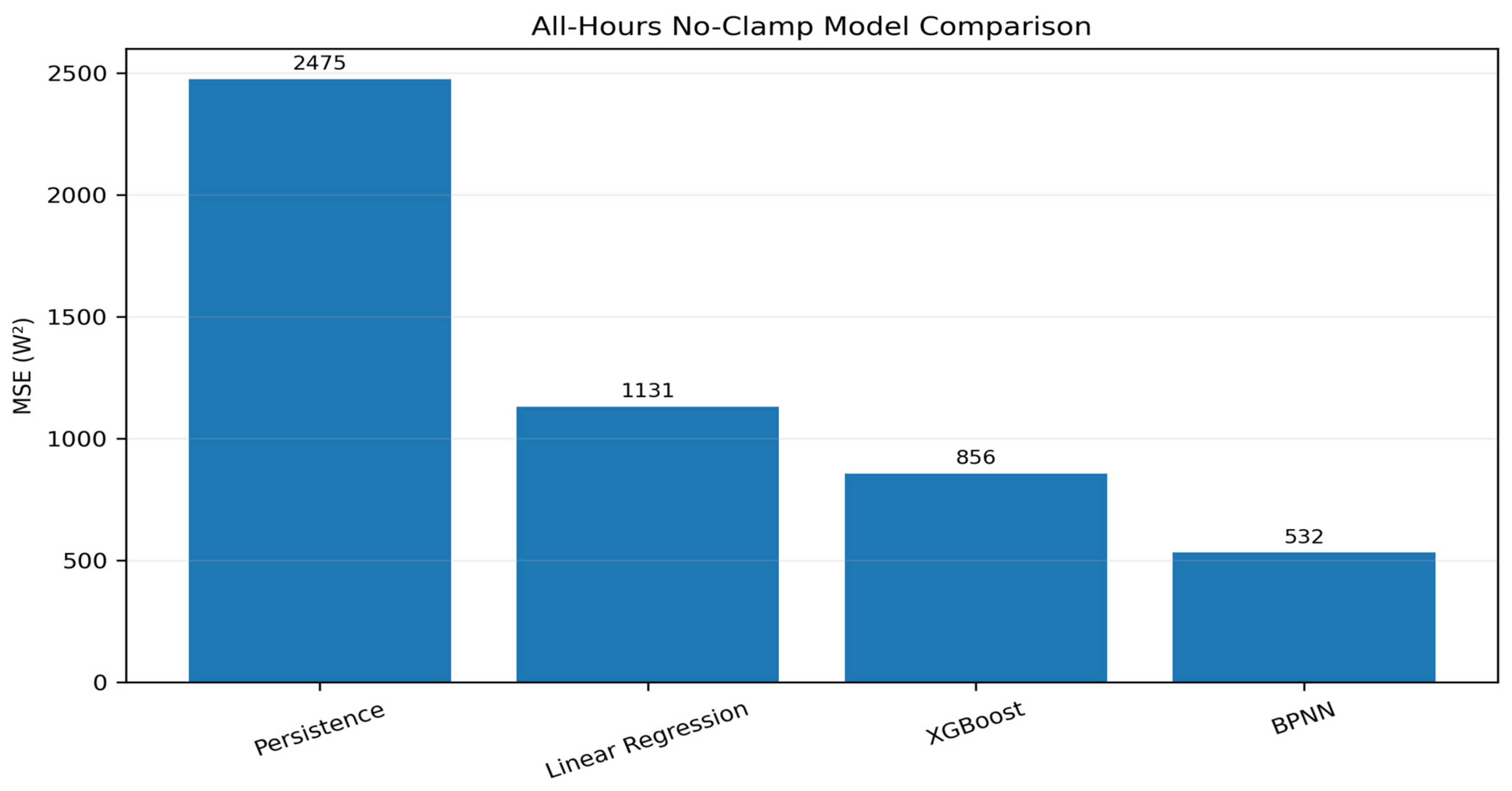
The discontinuities in Figure 5 represent timestamps without valid model-ready observations rather than zero PV generation or model prediction failure. Potential causes include temporary power interruptions, sensor or acquisition malfunctions, data-collector resets, and communication failures; however, the causes of individual gaps were not independently verified. Missing observations were neither interpolated nor bridged, and evaluation was restricted to valid timestamps. Figure 6 presents six representative days from July to September 2026 under contrasting illuminance conditions. Dates are chronological within the higher- and lower-illuminance groups, and the panels use consistent axis scales. The illuminance-based grouping does not imply independently verified clear-sky or cloudy-sky conditions. The corresponding all-hours MSE comparison is illustrated in Figure 7.

Figure 5. Measured AC power and BPNN and XGBoost estimates during the independent held-out test period. Gaps indicate missing or invalid observations.

Figure 6. Measured AC power, BPNN and XGBoost estimates, and illuminance across six representative days. The first three panels represent higher-illuminance conditions, while the last three panels represent lower-illuminance conditions.

Figure 7. All-hours no-clamp MSE comparison across the four evaluated models.

Paired BPNN–XGBoost Comparison

Primary matched-feature multi-seed comparison: on the same 1154 test hours and with identical three-input feature sets, the BPNN achieved MAE 11.02 ± 0.88 W across seeds 40–49 and XGBoost achieved 14.80 ± 0.20 W (mean ± sample SD). The mean seed-level paired absolute-error improvement was 3.79 ± 0.96 W. A 10,000-replicate hierarchical moving-block bootstrap resampling both seeds and common 24-retained-observation time blocks yielded a 95% interval of 2.90–4.63 W; a supplementary one-sided Wilcoxon test of the ten seed-level gains yielded p = 0.00098. For context, the matched five-input comparison gave BPNN 12.52 ± 1.82 W versus XGBoost 14.59 ± 0.14 W, mean paired improvement 2.07 ± 1.74 W and bootstrap interval 0.87–3.44 W. The previously reported original single-run paired comparison (BPNN MAE 11.11 W versus XGBoost 14.53 W, improvement 3.42 W and block-bootstrap interval 2.67–4.24 W) remains an explicitly separate experiment and is not the headline inference. Table 10 retains the original single-run figures for traceability; the multi-seed inference uses the separately archived repeated-training predictions.

Table 10. Paired original experimental test-set model comparison (n = 1154; no nighttime clamping).

Model	MAE (W)	MSE (W2)	RMSE (W)	R2	Bias (W)
BPNN	11.11	531.95	23.06	0.9535	−7.41
XGBoost	14.53	856.47	29.27	0.9252	−13.62

4.2. Daylight and PV-Active Robustness

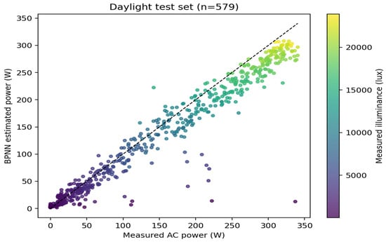
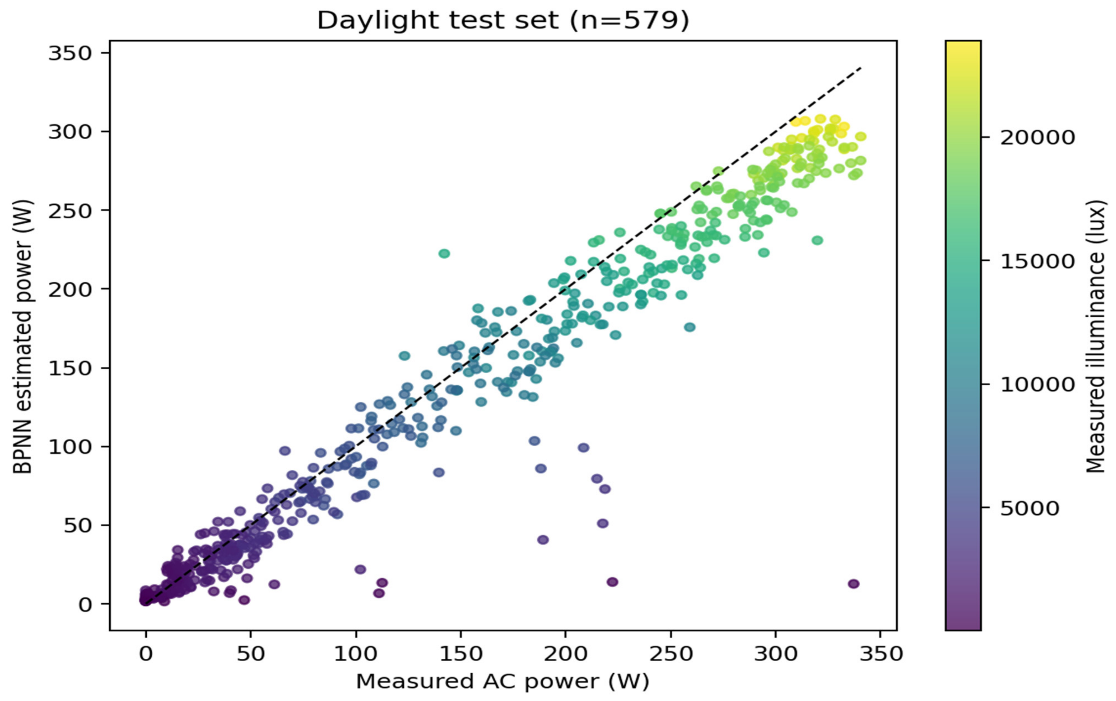
To further examine model performance under daylight conditions, Figure 8 presents a comparison between measured and BPNN-estimated AC power for 579 daylight observations. The data points are colored according to measured illuminance to illustrate the relationship between prediction performance and illumination conditions.

Figure 8. Daylight-only measured versus BPNN-estimated AC power, with each point colored by measured illuminance (lux; n = 579). The dashed line represents the 1:1 reference line (y = x), indicating perfect agreement between measured and estimated power.

4.3. Optional Nighttime Post-Processing

For BPNN, fixed-night post-processing changed all-hours MSE only from 531.95 to 529.89 W² and MAE from 11.11 to 10.23 W, while R² remained 0.95 at two-decimal precision. Thus, the principal performance result does not depend on nighttime clamping. The PV-active and fixed-night performance metrics are summarized in Table 11.

Table 11. PV-active and fixed-night performance metrics across evaluated models.

Model	PV-Active MSE	PV-Active MAE	PV-Active R2	Fixed-Night MSE	MAE	R2
Persistence	4959.02	52.89	0.60	2456.49	25.96	0.79
Linear Regression	2203.11	34.51	0.82	1096.67	17.24	0.90
XGBoost	1721.55	29.02	0.86	855.79	14.39	0.93
BPNN	1065.63	20.58	0.91	529.89	10.23	0.95

4.4. Residual Characteristics

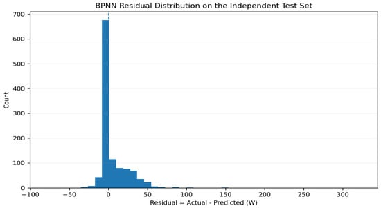
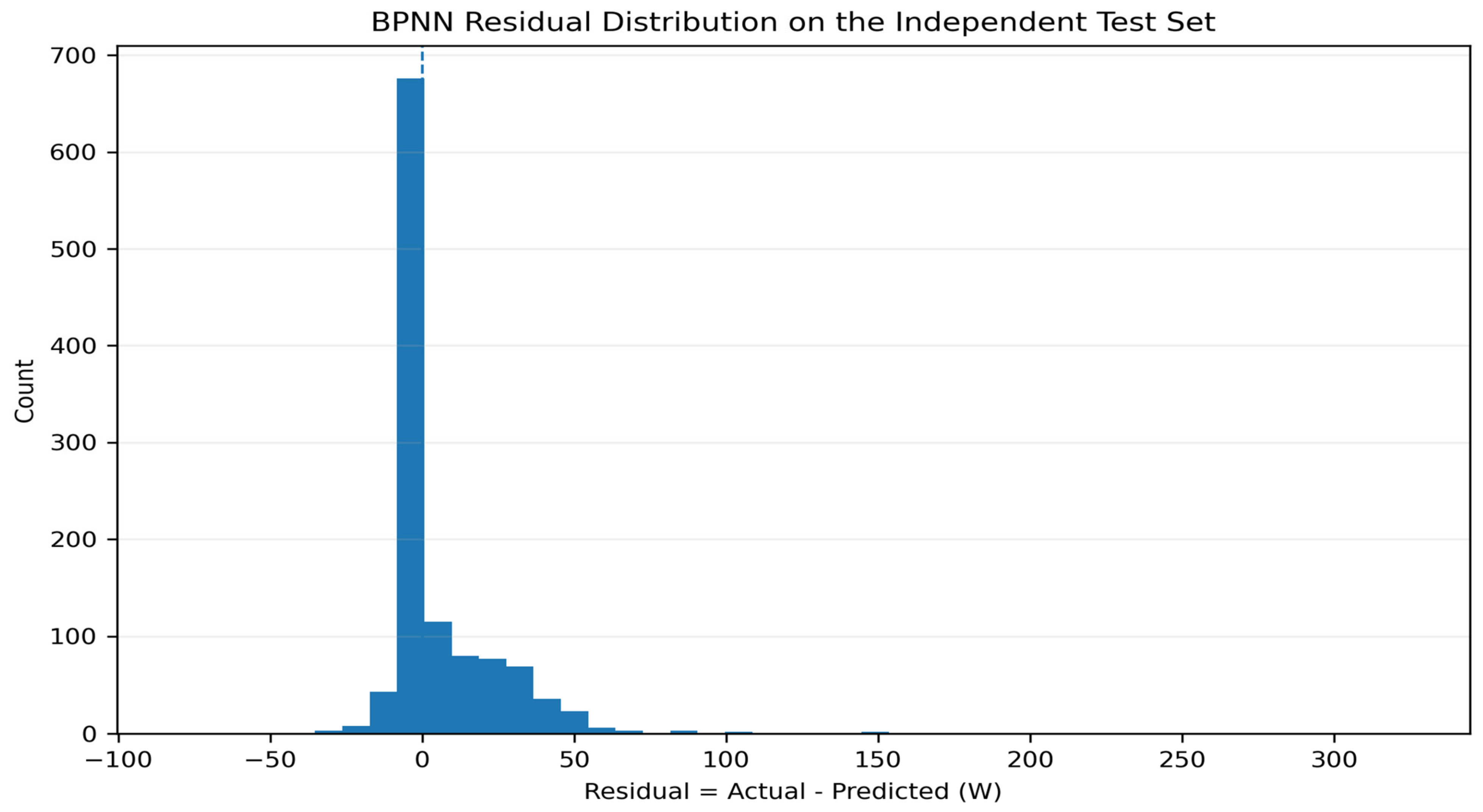
Residuals were defined as Actual − Predicted. For the BPNN test set, the mean residual was 7.41 W, median −1.28 W, standard deviation 21.85 W, skewness 5.08, and kurtosis 51.35. Most residuals were concentrated near zero, but a pronounced positive tail indicates occasional substantial underestimation events. The residuals are therefore not described as Gaussian or homoscedastic. The residual distribution is shown in Figure 9.

Figure 9. Historical single-run BPNN residual distribution on the original held-out test set (secondary analysis).

4.5. Architecture Sensitivity

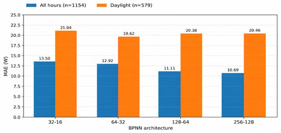
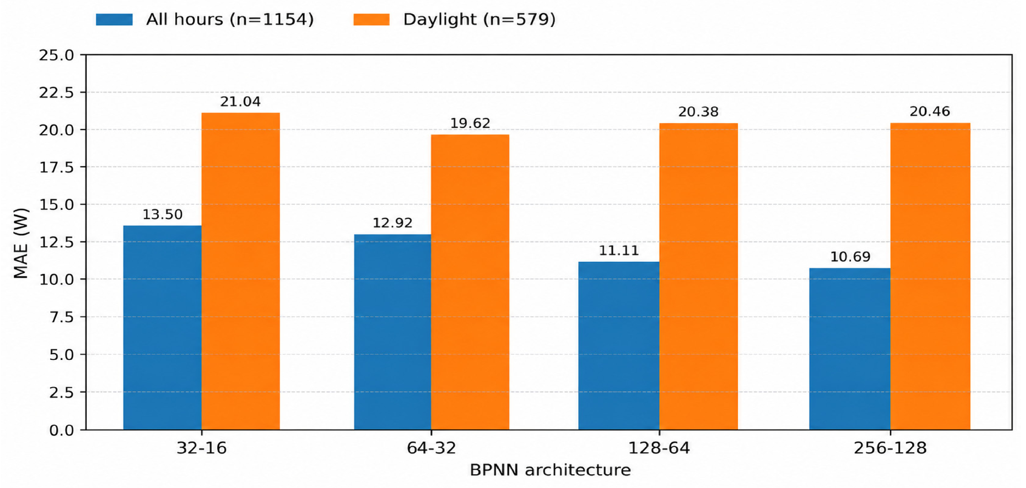
The 128–64 architecture was the predefined primary configuration. The other tested architectures (32–16, 64–32, and 256–128) were examined to assess architectural sensitivity, not to select the primary model based on held-out test outcomes. The architecture sensitivity results are summarized in Table 12. Differences across the architectures were modest, and the 128–64 model is not claimed to be universally optimal. The architecture-specific MAE comparison is illustrated in Figure 10.

Table 12. BPNN architecture sensitivity under identical chronological split and preprocessing conditions.

Architecture	Best Epoch	All-Hours MSE	MAE	R2	Daylight MSE	MAE	R2
32–16	33	561.11	13.50	0.95	1079.12	21.04	0.91
64–32	39	542.10	12.92	0.95	1001.75	19.62	0.92
128–64	21	531.95	11.11	0.95	1056.13	20.38	0.92
256–128	29	547.37	10.69	0.95	1089.77	20.46	0.91

Figure 10. Historical single-run architecture sensitivity for the same original held-out test observations (secondary analysis). Bars show MAE (W), with numerical values annotated; all-hours n = 1154 and daylight n = 579 for each architecture.

4.6. Temporal Robustness

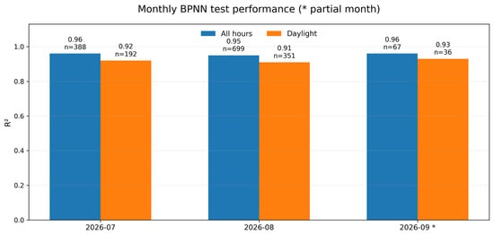
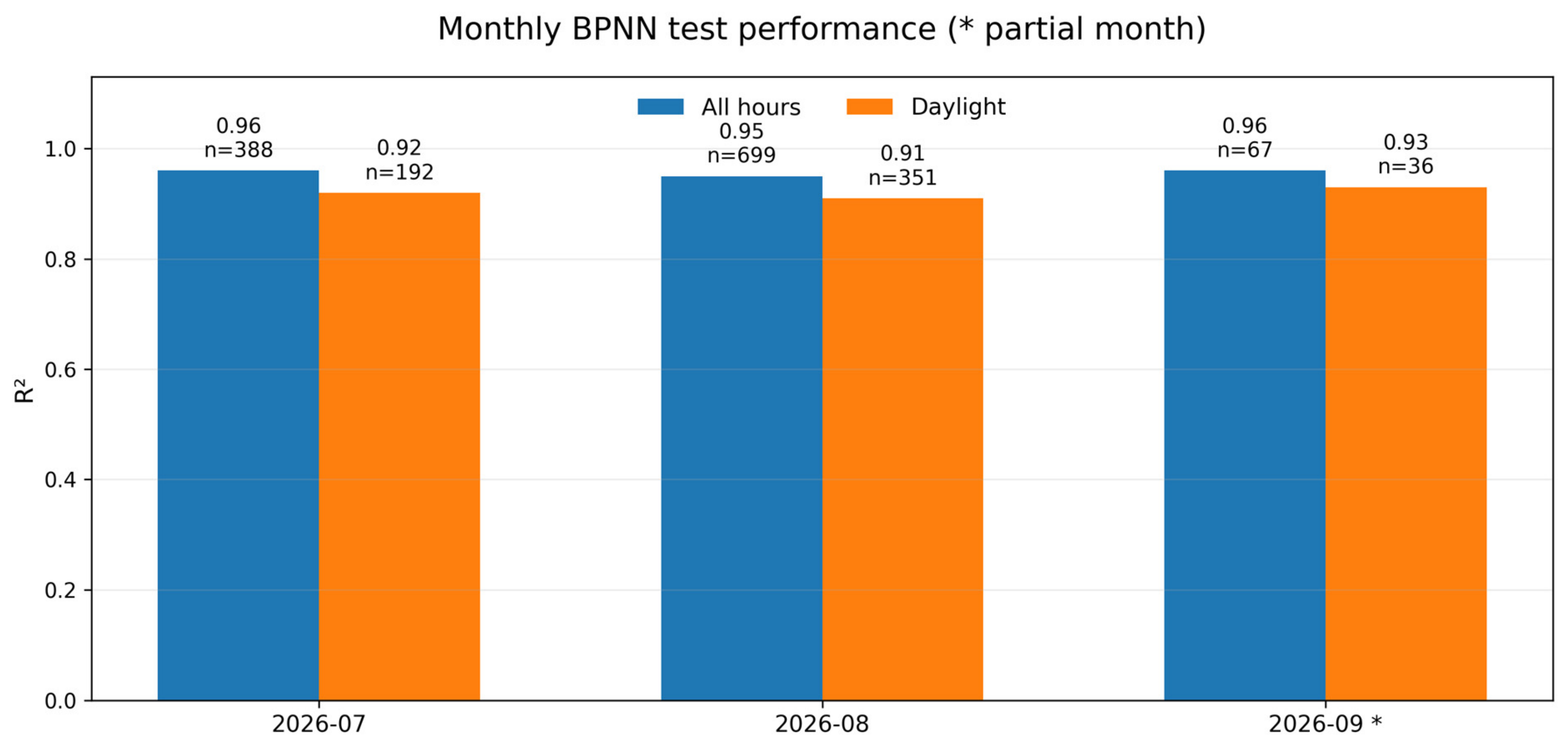
The original single-run BPNN monthly test-period evaluation provides an additional temporal check. July, August, and the partial September test segment retained similar BPNN performance, although September contains substantially fewer observations and should not be interpreted as a full-month estimate. The monthly BPNN performance comparison is shown in Figure 11.

Figure 11. Historical single-run BPNN monthly R² for all-hours and daylight test observations (secondary analysis). Each bar displays R² and its sample size (n); September 2026 is a partial month.

Multi-seed statistical reporting: BPNN feature ablation and XGBoost repeated-training results are means ± sample standard deviations over ten seeds (40–49), using the same exported processed hourly CSV, fixed chronological train/validation/test partition (3692/924/1154), and training-only preprocessing. Five-input XGBoost used at most 1000 estimators, learning rate 0.03, maximum depth 4, minimum child weight 1, row/column subsampling of 0.9, and early stopping patience 50; its all-hours MAE was 14.59 ± 0.14 W in the reproducible paired retraining export. Three-input XGBoost achieved 14.80 ± 0.20 W on the same held-out hours. The original single-run XGBoost MAE of 14.53 W is retained separately. Exact metrics may differ across earlier supplementary exports; the matched multi-seed paired comparisons here are calculated only from retrained_test_predictions.csv (raw cohort), with dataset, model, seed, timestamp, actual, and predicted fields.

4.7. Multi-Seed Robustness and Feature Ablation

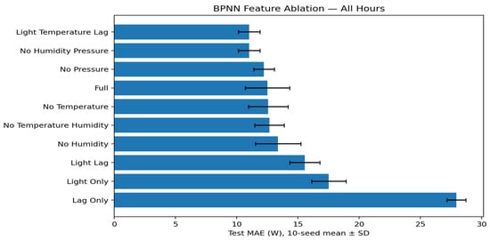
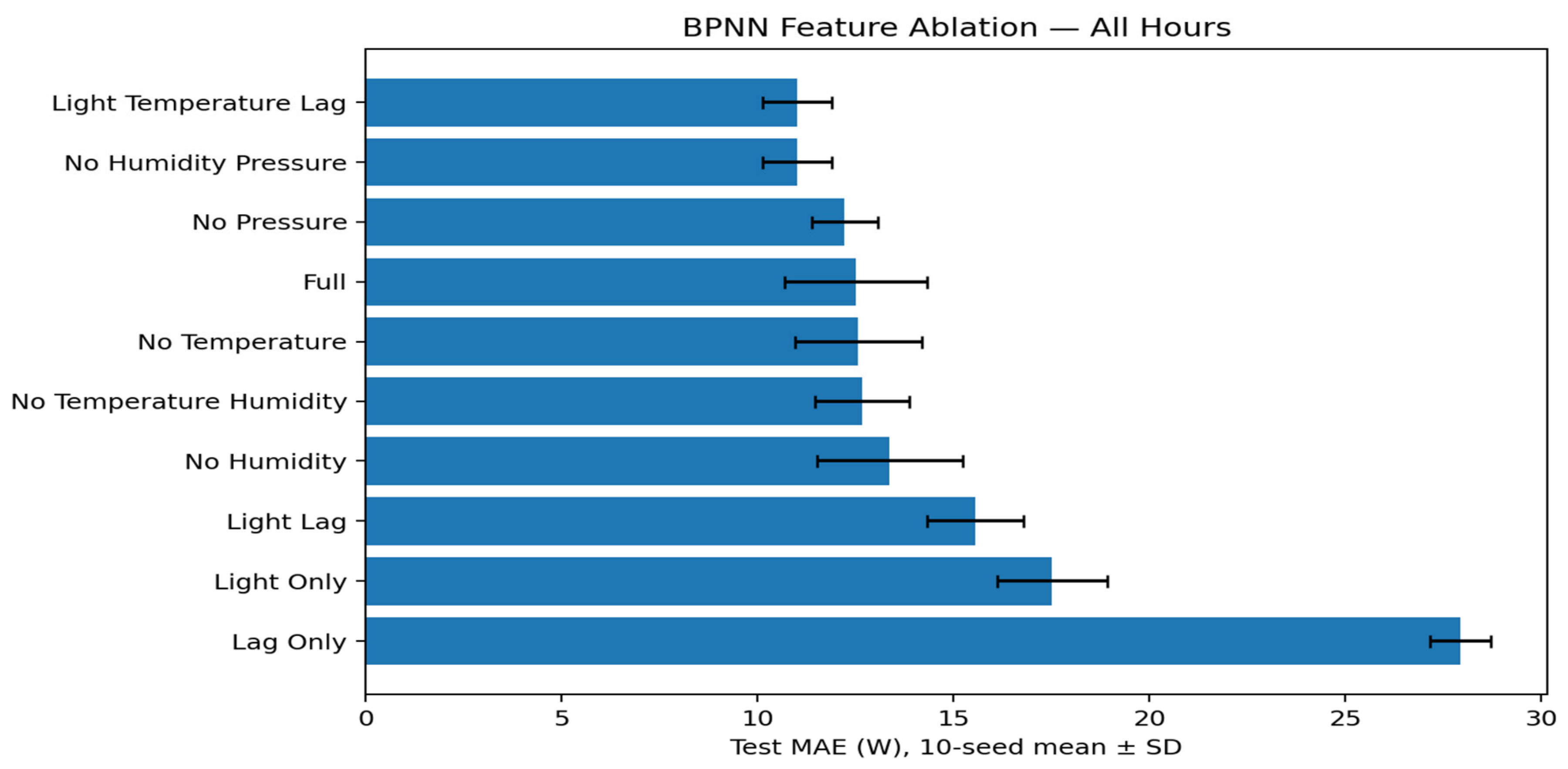
Across ten random seeds, the full five-feature BPNN achieved all-hours MSE 591.03 ± 80.96 W², MAE 12.52 ± 1.82 W, and R² 0.9484 ± 0.0071 (mean ± sample SD). The reduced illuminance, ambient-temperature, and previous-hour-power configuration achieved MSE 512.10 ± 45.39 W², MAE 11.02 ± 0.88 W, and R² 0.9553 ± 0.0040. Daylight MAE was 19.49 ± 1.55 W for the reduced configuration versus 21.70 ± 2.52 W for the full configuration. The No-Humidity/Pressure and Light/Temperature/Lag configurations are the same three-feature set, not independent experiments. These findings suggest potential input simplification at this site, without demonstrating universal redundancy of humidity or pressure. The three-input configuration was identified through the reported feature-ablation results on the held-out test period; therefore, this configuration choice is exploratory and test-informed rather than an independently validated feature-selection result. The same test period should not be treated as independent confirmation of the selected feature set. Prospective confirmation on a new independent period is required. The ten-seed feature-ablation MAE results are illustrated in Figure 12.

Figure 12. All-hours MAE across ten random seeds for feature-ablation configurations (error bars indicate standard deviation).

4.8. Interpretable Empirical Baseline

An interpretable illuminance–temperature empirical baseline was evaluated to provide a simpler reference for assessing the contribution of the BPNN model. The baseline uses measured illuminance and ambient temperature as explanatory variables. Because BH1750 measurements represent illuminance (lux) rather than calibrated solar irradiance (W/m²), this approach is described as an empirical baseline rather than a physically calibrated PV power model.

The empirical baseline was fitted by ordinary least squares using scikit-learn LinearRegression with an intercept and two terms derived from the adjusted illuminance proxy L(t) = solarradiation_adj and ambient temperature T(t) = tempc (°C). Its test-time prediction was $\hat{\mathrm{P}}$(t) = max{0, 0.3675751819 + 0.5863096079 L(t) + 0.0120142128 L(t)[T(t) − 25]}. The 25 °C reference was used to construct the interaction term. Coefficients were estimated exclusively from the first 3692 chronologically ordered training observations in the original V9.2 processed hourly dataset (5770 observations overall); the 924 validation and 1154 test observations were not used for fitting. Negative predictions were clipped to zero, without an additional clock-based nighttime zeroing rule. On the original 1154 h held-out test partition, the empirical baseline achieved MAE 15.02 W, RMSE 29.65 W, and R² 0.9232; for the daylight subset (06:00–17:59; n = 579), MAE was 29.30 W. The primary three-input BPNN achieved all-hours MAE 11.02 ± 0.88 W over ten seeds on the same original test partition. This is an empirical statistical comparator, not a calibrated PV physical model.

However, the comparison should not be interpreted as isolating the effect of nonlinear modeling alone, because the reduced BPNN also includes previous-hour measured power as an additional input. Furthermore, the empirical baseline does not establish the accuracy of a calibrated irradiance-based physical model.

4.9. Additional Evidence: Feature Ablation and Illuminance-Dependent Error

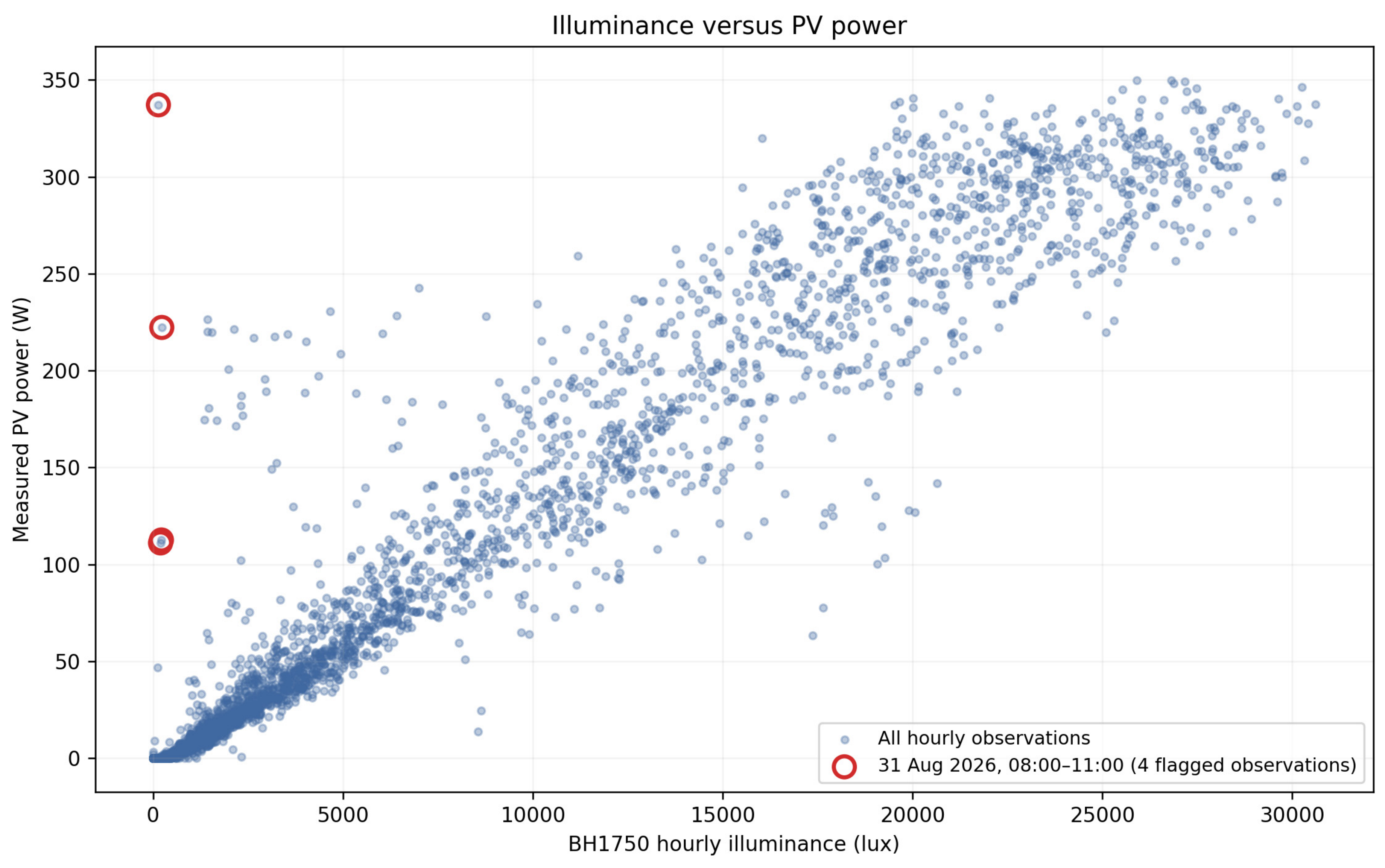
Data-quality audit: Four hourly observations on 31 August 2026 (08:00–11:00) showed BH1750 illuminance of 137.8–226.8 lux despite measured PV power of 111.1–337.1 W. Five-minute records show illuminance rising from 100 lux at 12:00 to 17,031 lux at 12:05 and remaining substantially higher thereafter. This supports a temporary illuminance measurement/acquisition anomaly followed by recovery; a device restart cannot be verified from these measurements alone. The four observations were flagged for interpretation but retained in the original modeling data. Primary model metrics retain these observations; separate post hoc excluded-observation metrics are now reported below. The original raw-series audit also flagged 242 daytime zero-lux records across 82 h; these are distinct from the four low-but-nonzero illuminance/high-power observations. The ten-seed BPNN feature-ablation results are summarized in Table 13.

Table 13. Ten-seed all-hours BPNN feature ablation (same chronological test set; mean ± SD). The No Humidity/Pressure and Light + Temperature + Lag configurations contain identical features and are not independent comparisons.

Feature Configuration	MAE (W)	SD (W)	R2
Light Temperature Lag	11.02	0.88	0.9553
No Humidity Pressure	11.02	0.88	0.9553
No Pressure	12.23	0.85	0.9520
Full	12.52	1.82	0.9484
No Temperature	12.57	1.62	0.9446
No Temperature Humidity	12.67	1.21	0.9490
No Humidity	13.38	1.85	0.9452
Light Lag	15.57	1.24	0.9250
Light Only	17.53	1.40	0.9096
Lag Only	27.96	0.77	0.8001

Five-minute zero-illuminance verification (supplementary audit): In the date-filtered 1 January 2026 00:00–3 September 2026 18:00 weather and inverter exports, all 242 records previously identified using the fixed 06:00–17:59 daytime screening window were matched to inverter records by recorded timestamp. Of these, 202 occurred at 06:00–07:59 and 40 at 16:00–17:59; none occurred at 08:00–15:59. The maximum contemporaneously matched inverter power was 1.2 W. The 242 records spanned 82 distinct clock hours, none in the original test partition; three records belonged to one hour already excluded by the retrospective sample-count QC (21 February 2026 17:00, four valid lux samples). Therefore, zero lux alone was not treated as a sensor-fault label or an automatic exclusion rule. These zero-valued five-minute records are distinct from the four 31 August 2026 low-but-nonzero illuminance/high-power hourly anomalies (08:00–11:00). This is a fixed-clock daytime screen, not an astronomical sunrise/sunset classification, and the matched power values are instrument readings rather than proof of true zero production.

The three-input BPNN (illuminance, temperature, and preceding-hour PV power) is the recommended prediction configuration (ten-seed MAE 11.02 ± 0.88 W); the five-input BPNN (12.52 ± 1.82 W) is retained as a feature-ablation baseline. Matched-feature ten-seed comparisons use three-input XGBoost (14.80 ± 0.20 W) for the primary comparison and five-input XGBoost (14.59 ± 0.14 W) for the five-input sensitivity analysis. Different input sets must not be described as like-for-like comparisons.

Quality-controlled retraining sensitivity (10 seeds, separate from the fixed-prediction four-hour exclusion above): Table 14 reports the four model/input combinations. Native-test results evaluate the raw-trained models on 1154 observations and cleaned-trained models on 1145 observations; changes in these metrics combine altered training and altered test composition. To isolate the retraining comparison more fairly, both models were additionally evaluated on the identical 1145 quality-controlled test timestamps (common-clean-test). On this common set, BPNN_3 MAE increased slightly after retraining (10.34 to 10.46 W), whereas BPNN_5 and both XGBoost configurations changed only modestly. Thus, quality-control exclusions materially change the native-test summary but do not consistently improve retrained-model accuracy on matched test cases. These comparisons are descriptive and do not establish statistical significance.

Table 14. Supplementary quality-controlled retraining sensitivity: ten-seed mean all-hours MAE; native raw n = 1154, native cleaned n = 1145, and matched common-clean-test n = 1145 for both training conditions. Δ = cleaned-trained minus raw-trained MAE on the matched test set (negative favors cleaning).

Model	Raw Native MAE (W)	Cleaned Native MAE (W)	Raw Common MAE (W)	Cleaned Common MAE (W)	Common Δ (W)
BPNN_3	11.02	10.46	10.34	10.46	+0.11
BPNN_5	12.52	11.79	11.81	11.79	−0.02
XGBoost_3	14.80	13.93	14.07	13.93	−0.14
XGBoost_5	14.59	13.86	13.88	13.86	−0.02

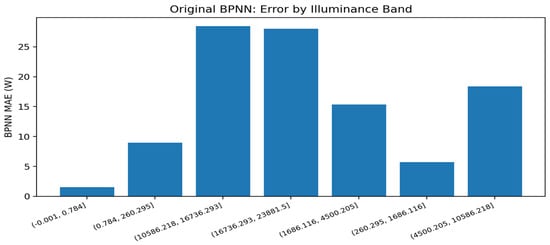
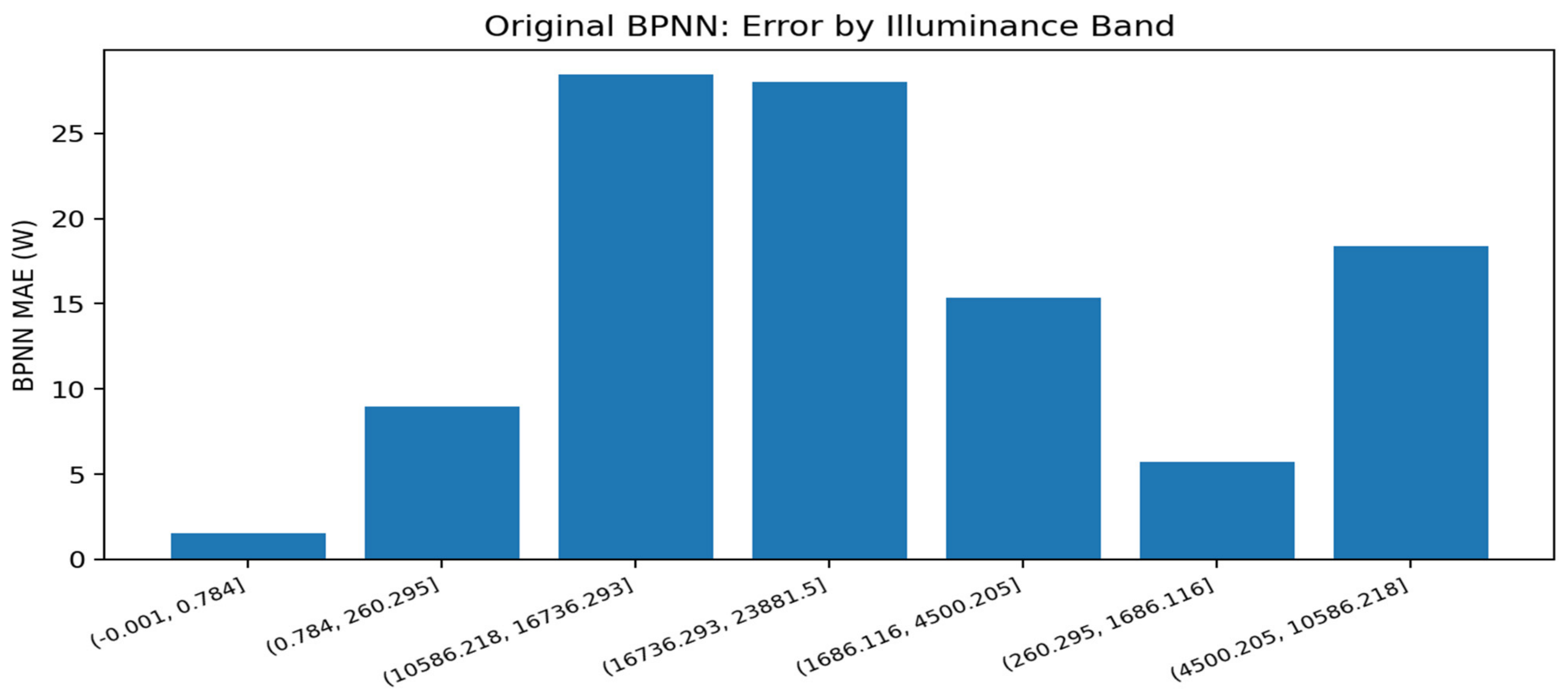
Post hoc anomaly-exclusion sensitivity (fixed predictions; no retraining): Four flagged observations from 31 August 2026 (08:00–11:00) were excluded only when computing supplementary test metrics. For ten-seed BPNN, mean ± sample SD MAE decreased from 11.02 ± 0.88 to 10.40 ± 0.88 W for three inputs, and from 12.52 ± 1.82 to 11.92 ± 1.83 W for five inputs. For ten-seed five-input XGBoost, it decreased from 14.59 ± 0.12 to 14.00 ± 0.12 W. In the separate original single-run comparisons, BPNN MAE decreased from 11.11 to 10.51 W and XGBoost MAE from 14.53 to 13.93 W. Raw and excluded metrics use the same fixed predictions within each experiment (n = 1154 and 1150, respectively). The four flagged observations remain in the primary results. The original BPNN prediction errors grouped by measured illuminance are shown in Figure 13. This post hoc test-set exclusion does not implement invalid-data filtering before chronological splitting and does not represent retraining on cleaned data. The four-observation anomaly-exclusion sensitivity results are summarized in Table 15.

Figure 13. Original BPNN test error grouped by measured illuminance. Bins are defined by the analysis output and reflect uneven day/night sample densities.

Table 15. Post hoc four-observation anomaly-exclusion sensitivity (fixed predictions without retraining; raw test n = 1154, excluded test n = 1150).

Model/Experiment	Raw MAE (W)	Four Excluded MAE (W)
BPNN, 3-input (10 seeds)	11.02 ± 0.88	10.40 ± 0.88
BPNN, 5-input (10 seeds)	12.52 ± 1.82	11.92 ± 1.83
XGBoost, 5-input (10 seeds)	14.59 ± 0.14	14.00 ± 0.12
BPNN, original single run	11.11	10.51
XGBoost, original single run	14.53	13.93

Supplementary sensitivity table. Raw n = 1154; after excluding the same four flagged test hours n = 1150. Ten-seed values are mean ± sample SD. The original single-run models are separate experiments and must not be pooled with ten-seed estimates.

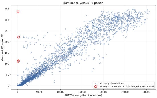
The relationship between measured illuminance and AC power, including the four flagged observations, is illustrated in Figure 14.

Figure 14. Relationship between hourly BH1750 illuminance (lux) and measured AC power (W) during field operation. Red outlined circles identify four anomalously low-illuminance/high-power observations recorded on 31 August 2026 at 08:00–11:00 (137.8–226.8 lux; 111.1–337.1 W). These points were retained in the modeling data and are discussed in the data-quality audit.

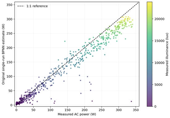
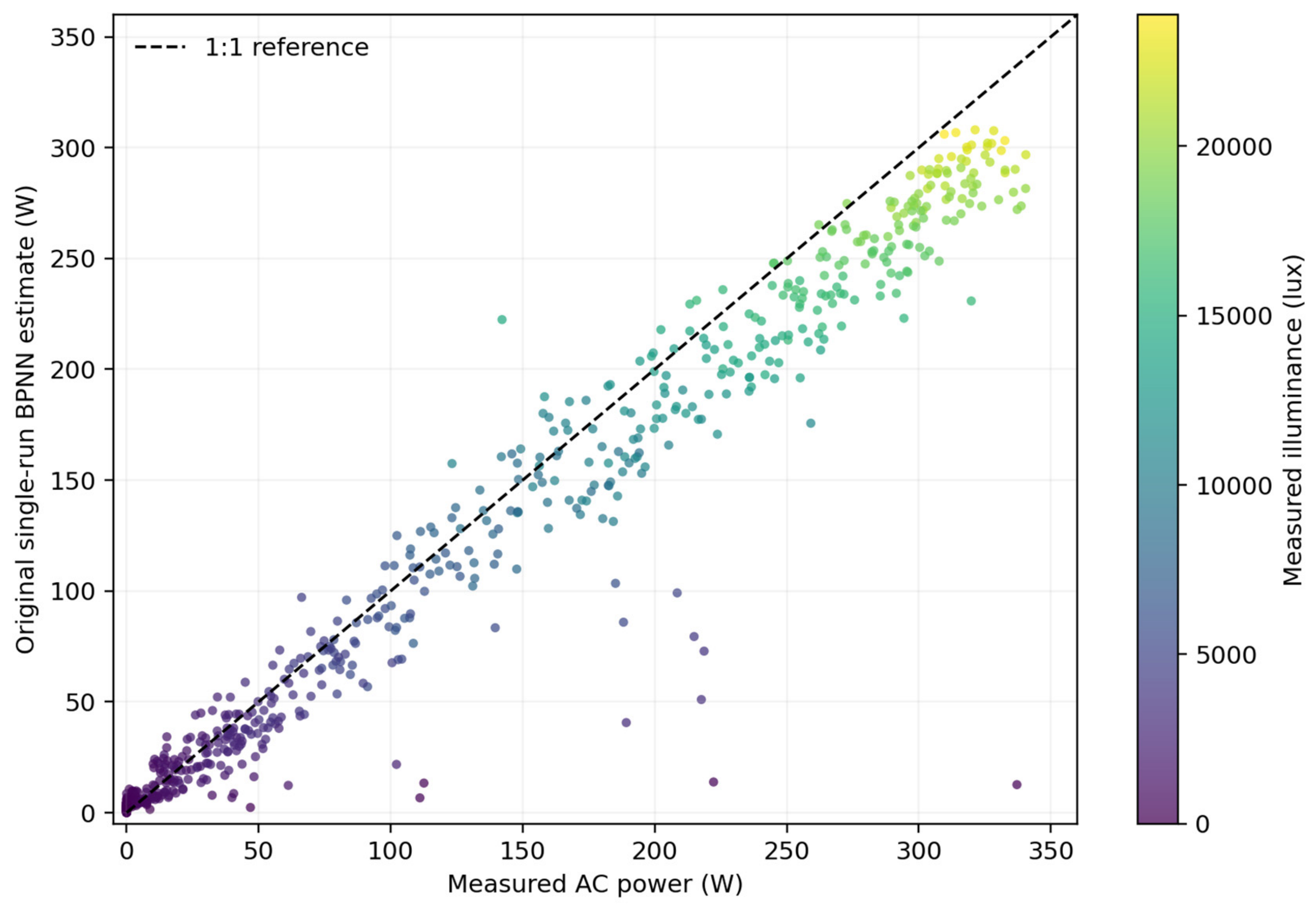
The relationship between measured and BPNN-estimated AC power on the original held-out test set is illustrated in Figure 15.

Figure 15. BPNN-estimated versus measured target AC power on the original held-out test set (n = 1154), with points colored by measured illuminance (lux).

Additional high-output diagnostic using the original paired test predictions (02_paired_predictions.csv; target_power and pred_bpnn, without fixed-clamp post-processing): 149 of 1154 held-out hours had target power > 250 W (12.9%). In this group, BPNN MAE was 33.13 W, mean signed error (prediction minus target) was −33.06 W, and 147/149 (98.7%) predictions underestimated the target. The two high-output bands in Table 16 contain 85 observations in (250, 300] W and 64 above 300 W, totaling 149. These original single-run diagnostics are distinct from the ten-seed QC-cleaned analysis in Table 17. The latter provides an independently traceable training–test power-distribution comparison; neither analysis establishes a causal mechanism for the underestimation.

Table 16. Power-stratified MAE and bias on the identical original experimental test observations.

Actual-Power Band	n	BPNN MAE (W)	XGBoost MAE (W)	BPNN Bias (W)	XGBoost Bias (W)
0 W	569	1.68	0.16	1.68	0.16
(0, 50] W	189	6.69	7.19	−1.47	−6.54
(50, 120] W	97	15.00	18.04	−10.35	−12.41
(120, 250] W	150	28.05	41.44	−21.98	−40.09
(250, 300] W	85	29.71	46.89	−29.59	−46.89
>300 W	64	37.67	52.59	−37.67	−52.59

Table 17. Training-range coverage and power-stratified errors for the QC-cleaned three-input BPNN (10 seeds). Categories overlap and should not be summed; the original uncleaned test results remain in Table 16.

QC-Cleaned Test Category	n	BPNN_3 MAE ± SD (W)	Bias (W)
Within training target-power range (0–349.92 W)	1145	10.46 ± 0.85	−5.43
Above training target-power maximum	0	N/A	N/A
≤250 W	998	7.69 ± 0.88	−1.95
>250 W	147	29.24 ± 3.83	−29.05
>300 W	63	30.20 ± 3.85	−30.08

The plots and Table 13 were reconstructed from previously generated experiment outputs. The multi-seed feature-ablation runs used the rounded exported hourly CSV, whereas the original single-seed evaluation used unrounded in-memory aggregates; the two experiments are therefore reported separately rather than as identical seed-42 replications. The BH1750 raw-data audit found 68,990 records and no values above 60,000 lux, but this screening threshold does not establish the device’s configured saturation limit.

4.10. Error Stratification by Measured Target PV Power

The original experimental paired predictions were grouped by target AC power (target_power), using un-clamped pred_bpnn and pred_xgboost. XGBoost was more accurate in the 0 W band (MAE 0.16 W vs. 1.68 W for BPNN), whereas BPNN had lower MAE in each of the five nonzero bands. At >300 W, MAE was 37.67 W for BPNN and 52.59 W for XGBoost, and both models showed negative prediction bias. The 0 W band has constant ground truth; R² is mathematically undefined and is therefore not reported. Band-specific differences are descriptive and were not separately tested for significance.

4.11. Training–Test Power Coverage and High-Power Error (QC-Cleaned Multi-Seed Analysis)

To assess whether high-power underestimation reflected extrapolation beyond the training target-power range, the original 5770 model-ready hourly records were aligned one-to-one by timestamp with the presplit Round 2 quality audit. After exclusion of 35 hourly observations (23 training, 3 validation, and 9 test), the fixed chronological cohorts contained 3669 training, 921 validation, and 1145 test hours. The split labels “validation” and “val” were normalized without changing cohort membership. The training target-power maximum was 349.92 W, compared with 340.50 W in testing; therefore all 1145 QC-cleaned test hours fell within the observed training target-power range, with zero observations beyond it. An out-of-range test error cannot be estimated because no such test hours occurred.

High-power observations were nonetheless less frequent in training: 330/3669 (8.99%) training hours versus 147/1145 (12.84%) test hours exceeded 250 W. The training and test target-power P95 values were 286.64 and 302.16 W, respectively (P99: 325.01 and 328.02 W). Training, validation, and test maxima were 349.92, 349.75, and 340.50 W. For the QC-cleaned three-input BPNN, the ten-seed test MAE was 7.69 ± 0.88 W at ≤250 W (n = 998), compared with 29.24 ± 3.83 W at >250 W (n = 147); the respective mean signed biases were −1.95 and −29.05 W. The >300 W group (n = 63) had MAE 30.20 ± 3.85 W and bias −30.08 W. All-hours MAE was 10.46 ± 0.85 W and bias −5.43 W (n = 1145). The ± values are the sample SD across ten seeds; signed bias is prediction minus target.

5. Discussion

The results should be interpreted as a field-system evaluation rather than a claim of a new machine-learning algorithm. Prior PV studies have established the usefulness of artificial intelligence and data-driven modeling [1,2,3], while recent IoT-oriented work demonstrates the feasibility of low-cost sensing and monitoring architectures [6,7,8]. The present study combines these strands with an explicit gap audit, exact-lag construction, chronological validation, and multiple baselines in one reproducible workflow.

The supplementary quality-controlled retraining experiment distinguishes the effect of excluding low-quality test observations from the effect of refitting models. Although native-test MAE was lower after cleaning for all four configurations, the matched-test changes were small and mixed. In particular, BPNN_3 slightly worsened on identical cleaned test hours. This limits any claim that quality filtering alone improves generalization; the original unfiltered results remain the primary benchmark.

Cost and comparison scope: The approximately USD 31.50 estimated component BOM covers the prototype sensing/acquisition subsystem, not total installed lifecycle cost (e.g., enclosure, installation, networking and maintenance). Local measurements were collected at the PV test site, but this does not establish greater accuracy or cost-effectiveness than free public meteorological datasets. No matched public-weather-data baseline or multisite evaluation was conducted. The contribution is field feasibility under the investigated conditions, not universal superiority.

The comparison against persistence is particularly important because preceding-hour PV power is included as an input feature. The improvement over persistence indicates that contemporaneous micro-meteorological measurements and nonlinear mapping provide information beyond simply reusing the previous hour’s generation. XGBoost further strengthens this comparison by providing a nonlinear tree-based benchmark rather than limiting the analysis to linear and autoregressive baselines. Although the entire QC-cleaned test target-power range was covered by the training observations, this does not establish that all combinations of illuminance, temperature, and lagged power were represented. The higher test frequency of >250 W observations and possible seasonal covariate changes may contribute to the high-power negative bias, but these are not proven causes. The 250 W cutoff is a diagnostic grouping threshold, not a validated universal reliability boundary.

The daylight-only and PV-active analyses address a common concern in PV model evaluation: all-hours datasets contain many zero or near-zero nighttime observations that can make aggregate metrics appear artificially favorable. In the original single-run BPNN evaluation (secondary historical analysis), R² values were 0.92 for daylight and 0.91 for PV-active observations, while the optional fixed-night rule changed the all-hours MSE only marginally. These single-run metrics are supplementary and do not replace the primary ten-seed, three-input BPNN–XGBoost comparison.

The BPNN itself is an established model and is not claimed as an algorithmic innovation. The engineering contribution is the integration of localized low-cost sensing, field acquisition, gap-aware data construction, chronological validation, and comparative modeling in a single auditable workflow. This positioning is consistent with the practical IoT/PV monitoring literature [6,7,8] while addressing a different estimation objective.

In comparison with recent studies [9,10,11,12,13,14,15], the principal contribution is an auditable field evaluation of a low-cost multi-sensor system for expected hourly PV AC power, not a new sensor calibration method, an embedded ANN irradiance meter, or an experimentally verified fault-diagnosis system. Direct numerical rankings across these studies would be misleading because they estimate different targets (irradiance, AC power, or fault class), use different scales, and adopt different reference instruments. The absence of pyranometer calibration, multi-site transfer testing, and labeled fault validation remains a material limitation.

Several limitations remain. The study uses a single 545 W installation and an observation period shorter than a complete annual cycle. The BH1750 quantity is an illuminance-derived solar-input proxy rather than calibrated pyranometer irradiance. External multi-site validation was not performed. Although the architecture is compatible with local computation, the present study does not experimentally benchmark embedded inference latency, memory use, or energy consumption; therefore, proven edge deployment, scalability, predictive maintenance, and fault-detection capabilities are not claimed. Field data availability was also occasionally affected by power interruptions, acquisition-node or collector resets, and communication failures. These intervals were explicitly excluded rather than reconstructed, preserving evaluation integrity at the cost of reduced temporal coverage. The AHT10 temperature and humidity sensor had no radiation shield during the field campaign, and solar-heating effects were not independently quantified. Future work will install a suitable ventilated radiation shield and compare shielded versus unshielded temperature measurements and their influence on PV power estimation accuracy.

The primary matched-feature, ten-seed BPNN–XGBoost comparison favors the three-input BPNN (mean seed-level paired MAE gain 3.79 ± 0.96 W; hierarchical moving-block bootstrap 95% interval 2.90–4.63 W). The supplementary seed-level Wilcoxon test and hierarchical bootstrap share the same fixed site and test period and should not be interpreted as evidence of independent multi-site or multi-season replication. The original single-run paired interval of 2.67–4.24 W is preserved only as a historical secondary analysis. The power-band audit shows increasing high-output underprediction, limiting generalizability and motivating independent validation.

The study-period BH1750 series contained 68,990 valid illuminance records, a maximum of 37,450 lux, and no values exceeding the 60,000-lux screening threshold. No negative values or duplicate timestamps were observed; 32 sampling gaps longer than 10 min and 242 daytime zero-lux records were flagged. Selected large underestimation residuals coincided with unexpectedly low optical measurements. Subsequent field-data review identified acquisition errors affecting some observations, which are discussed as data-quality limitations rather than proof of sensor saturation or a specific hardware fault. The absence of high-range readings does not rule out saturation under every BH1750 configuration. Original test observations were retained; no high-error points were removed post hoc.

The targeted five-minute cross-source check found no zero-lux record in the 08:00–15:59 screening band or with matched inverter power above 1.2 W. Consequently, the reviewer-noted approximately 100–340 W/near-zero-illuminance points in Figure 14 should not be conflated with the 242 exactly-zero five-minute readings: the four flagged 31 August observations had low but nonzero hourly mean illuminance (137.8–226.8 lux). The 35 h retrospective exclusion and ten-seed retraining comparison in Table 14 are unchanged by this descriptive zero-lux audit. The date-filtered export and the separately defined original model-ready cohort must not be treated as having identical denominators without a full pipeline reconciliation. All 1145 QC-cleaned test targets were within the training target-power range (0–349.92 W), but high-power conditions (>250 W) were less frequent in training (8.99%) than testing (12.84%). The QC-cleaned three-input BPNN had a ten-seed MAE 29.24 ± 3.83 W above 250 W versus 7.69 ± 0.88 W at or below 250 W. Accordingly, coverage of the target-power range does not establish uniformly reliable predictions; these results are specific to the evaluated site and period.

6. Conclusions

This study designed and field-evaluated a low-cost sensing and machine-learning workflow for hourly PV AC power estimation. Of 5899 candidate hourly timestamps, 5770 model-ready observations were retained after completeness screening and exact one-hour lag construction. The recommended three-input BPNN achieved ten-seed all-hours MAE 11.02 ± 0.88 W (mean ± sample SD) on the fixed independent chronological test period, compared with 14.80 ± 0.20 W for matched three-input XGBoost. The ten-seed paired improvement was 3.79 ± 0.96 W with a hierarchical moving-block bootstrap 95% interval of 2.90–4.63 W, conditional on the single-site test series. The original single-run BPNN MAE of 11.11 W and its four-model comparison remain historical secondary results rather than the principal performance claim. Future work should extend to multiple sites and seasons, calibrated irradiance measurements, and measured embedded inference costs.

Feature ablation showed that adding humidity and pressure to the illuminance–temperature–previous-hour-power model increased ten-seed mean MAE from 11.02 ± 0.88 to 12.52 ± 1.82 W at this site. The five-input model is therefore retained for sensitivity analysis rather than recommended deployment. An interpretable illuminance–temperature empirical baseline achieved MAE 15.02 W in its separate experiment. The expected-power reference may complement measured PZEM-004T output, but fault-detection accuracy, calibrated irradiance sensing, on-device computation, and broader operating-range validity were not established. In the separate QC-cleaned ten-seed analysis, MAE was 29.24 ± 3.83 W for test hours above 250 W versus 7.69 ± 0.88 W at or below 250 W. The 250 W cutoff is a diagnostic grouping threshold, not a validated reliability boundary. The 242 five-minute zero-lux readings are screening observations and must not be equated with the four distinct low-but-nonzero illuminance/high-power anomalies.

7. Software Environment and Reproducibility

All model training, feature-ablation experiments, statistical analyses, and evaluation procedures were conducted in the same software environment: Fedora Linux 44 (Forty Four) with Python 3.14.7. The principal software libraries were NumPy 2.5.2, pandas 3.0.5, PyTorch 2.14.0, scikit-learn 1.9.0, SciPy 1.18.1, and XGBoost 3.4.1. PyTorch was used for BPNN training, scikit-learn for feature scaling, empirical regression, and model evaluation, and SciPy for statistical testing. The software environment was maintained consistently across the reported experiments.

References

- Antonanzas, J.; Osorio, N.; Escobar, R.; Urraca, R.; Martinez-de-Pison, F.J.; Antonanzas-Torres, F. Review of photovoltaic power forecasting. Sol. Energy 2016, 136, 78–111. [Google Scholar] [CrossRef] [Scilit]
- Mellit, A.; Kalogirou, S.A. Artificial intelligence techniques for photovoltaic applications: A review. Prog. Energy Combust. Sci. 2008, 34, 574–632. [Google Scholar] [CrossRef] [Scilit]
- Voyant, C.; Notton, G.; Kalogirou, S.; Nivet, M.-L.; Paoli, C.; Motte, F.; Fouilloy, A. Machine learning methods for solar radiation forecasting: A review. Renew. Energy 2017, 105, 569–582. [Google Scholar] [CrossRef] [Scilit]
- Tercha, W.; Tadjer, S.A.; Chekired, F.; Canale, L. Machine Learning-Based Forecasting of Temperature and Solar Irradiance for Photovoltaic Systems. Energies 2024, 17, 1124. [Google Scholar] [CrossRef] [Scilit]
- Matos, M.; Almeida, J.; Gonçalves, P.; Baldo, F.; Braz, F.J.; Bartolomeu, P.C. A Machine Learning-Based Electricity Consumption Forecast and Management System for Renewable Energy Communities. Energies 2024, 17, 630. [Google Scholar] [CrossRef] [Scilit]
- Hamied, A.; Mellit, A.; Benghanem, M.; Boubaker, S. IoT-Based Low-Cost Photovoltaic Monitoring for a Greenhouse Farm in an Arid Region. Energies 2023, 16, 3860. [Google Scholar] [CrossRef] [Scilit]
- Kusznier, J.; Wojtkowski, W. IoT Solutions for Maintenance and Evaluation of Photovoltaic Systems. Energies 2021, 14, 8567. [Google Scholar] [CrossRef] [Scilit]
- Ul Mehmood, M.; Ulasyar, A.; Ali, W.; Zeb, K.; Zad, H.S.; Uddin, W.; Kim, H.J. A New Cloud-Based IoT Solution for Soiling Ratio Measurement of PV Systems Using Artificial Neural Network. Energies 2023, 16, 996. [Google Scholar] [CrossRef] [Scilit]
- Nkinyam, C.M.; Ujah, C.O.; Asadu, C.O.; Anyaka, B.; Olubambi, P.A. Development of a low-cost monitoring device for solar electric (PV) system using internet of things (IoT). Results Eng. 2025, 28, 107324. [Google Scholar] [CrossRef] [Scilit]
- Nava-Pintor, J.A.; Alcalá-Rodríguez, U.E.; Guerrero-Osuna, H.A.; Mata-Romero, M.E.; Lopez-Neri, E.; García-Vázquez, F.; Solís-Sánchez, L.O.; Carrasco-Navarro, R.; Luque-Vega, L.F. Development and Evaluation of Solar Radiation Sensor Using Cost-Effective Light Sensors and Machine Learning Techniques. Technologies 2025, 13, 182. [Google Scholar] [CrossRef] [Scilit]
- Voicu, I.-V.; Petreuș, D. Global Horizontal Irradiance Estimation Using a Hybrid Physical-Machine Learning Soft Sensor Based on a Low-Cost Photovoltaic Measurement Platform. Appl. Sci. 2026, 16, 4507. [Google Scholar] [CrossRef] [Scilit]
- Rhiat, M.; Fatimi, S.; Papanikolaou, N.; Touhafi, A.; Hirech, K.; El-Barbary, Z.M.S.; Alqahtani, S.A.; Yessef, M.; Bossoufi, B. A novel architecture for a high-accuracy solar irradiance meter with artificial neural network and IoT integration. Sci. Rep. 2026, 16, 21536. [Google Scholar] [CrossRef] [Scilit]
- Mohammed Nafa, A.Z.; Obed, A.A.; Abid, A.J.; Yaqoob, S.J.; Bajaj, M.; Shabaz, M. Sensorless real-time solar irradiance prediction in grid-connected PV systems using PSO-MPPT and IoT-enabled monitoring. Energy Inform. 2025, 8, 99. [Google Scholar] [CrossRef] [Scilit]
- Srisiri, W.; Le, N.T.; Saleem, M.A.; Kaewplung, P.; Chaitusaney, S.; Benjapolakul, W. Artificial intelligence-based fault classification on photovoltaic plants using a low-cost open-source IoT system. Sci. Rep. 2026, 16, 1110. [Google Scholar] [CrossRef] [Scilit]
- Jundi, Z.S.; Al-Waeli, A.H.A.; Switzner, N.T. A systematic review of low-cost photovoltaic monitoring systems: Technologies, challenges, and opportunities. Renew. Sustain. Energy Rev. 2026, 226, 116417. [Google Scholar] [CrossRef] [Scilit]
- LONGi Solar Technology Co., Ltd. Hi-MO 5m LR5-72HPH 540–560M (G2) Photovoltaic Module Datasheet; LONGi: Xi’an, China, 2026; Available online: https://static.longi.com/LR_5_72_HPH_540_560_M_G2_V15_cd9ffddb27.pdf (accessed on 11 October 2026).
- ISO 9060:2018; Solar Energy—Specification and Classification of Instruments for Measuring Hemispherical Solar and Direct Solar Radiation. 2nd ed. ISO: Geneva, Switzerland, 2018. Available online: https://www.iso.org/standard/67464.html (accessed on 11 October 2026).
- Chen, T.; Guestrin, C. XGBoost: A Scalable Tree Boosting System. In Proceedings of the 22nd ACM SIGKDD International Conference on Knowledge Discovery and Data Mining, San Francisco, CA, USA, 13–17 August 2016; pp. 785–794. [Google Scholar] [CrossRef] [Scilit]
- Kingma, D.P.; Ba, J. Adam: A Method for Stochastic Optimization. In Proceedings of the 3rd International Conference on Learning Representations (ICLR), San Diego, CA, USA, 7–9 May 2015; Available online: https://arxiv.org/abs/1412.6980 (accessed on 11 October 2026).
Disclaimer/Publisher’s Note: The statements, opinions and data contained in all publications are solely those of the individual author(s) and contributor(s) and not of MDPI and/or the editor(s). MDPI and/or the editor(s) disclaim responsibility for any injury to people or property resulting from any ideas, methods, instructions or products referred to in the content. |
© 2026 by the authors. Licensee MDPI, Basel, Switzerland. This article is an open access article distributed under the terms and conditions of the Creative Commons Attribution (CC BY) license.