Lightweight, Lateral and Sagittal Plane Symmetrical Biped Robot Design

Abstract

It is commonly noted in the literature that reducing mass and moment of inertia lowers the requirements for powerful electromechanical hardware and improves the overall energy efficiency of legged robots. For this reason, the humanoid robot RB2, the second of its kind at Balikesir University, has been developed iteratively. The motivation for this research is to design a lightweight, low-power humanoid robot to gain physical insight into the viability of using Delrin and 3D-printed ABS parts in its support structure and to enhance the robot’s efficiency in terms of weight and, as a result, power requirements. The number of degrees of freedom and the order of the joint motions of the planes are optimised to reduce moments of inertia and increase the range of motion of the robot’s legs. Additionally, the mechanical structure incorporates design features to facilitate assembly and maintenance. The newer robot’s weight is reduced to 25% of our first humanoid robot’s, while maintaining the same joint range of motion.

1. Introduction

Humanoid robots are the ultimate tools that can be useful to us in our daily lives [1]. With the recent advent of artificial intelligence models such as ChatGPT 5.2, Gemini, and DeepSeek, it is expected that real interaction with robots will become possible in the near future, and humanoid robots will likely be the most prevalent type in our daily lives. For humanoid robots to interact with us, they first need a physical body, and for decades, researchers have been studying ways to achieve this. Modern humanoid robots were developed in Japan in the 1960s [2] and in the USA in the 1970s [3]. Until the 2000s, Honda’s Asimo humanoid robot led the field of humanoid robot research [4]. In 2025, we have seen humanoid robots demonstrate highly dynamic and realistic motions. Tron2 and Oli from LimX Dynamics [5], T800 from EngineAI [6], IRON from XPENG [7], M1 from PHYBOT [8], Figure 03 from Figure [9], Atlas from BostonDynamics [10], Agile ONE from Agile Robots [11], H2 from Unitree [12], Dr-02 from DEEPRobotics [13], and Tesla Optimus from Tesla [14] are some of the advanced humanoid robots that perform almost humanlike whole-body motion. The technical details of their mechanics, electronics, and, most importantly, their control systems are not published or shared in scientific papers [9,10,11]. The limited information on their technical details is obtained from their web pages, not from the creators’ scientific papers, which were provided for earlier humanoid robots before the emergence of current advanced robots. Experienced researchers, by combining their knowledge in the field, try to extract the information about them and researchers in this field, which have been presented in a recent review [14]. The observed confidentiality in humanoid robot development can likely be explained by the intense global competition in this rapidly advancing field, where the prospective integration of humanoid systems into daily human activities is expected to create considerable economic and societal demand [15].

The objective of this study is to design a bipedal robot that is capable of walking statically, and the two main reasons for this design objective are as follows:

(1)

Motor torque ratings and the structural design are considered for the study of static locomotion only.

(2)

Static and dynamic locomotions complement each other. For instance, for us humans, when crawling in a narrow cave or in a disaster area, such as after an earthquake, we do not move quickly. But we make slow but precise whole-body motions to navigate in those tight and unstructured areas. In Appendix A, the two equations give an induced moment equation that only supports the ankle’s roll joint. Similar equations can easily be derived for other joints using these two equations. Even for a single joint, the equations are lengthy. For dynamical equations, additional variables further complicate the equations. As mentioned, for a robot to locomote inside the tight cave or collapsed building, the whole body of the robot must make precise movements in order not to collide with surrounding obstacles. Since we think about every move in those environments, robots must calculate each body move in real time. Kinematic equations can be used to calculate the necessary balance trajectories in all the joint ranges without the relatively lengthy evaluation as in those of dynamic equations. Since dynamic and static motion complement each other, as in humans and robots, static locomotion is considered in this study as a first step towards any type of motion. Therefore, a lightweight, low-power, and relatively low-budget robot is designed. In this article, only the design principles are introduced. The comprehensive mathematical modelling for trajectory generation and the design and implementation of the stabilising control system on the robot will be addressed in future scientific papers. The purpose of this paper is to explore the benefits and drawbacks of using non-metallic parts in the structural components of the robot. The contributions of this paper are as follows. (1) Exploring design features of structural parts for modular and interchangeable parts for links and joints. (2) Testing the feasibility of CNC-machined Delrin material parts for load carrying and 3D-printed ABS parts for sensor mounting. (3) Utilising the same power motor and ratio gearbox throughout the biped robot for static locomotion. (4) Design features that cocoon the motors for unwanted impacts and lower the mass and inertia properties of the links. This paper is organised as follows: Section 2 gives details of the leg and trunk design procedure. Section 3 deals with RB2’s electronics, sensors, and computer architecture. Section 4 presents the analysis and simulation, and Section 5 concludes the paper.

2. Mechanical Design of Legs and Trunk

2.1. The Choice of Material

Our mechanical design process begins with the robot’s desired motion capabilities and the constraints imposed by the available hardware components. The humanoid robot RB2 is designed to locomote statically for two main reasons. First, the actuator available for this project is rated at 20 W and delivers a maximum of 6 Nm at the output shaft.

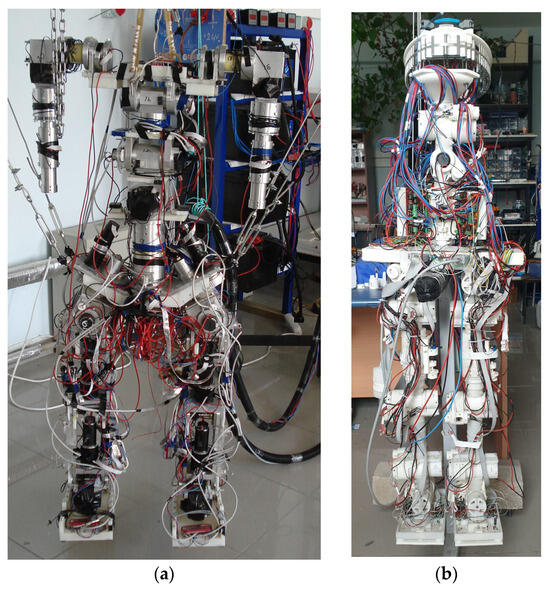
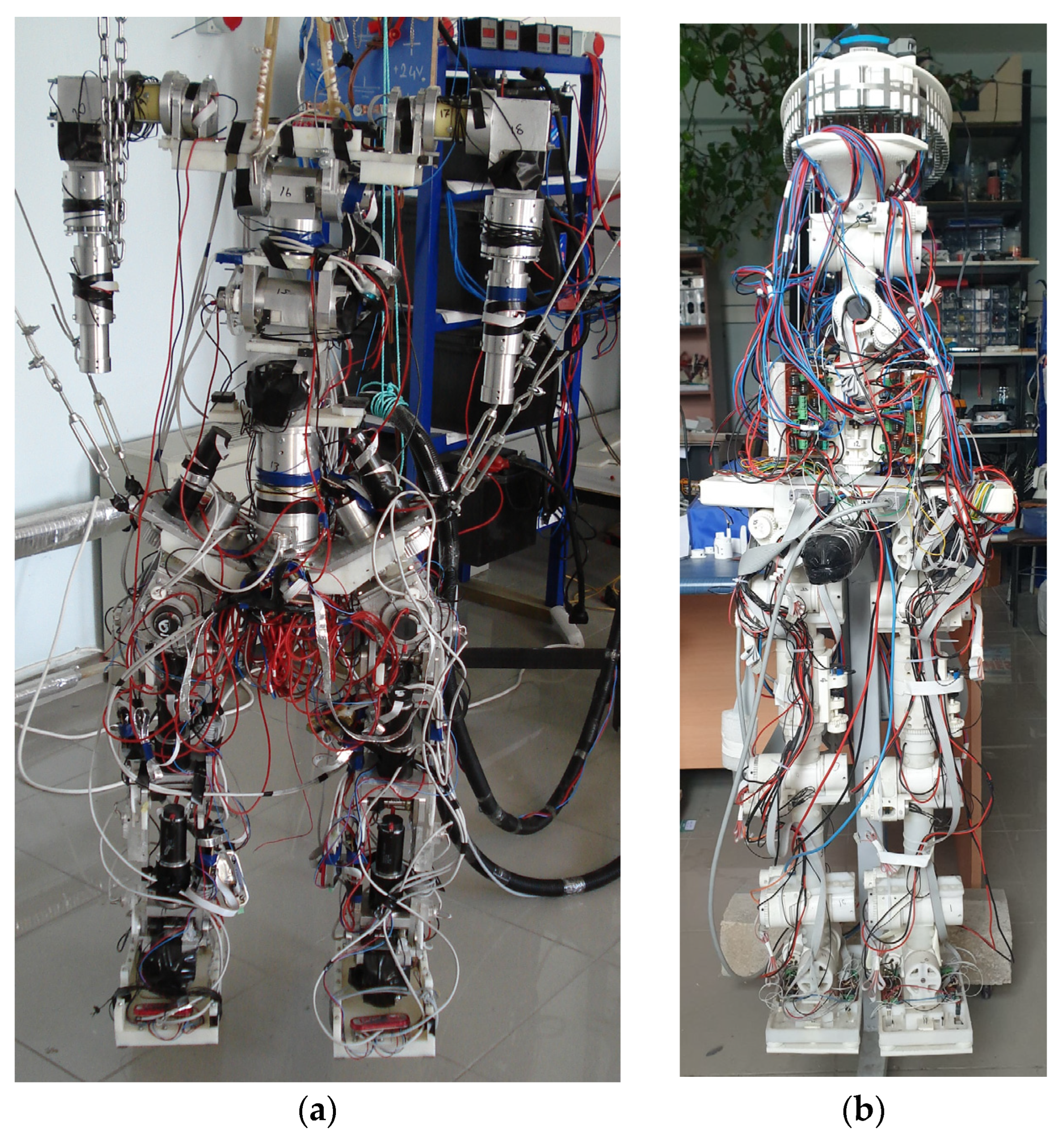
Secondly, the robot’s chosen structural material is Delrin, due to its wide availability, mechanical properties, and relative ease of machining. Therefore, the maximum torques and forces at the joints must be limited to remain within the motor sets’ and structural components’ limits. The structural components of RB2 were fabricated from Delrin (density: 1.42 g/cm³; tensile yield strength: 75.8 MPa). To achieve mass reduction while maintaining structural integrity, the load-bearing elements were designed with hollow cross-sections. This resulted in a humanoid robot weighing approximately 13 kg and standing 1.25 m tall, as compared to our previous humanoid robot named “BUrobot”, which was 55 kg and 155 cm. BUrobot’s structural parts were CNC-machined from aluminium (density 2.7 g/cc; tensile yield strength 276 MPa).

Aluminium has relatively lower stiffness and yield strength properties than a steel alloy. Therefore, some structural parts cannot be reduced in thickness, and to optimise the load-bearing capabilities of aluminium parts, they have to be designed with varying thicknesses and hollowed out to accommodate high gravitational and acceleration moments. Also, the unavailability of metal additive manufacturing capabilities and the fabrication of aluminium components with optimised internal lattice or cellular structures for enhanced stiffness-to-weight performance further complicate the design process. Therefore, RB2 was designed to explore lighter materials for its structural components. Figure 1 shows side-by-side pictures of BUrobot (a) and RB2 (b).

Figure 1. Past and present humanoid robots in our laboratory: (a) BUrobot; (b) RB2.

2.2. The Number of Degrees of Freedom and the Order of Joints

It is expected that the robot will be able to walk forward and backward and sideways, and change its direction of locomotion statically. Therefore, the robot’s legs have to have joints in all three planes of motion. For effective compensation of reaction forces and moments, the trunk mechanism has three degrees of freedom in all orthogonal planes. The design process subsequently requires specifying the degrees of freedom for the leg and trunk subsystems and systematically determining the link ordering within the overall kinematic chain. Table 1 provides a comparative overview of the degrees of freedom assigned to the leg and trunk mechanisms of selected humanoid robots, including their active development years and the corresponding joint motion orders within their kinematic structures. All the joints are ordered from the bottom to the top link, i.e., from the ankle joint to the hip joint. “A_RP” means the first ankle roll joint, then the ankle pitch joint. “K_P” means knee pitch joint, and “H_PRY” means at the lower side of the hip pitch, in the middle of the hip roll, and finally at the top of the hip yaw joint. Similarly, the trunk (R, P, Y) refers to the sequence of joints, where the roll joint is followed by the pitch joint, and at the top is the yaw joint. 2D_A_RP means that the robot has a 2D spherical ankle joint driven by linear screws. Similarly, the abbreviation 2D_T_RP denotes the analogous structural arrangement of the robot’s trunk mechanism. It is stated that the minimum number of degrees of freedom (DoF) required for locomotion is six [16], and almost all humanoid robots have six DoF in their legs, as shown in Table 1. The kinematic structures of the ankle and knee mechanisms in some actively developed humanoid robots share very similar design properties.

Table 1. Leg and trunk joint numbers and orders of some humanoid robots.

Robot	Leg DoF	Leg Joint Order	Trunk DoF	Trunk Joint Order
LRP 1999–2001 [17]	6	A_RP, K_P, H_PRY	0	0
H6 & H7 1999–2001 [18]	6	A_RP, K_P, H_PRY	0	0
ASIMO 2000–2018 [6]	6	A_RP, K_P, H_PRY	0	0
JAXON 2014–2015 [19]	6	A_RP, K_P, H_PRY	3	R, P, Y
TaeMu 2014–2016 [20]	6	A_RP, K_P, H_PRY	3	Y, R, P
HRP-4 2009–2010 [21] HRP-5P 2018 [22]	6	A_RP, K_P, H_PRY	3	P, R, Y
LOLA 2009 [23]	6 + 1 toe	2D_A_RP, K_P, H_PRY	2	Y, R
RH5 2020–2024 [24]	6	2D_A_RP, K_P, H_PRY	3	2D_T_RP, Y
ATLAS 2024 [10]	6	2D_A_RP, K_P, H_YRP	3	Y, 2D_T_RP
Agile ONE 2025 [11]	6	2D_A_RP, K_P, H_YRP	3	Y, 2D_T_RP
IRON 2025 [7]	6	2D_A_RP, K_P, H_RPY	3	Y, 2D_T_RP
Oli 2025 [5]	6	2D_A_RP, K_P, H_YRP	3	Y, 2D_T_RP
Figure 03 2025 [9]	6	2D_A_RP, K_P, H_YRP	3	Y, 2D_T_RP
Tesla Optimus 2025 [14]	6	2D_A_RP, K_P, H_PYR	2	R, Y
Adam 2025 [25]	6	2D_A_RP, K_P, H_YRP	3	R, P, Y

While the designs of the ankle and knee joints in current humanoid robots show a very similar ordering, the ordering of the hip joint motion planes varies. This is perhaps based on the designer’s experience and choice to use mathematical models. The trunk architecture of most humanoid platforms typically consists of a yaw joint followed by a two-degree-of-freedom spherical joint that provides pitch and roll from the bottom to the top of the trunk. The determination of the degrees of freedom and motion ranges for the trunk segment is ultimately governed by the designers’ choices.

We have chosen six degrees of freedom for the legs and three for the trunk in our humanoid robot RB2. A serial kinematic structure with joint-mounted actuators was selected to align with the use of non-metallic structural components and the limitations of the available fabrication infrastructure. The order of the joints from bottom to top is Roll-Ankle, Pitch-Ankle, Pitch-Knee, Yaw-Hip, Pitch-Hip, and Roll-Hip. This joint configuration has symmetry for ease of assembly, and placing the yaw joint between the knee and hip has kept the leg length to a minimum.

RB2’s trunk yaw joint is directly connected to the hip plate, which structurally integrates the upper and lower segments of the robot. This joint permits continuous rotation up to 360°, although the practical range of motion is constrained by cable routing from the lower limbs. The roll and pitch joints are positioned serially above the yaw joint within the trunk assembly. Notably, when the yaw joint undergoes a 90° rotation, the effective ordering of the subsequent trunk joints is reversed relative to the global reference frame.

2.3. Actuators of the Robot

The actuator selection and robots’ structural design require many iterations [6,26]. The robotic researchers utilise hydraulic, pneumatic, ultrasonic, and AC and DC motors. Early humanoid robots developed at Waseda University [27] and at Boston Dynamics have been powered by pneumatic actuators, such as ATLAS and WABOT, and by hydraulic actuators, such as PETMAN. Pneumatic actuators are also available in artificial pneumatic-muscle form and are used in robotic applications [28]. Both pneumatic and hydraulic actuators require relatively noisy pumps and have leak-prone hoses. However, recent advancements in hydraulic power units installed on the WLR-3P [29] enable remarkably high-speed motion and jumping capability. This is due to the wheel-and-leg fusion in their design, since it utilises the structure to carry hydraulic fluid without the need for hydraulic hoses. However, most contemporary humanoid robots use brushless direct current motors (BLDC). These types of motors produce high torque (when coupled with harmonic gearboxes) and are easy to control [1]. Leading research groups in humanoid robotics have been developing their own local controller boards for BLDC actuators [1,5,6,7,8,9,10,11,12,13,14,30]. Commercially available motor drivers usually do not meet the size, current, and communication requirements of humanoid robots. In some robotic applications, BLDC motors do not directly drive robot joints. A synchronous belt is used to transfer torque from the BLDC motor to the harmonic gear assembly [21,22,26,31]. If several links require actuation in a relatively small space, the most common way is to use guided steel tendons [1,30]. Additionally, series elastic elements are used after BLDC motor drives to enhance the actuation system’s dynamic range, enabling faster response to external impact forces [30].

In the present study, previously available motor–gearbox units were reutilised to reduce research costs and promote sustainable engineering practices. Consequently, the design iteration process was primarily focused on the robot’s structural components, influencing material selection, link dimensions, and the resulting mass and inertial properties.

2.4. Mathematical Modelling

Mathematical models are developed to understand the functions of biological systems and to simulate and control robots [32]. Ulbrich et al. stated that comprehensive dynamical models are essential for designing robot hardware components, stabilising controller systems, and generating locomotion trajectories [33].

Vukobratovic et al. [32] clearly explained the necessity of developing complex mathematical models not only to build functional robots but also to explore the biomechanical functions and behaviours of biological beings. The advanced humanoid robots that emerged in 2025, as noted in Table 1, use AI models and powerful processors to train on stabilising control systems and motion realisation [9]. In the RB2 humanoid robot, nonlinear kinematic models were employed to validate the iterative CAD-based structural designs and to ensure that the required static range of motion could be achieved by the DC geared actuators. Since we selected the motors and designed the structural parts for our robot RB2 to perform static locomotion, the resulting kinematic equations were sufficient, as in our previous two humanoid robots [34,35].

Different types of mathematical models are necessary for the locomotion of a bipedal robot. For high-speed walking, running, and jumping motions, full-body dynamical equations are necessary. For a 15-degree-of-freedom biped robot, the full-body nonlinear symbolic dynamical model is over a thousand pages long, and using this equation for online dynamic locomotion is impossible with today’s computing power (as given in Appendix A, the nonlinear kinematic model is only about four pages long). Therefore, some forms of simplification are applied to these equations to enable real-time solutions for online gait adjustment. Usually, full-body nonlinear dynamical equations are used in simulations to train the control system and to test the performance of the simplified dynamical equations, assessing whether they are sufficient to capture the required dynamics.

On the other hand, nonlinear kinematic equations, such as those presented in this article, are usually preferred when the robot performs delicate, precise movements and requires full-body coordination at low speeds. Since the full-body nonlinear kinematic equations are about many times shorter in length and significantly require less time than full-body nonlinear dynamical equations, powerful processors can solve them in near-real time. This allows for precise real-time trajectory generation at low speeds (static walking and object manipulations). Typical motions include robot hands performing delicate motions, or a humanoid robot crawling through previously unstructured, unmapped, and possibly very tight spaces like caves, or even through areas after an earthquake or disaster. Therefore, static and dynamical motions complement each other. This scenario is the same for human movement in constricted spaces, where slow yet precise whole-body movement is required to transit through them.

In this article, the static motion of the robot is expected for the following reasons. First, the robot’s structure cannot handle high dynamic loads. The second reason is that the motors cannot deliver more than 20 watts of power and 6 N m of torque. And thirdly, the robot’s static motion should be studied first, as it is the first step towards fully dynamic motion generation.

For dynamical motion, a set of full 3D nonlinear dynamical equations would be necessary. We left that work for our future generations of robots because RB2’s current motor sets cannot safely deliver high torques. The explicit development and formulation of the kinematic models for this robot will be discussed in a separate publication, as the complexity of the equations and their implementation warrants a detailed discussion. However, a brief discussion of the 3D nonlinear kinematic equation is given below. After mechanical integration and preliminary functional validation, a simulation-based control system will be implemented, with prospective incorporation of advanced artificial intelligence-based strategies.

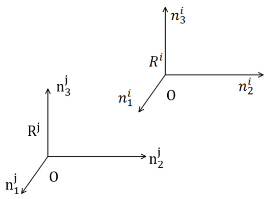
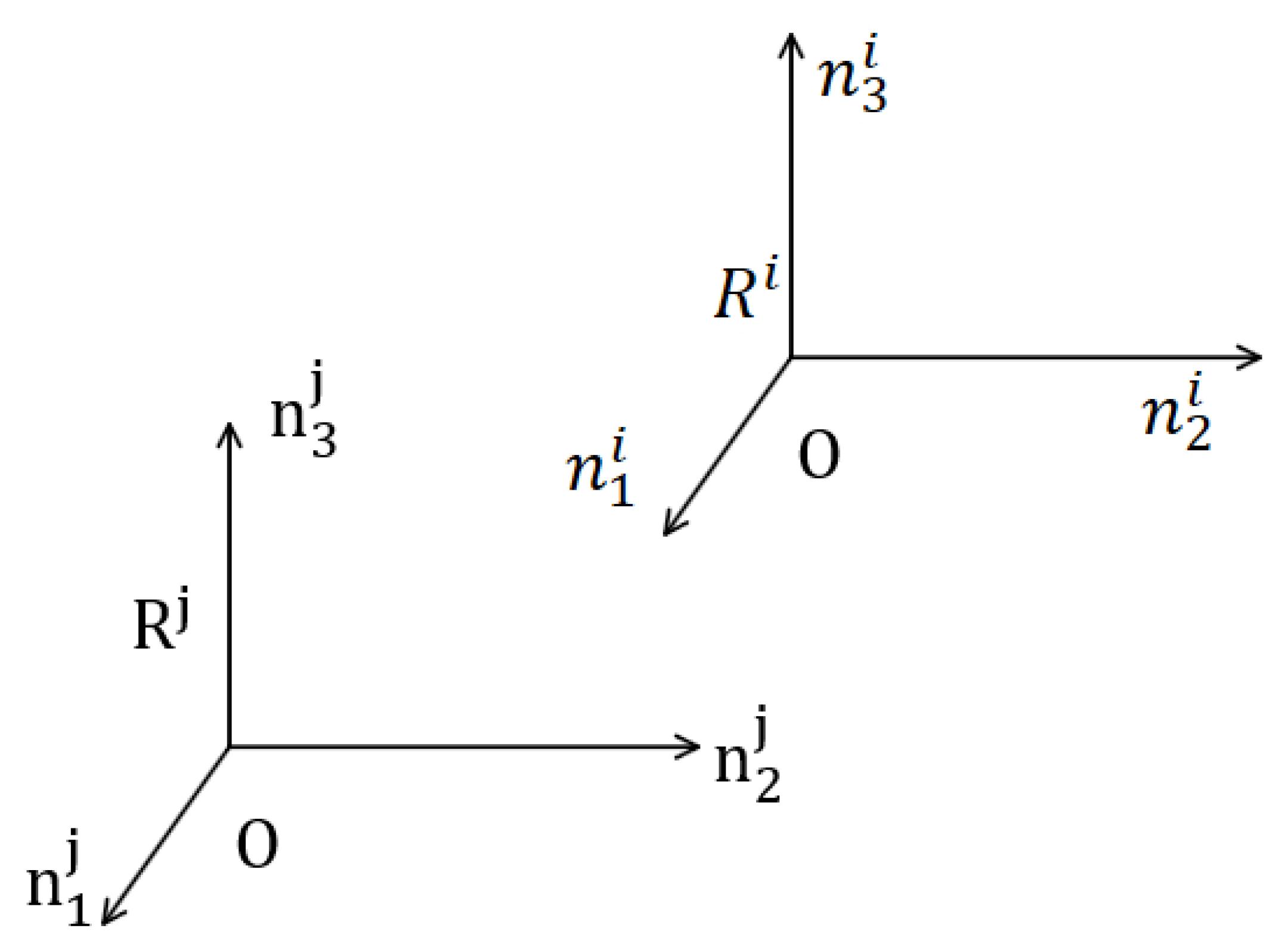
The mathematical model is based on an open tree configuration. The left foot is chosen to be firmly in contact with the ground. The tree branches after the hip’s roll joint into two. One branch goes up towards the trunk of RB2, and the other goes to the robot’s right leg. The stationary inertial reference frame is placed on the ground and named $R^0$ and then an inertial reference frame is placed at every joint’s base and named links, given a number as $R^i$ as shown in Figure 2.

Figure 2. Inertial reference frame. Here ${\overline{n}}_1^j$—the front, ${\overline{n}}_2^j$—the side, and ${\overline{n}}_3^j$—the vertical direction of the robot $j^{th}$ links.

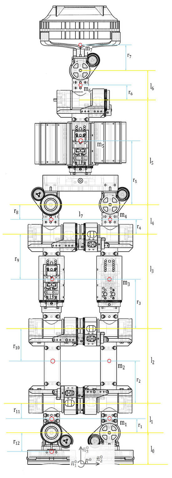
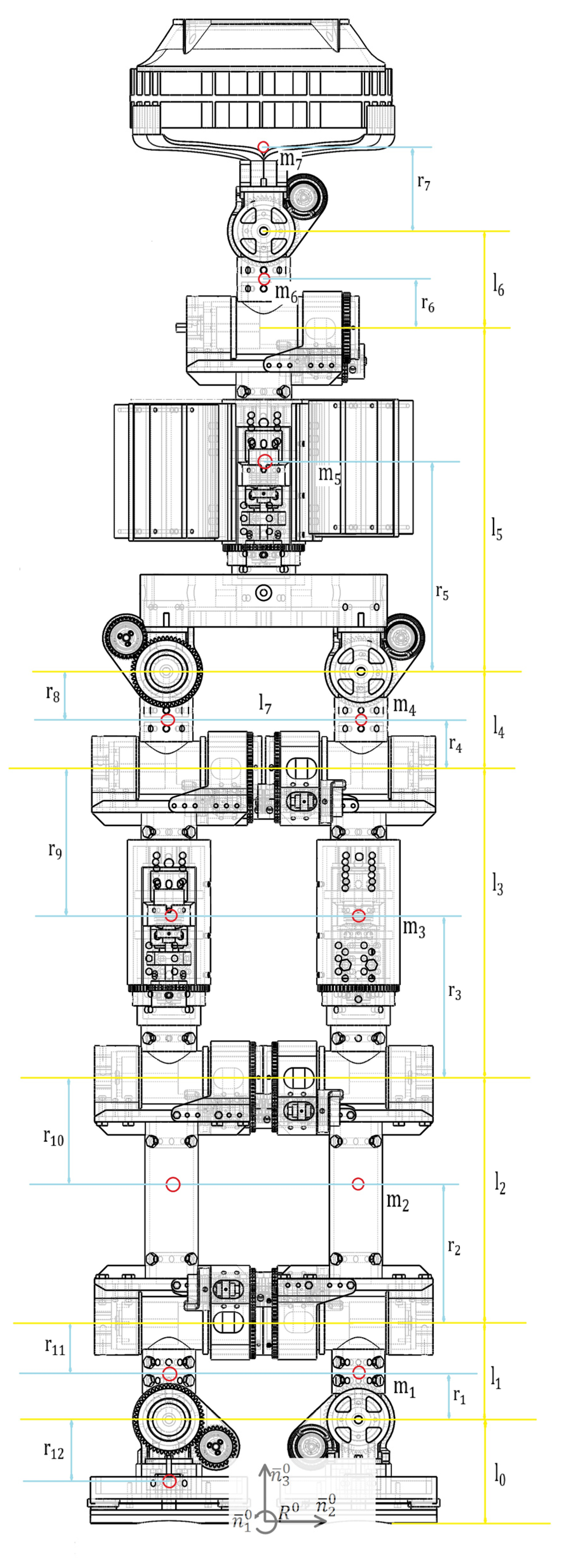
In Figure 3, the lumped masses of each link are indicated by $m_i$ $i=1,\cdots ,7$, the location of each link’s mass centre from its joint’s centre is $r_j$ $i=1,\cdots ,12$, and the distances between the robot joints are given by $l_j$ $i=1,\cdots ,7$. The inertial coordinate system is placed at the ground, and coordinate systems are placed at each joint axis. The yaw joints are neglected in this part of the kinematic equations, because the sagittal plane hip and knee joints require the highest torque ratings [21,33,36]. Due to the gravitational forces being absorbed by the yaw joint structure, with the whole robot’s moment of inertia about the vertical Iyy = 0.143 kgm² axis, and the robot taking a single step in about 10 s, the yaw motor only needs to generate a maximum of 0.5 Nm of torque to rotate its yaw joints in the legs. The rotation of the yaw joint does not change the vector sum of moment in the following joints in $n_1^i$ and $n_2^i$ directions. This is the result of our design objectives, as detailed in Section 3.2. The initial objective is to determine the moments induced in the pitch and roll joints of the RB2 by gravitational acceleration. The reference frames are named $R^0$ through $R^{12}$. Unit vectors along orthogonal axes in each reference frame are represented as $n_i^j$. Here, $i=\mathrm{1,2},3$ are the axis directions, and $j=1,\cdots ,12$ is the related reference frame.

Figure 3. The lumped masses, the mass centre locations, and distances between the joints are given as, $m_i$ $i=1,\cdots ,7$, $r_j$ $i=1,\cdots ,12$ and $l_j$ $i=1,\cdots ,12$.

The orthonormal transformation matrices between the $R^i$ reference frames $R^j$ (Figure 2) are given as $S^{1j}$. The transformation matrices are well known in the robotic community, and brief details are given in [37]. The transformation matrices are multiplied by succeeding ones to obtain the absolute transformation between any joint and the ground $S^{i0}$. Starting from the support foot’s roll joint axis, the kinematic chain can be written as below.

$${\mathrm{T}}_1={\displaystyle \sum _{\mathrm{i}=1}^{12}}\left({\overline{\mathrm{p}}}_{\mathrm{i}}+{\overline{\mathrm{l}}}_{\mathrm{i}}\right)\times {\mathrm{m}}_{\mathrm{i}}.\overline{\mathrm{g}}$$

(1)

In Equation (1), $T_1$ represents the moment induced by the gravitational acceleration in joint 1. ${\overline{p}}_i$ represents the mass location from its origin of reference frame attached to the $i^{th}$ joint. $\overline{g}$ is gravitational acceleration, which in vector form is $\overline{g}=\left[\begin{array}{cc}0& \begin{array}{cc}0& -g\end{array}\end{array}\right]$. Below, the upper index $T$ represents the transpose of the vector.

$$\begin{array}{c}{\overline{p}}_1={\left[0 0 r_1\right]}^T,{\overline{p}}_2={\left[0 0 r_2\right]}^T,{\overline{p}}_3={\left[0 0 r_3\right]}^T,{\overline{p}}_4={\left[0 0 r_4\right]}^T,{\overline{p}}_5={\left[0 0 r_5\right]}^T,{\overline{p}}_6={\left[0 0 r_6\right]}^T,\hfill \\ {\overline{p}}_7={\left[0 0 r_7\right]}^T,{\overline{p}}_8={\left[0 0 {-r}_8\right]}^T,{\overline{p}}_9={\left[0 0 {-r}_9\right]}^T,{\overline{p}}_{10}={\left[0 0 {-r}_{10}\right]}^T,{\overline{p}}_{11}={\left[0 0 {-r}_{11}\right]}^T,{\overline{p}}_{12}={\left[0 0 r_{12}\right]}^T\hfill \end{array}$$

Equation (1) is rewritten as Equation (2), which is evaluated symbolically. The result is $3\times 3$ a moment matrix calculated for joint one in the open tree structure, which is the left ankle’s roll joint. Since the modular robot joint structures are designed to allow only moment along the motor shaft’s axis, we can safely ignore the remaining moment components. In this analysis, we are only interested in the moment at which the motor must counteract and rotate the joint.

Appendix A gives the result of the symbolic calculation of Equation (2). $T_1\left(1\right)$ is the moment induced by gravity in the support ankle’s roll joint about its axis of rotation (it is $n_1^1$) and $T_1\left(2\right)$ is the moment induced by gravity in the support ankle’s roll joint ($n_2^1$). $T_1\left(2\right)$ is counteracted by the support structure of the roll joints. Since the yaw joints are not included in the nonlinear kinematic equation calculations, the $T_1\left(3\right)$ component is equal to zero. The equation given in Appendix A is the moment at the first joint in the open tree structure. Therefore, using this equation, the moments in other joints can be easily obtained. These equations enable the simulation of different robot configurations. For instance, if all joint angles and masses of the links are set to zero except the swing leg ones, the moments induced by gravitational acceleration can be calculated at the swing hip joints.

Although the equations in Appendix A are relatively lengthy, the linearization and simulation are performed via custom-written MATLAB functions. As mentioned before, a detailed explanation of the neglected aspects in this paper will be provided in subsequent studies.

$$\begin{array}{c}{T}_1=m_1.\overline{g}\times (r_1.{\overline{n}}_3^1.S^{10})\hfill \\ {+m}_2.\overline{g}\times (l_1.{\overline{n}}_3^1.S^{10}+r_2.{\overline{n}}_3^2.S^{20}) \hfill \\ +m_3.\overline{g}\times (l_1.n_3^1.S^{10}+l_2.n_3^2.S^{20}+r_3.n_3^3.S^{30})\hfill \\ +m_4.\overline{g}\times (l_1.{\overline{n}}_3^1.S^{10}+l_2.{\overline{n}}_3^2.S^{20}+l_3.{\overline{n}}_3^3.S^{30}+r_4.{\overline{n}}_3^4.S^{40})\hfill \\ +m_5.\overline{g}\times (l_1.{\overline{n}}_3^1.S^{10}+l_2.{\overline{n}}_3^2.S^{20}+l_3.{\overline{n}}_3^3.S^{30}+l_4.{\overline{n}}_3^4.S^{40}+r_5.{\overline{n}}_3^5.S^{50})\hfill \\ +m_6.\overline{g}\times (l_1.{\overline{n}}_3^1.S^{10}+l_2.{\overline{n}}_3^2.S^{20}+l_3.{\overline{n}}_3^3.S^{30}+l_4.{\overline{n}}_3^4.S^{40}+l_5.{\overline{n}}_3^5.S^{50}+r_6.{\overline{n}}_3^6.S^{60})\hfill \\ +m_7.\overline{g}\times (l_1.{\overline{n}}_3^1.S^{10}+l_2.{\overline{n}}_3^2.S^{20}+l_3.{\overline{n}}_3^3.S^{30}+l_4.{\overline{n}}_3^4.S^{40}+l_5.{\overline{n}}_3^5.S^{50}+l_6.{\overline{n}}_3^6.S^{60}\hfill \\ \hspace{1em}\hspace{1em}\hspace{1em}\hspace{1em}\hspace{1em}\hspace{1em}+r_7.{\overline{n}}_3^7.S^{70})\hfill \\ +m_8.\overline{g}\times (l_1.{\overline{n}}_3^1.S^{10}+l_2.{\overline{n}}_3^2.S^{20}+l_3.{\overline{n}}_3^3.S^{30}+l_4.{\overline{n}}_3^4.S^{40}+l_5.{\overline{n}}_3^5.S^{50}+l_6.{\overline{n}}_3^6.S^{60}\hfill \\ \hspace{1em}\hspace{1em}\hspace{1em}\hspace{1em}\hspace{1em}\hspace{1em}+{(-l}_7).{\overline{n}}_2^7.S^{70}+(-r_8).{\overline{n}}_3^8.S^{80})\hfill \\ +m_9.\overline{g}\times (l_1.{\overline{n}}_3^1.S^{10}+l_2.{\overline{n}}_3^2.S^{20}+l_3.{\overline{n}}_3^3.S^{30}+l_4.{\overline{n}}_3^4.S^{40}+l_5.{\overline{n}}_3^5.S^{50}+l_6.{\overline{n}}_3^6.S^{60}\hfill \\ \hspace{1em}\hspace{1em}\hspace{1em}\hspace{1em}\hspace{1em}\hspace{1em}+{(-l}_7).{\overline{n}}_2^7.S^{70}+{(-l}_4).{\overline{n}}_3^8.S^{80}+{(-r}_9).{\overline{n}}_3^9.S^{90})\hfill \\ +m_{10}.\overline{g}\times (l_1.{\overline{n}}_3^1.S^{10}+l_2.{\overline{n}}_3^2.S^{20}+l_3.{\overline{n}}_3^3.S^{30}+l_4.{\overline{n}}_3^4.S^{40}+l_5.{\overline{n}}_3^5.S^{50}+l_6.{\overline{n}}_3^6.S^{60}\hfill \\ \hspace{1em}\hspace{1em}\hspace{1em}\hspace{1em}\hspace{1em}\hspace{1em}+{(-l}_7).{\overline{n}}_2^7.S^{70}+{(-l}_4).{\overline{n}}_3^8.S^{80}+{(-l}_3).{\overline{n}}_3^9.S^{90}+{(-r}_{10}).{\overline{n}}_3^{10}.S^{100})\hfill \\ +m_{11}.\overline{g}\times (l_1.{\overline{n}}_3^1.S^{10}+l_2.{\overline{n}}_3^2.S^{20}+l_3.{\overline{n}}_3^3.S^{30}+l_4.{\overline{n}}_3^4.S^{40}+l_5.{\overline{n}}_3^5.S^{50}+l_6.{\overline{n}}_3^6.S^{60}\hfill \\ \hspace{1em}\hspace{1em}\hspace{1em}\hspace{1em}\hspace{1em}\hspace{1em}+{(-l}_7).{\overline{n}}_2^7.S^{70}+{(-l}_4).{\overline{n}}_3^8.S^{80}+{(-l}_3).{\overline{n}}_3^9.S^{90}+{(-l}_2).{\overline{n}}_3^{10}.S^{100}\hfill \\ \hspace{1em}\hspace{1em}\hspace{1em}\hspace{1em}\hspace{1em}\hspace{1em}+{(-r}_{11}).{\overline{n}}_3^{11}.S^{110})\hfill \\ +m_{12}.\overline{g}\times (l_1.{\overline{n}}_3^1.S^{10}+l_2.{\overline{n}}_3^2.S^{20}+l_3.{\overline{n}}_3^3.S^{30}+l_4.{\overline{n}}_3^4.S^{40}+l_5.{\overline{n}}_3^5.S^{50}+l_6.{\overline{n}}_3^6.S^{60}\hfill \\ \hspace{1em}\hspace{1em}\hspace{1em}\hspace{1em}\hspace{1em}\hspace{1em} +{(-l}_7).{\overline{n}}_2^7.S^{70}+{(-l}_4).{\overline{n}}_3^8.S^{80}+{(-l}_3).{\overline{n}}_3^9.S^{90}+{(-l}_2).{\overline{n}}_3^{10}.S^{100}\hfill \\ \hspace{1em}\hspace{1em}\hspace{1em}\hspace{1em}\hspace{1em}\hspace{1em} +{(-l}_1).{\overline{n}}_3^{11}.S^{110}+{(-r}_{12}).{\overline{n}}_3^{12}.S^{120})\hfill \end{array}$$

(2)

3. Details of Robot Joints

3.1. The Foot

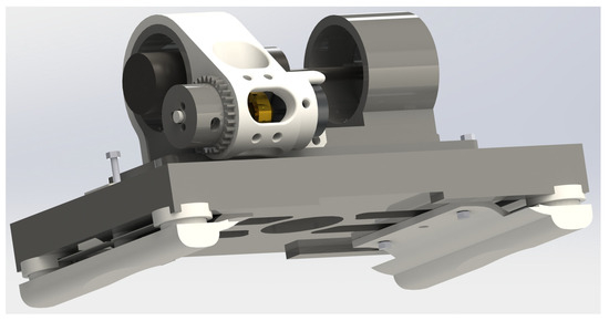
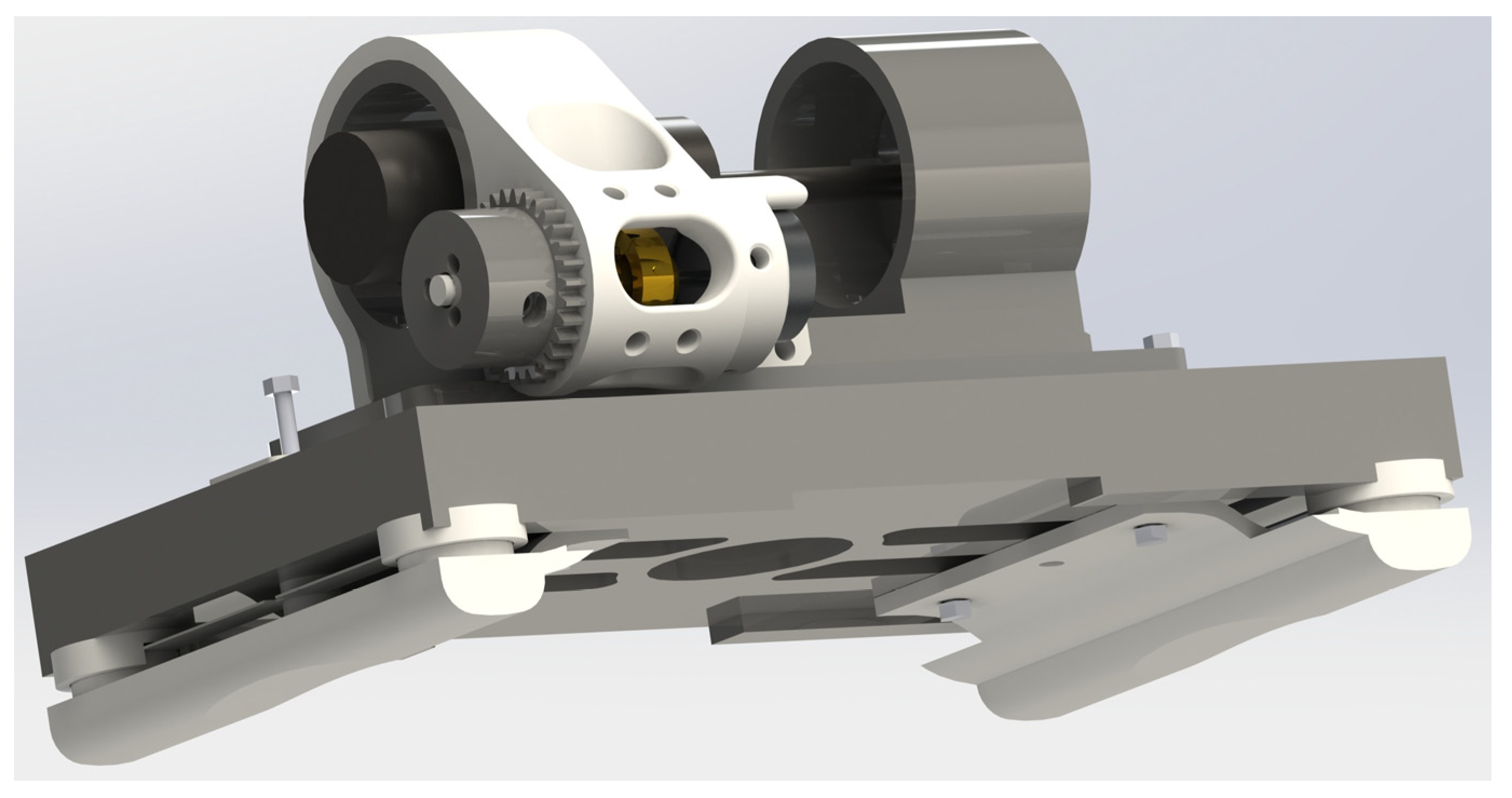
Yamamoto [38] have neatly reviewed various toe mechanisms and given a detailed explanation of their mechanical designs for humanoid robots. Ref. [33] claimed that, in their humanoid robot LOLA, the active toe joint enables more natural locomotion. However, humanoid robots such as Figure 03 and Atlas performed natural walking cycles without an active toe joint. We share the same view on the advantages of utilising a passive or active toe joint, but the Figure 03 humanoid robot and the advanced robots in 2025 have shown the importance of adaptive locomotion using AI models running on 275 TOPS processors. Therefore, greater emphasis should be placed on collecting and analysing data from the robot’s sensors to facilitate the efficient generation of an adaptive control and locomotion strategy. In this regard, no toe joint was incorporated into the RB2 humanoid robot, as shown in Figure 4. RB2 has a round semi-cylindrical part in both the heel and toe sections of the foot. The foot components fulfil two primary functions: (1) acquisition of ground reaction pressure data under the foot using force-sensitive resistor (FSR) sensors, and (2) facilitation of a rolling contact mechanism throughout the landing (heel-strike to mid-stance) and take-off (push-off) phases of bipedal locomotion.

Figure 4. The foot of RB2.

Force-sensitive resistor (FSR) sensors are commonly employed in lightweight robotic platforms [39]. Due to their relative fragility and sensitivity to off-axis loading, the sensors were housed within cylindrical enclosures designed to permit only vertically oriented ground reaction forces.

3.2. The Leg and the Trunk Design

The robot’s dimensions are primarily determined by the available electric motors and the robot’s overall symmetry. The primary tool for designing humanoid robots is SolidWorks [40]. Our design objectives for the robot joints as follows:

Modular design: We want to use the same joint structure, motor sets, and electronic drive system to reduce production costs and the robot’s complexity, increase interchangeability, and ease maintenance and repairs.

The design cocoons the motor sets against external impacts and allows only axial loads on the motor gearbox shaft.

Non-metallic structural parts protect the motor and circuitry from electrostatic discharge risks. Although the circuitry has a ground connection, this non-metallic structure provides additional safety, which we experienced issues with in our previous humanoid robot [35].

The robot’s weight is kept to a minimum without compromising structural stiffness [41].

The robot is designed with a left–right and anterior–posterior symmetric joint architecture, which is expected to expand the feasible space for joint trajectory generation. In particular, due to the absence of a kneecap mechanism, the robot is anticipated to achieve locomotion with the knee joint operating at unconventionally negative angular configurations.

The sagittal plane hip and knee joints require the highest torque ratings [21,33,36]. The yaw joint of the leg is placed between the knee and the pitch joint of the hip. This allowed for minimising the leg size and simplifying the hip assembly. Since the highest torques are observed especially in the knee and hip pitch joints, the hip pitch joint is placed lower in the assembly. The hip roll joints require relatively smaller torque values [21,33,36]; therefore, this joint sits on top of the hip assembly. Therefore, if the motor sets’ ratings are calculated for these two joints, it is safe to state that the other joints’ power/torque requirements are sufficiently met. The required torque to counteract the moment due to gravitational acceleration can be obtained from a simple lumped-mass inverted-pendulum-mode calculation, as given in [21]. However, in the appendix, we provide equations for the frontal and side axes to calculate the exact torque requirement for each joint of the robot. By setting the relevant masses and relative angles to zero in the two equations for the roll joint of the support leg, the torque requirement for the other joints can be obtained.

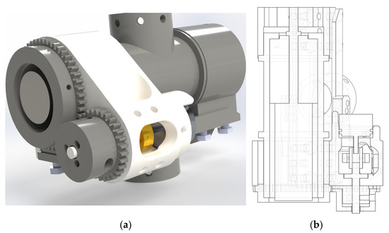
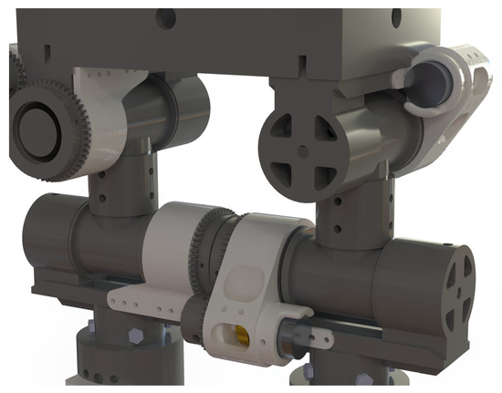
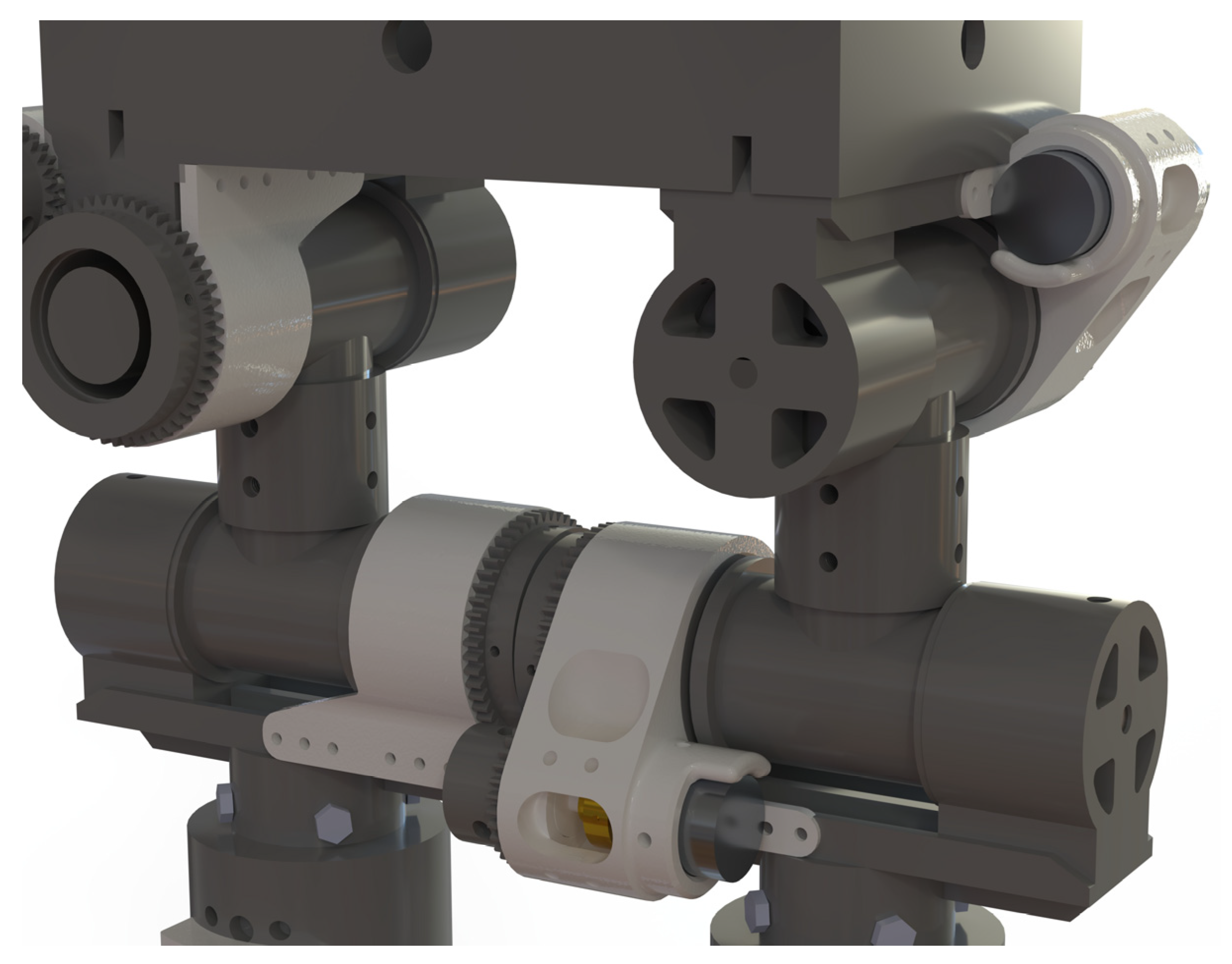
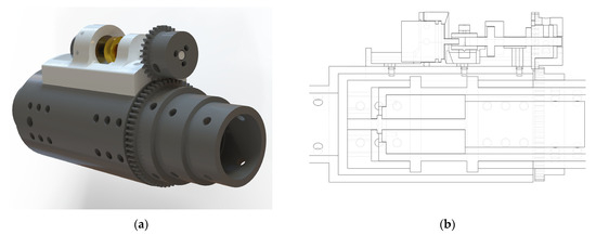
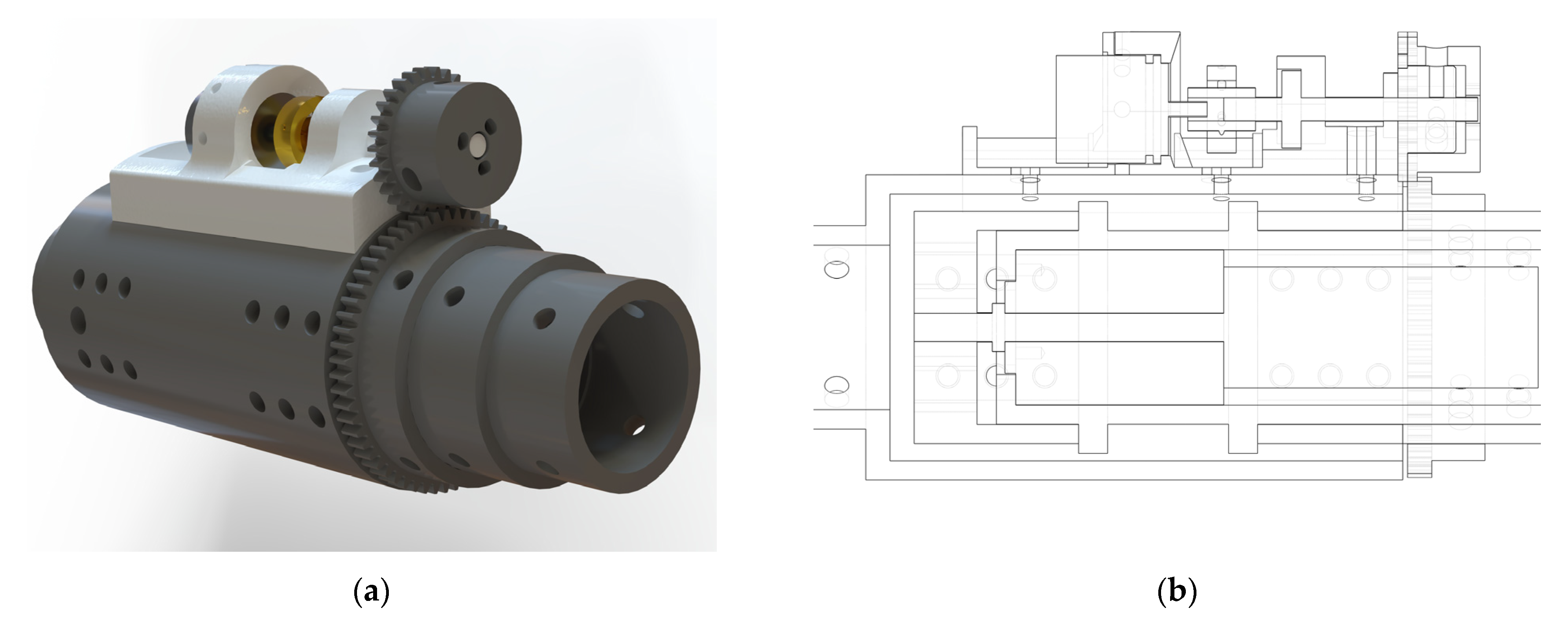
RB2 is expected to walk statically and with relatively small step lengths. For a step length of approximately 20 cm, the knee joint requires about 2.5 Nm of torque, which is within the gearboxes’ 5 Nm nominal torque rating. Figure 5 shows rendered (Figure 5a) and wireframe section (Figure 5b) views of the modular robot link that is used in a total of 12 sagittal and lateral plane joints of the robot’s legs and trunk. A close-up of the hip section is shown in Figure 6. As seen here, by assembling the identical joint structures at right angles to each other, the hip roll and hip pitch joint structure is obtained.

Figure 5. The modular joint structure is used in all the robot’s sagittal and lateral joints. (a) The rendered view of the joint structure; (b) sectioned view of the joint in wireframe.

Figure 6. A close-up view of the robots’ modular hip joint assembly in the lateral and sagittal planes.

Usually, hip and shoulder joints have three degrees of freedom, and the rotational axes intersect at a point [22,23,31]. RB2 has intersecting ankle, hip, and trunk joints, as do almost all humanoid robots. It is stated that this geometric arrangement simplifies kinematic equations and their associated calculations and allows humanoid robots to achieve human-like motion [21,23,31]. However, the symbolic computation capabilities of software packages such as MATLAB 2022a and Mathematica have substantially reduced the mathematical burden of complex kinematic equations on researchers compared to two decades ago.

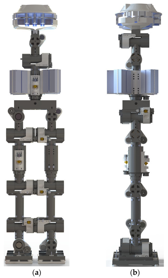
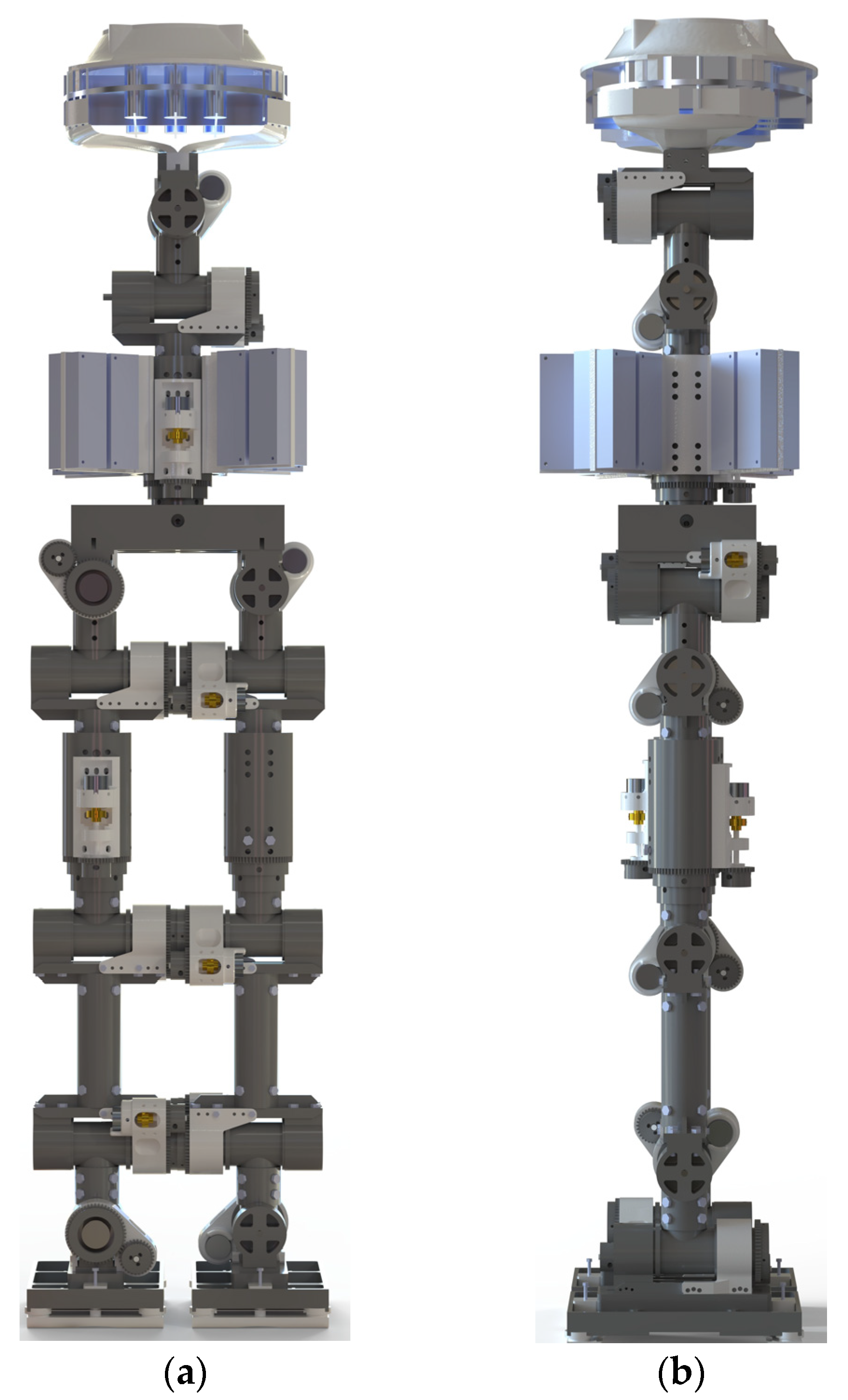
Figure 7 shows the front (a) and side-view (b) rendered images of the robot. As shown in this figure, the robot’s joints consist of only two modular structures. In this way, we have achieved all our design objectives. The close-up view provides a detailed illustration of the arrangement of the identical modular units in the pitch and roll joints of RB2.

Figure 7. Rendered images of RB2 in front and side planes. (a) The front view of RB2; (b) the side view of RB2.

Figure 8 shows the modular joint structure used in all three yaw axes of the robot’s legs and trunk. Figure 8a is a rendered view, and (b) is a sectioned view. The robot has a total of 15 joints, which was achieved using only two types of modular drive units. This modular architecture simplifies manufacturing, assembly, and maintenance while reducing overall system costs, a critical consideration given the limited project budget. Consistent with the design objectives, the trunk of RB2 employs a serial-joint configuration. Except for Tesla Optimus, most contemporary humanoid robots employ trunk mechanisms based on linear actuator-driven two-degree-of-freedom configurations, as summarised in Table 1 (2D_T_RP). In this way, an independent yaw joint is usually placed below the 2D spherical structure, combining structural rigidity about the pitch and roll axes while maintaining a relatively larger yaw rotation range. Humanoid robot trunks with Stewart mechanisms are also designed, and it is stated that they have higher stiffness but a lower rotation-angle range [40]. Similar 2D linear motor-driven mechanisms (2D_A_RP) are employed in the trunks of most current robots, except in a number of humanoid robots [16,39,41].

Figure 8. The modular joint structure is used in all the robot’s yaw joints. (a) Rendered view; (b) sectioned view.

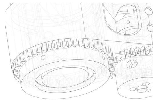
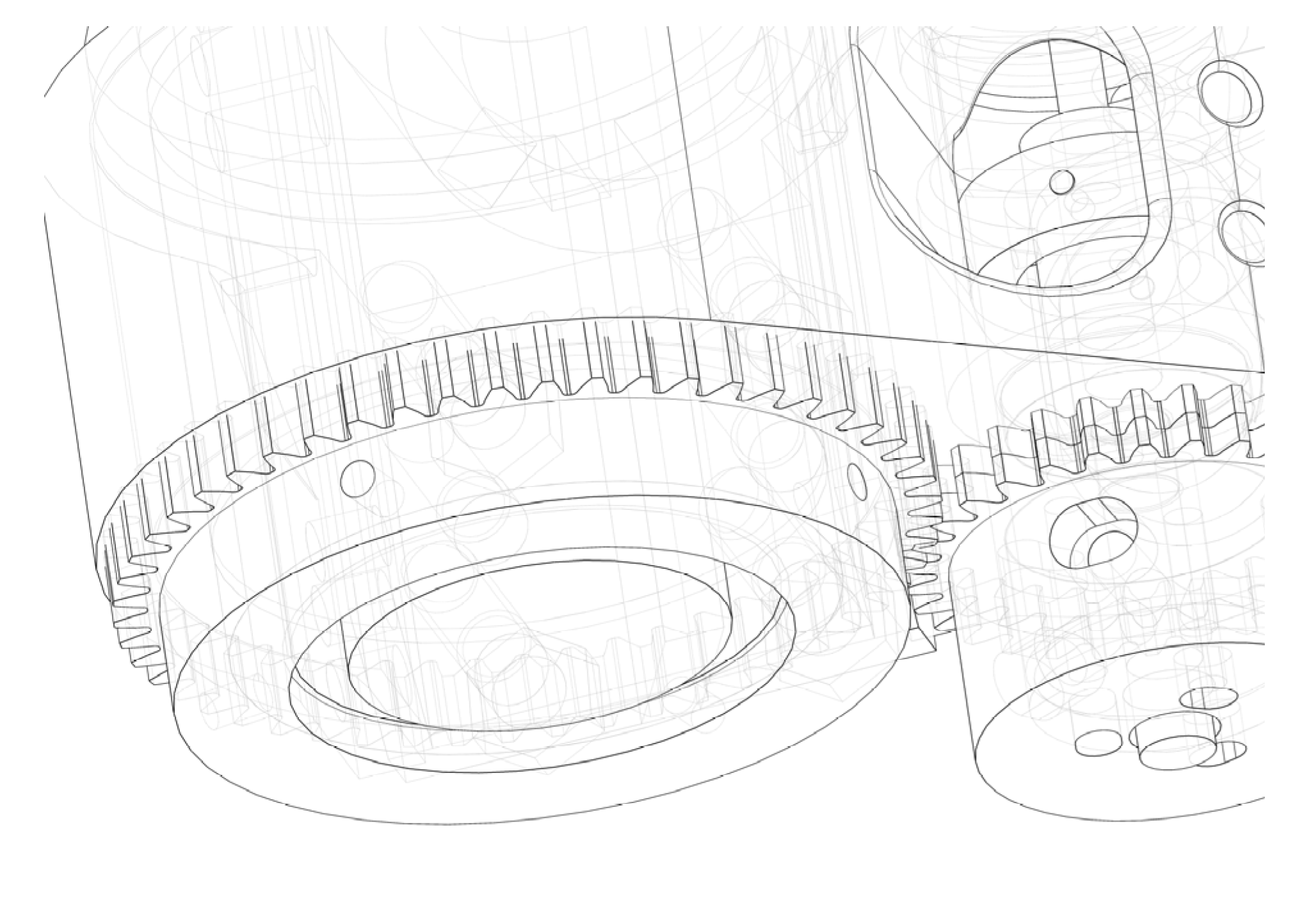
The potentiometers are mounted on the joint shafts via a spur gear pair, with the potentiometer shaft coupled to offset-adjustable coaxial spur gears, as illustrated in Figure 9. The backlash is eliminated by adjusting the relative offset amount of the double spur gears. This design principle is employed in a wide range of engineering applications to nullify backlash.

Figure 9. Offset dual spur gears are used to minimise backlash between the pairing gear teeth.

3.3. Electronics and Sensors

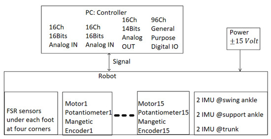
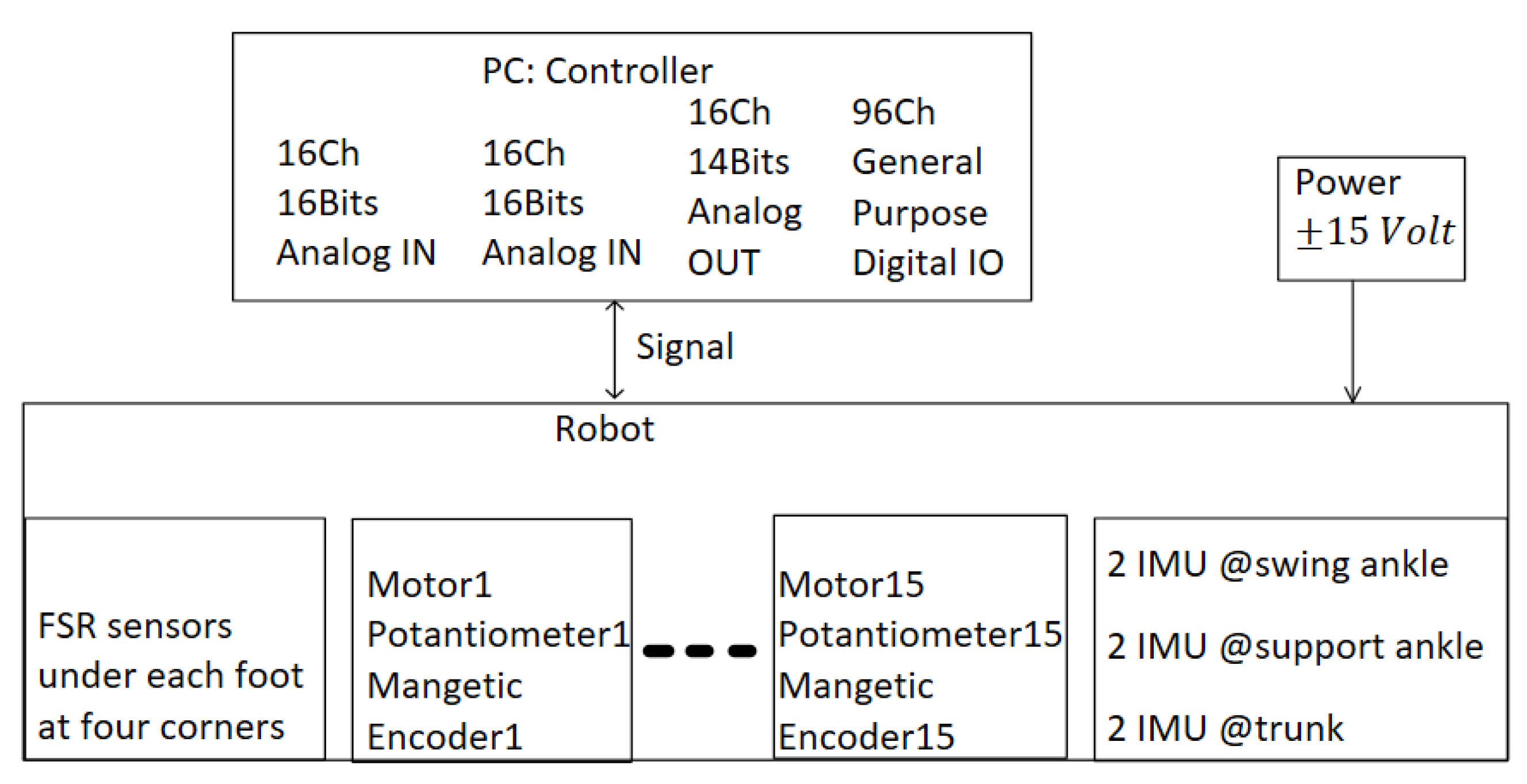
As depicted in Figure 10 below, the robot’s control system will run on an off-board PC. Four data acquisition cards read and send data. Two 16-channel differential-input acquisition cards with 16-bit resolution will be used to sample data from the potentiometer and FSR sensors at 10 ms intervals. A 14-bit, 16-channel analogue output card will be utilised to transmit control signals to power amplifier boards that drive the geared Maxon motors, while a 96-channel general-purpose digital I/O card will be employed to acquire digital states. The FSR sensors provide an approximate pressure distribution map at the foot–ground interface, with sensors positioned at the four corners of each foot. Additionally, six BNO055 absolute orientation inertial measurement units (IMUs) will be used to measure linear acceleration, absolute orientation, and the direction of Earth’s magnetic field. These sensors will be mounted in pairs, with each pair oriented orthogonally (90 degrees relative to one another) at the same locations on each leg and the trunk, to enhance overall measurement accuracy through redundancy and complementary data fusion.

Figure 10. Electronic and control units of the RB2 robot.

3.4. Dimensions and Weight

The masses, mass locations, and inertia properties of robot links are all obtained using SolidWorks 2017 SP 5.0 software [41,42]. The modular joint shown in Figure 5, which is used in all the lateral and sagittal plane joints, weighs about 579 g (all twelve of them weigh 6948 g), while the modular joint used in all yaw joints weighs about 686 g (three of them weigh 2058 g). A 190:1 three-stage gearbox with a 20-watt motor and an encoder weighs about 311 g. This motor set is used for all the robot’s joints (15 of them weigh 4665 g). The total weight of our humanoid robot in its current state (excluding cables) is approximately 12,975 g. The total of 15 motor assemblies weighs about 36% of the RB2’s total weight. Our humanoid robot RB2’s single foot plate, machined from Delrin, weighs approximately 388 g. The electronic hardware, including the power amplifier and filter circuits, their housing, and the cooling plate, contributes approximately 2768 g. The motor housings and load-bearing structural components account for approximately 4766 g, which is 36.7% of the total system mass of RB2. Structural components and actuation units (motors and gearboxes) account for 42% and approximately 31% of the LOLA humanoid robot’s total mass, respectively [23]. RB2 has slightly less structural weight, while the motor sets weigh a bit more than those of the humanoid robot LOLA [23]. The robot’s structural components account for a significant portion of its total weight, especially in early humanoid robots [4,26]. Since the structural parts are passive components that do not contribute to power generation or similar functions, their mass and moments of inertia must be minimised. What makes the structural parts of earlier robots relatively old is the manufacturing technology used to produce them. Mechanical component production has transitioned from traditional casting and three-degree-of-freedom (3-DOF) CNC machining to advanced manufacturing techniques, including 3D additive printing of metals and polymers and five-degree-of-freedom (5-DOF) CNC machining [7,9,10,14,43]. Although detailed mass-distribution data for contemporary leading humanoid robots are not publicly available, it is reasonable to assume that their weight distribution follows similar trends, with structural components becoming lighter and actuator assemblies heavier than in earlier generations.

Table 2 gives the range of angles that RB2’s joint can realise. Motion of the yaw joints is restricted solely by cable length. Mechanical interference imposes further constraints on the trunk: the roll joint is limited by the onboard circuit boards, and the pitch joint is constrained by contact with the power electronics cooling plate.

Table 2. Working angles of robot joints.

Trunk	Pitch	−55 to 55 degrees
	Roll	−60 to 60 degrees
	Yaw	−360 to 360 degrees
Hip	Roll	−3 to 113 degrees
	Pitch	−69 to 72 degrees
	Yaw	−360 to 360 degrees
Knee	Pitch	−140 to 132 degrees
Ankle	Pitch	−69 to 72 degrees
	Roll	−52 to 61 degrees

Table 3 provides the distances from the ground to the joints and the centre of mass location in the vertical direction relative to ground level. The distance between the vertical axes of the two legs is only 149 mm. The smaller the distance, the less trunk and lateral motion is required to shift the centre of mass sideways (z direction) [31]. The vertical location of the centre of mass should be near the hip joints. In this way, the robot’s locomotion becomes more stable [23,33]. RB2’s centre of mass is only off by 15 mm from its hip pitch joint’s axis. The humanoid robot RB2 has a total height of 1151.07 mm and a mass of 12,975 g, with its centre of mass positioned to approximate that of a human as reported in the literature [44].

Table 3. Distances between the joint axes.

Ground to ankle roll joint, $l_0$	78.65 mm
Ankle roll joint to ankle pitch joint, $l_1$	74 mm
Ankle pitch joint to knee pitch joint, $l_2$	188 mm
Knee pitch joint to hip pitch joint, $l_3$	237 mm
Hip pitch joint to hip roll joint, $l_4$	74 mm
Distances between the vertical axes of two legs, $l_5$	149 mm
Hip roll joint to trunk roll joint, $l_6=l_1$	263 mm
Trunk roll joint to trunk pitch joint, $l_7$	74 mm
Hip pitch joint to ground, $l_0+l_1+l_2+l_3$	577.65 mm
Centre of mass in vertical	563.17 mm

4. Analysis and Simulation

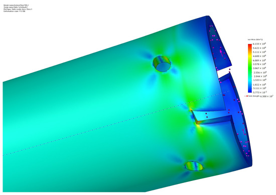
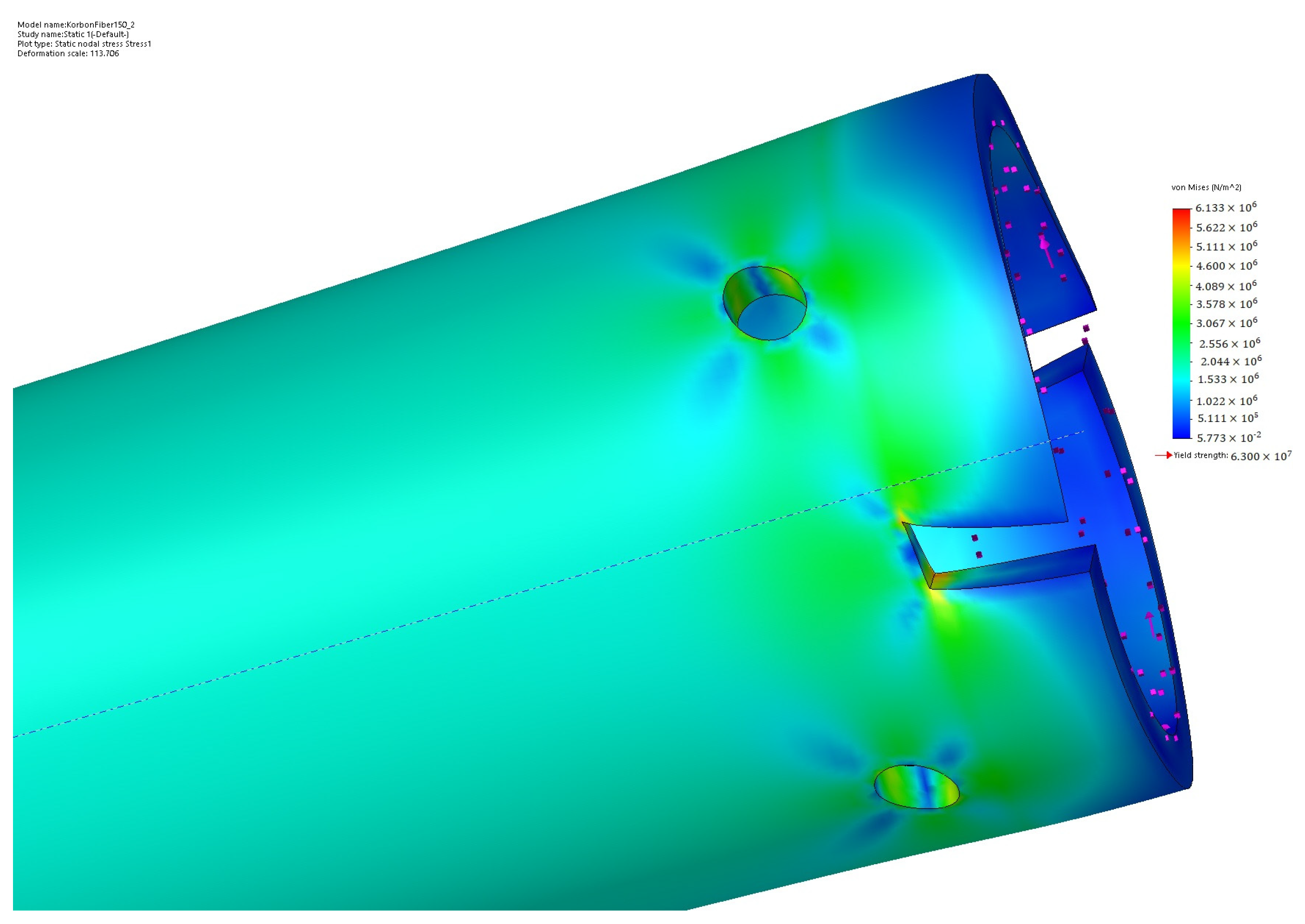
Figure 11 shows the stress distribution when a 6 Nm torque difference is applied between the robot joints. In this figure, the highest stress is 6.133 MPa. At this nominal torque level, the stress is about 10% of Delrin’s yield strength. This Delrin part is located between the pitch ankle and knee joints, and between the knee and pitch hip joints. The motors used in the robots can continuously deliver a nominal torque of 6 Nm, which is one reason for the robot’s expected static motion. In this torque range, a 3 mm thickness for the hollowed-out parts is sufficient. This design choice results in a weight reduction of about 75% and a reduction in motor power requirements from 90 watts to 20 watts.

Figure 11. Stress distribution when 6 Nm torque is applied. The red dots and arrow are the applied torques and their direction.

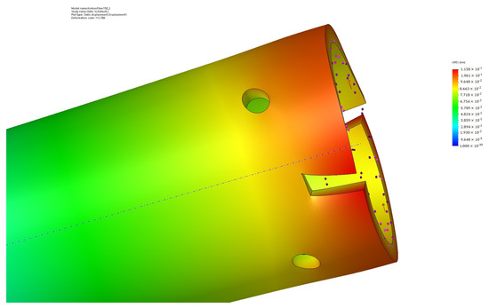
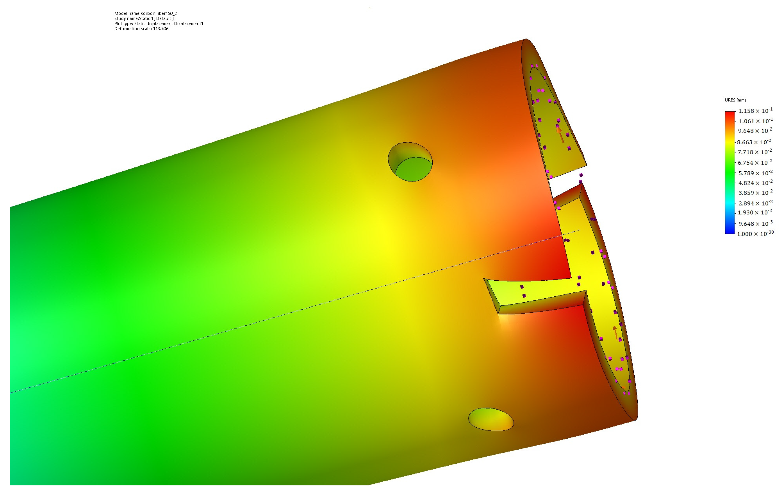
Figure 12 shows the displacement distribution when a 6 Nm torque difference is applied between the robot joints. In this figure, the maximum displacement is 0.1158 mm. Concerning the joint length between the ankle and the knee, this displacement results in 0.028 degrees of angular deviation at this torque level. The angle is negligible [45] during static locomotion; however, it is not negligible during dynamic motions. This is one of the reasons RB2 will be performing only static locomotions. Robot joints and, as a whole, the robot’s structure require rigidity for the joints to follow their trajectories. Nonrigid structures introduce unwanted secondary motions, and they can be treated as flexible robots. By limiting the robot to static motion, unwanted dynamical effects are minimised.

Figure 12. The displacement of the stressed region of the part is shown. The red dots and arrow are the applied torques and their direction.

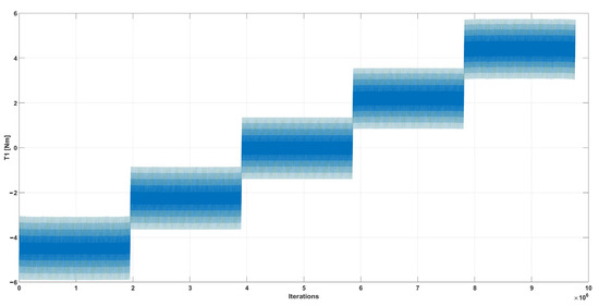
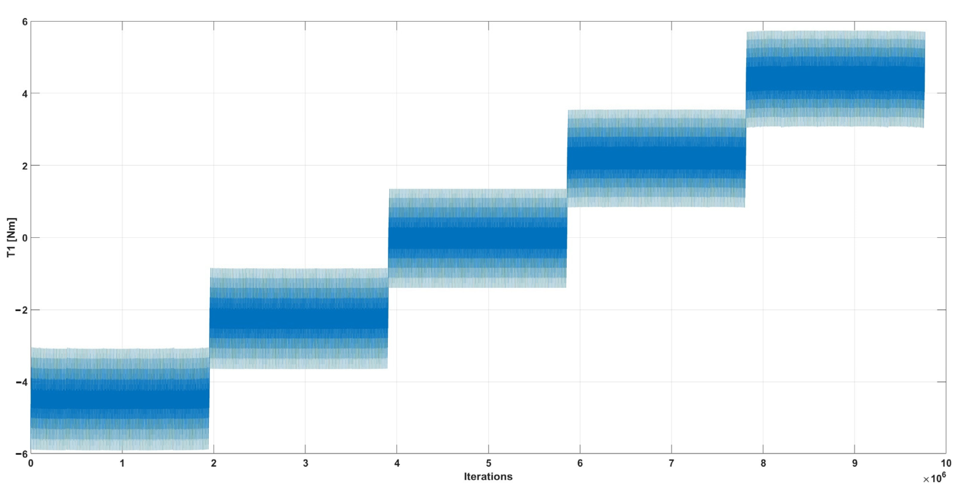
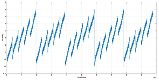
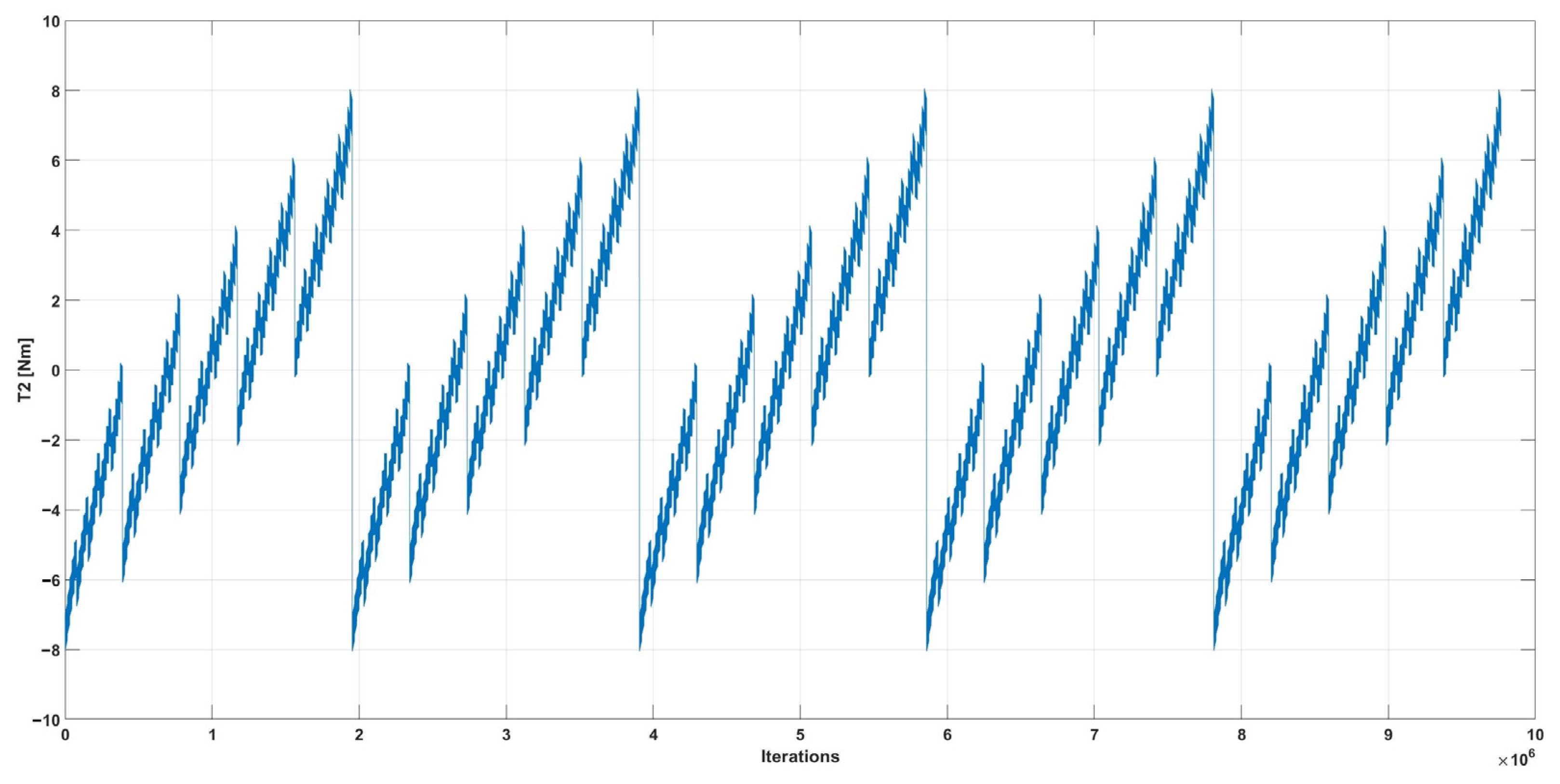
In Figure 13 and Figure 14, the moment induced by gravitational acceleration is shown along the front and side axes. In Appendix A, the equations of T1(1) and T1(2) are used to obtain the pointwise-induced moments for the support pitch joint of the robot. Five different angles are used in each joint of the robot. These joint angles are {−4, −2, 0, 2, 4} degrees. In Figure 13 and Figure 14, the horizontal axis is the number of iterations. To obtain the above results, one joint angle is changed at a time, while the others retain their last-loop values. Here, it is shown that there exists a combination of joint angle values that satisfies the available torque range. In this article, our objective is limited to introducing design principles. Even for static locomotion, it is not an easy task to generate joint trajectories that satisfy the balance of the robot, as well as to stay within the torque limits of the motors. Trajectory generation for a variety of locomotion types is beyond the scope of this article and will be presented in detail in future articles. Also, once the stabilising control system with extroceptive sensor fusion has been thoroughly studied, the results will be included in a separate scientific paper.

Figure 13. The torque induced by gravitational acceleration due to the robot’s joint angle variations in the direction of the frontal axis T_n1.

Figure 14. The torque induced by gravitational acceleration due to the robot’s joint angle variations in the direction of the side axis T_n2.

5. Conclusions and Further Work

RB2 is the second-generation humanoid robot developed at Balikesir University. The design objectives were determined based on our experience with earlier humanoid robots.

The robot was assembled using only two distinct joint structures. This design feature results in a highly modular, interchangeable architecture that simplifies and accelerates the manufacturing process while keeping us within the limited project budget. RB2 was designed to be symmetric along both the sagittal and lateral planes, ensuring structural and functional uniformity without predefined left–right or front–rear orientations. By eliminating mechanical kneecaps, the joint design permits bidirectional flexion within the sagittal plane, offering increased kinematic versatility and enabling novel locomotion strategies in confined spaces.

The second phase of the study involves developing a full three-dimensional nonlinear dynamic model, along with reduced planar dynamic models for simulation and controller design. The multibody dynamic equations will be obtained symbolically using both Lagrange’s and Kane’s methods. In this way, possible modelling errors will be minimised. MATLAB toolboxes will be used to linearize the nonlinear planar models to design initial control systems. It is anticipated that the dynamic modelling and control development phase will demand greater time and effort than the physical design and construction of the entire robotic platform.

Appendix A.1

The moment due to gravity at the support ankle roll joint is shown below in the front axis direction.

$T_1\left(1\right)$ = g*(r5*(cos(t1)*sin(t5) + cos(t2 + t3 + t4)*cos(t5)*sin(t1)) + l1*sin(t1) + l3*cos(t2 + t3)*sin(t1) + l2*cos(t2)*sin(t1) + l4*cos(t2 + t3 + t4)*sin(t1)) + g*(r6*(sin(t6)*(cos(t1)*cos(t5) − cos(t2 + t3 + t4)*sin(t1)*sin(t5)) + cos(t6)*(cos(t1)*sin(t5) + cos(t2 + t3 + t4)*cos(t5)*sin(t1))) + l5*(cos(t1)*sin(t5) + cos(t2 + t3 + t4)*cos(t5)*sin(t1)) + l1*sin(t1) + l3*cos(t2 + t3)*sin(t1) + l2*cos(t2)*sin(t1) + l4*cos(t2 + t3 + t4)*sin(t1)) + g*(r7*(cos(t7)*(sin(t6)*(cos(t1)*cos(t5) − cos(t2 + t3 + t4)*sin(t1)*sin(t5)) + cos(t6)*(cos(t1)*sin(t5) + cos(t2 + t3 + t4)*cos(t5)*sin(t1))) − sin(t2 + t3 + t4)*sin(t1)*sin(t7)) + l6*(sin(t6)*(cos(t1)*cos(t5) − cos(t2 + t3 + t4)*sin(t1)*sin(t5)) + cos(t6)*(cos(t1)*sin(t5) + cos(t2 + t3 + t4)*cos(t5)*sin(t1))) + l5*(cos(t1)*sin(t5) + cos(t2 + t3 + t4)*cos(t5)*sin(t1)) + l1*sin(t1) + l3*cos(t2 + t3)*sin(t1) + l2*cos(t2)*sin(t1) + l4*cos(t2 + t3 + t4)*sin(t1)) + g*(l7*(cos(t1)*cos(t5) − cos(t2 + t3 + t4)*sin(t1)*sin(t5)) − r8*(cos(t8)*(cos(pi)*(cos(t1)*sin(t5) + cos(t2 + t3 + t4)*cos(t5)*sin(t1)) + sin(pi)*(cos(t1)*cos(t5) − cos(t2 + t3 + t4)*sin(t1)*sin(t5))) + sin(t8)*(cos(pi)*(cos(t1)*cos(t5) − cos(t2 + t3 + t4)*sin(t1)*sin(t5)) − sin(pi)*(cos(t1)*sin(t5) + cos(t2 + t3 + t4)*cos(t5)*sin(t1)))) + l1*sin(t1) + l3*cos(t2 + t3)*sin(t1) + l2*cos(t2)*sin(t1) + l4*cos(t2 + t3 + t4)*sin(t1)) − g*(r12*(cos(t12)*(cos(t11)*(cos(t10)*(cos(t9)*(cos(t8)*(cos(pi)*(cos(t1)*sin(t5) + cos(t2 + t3 + t4)*cos(t5)*sin(t1)) + sin(pi)*(cos(t1)*cos(t5) − cos(t2 + t3 + t4)*sin(t1)*sin(t5))) + sin(t8)*(cos(pi)*(cos(t1)*cos(t5) − cos(t2 + t3 + t4)*sin(t1)*sin(t5)) − sin(pi)*(cos(t1)*sin(t5) + cos(t2 + t3 + t4)*cos(t5)*sin(t1)))) − sin(t2 + t3 + t4)*sin(t1)*sin(t9)) − sin(t10)*(sin(t9)*(cos(t8)*(cos(pi)*(cos(t1)*sin(t5) + cos(t2 + t3 + t4)*cos(t5)*sin(t1)) + sin(pi)*(cos(t1)*cos(t5) − cos(t2 + t3 + t4)*sin(t1)*sin(t5))) + sin(t8)*(cos(pi)*(cos(t1)*cos(t5) − cos(t2 + t3 + t4)*sin(t1)*sin(t5)) − sin(pi)*(cos(t1)*sin(t5) + cos(t2 + t3 + t4)*cos(t5)*sin(t1)))) + sin(t2 + t3 + t4)*cos(t9)*sin(t1))) − sin(t11)*(cos(t10)*(sin(t9)*(cos(t8)*(cos(pi)*(cos(t1)*sin(t5) + cos(t2 + t3 + t4)*cos(t5)*sin(t1)) + sin(pi)*(cos(t1)*cos(t5) − cos(t2 + t3 + t4)*sin(t1)*sin(t5))) + sin(t8)*(cos(pi)*(cos(t1)*cos(t5) − cos(t2 + t3 + t4)*sin(t1)*sin(t5)) − sin(pi)*(cos(t1)*sin(t5) + cos(t2 + t3 + t4)*cos(t5)*sin(t1)))) + sin(t2 + t3 + t4)*cos(t9)*sin(t1)) + sin(t10)*(cos(t9)*(cos(t8)*(cos(pi)*(cos(t1)*sin(t5) + cos(t2 + t3 + t4)*cos(t5)*sin(t1)) + sin(pi)*(cos(t1)*cos(t5) − cos(t2 + t3 + t4)*sin(t1)*sin(t5))) + sin(t8)*(cos(pi)*(cos(t1)*cos(t5) − cos(t2 + t3 + t4)*sin(t1)*sin(t5)) − sin(pi)*(cos(t1)*sin(t5) + cos(t2 + t3 + t4)*cos(t5)*sin(t1)))) − sin(t2 + t3 + t4)*sin(t1)*sin(t9)))) + sin(t12)*(cos(t8)*(cos(pi)*(cos(t1)*cos(t5) − cos(t2 + t3 + t4)*sin(t1)*sin(t5)) − sin(pi)*(cos(t1)*sin(t5) + cos(t2 + t3 + t4)*cos(t5)*sin(t1))) − sin(t8)*(cos(pi)*(cos(t1)*sin(t5) + cos(t2 + t3 + t4)*cos(t5)*sin(t1)) + sin(pi)*(cos(t1)*cos(t5) − cos(t2 + t3 + t4)*sin(t1)*sin(t5))))) + l3*(cos(t9)*(cos(t8)*(cos(pi)*(cos(t1)*sin(t5) + cos(t2 + t3 + t4)*cos(t5)*sin(t1)) + sin(pi)*(cos(t1)*cos(t5) − cos(t2 + t3 + t4)*sin(t1)*sin(t5))) + sin(t8)*(cos(pi)*(cos(t1)*cos(t5) − cos(t2 + t3 + t4)*sin(t1)*sin(t5)) − sin(pi)*(cos(t1)*sin(t5) + cos(t2 + t3 + t4)*cos(t5)*sin(t1)))) − sin(t2 + t3 + t4)*sin(t1)*sin(t9)) + l4*(cos(t8)*(cos(pi)*(cos(t1)*sin(t5) + cos(t2 + t3 + t4)*cos(t5)*sin(t1)) + sin(pi)*(cos(t1)*cos(t5) − cos(t2 + t3 + t4)*sin(t1)*sin(t5))) + sin(t8)*(cos(pi)*(cos(t1)*cos(t5) − cos(t2 + t3 + t4)*sin(t1)*sin(t5)) − sin(pi)*(cos(t1)*sin(t5) + cos(t2 + t3 + t4)*cos(t5)*sin(t1)))) + l1*(cos(t10)*(cos(t9)*(cos(t8)*(cos(pi)*(cos(t1)*sin(t5) + cos(t2 + t3 + t4)*cos(t5)*sin(t1)) + sin(pi)*(cos(t1)*cos(t5) − cos(t2 + t3 + t4)*sin(t1)*sin(t5))) + sin(t8)*(cos(pi)*(cos(t1)*cos(t5) − cos(t2 + t3 + t4)*sin(t1)*sin(t5)) − sin(pi)*(cos(t1)*sin(t5) + cos(t2 + t3 + t4)*cos(t5)*sin(t1)))) − sin(t2 + t3 + t4)*sin(t1)*sin(t9)) − sin(t10)*(sin(t9)*(cos(t8)*(cos(pi)*(cos(t1)*sin(t5) + cos(t2 + t3 + t4)*cos(t5)*sin(t1)) + sin(pi)*(cos(t1)*cos(t5) − cos(t2 + t3 + t4)*sin(t1)*sin(t5))) + sin(t8)*(cos(pi)*(cos(t1)*cos(t5) − cos(t2 + t3 + t4)*sin(t1)*sin(t5)) − sin(pi)*(cos(t1)*sin(t5) + cos(t2 + t3 + t4)*cos(t5)*sin(t1)))) + sin(t2 + t3 + t4)*cos(t9)*sin(t1))) + l2*(cos(t10)*(cos(t9)*(cos(t8)*(cos(pi)*(cos(t1)*sin(t5) + cos(t2 + t3 + t4)*cos(t5)*sin(t1)) + sin(pi)*(cos(t1)*cos(t5) − cos(t2 + t3 + t4)*sin(t1)*sin(t5))) + sin(t8)*(cos(pi)*(cos(t1)*cos(t5) − cos(t2 + t3 + t4)*sin(t1)*sin(t5)) − sin(pi)*(cos(t1)*sin(t5) + cos(t2 + t3 + t4)*cos(t5)*sin(t1)))) − sin(t2 + t3 + t4)*sin(t1)*sin(t9)) − sin(t10)*(sin(t9)*(cos(t8)*(cos(pi)*(cos(t1)*sin(t5) + cos(t2 + t3 + t4)*cos(t5)*sin(t1)) + sin(\pi)*(cos(t1)*cos(t5) − cos(t2 + t3 + t4)*sin(t1)*sin(t5))) + sin(t8)*(cos(pi)*(cos(t1)*cos(t5) − cos(t2 + t3 + t4)*sin(t1)*sin(t5)) − sin(pi)*(cos(t1)*sin(t5) + cos(t2 + t3 + t4)*cos(t5)*sin(t1)))) + sin(t2 + t3 + t4)*cos(t9)*sin(t1))) − l7*(cos(t1)*cos(t5) − cos(t2 + t3 + t4)*sin(t1)*sin(t5)) − l1*sin(t1) − l3*cos(t2 + t3)*sin(t1) − l2*cos(t2)*sin(t1) − l4*cos(t2 + t3 + t4)*sin(t1)) + g*(l1*sin(t1) + r2*cos(t2)*sin(t1)) + g*(l7*(cos(t1)*cos(t5) − cos(t2 + t3 + t4)*sin(t1)*sin(t5)) − l4*(cos(t8)*(cos(pi)*(cos(t1)*sin(t5) + cos(t2 + t3 + t4)*cos(t5)*sin(t1)) + sin(pi)*(cos(t1)*cos(t5) − cos(t2 + t3 + t4)*sin(t1)*sin(t5))) + sin(t8)*(cos(pi)*(cos(t1)*cos(t5) − cos(t2 + t3 + t4)*sin(t1)*sin(t5)) − sin(pi)*(cos(t1)*sin(t5) + cos(t2 + t3 + t4)*cos(t5)*sin(t1)))) − r9*(cos(t9)*(cos(t8)*(cos(pi)*(cos(t1)*sin(t5) + cos(t2 + t3 + t4)*cos(t5)*sin(t1)) + sin(pi)*(cos(t1)*cos(t5) − cos(t2 + t3 + t4)*sin(t1)*sin(t5))) + sin(t8)*(cos(pi)*(cos(t1)*cos(t5) − cos(t2 + t3 + t4)*sin(t1)*sin(t5)) − sin(pi)*(cos(t1)*sin(t5) + cos(t2 + t3 + t4)*cos(t5)*sin(t1)))) − sin(t2 + t3 + t4)*sin(t1)*sin(t9)) + l1*sin(t1) + l3*cos(t2 + t3)*sin(t1) + l2*cos(t2)*sin(t1) + l4*cos(t2 + t3 + t4)*sin(t1)) + g*(l1*sin(t1) + l3*cos(t2 + t3)*sin(t1) + l2*cos(t2)*sin(t1) + r4*cos(t2 + t3 + t4)*sin(t1)) + g*(l7*(cos(t1)*cos(t5) − cos(t2 + t3 + t4)*sin(t1)*sin(t5)) − l4*(cos(t8)*(cos(pi)*(cos(t1)*sin(t5) + cos(t2 + t3 + t4)*cos(t5)*sin(t1)) + sin(pi)*(cos(t1)*cos(t5) − cos(t2 + t3 + t4)*sin(t1)*sin(t5))) + sin(t8)*(cos(pi)*(cos(t1)*cos(t5) − cos(t2 + t3 + t4)*sin(t1)*sin(t5)) − sin(pi)*(cos(t1)*sin(t5) + cos(t2 + t3 + t4)*cos(t5)*sin(t1)))) − l2*(cos(t10)*(cos(t9)*(cos(t8)*(cos(pi)*(cos(t1)*sin(t5) + cos(t2 + t3 + t4)*cos(t5)*sin(t1)) + sin(pi)*(cos(t1)*cos(t5) − cos(t2 + t3 + t4)*sin(t1)*sin(t5))) + sin(t8)*(cos(pi)*(cos(t1)*cos(t5) − cos(t2 + t3 + t4)*sin(t1)*sin(t5)) − sin(pi)*(cos(t1)*sin(t5) + cos(t2 + t3 + t4)*cos(t5)*sin(t1)))) − sin(t2 + t3 + t4)*sin(t1)*sin(t9)) − sin(t10)*(sin(t9)*(cos(t8)*(cos(pi)*(cos(t1)*sin(t5) + cos(t2 + t3 + t4)*cos(t5)*sin(t1)) + sin(pi)*(cos(t1)*cos(t5) − cos(t2 + t3 + t4)*sin(t1)*sin(t5))) + sin(t8)*(cos(pi)*(cos(t1)*cos(t5) − cos(t2 + t3 + t4)*sin(t1)*sin(t5)) − sin(pi)*(cos(t1)*sin(t5) + cos(t2 + t3 + t4)*cos(t5)*sin(t1)))) + sin(t2 + t3 + t4)*cos(t9)*sin(t1))) − l3*(cos(t9)*(cos(t8)*(cos(pi)*(cos(t1)*sin(t5) + cos(t2 + t3 + t4)*cos(t5)*sin(t1)) + sin(pi)*(cos(t1)*cos(t5) − cos(t2 + t3 + t4)*sin(t1)*sin(t5))) + sin(t8)*(cos(pi)*(cos(t1)*cos(t5) − cos(t2 + t3 + t4)*sin(t1)*sin(t5)) − sin(pi)*(cos(t1)*sin(t5) + cos(t2 + t3 + t4)*cos(t5)*sin(t1)))) − sin(t2 + t3 + t4)*sin(t1)*sin(t9)) + l1*sin(t1) − r11*(cos(t11)*(cos(t10)*(cos(t9)*(cos(t8)*(cos(pi)*(cos(t1)*sin(t5) + cos(t2 + t3 + t4)*cos(t5)*sin(t1)) + sin(pi)*(cos(t1)*cos(t5) − cos(t2 + t3 + t4)*sin(t1)*sin(t5))) + sin(t8)*(cos(pi)*(cos(t1)*cos(t5) − cos(t2 + t3 + t4)*sin(t1)*sin(t5)) − sin(pi)*(cos(t1)*sin(t5) + cos(t2 + t3 + t4)*cos(t5)*sin(t1)))) − sin(t2 + t3 + t4)*sin(t1)*sin(t9)) − sin(t10)*(sin(t9)*(cos(t8)*(cos(pi)*(cos(t1)*sin(t5) + cos(t2 + t3 + t4)*cos(t5)*sin(t1)) + sin(pi)*(cos(t1)*cos(t5) − cos(t2 + t3 + t4)*sin(t1)*sin(t5))) + sin(t8)*(cos(pi)*(cos(t1)*cos(t5) − cos(t2 + t3 + t4)*sin(t1)*sin(t5)) − sin(pi)*(cos(t1)*sin(t5) + cos(t2 + t3 + t4)*cos(t5)*sin(t1)))) + sin(t2 + t3 + t4)*cos(t9)*sin(t1))) − sin(t11)*(cos(t10)*(sin(t9)*(cos(t8)*(cos(pi)*(cos(t1)*sin(t5) + cos(t2 + t3 + t4)*cos(t5)*sin(t1)) + sin(pi)*(cos(t1)*cos(t5) − cos(t2 + t3 + t4)*sin(t1)*sin(t5))) + sin(t8)*(cos(pi)*(cos(t1)*cos(t5) − cos(t2 + t3 + t4)*sin(t1)*sin(t5)) − sin(pi)*(cos(t1)*sin(t5) + cos(t2 + t3 + t4)*cos(t5)*sin(t1)))) + sin(t2 + t3 + t4)*cos(t9)*sin(t1)) + sin(t10)*(cos(t9)*(cos(t8)*(cos(pi)*(cos(t1)*sin(t5) + cos(t2 + t3 + t4)*cos(t5)*sin(t1)) + sin(pi)*(cos(t1)*cos(t5) − cos(t2 + t3 + t4)*sin(t1)*sin(t5))) + sin(t8)*(cos(pi)*(cos(t1)*cos(t5) − cos(t2 + t3 + t4)*sin(t1)*sin(t5)) − sin(pi)*(cos(t1)*sin(t5) + cos(t2 + t3 + t4)*cos(t5)*sin(t1)))) − sin(t2 + t3 + t4)*sin(t1)*sin(t9)))) + l3*cos(t2 + t3)*sin(t1) + l2*cos(t2)*sin(t1) + l4*cos(t2 + t3 + t4)*sin(t1)) + g*(l1*sin(t1) + r3*cos(t2 + t3)*sin(t1) + l2*cos(t2)*sin(t1)) + g*(l7*(cos(t1)*cos(t5) − cos(t2 + t3 + t4)*sin(t1)*sin(t5)) − l4*(cos(t8)*(cos(pi)*(cos(t1)*sin(t5) + cos(t2 + t3 + t4)*cos(t5)*sin(t1)) + sin(pi)*(cos(t1)*cos(t5) − cos(t2 + t3 + t4)*sin(t1)*sin(t5))) + sin(t8)*(cos(pi)*(cos(t1)*cos(t5) − cos(t2 + t3 + t4)*sin(t1)*sin(t5)) − sin(pi)*(cos(t1)*sin(t5) + cos(t2 + t3 + t4)*cos(t5)*sin(t1)))) − r10*(cos(t10)*(cos(t9)*(cos(t8)*(cos(pi)*(cos(t1)*sin(t5) + cos(t2 + t3 + t4)*cos(t5)*sin(t1)) + sin(pi)*(cos(t1)*cos(t5) − cos(t2 + t3 + t4)*sin(t1)*sin(t5))) + sin(t8)*(cos(pi)*(cos(t1)*cos(t5) − cos(t2 + t3 + t4)*sin(t1)*sin(t5)) − sin(pi)*(cos(t1)*sin(t5) + cos(t2 + t3 + t4)*cos(t5)*sin(t1)))) − sin(t2 + t3 + t4)*sin(t1)*sin(t9)) − sin(t10)*(sin(t9)*(cos(t8)*(cos(pi)*(cos(t1)*sin(t5) + cos(t2 + t3 + t4)*cos(t5)*sin(t1)) + sin(pi)*(cos(t1)*cos(t5) − cos(t2 + t3 + t4)*sin(t1)*sin(t5))) + sin(t8)*(cos(pi)*(cos(t1)*cos(t5) − cos(t2 + t3 + t4)*sin(t1)*sin(t5)) − sin(pi)*(cos(t1)*sin(t5) + cos(t2 + t3 + t4)*cos(t5)*sin(t1)))) + sin(t2 + t3 + t4)*cos(t9)*sin(t1))) − l3*(cos(t9)*(cos(t8)*(cos(pi)*(cos(t1)*sin(t5) + cos(t2 + t3 + t4)*cos(t5)*sin(t1)) + sin(pi)*(cos(t1)*cos(t5) − cos(t2 + t3 + t4)*sin(t1)*sin(t5))) + sin(t8)*(cos(pi)*(cos(t1)*cos(t5) − cos(t2 + t3 + t4)*sin(t1)*sin(t5)) − sin(pi)*(cos(t1)*sin(t5) + cos(t2 + t3 + t4)*cos(t5)*sin(t1)))) − sin(t2 + t3 + t4)*sin(t1)*sin(t9)) + l1*sin(t1) + l3*cos(t2 + t3)*sin(t1) + l2*cos(t2)*sin(t1) + l4*cos(t2 + t3 + t4)*sin(t1)) + g*r1*sin(t1);

Appendix A.2

The moment due to gravity at the support ankle roll joint is shown below in the side axis direction.

$T_1\left(2\right)$ = g*(l3*sin(t2 + t3) + l2*sin(t2) + l4*sin(t2 + t3 + t4) + r5*sin(t2 + t3 + t4)*cos(t5)) − g*(l3*(cos(t2 + t3 + t4)*sin(t9) + cos(pi + t5 + t8)*sin(t2 + t3 + t4)*cos(t9)) + l2*(cos(t10)*(cos(t2 + t3 + t4)*sin(t9) + cos(pi + t5 + t8)*sin(t2 + t3 + t4)*cos(t9)) + sin(t10)*(cos(t2 + t3 + t4)*cos(t9) − cos(pi + t5 + t8)*sin(t2 + t3 + t4)*sin(t9))) + r11*(cos(t11)*(cos(t10)*(cos(t2 + t3 + t4)*sin(t9) + cos(pi + t5 + t8)*sin(t2 + t3 + t4)*cos(t9)) + sin(t10)*(cos(t2 + t3 + t4)*cos(t9) − cos(pi + t5 + t8)*sin(t2 + t3 + t4)*sin(t9))) + sin(t11)*(cos(t10)*(cos(t2 + t3 + t4)*cos(t9) − cos(pi + t5 + t8)*sin(t2 + t3 + t4)*sin(t9)) − sin(t10)*(cos(t2 + t3 + t4)*sin(t9) + cos(pi + t5 + t8)*sin(t2 + t3 + t4)*cos(t9)))) − l3*sin(t2 + t3) − l2*sin(t2) − l4*sin(t2 + t3 + t4) + l4*cos(pi + t5 + t8)*sin(t2 + t3 + t4) + l7*sin(t2 + t3 + t4)*sin(t5)) + g*(l3*sin(t2 + t3) + l2*sin(t2) + l4*sin(t2 + t3 + t4) − r8*cos(pi + t5 + t8)*sin(t2 + t3 + t4) − l7*sin(t2 + t3 + t4)*sin(t5)) + g*(r4*sin(t2 + t3 + t4) + l3*sin(t2 + t3) + l2*sin(t2)) − g*(r9*(cos(t2 + t3 + t4)*sin(t9) + cos(pi + t5 + t8)*sin(t2 + t3 + t4)*cos(t9)) − l3*sin(t2 + t3) − l2*sin(t2) − l4*sin(t2 + t3 + t4) + l4*cos(pi + t5 + t8)*sin(t2 + t3 + t4) + l7*sin(t2 + t3 + t4)*sin(t5)) − g*(l3*(cos(t2 + t3 + t4)*sin(t9) + cos(pi + t5 + t8)*sin(t2 + t3 + t4)*cos(t9)) + l1*(cos(t10)*(cos(t2 + t3 + t4)*sin(t9) + cos(pi + t5 + t8)*sin(t2 + t3 + t4)*cos(t9)) + sin(t10)*(cos(t2 + t3 + t4)*cos(t9) − cos(pi + t5 + t8)*sin(t2 + t3 + t4)*sin(t9))) + l2*(cos(t10)*(cos(t2 + t3 + t4)*sin(t9) + cos(pi + t5 + t8)*sin(t2 + t3 + t4)*cos(t9)) + sin(t10)*(cos(t2 + t3 + t4)*cos(t9) − cos(pi + t5 + t8)*sin(t2 + t3 + t4)*sin(t9))) − l3*sin(t2 + t3) + r12*(cos(t12)*(cos(t11)*(cos(t10)*(cos(t2 + t3 + t4)*sin(t9) + cos(pi + t5 + t8)*sin(t2 + t3 + t4)*cos(t9)) + sin(t10)*(cos(t2 + t3 + t4)*cos(t9) − cos(pi + t5 + t8)*sin(t2 + t3 + t4)*sin(t9))) + sin(t11)*(cos(t10)*(cos(t2 + t3 + t4)*cos(t9) − cos(pi + t5 + t8)*sin(t2 + t3 + t4)*sin(t9)) − sin(t10)*(cos(t2 + t3 + t4)*sin(t9) + cos(pi + t5 + t8)*sin(t2 + t3 + t4)*cos(t9)))) − sin(pi + t5 + t8)*sin(t2 + t3 + t4)*sin(t12)) − l2*sin(t2) − l4*sin(t2 + t3 + t4) + l4*cos(pi + t5 + t8)*sin(t2 + t3 + t4) + l7*sin(t2 + t3 + t4)*sin(t5)) + g*(r3*sin(t2 + t3) + l2*sin(t2)) + g*(l3*sin(t2 + t3) + r7*(cos(t2 + t3 + t4)*sin(t7) + sin(t2 + t3 + t4)*cos(t5 + t6)*cos(t7)) + l2*sin(t2) + l4*sin(t2 + t3 + t4) + l6*sin(t2 + t3 + t4)*cos(t5 + t6) + l5*sin(t2 + t3 + t4)*cos(t5)) − g*(l3*(cos(t2 + t3 + t4)*sin(t9) + cos(pi + t5 + t8)*sin(t2 + t3 + t4)*cos(t9)) + r10*(cos(t10)*(cos(t2 + t3 + t4)*sin(t9) + cos(pi + t5 + t8)*sin(t2 + t3 + t4)*cos(t9)) + sin(t10)*(cos(t2 + t3 + t4)*cos(t9) − cos(pi + t5 + t8)*sin(t2 + t3 + t4)*sin(t9))) − l3*sin(t2 + t3) − l2*sin(t2) − l4*sin(t2 + t3 + t4) + l4*cos(pi + t5 + t8)*sin(t2 + t3 + t4) + l7*sin(t2 + t3 + t4)*sin(t5)) + g*(l3*sin(t2 + t3) + l2*sin(t2) + l4*sin(t2 + t3 + t4) + r6*sin(t2 + t3 + t4)*cos(t5 + t6) + l5*sin(t2 + t3 + t4)*cos(t5)) + g*r2*sin(t2);

References

- Parmiggiani, A.; Maggiali, M.; Natale, L.; Nori, F.; Schmitz, A.; Tsagarakis, N.; Victor, J.S.; Becchi, F.; Sandini, G.; Metta, G. The design of the iCub humanoid robot. Int. J. Humanoid Robot. 2012, 9, 1250027. [Google Scholar] [CrossRef] [Scilit]
- Takanishi, A. Historical Perspective of Humanoid Robot Research in Asia. In Humanoid Robotics: A Reference; Goswami, A., Vadakkepat, P., Eds.; Springer: Dordrecht, The Netherlands, 2019. [Google Scholar] [CrossRef] [Scilit]
- Schaal, S. Historical Perspective of Humanoid Robot Research in the Americas. In Humanoid Robotics: A Reference; Goswami, A., Vadakkepat, P., Eds.; Springer: Dordrecht, The Netherlands, 2018. [Google Scholar] [CrossRef] [Scilit]
- Hirose, M.; Ogawa, K. Honda humanoid robots development. Philos. Trans. R. Soc. A Math. Phys. Eng. Sci. 2007, 365, 11–19. [Google Scholar] [CrossRef] [Scilit] [PubMed]
- LimX Dynamics. Oli—Full-Size General-Purpose Humanoid Robot. Available online: https://www.limxdynamics.com/en/products/oli (accessed on 28 March 2026).
- ENGINEAI. Available online: https://en.engineai.com.cn/ (accessed on 28 March 2026).
- PENG Motors. XPENG Shares Achievements in Physical AI Emergence: Unveils XPENG VLA 2.0, Robotaxi, Next-Gen IRON, and Flying Car. XPENG Official Newsroom. 5 November 2025. Available online: https://www.xpeng.com/news/019a56f54fe99a2a0a8d8a0282e402b7 (accessed on 28 March 2026).
- Phybot Technology Co., Ltd. PHYBOT M1. Available online: https://www.phybot.tech/phybot-m1 (accessed on 28 March 2026).
- Figure AI. Introducing Figure 03. 9 October 2025. Available online: https://www.figure.ai/news/introducing-figure-03 (accessed on 28 March 2026).
- Boston Dynamics. Atlas Humanoid Robot. Available online: https://bostondynamics.com/atlas/ (accessed on 28 March 2026).
- Agile Robots SE. We Are Agile Robots: Driving Industries Forward. Available online: https://www.agile-robots.com/en/ (accessed on 28 March 2026).
- Unitree Robotics. Unitree H2 Destiny Awakening. Available online: https://www.unitree.com/H2 (accessed on 28 March 2026).
- DEEP Robotics. DR02—A New-Generation Industrial-Level Humanoid Robot. Available online: https://www.deeprobotics.cn/en/index/dr02.html (accessed on 28 March 2026).
- Sheng, Q.; Zhou, Z.; Li, J.; Mi, X.; Xiang, P.; Chen, Z.; Xu, H.; Jia, S.; Wu, X.; Cui, Y.; et al. A comprehensive review of humanoid robots. SmartBot 2025, 1, e12008. [Google Scholar] [CrossRef] [Scilit]
- Dario, P.; Guglielmelli, E.; Laschi, C. Humanoids and Personal Robots: Design and Experiments. J. Robot. Syst. 2001, 18, 673–690. [Google Scholar] [CrossRef] [Scilit]
- Hirai, K.; Hirose, M.; Haikawa, Y.; Takenaka, T. The Development of Honda Humanoid Robot. In Proceedings of the 1998 IEEE International Conference on Robotics and Automation, Leuven, Belgium, 20 May 1998. [Google Scholar]
- Kaneko, K.; Kajita, S.; Yokoi, K.; Hugel, V.; Blazevic, P.; Coiffet, P. Design of LRP Humanoid Robot and Its Control Method. In Proceedings of the 10th IEEE International Workshop on Robot and Human Interactive Communication (ROMAN 2001), Bordeaux and Paris, France, 18–21 September 2001. [Google Scholar]
- Nishiwaki, K.; Kuffner, J.; Kagami, S.; Inaba, M.; Inoue, H. The Experimental Humanoid Robot H7: A Research Platform for Autonomous Behaviour. Philos. Trans. R. Soc. A Math. Phys. Eng. Sci. 2007, 365, 79–107. [Google Scholar] [CrossRef] [Scilit] [PubMed]
- Kojima, K.; Karasawa, T.; Kozuki, T.; Kuroiwa, E.; Yukizaki, S.; Iwaishi, S.; Ishikawa, T.; Koyama, R.; Noda, S.; Sugai, F.; et al. Development of Life-Sized High-Power Humanoid Robot JAXON for Real-World Use. In Proceedings of the 2015 IEEE-RAS 15th International Conference on Humanoid Robots (Humanoids), Seoul, Republic of Korea, 3–5 November 2015. [Google Scholar]
- Hyon, S.H.; Suewaka, D.; Torii, Y.; Oku, N. Design and Experimental Evaluation of a Fast Torque-Controlled Hydraulic Humanoid Robot. IEEE/ASME Trans. Mechatron. 2017, 22, 623–634. [Google Scholar] [CrossRef] [Scilit]
- Kazuhito, K.; Kanehiro, F.; Morisawa, M.; Akachi, K.; Miyamori, G.; Hayashi, A.; Kanehira, N. Humanoid Robot HRP-4—Humanoid Robotics Platform with Lightweight and Slim Body. In Proceedings of the 2011 IEEE/RSJ International Conference on Intelligent Robots and Systems, San Francisco, CA, USA, 25–30 September 2011. [Google Scholar]
- Kaneko, K.; Kaminaga, H.; Sakaguchi, T.; Kajita, S.; Morisawa, M.; Kumagai, I.; Kanehiro, F. Humanoid Robot HRP-5P: An Electrically Actuated Humanoid Robot with High-Power and Wide-Range Joints. IEEE Robot. Autom. Lett. 2019, 4, 1431–1438. [Google Scholar] [CrossRef] [Scilit]
- Buschmann, T.; Lohmeier, S.; Ulbrich, H. Humanoid robot lola: Design and walking control. J. Physiol. 2009, 103, 141–148. [Google Scholar] [CrossRef] [Scilit] [PubMed]
- Eßer, J.; Kumar, S.; Peters, H.; Bargsten, V.; de Gea Fernandez, J.; Mastalli, C.; Stasse, O.; Kirchner, F. Design, Analysis and Control of the Series-Parallel Hybrid RH5 Humanoid Robot. In Proceedings of the 2020 IEEE-RAS 20th International Conference on Humanoid Robots (Humanoids), Virtual, 19–21 July 2021. [Google Scholar]
- Humanoid Robot Adam. Available online: https://www.pndbotics.com/humanoid (accessed on 28 March 2026).
- Kanehira, N.; Kawasaki, T.U.; Ohta, S.; Ismumi, T.; Kawada, T.; Kanehiro, F.; Kajita, S.; Kaneko, K. Design and experiments of advanced leg module (HRP-2L) for humanoid robot (HRP-2) development. In Proceedings of the IEEE/RSJ International Conference on Intelligent Robots and Systems, Lausanne, Switzerland, 30 September–4 October 2002. [Google Scholar]
- Lim, H.O.; Takanishi, A. Biped Walking Robots Created at Waseda University: WL and WABIAN Family. Philos. Trans. R. Soc. A Math. Phys. Eng. Sci. 2007, 365, 49–64. [Google Scholar] [CrossRef] [Scilit] [PubMed]
- Steve, D.; Caldwell, D.G. Biologically Inspired Damage Tolerance in Braided Pneumatic Muscle Actuators. J. Intell. Mater. Syst. Struct. 2012, 23, 313–325. [Google Scholar]
- Li, X.; Yu, H.; Feng, H.; Zhang, S.; Fu, Y. Design and Control for WLR-3P: A Hydraulic Wheel-Legged Robot. Cyborg Bionics Syst. 2023, 4, 25. [Google Scholar] [CrossRef] [Scilit] [PubMed]
- Radford, N.A.; Strawser, P.; Hambuchen, K.; Mehling, J.S.; Verdeyen, W.K.; Donnan, A.S.; Holley, J.; Sanchez, J.; Nguyen, V.; Bridgwater, L.; et al. Valkyrie: NASA’s First Bipedal Humanoid Robot. J. Field Robot. 2015, 32, 397–419. [Google Scholar] [CrossRef] [Scilit]
- Xia, Z.; Liu, L.; Xiong, J.; Yi, Q.; Chen, K. Design Aspects and Development of Humanoid Robot THBIP-2. Robotica 2008, 26, 109–116. [Google Scholar] [CrossRef] [Scilit]
- Vukobratovic, M.; Potkonjak, V.; Tzafestas, S. Human and Humanoid Dynamics. J. Intell. Robot. Syst. 2004, 41, 65–84. [Google Scholar] [CrossRef] [Scilit]
- Ulbrich, H.; Buschmann, T.; Lohmeier, S. Development of the Humanoid Robot LOLA. Appl. Mech. Mater. 2006, 5–6, 529–540. [Google Scholar] [CrossRef]
- Akdas, D.; Medrano-Cerda, G.A. Design of a Stabilizing Controller for a Ten-Degree-of-Freedom Bipedal Robot Using Linear Quadratic Regulator Theory. Proc. Inst. Mech. Eng. Part C J. Mech. Eng. Sci. 2001, 215, 27–43. [Google Scholar] [CrossRef] [Scilit]
- Akdas, D. An Effective Mechanical Design and Realization of a Humanoid Robot BUrobot. Acta Polytech. Hung. 2014, 11, 115–134. [Google Scholar] [CrossRef] [Scilit]
- Shinsuke, S.; Konno, A.; Uchiyama, M. Design and Evaluation of a Gravity Compensation Mechanism for a Humanoid Robot. In Proceedings of the 2007 IEEE/RSJ International Conference on Intelligent Robots and Systems, San Diego, CA, USA, 29 October–2 November 2007. [Google Scholar]
- Shabana, A.A. Dynamics of Multibody Systems; Cambridge University Press: Cambridge, UK, 2020; ISBN 978-1108485647. [Google Scholar]
- Yamamoto, K. Human-Like Toe Joint Mechanism. In Humanoid Robotics: A Reference; Springer: Dordrecht, The Netherlands, 2019; pp. 435–456. [Google Scholar]
- Gouaillier, D.; Hugel, V.; Blazevic, P.; Kilner, C.; Monceaux, J.; Lafourcade, P.; Marnier, B.; Serre, J.; Maisonnier, B. Mechatronic design of NAO humanoid. In Proceedings of the 2009 IEEE International Conference on Robotics and Automation, Kobe, Japan, 12–17 May 2009. [Google Scholar]
- SOLIDWORKS. Available online: https://www.solidworks.com/ (accessed on 28 March 2026).
- Liang, C.; Ceccarelli, M. Design and Simulation of a Waist–Trunk System for a Humanoid Robot. Mech. Mach. Theory 2012, 53, 50–65. [Google Scholar] [CrossRef] [Scilit]
- Hern, C.; Soto, R.; Rodriguez, E. Design and Dynamic Modeling of Humanoid Biped Robot E-Robot. In Proceedings of the 2011 IEEE Electronics, Robotics and Automotive Mechanics Conference, Cuernavaca, Mexico, 15–18 November 2011. [Google Scholar]
- Engineai T800. Available online: https://en.engineai.com.cn/product-t800.html (accessed on 28 March 2026).
- Hamill, J.; Knutzen, K.M. Biomechanical Basis of Human Movement, 4th ed.; Lippincott Williams & Wilkins: Philadelphia, PA, USA, 2006; pp. 402–410. [Google Scholar]
- Mu, Y.; Wang, S.; Guo, A.; Qu, P.; Han, W.; Yan, Q.; Liu, H.; Liu, C. Design and Gait Simulation Study of Wheel-Legged Conversion Device Used in Hexapod Bionic Robot. Processes 2025, 13, 3364. [Google Scholar] [CrossRef] [Scilit]
Disclaimer/Publisher’s Note: The statements, opinions and data contained in all publications are solely those of the individual author(s) and contributor(s) and not of MDPI and/or the editor(s). MDPI and/or the editor(s) disclaim responsibility for any injury to people or property resulting from any ideas, methods, instructions or products referred to in the content. |
© 2026 by the author. Licensee MDPI, Basel, Switzerland. This article is an open access article distributed under the terms and conditions of the Creative Commons Attribution (CC BY) license.