Development of a Preliminary Renewable Energy Planning Tool with Storage and Carbon Footprint Assessment

Abstract

The global transition toward a low-carbon economy has accelerated the adoption of renewable energy sources. This paper presents the development of a model-based electronic Decision Support System for renewable energy planning, incorporating energy storage and carbon footprint assessment. The tool assists stakeholders in the preliminary evaluation of local wind and solar resources. To validate the model’s credibility, a comparative analysis was conducted, using the Port of Sines, Portugal, as an industrial case study. Solar energy estimations were benchmarked against PVSyst, while wind energy simulations were compared with an INEGI technical study. Results indicate consistency in solar estimates, with maximum deviations of 14% for fixed installations and 13% for vertical barriers, primarily due to terrain orography that was not yet integrated into the algorithm. Regarding wind energy, deviations reached 19% to 25%, largely resulting from the use of aggregated mean values in the reference data and generic turbine models. Overall, this work contributes to energy engineering by formalizing a validated workflow that facilitates early-stage sizing and strategic investment decisions under conditions of data scarcity. The tool proves effective for rapid screening of promising investment options while maintaining a balance between computational complexity and practical usability.

1. Introduction

As the use of renewable systems continues to grow, there is an increasing demand for simulation tools that predict system performance and profitability. In the photovoltaic energy sector, there is a wide array of simulation tools and software already available, spanning from basic to advanced solutions, including Photovoltaic Geographical Information System (PVGIS), PVSyst, PVWatts, SolarGIS, or PVSOL, for example [1].

There are several key criteria for evaluating the effectiveness of solar simulation software, namely the software cost and availability, solar databases, working platforms, frequency of updates, reporting and analysis options, flexibility of simulation data requirement, energy and economic and environmental modeling capabilities, and finally, the user friendliness and ease of use [2].

For wind energy simulations, there is also a wide range of simulation programs, such as Wind Atlas Analysis and Application Program (WAsP), WindPro, WindFarmer, WindSim, Meteodyn, HOMER, or RETScreen. The last two programs use linear methods, while WAsP, WindPro, and WindFarmer are based on flow-field modeling. WindSim and Meteodyn, in turn, use computational fluid dynamics, a nonlinear method [3].

The difference between linear and non-linear models is that the former relies on historical meteorological measurement data. In contrast, tools based on non-linear methods consider terrain topography and roughness, and for weather forecasting, they use meteorological data from Numerical Weather Prediction (NWP) models [4]. Given that the wind is a highly unpredictable weather variable, the accuracy of wind energy prediction depends on several factors, including the availability of wind speed data at the reference station, the correlation between the meteorological data of the target and reference stations, the time scale, and the type of software adopted [5].

In parallel with these developments in renewable energy forecasting, the ability to simulate an entity’s carbon footprint has become increasingly important. Such simulations make it possible to estimate emissions associated with past or future activities and to devise scenarios that assess the impact of implementing environmental measures [6]. Currently, in the maritime sector, there are several platforms available on the market that estimate carbon footprint, taking into account the specificities of the sector, ranging from specific calculators for vessels and their routes, such as the SeaRates Carbon Emissions Calculator [7], to calculators aimed at port authorities, which take into account the port’s area of jurisdiction, the types of fleet served, vessel and land vehicle movement data, and cargo volume, among other factors [8].

The tools dedicated to calculating carbon emissions in specific maritime port contexts are based on methodologies and standards that have already been established by international entities. Among these tools, the EPORTS-UPC tool, developed by the Polytechnic University of Catalonia, stands out. Its development followed the guidelines of the greenhouse gases (GHG) protocol, the Intergovernmental Panel on Climate Change (IPCC), and the World Ports Climate Initiative (WPCI) [9]. Another example is the Towards the European Green Port of the Future (MAGPIE) [10] interactive visualization tool designed by Institut Français du Pétrole (IFP) Energies Nouvelles, which is still under development [10,11]. Additional tools and their functionalities are summarized in

Table 1. Classification of carbon footprint calculation tools by developer, utility, and accessibility.

Tool	Entity	Utilities	Accessibility
CO2 Emissions Calculator * [12]	Port of Aveiro and University of Aveiro	Estimates direct emissions from modes of transport integrated into maritime port logistics chains at three levels, from individual vehicles to the entire logistics chain.	Free service
EMICAST ** [13]	Cambridge and Singapore researchers	A calculator that analyses the performance of each vessel according to the objectives of FuelEU Maritime and International Maritime Organization (IMO) Carbon Intensity Indicator (CII).	Free service
THETIS-MRV [14]	European Maritime Safety Agency	A specific calculator for vessels, which estimates their greenhouse gas emissions.	Free service
DMSLOG.Ai [15]	DMSLOG.Ai	An AI-powered calculator for accurate results on direct and indirect emissions with live monitoring.	Paid service
CO2e calculator ** [16]	Asea Brown Boveri (ABB)	Vessel-specific calculator that compares CO2eq emissions with and without the implementation of services provided by ABB (Azipod® propulsion, Energy storage, Onboard Direct Currente (DC) Grid™, Shaft generator, and Shore connection).	Free service

* Test version. ** Limited accuracy—illustrative purposes only.

, providing an overview of the responsible entities, utilities, accessibility, and relevant links. This table complements the discussion above by highlighting other commonly used emission calculators in port contexts.

The current landscape of simulation software reveals a significant technological fragmentation. While robust tools exist for solar energy (e.g., PVSyst, PVGIS), wind resource assessment (e.g., WAsP, WindSim), and maritime carbon accounting (e.g., EPORTS-UPC, SeaRates), these functionalities are typically isolated within specialized, independent applications. As demonstrated, most existing platforms focus either on energy production or on emission reporting, but rarely integrate the ‘energy–storage–carbon nexus’ into a single, cohesive environment. This lack of a unified, site-agnostic tool—capable of simultaneously modeling multi-source renewable generation and Scope 2 emission displacement [17]—highlights a critical gap in the decision-support systems that are currently available for port authorities and industrial stakeholders.

As the maritime sector increasingly integrates renewable energy sources, technical challenges related to grid variability, uncertainty, and security have begun to emerge. In this context, Energy Storage Systems (ESSs) have become a promising solution to improve the reliability and stability of power infrastructures, and are essential for the energy transition [18,19].

Despite the large number of available tools, most either focus on a single technology, require detailed input data and expertise, or do not explicitly integrate carbon footprint and storage considerations. In particular, port authorities and other non-specialist stakeholders often lack easy-to-use tools to explore techno-economic scenarios and decarbonization pathways, based on local renewable resources. To address this gap, this paper presents the development of an online planning and simulation tool, Bee2CleanEnergy [20], which is designed to be intuitive and accessible for non-specialized users. The platform enables preliminary assessments of wind and solar resources using the latest commercially available technologies and supports the evaluation of integrating these systems with energy storage solutions. In addition, Bee2CleanEnergy [20] allows users to explore potential investment scenarios and understand their corresponding impact on carbon emissions.

The validity of Bee2CleanEnergy [20] was assessed at the Port of Sines by comparing its solar and wind simulations against PVSyst [21] and Instituto de Ciência e Inovação em Engenharia Mecânica e Engenharia Industrial de Portugal (INEGI) [22] technical data, respectively. These results illustrate the tool’s effectiveness for initial investment screening and strategic decision-making. Furthermore, the software can be applied to different regions worldwide, offering flexibility in analyzing site-specific conditions and system typologies. This enables users to assess the viability and performance of renewable energy and storage solutions under diverse geographic, technological, and self-consumption contexts.

The development of the Bee2CleanEnergy tool [20] is strategically positioned within the current shift toward reproducible, transparent, and resilient decision-support frameworks, which are essential for engineers and policymakers to design reliable, low-carbon energy components [23]. By addressing the inherent complexities of the conceptual phase, this work introduces a novel and user-friendly Decision Support System (e-DSS) tailored to the preliminary design of sustainable infrastructures [24]. Unlike traditional static models, our methodology demonstrates how dynamic indicators can be seamlessly integrated into design scenarios [25], specifically for large-scale port facilities. This approach enables a sustainable, component-level prioritization [23] within a unified planning environment that synchronizes energy generation, storage requirements, and carbon footprint assessments. By combining analytical insights with computational advances, the proposed workflow establishes a pivotal role for next-generation energy storage platforms [26], while facilitating the interdisciplinary efforts necessary to overcome the practical challenges of transitioning toward carbon-neutral energy infrastructures.

Within this context, the present work is framed as an engineering design contribution by treating the study outcome as a design artifact: a decision-support tool intended to assist early-stage configuration of renewable-energy solutions under real-world constraints. Accordingly, the research adopts a design-oriented workflow: translating stakeholder needs into explicit functional requirements and design criteria (e.g., minimal data inputs, transparency, reproducibility), implementing these requirements through a modular model-and-data architecture, and then verifying and validating the artifact via benchmarking against established references. Making the underlying assumptions, sizing rules, and trade-offs explicit (e.g., fidelity versus usability versus data availability) supports traceable design reasoning and enables rapid design-space exploration during concept selection and preliminary sizing, thereby connecting the study’s methods and results to practical engineering design decisions.

The methodology underlying the tool’s development is described in Section 2, followed by a rigorous reliability assessment in Section 3. Section 4 concludes the manuscript by synthesizing the research outcomes and their practical applications in the transition toward carbon neutrality.

2. Methodology

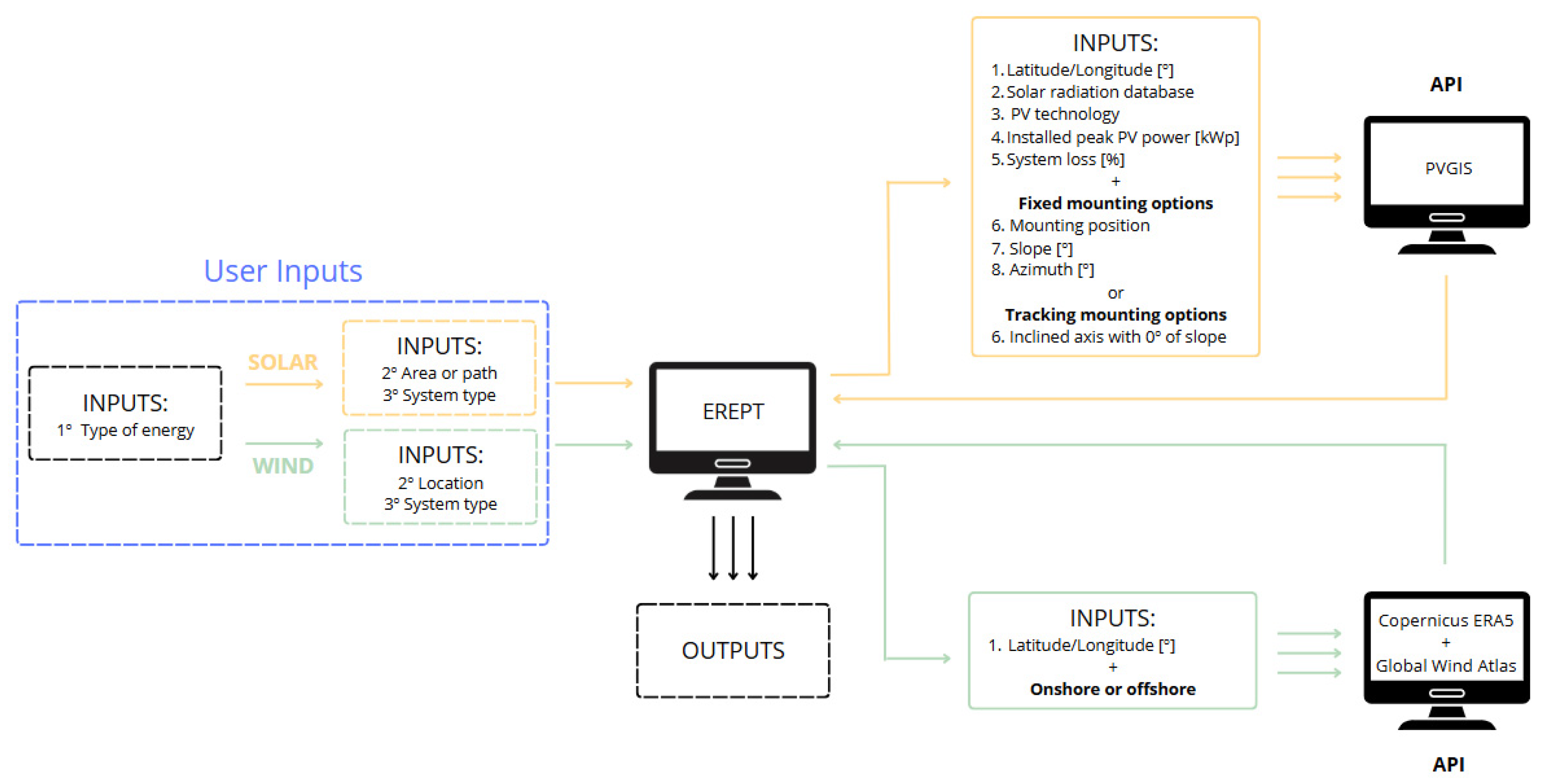
This section describes the methodology adopted in the development of this tool, for its different functionalities: simulation of renewable energy (solar and wind) and energy storage systems, economic analysis of these components, and calculation of the carbon footprint (Figure 1).

2.1. Energy Production Simulations

To simulate solar photovoltaic and wind energy production, the tool uses an Application Programming Interface (API) (Figure 1) that acts as an intermediary, allowing for the Bee2CleanEnergy tool to communicate with the PVGIS [27], Copernicus ERA5 [28] and GWA [29].

2.1.1. Solar Photovoltaic

Before the photovoltaic solar simulation methodology was developed, it was validated by comparing the results obtained through PVGIS and PVSyst programs [21,27]. Since no significant differences were observed, the authors adopted the PVGIS API. PVGIS is a free and simplified online tool that allows users to determine the photovoltaic system performance (e.g., monthly and annual energy production) and meteorological data (e.g., Typical Meteorological Year) in almost any location worldwide [27]. To perform the simulations, it is necessary to provide the following inputs to the program: coordinates (latitude [°]; longitude [°]), solar radiation database, photovoltaic (PV) technology, installed peak photovoltaic power [kWp], system losses, plus mounting position, tilt [°] and azimuth [°] of the module for a fixed system, or axis type and tilt [°] for a tracking system (Figure 1).

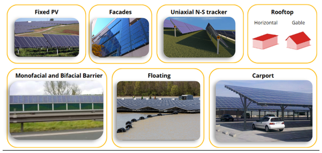
In Bee2CleanEnergy, the coordinates sent to PVGIS correspond to the midpoint of the area or path drawn by the user. Additionally, for any system type, “Crystalline Silicon” will be considered the “PV Technology” parameter, and 14% of system losses by default, as defined in PVGIS. Finally, the solar radiation database to be used must follow the sequence PVGIS-SARAH3 > PVGIS-NSRDB > PVGIS-ERA5, organized from most accurate to least accurate, according to the order of PVGIS and its availability. Despite this transversal approach, addressing the coordinates, PV technology, and system losses, to all systems, a specific approach was considered for each PV typology (Figure 2) that can be simulated: fixed PV, vertical barriers, building integrated (roofs and facades), floating PV, uniaxial N-S tracker, and carports.

It is important to note that to develop the simulation methodology for those PV typologies, it was necessary to consider a typical PV module model. As described throughout the article, the module considered was the EAP500W from Energy America (22.69% efficiency and with dimensions of 2.176 m × 1.096) from the PVSyst library [21]. The main calculation formulas and conditions defined for each PV technology are presented below.

• Fixed PV

In this typology, the “free-standing” mounting position is considered. This type of system is the simplest and most frequently implemented. It is characterized by presenting a fixed azimuth and inclination. These parameters directly impact a module’s energy production; they must be carefully optimized for each specific case. Accordingly, the module’s azimuth was defined to maximize the system’s energy production at the target location. For locations in the northern hemisphere (latitudes ≥ 0°), a southern orientation (azimuth = 0° by PVGIS convention) was assumed, and for locations in the southern hemisphere (latitudes < 0°), an orientation to the north (azimuth = −180° by PVGIS convention) was assumed.

The optimal tilt angle ($\alpha \_opt)$ for maximizing the annual energy production at different locations around the globe was determined by following the work of Jacobson and Jadhav [37]. For the Northern Hemisphere, the optimal tilt angle ($\alpha \_optn)$ is given by Equation (1), whereas for the Southern Hemisphere ($\alpha \_opts)$, it is given by Equation (2), where φ denotes the latitude in degrees.

$$\alpha \_optn \left[°\right]=1.3793+\phi \times \left(1.2011+\phi \times \left(-0.014404+\phi \times 0.000080509\right)\right)$$

(1)

$$\alpha \_opts \left[°\right]=-0.41657+\phi \times \left(1.4216+\phi \times \left(0.024051+\phi \times 0.00021828\right)\right)$$

(2)

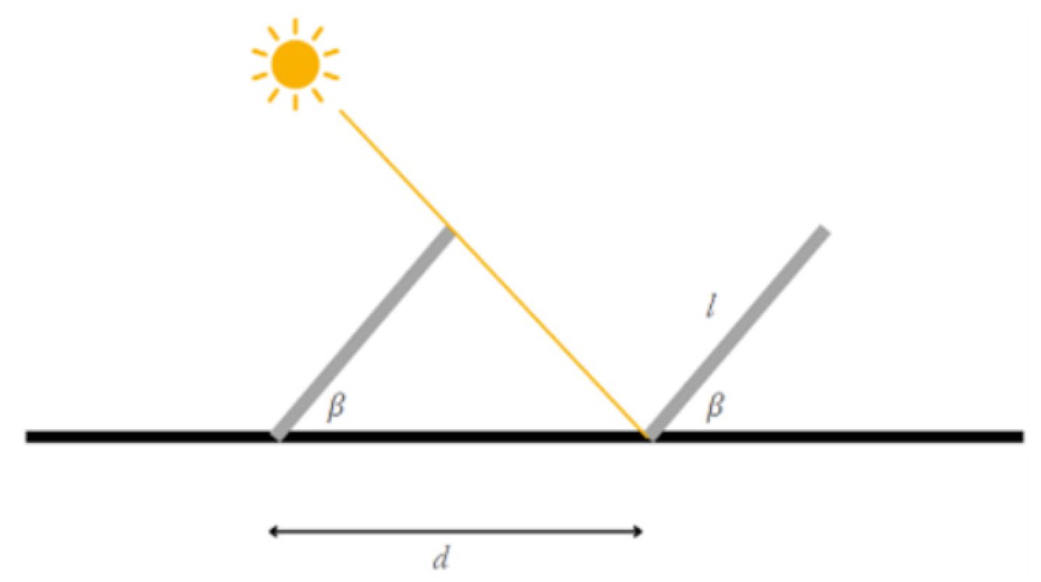
Nevertheless, these equations result in very low slopes for latitudes close to the equatorial line, so for the latitude range of [−10°; 10°], an inclination angle of 10° was considered so that the rain naturally cleans the modules. To determine the installable power per square meter for distinct locations worldwide, the required distance d (Figure 3) was calculated to minimize the shading losses, which depend on the optimal tilt angle.

The parameter d was calculated for the latitudes in the range of [−54°; 66°], in steps of 1°, and is given by expression 3, where l is the length of the module in m (2.176 m), β is the module tilt in degrees, and γ is the solar elevation angle, also in degrees.

$$d=l\times \left[{\displaystyle \frac{\mathrm{s}\mathrm{i}\mathrm{n}\left(\beta \right)}{\mathrm{t}\mathrm{a}\mathrm{n}\left(\gamma \right)}}+\mathrm{c}\mathrm{o}\mathrm{s}(\beta )\right]$$

(3)

The parameter γ is given by expression 4, where h is the hourly solar angle (30°) and δ is the declination in degrees, which is calculated using Formula (5), where N is the day of the year with the fewest hours of sunlight in each location—21 December (n = 355) for the northern hemisphere and 21 June (n = 172) for the southern hemisphere.

$$\gamma =se{n}^{-1}\left[sin\left(\phi \right)\times sin\left(\delta \right)+\cos \left(\phi \right)\times \cos \left(\delta \right)\times \cos \left(h\right)\right]$$

(4)

$$\delta =23.45\times sin\left[{\displaystyle \frac{360}{365}}\times \left(284+n\right)\right]$$

(5)

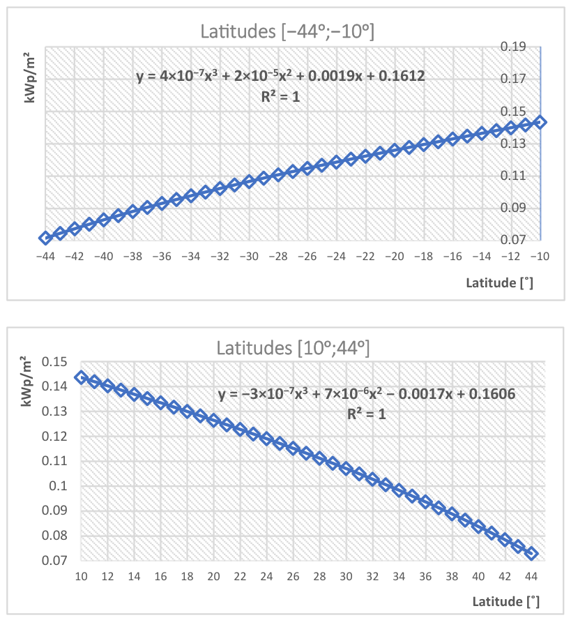
However, next to the south pole and north pole, there is an extreme case—six months of continuous light and six months of darkness. In this way, the calculation of the distance between rows, d, for latitudes > 44° and <−44°, was made for the equinox (corresponding to the beginning of the worst-case scenario: the beginning of six months of darkness), where the declination is 0°. If this calculation were made for the 21st of December or June 21, depending on the location, it would result in higher distances between panels and, consequently, in an excessively large, occupied area that would not be significant, since winter days in these latitudes have few hours of sunlight, which means less solar energy production. Figure 4 shows the linear regression of the results obtained for latitude ranges of −44° to −10° and 10° to 44°.

The equations obtained are represented in

Table 2. Calculation of installed peak power capacity for different latitudes.

Latitudes	Installed Peak Power [kWp]
[−54°; −44°]	(−2 × 10−5 × L2 − 0.0006L + 0.1382) × A 1
[−44°; −10°]	(4 × 10−7 × L3 + 2 × 10−5 × L2 + 0.0019L + 0.1612) × A 1
[−10°; 0°]	(−6 × 10−6 × L2 + 0.0003L + 0.1504) × A 1
[0°; 10°]	(−6 × 10−6 × L2 − 0.0003L + 0.1504) × A 1
[10°; 44°]	(−3 × 10−7 × L3 + 7 × 10−6 × L2 − 0.0017L + 0.1606) × A 1
[44°; 66°]	(−2 × 10−5 × L2 + 0.0005L + 0.1389) × A 1

¹ Useful area.

, where L is the latitude in degrees (°), and the parameter “useful area” (A) corresponds to 90% of the area, in square m (m²), drawn by the user, since there is a portion that will not be used for the installation of PV systems but for other purposes (e.g., access).

• Floating

The floating systems, designed to be installed in water reservoirs such as dams, were modeled based on [38]. Favoring assembly in an east–west delta, the company proposes an inclination of 5° for the equatorial region (latitudes [−6°; 6°]) and 12° for the remaining regions of the globe.

For each project (area designed by the user), the tool will consider the free-standing mounting position and will have to perform two simulations: one for the installed power that is oriented to the west and another for the installed power that is oriented to the east. For each simulation, the tool will consider the installed power (Equation (6)) for the desired orientation, according to the size of the area selected by the user.

Installed peak power [kWp] = 0.18 × 0.5 × A

(6)

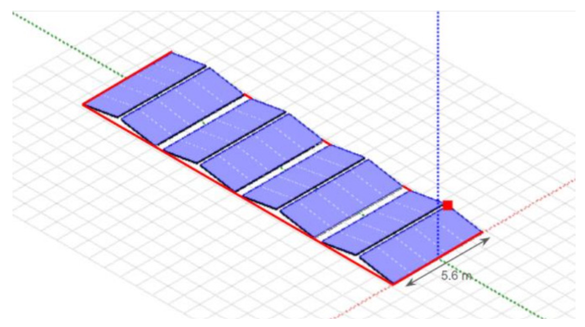
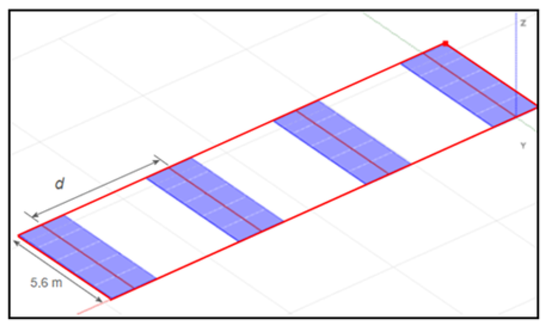
The A parameter is 90% of the area selected by the user, and the value 0.18 [kWp/m²] was determined through a sketch of a 20 kWp system, created in the PVSyst program (Figure 5). Using the program’s measurement tool, it was possible to estimate a width of 5.6 m and a length of approximately 19.6 m for the systems with 5° inclination, and a length of 19.56 m for the system with 12°, regarding the occupied area. These systems have a similar occupied area (area highlighted in red in Figure 5): 0.18 kWp/m² given by the calculation (20 kWp)/(19.6 m × 5.6 m).

The system considers a distance of 0.4 m between rows, ensuring easy access and minimizing the shading between them. Furthermore, it is worth mentioning that the arrangement, in portrait or landscape, of the modules in this type of system can be configured in a way that favors the module characteristics (e.g., number of bypass diodes or half-cell/full-cell modules).

• Vertical Barrier

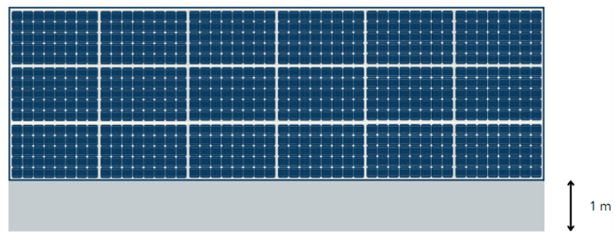
Here, the authors intend to introduce the simulation of photovoltaic systems as a vertical barrier along roads and railways. The configuration of this system is illustrated in Figure 6, where a vertical structure is designed in which the first meter from the ground will be empty or used as a base for the PV system, followed by three modules arranged horizontally in height, as stated in the study [33].

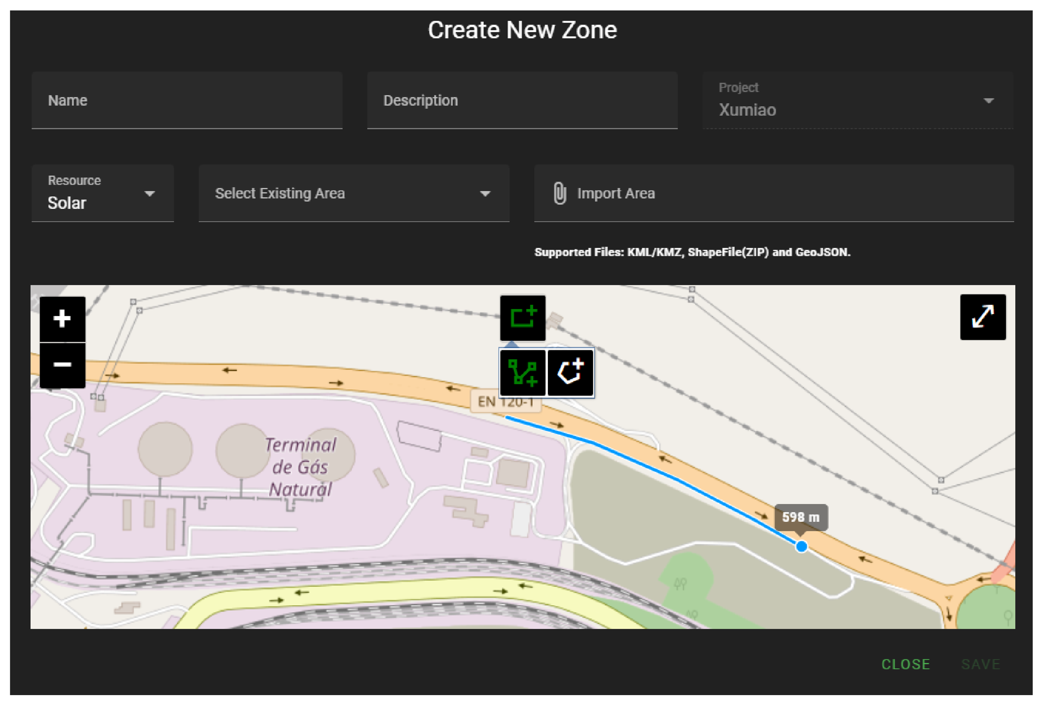
Considering the dimensions of the Energia America EAP500W module, this barrier has a capacity of 0.68 kWp/m. The path drawn by the user can contain several subsegments—a maximum of 500 m each—followed by each other and with different orientations (Figure 7). The tool uses the PVGIS free-standing mode for the system mounting position and calculates (Equation (7)) to determine the power that can be installed in each subsegment.

Installed peak power [kWp] = 0.68 × Segment length

(7)

For each path subsection, the coordinates of its midpoint are used as the latitude and longitude values to be assumed in the simulation. The different azimuths assumed by the tool favor orientation towards the equatorial line. In the case of the bifacial system, the tool will have to request the PVGIS API to perform two simulations, one for each orientation (opposite each other) of each subsegment drawn. It should be noted that, in some cases, east–west oriented bifacial systems may provide greater technical and economic benefits compared to systems with other orientations, as electricity is more expensive at the beginning and end of the day.

• Carport

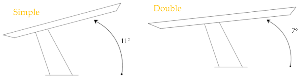
The modeling of this typology was based on the structures of Iziwalker [39] (Figure 8). For the slope of the roof, a value of 9° is assumed, as the average between the slope of a double structure (7°) and the simple structure (11°), making the tool simpler, since the user will not have to specify whether the designed cover is a single or double structure. Furthermore, the error associated with this difference of 2° to 3° in the inclination of the structures is small and not significant.

By default, Bee2CleanEnergy [20] assumes the free-standing mounting position, while the user must provide the roof azimuth. Consistent with the aforementioned photovoltaic typologies, when the perimeter of the parking cover is drawn, only the central coordinates of the area are used to locate the system. The potential of this type of installation is given by the following expression 8.

Installed peak power [kWp] = 0.18 × Parking area

(8)

The 0.18 kWp/m² factor resulted from the analysis of the potential of this type of covering in parking lots in the Port of Sines Authority (APS) jurisdiction area. Through several preliminary 2D sketches drawn in AutoCAD 2025 [40], the average capacity of a parking garage was determined (0.18 kWp/m²) and integrated into expression 8.

• Rooftops

The Bee2CleanEnergy [20] tool integrates the two most common roof types: flat and gable roofs. For gable roofs, the modules are completely embedded in the roof, with little or no air movement behind the system, so the mounting position considered is “roof added/building integrated”. For flat roofs, especially in latitudes that favor low module slopes, there is also little or no air circulation behind the PV system. Therefore, the same mounting position will be adopted.

Regarding the simulation of systems on flat (horizontal) roofs, the tool will use the same method as in the fixed system. However, the equations used to determine the power that is possible to install in the selected roof area follow those presented in Table 2. In this case, the “useful area” parameter is assumed to be 52% [33] of the selected area, instead of 90%, to account for areas where PV installations are not feasible (e.g., areas with obstacles such as chimneys or access paths).

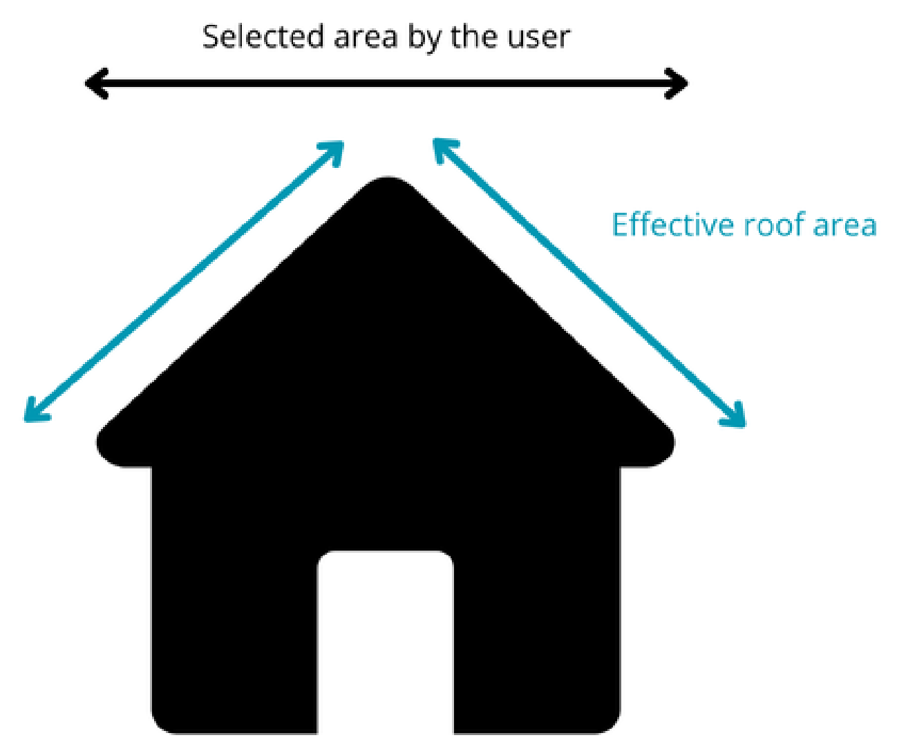
For gable roofs, the authors consider the roof structure illustrated in Figure 9. The user must provide additional information to the tool, namely the roof slope (s) and the orientation of one of the roof surfaces, which are then used in the simulation to configure the photovoltaic system.

Bee2CleanEnergy [20] queries the PVGIS API to run two simulations, one for each roof surface (opposite orientations), and only 52% of the user-selected area (b) is considered for PV installation. It should be noted that the area selected by the user does not correspond to the effective roof surface, as the roof has an oblique slope. This geometric effect justifies the inclusion of the cosine term of the roof slope (cos (s)) in Equation (9), which is used to calculate the installable power on each of the two roof surfaces.

The coefficient 0.21 [kWp/m²] represents the power per square meter of the EAP500 module and results from the calculation (0.500 kWp)/(1.096 m × 2.176 m).

$$\mathrm{Installed} \mathrm{peak} \mathrm{power} [\mathrm{kWp}]=0.52\times (0.5\times b)\times \left[{\displaystyle \frac{0.21}{\mathrm{c}\mathrm{o}\mathrm{s}\left(s\right)}}\right]$$

(9)

• Facades

In this case, the photovoltaic system is placed on the wall of a building. Therefore, the mounting position considered is roof added/building integrated. For the facade simulation, the tool uses Equation (10) to determine the power value to be considered. The Available area (Equation (11)) is given by the length of the facade (h) in m (horizontal dimension), drawn by the user, multiplied by the height of the facade (H) in m (vertical dimension), which is also specified by the user, and multiplied by an estimated percentage of the Available area (effective area [%]) for the integration of photovoltaic modules. In the case of facades without obstacles, the user is advised to conservatively consider a maximum value of 90% for the “effective area” parameter. For the simulation to proceed, the user must also specify the orientation (azimuth).

Installed peak power [kWp] = 0.21 × Available area

(10)

$$\mathrm{Installed} \mathrm{peak} \mathrm{power} [\mathrm{kWp}]=h\times \mathrm{H}\times \left({\displaystyle \frac{effetive area}{100}}\right)$$

(11)

The value 0.21 [kWp/m²] results from the calculation (0.500 [kWp])/(1.096 [m] × 2.176 [m]), where the numerator is the power of the EAP500 module, and the denominator is its dimensions.

• Uniaxial North–South (N–S) Tracker

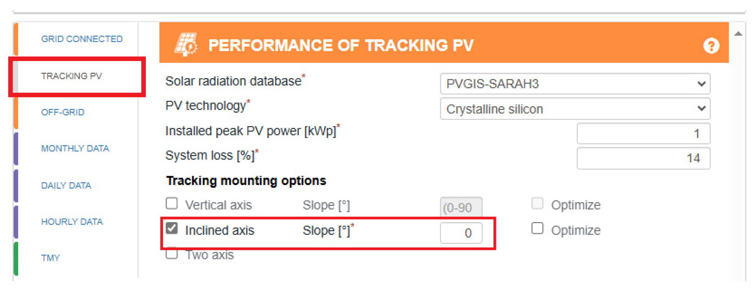
Contrary to the other typologies integrated into the Bee2CleanEnergy tool [20], or a uniaxial tracker with an N-S horizontal axis, the “TRACKING PV” window must be used instead of the “GRID CONNECTED” window of the PVGIS API. Given the nature of this system, a value of 0° is considered for the “inclined axis” parameter (Figure 10). In the PVGIS interface, the asterisk next to the “Inclined axis (slope)” field indicates that this parameter is required by the tool.

Optimizing this type of system involves determining the ideal distance between rows (d), as this influences energy production (Figure 11).

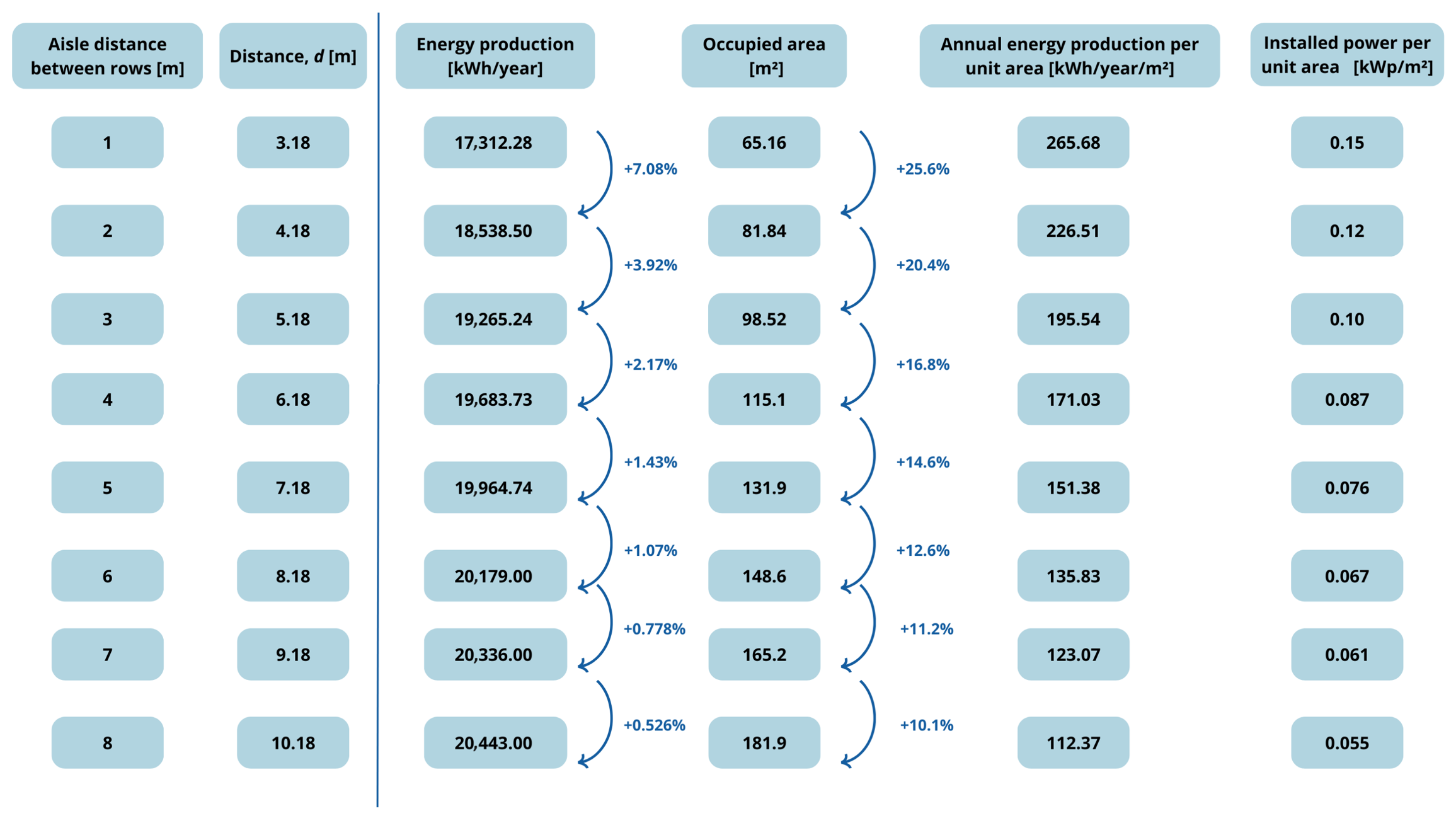
Figure 12 shows the results obtained with PVSyst for the annual energy production and occupied area for different values of d, for a N-S uniaxial solar tracking photovoltaic system with a maximum and minimum inclination θ of +/− 60° (predefined value by PVSyst), equipped with backtracking.

A correlation between annual energy production and the area occupied can be observed: the greater the energy production, the larger the occupied area. Here, percentage increases of up to 7.08% were recorded for a one-meter increase in the value of d. It remains to be determined to what extent the percentage increase in annual production is significant, relative to the corresponding increase in the occupied area. The following graph is important for this assessment.

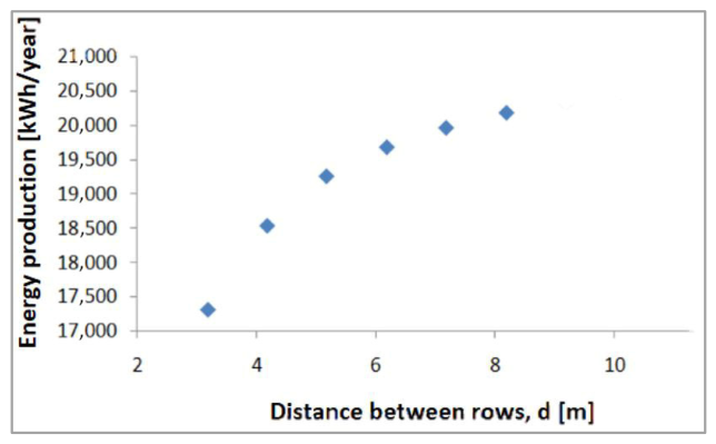
The graph (Figure 13) shows that from 8.18 m of distance between rows, the increase in energy production begins to decrease and stabilize to a limited value. Therefore, for the Tracker typology, row spacing of 8.18 m and a factor of 0.067 kWp/m² will be assumed (Equation (12)). In this case, since there was significant growth in production with the increase in area to be occupied, the annual energy production per unit area was not the determining factor for the selection of distance (d). While maximizing land use is important, maximizing the annual energy production at full system utilization allows for better economic indicators. Accordingly, the installed power is given by the following equation, where the “useful area” is again 90% of the area selected by the user.

Installed peak power [kWp] = 0.067 × A

(12)

2.1.2. Wind

The wind simulations were based on the hourly data provided by Copernicus ERA5 [27] and GWA [29], via the API service. The ERA5 is a climate and weather reanalysis dataset from 1940 to the present. It is part of the Copernicus Climate Change Service and is produced by the European Center for Medium-Range Weather Forecasts. ERA5 provides hourly estimates of atmospheric, oceanic, and land surface variables [24].

The GWA [29] is a free, web-based platform that provides online wind resource information, including wind speed and direction, among other parameters, enabling users to identify high-wind areas that are suitable for wind power generation. The GWA version 3.3 was developed [29], owned, and operated by the Technical University of Denmark (DTU). This latest version was released in partnership with the World Bank Group, utilizing data provided by Vortex and funded by the Energy Sector Management Assistance Program (ESMAP) [20].

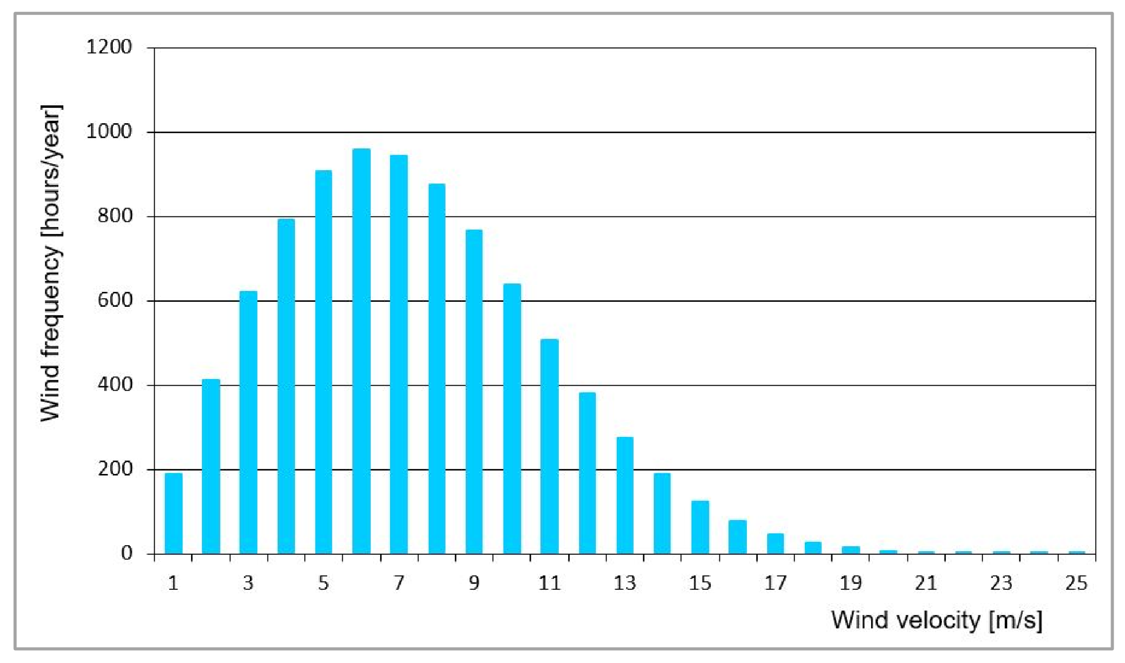
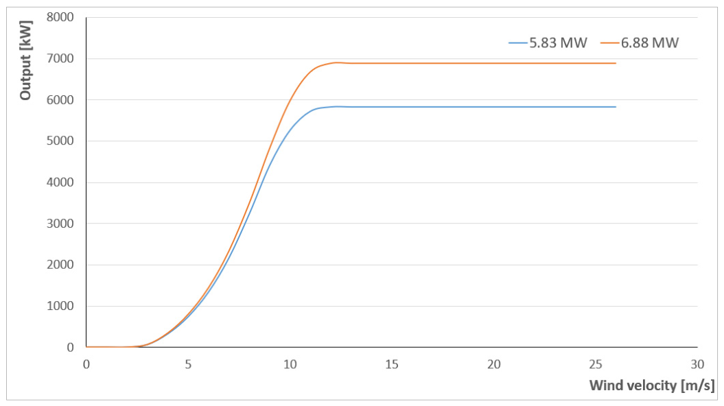
For the calculation model, Bee2CleanEnergy [20] considers two generic turbine models: one with a peak power of 5.83 MW and another with a peak power of 6.88 MW. In general, Bee2CleanEnergy [20] sends the coordinates of the simulation point to the GWA [29], which returns the local Weibull scale factor (a in m/s), representing the characteristic wind speed of the distribution and the Weibull (Figure 14) shape factor (k) at 100 m altitude. With values of a and k, it is possible to calculate the wind speed availability (expression 13) [41].

$$\mathrm{Wind} \mathrm{availability} \left[{\displaystyle \frac{\mathrm{h}\mathrm{o}\mathrm{u}\mathrm{r}}{\mathrm{y}\mathrm{e}\mathrm{a}\mathrm{r}}}\right] =\left[{\displaystyle \frac{k}{a}}\times {\left({\displaystyle \frac{v}{a}}\right)}^{k-1}\times \exp \left(-{\left({\displaystyle \frac{v}{a}}\right)}^k\right)\right]\times 365\times 24$$

(13)

The figure below shows an example of the Weibull probability density function (k = 2.18; a = 8.3 m/s) [41].

Thus, wind production is obtained by multiplying the number of hours at each average wind speed [hours/year] by the power output of the wind turbine at each wind velocity [kW], as shown in Equation (14).

$$\mathrm{Wind} \mathrm{energy} \mathrm{production} \left[{\displaystyle \frac{\mathrm{k}\mathrm{W}\mathrm{h}}{\mathrm{y}\mathrm{e}\mathrm{a}\mathrm{r}}}\right]=\sum \mathrm{Wind} \mathrm{frequency}\times \mathrm{Power} \mathrm{output}$$

(14)

Figure 15 shows the power curves of the two turbines used as the basis for the wind simulation at an air density of 1.225 [kg/m³].

Moreover, in order to extend the representativeness of the wind regime characterization, Bee2CleanEnergy [20] extracts the last 20 years of horizontal wind speed (u-component) data. Then, by applying Equation (14) again, it calculates the new wind energy production. Subsequently, linear correlations between the first and second energy production values are used to derive a scaling factor, which can then be applied to the wind regime characterization.

2.2. Storage

Within the context of the Nexus project, an investigation into the integration of energy storage systems, specifically battery energy storage units, into the Bee2CleanEnergy [20] simulation tool was conducted by Batteries and Secure. Currently, the tool allows for simulations of electrochemical energy storage technologies to optimize self-consumption from renewable energy sources, namely solar photovoltaic and wind. This functionality enables the user to estimate the potential energy capacity of containerized batteries, ranging from kWh to MWh scales, based on the available installation area. For this purpose, three different battery storage technologies are considered: lithium-ion, vanadium redox flow, and sodium–sulfur. The selection of these battery technologies was based on their current and projected applicability in medium- to large-scale systems [42,43,44].

Table 3. Parameters of the different electrochemical energy storage technologies considered in the Bee2CleanEnergy [20,45,46,47,48].

Parameter	Vanadium Redox Flow	Lithium-Ion	Sodium–Sulfur
Battery efficiency (charge/discharge) [%]	80	90	90
Power electronics efficiency [%]	95	96	95
Depth of discharge [%]	100	80	100
Lifetime [years]	20	15	20
Degradation in energy capacity [%/year]	0	2	1.8

presents the most relevant parameters of each battery technology considered in this study.

The useful energy capacity of each battery is calculated by taking into account the efficiencies of both the battery and the power electronics, the depth of discharge, and the annual energy capacity degradation. The authors consulted various current manufacturers of these technologies (for 2024) to relate the container size of each technology to its corresponding energy capacity. Two main container sizes were investigated: the 6.1 m and 12.2 m sizes. The following presents the average values of these sizes:

• Lithium-ion: 40 m²/MWh (minimum area: 1 MWh = 40 m²) [49,50,51,52,53,54,55,56,57,58,59,60].
• Vanadium redox flow: 90 m²/MWh (minimum area: 0.4 MWh = 36 m²) [61,62,63].
• Sodium–sulfur: 19 m²/MWh (minimum area: 2.9 MWh = 54 m²) [64,65].

The obtained values present some variability among the same technology, given the different configurations that the distinct manufacturers present and the market/applications that the battery energy storage serves. The approach is a rough estimation, given the dependency on various influence parameters such as geography, existing controls, and refrigeration applications, among others, that deeply affect the battery energy capacity and performance within the containerized solution.

According to the existing standards, the estimated values include both the battery system and the remaining components, such as the Power Conversion System (PCS); controls; and heating, ventilation, and air conditioning (HVAC). In addition to these parameters, lithium-ion battery containers require a minimum separation distance of 3 m from any surrounding object, including other containers. This requirement is based on the National Fire Protection Association (NFPA) standard, which recommends a 3 m separation between outdoor battery containers to prevent exposure to public access routes, buildings, combustible storage materials, hazardous materials, and other non-electrical hazards [66]. When the batteries have the UL 9450 certification, the minimum separation distance can be reduced to 1 m. However, in this study, a conservative approach was adopted. In the case of vanadium redox flow batteries and sodium–sulfur batteries, container stacking is permitted and was therefore considered (with two containers stacked), given their non-explosive electrochemical nature.

2.3. Economic Analysis

In addition to technical assessments, the Bee2CleanEnergy tool [20] can perform economic estimations, allowing users to determine the project’s feasibility. The approach adopted here consists of a preliminary economic assessment, focusing on the key economic indicators of the project for which data are available.

The use of fixed financial coefficients—such as standardized Capital Expenditure/Operating Expenditure (CAPEX/OPEX) benchmarks and working capital percentages—is necessitated by the tool’s function as an early-stage e-DSS. In contexts where the project stage precedes the deployment of dedicated on-site infrastructure [67], these industry benchmarks provide a consistent baseline for comparing technological configurations without the noise of unvalidated stochastic variables. This approach adheres to the principle of framework parsimony [24], ensuring transparency and reproducibility for stakeholders during preliminary screening.

While absolute indicators like the Net Present Value (NPV) or Levelized Cost of Energy (LCOE) may fluctuate with market volatility, the relative ranking of design alternatives remains robust, which is the primary objective of sustainable component-level prioritization [23] in preliminary engineering. By focusing on validated industry coefficients, Bee2CleanEnergy [20] delivers a reliable first-order economic assessment, serving as a strategic precursor to the high-fidelity financial modeling required in subsequent execution phases.

2.3.1. Cash Flow (CF)

CF is the movement of money in a given period, and it can be related to a project or a business. Most simply, the CF is the difference between cash inflows and cash outflows (Equation (15)) [68].

CF [$] = CI − CO

(15)

where the CI is the cash inflow, and CO is the cash outflow, in $.

The total income (In) is the value generated by the energy production, expressed as follows:

In [$] = Produced electricity × c + CWC

(16)

The produced energy is the annual amount of electricity produced by the system [kwh], c is the energy cost [$/kWh], and the CWC is the change in working capital [$] in the t year. This last parameter measures the variation in working capital, which can be expressed as follows:

CWC_(t) [$] = Total investment in working capital _(t−1) − Total investment in working capital _(t)

(17)

where the total investment in working capital is given by the following:

Total investment in working capital [$] = CD + S − DS

(18)

The CD (Equation (19)) is customer debts, the S (Equation (20)) is stock funds, and the DS is debts to suppliers (Equation (21)):

CD [$] = 0.15 × Produced electricity × c

(19)

S [$] = 0.10 × Produced electricity × c

(20)

DS [$] = 0.20 × Produced electricity × c

(21)

In cases where the project receives a subsidy, it is considered an additional income. Conversely, if the project is financed through a bank loan, this corresponds to a cash inflow in the first year, followed by cash outflows in subsequent years during the loan period, including interest payments. Hence, the cash outflow (Out) can be expressed as follows:

Out [$] = CAPEX + OPEX + Land rent (if applicable) + Interest + Loan payment

(22)

The values assumed for CAPEX and OPEX per unit peak power ($/kWp) installed come from the International Renewable Energy Agency (IRENA) [69] and are presented in

Table 4. Solar and wind: CAPEX and OPEX costs assumed in Bee2CleanEnergy [20] as default. Adapted from [69].

Resource	Region	CAPEX $\left[\frac{\mathbf{\$}}{\mathbf{k}\mathbf{W}\mathbf{p}}\right]$	OPEX $\left[\frac{\mathbf{\$}}{\mathbf{k}\mathbf{W}\mathbf{p}.\mathbf{y}\mathbf{e}\mathbf{a}\mathbf{r}}\right]$
Solar	Asia	758	3.6
	Eurasia *		6.6
	Europe		8.4
	North America		9.1
	Oceania		7.7
	South America		7.6
Wind	Onshore	1160	41
	Offshore	2800	79

* Refers to Armenia, Azerbaijan, Georgia, the Russian Federation, and Türkiye.

.

Moreover,

Table 5. The storage system costs were assumed as the default values in Bee2CleanEnergy [20].

System Technologies	CAPEX $\left[\frac{\mathbf{\$}}{\mathbf{k}\mathbf{W}\mathbf{p}}\right]$	OPEX $\left[\frac{\mathbf{\$}}{\mathbf{k}\mathbf{W}\mathbf{p}.\mathbf{y}\mathbf{e}\mathbf{a}\mathbf{r}}\right]$	Decommissioning $\left[\frac{\mathbf{\$}}{\mathbf{k}\mathbf{W}\mathbf{p}}\right]$	Source
Vanadium redox flow	781.2	5.2	-	[38,39]
Lithium-ion	484.8	3.0	2.5	[38,40]
Sodium–sulfur	421.0	9.3	-	[38,41]

shows the costs of implementing a storage system in the projects.

2.3.2. Net Present Value (NPV)

NPV reflects the difference between the present value of benefits and the present value of costs over time. Then, NPV is the economic benefit of the system, which is expressed as follows [70]:

$$\mathrm{NPV} [\$]={\sum }_{t=0}^N{\displaystyle \frac{CF}{{\left(1+i\right)}^t}}$$

(23)

where N is the power plant lifetime, including the construction period, and i is the discount rate.

2.3.3. Dynamic Payback Period

The dynamic payback period of a power plant represents the time required to recover the investment cost while accounting for variable annual cash flows [68]:

$${\sum }_{t=0}^N{\displaystyle \frac{{CF}_t}{{\left(1+i\right)}^t}}=0$$

(24)

where CF_t is the annual cash flow at year t and i is the discount rate.

2.3.4. Internal Rate of Return (IRR)

The IRR is a financial metric to assess the economic viability of a project, and it is expressed as follows [68]:

$${\sum }_{t=0}^N{\displaystyle \frac{{CF}_t}{{\left(1+\mathrm{I}\mathrm{R}\mathrm{R}\right)}^t}}=0$$

(25)

2.3.5. Levelized Cost of Energy (LCOE)

LCOE represents the per-unit cost of electricity, providing a way to compare the cost of electricity from different energy sources, and is expressed as follows [68]:

$$\mathrm{LCOE} = {\displaystyle \frac{{\sum }_{t=0}^N\mathrm{T}\mathrm{o}\mathrm{t}\mathrm{a}\mathrm{l} \mathrm{e}\mathrm{x}\mathrm{p}\mathrm{e}\mathrm{n}\mathrm{d}\mathrm{i}\mathrm{t}\mathrm{u}\mathrm{r}\mathrm{e}}{{\sum }_{t=0}^N\mathrm{T}\mathrm{o}\mathrm{t}\mathrm{a}\mathrm{l} \mathrm{e}\mathrm{n}\mathrm{e}\mathrm{r}\mathrm{g}\mathrm{y} \mathrm{p}\mathrm{r}\mathrm{o}\mathrm{d}\mathrm{u}\mathrm{c}\mathrm{e}\mathrm{d}}}$$

(26)

where the total expenditure is related to the CAPEX of a project, operating and maintenance cost, and taxes and interest costs, all discounted to the present value. The total energy produced is also discounted to the present value.

2.4. Carbon Footprint

Since the Bee2CleanEnergy [20] was developed under the Nexus Agenda, the Port of Sines is the main stakeholder for which detailed and reliable emissions data are available. Although the tool has so far been presented in a general manner and, from a conceptual perspective, can be applied to any port or location, its practical implementation was developed and adapted to the Port of Sines, reflecting the available data and the operational context of this port. The emissions calculation is based on a generic formula that can be applied to different contexts. However, the emission factors used are specific to the Port of Sines. This means that the direct application of the tool to other locations would require the adaptation of these factors to each user’s desire. For this reason, this chapter deliberately focuses on the Port of Sines, while clarifying that extending the tool to other ports would require the use of appropriate local data and emission factors.

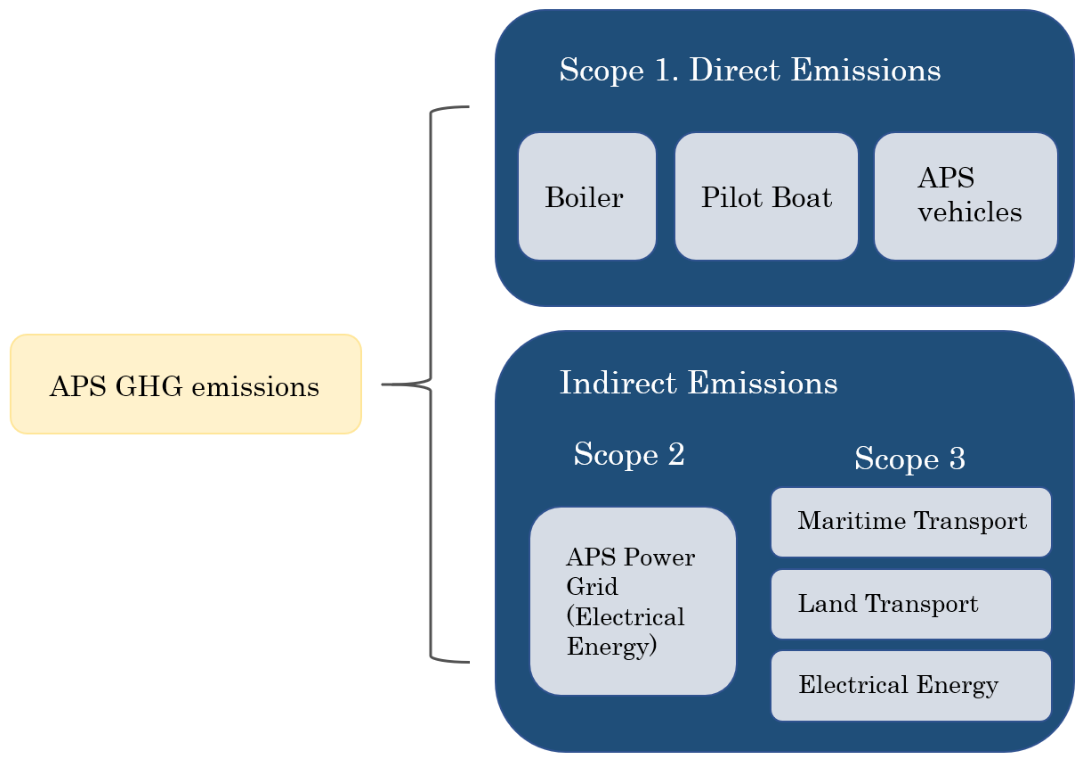
In maritime ports, carbon footprint is associated with the management activities carried out by the port authorities and the operation of terminals, which are generally under concession. The carbon footprint can be estimated using several methodologies, including the GHG Protocol [17], which recommends calculations based on three scopes (as shown in Figure 16). Accordingly, the carbon footprint of the Port of Sines has been calculated using this methodology, based on the data and statistics for the consumption of fixed and mobile facilities (land- and sea-based) within the port’s area of jurisdiction. The practical gaps and implementation challenges of port carbon footprint assessments have been further addressed through sensitivity analysis and scenario-based approaches [71].

For the Bee2CleanEnergy [20] carbon footprint simulation, data and statistics on the consumption of fixed and mobile facilities (land- and sea-based) within the port’s area of jurisdiction was used, as described below:

• Scope 1. Direct emissions of GHG depend on the Port Authority. These emissions include fuel consumption for the transport of ship pilots (pilot boats), land transportation of employees, emergency power plants, and gas use for boilers. To calculate the carbon footprint of this scope, Sines’ Port Authority’s (APS, in Portuguese) data on fuel type and consumption and their respective emission factors are used.
• Scope 2. Indirect emissions related to the generation of electricity acquired and consumed by the Port. This Scope uses the record of energy consumption kept by APS at its facilities and the Portuguese Environment Agency (APA, in Portuguese) [72] emissions factor for each year of the study.
• Scope 3. Other indirect emissions are dependent on concessionaires. The Port of Sines has five specialized terminals (liquid bulk, liquefied natural gas, petrochemical, containers, and general cargo) and includes a marina and fishing ports. To calculate their contribution to the carbon footprint, the emissions due to the operation of each terminal were classified by their consumption of electric energy (acquired through APS and other companies) and maritime and land transport, according to its movements in the port’s jurisdiction area.

In the present calculation tool, average emission factors are estimated based on the cargo handled by each terminal over the period 2018–2022. This emission factor is obtained for each terminal, allowing the carbon footprint to be calculated in a general manner by using the following equation:

Terminal emission [tCO_2eq] = Terminal emission factor × Cargo

(27)

The terminal emission factor is expressed as the equivalent amount of carbon dioxide per amount of cargo, in tons [t], or the number of vessel types attending to each terminal [tCO_2eq/t or tCO_2eq/vessel].

The mitigation of Scope 2 emissions within the Bee2CleanEnergy [20] framework is operationalized through a dynamic displacement algorithm that synchronizes local hourly renewable generation with the time-varying emission intensity of the National Grid. By prioritizing ‘behind-the-meter’ consumption of wind and solar energy, the model calculates the instantaneous avoidance of grid-supplied electricity, directly reducing the carbon footprint associated with purchased energy. As highlighted in the recent literature on Sustainable Design Engineering [73], this methodology advances beyond static annual averages by integrating dynamic indicators into design scenarios, thus providing a high-resolution assessment of the carbon neutrality potential. This approach ensures that the energy–storage–carbon nexus serves as a primary design constraint, facilitating a rigorous evaluation of decarbonization targets during the preliminary planning phase.

3. Case Study: Port of Sines

The Bee2CleanEnergy [20] framework is strategically conceptualized as a deterministic screening tool tailored for the front-end engineering design (FEED) phase, where prioritizing framework usability is essential to establish a robust baseline for technical feasibility. As emphasized in recent studies regarding user-friendly Decision Support Systems [74,75], minimizing excessive model dimensionality during the preliminary stages ensures that the core design logic remains accessible and transparent for stakeholders. By maintaining a reproducible and transparent [23] workflow, the tool facilitates a direct benchmarking process against industry-standard simulation methodologies, which typically rely on fixed-point inputs for early-stage feasibility reporting. This approach is particularly vital in contexts where the project stage precedes the deployment of dedicated on-site infrastructure [67], enabling a reliable first-order approximation that leverages global datasets while avoiding the uncertainty that is inherent in invalidated probabilistic variables.

To test the viability of the Bee2CleanEnergy tool [20], the technical and economic potential of energy production systems through renewable sources, such as solar and wind, and their economic viability were evaluated in the AJP. The carbon footprint and storage simulations were not performed, as these components were still under development at the time of this study.

3.1. Solar Photovoltaic Energy

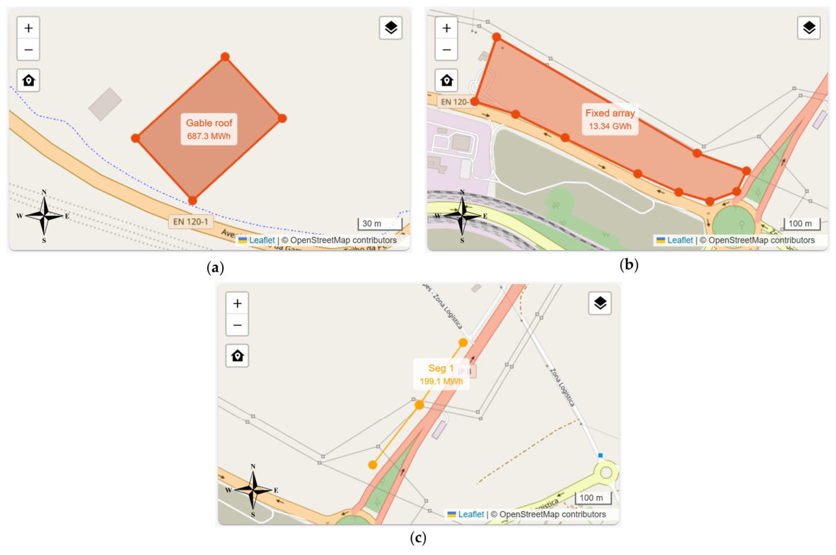
Figure 17 highlights several locations within the AJP that were simulated using the tool to assess their PV potential. These locations include:

• System integration on a gable roof.
• Fixed array on open land.
• Bifacial vertical barrier along roadways.

Table 6. Photovoltaic potential of different areas according to Bee2CleanEnergy [20].

System Typology	Variable	PVSyst	Bee2Clean	Relative Error [%]
McWide (Gable roof)	Installed power [kWp]	460	491.6	4.8
	Energy production [MWh/year]	651	670.2	3.0
Free area (Fixed PV)	Installed power [kWp]	3846	3610	6.1
	Energy production [MWh/year]	6118	6980	14.1
Vertical PV barrier (bifacial)	Installed power [kWp]	295	288.3	2.3
	Energy production [MWh/year]	476,827	414,000	13.2

presents the results obtained for the PV potential of the studied locations, using both PVSyst and the developed tool, with similar simulation parameters applied.

In general, the values obtained from Bee2CleanEnergy [20] closely match those from PVSyst, suggesting that the tool provides reliable estimates of PV energy production for the simulated configurations. The highest relative errors were observed for the fixed array (14%) and the vertical barrier (13%). This discrepancy is likely due to terrain orography, which is not accounted for in the tool, highlighting a limitation that may be significant for sites with complex topography. These findings are consistent with previous studies, which report that PV simulation tools can exhibit differences of up to 10% compared to the actual measured values [67]. Moreover, differences between the existing tools are also observed, with some being more accurate than others, depending on the specific PV system being simulated [68].

Despite the deviations, the projected payback period of approximately 8 years, a NPV of 5.3 million $, and a levelized cost of energy of 48 $/MWh indicate that all three configurations remain economically viable, reinforcing the practical usefulness of the tool in preliminary project assessments.

3.2. Wind Energy

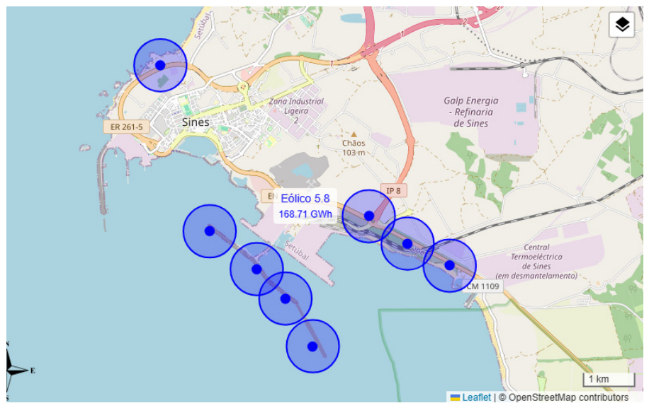
For the wind energy estimation, eight wind turbine positions were established within the AJS. Figure 18 illustrates the location of each turbine.

Similar to the validation performed for the solar results, the Bee2CleanEnergy wind estimations were compared to a study conducted by INEGI [22], which includes projections using turbines from various manufacturers with capacities ranging from 5.5 MW to 7.2 MW. The production performance results from both Bee2CleanEnergy [20] and the INEGI [22] technical study are detailed in

Table 7. AJS wind farm energy estimation comparison between INEGI [22] and Bee2CleanEnergy [20].

System Technology	Installed Power [MWp]	Energy Production [MWh/year]	Energy Production Relative Error [%]
INEGI Study (average)	50	141,887	-
Model 1 (5.83 MW)	47	168,710	19
Model 1 (6.88 MW)	55	177,240	25

.

Due to the confidentiality of the turbine power curves used in the INEGI study [22], only an average value from the aforementioned study is reported. This may explain the significant differences observed between the technical study and the Bee2Clean models (19% and 25%), as the technical results are aggregated into a single average value. Moreover, the models implemented in the tool are generic models, meaning that they do not correspond to any specific wind turbines that are currently available on the market. Nevertheless, considering the purpose of the tool as an early-stage assessment instrument and the inherent uncertainties associated with aggregated reference data and generic turbine models, the observed deviations are within a reasonable range for a preliminary evaluation of the wind energy potential of a given area, providing users with an initial understanding of the local energy potential.

The estimation of the APS wind farm project has a payback of 7 years, an NPV of approximately 159 million $, and an LCOE of 51.7 $/MWh.

4. Conclusions

This paper presents an overview of the technical features of Bee2CleanEnergy [20]. With this tool, the user can simulate the energy production and performance of solar and wind resources at a requested location. Moreover, the economic and carbon footprint behavior is also provided.

Under the Bee2CleanEnergy simulation [20], the Port of Sines shows promising results. It is clear that wind energy alone can meet all the energy needs of APS. However, from a planning perspective, a phased installation of turbines may be advisable, as the energy demand is expected to increase over time and immediate full-capacity deployment may not be necessary. Nevertheless, PV projects, due to their installation flexibility, can be easily implemented in ports and cities. Moreover, compared to wind power, most PV technology requires less investment, both upfront and in maintenance.

Overall, the comparison of results indicates that Bee2CleanEnergy [20] provides reliable estimates for preliminary renewable energy assessments. While the highest relative errors for solar configurations were observed in fixed arrays (14%) and vertical barriers (13%)—likely due to terrain orography parameters—the Bee2CleanEnergy [20] estimates for wind energy production (19% and 25%) are also scientifically consistent with the requirements of the front-end engineering design phase. These wind energy deviations, which are attributed to the use of aggregated average values and generic model assumptions, are expected in regions characterized by data scarcity. As noted in the recent literature, high-fidelity forecasting is often challenging or even impossible [74] in specialized industrial hubs like the Port of Sines, where the project stage precedes the deployment of dedicated on-site infrastructure [67]. Consequently, the developed workflow addresses the gap in research that often neglects specific areas due to severe data scarcity [67], prioritizing the systemic integration of energy, storage, and carbon indicators to provide a robust foundation for initial investment decisions before extensive field measurement campaigns are conducted.

Integration of this tool into the decision-making process represents a valuable contribution to the energy transition in ports. By enabling an early assessment of local endogenous energy resources, the tool allows for stakeholders to better understand the renewable energy potential of a given area and to evaluate the economic viability of potential projects without resorting to time-consuming and resource-intensive studies. Bee2CleanEnergy [20] provides reliable results for a preliminary assessment, with minimal user effort, as it does not require detailed inputs such as optimal panel tilt and azimuth, as required by tools like PVsyst [21], nor complex data processing procedures such as those required by WAsP.

Finally, wind and solar energy are the fastest-growing renewable technologies available on the market and are the cornerstone to achieving a sustainable electrification of economic activities. To keep up with the fast pace of worldwide installations, sites in proximity to consumers, especially energy-intensive consumers and industrial activities, must be assessed for their correct value in sustainability.

Nevertheless, one of the tool’s limitations is that it does not screen areas with territorial restrictions, such as environmental and patrimonial prohibitions. Given the multiple territorial constraints, the user must have the sensitivity to identify the most suitable area for their projects. Moreover, in addition to the terrain’s topographic limitation, the tool does not have the capacity to recognize the terrain’s inclination. These constraints contribute to the differences between the Bee2Clean [20] results and the technical studies.

As future developments, the integration of energy storage components into Bee2CleanEnergy [20], together with further consolidation of carbon footprint assessments, is expected. Additionally, the inclusion of wave energy potential is envisaged, along with a more detailed assessment of wave energy installation costs, according to substructure type. The consideration of territorial and planning constraints through the integration of geographical layers as model inputs is also anticipated.

While the current deterministic approach provides a solid foundation for the preliminary carbon and energy assessments, it is recognized that market and climatic volatility introduce long-term uncertainties. Future iterations of this research should aim to integrate uncertainty quantification modules, such as Monte Carlo simulations, to evaluate the impact of fluctuating electricity prices and inter-annual meteorological variability. Expanding the framework to include these stochastic layers will enhance its resilience, transitioning from a preliminary screening tool to a high-fidelity system that is capable of supporting advanced investment decisions in later project stages.

References

1. Milosavljević, D.D.; Kanivets, T.S.; Jurić, S.J. Review and validation of photovoltaic solar simulation tools/software based on case study. Open Phys. 2022, 20, 431–451. [Google Scholar] [CrossRef] [Scilit]
2. Islam, M.A.; Amin, M.N.; Bin-I-Bari, B.H.; Saikh, S.J.; Tasnim, F.A.; El-Barmawi, C.Z. A comprehensive evaluation of photovoltaic simulation software: A decision-making approach using Analytic Hierarchy Process and performance analysis. Energy Strategy Rev. 2025, 58, 101663. [Google Scholar] [CrossRef] [Scilit]
3. Yılmaz, U.B.; Fidan, S.L.S. Simulation framework for wind energy attributes with WAsP. Procedia Comput. Sci. 2019, 158, 458–465. [Google Scholar] [CrossRef] [Scilit]
4. Meziane, F.C.; Meziane, M.K.; Noureddine, I.; Khellaf, N. Wind flow simulation and characteristics prediction using WAsP software for energy planning over the region of Hassi R’mel. Int. J. Green Energy 2021, 18, 634–644. [Google Scholar] [CrossRef] [Scilit]
5. Okumus, I.; Dinler, A. Current status of wind energy forecasting and a hybrid method for hourly predictions. Energy Convers. Manag. 2016, 123, 362–371. [Google Scholar] [CrossRef] [Scilit]
6. Zhang, Z.R.; Wang, L.Y.; Yang, Y. Port carbon emission estimation: Principles, practices, and machine learning applications. Transp. Res. Part E Logist. Transp. Rev. 2025, 199, 104159. [Google Scholar] [CrossRef] [Scilit]
7. SeaRates. CO2 Calculator Carbon Emissions Calculator for Freight Shipping. Available online: https://www.searates.com/carbon-emissions-calculator/ (accessed on 17 November 2025).
8. Azarkamand, S.; Faure, G.; Del Rosal, M. Calculating the Carbon Footprint in ports by using a standardized tool. Sci. Total Environ. 2020, 734, 139407. [Google Scholar] [CrossRef] [Scilit]
9. Azarkamand, S. Development of a Standardized Tool to Calculate Carbon Footprint in Ports. Ph.D. Thesis, Universitat Politècnica de Catalunya, Barcelona, Spain, 2021. [Google Scholar]
10. Flikkema, M.W.; Ruijter, P.A.J.F.; Ter van Moon, J.D.M.; Schmidt, M. MAGPIE: Towards the European Green port of the Future. Transp. Res. Procedia 2023, 72, 187–194. [Google Scholar] [CrossRef] [Scilit]
11. MAGPIE. Carbon Emissions in Port Areas: An Interactive Visualisation Tool. Available online: https://www.magpie-ports.eu/carbon-emissions-in-port-areas-an-interactive-visualisation-tool/ (accessed on 17 November 2025).
12. Porto de Aveiro; Universidade de Aveiro. Vehicle CO2 Calculator. Available online: https://portodeaveiro.pt/calculadora-emissoes-carbono/ (accessed on 17 November 2025).
13. Emi-Cast Researchers. Calculator—Emicast. Available online: https://emi-cast.com/calculator/ (accessed on 17 November 2025).
14. European Maritime Safety Agency (EMSA). THETIS-MRV Public Emission Report. Available online: https://mrv.emsa.europa.eu/#public/emission-report (accessed on 17 November 2025).
15. DMSLOG.Ai. AI-Powered Solutions. Comprehensive Tools to Optimize Every Aspect of Container Terminal Operations. Available online: https://dmslog.ai/solutions/#co2-monitor (accessed on 23 March 2026).
16. ABB. CO2e Calculator Marine & Ports. Available online: https://new.abb.com/marine/co2e-calculator (accessed on 17 November 2025).
17. Greenhouse Gas Protocol. GHG Protocol: Standards & Guidance. Available online: https://ghgprotocol.org/standards-guidance (accessed on 27 February 2025).
18. Nguyen, T.A.; Byrne, R.H. Software tools for energy storage valuation and design. Curr. Sustain. Renew. Energy Rep. 2021, 8, 156–163. [Google Scholar] [CrossRef] [Scilit]
19. Enasel, E.; Dumitran, G. Storage solutions for renewable energy: A review. Energy Nexus 2025, 17, 100391. [Google Scholar] [CrossRef] [Scilit]
20. ITGest. Bee2CleanEnergy, v.0.0.38; ITGest: Luanda, Angola, 2026. Available online: https://qual-ai-01.itgest.pt:36024/ (accessed on 30 March 2025).
21. PVSyst SA. PVsyst: Photovoltaic Software, Design and Simulate Photovoltaic Systems. Available online: https://www.pvsyst.com/ (accessed on 26 August 2025).
22. INEGI. Instituto de Ciência e Inovação em Engenharia Mecânica e Engenharia Industrial—Wind Energy. Available online: https://www.inegi.pt/en/how-we-work/services-for-industry/consulting/wind-energy/ (accessed on 7 July 2025).
23. Kaur, S.K.; Rao, S.K. Sustainable component-level prioritization of PV panels, batteries, and converters for solar technologies in hybrid renewable energy systems using objective-weighted MCDM models. Energies 2025, 18, 5410. [Google Scholar] [CrossRef] [Scilit]
24. Evola, G.; Tanteri, M.; Costanzo, V.; Leonardi, M.; Abbate, D.; Margani, G. A Decision Support Tool to Assess the Energy Renovation Performance Through a Timber-Based Solution for Concrete-Framed Buildings. Energies 2025, 18, 2839. [Google Scholar] [CrossRef] [Scilit]
25. Nielsen, C. ESG Reporting and Metrics: From Double Materiality to Key Performance Indicators. Sustainability 2023, 15, 16844. [Google Scholar] [CrossRef] [Scilit]
26. Fu, H.M.; Ali, W.; Jiao, J.; Zhang, Z. Hydrogen energy storage via carbon-based materials: From traditional sorbents to emerging architecture engineering and AI-driven optimization. Energies 2025, 18, 3958. [Google Scholar] [CrossRef] [Scilit]
27. European Commission. Getting Started with PVGIS. Available online: https://joint-research-centre.ec.europa.eu/photovoltaic-geographical-information-system-pvgis/ (accessed on 22 October 2024).
28. Copernicus Climate Change Service (C3S). ERA5 Hourly Data on Single Levels from 1940 to Present. Available online: https://cds.climate.copernicus.eu/ (accessed on 14 March 2026).
29. DTU Wind Energy; World Bank Group. Global Wind Atlas. Available online: https://globalwindatlas.info/ (accessed on 22 October 2024).
30. Addens. Empresas de Montagem de Painel Solar. Available online: https://www.addens.com.br/ (accessed on 31 March 2025).
31. Architecture Masterprize. Solar Facade System/Elemex Architectural Facade Systems. Available online: https://architectureprize.com/winners/winner.php?id=4496 (accessed on 31 March 2025).
32. HD Solar. Single Row Flat Single Axis Tracker. Available online: https://www.hdsolartech.com/ (accessed on 31 March 2025).
33. Kakoulaki, G.; Taylor, N.; Spisto, A.; Jäger-Waldau, A. Communication on the potential of applied PV in the European Union: Rooftops, reservoirs, roads (R3). EPJ Photovolt. 2024, 15, 5. [Google Scholar] [CrossRef] [Scilit]
34. Euronews. Projeto Europeu Aposta em Painéis Solares nas Estradas Para Producir Energia. Available online: https://pt.euronews.com/ (accessed on 31 March 2025).
35. Solarfloat. Floating PV Systems. Available online: https://www.solarfloat.com/ (accessed on 31 March 2025).
36. Hanjin. PV Solar Parking. Available online: https://commons.wikimedia.org/wiki/File:PV_solar_parking.jpg (accessed on 27 February 2026).
37. Jamil, M.Z.; Jadhav, V. World estimates of PV optimal tilt angles and ratios of sunlight incident upon tilted and tracked PV panels relative to horizontal panels. Sol. Energy 2018, 169, 55–66. [Google Scholar] [CrossRef] [Scilit]
38. Ciel; Terre. Hydrelio aiR Optim. Available online: https://ciel-et-terre.net/ (accessed on 31 March 2025).
39. IZIWALKER. Solar Shade—Izishader Series. Available online: https://iziwalker.pt/ (accessed on 31 March 2025).
40. Autodesk. Autodesk Software Solutions for Engineering. Available online: https://www.autodesk.com/ (accessed on 31 March 2025).
41. HOMER Energy. Weibull Distribution in Power Systems. Available online: https://homerenergy.com/ (accessed on 27 February 2026).
42. Poullikkas, A. A comparative overview of large-scale battery systems for electricity storage. Renew. Sustain. Energy Rev. 2013, 27, 778–788. [Google Scholar] [CrossRef] [Scilit]
43. International Energy Agency (IEA). Batteries and Secure Energy Transitions. Available online: https://www.iea.org/reports/batteries-and-secure-energy-transitions (accessed on 3 April 2025).
44. Vaska, M.; Sirovy, M. In Proceedings of the 25th 2020 International Conference on Applied Electronics, Pilsen, Czech Republic, 8–9 September 2020; University of West Bohemia: Pilsen, Czech Republic, 2020; Available online: https://searchworks.stanford.edu/view/13803870 (accessed on 23 March 2026).
45. Dong, Z.; Tao, Y.; Lai, S.; Wang, T.; Zhang, Z. Powering Future Advancements and Applications of Battery Energy Storage Systems Across Different Scales. Energy Storage Appl. 2025, 2, 1. [Google Scholar] [CrossRef] [Scilit]
46. Viswanathan, V.; Kendall, M.R.; Frazer, R.X.; Li, L. 2022 Grid Energy Storage Technology Cost and Performance Assessment. PNNL Rep. 2022, 2022, 1–151. [Google Scholar]
47. National Academy of Sciences. Critical Materials in Large-Scale Battery Applications; National Academy of Sciences: Washington, DC, USA, 2012. [Google Scholar]
48. US Department of Energy (DOE). Technology Strategy Assessment Findings from Storage Innovations 2030 Sodium Batteries. Available online: https://www.energy.gov/oe/storage-innovations-2030 (accessed on 3 April 2025).
49. Contemporary Amperex Technology Co., Limited (CATL). EnerOne—Liquid-Cooled Battery Energy Storage System Technical Specifications; Technical Datasheet; Contemporary Amperex Technology Co. Limited: Ningde, China, 2023. [Google Scholar]
50. Società per Azioni. Utility-Scale Battery Energy Storage System (BESS) Design IEC-4.0 MWh System Design; Technical Report; ABB S.p.A.: Bergamo, Italy, 2024. [Google Scholar]
51. Tesla. Megapack Datasheet. Available online: https://www.tesla.com/megapack (accessed on 27 February 2026).
52. Contemporary Amperex Technology Co., Limited (CATL). Storing Infinite Energy: Product Specifications; Technical Datasheet; Contemporary Amperex Technology Co. Limited: Ningde, China, 2024. [Google Scholar]
53. Jinko Solar. Energy Storage Solutions (ESS). Available online: https://www.jinkosolar.com/en/site/ess (accessed on 3 April 2025).
54. Konka Energy. 20′ Feet BESS Container Air Cooling. Available online: https://konkaenergy.com/ (accessed on 3 April 2025).
55. Evlithium. CATL Containerized Energy Storage System; Technical Specifications; Evlithium: Hong Kong, China, 2023; Available online: https://www.evlithium.com/battery-energy-storage-system.html (accessed on 23 March 2026).
56. Hithium. Hithium Energy Storage Products. Available online: https://en.hithium.com/ (accessed on 3 April 2025).
57. Voltail-Battery. Energy Storage System 20Ft Container. Available online: https://www.voltai-battery.com/ (accessed on 3 April 2025).
58. Bluesun Solar. BESS Container Energy Storage Solution. Available online: https://www.bluesunpv.com/ (accessed on 27 February 2026).
59. EIKTO. 20ft/40ft Container & BESS Commercial. Available online: http://www.eikto.com (accessed on 3 April 2025).
60. GoGreen. Containerized Energy Storage System (CESS). Available online: https://www.oegreenpower.com/ (accessed on 3 April 2025).
61. Invinity Energy Systems. Invinity VS3-022 Six Pack Vanadium Flow Battery. Available online: https://invinity.com/ (accessed on 27 February 2026).
62. Energy Storage Solutions. Vanadium Redox Flow Battery 50 KW (200 KWh). Available online: https://energystoragesolutions.com/ (accessed on 27 February 2026).
63. Sumitomo Electric. Flow Battery: Features and Applications. Available online: https://sumitomoelectric.com/ (accessed on 3 April 2025).
64. NGK Insulators. NAS Batteries Product Specifications. Available online: https://www.ngk-insulators.com/ (accessed on 27 February 2025).
65. NGK Insulators. NAS Batteries Start Commercial Operation at BASF’s Schwarzheide Site. Available online: https://www.ngk-insulators.com/en/news/20240318_1.html (accessed on 4 April 2025).
66. National Fire Chiefs Council. Grid Scale Battery Energy Storage System Planning—Guidance for FRS. Available online: https://www.north-herts.gov.uk/ (accessed on 27 February 2026).
67. Ma, Y.T.; Dong, F.Y.; Yang, A.M.; Gantumur, U.C.; He, C.H.; Wang, N. A Systematic Analysis Method for Energy Systems Characterized by Data Scarcity: A Case Study of Mongolia. Sustainability 2026, 18, 2398. [Google Scholar] [CrossRef] [Scilit]
68. Tian, Y.Z.; Zhang, T.Z.; Zhang, Z.X.; Wang, Z.C.; Rong, X.X. Comprehensive economic analysis of adiabatic compressed air energy storage system based on electricity spot market policy. J. Energy Storage 2024, 90, 114333. [Google Scholar] [CrossRef] [Scilit]
69. IRENA. Renewable Power Generation Costs in 2023. Available online: https://www.irena.org/ (accessed on 27 February 2026).
70. Li, P.L.; Gu, G.L.; Jin, S.H.; Hu, H.X.; Zhang, H.Z. Performance comparison and multi-objective optimization of improved and traditional compressed air energy storage systems integrated with solar collectors. J. Energy Storage 2023, 72, 106149. [Google Scholar] [CrossRef] [Scilit]
71. Issa-Zadeh, S.; Bakhshi, E.M.; Delgado, L.G.; Sanchez, J.S.; Garcia-Ramos, C.L. The practical gaps and implementation challenges of port carbon footprint assessments. J. Mar. Sci. Eng. 2024, 12, 1290. [Google Scholar] [CrossRef] [Scilit]
72. Agência Portuguesa do Ambiente (APA). Fator de Emissão de Gases com Efeito de Estufa da Eletricidade Produzida em Portugal 2024. Available online: https://apambiente.pt/ (accessed on 27 February 2025).
73. Komarzyńska-Świeściak, E.; Świeściak, M.; Al-Ani, A.; Taskinen, A.U. Comparative Assessment of Finnish University Campus Transformation. Sustainability 2025, 17, 10425. [Google Scholar] [CrossRef] [Scilit]
74. Tsoumplekas, G.A.; Christodoulou, D.D.; Iliadis, C.A.; Papageorgiou, M.P. Few-shot load forecasting under data scarcity in smart grids: A meta-learning approach. Energies 2025, 18, 742. [Google Scholar] [CrossRef] [Scilit]
75. Chen, J.D.; Tan, T.L.; Li, M.W.; Wang, H. Multi-objective optimization of a regional water–energy–food system considering environmental constraints: A case study of Inner Mongolia, China. Int. J. Environ. Res. Public Health 2020, 17, 6758. [Google Scholar] [CrossRef] [Scilit]
Figure 1. Diagram of the Bee2CleanEnergy API [20] functions for simulating renewable energy systems.
Designs 10 00048 g001
Figure 2. Types of photovoltaic systems included in Bee2CleanEnergy: fixed PV [30], facades [31], Uniaxial N-S tracker [32], rooftop [33], Monofacial and Bifacial Barrier [34], floating [35] and carport [36].
Designs 10 00048 g002
Figure 3. Schematic representation of d, l, and β.
Designs 10 00048 g003
Figure 4. Linear regression of possible installed power per square meter in function of latitudes [−44°; −10° [and] 10°; 44°].
Designs 10 00048 g004
Figure 5. Sketch of a 20 kWp delta system. Source: Adapted from PVSyst [21].
Designs 10 00048 g005
Figure 6. Vertical barrier layout.
Designs 10 00048 g006
Figure 7. Path drawn in the “Create New Zone” window of the Bee2CleanEnergy tool developed by the authors [20].
Designs 10 00048 g007
Figure 8. Conceptual diagram developed by the authors, based on [39].
Designs 10 00048 g008
Figure 9. Representation of the effective roof area.
Designs 10 00048 g009
Figure 10. PVGIS “Performance of tracking PV” window. Source: Adapted from PVGIS [18].
Designs 10 00048 g010
Figure 11. Uniaxial N–S tracker layout. Source: Adapted from PVSyst [21].
Designs 10 00048 g011
Figure 12. Annual energy production by distance, d.
Designs 10 00048 g012
Figure 13. Energy production as a function of the distance between rows.
Designs 10 00048 g013
Figure 14. Weibull probability density function [41].
Designs 10 00048 g014
Figure 15. Bee2CleanEnergy’s wind turbine power curve at an air density of 1.225 kg/m3.
Designs 10 00048 g015
Figure 16. GHG protocol scopes (1, 2 and 3): applications to the APS (author’s work).
Designs 10 00048 g016
Figure 17. Solar simulation of a PV system on a (a) gable roof, a fixed array on open land (b), and (c) a bifacial vertical barrier along a road, using Bee2CleanEnergy [20].
Designs 10 00048 g017
Figure 18. Simulation of a wind farm layout in the Port of Sines, using Bee2CleanEnergy [20].
Designs 10 00048 g018