Article

Wireless Temperature-Sensing System for Liquid-Nitrogen Biobanks

1
College of Engineering, China Agricultural University, Beijing 100083, China
2
Beijing Lindian Weiye Electronic Technology Co., Ltd., Beijing 100097, China
3
Chengdu Institute of Metrological Verification and Testing, Chengdu 610200, China
4
Key Laboratory of Intelligent Pressure Sensor Metrology, State Administration for Market Regulation, Shanghai Institute of Measurement and Testing Technology Co., Ltd., Shanghai 201203, China
5
Yunnan Institute of Metrology and Testing Technology, Kunming 650228, China
*
Authors to whom correspondence should be addressed.
Inventions 2026, 11(5), 98; https://doi.org/10.3390/inventions11050098
Submission received: 15 August 2026 / Revised: 13 September 2026 / Accepted: 15 September 2026 / Published: 16 September 2026

Abstract

Liquid-nitrogen biobanks need temporary, spatially distributed temperature records, but conventional batteries and radios become unreliable far below their rated operating temperatures. We developed a finite-duration wireless logging system that separates sensing and communication in both space and time. A remote PT1000 probe follows the cryogenic environment, whereas a polytetrafluoroethylene (PTFE)/aerogel enclosure delays cooling of the battery and electronics; data are stored locally during exposure and retrieved by Bluetooth Low Energy only after warm-up. This differentiated thermal-path and staged-communication architecture is the principal novelty of this work. A transient node model reproduced the internal cooling trend, with a mean absolute error (MAE) of 3.74 °C, a root mean square error (RMSE) of 3.92 °C, and r = 0.9986, with a 123.5 s difference in the time to reach −50 °C. Nine nodes logged for 38.4–47.2 min (mean 44.2 min), and all reconnected after 35 min of warm-up at approximately 25 °C. In a one-node indoor engineering test, historical records were recovered without packet loss over 2–10 m, and 18 locations in an operating biobank yielded retrievable temperature histories. The system therefore supports short, non-real-time mapping and workflow assessment; it is not a substitute for fixed real-time alarm or metrological monitoring systems.

1. Introduction

Ultra-low-temperature freezers and liquid-nitrogen systems are widely used for long-term storage in biobanks [1]. The quality of stored biospecimens depends not only on the nominal storage temperature but also on specimen type, cooling and rewarming protocols, and retrieval operations [2,3]. Workflow studies have shown that sample access, transfer, and short-term exposure can cause local temperatures to depart from stable storage conditions, while process logging identifies both the magnitude and duration of such excursions [4,5,6]. Automated sample-storage systems can improve traceability and reduce manual handling, but their implementation still depends on integrating physical storage, laboratory information systems, and operating procedures [7].
At the facility scale, fixed probes and supervisory platforms are the conventional basis for continuous alarms and equipment management. Internet of Things (IoT)-based biobank monitoring has further combined multiple freezer and component temperatures with recurrent neural networks for predictive maintenance [8]. These systems are valuable for continuous facility supervision, but a fixed sensor reports conditions only at its installed location and does not readily characterize transient exposure at multiple rack levels or temporary handling positions. A complementary requirement is therefore a reusable node-level logger that can be deployed at selected locations and preserve the full time history for later assessment.
Cryogenic sensing studies also illustrate that a suitable temperature-sensitive element alone does not solve the complete deployment problem. A low-cost Arduino–silicon-diode instrument has been demonstrated from room temperature to 77 K [9], a flexible thermocouple has been evaluated from liquid-nitrogen temperature to 1200 °C [10], and wireless passive surface acoustic wave systems have been developed for remote temperature interrogation [11]. These studies advance electronics, sensing range, or passive interrogation, respectively. For a battery-powered, reusable logger placed temporarily in a biobank, however, packaging, energy allocation, data integrity, recovery after cryogenic exposure, and retrieval strategy must be addressed together.
Directly placing a conventional electronic node in a liquid-nitrogen environment imposes simultaneous challenges on packaging, power supply, and control electronics [12]. At low temperatures, lithium iron phosphate (LiFePO4) batteries exhibit slower ion transport, increased interfacial impedance, and reduced available capacity and rate capability [13,14,15,16]; the output capability of lithium-ion batteries in general is also strongly temperature-dependent [17]. Meanwhile, the temperature-sensitive element should respond rapidly to the external environment, whereas the battery and circuit board should cool more slowly to preserve their operating window. Excessive insulation of the entire node would compromise sensing response, yet allowing the internal electronics to cool as rapidly as the surroundings would shorten the available logging time.
Energy allocation and wireless communication create a second coupled constraint. Bluetooth Low Energy (BLE) energy use depends strongly on radio-on time, communication duty cycle, and sleep strategy [18,19]. Energy harvesting can reduce reliance on batteries in some applications [20] but adds structural and power-management complexity. Moreover, 2.4 GHz link quality depends on distance, obstruction, propagation conditions, and device arrangement [21,22]. Continuous connectivity is essential for alarms or closed-loop control, but it is not required for a finite-duration diagnostic survey whose complete record may be reviewed after retrieval. In that use case, local storage can reserve the limited cryogenic-side energy budget for acquisition and data retention. Fixed, independently validated real-time sensors must nevertheless remain responsible for alarms and operational intervention.
The literature thus addresses individual elements of the problem but provides limited evidence for the complete workflow required here. Platinum resistance thermometers provide a standardized resistance–temperature relationship, although lead resistance, self-heating, probe time constant, and cryogenic calibration affect static and dynamic measurements [23,24,25,26,27]. Passive backscatter sensors can interrogate temperature, pressure, or vibration in cryogenic environments without a conventional powered radio [28,29,30], resonant indicators can preserve threshold information [31], and delay-tolerant networks can transfer stored data after connectivity returns [32]. What remains insufficiently demonstrated is the combined use of a fast external resistance probe, thermal protection of battery-powered electronics, verified local records during radio-off exposure, functional recovery after warm-up, and subsequent short-range wireless retrieval in a multi-location biobank workflow.
The novel contribution of this study is therefore the experimentally evaluated integration of these functions, rather than a new PT1000 material, BLE protocol, or computational fluid dynamics (CFD) formulation considered in isolation. The principal contributions are threefold: (1) a remote PT1000 probe and a multilayer-insulated body establish deliberately different thermal-response paths for the sensing end and internal electronics; (2) cryogenic acquisition and verified local storage are separated in time from post-warm-up BLE retrieval, avoiding radio operation during exposure; and (3) the integrated workflow is evaluated by an internal-temperature/model comparison, nine-node operating-duration and reconnection tests, an indoor communication-distance test, and deployment at 18 biobank locations. The resulting evidence defines the feasible duration, recovery time, retrieval distance, and application boundary of a finite-duration diagnostic logger. The system is not presented as a substitute for real-time safety monitoring or as a metrology-grade thermometer.

2. Materials and Methods

This section first describes the sensing system and its staged operating principle, then defines the two numerical models used for physical interpretation and spatial reference, and finally presents the experimental program used to test the complete workflow. The numerical and experimental procedures are separated so that the origin and role of each dataset remain explicit.

2.1. System Design and Operating Principle

The target application imposes four simultaneous requirements: the sensing end must cool rapidly with the surrounding environment; the battery and control electronics must retain an operating window on the order of tens of minutes; low-temperature data must continue to be stored when wireless communication is disabled; and, after removal and warm-up, the node must recover its connection and permit data retrieval through an explicit external action. Accordingly, the system consists of wireless temperature-sensing nodes, a Hall-effect trigger unit, and a host computer. The nodes perform temperature acquisition and local storage, the trigger unit provides a contactless wake-up signal after warm-up, and the host computer manages BLE connection, reception, reassembly, display, and export of historical records.
Figure 1a traces the information and energy paths among the PT1000 probe, signal-conditioning and conversion chain, microcontroller, local Flash memory, Hall-effect trigger, BLE radio, and host computer. The probe and acquisition chain remain active only during each sampling window, whereas the radio is disabled throughout cryogenic exposure. Figure 1b shows the corresponding chronology: Stage I acquires and stores one record every 5 s; Stage II begins after removal and uses natural warm-up followed by magnetic triggering; and Stage III establishes BLE communication, verifies and reassembles the stored records, displays the curve, and exports the dataset. The remote probe and multilayer-insulated body create separate thermal paths, while the staged workflow separates low-temperature logging from wireless communication.

2.1.1. Staged Operating Mode

System operation includes initialization and deployment followed by three operating stages: low-temperature logging, warm-up and trigger standby, and wireless data retrieval. Before deployment, the node initializes the clock, acquisition interface, storage area, interrupts, and storage pointers. After entering the low-temperature environment, the node briefly activates the analog front end every 5 s, acquires a temperature sample, and writes the record to a buffer; once the preset number of records has accumulated, the buffer is written to the on-chip Flash memory in a batch. Outside the sampling and write windows, the BLE radio, high-speed crystal oscillator, and nonessential peripherals remain disabled. After the low-temperature task is completed, the node is removed and allowed to warm up naturally. When an external permanent magnet activates the Hall-effect device, the microcontroller starts BLE advertising and transmits the Flash records sequentially to the host computer.
This operating strategy assigns low-temperature logging and wireless transmission to different stages. During the most demanding cryogenic exposure, the node performs only acquisition and storage, prioritizing the limited battery energy for preservation of the complete temperature history. The trade-off is that the system does not provide a real-time data stream inside the vessel; instead, it restores the connection and retrieves the historical record after warm-up. Table 1 summarizes the principal tasks, low-power strategies, and state-transition conditions for each stage.

2.1.2. Node Structure and Hardware Implementation

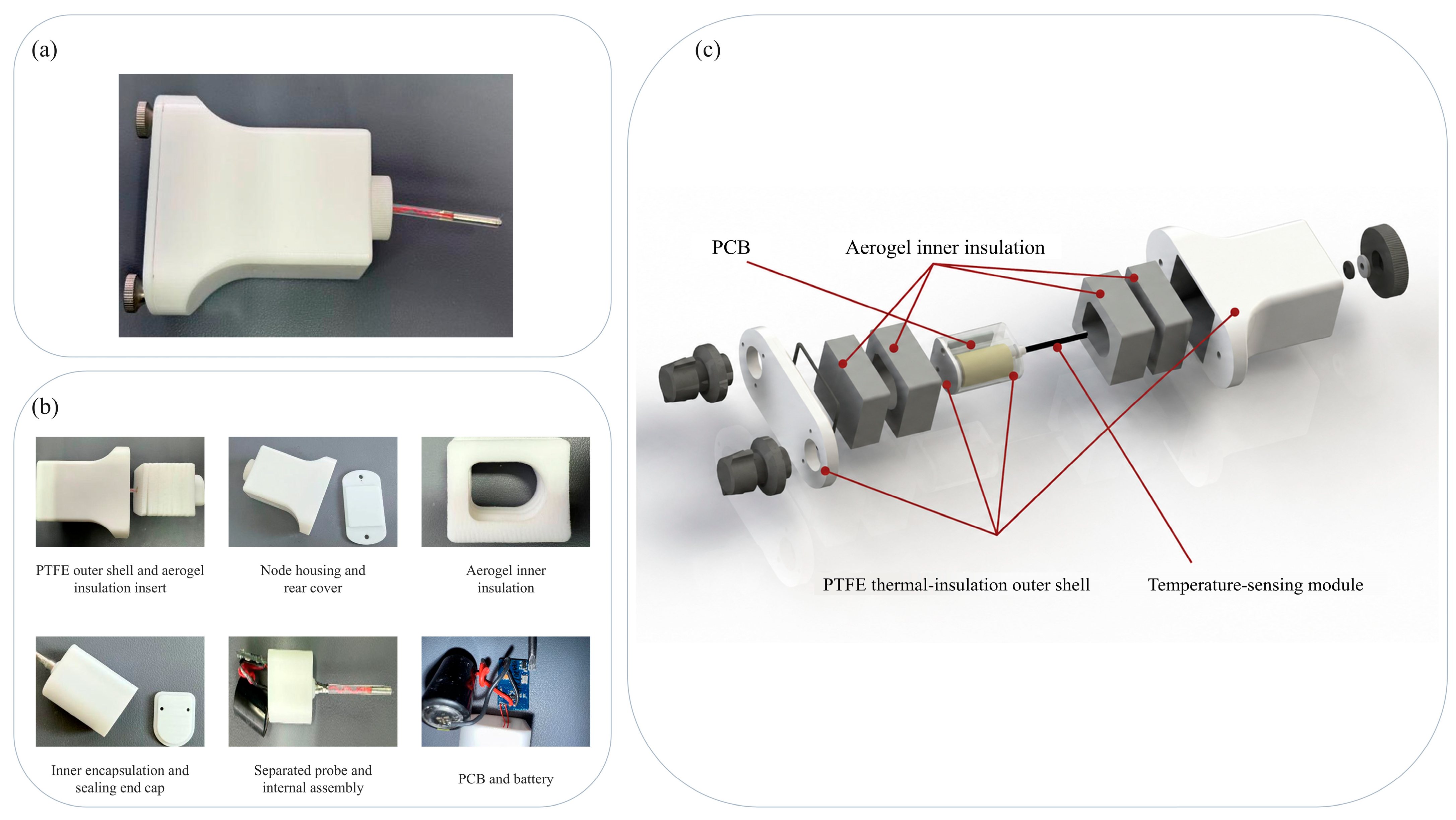
To implement this workflow, the node body comprises a PTFE enclosure, an aerogel insulation sleeve, an inner encapsulation layer, a circuit board, a battery, and an externally mounted remote probe. The battery and circuit board are positioned adjacent to one another inside the insulated body, while the external probe is connected to the acquisition circuit through small-cross-section copper wires. Figure 2 shows the assembled node, the principal components, and the exploded structure.
An Arduino Nano 33 BLE Rev2 controller (Arduino S.r.l., Monza, Italy) coordinates periodic PT1000 sampling, local data buffering and storage, low-power state transitions, and post-warm-up BLE communication. The node also incorporates a low-noise analog front end, a LiFePO4 battery, and a Hall-effect trigger, providing the functional hardware required for the staged sensing workflow.

2.1.3. Multilayer Thermal Protection and Remote Probe

On the insulated-body side, the PTFE enclosure and inner encapsulation provide structural support, while the intermediate aerogel sleeve reduces heat transfer from the internal electronics to the external cryogenic environment. Cryogenic studies have demonstrated the low effective thermal conductivity of aerogels [33,34,35], although their actual thermal response also depends on the density, pore structure, composite configuration, and fabrication process [36,37,38]. The mechanical and thermophysical properties of thermoplastics such as PTFE and polyether ether ketone (PEEK) are likewise temperature-dependent [39,40]. The node design must therefore also account for thermal contraction, assembly clearances, and interfacial contact.
At the sensing end, the PT1000 element is positioned outside the insulated body. A PEEK housing provides mechanical protection, and small-cross-section copper wires provide the electrical connection. Compared with placing the probe entirely inside the main enclosure, this configuration shortens the thermal-response path from the external environment to the sensing element while preventing the battery and circuit board from undergoing the same rapid cooling. Because the copper wires and probe interface still form solid-conduction paths, the remote arrangement does not eliminate heat transfer. Rather, it modifies the distribution of thermal resistance and heat capacity so that the sensing end and the internal electronics cool on different time scales.

2.1.4. Temperature Acquisition, Local Storage, and Low-Power Control

The temperature acquisition chain uses a PT1000 element driven by a two-wire constant-current source. A reference network, differential amplifier, low-pass filter, and an AD7171BCPZ 16-bit low-power sigma-delta analog-to-digital converter (Analog Devices, Inc., Wilmington, MA, USA) condition and digitize the signal. Because lead resistance, self-heating, and probe time constant affect platinum-resistance measurements [23,24,25,26], the excitation source and analog front end are enabled only briefly during each sampling event and switched off after conversion. The controller converts the digitized signal to temperature using the reference resistance, amplification factor, and PT1000 resistance–temperature relationship. The firmware then applies stored conversion, zero, and gain coefficients and lookup-table interpolation. Table 2 reports the measurement ranges, resolution, and supported uncertainty information; Table 3 separately lists the system components and implementation details.
After temperature conversion, each record contains a sample index, temperature value, status flag, and 16-bit cyclic redundancy check (CRC). Records are first written to a static random-access memory (SRAM) buffer. Every 20 records are then written to Flash in a batch and verified by readback. This organization reduces repeated Flash activation and allows the host computer to verify record continuity using the sample indices. To further reduce average power consumption during cryogenic exposure, the system disables the high-speed oscillator and BLE radio and retains only the 32.768 kHz clock for the 5 s timing task. Previous low-power studies have shown that shortening active windows, extending sleep intervals, and reducing communication duty cycles can decrease node energy consumption [18,19,41], consistent with the present design objective of prioritizing acquisition and data retention.

2.1.5. Warm-Up Triggering, BLE Data Retrieval, and Host Software

After the low-temperature task, the node enters the data retrieval stage. It is first allowed to warm naturally at room temperature and is then placed on a trigger platform containing a permanent magnet. When the Hall-effect sensor detects the magnetic field, it wakes the controller, which starts BLE advertising and broadcasts the node identifier. Once a connection has been established, the node reads the stored records sequentially and transmits them in packets. The host software checks each data frame, verification field, and end marker, then reassembles the historical record, displays the temperature curve, and exports the data. The node uses predefined binary record and communication-frame formats. After reassembly, the host application exports the node identifier, sample index, temperature value, status, and verification result as a JavaScript Object Notation (JSON) file for subsequent management and analysis.
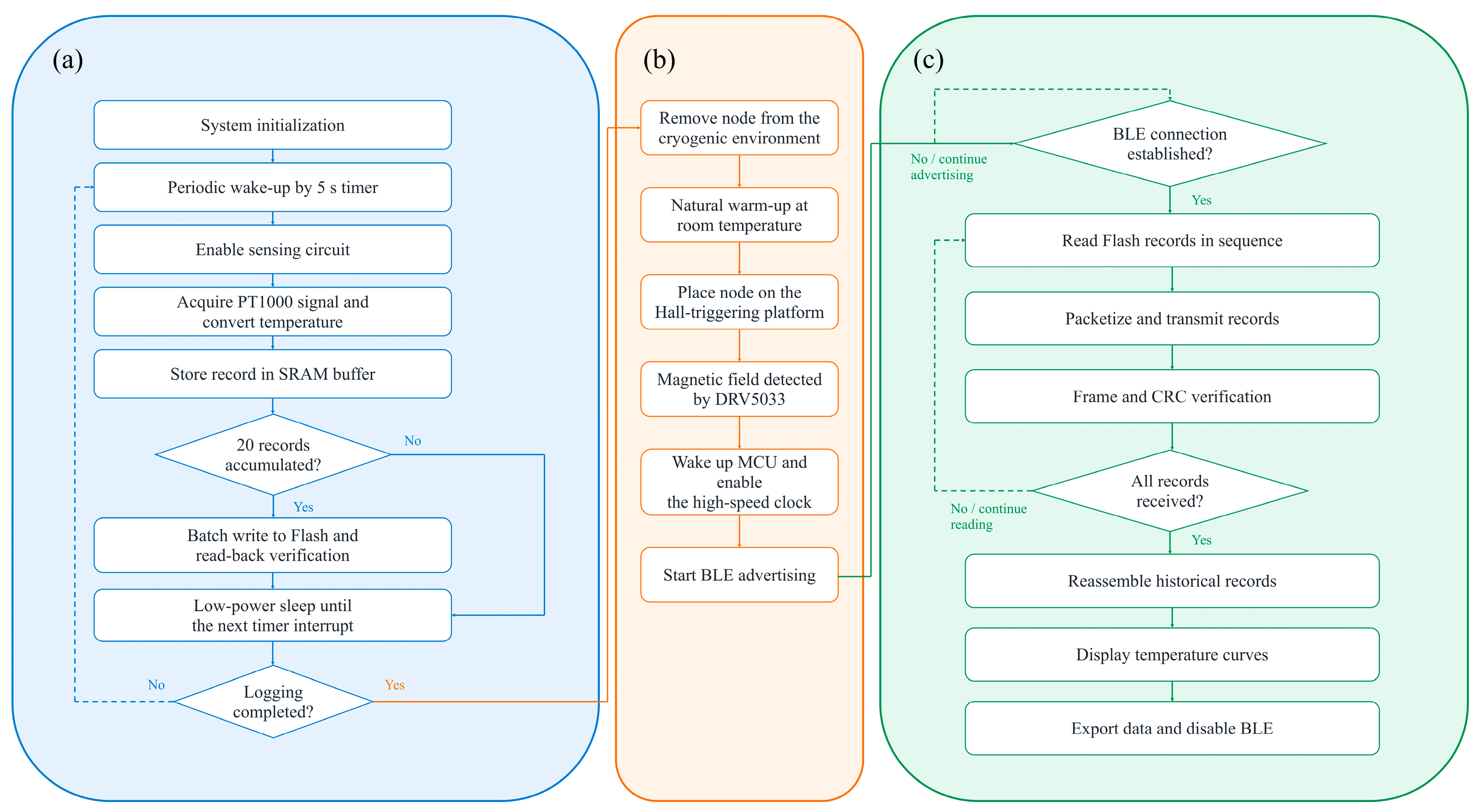
Figure 3 expands the state transitions summarized in Figure 1b. In Figure 3a, initialization establishes the clock, acquisition interface, storage pointers, and interrupts before the controller enters the 5 s sampling loop. Each loop powers the analog front end, acquires and processes the PT1000 signal, appends a verified record to SRAM, writes a 20-record block to Flash when required, and returns the controller to sleep. Figure 3b shows that removal and natural warm-up do not automatically activate the radio; the Hall-effect event provides the explicit wake-up command. Figure 3c shows advertising, connection, sequential packet transmission, frame and CRC verification, retransmission when verification fails, record reassembly, curve display, and export. Thus, each decision symbol identifies a verifiable state transition rather than a separate experimental treatment.

2.2. Numerical Methods

2.2.1. Node Heat-Transfer Model

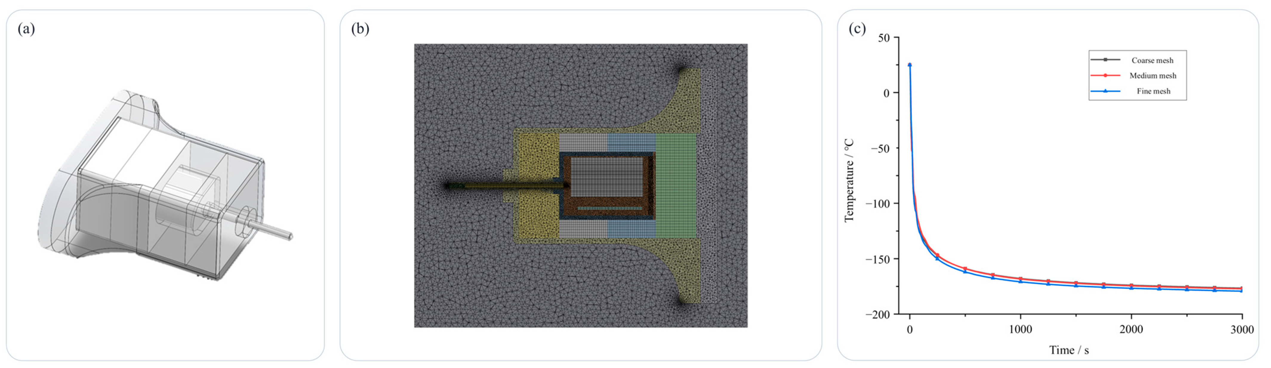
The node model was established to test whether the differentiated thermal path delays cooling of the internal electronics and to interpret the operating-duration results. It includes the PTFE enclosure, aerogel layer, inner encapsulation, PEEK probe housing, copper leads, PT1000 element, circuit board, battery, internal gas, and surrounding cryogenic domain. Retaining nuts, sealing plugs, and small fillets were removed, while the relative positions of the heat-capacity-dominant components and solid-conduction paths were retained. The physical geometry was created in SolidWorks 2025 (Dassault Systèmes SolidWorks Corp., Waltham, MA, USA), simplified and divided into solid and fluid domains in ANSYS SpaceClaim 2024 R2, discretized in ANSYS Meshing 2024 R2, and solved in ANSYS Fluent2024 R2 (ANSYS, Inc., Canonsburg, PA, USA). Figure 4a shows the simplified domains, and Figure 4b identifies the corresponding mesh regions.
The supplied as-designed STEP assembly defines the principal component geometry used in the node model. The combined PTFE-enclosure dimensions (length × width × height) are 70.17 × 70.01 × 39.66 mm, and the envelope dimensions of the complete node, including the remote probe, are 70.17 × 96.77 × 39.66 mm. The PEEK probe housing is 6.00 mm in diameter and 50.00 mm long, of which 26.75 mm projects beyond the enclosure; the sensing-core body is approximately 1.90 mm in diameter and 40.00 mm long. The available archived records provide these component dimensions; the copper-lead and outer-domain dimensions are not separately parameterized. Their numerical representations and the outer-boundary placement were held identical across all three grids, so Figure 4c isolates mesh refinement rather than a change in geometry. Small fasteners, sealing plugs, and fillets were suppressed, and no geometric parameter was fitted to the temperature curve.
Material properties and boundary conditions.
The material properties used in the model are listed in Table 4. Because actual properties vary with temperature, whereas the present model uses fixed values, the parameters are classified into three categories to avoid interpreting them as true properties over the full temperature range. C denotes constant properties used directly in the model, R denotes properties checked at a reference state, and E denotes node-level effective properties obtained by homogenizing complex components. Cryogenic material references and thermophysical property databases were used to check the orders of magnitude and temperature dependence of engineering materials and gases [42,43], while cryogenic studies of aerogels, PEEK, and other polymers were used to check the corresponding parameter ranges [33,34,35,36,37,38,39,40]. Effective properties were assigned to the circuit board and battery to retain their bulk heat capacity and conductive characteristics, following homogenization approaches used in electronic-packaging and battery thermal models [15,44,45].
The node and its internal domains were initialized at 25 °C. For the model evaluation case, the single-point ambient-temperature history recorded beside the evaluation node (Figure 5f) was applied as a time-dependent prescribed temperature at the outer boundary of the cryogenic domain. The internal gas participated in the momentum and energy solutions and exchanged heat with the solid regions through coupled interfaces. No separate thermal contact resistance was assigned at solid–solid interfaces; all contacts were treated as thermally coupled. Gravity acted in the vertical direction. This node-level model does not represent liquid-nitrogen boiling, liquid–gas phase change, or bulk flow within the biobank. Its primary outputs are the temperature histories at the internal PT1000 location, the battery, and the circuit board.
Mesh and Numerical Settings
The mesh was generated in ANSYS Meshing with a 5 mm global target size, a target skewness of 0.75, and the “High” smoothing setting, followed by local refinement of the heat-transfer paths. The PTFE cover used 1 mm tetrahedral elements, while the main PTFE enclosure used a 1 mm automatic mesh. The aerogel layer used 1 mm hexahedral elements; the inner PTFE encapsulation and internal gas used 0.5 mm automatic elements; the circuit board and battery used 1 mm hexahedral elements; the probe housing used 0.5 mm hexahedral elements; the copper leads and PT1000 body used 0.1 and 0.2 mm hexahedral elements, respectively; and the separated probe, interlayer air, and external cryogenic domain used 0.2, 0.2, and 2 mm automatic elements, respectively. Figure 4b uses different colors to identify material domains; the colors do not denote mesh quality. For the selected 2,552,875-cell mesh, the archived mesh-quality report gives a minimum element quality of 0.84, a maximum aspect ratio of 1.83, a maximum skewness of 0.217, and a minimum orthogonal quality of 0.78. Grid independence was evaluated with 1,355,978-cell (coarse), 2,552,875-cell (medium), and 4,395,554-cell (fine) meshes. The medium- and fine-mesh temperature histories nearly overlap throughout the transient test, as shown in Figure 4c. All geometries and boundary placements were held fixed across the three mesh levels. The 2,552,875-cell mesh was selected as the baseline because further refinement produced no visually meaningful change while increasing computational cost.
The numerical workflow followed the explicit sequence SolidWorks CAD → ANSYS SpaceClaim geometry and domain preparation → ANSYS Meshing discretization and quality check → ANSYS Fluent setup and transient solution → extraction of the temperature histories at the internal PT1000, battery, and circuit board. This sequence is consistent with established transient electronic-packaging and conjugate heat-transfer model evaluation workflows [44,45]. A pressure-based transient formulation solved continuity, momentum, and energy with gravity enabled. The Realizable k ′ ε model [46] closed the internal gas-domain momentum equations. Heat conduction in each solid used the conductivity listed in Table 4; gas–solid and solid–solid interfaces were thermally coupled, with no separately fitted contact resistance. Radiative exchange was omitted from the node model. The recorded ambient-temperature history was prescribed at the outer cryogenic-domain boundary, and all internal fluid–solid walls used coupled heat transfer and no slip. The time step was 0.1 s for 35,000 steps (3500 s), with at most 10 inner iterations per step; other numerical controls retained the ANSYS Fluent defaults. Calculations were executed on a 64-bit Windows workstation equipped with an Intel Core i9-14900KF processor and an NVIDIA GeForce RTX 5070 GPU.
Model evaluation method
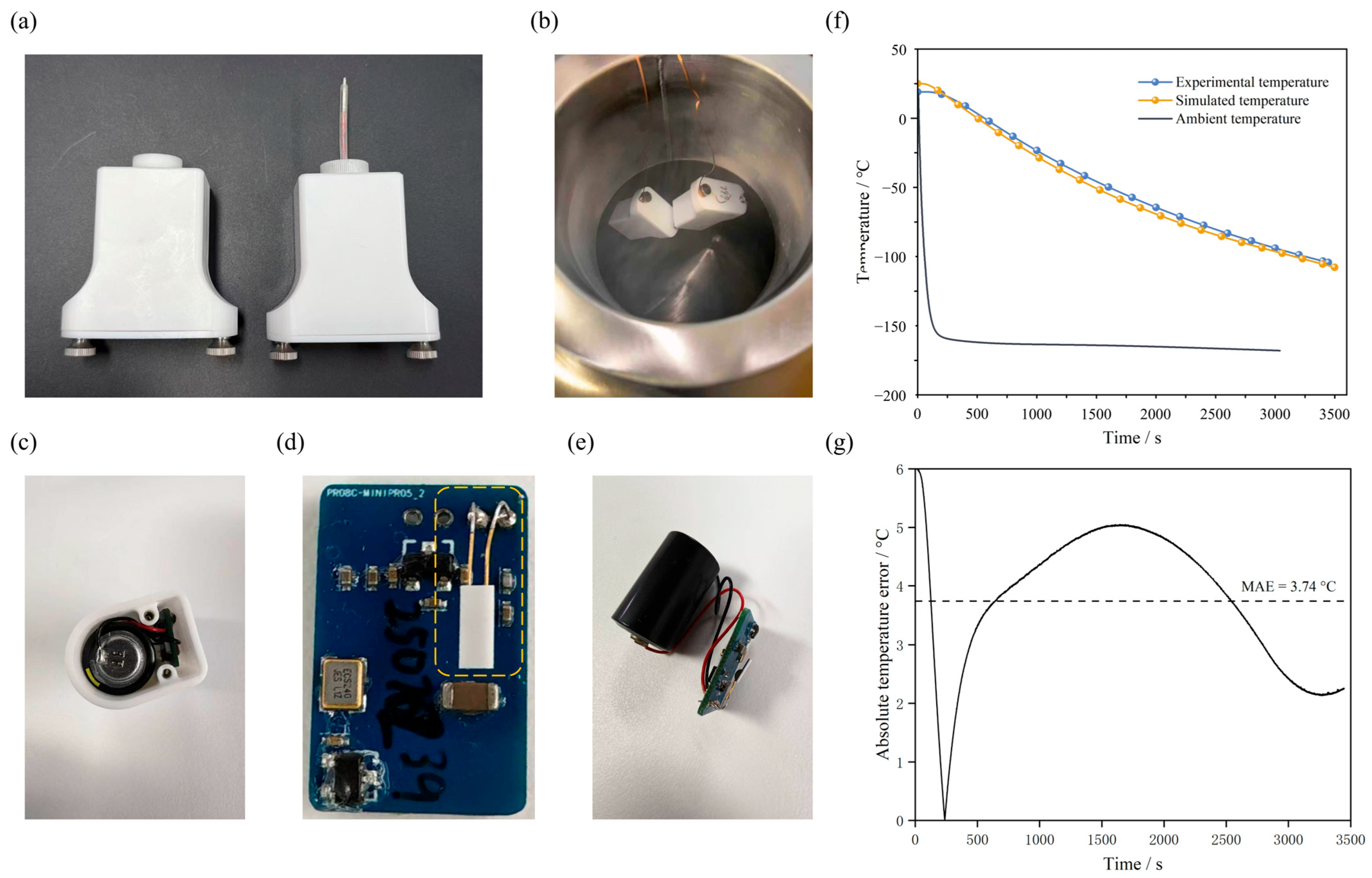
Model evaluation used a dedicated node containing an internal PT1000 above the circuit board and a separate 1 s acquisition channel; the performance and field tests retained the 5 s sampling interval. Figure 5a shows the standard and evaluation nodes; Figure 5b shows the exposure apparatus; and Figure 5c–e show the packaged evaluation node, circuit board, and internal component arrangement, respectively. A standard wireless node was suspended beside the evaluation node at the middle level of the liquid-nitrogen vessel. Its remote PT1000 recorded the single-point ambient history at 5 s intervals, so the ambient trace is not a spatial average. In Figure 5f, lines connect the discrete samples or solver outputs for visual comparison; they do not indicate continuous analog recording. Markers identify the internal experimental samples. The first valid sample defined time zero. The 0.1 s simulation output was sampled at the corresponding 1 s experimental timestamps over the common 0–3446 s interval. Frame and CRC verification and monotonic sample indexing were checked before analysis. The 3447-sample internal record was screened for isolated spikes using adjacent first differences and the residual of each interior sample from the mean of its two neighbors. Adjacent changes ranged from −0.07 to +0.02 °C, and the maximum isolated-point residual was 0.035 °C. For the first differences, the modified score was calculated as 0.6745; the maximum absolute score was 3.37, so no sample exceeded the conventional screening threshold of 3.5. No smoothing, curve fitting, or retrospective sample removal was applied. These checks support the absence of isolated spikes in this record but do not exclude systematic measurement bias or establish the outlier rate of other records. Evaluation is based on one internal record and one adjacent ambient record and therefore assesses trend agreement rather than statistically quantified uncertainty.
Experimental temperature histories are commonly used to evaluate transient conjugate heat-transfer and electronic-packaging models [44,45,47]. Evaluation used three complementary measures. The MAE and RMSE quantify absolute deviations [48]; the Pearson coefficient r describes similarity of the complete time histories; and the first-passage times to −50 °C quantify a practically interpretable timing error. For n aligned points, T s i m , i and T e x p , i denote the simulated and experimental temperatures at time i , respectively:
M A E = 1 n i = 1 n T s i m , i T e x p , i
R M S E = 1 n i = 1 n T s i m , i T e x p , i 2
r = i = 1 n T s i m , i T ¯ s i m T e x p , i T ¯ e x p i = 1 n T s i m , i T ¯ s i m 2 i = 1 n T e x p , i T ¯ e x p 2
The Pearson correlation coefficient was calculated from the simulated and experimental sequences over the overlapping interval. The first-passage time to −50 °C was determined by linear interpolation between the adjacent data points on either side of the threshold. Together, these metrics describe the overall trend, absolute temperature deviation, and timing of a key response event, thereby bounding the model’s applicable range from complementary perspectives.

2.2.2. Biobank Temperature Field Model

The numerical reference curves used for the subsequent field comparisons were extracted from a transient temperature-field model of the liquid-nitrogen biobank developed for this study. This model is independent of the node heat-transfer model described above: the node model explains the thermal response within the package, whereas the biobank model provides reference cooling histories at different spatial locations. The geometry was simplified from the actual vessel while retaining the tank, liquid-nitrogen region, and gaseous storage region. The tank diameter was 1606 mm, the height was 1429 mm, the wall thickness was 10 mm, and the maximum liquid-nitrogen depth was 735 mm. For an approximately 80% loading condition, the gaseous storage region was represented as a porous medium with a porosity of 0.85. The model assumed a closed tank with no-slip walls, neglected heat leakage through the lid seal and radiative heat transfer, treated the liquid nitrogen as an isothermal cold source, and accounted for buoyancy-driven gas flow.
The liquid-nitrogen/nitrogen-gas two-phase flow was represented using the Mixture model [49]. Interphase evaporation and condensation were modeled using the Lee mass-transfer model [50], turbulence closure used the Realizable k − ε model [46], and pressure–velocity coupling used the SIMPLE algorithm [51]. Buoyancy-driven gas flow was treated using the Boussinesq approximation, whose applicability is limited by the magnitude of temperature differences and the associated variation in thermophysical properties [52]. Recent cryogenic CFD studies continue to employ these foundational models. Two-phase and phase-change formulations have been applied to liquid-nitrogen chilldown [53]. A mixture-based approach incorporating the Lee evaporation model has been used to simulate liquid-nitrogen jet evaporation and dispersion [54]. The Realizable k − ε model has also been applied to simulations of liquid-nitrogen flow and temperature distribution in a cryogenic chamber [55]. A recent CFD review has further summarized the theoretical basis, numerical implementation, and applicability of the Boussinesq approximation to buoyancy-driven thermal convection [56]. The liquid-nitrogen temperature, initial gas temperature, and tank-wall temperature were set to −196, −81, and −102 °C, respectively, and a heat flux of 7 W·m−2 was applied to the wall in contact with liquid nitrogen. The coarse, baseline, and refined meshes contained 689,342, 1,237,258, and 3,247,920 cells, respectively. Based on the mesh-independence comparison at representative measurement points, the baseline mesh of 1,237,258 cells was used for the subsequent calculations. The time step was 0.2 s, with 22,000 steps corresponding to a total duration of 4400 s and 20 inner iterations per time step.
The biobank model provides location-specific numerical reference histories, not metrology-grade estimates of absolute temperature. This restriction follows from the porous-medium representation of the stored load, prescribed wall temperatures and heat flux, empirical phase-change parameters, Boussinesq treatment over a large thermal span, omission of lid leakage and radiation, and simplified rack geometry. These assumptions preserve the principal vertical and radial cooling trends but do not reproduce every local obstruction, transient boundary fluctuation, or node-mounting condition. Accordingly, the field comparison evaluates curve shape and level-dependent behavior and does not use the model as a calibration reference.

2.3. Experimental Methods

2.3.1. Experimental Program

The node heat-transfer model was used to interpret the internal cooling process, but experiments were required to verify whether the system could complete the intended engineering workflow. Four tests were therefore conducted in sequence. The effective operating-duration test determined the available logging window in the cryogenic environment; the warm-up reconnection test evaluated connection recovery after node removal; the indoor BLE distance test examined the distance dependence of historical data retrieval; and the operating-biobank deployment test evaluated multi-location temperature logging. All four tests used the developed nodes, trigger unit, and host computer. The internal PT1000 data described in Section 2.2.1 were used solely for model evaluation and were not combined with the system performance data.
The developed node, Hall-effect trigger, and host computer were functional parts of the system rather than independent reference instruments. Both temperature channels in Figure 5f used the developed PT1000 acquisition chain reported in Table 2. The internal channel was installed above the evaluation-node circuit board, while the ambient channel was the remote PT1000 of the adjacent standard node. The 3447-sample internal record covered an observed interval from −104.26 to 19.06 °C. The AD7171BCPZ provides a 16-bit output, and temperatures were exported in 0.01 °C increments. These documented quantities define the evaluated record and the engineering-performance claims; they do not by themselves establish traceable measurement accuracy.

2.3.2. Uncertainty Treatment

Uncertainty was quantified only where the archived evidence supported a numerical estimate. For a recorded quantity with a least significant increment q , assuming a rectangular distribution, the standard uncertainty associated with quantization was calculated as:
u q = q 12
Accordingly, the individual resolution-related standard uncertainty components were 0.0029 °C for temperature values rounded to 0.01 °C, 0.29 s for timestamps recorded at 1 s intervals, 1.44 s for timestamps recorded at 5 s intervals, and 1.44 min for the 5 min warm-up observation grid. These values represent individual resolution components rather than complete system-level uncertainties.
For the mean operating duration of the nine nodes, the Type A contribution arising from between-node variation was calculated as:
u A = s n
where s = 2.87 min is the between-node sample standard deviation and n = 9 is the number of nodes. This contribution was combined with the standard uncertainty associated with the 5 s timestamp interval:
u c = u A 2 + u t 2 = s n 2 + 5 / 60 12 2 = 0.96   m i n , k = 1 .
This combined standard uncertainty characterizes the reported group mean rather than the repeated-use uncertainty of an individual node. A combined standard temperature uncertainty in the Guide to the Expression of Uncertainty in Measurement (GUM) sense could not be reconstructed because the experimental campaign did not include a traceable system-level calibration or a complete uncertainty budget covering the PT1000 element, lead wires, excitation source, analog front end, and conversion coefficients. In addition, each field location was measured once. Therefore, the temperature figures present the measured traces and model-discrepancy statistics without unsupported uncertainty bars. Model residuals and between-node variations are reported separately and are not interpreted as instrument uncertainty.

2.3.3. Effective Operating-Duration Test

The effective operating-duration test included all nine fully assembled and functional nodes available for the test campaign; they were not selected as a statistical subset. Their physical identifiers were 702, 723, 730, 754, 774, 784, 799, 938, and 988. For concise presentation, these identifiers are mapped to N1-N9 in the same order in the reported results. After initialization and functional checks, each node was placed at a predetermined liquid-nitrogen biobank location, sampled every 5 s, and wrote records to Flash with BLE disabled. After removal, warm-up, and data export, effective operating duration was defined as the timestamp of the final record that passed frame verification and could be parsed in sequence. One complete record was obtained from each node. The mean, median, sample standard deviation, range, and coefficient of variation were calculated; the sample standard deviation describes between-node dispersion, not repeat-test uncertainty for an individual node.

2.3.4. Warm-Up and Reconnection Test

After cryogenic exposure, the nine nodes were allowed to warm naturally in an indoor environment at approximately 25 °C. Observations were made at 5, 10, 15, 20, 25, 30, 35, and 40 min, and the number of nodes that successfully established a BLE connection was determined from the trigger and connection records at each time point. The number of successfully connected nodes was used as a system-level recovery indicator for the chain comprising battery power delivery, microcontroller startup, Hall-effect trigger recognition, and BLE communication. Completion of the entire historical data transfer was not included in the success criterion for this test.

2.3.5. Indoor BLE Communication-Distance Test

After connection recovery, an engineering test of BLE retrieval distance was conducted indoors under conditions with limited obstruction and interference. One node that had warmed up and could connect normally was used to execute the same historical-data retrieval procedure at distances of 2, 4, 6, 8, 10, 12, 14, and 16 m. The packet-loss rate (PLR) was defined as follows:
P L R = N s e n t N r e c e i v e d N s e n t × 100 %
where N s e n t is the number of packets transmitted by the node, and N r e c e i v e d is the number successfully received by the host computer. The packet-loss rate at each distance was calculated from the transmitted and received packet counts stored by the system. This test was intended as an engineering screening of distance effects for the present hardware and indoor arrangement; it was not intended to establish a general propagation model or statistical confidence interval.

2.3.6. Operating Biobank Deployment and Numerical Comparison

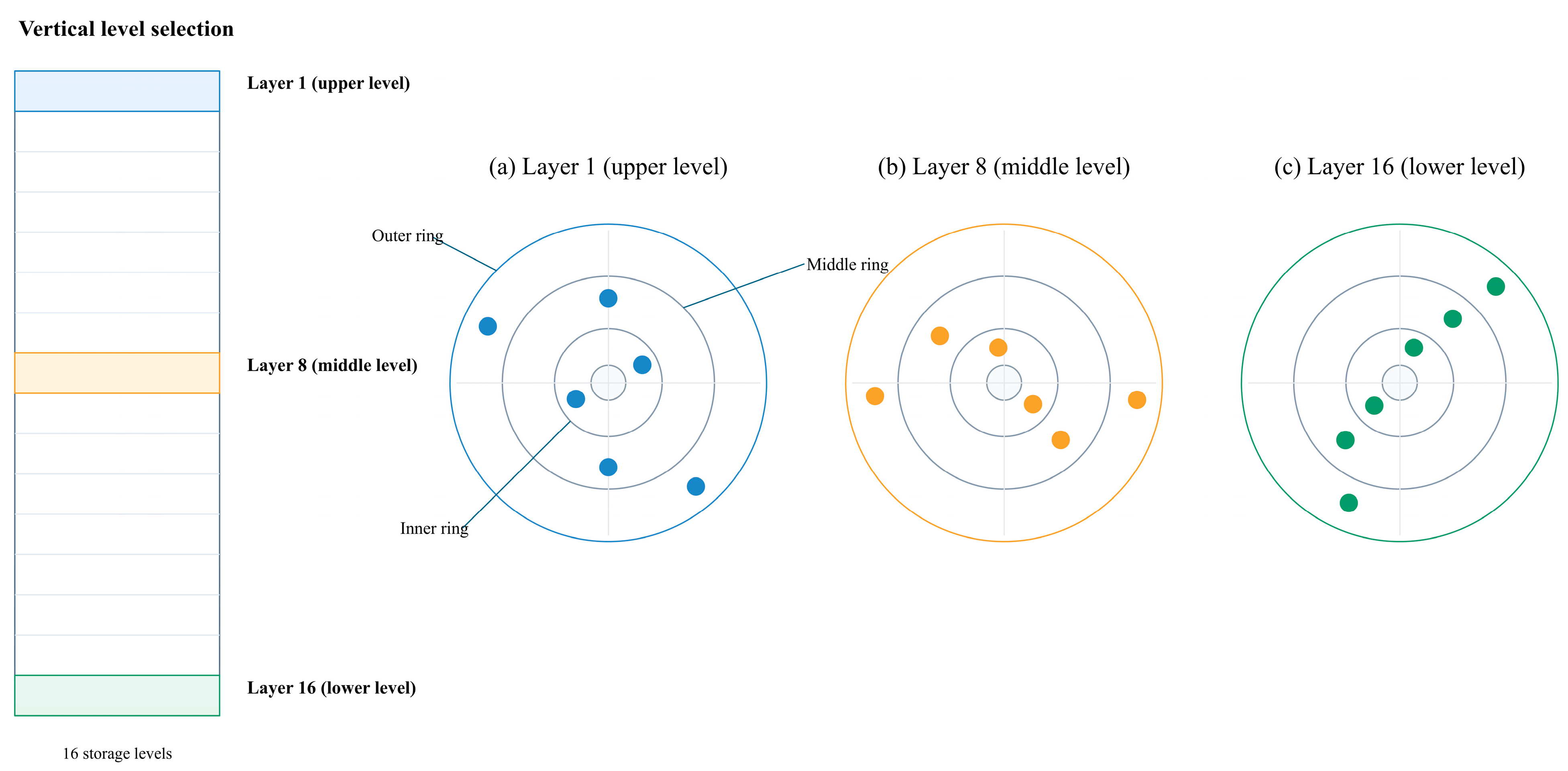
Finally, the system was deployed in an operating liquid-nitrogen biobank to determine whether the preceding design and tests could support a complete field workflow. Layers 16, 8, and 1 were selected along the vertical direction to represent the lower, middle, and upper levels, respectively. At each level, two locations were selected in each of the inner, middle, and outer rings, giving six locations per level and eighteen planned measurement locations in total. Each location was identified by a rack-column number X and a layer number Y; for example, X09Y16 denotes Layer 16 in rack column 09. Figure 6 illustrates coverage of the three vertical levels and three radial rings. The schematic indicates the spatial arrangement only and does not represent exact angles or geometric proportions.
The measurement locations were tested sequentially. Each node sampled temperature every 5 s and wrote the data to on-chip Flash, with wireless communication disabled during cryogenic exposure. At the end of the scheduled test interval, the node was removed, allowed to warm naturally at room temperature, triggered by the Hall-effect unit, connected through BLE, and used to retrieve the historical data. The numerical curve for each location was extracted from the biobank temperature-field reference model described in Section 2.2.2 and assigned the same X–Y identifier as the field location. The measured and numerical curves were each shifted so that their own first record defined time zero. The comparison was used to examine temporal trends rather than reconstruct the full temperature field at a common instant, and the reference-model parameters were not fitted to the field curves.

3. Results and Discussion

This section first evaluates the node thermal response, then reports operating duration, warm-up reconnection, and BLE retrieval distance, and finally compares measured and numerical reference histories at the lower, middle, and upper biobank levels. The final subsection defines the intended use and limitations of the system and both numerical models.

3.1. Node Thermal Response and Model Evaluation

Figure 5f compares the internal PT1000 measurement, the simulated internal temperature, and the single-point ambient record, and Figure 5g shows the corresponding absolute error. The experimental and simulated internal curves both decreased continuously and progressively flattened. After aligning the 0.1 s simulation output with the 1 s experimental timestamps over 0–3446 s, the MAE was 3.74 °C, the RMSE was 3.92 °C, and r was 0.9986. The signed residual (simulation minus experiment) had a mean of −3.23 °C and a standard deviation of 2.22 °C. The measured and simulated curves first crossed −50 °C at 1607.2 and 1483.7 s, respectively, giving a 123.5 s timing difference. The absolute error remained at or below 6.02 °C over the evaluated interval. Relative to the observed experimental span of 123.32 °C, the MAE and RMSE correspond to 3.03% and 3.17%, respectively. The high correlation indicates similarity in curve shape, while the residual statistics, MAE, RMSE, absolute-error curve, and threshold-time difference quantify the remaining temperature and response-time discrepancies. These model-discrepancy statistics are not a substitute for measurement uncertainty. The spike screen described in Section 2.2.1 found no isolated discontinuity in the 3447-point internal record; this continuity check does not rule out systematic measurement bias.
These metrics show that the model captures the overall decrease in internal node temperature but does not reproduce every local temperature or response event exactly. The high correlation coefficient primarily reflects the common direction and shape of the two monotonic cooling curves, whereas the RMSE and threshold-time difference reveal the remaining absolute discrepancy. The three-level mesh comparison reduces the concern that this discrepancy is dominated by grid resolution. More likely sources include simplification of the local external cryogenic boundary, constant and component-level effective properties, the treatment of interfacial contact, and the identification of the exposure start. The internal node temperature lagged substantially behind the external cryogenic environment, consistent with the combined thermal resistance of the cryogenic insulation and multilayer package [33,34,35]. Published transient electronic-packaging and conjugate heat-transfer studies likewise use experiment-model histories to evaluate dynamic temperature response [44,45,47]. Their numerical errors are not used as a direct benchmark here because the geometries, thermal boundaries, sensors, and temperature ranges differ from those of the present cryogenic node. Because PTFE, aerogel, and contact interfaces were not varied independently, their separate contributions cannot be quantified. The model is therefore suitable for interpreting the overall thermal response and comparing the cooling of key components but not for metrology-grade temperature prediction.

3.2. Effective Operating Duration

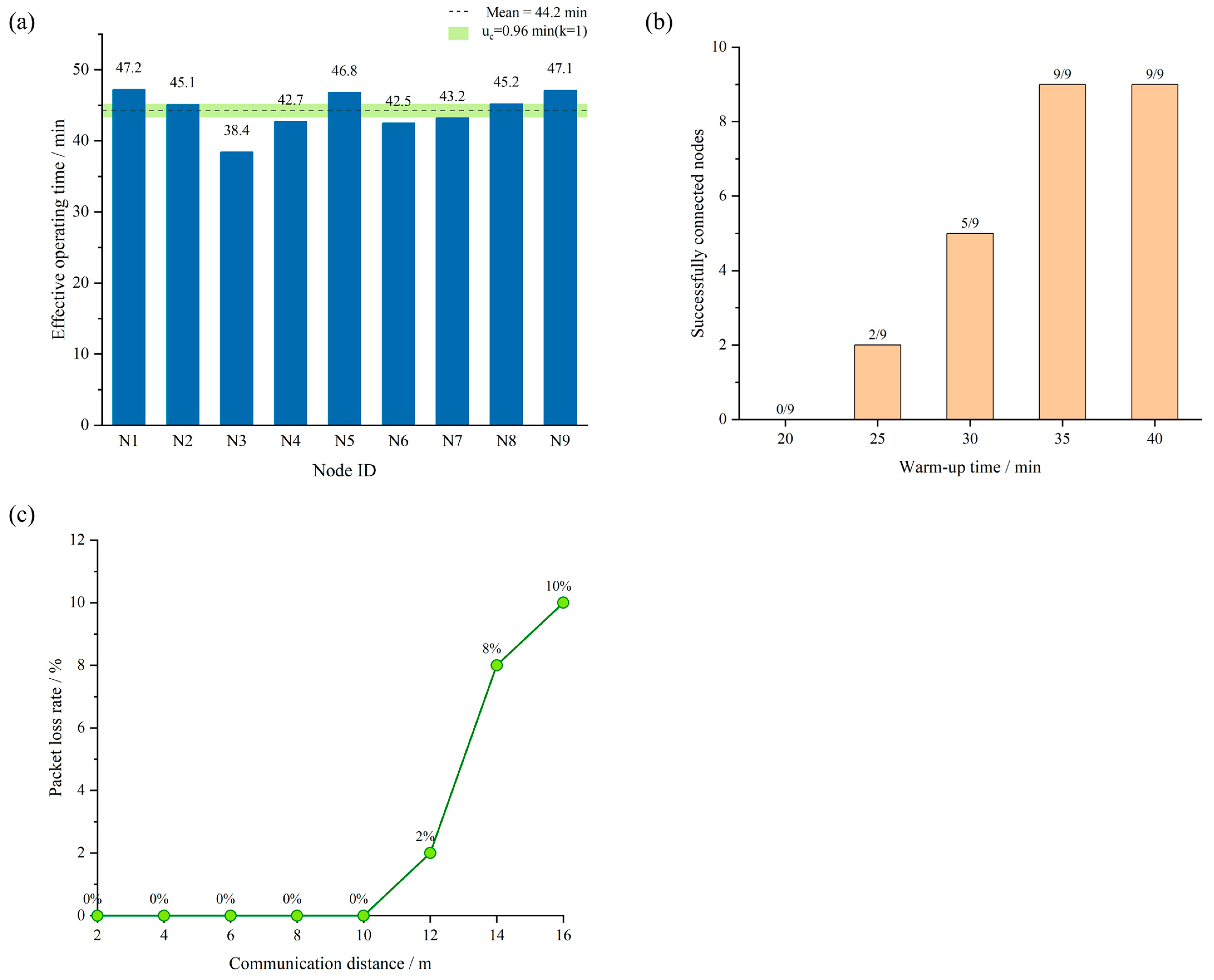
The thermal-response analysis demonstrated a lag in internal cooling, but whether this lag provides a usable logging window must be determined experimentally. Figure 7a and Table 5 show that the effective operating durations of the nine nodes ranged from 38.4 to 47.2 min, with a mean of 44.2 min and a between-node sample standard deviation of 2.87 min. Combining the Type A standard uncertainty of the mean with the 5 s timestamp-quantization component gives u_c = 0.96 min (k = 1); this interval is shown as the shaded band in Figure 7a. The sample standard deviation describes dispersion among nodes and is not repeated-measurement uncertainty for an individual node. Under the present exposure task and 5 s sampling strategy, the nodes therefore sustained temperature acquisition and local storage for several tens of minutes.
The operating duration varied among nodes, potentially because of differences in aerogel assembly, enclosure sealing, internal contact, initial battery state, deployment location, and individual components. Low-temperature changes in transport, impedance, and available capacity of LiFePO4 batteries affect node power delivery [13,14,15,16,57], but the present test evaluated the complete node rather than the electrochemical performance of an isolated cell. In the system design, the remote probe provides a rapid response to the external temperature, while the insulated body and low-duty-cycle strategy delay cooling of the internal electronics and reduce energy consumption. The current experiments do not resolve the relative contribution of each factor, but the results show that their combined effect supports finite-duration cryogenic logging.

3.3. Warm-Up Reconnection

After low-temperature logging, the connection must recover during warm-up before the stored historical data can be retrieved. Figure 7b shows the number of nodes that established a connection at each observation time from 20 to 40 min. The result was 0/9 at 20 min and 2/9, 5/9, 9/9, and 9/9 at 25, 30, 35, and 40 min, respectively. The results at 5, 10, and 15 min were also 0/9 and were omitted from the figure because they duplicated the 20 min result. Connection recovery was therefore strongly time-dependent. For the present node configuration, approximately 25 °C environment, and test procedure, all nine nodes had established BLE connections by 35 min.
The output capability of LiFePO4 batteries is strongly temperature-dependent [13,14,15,16,17,57], so recovery of the power supply may contribute to this behavior. However, connection establishment also depends on microcontroller startup, Hall-effect trigger recognition, and BLE communication, and the 35 min result cannot be attributed to a single battery mechanism. Nor does this time imply that all historical data have been transferred; rather, it provides an empirical waiting period before initiating wireless retrieval after the low-temperature logging stage.

3.4. BLE Communication

Following connection recovery, Figure 7c and Table 5 present the packet-loss rates measured at different retrieval distances. No packet loss was observed from 2 to 10 m in the indoor engineering test, while loss rates of 2%, 8%, and 10% were recorded at 12, 14, and 16 m, respectively. BLE received signal strength and effective coverage depend on distance, obstructions, the propagation environment, and device arrangement [21,22], while packet loss is also affected by connection parameters, buffering, platform behavior, and retransmission mechanisms [58]. These results define the short-range retrieval capability of the present system under the specified indoor arrangement and should not be interpreted as general BLE link-performance parameters.
Because wireless data retrieval occurs after the node has been removed from the cryogenic environment, the host computer can be positioned near the node. The tested range of 2–10 m therefore covers the intended short-range historical-data retrieval scenario. These results apply only to the present hardware and indoor arrangement; they do not indicate real-time BLE performance inside a metal vessel or performance under severe obstruction and interference.

3.5. Measured and Numerical Reference Temperature Histories at Different Biobank Levels

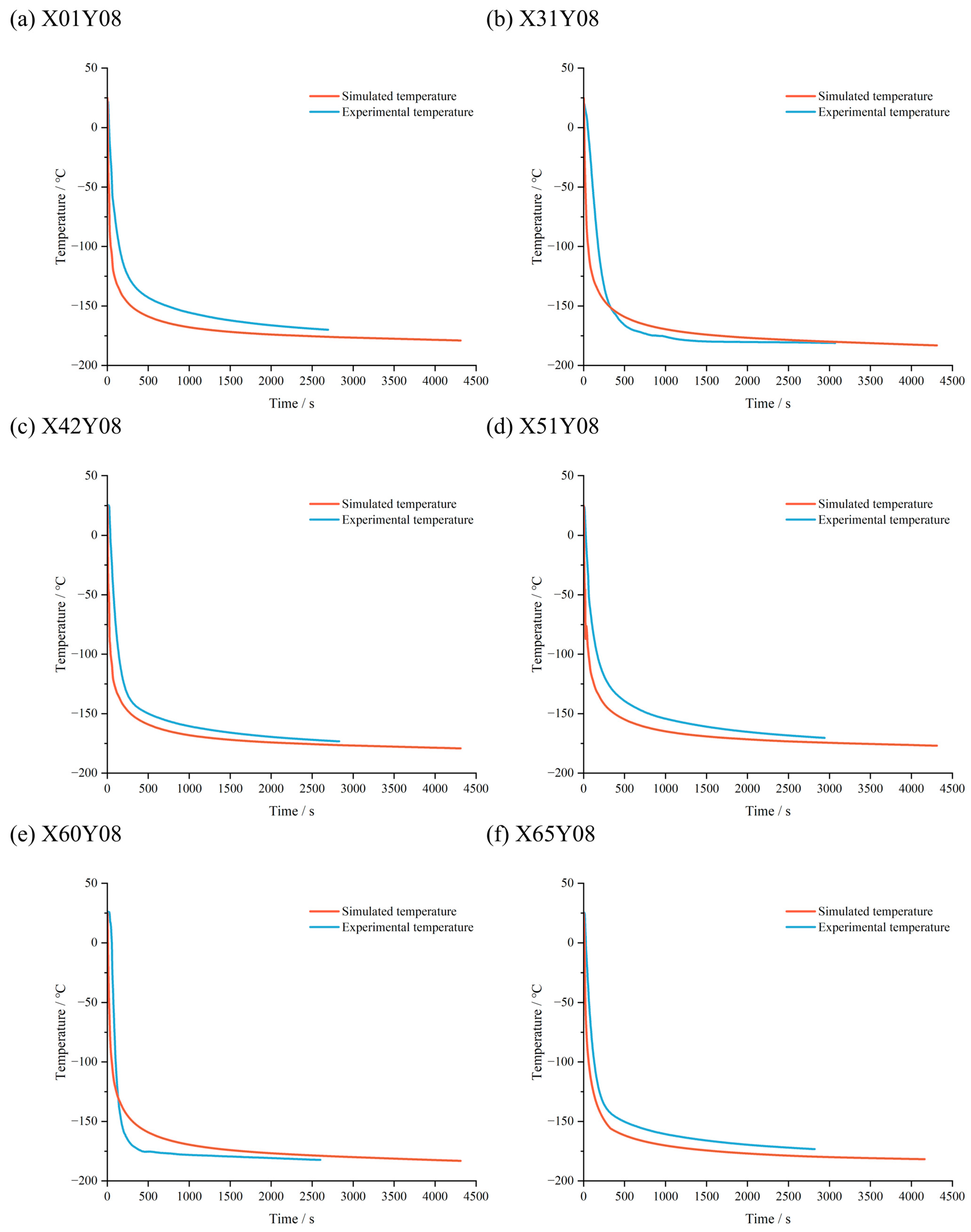
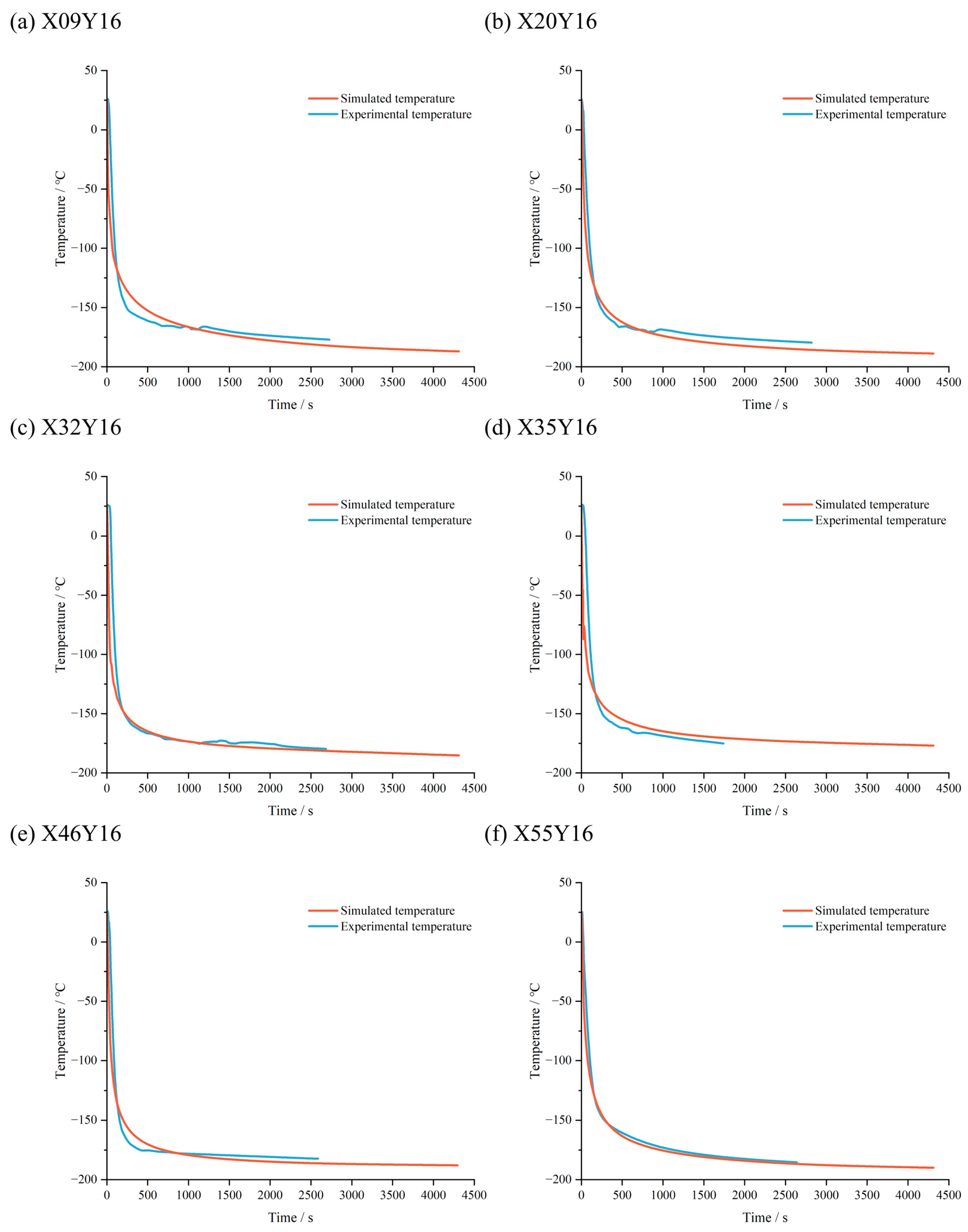
Figure 8, Figure 9 and Figure 10 show the measured and numerical reference temperature histories at six locations on Layers 16, 8, and 1, respectively. All 18 measured curves exhibit a distinctly nonlinear cooling process, with an initially rapid decrease followed by a progressively lower cooling rate. Because the locations were tested sequentially, each location had one record, and the numerical model used idealized boundaries and spatial homogenization, the comparison focuses on curve shape and level-dependent differences. It does not reconstruct the full temperature field at a common instant, nor are metrology-oriented error metrics or Type A temperature uncertainty calculated collectively for all 18 curves. The absence of a numerical combined temperature-uncertainty band is stated explicitly in the captions and Table 2 rather than replaced by model residuals or between-location variation.
At the six lower-level locations in Figure 8, the measured and numerical reference curves show broadly similar shapes during both the rapid-cooling and later deceleration stages. The two curves at X32Y16 and X55Y16 remain relatively close over most of the recorded interval. At X09Y16, X20Y16, X35Y16, and X46Y16, local differences appear in the early response rate or in the mid- to late-stage temperature level. Compared with the middle and upper levels, the lower-level locations show relatively stronger overall trend agreement, suggesting more stable cooling closer to the cryogenic source. Nevertheless, node mounting, local cold-gas pathways, and the actual boundary conditions still influence the temperature history at an individual location.
The six middle-level locations in Figure 9 retain the overall transition from rapid cooling to a gradually stabilizing response, but the relationship between the measured and numerical reference curves is more location-dependent. At X01Y08, X42Y08, X51Y08, and X65Y08, the measured temperatures exceed the numerical reference temperatures over most of the recorded interval, indicating a relatively slower field cooldown. At X60Y08, the measured curve lies below the numerical reference curve during the rapid-cooling stage, indicating faster field cooling at that location. X31Y08 shows an early lag followed by gradual convergence and a short interval in which the measured temperature falls below the numerical result. These differences indicate that the middle-level temperature response is more sensitive to the combined effects of local gas-flow paths, rack structure, and node placement. Because no strictly synchronized environmental baseline was available, the differences are not attributed to a single heat-transfer mechanism.
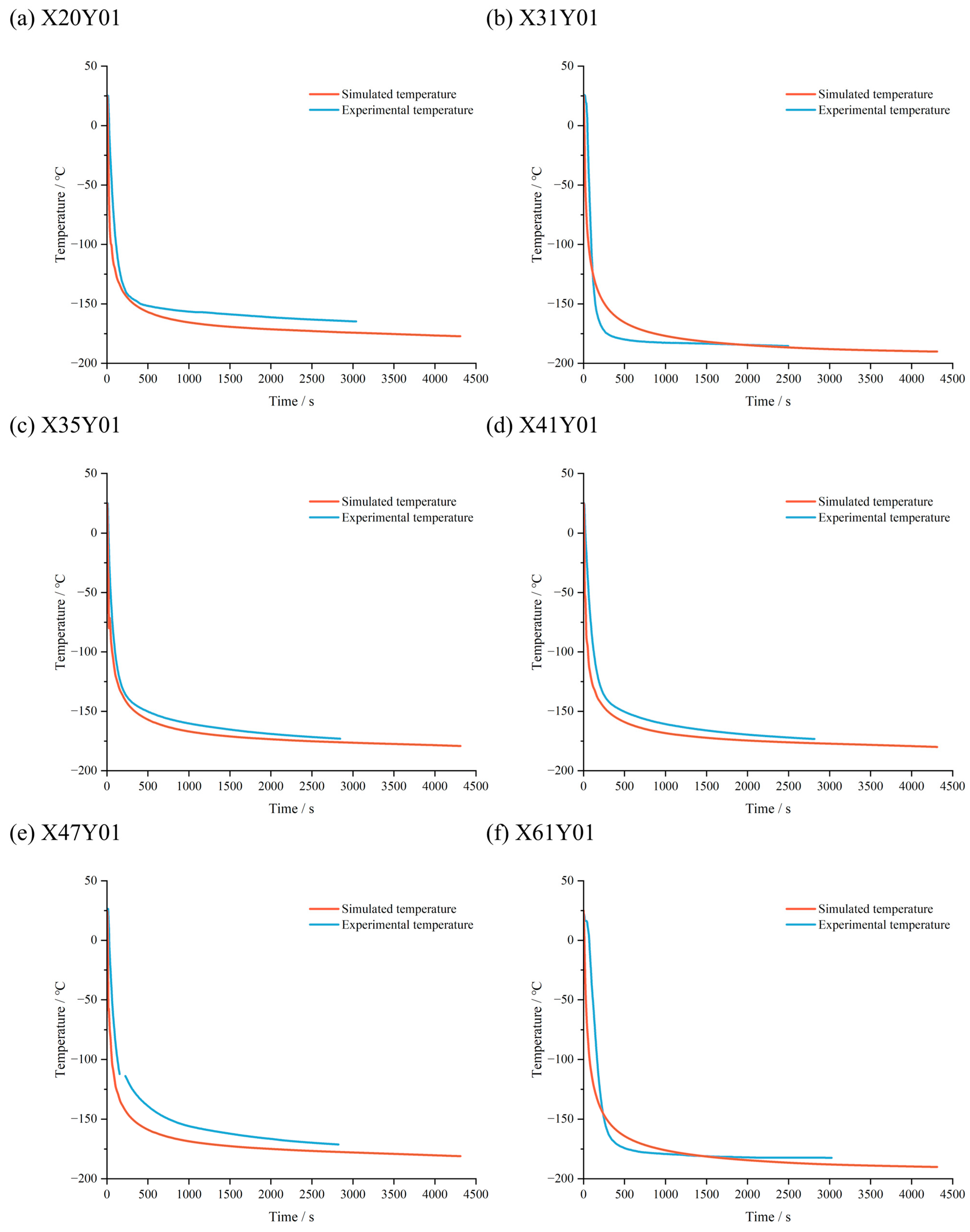
All six upper-level locations in Figure 10 undergo rapid cooling followed by a progressively slower response, but the relationship between the measured and numerical reference curves is strongly location-dependent. At X20Y01, X35Y01, X41Y01, and X47Y01, the measured temperatures remain above the numerical reference temperatures over most of the middle and later intervals, indicating a relative delay in field cooling. At X31Y01, the measured temperature is substantially lower than the numerical reference temperature during the early rapid-cooling stage and then gradually converges. At X61Y01, the measured curve initially cools faster and subsequently approaches, and locally exceeds, the numerical reference result. Because the upper level is farther from the liquid-nitrogen region, its temperature response is more readily affected by upward transport and diffusion of cold gas, local structural obstruction, and node mounting location. The idealized model therefore has limited ability to describe the absolute temperature at a specific upper-level location. The comparison is used to identify overall trends and spatial nonuniformity rather than to claim pointwise predictive accuracy.

3.6. Intended Use and Study Limitations

The system addresses diagnostic temperature-history logging, not real-time protection. Fixed cryogenic sensors and the biobank control system must remain responsible for alarms and corrective action when temperature leaves the target range. Passive backscatter and resonant indicators reduce or eliminate cryogenic-side battery demand and are suitable for interrogation or threshold-state logging [28,29,30,31]. Continuously online nodes provide immediate data but require sustained power and communication [18,19,41], whereas delay-tolerant architectures transfer accumulated records when a link becomes available [32]. The present battery-powered node postpones BLE retrieval until after warm-up. It preserves the finite-duration history but cannot provide an alarm or alter the cooling or heating process during exposure.
Accordingly, the system is best suited to short-duration temperature-history logging, operating-condition assessment, and tests at selected locations. The comparisons at the 18 locations in Figure 8, Figure 9 and Figure 10 further demonstrate that the system can recover dynamic temperature histories from different vertical levels, although local differences remain affected by spatial nonuniformity within the biobank and by model simplifications. In extremely low-temperature environments, the node provides only a logging window on the order of tens of minutes, and the stored data must be retrieved after warm-up.
In addition, the node heat-transfer model uses constant and component-level effective properties, does not independently calibrate thermal contact resistance, and does not include a turbulence-closure sensitivity analysis. The biobank temperature-field model applies the Boussinesq approximation, prescribed boundaries, and a porous-medium representation, so its local temperatures are used only as trend references. The study does not report a traceable system-level temperature calibration, repeated measurements at each field location, or a complete temperature uncertainty budget. Consequently, the 0.0029 °C output-rounding component is not presented as the combined system uncertainty, and model residuals are not used as measurement error bars. The conclusions are restricted to the engineering workflow comprising acquisition, storage, warm-up reconnection, historical data retrieval, and multi-location deployment and are not extended to long-term online monitoring or metrology-grade absolute-temperature measurement.

4. Conclusions

A reusable system comprising wireless temperature-sensing nodes, a Hall-effect trigger, and a host computer completed the intended sequence of cryogenic acquisition, local storage, natural warm-up, triggered BLE connection, and historical data retrieval. The design deliberately exchanges real-time availability for a finite logging window and lower radio demand during cryogenic exposure.
The remote PT1000 and PTFE/aerogel body created different thermal-response paths for the sensing end and internal electronics. The node model reproduced the overall cooling shape (r = 0.9986), with an MAE of 3.74 °C, an RMSE of 3.92 °C, and a 123.5 s difference in reaching −50 °C. The three-level grid study supported the use of the 2,552,875-cell mesh. Together, the quantified experiment–model agreement and grid-convergence evidence support use of the model for physical interpretation and component-level cooling comparison under the stated assumptions. Metrology-grade absolute-temperature certification remains outside the present scope.
The effective operating durations of the nine nodes ranged from 38.4 to 47.2 min, with a mean of 44.2 min, a between-node sample standard deviation of 2.87 min, and a combined standard uncertainty of the mean of 0.96 min (k = 1). The present structure and 5 s sampling strategy therefore support cryogenic logging for several tens of minutes. After 35 min of warm-up at approximately 25 °C, all nine nodes established BLE connections, providing an empirical waiting time before initiating wireless retrieval after low-temperature logging.
Historical data retrieval showed no packet loss from 2 to 10 m in the tested indoor arrangement; loss increased to 2%, 8%, and 10% at 12, 14, and 16 m. All 18 planned field locations across Layers 16, 8, and 1 yielded retrievable temperature histories. Agreement with the numerical reference curves was strongest in overall shape and was more location-dependent at the middle and upper levels. The system is therefore suitable for short diagnostic surveys and workflow assessment at selected locations. It should be used alongside, not in place of, validated fixed sensors for alarms, long-term monitoring, or temperature control.

Author Contributions

Conceptualization, X.L., X.Z. and X.X.; methodology, X.L., T.Z., Z.X. and X.X.; software, X.L.; validation, X.L., J.C. and Z.X.; formal analysis, X.L. and Z.X.; investigation, X.L., T.Z. and J.C.; data curation, X.L. and J.C.; visualization, X.L.; writing—original draft preparation, X.L.; writing—review and editing, T.Z., J.C., Z.X., X.Z. and X.X.; resources, T.Z., J.C. and Z.X.; supervision, X.Z. and X.X.; project administration, J.C., Z.X. and X.Z.; funding acquisition, J.C., Z.X. and X.Z. All authors have read and agreed to the published version of the manuscript.

Funding

This work was supported by the Scientific Research Project of Chengdu Institute of Metrological Verification and Testing (Grant No. 2025CDJL002) and by the Project Committee of Shanghai Institute of Measurement and Testing Technology Co., Ltd., China (Grant Nos. G00RY2505 and P00RY2601).

Data Availability Statement

The data supporting the findings of this study, including node performance-test records, field temperature histories, and model-comparison data, are available from the corresponding author upon reasonable request.

Conflicts of Interest

Author Tianyu Zhu was employed by Beijing Lindian Weiye Electronic Technology Co., Ltd. Author Zhichun Xiong was employed by Shanghai Institute of Measurement and Testing Technology Co., Ltd. The authors declare that this research was conducted in the absence of any commercial or financial relationships that could be construed as a potential conflict of interest. The funders had no role in the design of the study; in the collection, analyses, or interpretation of data; in the writing of the manuscript; or in the decision to publish the results.

References

  1. Graham, M.; Samuel, G.; Farley, M. Roadmap for low-carbon ultra-low temperature storage in biobanking. J. Transl. Med. 2024, 22, 747. [Google Scholar] [CrossRef] [Scilit] [PubMed]
  2. Khaydukova, I.V.; Ivannikova, V.M.; Zhidkov, D.A.; Belikov, N.V.; Peshkova, M.A.; Timashev, P.S.; Tsiganov, D.I.; Pushkarev, A.V. Current State and Challenges of Tissue and Organ Cryopreservation in Biobanking. Int. J. Mol. Sci. 2024, 25, 11124. [Google Scholar] [CrossRef] [Scilit] [PubMed]
  3. Zeng, X.; Chen, Y.; Sehrawat, A.; Lee, J.; Lafferty, T.K.; Kofler, J.; Berman, S.B.; Sweet, R.A.; Tudorascu, D.L.; Klunk, W.E.; et al. Alzheimer blood biomarkers: Practical guidelines for study design, sample collection, processing, biobanking, measurement and result reporting. Mol. Neurodegener. 2024, 19, 40. [Google Scholar] [CrossRef] [Scilit] [PubMed]
  4. Weikert, J.; Mehrländer, A.; Baber, R. Keep cool! Observed temperature variations at different process stages of the biobanking workflow—Examples from the Leipzig medical biobank. J. Lab. Med. 2023, 47, 69–80. [Google Scholar] [CrossRef] [Scilit]
  5. Kim, K.; Kang, M.S.; Huh, J. Effect of Exposure to Room Temperature During Storage on Cryopreserved Umbilical Cord Blood Quality. Ann. Lab. Med. 2026, 46, 110–114. [Google Scholar] [CrossRef] [Scilit] [PubMed]
  6. Catterson, P.J.; Olson, T.T.; Penno, M.B.; Callahan, S.P.; Olson, M.V. Indicator Tubes: A Novel Solution for Monitoring Temperature Excursions in Biobank Storage. Methods Protoc. 2025, 8, 120. [Google Scholar] [CrossRef] [Scilit] [PubMed]
  7. Linsen, L.; Van Landuyt, K.; Ectors, N. Automated Sample Storage in Biobanking to Enhance Translational Research: The Bumpy Road to Implementation. Front. Med. 2020, 6, 309. [Google Scholar] [CrossRef] [Scilit] [PubMed]
  8. Shin, M.; Hwang, S.; Kim, B.; Seo, S.; Kim, J. IoT-Based Intelligent Monitoring System Applying RNN. Appl. Sci. 2022, 12, 10421. [Google Scholar] [CrossRef] [Scilit]
  9. Lee, W.S. A Low-Cost Cryogenic Temperature Measurement System Using Arduino Microcontroller. Phys. Educ. 2020, 55, 023002. [Google Scholar] [CrossRef] [Scilit]
  10. Liu, Z.; Tian, B.; Jiang, Z.; Li, S.; Lei, J.; Zhang, Z.; Liu, J.; Shi, P.; Lin, Q. Flexible Temperature Sensor with High Sensitivity Ranging from Liquid Nitrogen Temperature to 1200 °C. Int. J. Extrem. Manuf. 2023, 5, 015601. [Google Scholar] [CrossRef] [Scilit]
  11. Zhou, Z.; Wang, H.; Lou, L. Design and Characterization of Surface Acoustic Wave-Based Wireless and Passive Temperature Sensing System. Micromachines 2024, 15, 544. [Google Scholar] [CrossRef] [Scilit] [PubMed]
  12. Liu, Q.; Wang, Y.; Zhao, F.; Zheng, C.; Xie, J. A Review of the Research Progress of Sensor Monitoring Technology in Harsh Engineering Environments. Sensors 2025, 25, 6308. [Google Scholar] [CrossRef] [Scilit] [PubMed]
  13. Chen, X.; Gong, Y.; Li, X.; Zhan, F.; Liu, X.; Ma, J. Perspective on low-temperature electrolytes for LiFePO4-based lithium-ion batteries. Int. J. Miner. Metall. Mater. 2023, 30, 1–13. [Google Scholar] [CrossRef] [Scilit]
  14. Tang, Z.; Xie, Z.; Cai, Q.; Xia, Z.; Chen, Q.; Liang, W.; He, J.; Xing, L.; Li, W. Unlocking superior safety, rate capability, and low-temperature performances in LiFePO4 power batteries. Energy Storage Mater. 2024, 67, 103309. [Google Scholar] [CrossRef] [Scilit]
  15. Zhou, C.; Zhou, X.; Wang, Y.; Xiao, Y.; Liu, Y. Applicability assessment of equivalent circuit-thermal coupling models on LiFePO4 batteries operated under wide-temperature and high-rate pulse discharge conditions. Energy 2024, 313, 133709. [Google Scholar] [CrossRef] [Scilit]
  16. Xue, J.; Zhang, Z.; Wang, Y.; Lin, J.; Fu, Q.; Liang, G. Enhancing low temperature properties through nano-structured lithium iron phosphate and solid liquid interface control by LATP. J. Alloys Compd. 2025, 1010, 177698. [Google Scholar] [CrossRef] [Scilit]
  17. Bressan, M.; Campagnoli, E.; Giaretto, V. Experimental Evidence on the Effect of Temperature on the Performance of a Lithium-Ion Battery. Batteries 2025, 11, 439. [Google Scholar] [CrossRef] [Scilit]
  18. Liu, Y.; Riba, J.R.; Moreno-Eguilaz, M. Energy Balance of Wireless Sensor Nodes Based on Bluetooth Low Energy and Thermoelectric Energy Harvesting. Sensors 2023, 23, 1480. [Google Scholar] [CrossRef] [Scilit] [PubMed]
  19. Sultania, A.K.; Delgado, C.; Blondia, C.; Famaey, J. Downlink Performance Modeling and Evaluation of Batteryless Low Power BLE Node. Sensors 2022, 22, 2841. [Google Scholar] [CrossRef] [Scilit] [PubMed]
  20. Moloudian, G.; Hosseinifard, M.; Kumar, S.; Simorangkir, R.B.V.B.; Buckley, J.L.; Song, C.; Fantoni, G.; O’Flynn, B. RF Energy Harvesting Techniques for Battery-Less Wireless Sensing, Industry 4.0, and Internet of Things: A Review. IEEE Sens. J. 2024, 24, 5732–5745. [Google Scholar] [CrossRef] [Scilit]
  21. Szyc, K.; Nikodem, M.; Zdunek, M. Bluetooth low energy indoor localization for large industrial areas and limited infrastructure. Ad. Hoc Netw. 2023, 139, 103024. [Google Scholar] [CrossRef] [Scilit]
  22. Walker, A.; Jonsson, N.; Waterhouse, A.; McDougall, H.; Kenyon, F.; McLaren, A.; Morgan-Davies, C. Development of a novel Bluetooth Low Energy device for proximity and location monitoring in grazing sheep. Animal 2024, 18, 101276. [Google Scholar] [CrossRef] [Scilit] [PubMed]
  23. International Electrotechnical Commission. IEC 60751:2022 Industrial Platinum Resistance Thermometers and Platinum Temperature Sensors; International Electrotechnical Commission: Geneva, Switzerland, 2022; Available online: https://webstore.iec.ch/en/publication/63753 (accessed on 28 July 2026).
  24. Miczulski, W.; Krajewski, M.; Sienkowski, S.; Kawecka, E.; Perec, A. Intelligent Transducer for Temperature Measurement with Two-Wire or Three-Wire Platinum RTD. Sensors 2024, 24, 7689. [Google Scholar] [CrossRef] [Scilit] [PubMed]
  25. Li, J.; Pei, H.; Kochan, O.; Wang, C.; Kochan, R.; Ivanyshyn, A. Method for Correcting Error Due to Self-Heating of Resistance Temperature Detectors Suitable for Metrology in Industry 4.0. Sensors 2024, 24, 7991. [Google Scholar] [CrossRef] [Scilit] [PubMed]
  26. Klebba, M.; Frącz, A.; Brodzicki, M.; Rzepkowska, A.; Wąż, M. Time Constant as the Main Component to Optimize the Resistance Temperature Sensors’ Calibration Process. Sensors 2024, 24, 487. [Google Scholar] [CrossRef] [Scilit] [PubMed]
  27. Song, Y.; Zhang, H.; Liu, S.; Li, G.; Gao, B.; Li, F.; Sparasci, F.; Pitre, L. Stability and calibration performance of standard platinum–cobalt resistance thermometers for cryogenic applications. Metrologia 2026, 63, 015002. [Google Scholar] [CrossRef] [Scilit]
  28. Zhao, Z.; Yamamoto, M.; Takamatsu, S.; Itoh, T. A wireless multiparameter cryogenic monitoring method using passive backscatter sensors. Sens. Actuators A Phys. 2024, 379, 115866. [Google Scholar] [CrossRef] [Scilit]
  29. Zhao, Z.; Yamamoto, M.; Takamatsu, S.; Itoh, T. A Wireless Passive Pressure-Sensing Method for Cryogenic Applications Using Magnetoresistors. Sensors 2024, 24, 717. [Google Scholar] [CrossRef] [Scilit] [PubMed]
  30. Zhao, Z.; Fastier-Wooller, J.; Yamamoto, M.; Takamatsu, S.; Itoh, T. A wireless passive vibration sensing method for cryogenic applications. Appl. Phys. Lett. 2023, 123, 194103. [Google Scholar] [CrossRef] [Scilit]
  31. Chan, Y.J.; Anwar, N.; Reuel, N.F. Cold and ultra-cold chain integrity monitoring via embedded resonant sensor indicators. Sens. Actuators A Phys. 2024, 372, 115346. [Google Scholar] [CrossRef] [Scilit]
  32. Teixeira, R.C.M.; Carvalho, C.B.; Calafate, C.T.; Mota, E.; Fernandes, R.A.; Printes, A.L.; Nascimento, L.B. FloatingBlue: A Delay Tolerant Networks-Enabled Internet of Things Architecture for Remote Areas Combining Data Mules and Low Power Communications. Sensors 2024, 24, 6218. [Google Scholar] [CrossRef] [Scilit] [PubMed]
  33. Soni, P.; Srivastava, N.; Kumar, R.; Thakur, A.K.; Singh, R.; Barmavatu, P.; Sikarwar, V.S. Progress in innovative technologies in thermal insulation for cryogenic applications. Energy 2025, 337, 138658. [Google Scholar] [CrossRef] [Scilit]
  34. Zhang, Z.; Zhao, S.; Li, K.; Fei, Z.; Chen, G.; Zhang, P.; Yang, Z. Hydrophobic and elastic silica-based aerogels with organic and inorganic in-situ hybrid structure for cryogenic insulation. Mater. Lett. 2023, 338, 134048. [Google Scholar] [CrossRef] [Scilit]
  35. Li, C.; Xu, R.; Han, D.; Li, P.; Liu, W.; Guang, M.; Chao, X.; Wang, P. Gradient nanofiber aerogels for extreme cryogenic and thermal environments. Nat. Commun. 2026, 17, 721. [Google Scholar] [CrossRef] [Scilit] [PubMed]
  36. Ge, L.; Shang, S.; Ma, Y.; Koudama, T.D.; Yuan, K.; Liu, W.; Cui, S. Overview of Aerogels for Thermal Insulation. ACS Appl. Mater. Interfaces 2025, 17, 26091–26116. [Google Scholar] [CrossRef] [Scilit] [PubMed]
  37. Goryunova, K.I.; Gahramanli, Y.N. Insulating materials based on silica aerogel composites: Synthesis, properties and application. RSC Adv. 2024, 14, 34690–34707. [Google Scholar] [CrossRef] [Scilit] [PubMed]
  38. Di Luigi, M.; Guo, Z.; An, L.; Armstrong, J.N.; Zhou, C.; Ren, S. Manufacturing silica aerogel and cryogel through ambient pressure and freeze drying. RSC Adv. 2022, 12, 21213–21222. [Google Scholar] [CrossRef] [Scilit] [PubMed]
  39. Wang, Z.; Bailey, W.; Song, J.; Huang, L.; Yang, Y. Evaluating the potential of thermoplastic polymers for cryogenic sealing applications: Strain rate and temperature effects. Int. J. Hydrogen Energy 2025, 114, 279–294. [Google Scholar] [CrossRef] [Scilit]
  40. Nikonovich, M.; Costa, J.F.S.; Fonseca, A.C.; Ramalho, A.; Emami, N. Structural, thermal, and mechanical characterisation of PEEK-based composites in cryogenic temperature. Polym. Test. 2023, 125, 108139. [Google Scholar] [CrossRef] [Scilit]
  41. Sondej, T.; Bednarczyk, M. Ultra-Low-Power Sensor Nodes for Real-Time Synchronous and High-Accuracy Timing Wireless Data Acquisition. Sensors 2024, 24, 4871. [Google Scholar] [CrossRef] [Scilit] [PubMed]
  42. Bradley, P.E.; Radebaugh, R. Properties of selected materials at cryogenic temperatures. In CRC Handbook of Chemistry and Physics, 94th ed.; Haynes, W.M., Ed.; CRC Press: Boca Raton, FL, USA, 2013; p. 12-205–12-215. Available online: https://www.nist.gov/publications/properties-selected-materials-cryogenic-temperatures (accessed on 28 July 2026).
  43. Linstrom, P.J. NIST Chemistry WebBook, NIST Standard Reference Database 69; National Institute of Standards and Technology: Gaithersburg, MD, USA, 1997; updated 2025. [Google Scholar] [CrossRef] [Scilit]
  44. Vargas, J.V.C.; Yang, S.; Ordonez, J.C.; Rigatti, L.F.; Peixoto, P.H.R.; Balmant, W.; Mariano, A.B. Electronic packaging cabinets simplified modeling, simulation, and experimental validation for systems engineering. Simulation 2022, 98, 711–725. [Google Scholar] [CrossRef] [Scilit]
  45. Dey, S.; Jimenez, L.D.M.; Brown, J.M.; Joshi, Y. Development and Validation of a Transient Heat Transfer Model for Evaluating Thermal Management Solutions for Packaging Next-Generation Smart City Infrastructure Devices. J. Electron. Packag. 2023, 145, 021004. [Google Scholar] [CrossRef] [Scilit]
  46. Shih, T.H.; Liou, W.W.; Shabbir, A.; Yang, Z.; Zhu, J. A new k–ε eddy viscosity model for high Reynolds number turbulent flows. Comput. Fluids 1995, 24, 227–238. [Google Scholar] [CrossRef] [Scilit]
  47. Erfani, N.; Symons, D.; Fee, C.; Watson, M.J. Validation of Continuous Conjugate Heat Transfer Model through Experimental Data. Heat Transf. Eng. 2025, 46, 919–927. [Google Scholar] [CrossRef] [Scilit]
  48. Hodson, T.O. Root-mean-square error (RMSE) or mean absolute error (MAE): When to use them or not. Geosci. Model Dev. 2022, 15, 5481–5487. [Google Scholar] [CrossRef] [Scilit]
  49. Manninen, M.; Taivassalo, V.; Kallio, S. On the Mixture Model for Multiphase Flow; VTT Publications No. 288; VTT Technical Research Centre of Finland: Espoo, Finland, 1996. [Google Scholar]
  50. Lee, W.H. A pressure iteration scheme for two-phase flow modeling. In Multiphase Transport: Fundamentals, Reactor Safety, Applications; Veziroğlu, T.N., Ed.; Hemisphere Publishing: Washington, DC, USA, 1980; Volume 1, pp. 407–431. [Google Scholar]
  51. Patankar, S.V.; Spalding, D.B. A calculation procedure for heat, mass and momentum transfer in three-dimensional parabolic flows. Int. J. Heat Mass Transf. 1972, 15, 1787–1806. [Google Scholar] [CrossRef] [Scilit]
  52. Gray, D.D.; Giorgini, A. The validity of the Boussinesq approximation for liquids and gases. Int. J. Heat Mass Transf. 1976, 19, 545–551. [Google Scholar] [CrossRef] [Scilit]
  53. Narayanan, J.K.; Kharangate, C.R.; Hylton, S.; Kassemi, M.; Hartwig, J.W.; Mackey, J.R. Three-dimensional CFD simulations in the film boiling regime during liquid nitrogen chilldown process. In Proceedings of the AIAA SciTech Forum, Orlando, FL, USA, 8–12 January 2024. AIAA Paper 2024-0155. [Google Scholar] [CrossRef] [Scilit]
  54. Venetsanos, A.G.; Liu, A.; Delichatsios, M.A.; Levendis, Y.A. Experiments and modelling of liquid nitrogen jet release and dispersion for fire-related applications. Process Saf. Environ. Prot. 2023, 175, 414–425. [Google Scholar] [CrossRef] [Scilit]
  55. Mallick, P.S.; Patra, K. CFD simulation of liquid nitrogen flow inside a cryogenic chamber used for micromachining of soft polymer. J. Micromanuf. 2024. advance online publication. [Google Scholar] [CrossRef] [Scilit]
  56. Lappa, M. Incompressible flows and the Boussinesq approximation: 50 years of CFD. Comptes Rendus Mécanique 2022, 350, 75–96. [Google Scholar] [CrossRef] [Scilit]
  57. Sun, J.; Guo, S.; Li, S. Mechanistic Investigation of Capacity Degradation in Lithium Iron Phosphate Batteries under Low Temperature Cycling Conditions. Energy Eng. 2025, 122, 3625–3646. [Google Scholar] [CrossRef] [Scilit]
  58. Tipparaju, V.V.; Mallires, K.R.; Wang, D.; Tsow, F.; Xian, X. Mitigation of Data Packet Loss in Bluetooth Low Energy-Based Wearable Healthcare Ecosystem. Biosensors 2021, 11, 350. [Google Scholar] [CrossRef] [Scilit] [PubMed]
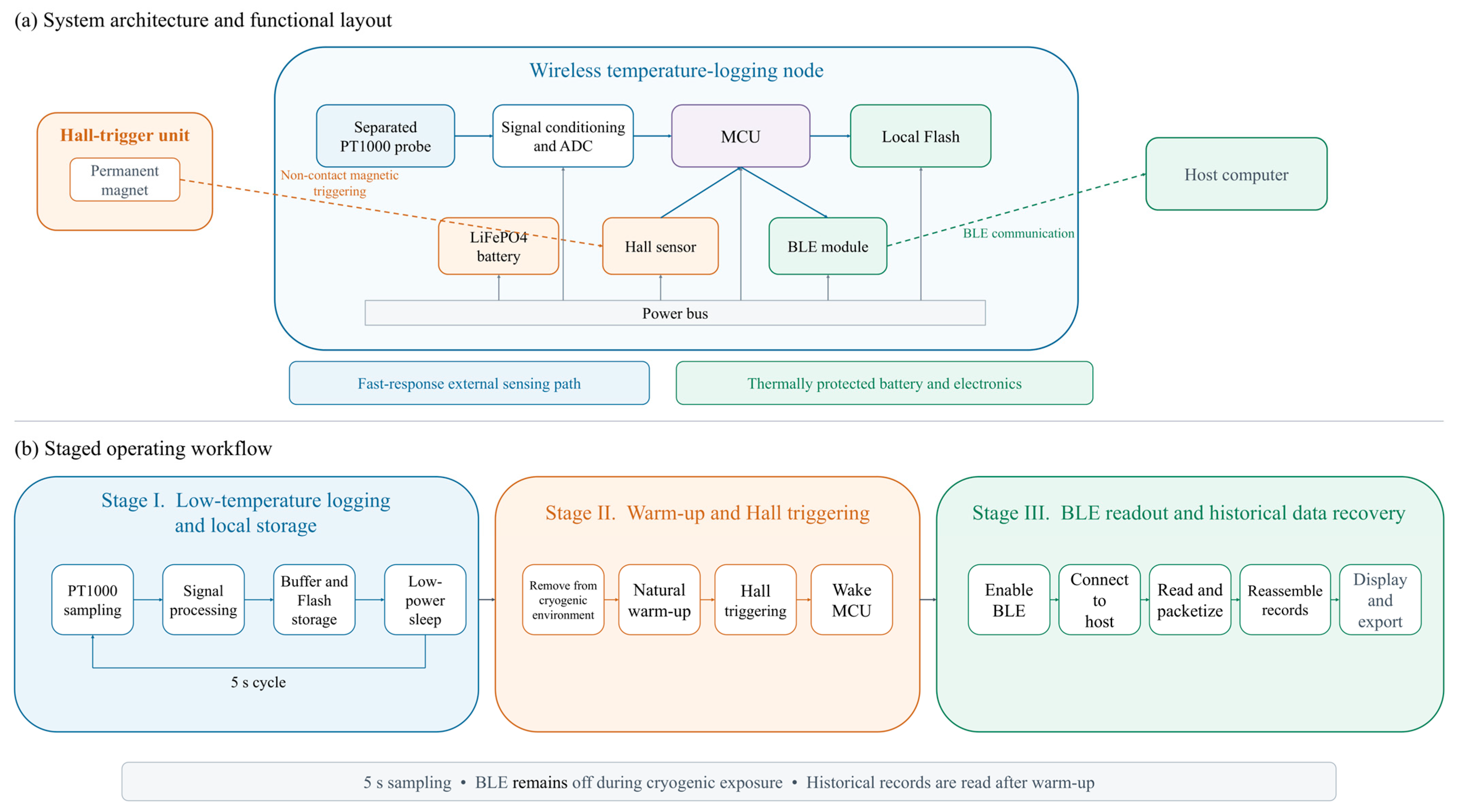
Figure 1. Overall system architecture and staged operating mode: (a) system architecture and functional layout; (b) staged workflow.
Inventions 11 00098 g001
Figure 2. Structure and principal components of the wireless temperature-sensing node: (a) assembled node; (b) principal physical components; (c) exploded view.
Inventions 11 00098 g002
Figure 3. Workflow for low-temperature logging, warm-up triggering, and BLE retrieval of historical data: (a) low-temperature logging and local storage; (b) natural warm-up and Hall-effect triggering; (c) BLE retrieval, record verification, and host-side data processing.
Inventions 11 00098 g003
Figure 4. Geometry, computational mesh, and grid-independence assessment of the wireless temperature-sensing node: (a) node geometry; (b) representative cross-sectional mesh and material domains; (c) predicted temperature histories for coarse (1,355,978 cells), medium (2,552,875 cells), and fine (4,395,554 cells) meshes.
Inventions 11 00098 g004
Figure 5. Structure, cryogenic experiment, and model evaluation of the node with an internal PT1000: (a) standard node and evaluation node; (b) cryogenic exposure apparatus; (c) packaged evaluation node; (d) circuit board; (e) internal component arrangement; (f) experimental, simulated, and ambient temperature histories; (g) absolute temperature error between the aligned experimental and simulated histories. The 0.01 °C rounding component corresponds to u q = 0.0029 °C; no combined system temperature uncertainty is assigned (Section 2.3.2 and Table 2).
Inventions 11 00098 g005
Figure 6. Schematic of measurement levels and locations in the operating biobank. The left panel shows the vertical selection of Layers 1, 8, and 16 within the 16-layer rack: (a) Layer 1 (upper level); (b) Layer 8 (middle level); (c) Layer 16 (lower level). Two planned locations were assigned to each of the inner, middle, and outer rings at every level, giving six locations per level and eighteen locations in total. The schematic represents spatial coverage only and is not drawn to exact angle or scale.
Inventions 11 00098 g006
Figure 7. Engineering performance of the wireless temperature-sensing system: (a) effective cryogenic operating durations of nine nodes, with the dashed line indicating the mean of 44.2 min and the shaded band indicating the combined standard uncertainty of the mean, uc = 0.96 min (k = 1); (b) number of nodes successfully establishing BLE connections during 20–40 min of warm-up; (c) packet-loss rate at different communication distances.
Inventions 11 00098 g007
Figure 8. Measured and numerical reference temperature histories at six locations on Layer 16 (lower level): (a) X09Y16; (b) X20Y16; (c) X32Y16; (d) X35Y16; (e) X46Y16; (f) X55Y16. The temperature traces are shown without a combined standard-uncertainty band because the traceable system-level calibration and complete input uncertainty budget required for such a band were not archived (Section 2.3.2 and Table 2).
Inventions 11 00098 g008
Figure 9. Measured and numerical reference temperature histories at six locations on Layer 8 (middle level): (a) X01Y08; (b) X31Y08; (c) X42Y08; (d) X51Y08; (e) X60Y08; (f) X65Y08. The temperature traces are shown without a combined standard-uncertainty band because the traceable system-level calibration and complete input uncertainty budget required for such a band were not archived (Section 2.3.2 and Table 2).
Inventions 11 00098 g009
Figure 10. Measured and numerical reference temperature histories at six locations on Layer 1 (upper level): (a) X20Y01; (b) X31Y01; (c) X35Y01; (d) X41Y01; (e) X47Y01; (f) X61Y01. The temperature traces are shown without a combined standard-uncertainty band because the traceable system-level calibration and complete input uncertainty budget required for such a band were not archived (Section 2.3.2 and Table 2).
Inventions 11 00098 g010
Table 1. System operating stages.
Operating StageMain TaskLow-Power and Data StrategyTransition Condition
Initialization and deploymentInitialize the clock, acquisition interface, Flash memory, interrupts, and storage pointersBLE disabled; buffer and record starting point establishedDeployment completed and periodic sampling started
Low-temperature acquisition and local storageAcquire the PT1000 signal every 5 s, generate records, and write them to Flash in batchesBrief excitation; batch write and readback verification every 20 records; sleep otherwiseNode removed from the cryogenic environment or acquisition stopped
Warm-up and trigger standbyAllow the node to warm naturally and wait for an external magnetic fieldBLE and nonessential peripherals remain disabled; trigger interface retainedHall-effect sensor detects the external magnetic field
Wireless data retrievalEstablish BLE connection, read Flash sequentially, and transmit historical records in packetsReassemble by sample index and verification fields; disable the radio after retrievalHistorical data retrieval completed
Table 2. Measurement instrumentation, ranges, resolution, and uncertainty status.
Instrument or ChannelModel/ConfigurationMeasurand and Documented RangeResolution or SamplingStandard Uncertainty and Status
Developed PT1000 temperature-logging channelPT1000, two-wire brief constant-current excitation, differential amplification, AD7171BCPZ conversion, IEC 60751 relationshipTemperature; design exposure approximately 25 to −196 °C; model evaluation record −104.26 to 19.06 °C16-bit ADC output; exported increment 0.01 °C; 1 s for model evaluation and 5 s for other testsRounding component u_q = 0.01/√12 = 0.0029 °C. A combined system standard uncertainty was not assigned because a traceable system calibration and complete component-level uncertainty budget were not archived.
Internal time baseArduino Nano 33 BLE Rev2; 32.768 kHz clock retained during exposureElapsed time; 0–3446 s model evaluation record, 38.4–47.2 min operating-duration results, and 5–40 min warm-up observations1 s, 5 s, or 5 min according to the testTimestamp/observation-grid components: 0.29 s (1 s), 1.44 s (5 s), and 1.44 min (5 min), using q/√12. Oscillator calibration uncertainty was not archived. For the nine-node mean operating duration, u_c = 0.96 min (k = 1); see Section 2.3.2.
Straight-line distance setupMarked node-to-host separation; measuring-device record not archivedDistance, 2–16 m2 m test incrementsA combined distance standard uncertainty was not assigned because traceable calibration and repeat-placement data were not archived; the results are therefore an engineering distance screening.
Table 3. System components and implementation details.
Component or FunctionImplementation
Probe structureRemote PT1000 probe with PEEK housing and small-cross-section copper-wire connection
Signal conditioningDifferential amplification and low-pass filtering
MicrocontrollerArduino Nano 33 BLE Rev2 controller
Local storageOn-chip Flash memory with SRAM buffering; batch write every 20 records
BatteryLiFePO4 battery
Hall-effect triggerDRV5033 Hall switch (Texas Instruments Inc., Dallas, TX, USA) and external permanent magnet
Wireless interfaceBluetooth Low Energy, activated after warm-up
Host platformMetrology Works, an in-house-developed host application, for connection management, reception, curve display, and export
Data record fieldsSample index, temperature value, status flag, and 16-bit CRC
Data verification16-bit CRC and post-write readback verification
Low-power strategyBrief excitation; BLE, high-speed oscillator, and nonessential peripherals disabled during cryogenic exposure
Application scopeFinite-duration engineering logging during cryogenic exposure followed by historical record retrieval after warm-up
Table 4. Main material properties used in the node heat-transfer model.
Material or ComponentDensity/(kg·m−3)Thermal Conductivity/(W·m−1·K−1)Specific Heat Capacity/(J·kg−1·K−1)Parameter Category and Description
PTFE21900.2561000C; constant property used in the model; magnitude and temperature dependence checked against cryogenic references
Aerogel82.20.007502.32C; constant property used in the model; the magnitude of 0.007 was checked only against cryogenic-aerogel studies
PEEK13300.29320C; constant property used in the model; magnitude over a limited temperature range checked against cryogenic studies
Copper8978387.6381C; constant property used in the model; actual cryogenic properties vary with temperature
Stainless steel803016.27502.48C; constant property used in the model; actual cryogenic properties vary with temperature
Air1.2250.02421006.43R; constant property at a reference state; not a constant over the full temperature range
Nitrogen gas1.1380.02421038R; constant property at a reference state; not a constant over the full temperature range
Effective circuit-board material16000.21200E; node-level homogenized property; does not represent the separate properties of copper foil, substrate, and solder joints
Effective LiFePO4 battery material36000.8900E; node-level homogenized property; does not represent the separate properties of internal cell constituents
Note: The listed values are constant or node-level effective properties used in the model. Published cryogenic data show that several of these properties vary with temperature [33,34,35,36,37,38,39,40,42,43]. The present calculations did not update the properties with temperature or perform a property-sensitivity analysis; the associated numerical error is therefore not quantified. This assumption is acceptable only for the stated trend-level interpretation and is a principal source of the absolute temperature and response-time discrepancies reported in Section 3.1.
Table 5. Summary of system performance tests.
Test ItemTest Condition or ObjectResult
Effective operating durationNine nodes; 5 s sampling; one complete record per node38.4–47.2 min; mean 44.2 min; median 45.1 min; between-node sample standard deviation 2.87 min; range 8.8 min; coefficient of variation 6.48%; combined standard uncertainty of the mean u_c = 0.96 min (k = 1)
Warm-up reconnectionApproximately 25 °C; eight observation times from 5 to 40 min; Figure 7b shows the 20–40 min results0/9 from 5 to 20 min; 2/9, 5/9, 9/9, and 9/9 at 25, 30, 35, and 40 min, respectively
BLE communicationOne node; indoor environment with limited obstruction and interference; engineering distance screeningNo packet loss observed from 2 to 10 m; packet-loss rates of 2%, 8%, and 10% at 12, 14, and 16 m, respectively
Field deploymentLayers 16, 8, and 1; 6 planned locations per layer; 18 locations in total; sequential testing; 5 s samplingEighteen retrievable measured temperature histories obtained; both measured and corresponding numerical reference curves showed rapid early cooling followed by progressively slower cooling; not used for synchronous full-field reconstruction or metrology-grade error evaluation
Disclaimer/Publisher’s Note: The statements, opinions and data contained in all publications are solely those of the individual author(s) and contributor(s) and not of MDPI and/or the editor(s). MDPI and/or the editor(s) disclaim responsibility for any injury to people or property resulting from any ideas, methods, instructions or products referred to in the content.