Domain Walls with Alternating Magnetic Order in a Model with Dipolar Coupling

Abstract

A model for a one-dimensional chain of elongated nano-scale magnetic islands with dipole interactions is analyzed here for the properties of its static domain walls with site-by-site alternating order. The anisotropic magnetic islands on a nonmagnetic substrate have their longer axes oriented transverse (y-direction) to the chain direction (x-direction), in a transverse applied magnetic field. The islands’ magnetic dipoles ${\mathit{\mu }}_n$ are represented as macrospins of fixed length $\mu$. The nearest neighbor (NN) dipole interactions drive transverse alternating order, allowing for doubly degenerate, uniform, static, y-alternating states, where the dipoles alternately point transverse to the chain direction, as in ${\mathit{\mu }}_n=\pm {(-1)}^n\mu \widehat{\mathit{y}}$. Assuming only NN interactions, the domain walls connecting these two alternating states are found with numerical relaxation simulations and analyzed in a two-sublattice continuum theory. The applied field produces a very slight canting of the dipoles towards the field, maximum in the center of the domain wall. The dipoles on the two sublattices are found to rotate in opposite senses as one scans along the lattice, resulting in a large longitudinal magnetic moment of the domain wall. A much smaller transverse magnetic moment has a topological contribution that depends on whether the chain length is odd or even.

1. Introduction: Multi-Stable Magnetic Island Chains

Nanoscale engineered magnetic arrays such as two-dimensional (2D) spin ices of many geometries [1,2,3] and one-dimensional (1D) chains of thin magnetic islands [4,5,6], existing on nonmagnetic substrates, are systems whose properties might be tunable for desired functions. These systems involve mesoscopic islands whose magnetic dipoles ${\mathit{\mu }}_n$ interact via dipolar interactions that compete with island-shape anisotropies and with an applied field.

1D chains of circular mesoscopic islands were studied in Ref. [7] with the ${\mathrm{Mumax}}^3$ micromagnetics software and found to interact via stray fields equivalent to an XY model modified by short-range “dipole-like” interactions. Other studies in Ref. [8] using ${\mathrm{Mumax}}^3$ led to a nearest neighbor (NN) XY model with variable spin length due to the internal spin textures. A modification to elongated islands would induce shape anisotropy and limit the variation in spin length. Vantaraki et al. [9] made a theoretical and experimental study of stadium-shaped islands pointing transverse to the chain, together with an offset on every other one. The geometry was used to control magnetic order in various phases. Other experimental studies of 2D arrays [10,11] of mesoscopic islands controlled by dipole interactions have found antiferromagnetic-like ordering, presumably controlled by NN dipole-like interactions.

These types of models have uniform metastable states, often existing in symmetry-related pairs, differing only in some quantum number related to that physical symmetry. The symmetry may invert or rotate some spin component(s) to convert one of the paired uniform states into the other, without a change in energy while conserving some component of the total magnetic moment. With the existence of such pairs, domain walls (DWs) exist that connect them over some distance. I avoid referring to them as solitons. This work does not establish any solitary scattering properties for the solutions being found. The analysis is simplest in 1D chains. This work studies a type of 1D DW that connects states with antiferromagnetic-like ordering. I refer to it as alternating order because it is due to dipolar interactions and not antiferromagnetism.

Somewhat like the system studied by Vantaraki et al. [9], here I consider a model [12] of a 1D chain (along x) of islands whose longer axes are oriented transverse (along y) to the chain, without and with a magnetic field applied transversely (along $+y$), and a small thickness along z perpendicular to the substrate. This could be realized by modern techniques, building small chains of slightly elliptical magnetic disks with a regular spacing. Without an applied field, there are three stable or metastable uniform states:

• x-parallel, where the island dipoles all point along $+x$ or $-x$.
• y-parallel (or y-par for short), where the island dipoles all point along $+y$ or $-y$.
• y-alternating (or y-alt for short), where the island dipoles alternate between $+y$ and $-y$ directions.

The two y-alt states are distinguished by either having even/odd dipoles along $+y/-y$ or along $-y/+y$, respectively; see Figure 1. Note that a uniform y-alt configuration minimizes the NN dipolar energy, while uniform y-parallel maximizes it.

Figure 1. A static y-alt² DW centered in a system of 21 islands, with a half-width $h=4$ in lattice constants, embedded between the two possible y-alt states. The red/blue arrows represent the island dipoles on odd/even sublattices, respectively. The sublattices rotate through a 90° angle in opposite senses, while remaining in the $xy$-plane, as one scans along the chain. At the center, the dipoles can point towards $+x$ (as shown) or towards $-x$ by reversing the rotation senses on both sublattices.

When a weak transverse magnetic field is applied, the y-par and y-alt configurations are unchanged, while the dipoles in x-parallel states tilt away from $\pm x$ towards $+y$, resulting in oblique states (dipoles at an oblique angle to $\pm x$). The degeneracy of the two oblique states is obvious, and one is transformed to the other by reversing the x-components of the dipoles. A DW can form between these two oblique states, and the structure and creation energies of those oblique-to-oblique DWs were analyzed in recent work [13]. It was found that an approximate continuum limit for the angles of the dipoles in the $xy$-plane leads to a scalar ${\phi }^4$ equation, which is adequate to describe the oblique-to-oblique DWs.

Numerical simulations [13] also indicated the existence of stable DWs from oblique to y-alt when their energies are close, and between the two degenerate y-alt states. It is difficult to imagine a continuum theory going smoothly from a nearly aligned oblique state to the anti-aligned y-alt state. In contrast, a continuum theory for a configuration connecting the two y-alt states is realizable and developed in this work.

The goal of this report is to develop a continuum theory for the description of the y-alt to y-alt DWs, which are referred to as y-alt² DWs. An example is shown in Figure 1. A significant result is a continuum equilibrium equation for the spin structure of these DWs, and its approximate but exceptionally good solution. That describes the variation of the dipoles from one side of the DW to the other, as well as its net magnetic moment and creation energy. This is done for a limited range of shape anisotropy relative to the NN dipolar coupling. The theory is restricted to finding static DWs with NN dipolar coupling; long-range interactions are likely to shift some results. Numerical simulations of discrete islands in a chain are used to guide and verify the continuum limit and indicate where it fails when the DW becomes too narrow.

In order to verify the static y-alt² DW solutions, I present three methods for their determination.

The first method is numerical relaxation simulations, using the scheme in Ref. [13], where the macrospins are iteratively pointed in the direction of the effective magnetic field that acts on them. This results in zero torque on each spin, together with a local minimum of energy, and hence a stable static DW.

The second method is to find continuum equilibrium equations for the dipole directions by making approximate expansions of the discrete equations of motion for the island dipoles. The continuum theory is developed similar to the two-sublattice approach used for antiferromagnetic chains [14,15,16]. The equilibrium equations so obtained have approximate asymptotic solutions far from the DW center that turn out to work surprisingly well even near the center of the DW.

In a third method, the continuum theory was checked by starting from a continuum expansion of the Hamiltonian and using it for development of the equilibrium equations. This last method confirms those equilibrium equations, but only with careful consideration of up to third-order small terms.

2. The Model for Macrospins Coupled by Dipole Interactions

The islands are assumed to have individual magnetic dipole moments ${\mathit{\mu }}_n=\mu {\mathbf{S}}_n$ of fixed magnitude $\mu$, described by unit length classical Heisenberg-like [17,18] macrospins ${\mathbf{S}}_n$. They are each affected by a transverse uniaxial anisotropy of strength $K_1$ and an easy-plane anisotropy of strength $K_3$, as well as the applied magnetic field $\mathbf{B}=B\widehat{y}$, so that the Hamiltonian involving dipolar interactions among all N dipoles on a chain is

$$\begin{array}{cc}\hfill H={\displaystyle \sum _{n=1}^N}& \{{\displaystyle \sum _{k=1}^R}{\displaystyle \frac{D}{k^3}}\left[{\mathbf{S}}_n·{\mathbf{S}}_{n+k}-3({\mathbf{S}}_n·\widehat{x})({\mathbf{S}}_{n+k}·\widehat{x})\right]\hfill \\ \hfill & -K_1{\left(S_n^y\right)}^2+K_3{\left(S_n^z\right)}^2-\mu B{S}_n^y\}.\hfill \end{array}$$

(1)

The NN dipolar coupling constant is an energy,

$$D\equiv {\displaystyle \frac{{\mu }_0{\mu }^2}{4\pi a^3}},$$

(2)

where ${\mu }_0$ is the permeability of space and a is the lattice constant or center-to-center separation of NN dipoles. The range of the dipole interactions is R. Although dipole interactions are long range, in order to get initial progress, I set $R=1$ and confine the analysis to the NN model. This produces features similar to what happens in the long-range model ($R\to \infty$), but at different coupling parameters. For a finite chain, the interaction sum is cut off when $n+k>N$.

The restriction to NN interactions is unnecessary for the numerical simulations; it is imposed for practical reasons due to the complexity of the continuum analysis for this alternating-order problem. Continuum theory is based on cut-off Taylor expansions and the assumption of slow spatial variations over short distances (a few neighbors). The process is not well-defined if neighbors at long range are to be considered because Taylor expansions only work at short range. Even so, second, fourth, sixth, etc. nearest neighbor dipole interactions in a uniform alternating state will involve parallel dipoles transverse to the chain, with positive energy contributions. The third, fifth, seventh, etc. nearest neighbor dipole interactions will involve antiparallel transverse dipoles and smaller negative energy contributions. The net result is an increase in the energy of y-alt states. This appears to increase the anisotropy strength $K_1$ relative to D that is required for stable y-alt² DWs. However, the study here only compares the NN numerical results with the continuum theory for the NN model.

For classical spin mechanics, a magnetic dipole is related to its angular momentum by ${\mathit{\mu }}_n=\gamma {\mathbf{L}}_n=\mu {\mathbf{S}}_n$, where $\gamma$ is a gyromagnetic ratio. With unit magnitude ${\mathbf{S}}_n$ being dimensionless, the angular momentum of a dipole is $\mu /\gamma$. The rate of change of ${\mathbf{L}}_n$ is equal to the net torque on that dipole, which gives the basic dynamic equation,

$${\displaystyle \frac{1}{\gamma }}{\displaystyle \frac{d{\mathit{\mu }}_n}{dt}}={\mathit{\mu }}_n\times {\mathbf{B}}_n={\mathit{\mu }}_n\times \left(-{\displaystyle \frac{\partial H}{\partial {\mathit{\mu }}_n}}\right).$$

(3)

${\mathbf{B}}_n$ is the net effective magnetic field acting on a dipole, caused by dipolar and anisotropic effects as well as the applied magnetic field.

The classical equations of motion can be developed in terms of the Cartesian spin components; however, it is more advantageous to use planar spherical angular coordinates, representing the macrospin components as

$$\begin{array}{cc}\hfill {\mathbf{S}}_n& =(S_n^x,S_n^y,S_n^z)\hfill \\ \hfill & =(cos{\theta }_{n}cos{\varphi }_n,cos{\theta }_{n}sin{\varphi }_n,sin{\theta }_n).\hfill \end{array}$$

(4)

For one dipole, the angle ${\varphi }_n$ can be viewed as a coordinate, and $(\mu /\gamma )S_n^z=(\mu /\gamma )sin{\theta }_n$ is the momentum conjugate to that coordinate. Then the vector dynamic equation is equivalent to Hamiltonian dynamic equations for the angles,

$$\begin{array}{c}\hfill {\displaystyle \frac{d}{dt}}{\varphi }_n={\displaystyle \frac{\partial H}{\partial \left(\frac{\mu }{\gamma }sin{\theta }_n\right)}},{\displaystyle \frac{d}{dt}}\left(\frac{\mu }{\gamma }sin{\theta }_n\right)=-{\displaystyle \frac{\partial H}{\partial {\varphi }_n}}.\end{array}$$

(5)

The system Hamiltonian limited to NN interactions is expressed using angular coordinates as

$$\begin{array}{cc}\hfill H& ={\displaystyle \sum _{n=1}^N}\{D[sin{\theta }_{n}sin{\theta }_{n+1}+cos{\theta }_{n}cos{\theta }_{n+1}\hfill \\ \hfill & \times (-2cos{\varphi }_{n}cos{\varphi }_{n+1}+sin{\varphi }_{n}sin{\varphi }_{n+1})]\hfill \\ \hfill & -K_1{cos}^2{\theta }_n{sin}^2{\varphi }_n+K_3{sin}^2{\theta }_n-\mu Bcos{\theta }_{n}sin{\varphi }_n\}.\hfill \end{array}$$

(6)

Then the discrete Hamiltonian dynamic equations for the in-plane angles are

$$\begin{array}{cc}\hfill {\displaystyle \frac{\mu }{\gamma }}& {\displaystyle \frac{d}{dt}}{\varphi }_n={\displaystyle \frac{\partial H}{\partial sin{\theta }_n}}=D[sin{\theta }_{n-1}+sin{\theta }_{n+1}\hfill \\ \hfill & +2tan{\theta }_{n}cos{\varphi }_n(cos{\theta }_{n-1}cos{\varphi }_{n-1}+cos{\theta }_{n+1}cos{\varphi }_{n+1})\hfill \\ \hfill & -tan{\theta }_{n}sin{\varphi }_n(cos{\theta }_{n-1}sin{\varphi }_{n-1}+cos{\theta }_{n+1}sin{\varphi }_{n+1})]\hfill \\ \hfill & +2K_{1}sin{\theta }_n{sin}^2{\varphi }_n+2K_{3}sin{\theta }_n+\mu Btan{\theta }_{n}sin{\varphi }_n.\hfill \end{array}$$

(7)

For the out-of-plane angle, there results

$$\begin{array}{cc}\hfill {\displaystyle \frac{\mu }{\gamma }}& {\displaystyle \frac{d}{dt}}{\theta }_n=-sec{\theta }_n{\displaystyle \frac{\partial H}{\partial {\varphi }_n}}\hfill \\ \hfill & =-D[2sin{\varphi }_n(cos{\theta }_{n-1}cos{\varphi }_{n-1}+cos{\theta }_{n+1}cos{\varphi }_{n+1})\hfill \\ \hfill & +cos{\varphi }_n(cos{\theta }_{n-1}sin{\varphi }_{n-1}+cos{\theta }_{n+1}sin{\varphi }_{n+1})]\hfill \\ \hfill & +2K_{1}cos{\theta }_{n}sin{\varphi }_{n}cos{\varphi }_n+\mu Bcos{\varphi }_n.\hfill \end{array}$$

(8)

One can note that the dipolar terms in both dynamic equations contain NN angles surrounding the central site n. For simplicity, define dimensionless anisotropies and applied field,

$$k_1\equiv {\displaystyle \frac{K_1}{D}},k_3\equiv {\displaystyle \frac{K_3}{D}},b\equiv {\displaystyle \frac{\mu B}{D}}.$$

(9)

Energies will be found in units of D.

3. Alternating DW Structures Found by Numerical Simulations

It was noticed in previous work [13] that DWs connecting the two y-alt uniform states exist, and that the spin structure within the DWs themselves has a site-by-site alternating component, similar to what occurs in solitons in antiferromagnetic (AFM) chains [14,15]. These DWs connect the even y-alt state (${\varphi }_n=+/-90°$ on even/odd sites) to the odd y-alt state (${\varphi }_n=+/-90°$ on odd/even sites). The y-alt states exist over a range of model parameters, especially constrained by $k_1>1$, and a limited value of $\left|b\right|$ that depends on $k_1$. The point $k_1=1$ is not included. Physically, at that point, the two y-alt states could exist, but with infinite width.

The structures of these DWs with alternating order were not analyzed in Ref. [13]. In this new work, their width, energy, and magnetic moments are related to the anisotropy parameters and applied field. To reach that goal, numerical simulations of the structures have been used in combination with the development of a new continuum theory for this type of DW in the presence of localized dipolar interactions. The numerical simulations easily determine the static DW structures by an iteration procedure, and those results are compared with approximate predictions found in a somewhat tedious continuum analysis. The comparison helps to to show how the continuum theory breaks down when the DW width becomes too narrow.

For the simulations, $k_3$ is set to zero, although thin islands would have values of $k_3$ greater than $k_1$ due to the higher demagnetization factor in the shorter dimension. This study concerns the static structure, however, and Equation (7) is solved by ${\theta }_n=0$ for all sites when static equilibrium is reached, for any value of $k_3$. Further, the static structure is ultimately determined by Equation (8), which does not contain $k_3$. The static structure is independent of the choice of non-negative $k_3$.

The simulations go as follows [13]. First, an initial configuration of the dipoles is defined by setting the left half of the system in the even y-alt state, abruptly connected to the right half of the system in the odd y-alt state. To avoid highly symmetric anomalies, the macrospin components were changed with a small randomness of amplitude ${10}^{-4}$, followed by rescaling to unit length. At each site, there is a net effective field ${\mathbf{B}}_n$ as defined in Equation (3), produced by its neighbors, the anisotropies, and the applied field. At equilibrium, each dipole would be aligned with that effective field, resulting in zero torque on it. Therefore, to move toward equilibrium, each macrospin is then pointed in the direction of its ${\mathbf{B}}_n$ by

$${\mathbf{S}}_n={\displaystyle \frac{{\mathbf{B}}_n}{\left|{\mathbf{B}}_n\right|}}.$$

(10)

One step corresponds to updating each site in the system once. The process is iterated and moves the system to lower total energy. The energy tends to converge to a constant value faster than the spin structure. To decide when to stop the iteration, an average spin change per site was calculated for each step,

$$\delta S\equiv {\displaystyle \frac{1}{N}}\sum _n\left(|\Delta S_n^x|+|\Delta S_n^y|+|\Delta S_n^z|\right),$$

(11)

where $\Delta {\mathbf{S}}_n$ is the one-step change in a macrospin. The iteration is stopped when $\delta S<{10}^{-9}$. The number of iterations needed can be a few hundred if the state is very stable or as high as 5000 or more if the state is only moderately stable, which can occur if the DW is tending to move out of the system. The procedure can also include a weak Lifshitz–Gilbert damping but it generally makes no difference in the final state and little difference in the convergence rate.

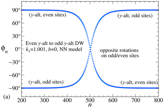
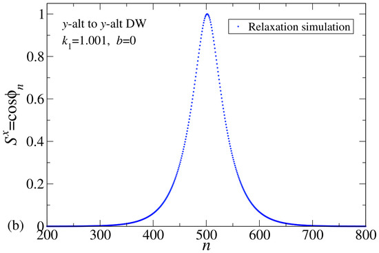
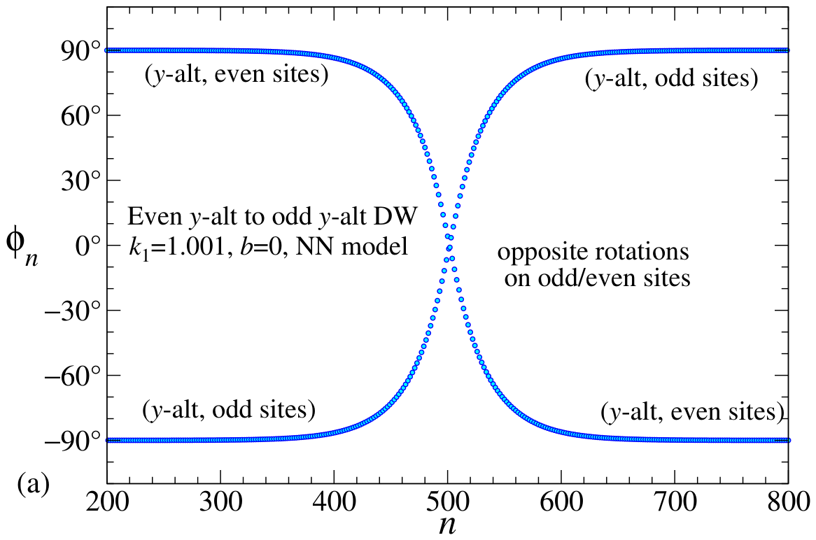
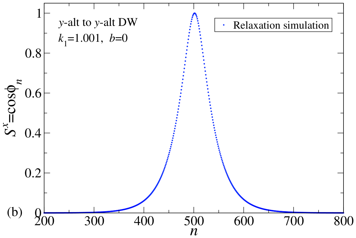
For $k_1=1.001$ and $k_3=b=0$, a y-alt² DW is displayed in Figure 2, where the even y-alt state is on the left side of the system, connecting to the odd y-alt state on the right side of the system. Figure 2a shows the in-plane angles ${\varphi }_n$ on the discrete sites; the out-of-plane angles ${\theta }_n$ are zero for any static configuration of the model. It is significant that the dipoles make opposing rotations on the two sublattices as one moves along the chain. This is important when it comes to constructing a continuum limit for this problem. In Figure 2b, the macrospin components parallel to the chain direction are shown. It is notable that there is no distinction between the x-components on the two sublattices (for $b=0$ only). This type of DW is found only for $k_1>1$.

Figure 2. A y-alt to y-alt DW in the NN model from numerical relaxation simulations at $k_1=1.001$, $b=0$. (a) The in-plane angles, identified by odd/even sublattices. (b) The x-components of the macrospins. The view is zoomed in on the $N=1000$ system. The half-width $h=37a$ was estimated from the tangent line in ${\varphi }_{n=\mathrm{odd}}$ at the DW center. For $k_1$ farther above unity, the DW width is narrower.

4. Continuum Equations Derived from the Discrete Lattice Equations

A continuum description of the DWs is helpful for predicting how their structures depend on the physical parameters $k_1,k_3$, and b. The intention is to find the continuum differential equations for describing the dipoles along coordinate $x=na$. To do this, the alternating structure must be accounted for. We observe that the dipole angles start at $\pm 90°$ on the two sublattices (even vs. odd sites) on one side of the DW. They reduce in magnitude until reaching zero at the DW center, and then emerge to $\mp 90°$ on the other side (Figure 1). They rotate in opposite senses as one passes through the DW along the chain (Figure 2a). Alternatively, they could have passed through 180° at the DW center, i.e., forming a DW with the opposite helicity. The dipoles on the two sublattices maintain the same x-components through the DW, as in Figure 2b. The two sublattices’ dipoles are parallel at the DW center, even for $b\ne 0$.

These facts are incorporated by mapping the discrete site angles ${\varphi }_n,{\theta }_n,$ into continuum large angles $\mathrm{\Phi }\left(x\right)$ and $\mathrm{\Theta }\left(x\right)$ and small angles $\phi \left(x\right)$ and $\vartheta \left(x\right)$ according to the opposing rotations assumption,

$$\begin{array}{cc}\hfill {\varphi }_n& \to \left\{\begin{array}{cc}+\mathrm{\Phi }\left(x\right)+\phi \left(x\right),\hfill & n=\mathrm{even}.\hfill \\ -\mathrm{\Phi }\left(x\right)+\phi \left(x\right),\hfill & n=\mathrm{odd}.\hfill \end{array}\right.\hfill \\ \hfill {\theta }_n& \to \left\{\begin{array}{cc}+\mathrm{\Theta }\left(x\right)+\vartheta \left(x\right),\hfill & n=\mathrm{even}.\hfill \\ -\mathrm{\Theta }\left(x\right)+\vartheta \left(x\right),\hfill & n=\mathrm{odd}.\hfill \end{array}\right.\hfill \end{array}$$

(12)

One might consider the large angles as alternating or antiferromagnetic components and the small angles as aligned or ferromagnetic components. The small angles are generally considered one order smaller than the large angles. Later, $\phi$ and $\vartheta$ are shown to increase with the applied field b. At $b=0$, the small angles are zero. For opposing rotations at $b=0$, the two sublattices have the same $S^x$ but opposite $S^y$ and $S^z$. That is in contrast to the opposite directions assumption generally used to describe DWs in 1D antiferromagnets, where the two sublattices are approximately antiparallel in Mikeska’s assumption [14,15,19]. However, 1D antiferromagnets apparently also support solitons with opposing rotations on the sublattices, if one looks carefully enough [19,20].

4.1. In-Plane Dynamic Equations

Now the discrete Equation (7) are expanded into their equivalent continuum form, under the opposing rotations assumption. Suppose a site n is even. In addition to Equation (12), we have for its first neighbors, both on the odd sublattice,

$$\begin{array}{cc}\hfill {\varphi }_{n+1}& =-\mathrm{\Phi }(x+a)+\phi (x+a),\hfill \\ \hfill {\varphi }_{n-1}& =-\mathrm{\Phi }(x-a)+\phi (x-a),n=\mathrm{even}.\hfill \end{array}$$

(13)

Similar expressions apply to the out-of-plane angles. Then use Taylor expansions, keeping up to quadratic terms in the small angles and in space derivatives of the large angles. Ignore spatial variations of the small angles.

$$\begin{array}{cc}\hfill \mathrm{\Phi }(x+a)& \approx \mathrm{\Phi }\left(x\right)+a{\mathrm{\Phi }}_x\left(x\right)+\frac{1}{2}{a}^2{\mathrm{\Phi }}_{xx}\left(x\right),\hfill \\ \hfill \mathrm{\Theta }(x+a)& \approx \mathrm{\Theta }\left(x\right)+a{\mathrm{\Theta }}_x\left(x\right)+\frac{1}{2}{a}^2{\mathrm{\Theta }}_{xx}\left(x\right).\hfill \end{array}$$

(14)

From here, I will write $\mathrm{\Phi }$, $\mathrm{\Theta }$ to indicate $\mathrm{\Phi }\left(x\right)$, $\mathrm{\Theta }\left(x\right)$, and the same for the derivatives. The small angles do not require expansions. In addition, one needs expansions of various trigonometric functions, such as

$$\begin{array}{cc}\hfill cos{\varphi }_{n+1}& \approx cos[-\mathrm{\Phi }(x+a)+\phi (x+a\left)\right]\hfill \\ \hfill & \approx cos[\phi -\mathrm{\Phi }-a{\mathrm{\Phi }}_x-\frac{1}{2}{a}^2{\mathrm{\Phi }}_{xx}]\hfill \\ \hfill & \approx cos\mathrm{\Phi }[1-\frac{1}{2}\left({\phi }^2+a^2{\mathrm{\Phi }}_x^2-2a\phi {\mathrm{\Phi }}_x\right)]\hfill \\ \hfill & +sin\mathrm{\Phi }[\phi -a{\mathrm{\Phi }}_x-\frac{1}{2}{a}^2{\mathrm{\Phi }}_{xx}].\hfill \end{array}$$

(15)

There is a corresponding expansion,

$$\begin{array}{cc}\hfill sin{\varphi }_{n+1}& \to sin[-\mathrm{\Phi }(x+a)+\phi (x+a\left)\right]\hfill \\ \hfill & \approx sin[\phi -\mathrm{\Phi }-a{\mathrm{\Phi }}_x-\frac{1}{2}{a}^2{\mathrm{\Phi }}_{xx}]\hfill \\ \hfill & \approx -sin\mathrm{\Phi }[1-\frac{1}{2}\left({\phi }^2+a^2{\mathrm{\Phi }}_x^2-2a\phi {\mathrm{\Phi }}_x\right)]\hfill \\ \hfill & +cos\mathrm{\Phi }[\phi -a{\mathrm{\Phi }}_x-\frac{1}{2}{a}^2{\mathrm{\Phi }}_{xx}].\hfill \end{array}$$

(16)

There are similar expansions for the same functions of ${\theta }_{n+1}$. Further, these expressions give the values at the opposite near neighbor $n-1$ by changing $a\to -a$. Then, summing over left and right nearest neighbors, the terms linear in a cancel out, and one gets twice the even terms in a, such as the first dipole interaction term in Equation (7),

$$\begin{array}{cc}\hfill d_1& \equiv sin{\theta }_{n-1}+sin{\theta }_{n+1}\hfill \\ \hfill \approx & -sin\mathrm{\Theta }(2-{\vartheta }^2-a^2{\mathrm{\Theta }}_x^2)+cos\mathrm{\Theta }(2\vartheta -a^2{\mathrm{\Theta }}_{xx}).\hfill \end{array}$$

(17)

There are two more dipole interaction contributions $d_2$ and $d_3$, in the second and third lines of Equation (7), which are expanded in Appendix A. The expansions of the anisotropy and field terms are straightforward and also shown in Appendix A. I define a dimensionless time variable,

$$\tau \equiv {\displaystyle \frac{\gamma D}{\mu }}t,$$

(18)

and use dot to indicate derivative with respect to $\tau$. From the opposing rotations assumption (Equation (12)), the discrete dynamic equations found for even-n sites and for odd-n sites are related to the desired continuum equations by the following:

$$\begin{array}{cc}\hfill \dot{\mathrm{\Phi }}& =\frac{1}{2}({\dot{\varphi }}_{\mathrm{evn}}-{\dot{\varphi }}_{\mathrm{odd}}),\hfill \\ \hfill \dot{\phi }& =\frac{1}{2}({\dot{\varphi }}_{\mathrm{evn}}+{\dot{\varphi }}_{\mathrm{odd}}).\hfill \end{array}$$

(19)

${\dot{\varphi }}_{\mathrm{evn}}$ and ${\dot{\varphi }}_{\mathrm{odd}}$ are defined by Equation (7) expanded in the continuum angles for even and odd n, respectively, which is done in Appendix A. From here, position x will be measured in units of a, equivalent to setting $a=1$ in the equations. Then, the net continuum equation for the large in-plane angle, expanded to quadratic order of small terms, is,

$$\begin{array}{cc}\hfill \dot{\mathrm{\Phi }}& \approx sin\mathrm{\Theta }{cos}^2\mathrm{\Phi }(2-{\mathrm{\Theta }}_x^2)-(1+{cos}^2\mathrm{\Phi })sin\mathrm{\Theta }\left({\mathrm{\Phi }}_x^2\right)\hfill \\ \hfill & +tan\mathrm{\Theta }sin\mathrm{\Theta }sin2\mathrm{\Phi }\left({\mathrm{\Theta }}_x{\mathrm{\Phi }}_x\right)-sin\mathrm{\Theta }sin2\mathrm{\Phi }\left(\frac{1}{2}{\mathrm{\Phi }}_{xx}\right)\hfill \\ \hfill & -sec\mathrm{\Theta }(1+{sin}^2\mathrm{\Theta }{cos}^2\mathrm{\Phi }){\mathrm{\Theta }}_{xx}-6{\phi }^{2}sin\mathrm{\Theta }\hfill \\ \hfill & +4{\vartheta }^{2}sin\mathrm{\Theta }\left[{sec}^2\mathrm{\Theta }+\left({sec}^2\mathrm{\Theta }-\frac{1}{4}\right){cos}^2\mathrm{\Phi }\right]\hfill \\ \hfill & +2k_1[\left(1-\frac{1}{2}{\vartheta }^2\right)sin\mathrm{\Theta }{sin}^2\mathrm{\Phi }+{\phi }^{2}sin\mathrm{\Theta }cos2\mathrm{\Phi }\hfill \\ \hfill & +\phi \vartheta cos\mathrm{\Theta }sin2\mathrm{\Phi }]+2k_3\left(1-\frac{1}{2}{\vartheta }^2\right)sin\mathrm{\Theta }\hfill \\ \hfill & +b\left(\vartheta {sec}^2\mathrm{\Theta }sin\mathrm{\Phi }+\phi tan\mathrm{\Theta }cos\mathrm{\Phi }\right).\hfill \end{array}$$

(20)

The first four lines are the dipolar terms. The net continuum equation for the small in-plane angle, also to quadratic order, is,

$$\begin{array}{cc}\hfill \dot{\phi }& \approx 2\vartheta sec\mathrm{\Theta }\left\{2+\left(1+{sin}^2\mathrm{\Theta }\right){cos}^2\mathrm{\Phi }\right\}\hfill \\ \hfill & +2k_1\left(\vartheta cos\mathrm{\Theta }{sin}^2\mathrm{\Phi }+\phi sin\mathrm{\Theta }sin2\mathrm{\Phi }\right)+2k_3\vartheta cos\mathrm{\Theta }\hfill \\ \hfill & +b[\left(1-\frac{1}{2}{\phi }^2+{\vartheta }^2{sec}^2\mathrm{\Theta }\right)tan\mathrm{\Theta }sin\mathrm{\Phi }\hfill \\ \hfill & +\vartheta \phi {sec}^2\mathrm{\Theta }cos\mathrm{\Phi }].\hfill \end{array}$$

(21)

4.2. Out-of-Plane Dynamic Equations

A similar expansion is carried out in Appendix A for the out-of-plane continuum large and small angles. The opposing rotations assumption (12) gives the relation connecting them to the discrete angles on even-n and odd-n sites,

$$\begin{array}{cc}\hfill \dot{\mathrm{\Theta }}& =\frac{1}{2}({\dot{\theta }}_{\mathrm{evn}}-{\dot{\theta }}_{\mathrm{odd}}),\hfill \\ \hfill \dot{\vartheta }& =\frac{1}{2}({\dot{\theta }}_{\mathrm{evn}}+{\dot{\theta }}_{\mathrm{odd}}).\hfill \end{array}$$

(22)

where ${\dot{\theta }}_{\mathrm{evn}}$ and ${\dot{\theta }}_{\mathrm{odd}}$ are defined by Equation (8) expanded in the continuum angles for even and odd n, respectively. The result for the large out-of-plane angle, to quadratic order terms, is,

$$\begin{array}{cc}\hfill \dot{\mathrm{\Theta }}& \approx cos\mathrm{\Theta }[-sin2\mathrm{\Phi }+{\mathrm{\Phi }}_{xx}(2{sin}^2\mathrm{\Phi }+{cos}^2\mathrm{\Phi })\hfill \\ \hfill & +sin\mathrm{\Phi }cos\mathrm{\Phi }\{{\vartheta }^2+{\mathrm{\Theta }}_x^2+{\mathrm{\Phi }}_x^2\}]+sin\mathrm{\Theta }[{\mathrm{\Theta }}_{xx}sin\mathrm{\Phi }cos\mathrm{\Phi }\hfill \\ \hfill & -6\vartheta \phi -2{\mathrm{\Theta }}_x{\mathrm{\Phi }}_x(2{sin}^2\mathrm{\Phi }+{cos}^2\mathrm{\Phi })]\hfill \\ \hfill & +k_1\{(1-2{\phi }^2-\frac{1}{2}{\vartheta }^2)cos\mathrm{\Theta }sin2\mathrm{\Phi }\hfill \\ \hfill & -2\vartheta \phi sin\mathrm{\Theta }cos2\mathrm{\Phi }\}-b\phi sin\mathrm{\Phi }.\hfill \end{array}$$

(23)

For the small out-of-plane angle, there results

$$\begin{array}{cc}\hfill \dot{\vartheta }\approx & -(6\phi cos\mathrm{\Theta }+\vartheta sin\mathrm{\Theta }sin2\mathrm{\Phi })\hfill \\ \hfill & +k_1(2\phi cos\mathrm{\Theta }cos2\mathrm{\Phi }-\vartheta sin\mathrm{\Theta }sin2\mathrm{\Phi })\hfill \\ \hfill & +b\left(1-\frac{1}{2}{\phi }^2\right)cos\mathrm{\Phi }.\hfill \end{array}$$

(24)

All four dynamic equations have considerable complexity, and up to now, I have not found dynamic DW solutions. The analysis here focuses on static solutions, for which the out-of-plane angles become zero.

5. Continuum Equations via a Hamiltonian Density

With the continuum dynamic equations found by expansion of the discrete ones being complicated, a Hamiltonian approach was also used for verification. For the NN model with range $R=1$, the discrete Hamiltonian (1) in planar spherical coordinates is

$$\begin{array}{cc}\hfill H& =\sum _n\{D[sin{\theta }_{n}sin{\theta }_{n+1}+cos{\theta }_{n}cos{\theta }_{n+1}\times \hfill \\ \hfill & (-2cos{\varphi }_{n}cos{\varphi }_{n+1}+sin{\varphi }_{n}sin{\varphi }_{n+1})]\hfill \\ \hfill & -K_1{cos}^2{\theta }_n{sin}^2{\varphi }_n+K_3{sin}^2{\theta }_n-\mu Bcos{\theta }_{n}sin{\varphi }_n\}.\hfill \end{array}$$

(25)

In the continuum theory, the Hamiltonian density $\mathcal{H}$ is effectively the energy per island, defined implicitly by

$$H=\int dx\mathcal{H}.$$

(26)

Using the opposing rotations assumption (12), $\mathcal{H}$ can be expressed in terms of the large and small continuum angles. The result must be expanded to the minimum order necessary to recover the continuum dynamic equations up to second-order small terms. For that to work out, it is necessary to get $\mathcal{H}$ while including up to third-order small terms because the dynamic equations are obtained by its derivatives with respect to the angular coordinates and their gradients.

The continuum expansion of $\mathcal{H}$ for opposing rotations, found in Appendix B, is

$$\begin{array}{cc}\hfill {\displaystyle \frac{\mathcal{H}}{D}}& =-1+{cos}^2\mathrm{\Theta }\left[-{cos}^2\mathrm{\Phi }+(1-\frac{1}{2}{cos}^2\mathrm{\Phi }){\mathrm{\Phi }}_x^2+3{\phi }^2\right]\hfill \\ \hfill & +(1+{sin}^2\mathrm{\Theta }{cos}^2\mathrm{\Phi })\frac{1}{2}{\mathrm{\Theta }}_x^2+\frac{1}{4}(sin2\mathrm{\Theta }sin2\mathrm{\Phi }){\mathrm{\Theta }}_x{\mathrm{\Phi }}_x\hfill \\ \hfill & +(2+{cos}^2\mathrm{\Phi }){\vartheta }^2\hfill \\ \hfill & -k_1[{cos}^2\mathrm{\Theta }({sin}^2\mathrm{\Phi }+{\phi }^{2}cos2\mathrm{\Phi })-{\vartheta }^{2}cos2\mathrm{\Theta }{sin}^2\mathrm{\Phi }\hfill \\ \hfill & -\vartheta \phi sin2\mathrm{\Theta }sin2\mathrm{\Phi }]+k_3\left({sin}^2\mathrm{\Theta }+{\vartheta }^{2}cos2\mathrm{\Theta }\right)\hfill \\ \hfill & -b[-\left(\vartheta -\frac{1}{6}{\vartheta }^3-\frac{1}{2}\vartheta {\phi }^2\right)sin\mathrm{\Theta }sin\mathrm{\Phi }\hfill \\ \hfill & +\left(\phi -\frac{1}{6}{\phi }^3-\frac{1}{2}\phi {\vartheta }^2\right)cos\mathrm{\Theta }cos\mathrm{\Phi }].\hfill \end{array}$$

(27)

The dipolar terms in the first three lines would be different if instead opposite directions was assumed. The anisotropy and field terms do not depend on the assumption. Only the Oersted energy term has third-order small terms. Symmetry eliminates them from the dipolar and anisotropy parts.

For the continuum dynamics, the Hamiltonian Equation (5) need to be expressed in terms of the angles $\mathrm{\Phi },\phi ,\mathrm{\Theta }$, and $\vartheta$. The transformation is demonstrated in Appendix B. For the in-plane angles, the dynamics is

$$\begin{array}{cc}\hfill \dot{\mathrm{\Phi }}& =sec\mathrm{\Theta }\left\{\left[1+{\vartheta }^2\left({tan}^2\mathrm{\Theta }+\frac{1}{2}\right)\right]{\displaystyle \frac{\partial H}{\partial \mathrm{\Theta }}}+\vartheta tan\mathrm{\Theta }{\displaystyle \frac{\partial H}{\partial \vartheta }}\right\},\hfill \\ \hfill \dot{\phi }& =sec\mathrm{\Theta }\left\{\vartheta tan\mathrm{\Theta }{\displaystyle \frac{\partial H}{\partial \mathrm{\Theta }}}+\left[1+{\vartheta }^2\left({tan}^2\mathrm{\Theta }+\frac{1}{2}\right)\right]{\displaystyle \frac{\partial H}{\partial \vartheta }}\right\}.\hfill \end{array}$$

(28)

The partial derivatives are interpreted as functional derivatives of the Hamiltonian, i.e.,

$${\displaystyle \frac{\partial H}{\partial \mathrm{\Theta }}}⟶{\displaystyle \frac{\delta \mathcal{H}}{\delta \mathrm{\Theta }}}={\displaystyle \frac{\partial \mathcal{H}}{\partial \mathrm{\Theta }}}-{\displaystyle \frac{d}{dx}}\left({\displaystyle \frac{\partial \mathcal{H}}{\partial {\mathrm{\Theta }}_x}}\right).$$

(29)

Similar equations apply to the out-of-plane dynamics,

$$\begin{array}{cc}\hfill \dot{\mathrm{\Theta }}& =-sec\mathrm{\Theta }\left\{\left[1+{\vartheta }^2\left({tan}^2\mathrm{\Theta }+\frac{1}{2}\right)\right]{\displaystyle \frac{\partial H}{\partial \mathrm{\Phi }}}+\vartheta tan\mathrm{\Theta }{\displaystyle \frac{\partial H}{\partial \phi }}\right\}.\hfill \\ \hfill \dot{\vartheta }& =-sec\mathrm{\Theta }\left\{\vartheta tan\mathrm{\Theta }{\displaystyle \frac{\partial H}{\partial \mathrm{\Phi }}}+\left[1+{\vartheta }^2\left({tan}^2\mathrm{\Theta }+\frac{1}{2}\right)\right]{\displaystyle \frac{\partial H}{\partial \phi }}\right\},\hfill \end{array}$$

(30)

Equations of comparable form were developed for the problem of solitons in AFM chains [14,15]. When Equations (28) and (30) are applied to the Hamiltonian density (27), the dynamic equations up to second-order small terms agree with those found in Section 4, which were obtained by expansion of the discrete equations of motion.

6. Continuum Equations for Static Equilibrium

If all ${\dot{\varphi }}_n=0$, the discrete dynamic Equation (7) is satisfied by putting all ${\theta }_n=0$. Thus, static solutions take a planar form, which was also obtained in the numerical relaxation simulations.

For statics, the continuum out-of-plane angles $\mathrm{\Theta },\vartheta$ both become zero because ${\theta }_n=0$ for all even and odd sites. This reduces the in-plane dynamic Equations (20) and (21) identically to $\dot{\mathrm{\Phi }}=0$ and $\dot{\phi }=0$. The out-of-plane dynamic Equations (23) and (24) control the statics. In this planar case, the equilibrium equations are

$$\begin{array}{cc}\hfill \dot{\mathrm{\Theta }}\approx & -\left(1-\frac{1}{2}{\mathrm{\Phi }}_x^2\right)sin2\mathrm{\Phi }+{\mathrm{\Phi }}_{xx}(2{sin}^2\mathrm{\Phi }+{cos}^2\mathrm{\Phi })\hfill \\ \hfill & +k_1(1-2{\phi }^2)sin2\mathrm{\Phi }-b\phi sin\mathrm{\Phi }=0.\hfill \end{array}$$

(31)

$$\begin{array}{cc}\hfill \dot{\vartheta }\approx & -6\phi +2k_1\phi cos2\mathrm{\Phi }+b\left(1-\frac{1}{2}{\phi }^2\right)cos\mathrm{\Phi }=0.\hfill \end{array}$$

(32)

The latter gives $\phi$ to linear order in the field b,

$$\phi \approx {\displaystyle \frac{bcos\mathrm{\Phi }}{2(3-k_{1}cos2\mathrm{\Phi })}},$$

(33)

and this eliminates $\phi$ from (31), which becomes the equilibrium equation in the opposing rotations scenario,

$$\begin{array}{cc}\hfill \dot{\mathrm{\Theta }}=& (k_1-1+\frac{1}{2}{\mathrm{\Phi }}_x^2)sin2\mathrm{\Phi }+(2-{cos}^2\mathrm{\Phi }){\mathrm{\Phi }}_{xx}\hfill \\ \hfill & -{\displaystyle \frac{b^2}{4}}{\displaystyle \frac{(3+k_1)sin2\mathrm{\Phi }}{{(3-k_{1}cos2\mathrm{\Phi })}^2}}=0.\hfill \end{array}$$

(34)

This equation is the basis for finding static y-alt² DW solutions in the continuum theory. Approximate but very good solutions for the continuum in-plane structure are described next.

7. Continuum Static DWs with $\mathit{B}=\mathbf{0}$

The field b breaks symmetry between the sublattices. Initially, consider $b=0=\phi$, and refer to the DW in Figure 2 found numerically. The in-plane angle ${\varphi }_n$ for the even-n sublattice is $\mathrm{\Phi }$, which has a large slope at the DW center, but zero slope as $x\to \pm \infty$ (supposing an infinitely long system). The almost constant slope near the center suggests a possible power-series analysis there; however, I did not find that fruitful. Instead, an asymptotic analysis for $x\to \pm \infty$ works well, where Equation (34) exhibits exponential behavior.

For the asymptotic analytics, I consider a DW centered at the origin, with an approximate half-width h. The angle $\mathrm{\Phi }$ can take asymptotic values $\mathrm{\Phi }(-\infty )=\pm {\displaystyle \frac{\pi }{2}}$, $\mathrm{\Phi }(+\infty )=\mp {\displaystyle \frac{\pi }{2}}$, with opposite signs at the two limits. To be specific to the case in Figure 2, introduce a function $\psi \left(x\right)\ge 0$ with $\psi \left(x\right)\ll 1$ at $\left|x\right|\gg h$, such that

$$\mathrm{\Phi }\left(x\right)=\left\{\begin{array}{cc}+{\displaystyle \frac{\pi }{2}}-\psi \left(x\right),\hfill & x<0,\hfill \\ -{\displaystyle \frac{\pi }{2}}+\psi \left(x\right),\hfill & x\ge 0.\hfill \end{array}\right.$$

(35)

For negative and positive x, this produces

$$\begin{array}{cc}\hfill sin2\mathrm{\Phi }& =-sin2\psi \mathrm{sgn}\left(x\right)\approx -2\psi \mathrm{sgn}\left(x\right),\hfill \\ \hfill cos\mathrm{\Phi }& =sin\psi \approx \psi ,{\mathrm{\Phi }}_{xx}=\mathrm{sgn}\left(x\right){\psi }_{xx}.\hfill \end{array}$$

(36)

The opposing rotations equilibrium Equation (34) becomes approximately,

$$(2-{\psi }^2){\psi }_{xx}-(k_1-1+\frac{1}{2}{\psi }_x^2)\left(2\psi \right)\approx 0.$$

(37)

Both factors depended on the signum function, which then divided out. For $\left|x\right|>h$, I consider $\psi$ itself to be first-order small; then the terms $\psi {\psi }_x^2$ and ${\psi }^2{\psi }_{xx}$ are of fifth-order and can be neglected in the asymptotic solution. This results in the linearized equilibrium equation, extended to all x,

$${\psi }_{xx}\approx (k_1-1)\psi ,$$

(38)

where these terms are of third-order smallness. On each side of the origin, this has an exponentially decaying solution that represents the DW. The other exponentially growing solutions are unstable and therefore unphysical. At the origin, I take $\mathrm{\Phi }\left(0\right)=0$, which gives an initial value $\psi \left(0\right)={\displaystyle \frac{\pi }{2}}$ for the DW in Figure 2. Then the solution of the linearized equation for $\psi$ is

$$\psi \left(x\right)={\displaystyle \frac{\pi }{2}}{e}^{-\beta \left|x\right|},\beta \equiv \sqrt{k_1-1}=h^{-1}.$$

(39)

The parameter $\beta$ can be identified as an inverse half-width h for the DW. Although I assumed asymptotically large $\left|x\right|$ to derive this, $\psi$ has exactly the correct value at the DW center, and its physically useful range covers the entire x-axis. This implies for the large in-plane angle,

$$\mathrm{\Phi }\left(x\right)=-\mathrm{sgn}\left(x\right){\displaystyle \frac{\pi }{2}}\left(1-e^{-\beta \left|x\right|}\right).$$

(40)

This describes the DW in Figure 2. A DW can be constructed in a total of four different symmetries. A second solution is obtained by reversing the sign of $\mathrm{\Phi }$ in (40). There are two more solutions where the dipoles point at $\mathrm{\Phi }\left(0\right)=\pm \pi$ at the DW center, described by

$$\mathrm{\Phi }\left(x\right)=\pm {\displaystyle \frac{\pi }{2}}\left(1+e^{-\beta \left|x\right|}\right).$$

(41)

The four possible DW symmetries represent the four ways the dipoles can rotate from one transverse direction (i.e., $S^y=\pm 1$) to the opposite transverse direction ($S^y=\mp 1$) while the sublattices follow the opposing rotations scenario.

For $b=0$, the angle $\mathrm{\Phi }$ is the same as the discrete in-plane angle ${\varphi }_{\mathrm{evn}}$ on the even sites; the odd sites take the opposite sign. In order to compare to the numerical solutions, it is good to define an alternating order parameter, ${\varphi }_{\mathrm{alt}}$, that extracts the effective value of $\mathrm{\Phi }$ from the discrete data. In a continuum definition, this would be

$${\varphi }_{\mathrm{alt}}\left(x\right)\equiv \frac{1}{2}\left[{\varphi }_{\mathrm{evn}}\left(x\right)-{\varphi }_{\mathrm{odd}}\left(x\right)\right].$$

(42)

To implement this symmetrically on a grid of sites, the average neighbor sites were subtracted from a central site, as in

$${\varphi }_{\mathrm{alt},n}=\frac{1}{2}[{\varphi }_n-\frac{1}{2}({\varphi }_{n-1}+{\varphi }_{n+1})]\times \left\{\begin{array}{cc}+1,\hfill & n=\mathrm{even},\hfill \\ -1,\hfill & n=\mathrm{odd}.\hfill \end{array}\right.$$

(43)

A nonsymmetric difference was used at the chain ends. ${\varphi }_{\mathrm{alt}}$ is the discrete estimate of $\mathrm{\Phi }$ for the configuration. If there is no alternating order, ${\varphi }_{\mathrm{alt}}$ equals zero.

To see how well the continuum solution in Equation (40) represents the numerical solutions, it is fruitful to zoom in on the asymptotic behavior for $x\to +\infty$ via a logarithmic transformation. Equation (40) is equivalent to expecting the large in-plane angle $\mathrm{\Phi }$ (or the numerically calculated ${\varphi }_{\mathrm{alt}}$) to behave as

$$ln\left({\displaystyle \frac{\mathrm{\Phi }+\frac{\pi }{2}}{\frac{\pi }{2}}}\right)=-\beta x,x>0.$$

(44)

The logarithmic function on the left side also should pass through zero at the DW center and tend towards $ln2$ as $x\to -\infty$. The function can equally be defined using $\mathrm{\Phi }$ in degrees, changing ${\displaystyle \frac{\pi }{2}}$ to 90°.

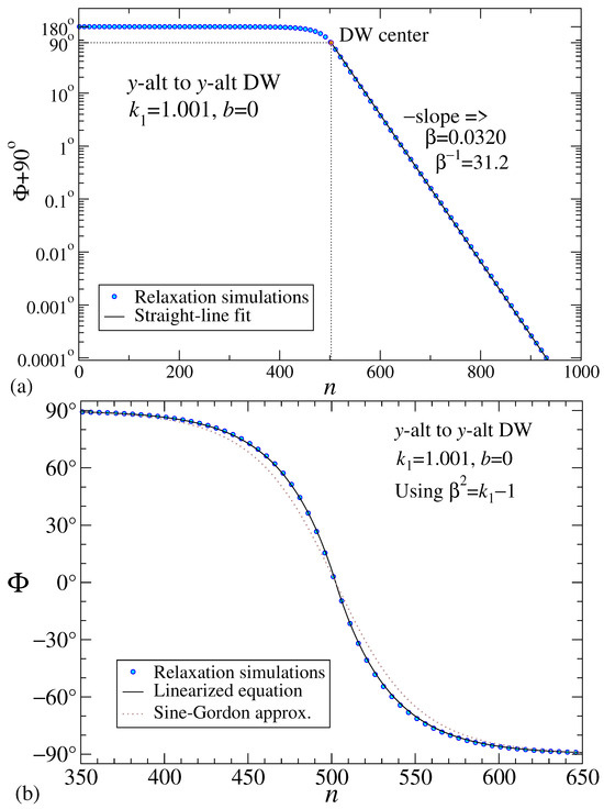
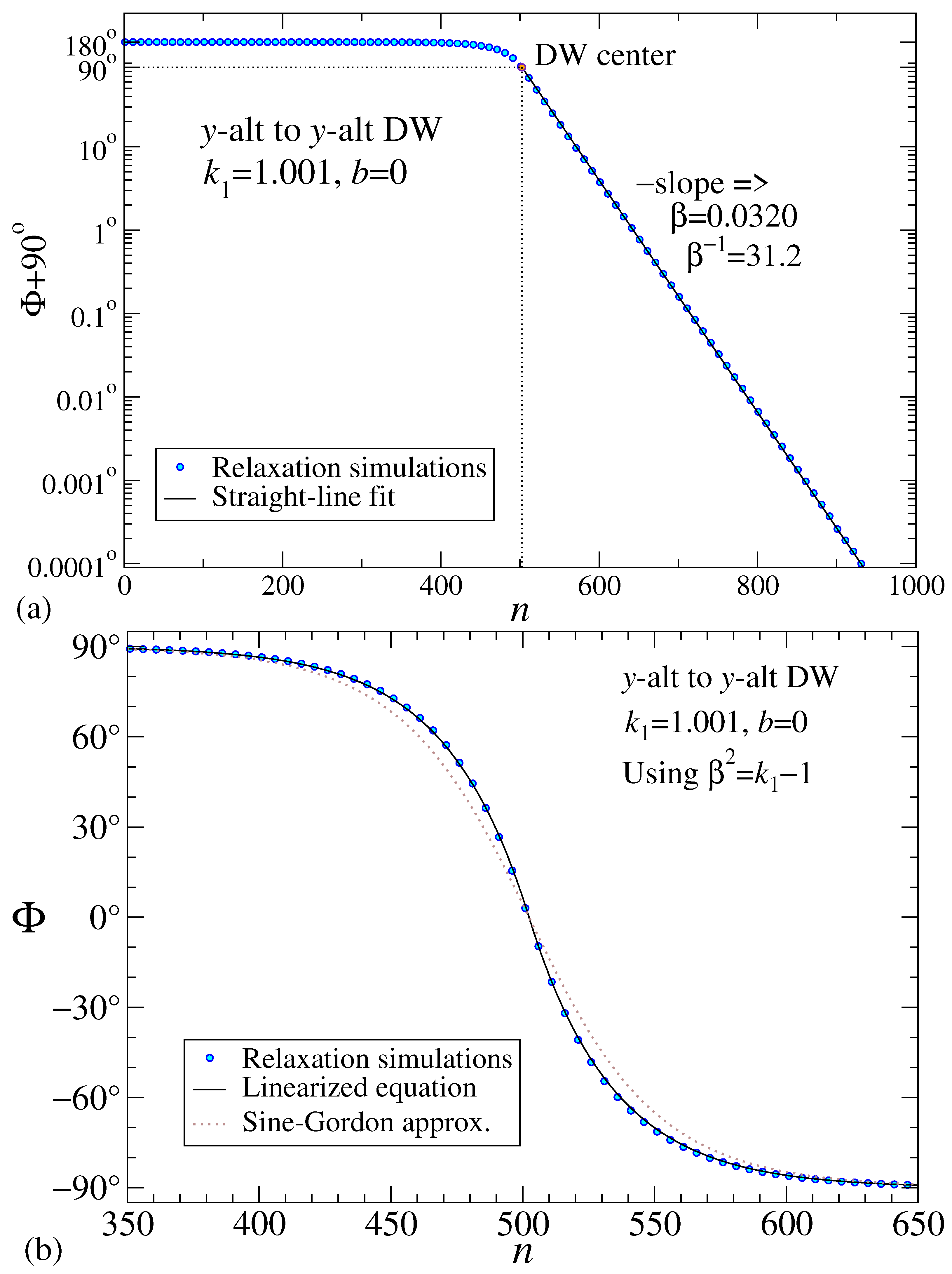
For a DW with $k_1=1.001$ and $b=0$, the asymptotic behavior is displayed in Figure 3a in a log-linear plot. The fitted straight line decay slope ($\beta =0.0320$) is surprisingly close to the continuum prediction from Equation (39), $\beta =0.03162$. The inverse of $\beta$ defines the DW fitted half-width $h\approx 31.2$ (in lattice constants) and the continuum prediction is $h\approx \sqrt{1/0.001}=31.6$, very nearly the same. This large width helps to minimize discreteness effects and make the continuum analysis reliable.

Figure 3. (a) For $k_1=1.001$, $N=1000$, alternating order parameter ${\varphi }_{\mathrm{alt}}$ for a y-alt² DW from the numerical simulations (blue circles) is used to estimate inverse half-width $\beta$ from the negative slope of the log-linear plot, based on Equation (44). Only every tenth site is plotted. The asymptotic function is the black straight line drawn only to the right side of the DW center. The slope came from the DW center point, ${\varphi }_{\mathrm{alt}}\left(502.4\right)=0$, and the far-field point, ${\varphi }_{\mathrm{alt}}\left(934\right)+90=9.0\times {10}^{-5}$. Theory Equation (39) gives $\beta =\sqrt{0.001}\approx 0.03162$. (b) Zoomed-in alternating order ${\varphi }_{\mathrm{alt}}$ of the DW on a linear plot. The numerical simulations are compared with the linear equilibrium Equation (38) and the sine-Gordon approximation in Equation (45). Only every fifth site of the numerical data is plotted.

Of course, the log-linear plot disguises the behavior near the DW center. The linearized theory curve for $\mathrm{\Phi }$ from Equation (40) is shown in Figure 3b, compared to the numerical data and a sine-Gordon approximation (Equation (45)), described below. The linear theory curve fits well at the DW center, and also for $\left|x\right|\to \pm \infty$. The regions with the largest deviation of the theory from the numerical calculation are in the shoulders of the DW, about a distance h from the center, but even those deviations are extremely small.

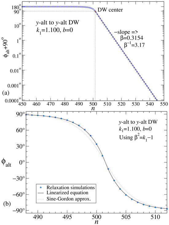
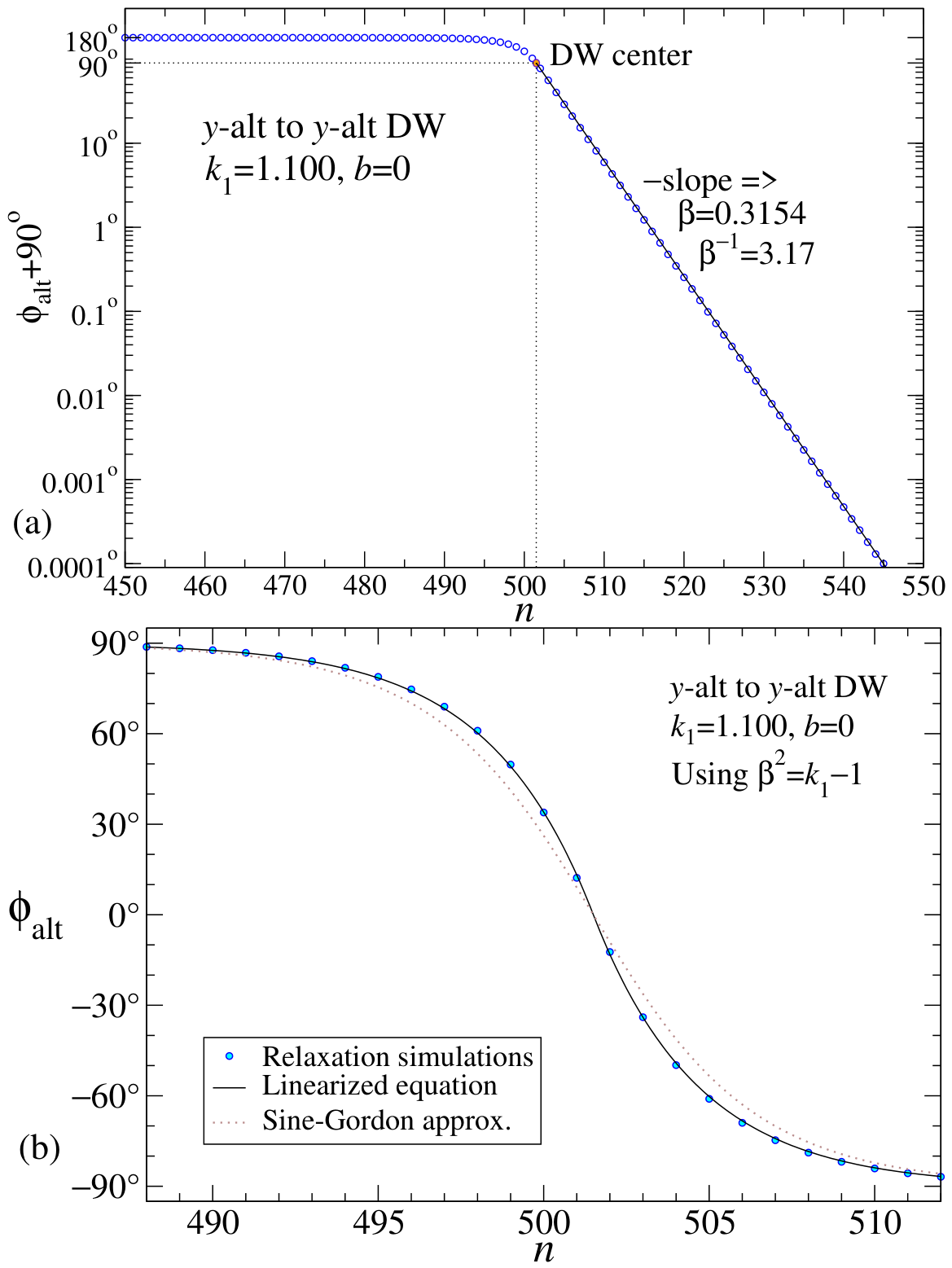
Another static DW was calculated for $N=1000$, $b=0$, and anisotropy $k_1=1.100$, as shown in Figure 4. Although $k_1$ is barely changed from the first example, the factor $k_1-1$ has changed by a factor of 100, which is expected to reduce the half-width by a factor of 1/10th. The asymptotic numerical fit produces $h={\beta }^{-1}\approx 3.17$ while both the linear and sine-Gordon theories predict $h=1/\sqrt{0.100}\approx 3.162$, although it is clear that the sine-Gordon approximation fails in the shoulders of the DW. It is possible to consider larger values of $k_1$ up to $k_1\approx 1.75$; however, by then, the DW acquires a fixed minimum half-width $h_{\min }\approx 1.5$ and a fixed shape and energy, independent of $k_1$ (see Section 7.2).

Figure 4. (a) For $k_1=1.100$, $b=0$, $N=1000$, alternating order ${\varphi }_{\mathrm{alt}}\left(x\right)$ in a y-alt² DW from the numerical simulations (blue circles) is used to estimate $\beta$ from the negative slope of the log-linear plot, based on Equation (44). The asymptotic function is the black straight line drawn only to the right side of the DW center. The slope came from the DW center point, ${\varphi }_{\mathrm{alt}}\left(501.5\right)=0$, and the far-field point, ${\varphi }_{\mathrm{alt}}\left(545.3\right)+90=9.0\times {10}^{-5}$. Theory Equation (39) gives $\beta =\sqrt{0.1}\approx 0.3162$. (b) Zoomed-in view on a linear plot comparing the numerical solution with the linear equilibrium Equation (38) and the sine-Gordon approximation in Equation (45).

7.1. A Sine-Gordon Approximation?

A comparison was made to a sine-Gordon form for the DWs, which actually deviates significantly from the numerical solutions. It is obtained by keeping $sin2\psi$ intact instead of linearizing it. Equation (38) is replaced by

$$(k_1-1)sin\left(2\psi \right)\approx 2{\psi }_{xx}.$$

(45)

One might expect that this gives more accuracy for the determination of the DW. This is a static sine-Gordon equation [21] for the variable $2\psi$. It has static kink solutions. One form that decays away for large positive x is

$$2\psi =4{tan}^{-1}\left(e^{-\beta x}\right),\beta =\sqrt{k_1-1}.$$

(46)

In this formula, $\psi$ ranges from $\pi$ to 0 as x goes from $-\infty$ to $+\infty$. The net result for $\mathrm{\Phi }$ is

$$\begin{array}{cc}\hfill {\mathrm{\Phi }}_{\mathrm{sG}}=-{\displaystyle \frac{\pi }{2}}+\psi & =-{\displaystyle \frac{\pi }{2}}+2{tan}^{-1}\left(e^{-\beta x}\right)\hfill \\ \hfill & =-2{tan}^{-1}\left(tanh\frac{1}{2}\beta x\right).\hfill \end{array}$$

(47)

This applies for $-\infty <x<+\infty$, without absolute value on x. The last expression was found using the identity for a tangent of a difference of angles. While being interesting, it does not closely follow the DW shapes for this model, especially at the shoulders, as seen in Figure 3 and Figure 4. Full linearization must provide a fortuitous cancellation of errors relative to the nonlinear Equation (34).

7.2. DW Creation Energy for $B=0$

The DW creation energy $E^{\ast }$ is the energy needed to push a DW into the system initially in a uniform y-alt state. I take it as the difference of the system energy with a DW minus the energy of a uniform y-alt state. For a static DW, the energy density from Equation (27) with $\mathrm{\Theta }=\vartheta =0$ and $b=0$ is

$${\displaystyle \frac{\mathcal{H}}{D}}=-1-{cos}^2\mathrm{\Phi }+\left(1-\frac{1}{2}{cos}^2\mathrm{\Phi }\right){\mathrm{\Phi }}_x^2-k_1(1-{cos}^2\mathrm{\Phi }).$$

(48)

This is expressed in terms of $cos\mathrm{\Phi }=sin\psi$ [see Equation (35)] for ease of calculation, which gives

$$\begin{array}{cc}\hfill {\displaystyle \frac{\mathcal{H}}{D}}& =-(1+k_1)+(k_1-1){sin}^2\psi +(1-\frac{1}{2}{sin}^2\psi ){\psi }_x^2.\hfill \end{array}$$

(49)

In the solution (40), $\psi$ ranges from 0 to $\pi /2$, ruling out expansion of $\mathcal{H}$ for small or large $\left|\psi \right|$. Instead, I appeal to numerical evaluations of the needed integrals. When $\psi =0$, the first term in the expression is the energy density of a uniform y-alt state,

$${\mathcal{H}}_{y-\mathrm{alt}}/D=-(1+k_1).$$

(50)

The remaining parts of $\mathcal{H}$ give the creation energy,

$${\displaystyle \frac{E^{\ast }}{D}}={\int }_{-\infty }^{\infty }dx\left\{(k_1-1){sin}^2\psi +(1-\frac{1}{2}{sin}^2\psi ){\psi }_x^2\right\}.$$

(51)

With $\psi$ as in Equation (39) and ${\psi }_x^2={\beta }^2{\psi }^2$, the needed integrals are:

$$\begin{array}{cc}\hfill {\int }_{-\infty }^{\infty }dx{\psi }^2& ={\left({\displaystyle \frac{\pi }{2}}\right)}^2{\beta }^{-1}.\hfill \\ \hfill {\int }_{-\infty }^{\infty }dx{sin}^2\psi & \approx 1.6482776{\beta }^{-1}.\hfill \\ \hfill {\int }_{-\infty }^{\infty }dx{\psi }^2{sin}^2\psi & \approx 1.733700{\beta }^{-1}.\hfill \end{array}$$

(52)

Then the net creation energy is predicted to be

$$E^{\ast }/D\approx 3.2488287\beta \approx 3.2488\sqrt{k_1-1}.$$

(53)

Note especially that this does not depend on the length N of the system. The contribution to the energy density is concentrated mostly from shoulder to shoulder in the DW. The formula should work well in a discrete system much longer than the DW width. As $\beta =h^{-1}$, the creation energy is inversely proportional to the DW width. The formula also shows that $k_1=1$ is a critical point below which there are no y-alt² DWs.

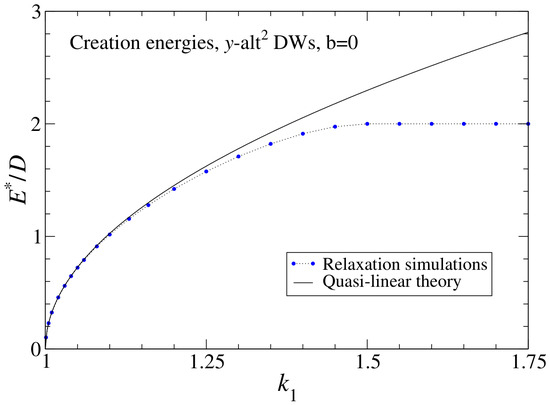
For the first example in Figure 2 with $k_1=1.001$, the formula gives $E^{\ast }\approx 0.10274D$, while the numerical simulations produced $E^{\ast }\approx 0.10265D$. The value from numerics was found using a system with $N=1000$, and subtracting the total energies with and without the DW present in a surrounding y-alt background. It is remarkable that although $\psi$ was obtained from a linearized equation, the energy must be calculated using that linearized but very good solution, taking into account the nonlinearity in the sine functions within $\mathcal{H}$. I refer to this and expression (53) as the quasi-linear theory for the DW energy.

Further creation energies for a range of $k_1>1$ are exhibited in Figure 5. For $k_1<1.25$, the linearized continuum theory for $E^{\ast }$ is only a few percent higher than the values from simulations. In that region, the DW width $w=2h\ge 4$, so that the structure is reliably described using the continuum approach. In contrast, for $k_1\ge 1.5$, the creation energy found from simulations becomes a constant $E^{\ast }=2D$, and the DW takes on a particular discrete shape, of a minimum full-width $w=3$, which cannot be represented adequately in the continuum theory.

Figure 5. The y-alt² DW creation energy vs. anisotropy $k_1$ from simulations (circles) compared with the quasi-linear theory expression in Equation (53) (solid black curve), at zero applied field. For $k_1\ge 1.5$, the DW acquires a minimum width $w=3a$ and a fixed energy $E^{\ast }=2D$, as well as a shape independent of $k_1$. For $k_1<1.25$, the continuum theory works extremely well because the DW width $w=2/\sqrt{k_1-1}$ contains many sites.

8. Continuum Static DWs with Nonzero Magnetic Field

A transverse applied magnetic field $b=\mu B/D$ tends to impart an aligned or ferromagnetic-like order to the DW, which should obey the equilibrium Equation (34). This can be analyzed starting again with the large-$\left|x\right|$ transformation to variable $\psi \left(x\right)\ge 0$ in Equation (35). Assuming ${\psi }^2\ll 1$, one has $cos2\mathrm{\Phi }\approx 3+k_1$ and the field contribution to the equilibrium equation is simplified, giving

$$(2-{\psi }^2){\psi }_{xx}-\left[k_1-1-{\displaystyle \frac{b^2}{4(3+k_1)}}+\frac{1}{2}{\psi }_x^2\right]\left(2\psi \right)\approx 0.$$

(54)

Asymptotically, the fifth-order small terms can be dropped, and the DW is still described by a linearized equilibrium equation,

$${\psi }_{xx}\approx \left[k_1-1-{\displaystyle \frac{b^2}{4(3+k_1)}}\right]\psi .$$

(55)

The field term effectively subtracts from the $k_1$ anisotropy. The solution is similar to that for zero field, but with a modified inverse half-width parameter,

$$\psi ={\displaystyle \frac{\pi }{2}}{e}^{-\beta \left|x\right|},\beta =\sqrt{k_1-1-{\displaystyle \frac{b^2}{4(3+k_1)}}}=h^{-1}.$$

(56)

A typical DW is described by Equation (40) or one of the other symmetries. $\phi$ is then determined by Equation (33) or equivalently,

$$\phi ={\displaystyle \frac{bsin\psi }{2(3+k_{1}cos2\psi )}}.$$

(57)

At the DW center, where $\mathrm{\Phi }=0$ and $\psi ={\displaystyle \frac{\pi }{2}}$, the maximum tilt towards the applied field is

$$\phi \left(0\right)={\phi }_{\max }\approx {\displaystyle \frac{b}{2(3-k_1)}}.$$

(58)

To ensure real $\beta$, the field must be less than an upper critical limit,

$$b_c=\sqrt{4(k_1-1)(3-k_1)}.$$

(59)

For example, when $k_1=1.25$, one has $b_c=1.32$, and then ${\phi }_{\max }\approx 0.38$ rad. That is at a stability limit and a more typical value for a stable y-alt² DW is only a few degrees.

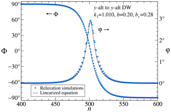
To compare with numerical simulations, both the alternating order and aligned order is to be extracted from a relaxed DW configuration. The ferromagnetic-like order can be estimated at a site by a slight modification of the Formula (43) used to find the alternating order. We use an average over the sublattices,

$${\varphi }_{\mathrm{fm},n}=\frac{1}{2}[{\varphi }_n+\frac{1}{2}({\varphi }_{n-1}+{\varphi }_{n+1})].$$

(60)

This is the discrete measurement on the simulation data, to be directly compared to the analytic estimate of $\phi$.

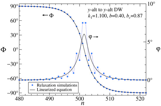
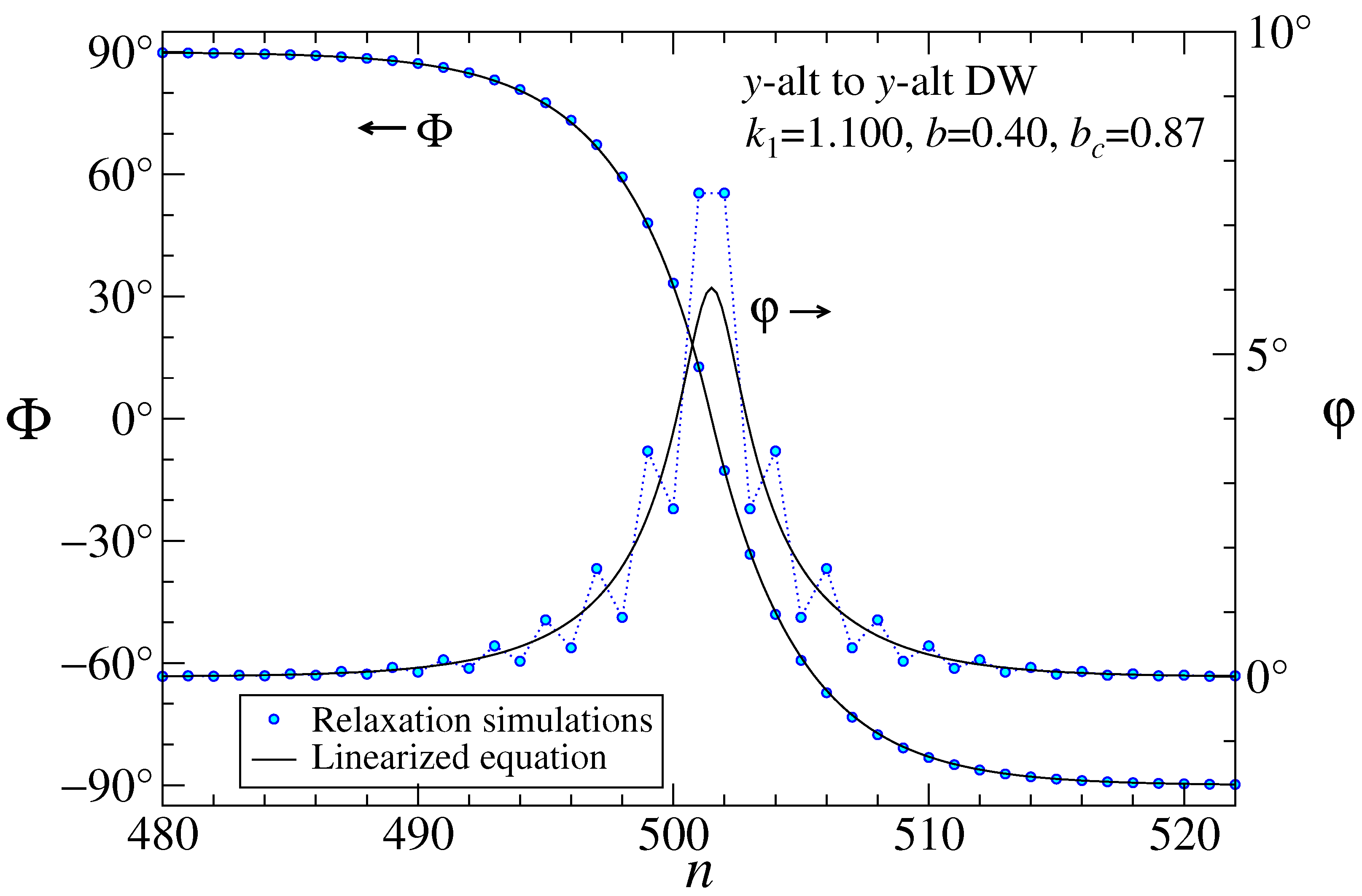
The theory matches the simulations exceptionally well at $k_1=1.001$ as used in an earlier example with $b=0$. To see some slights deviations between theory and simulations, an example of a DW for $k_1=1.010$, $b_c=0.2821$, and $b=0.20$ is shown in Figure 6. The agreement is still very good, although the central peak in the theory curve for $\phi$ is slightly narrower than the central peak in the simulation data. A site-by-site variation in $\phi$ is also noticeable as there are slight discreteness effects in the data.

Figure 6. For $k_1=1.01$ and $b=0.20$, a y-alt to y-alt DW from the numerical simulations with $N=1000$ is compared with the theoretical shape from Equations (40) and (57). For the theory curves, the DW center was placed at $x=502$ to match the data.

It is interesting to check another example with $k_1=1.100$, $b_c=0.8718$, and $b=0.40$ as shown in Figure 7. The larger field creates a greater peak deviation. Discreteness effects are strong and the smooth continuum theory for $\phi$ passes through the average of the site-to-site oscillations of the simulation data, except at the peak. As long as b is not too close to the critical limit $b_c$, these examples show that the continuum theory using the linearized equilibrium equation is good at describing the DW structures.

Figure 7. For $k_1=1.100$ and $b=0.40$, a y-alt to y-alt DW from the numerical simulations with $N=1000$ is compared with the theoretical shape from Equations (40) and (57). A dotted line is used to distinguish the simulation data for $\phi$. For the theory curves, the DW center was placed at $x=502$ to match the data.

8.1. Longitudinal Magnetic Moment $M_x$ of a DW

A y-alt² DW has a net magnetic moment $m_x$ parallel to the chain direction, with positive and negative values that are only slightly dependent upon the applied field b. The discrete and continuum definitions in spin units are

$$m_x\equiv \sum _n{S}_n^x={\int }_{-\infty }^{+\infty }{\displaystyle \frac{dx}{a}}⟨S_n^x⟩.$$

(61)

The average is over the sublattices, both of which have nearly the same $S_n^x$. In the continuum opposing rotations scenario for the two sublattices, they are

$$S_n^x=cos(\pm \mathrm{\Phi }+\phi )\approx cos\mathrm{\Phi }\left(1-\frac{1}{2}{\phi }^2\right)-sin(\pm \mathrm{\Phi })\left(\phi \right).$$

(62)

Then the average is

$$⟨S_n^x⟩\approx cos\mathrm{\Phi }\left(1-\frac{1}{2}{\phi }^2\right).$$

(63)

In the DW, the asymptotic solution has $cos\mathrm{\Phi }=sin\psi$, and using the value already found for $\phi$ in Equation (57), we have

$$⟨S_n^x⟩\approx sin\psi \left[1-{\displaystyle \frac{b^2{sin}^2\psi }{8{(3+k_{1}cos2\psi )}^2}}\right].$$

(64)

Using $cos2\psi \approx 1$, the net $m_x$ depends on integrals over x or over $\psi$ that are evaluated numerically:

$$\begin{array}{cc}\hfill {\int }_{-\infty }^{\infty }dxsin\psi & =2{\int }_0^{{\displaystyle \frac{\pi }{2}}}{\displaystyle \frac{d\psi }{|d\psi /dx|}}sin\psi \approx 2.741{\beta }^{-1}.\hfill \\ \hfill {\int }_{-\infty }^{\infty }dx{sin}^3\psi & =2{\int }_0^{{\displaystyle \frac{\pi }{2}}}{\displaystyle \frac{d\psi }{|d\psi /dx|}}{sin}^3\psi \approx 1.252{\beta }^{-1}.\hfill \end{array}$$

(65)

That gives the estimate for the magnitude,

$$\left|m_x\right|\approx \left[2.74-{\displaystyle \frac{1.25b^2}{8{(3+k_1)}^2}}\right]{\beta }^{-1}\approx 2.74{\beta }^{-1}.$$

(66)

With $k_1\approx 1$, the term with $b^2$ is negligible, although $\beta$ has implicit b-dependence. A positive or negative value of $m_x$ is allowed, slightly more than the DW width. This is fairly large and could be used to distinguish the DW-state from a uniform y-alt state with $m_x=0$.

8.2. Transverse Magnetic Moment of a DW

The magnetic field induces a net transverse magnetic moment in the dipoles in a DW. The net induced moment is defined in discrete and continuum views by

$$m_y\equiv \sum _n{S}_n^y={\int }_{-\infty }^{+\infty }dx⟨S_n^y⟩.$$

(67)

Outside the DW, $S^y$ decays exponentially. With the main contribution from the center of the DW, the asymptotic DW solution (56) can give an estimate. From the calculation of the continuum Hamiltonian and Equation (A56) with $\mathrm{\Theta }=\vartheta =0$, the transverse spin component averaged over the sublattices is

$$⟨S_n^y⟩\approx \phi cos\mathrm{\Phi }={\displaystyle \frac{b{sin}^2\psi }{2(3+k_{1}cos2\psi )}}.$$

(68)

Integration over x can be changed to integration over $\psi$, together with using the asymptotic approximations $sin\psi \approx \psi$ and $cos2\psi \approx 1$. This gives the net linearized continuum prediction,

$$m_y\approx 2{\int }_{\psi =0}^{\psi =\pi /2}{\displaystyle \frac{d\psi }{|d\psi /dx|}}{\displaystyle \frac{b{\psi }^2}{2(3+k_1)}}={\displaystyle \frac{{\pi }^{2}b}{8(3+k_1)\beta }}.$$

(69)

Note that ${\psi }^2$ is an overestimate of ${sin}^2\psi$ in the numerator, while the denominator is also overestimated; these errors tend to cancel.

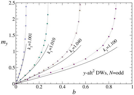
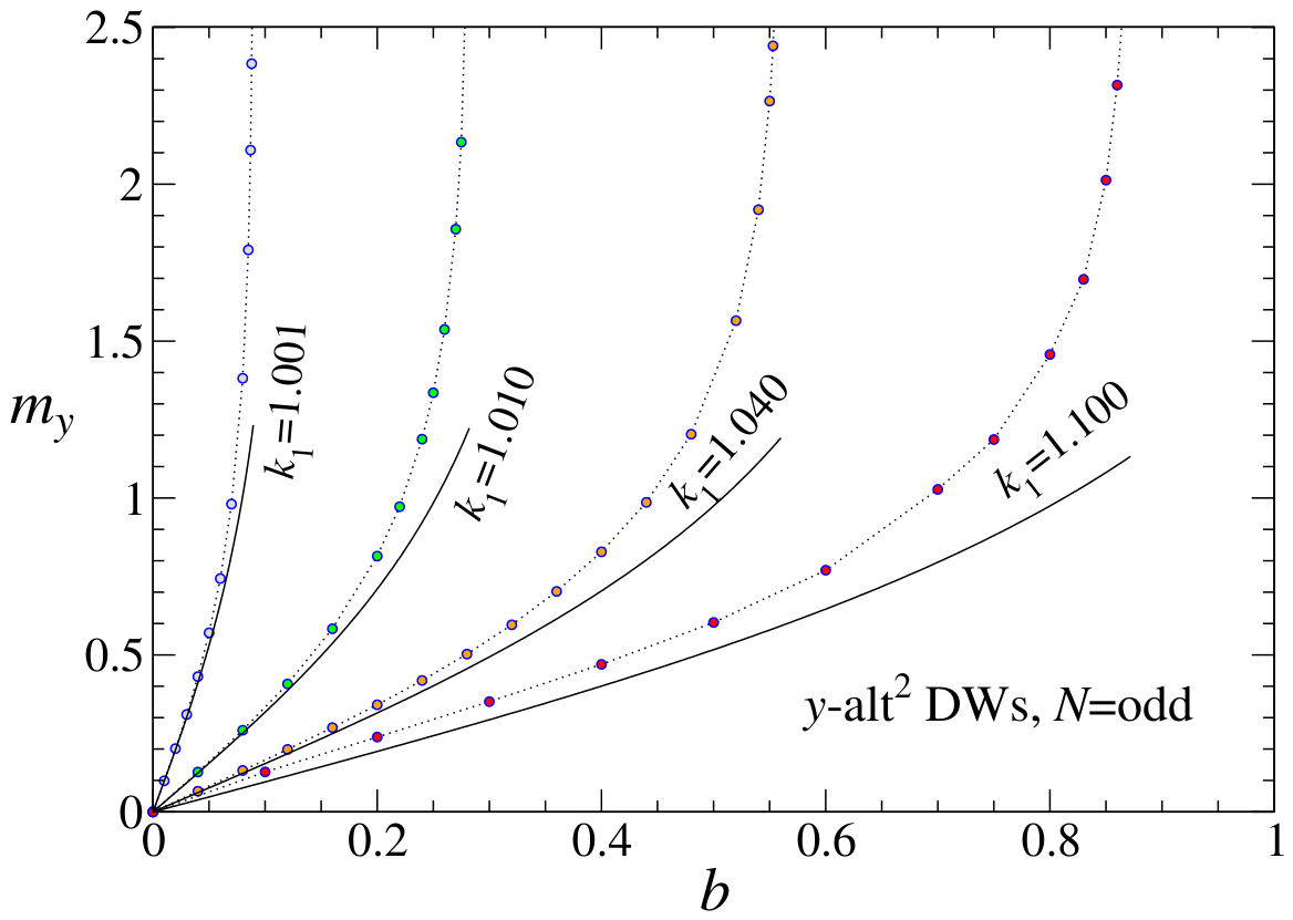
For the example with $k_1=1.01,b=0.20$, one gets $\beta =0.0866$, and the formula gives $m_y\approx 0.710$, while the simulated values are interesting. If the system contains an odd number of sites (say, $N=501$), the simulated value is $m_y=0.815$, a component aligned paramagnetically with the field, but somewhat larger than the theory prediction. A comparison of $m_y$ obtained from the simulations and the theory for odd-N is shown in Figure 8. Generally the theory expression underestimates $m_y$ and works best for the smaller values of $k_1$.

Figure 8. The induced transverse magnetic moment $m_y$ of a y-alt² DW in applied magnetic field b, for the indicated anisotropy strengths. Points are from simulations of odd-numbered chains ($N=501$), dotted lines are guides to the eye, and the solid black curves are the linearized theory expression in Equation (69). For an even-N chain, the results for $m_y$ are shifted from these by the quantized intrinsic moment, $m_y=\pm 1$.

If instead the system contains an even number of sites (say, $N=500$), the simulated value can be either $m_y=1.815=1+0.815$ or $m_y=-0.185=-1+0.815$, depending on the initial state of the simulation. In both cases, the DW remains in the center of the system. The negative value of $m_y$ means it points opposite to the applied field. The two cases correspond to opposite directions of rotation in the spins as one moves down the chain. The magnetic moment is shifted from that for the odd-N system by a quantized topological value, $m_y^{\mathrm{topo}}=\pm 1$.

Surprisingly, if $b=0$, the DW in an even-N chain can have one of the exactly quantized intrinsic values, $m_y=m_y^{\mathrm{topo}}=\pm 1$. This topological effect is not correctly accounted for in the continuum theory. It does not appear in odd-N chains. Equation (69) for $m_y$ induced by b applies directly only for odd-N chains. For even-N chains, Equation (69) represents the field-induced magnetic moment that takes place on top of the intrinsic values of $m_y^{\mathrm{topo}}=\pm 1$. To get $m_y$ for even-N chains, one can take the values plotted in Figure 8 and shift them by the intrinsic values, $\pm 1$.

8.3. On Odd-Length vs. Even-Length Chains

The odd/even chain effect is accounted for by carefully examining the configurations in short-chain DWs ($N=49$ or 50).

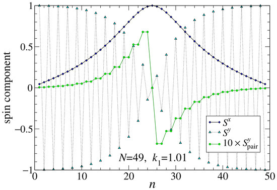
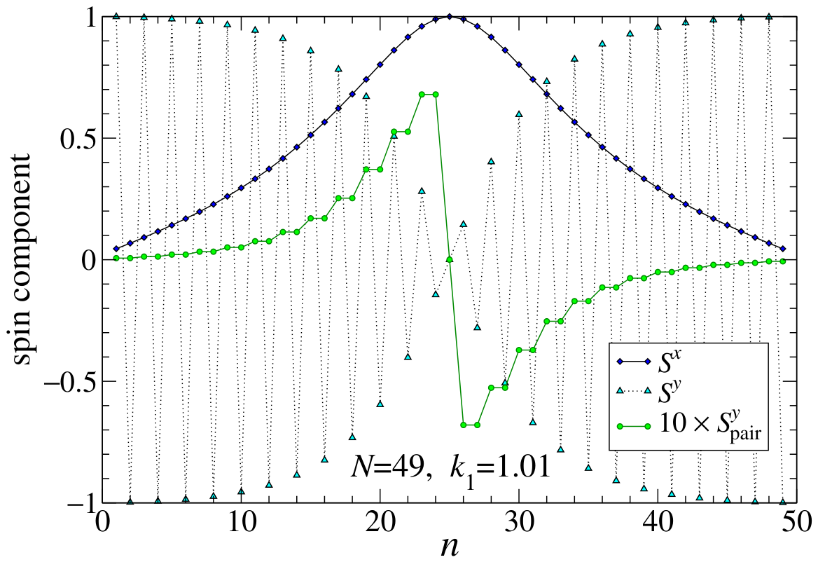
In an odd chain with $b=0$, there is a centered site with $S_n^y=0$, around which $S_n^y$ holds antisymmetry on each sublattice. An example is shown in Figure 9 for $N=49$, $k_1=1.01$, where the raw spin components $S_n^x,S_n^y$ on the islands are shown. $S_n^x$ is the same for both sublattices, but $S_n^y$ alternates from site to site. It is difficult to visualize the sum of $S_n^y$ to get the net $m_y$. I calculated a pair average to make it apparent. The average is taken over pairs of neighboring odd/even sites,

$$S_{\mathrm{pair},n}^y=S_{\mathrm{pair},n+1}^y=\frac{1}{2}(S_n^y+S_{n+1}).$$

(70)

Each site in a pair is given the same average value. With $N=$ odd, one site is not in a pair; it is taken as the site at the center of the DW, which happens also to have $S_{25}^y=0$. On the left side of the center, the pairs are odd–even, or (n)-($n+1$) being 1-2, 3-4, 5-6, etc. On the right side of the center, the pairs are even–odd, or (n)-($n+1$) being 26-27, 28-29, 30-31, etc. Now the sum is clear, and the two antisymmetric halves can be seen to cancel out and give $m_y=\sum S_{\mathrm{pair},n}^y=0$.

Figure 9. A DW spin configuration for odd system length $N=49$, anisotropy $k_1=1.01$, field $b=0$, from relaxation simulations. $S_n^x$ and $S_n^y$ are the raw components on the islands. Note the alternating structure present in $S_n^y$. The values of $S_{\mathrm{pair},n}^y$ are the averages of odd/even neighboring sites in each two-site pair, but the DW center site with $S_n^y=0$ at $n=25$ is plotted individually. The antisymmetry of $S_{\mathrm{pair},n}^y$ leads to net $m_y=0$.

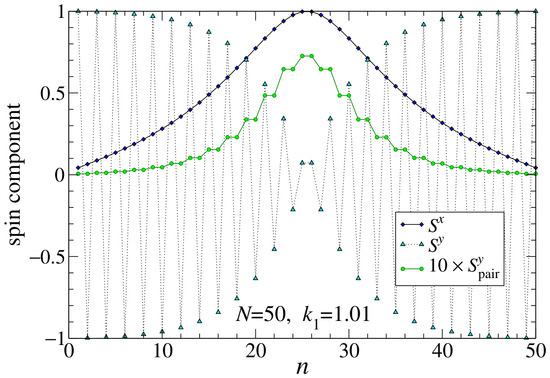
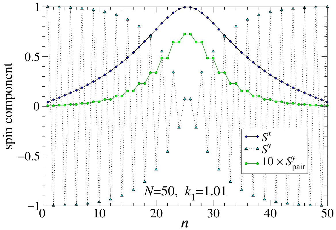
In an even chain with $b=0$, the center of the DW falls between two sites. An example with $N=50$, $k_1=1.01$, and $b=0$ is shown in Figure 10, displaying the raw $S_n^x$ and $S_n^y$ and the pair-averaged $S_{\mathrm{pair},n}^y$. In this case, all of the pairs are of the form odd–even, or 1–2, 3–4, 5–6, etc., across the whole length of the system. There is no site not in a pair. It is clear that $S_{\mathrm{pair},n}^y$ now has right/left symmetry around the DW center, and the two halves make equal contributions to the net $m_y$ even though $b=0$. It creates a nonzero, quantized, intrinsic magnetic moment $m_y=\pm 1$. This is the topological effect, caused by the addition of one (up or down) spin to an odd-N chain. If an odd-N chain has $m_y=0$, then the even-N chain must have $m_y=m_y^{\mathrm{topo}}=\pm 1$, because the spins are all $S_n^y=\pm 1$ in the y-alt states at the chain ends, far from the DW center.

Figure 10. A DW spin configuration for even system length $N=50$, anisotropy $k_1=1.01$, field $b=0$, from relaxation simulations. See explanation of curves in Figure 9 for $N=49$. Now all sites are in pairs, and $S_{\mathrm{pair}}^y$ is symmetric around the DW center. The net intrinsic magnetic moment is $m_y=1$, even though $b=0$.

This way of summing by pairs, and leaving the central site of an odd-N system unpaired, is a way to move all the contributions to $m_y$ away from the boundaries, which are in y-alt states. It makes the odd/even influence come from the DW itself. In this sense, a boundary effect has been recast as a surprising geometric property of the DW.

This method contradicts the original approach of the continuum limit, because what appears in these pairs depends on where their construction starts. A shift by 1 site leaves some spin unpaired. Further, the intrinsic magnetic moment for even-N systems does not emerge in the original continuum limit, even though it seems to come mostly from the DW central region. Instead, $S_{\mathrm{pair},n}^y$ can be averaged over sublattices and summed to produce the intrinsic part of $m_y$.

The continuum version of $S_{\mathrm{pair},n}^y=S_{\mathrm{pair},n+1}^y$ depends on whether n is even or odd. First, consider $n=$ even, and use the opposing rotations assumption in the planar case,

$$\begin{array}{cc}\hfill S_{\mathrm{pair},n}^y& =S_{\mathrm{pair},n+1}^y=\frac{1}{2}(S_n^y+S_{n+1}^y)\hfill \\ \hfill & \to \frac{1}{2}\left[sin\mathrm{\Phi }\left(x\right)+sin(-\mathrm{\Phi }(x+a\left)\right)\right]\hfill \\ \hfill & =\frac{1}{2}\left[sin\mathrm{\Phi }-sin(\mathrm{\Phi }+a{\mathrm{\Phi }}_x+\frac{1}{2}{a}^2{\mathrm{\Phi }}_{xx})\right]\hfill \\ \hfill & \approx -\frac{1}{2}a{\mathrm{\Phi }}_{x}cos\mathrm{\Phi },n=\mathrm{even}.\hfill \end{array}$$

(71)

If $n=$ odd, the sign of $\mathrm{\Phi }$ is reversed, leaving

$$S_{\mathrm{pair},n}^y=S_{\mathrm{pair},n+1}^y\approx \frac{1}{2}a{\mathrm{\Phi }}_{x}cos\mathrm{\Phi },n=\mathrm{odd}.$$

(72)

Thus, an odd–even pair has a different sign from an even–odd pair. This explains the antisymmetry seen in the odd-N chain, which has odd–even pairs on one side of the center and even–odd pairs on the other side. For the even-N chain, all the pairs are odd–even (use $n=$ odd formula) and then right–left symmetry is the result.

Thus, we can use the result and the asymptotic DW solution to find the intrinsic magnetic moment for even-N chains. Consider a DW with $\mathrm{\Phi }(-\infty )=-{\displaystyle \frac{\pi }{2}}$ and $\mathrm{\Phi }(+\infty )={\displaystyle \frac{\pi }{2}}$. The continuum expression for $S_{\mathrm{pair},n}^y$ with $n=$ odd is a perfect differential, so its integration does not depend on the details of the DW shape. This is the reason why the intrinsic $m_y$ is quantized, and the value is obtained by

$$\begin{array}{cc}\hfill m_y^{\mathrm{topo}}& =\sum _n{S}_{\mathrm{pair},n}^y\to {\int }_{-\infty }^{\infty }{\displaystyle \frac{dx}{a}}\frac{1}{2}a{\displaystyle \frac{d\mathrm{\Phi }}{dx}}cos\mathrm{\Phi }\hfill \\ \hfill & =\frac{1}{2}{\int }_{-\infty }^{\infty }dx{\displaystyle \frac{d}{dx}}(sin\mathrm{\Phi })\hfill \\ \hfill & =\frac{1}{2}\left[sin\mathrm{\Phi }(\infty )-sin\mathrm{\Phi }(-\infty )\right]=1.\hfill \end{array}$$

(73)

With the DW flipped (reverse all spins), one instead gets $m_y^{\mathrm{topo}}=-1$. This quantization of $m_y$ for even-N chains with $b=0$ is indeed exact.

If it is an odd-N chain, the left half of the system uses $S_{\mathrm{pair},n}^y$ with $n=$ odd and the right half uses it with $n=$ even. They have reversed signs, and their left vs. right side sums cancel out upon integration over the whole chain, as seen in Figure 9. The odd-N chains have intrinsic $m_y=0$, exactly.

When $b\ne 0$, the continuum prediction of $m_y$ (Equation (69)) is superimposed onto the intrinsic value, whether it be an odd-N or even-N chain. This analysis explains how topological effects influence the values of $m_y$ differently for even-N vs. odd-N chains.

8.4. DW Creation Energy for $B\ne 0$

When a transverse field is present, the continuum energy density in a static DW from Equation (27) with $\mathrm{\Theta }=\vartheta =0$ now includes terms in the small angle $\phi$,

$$\begin{array}{cc}\hfill {\displaystyle \frac{\mathcal{H}}{D}}& =-1-{cos}^2\mathrm{\Phi }+\left(1-\frac{1}{2}{cos}^2\mathrm{\Phi }\right){\mathrm{\Phi }}_x^2+3{\phi }^2\hfill \\ \hfill & -k_1(1-{cos}^2\mathrm{\Phi }+{\phi }^{2}cos2\mathrm{\Phi })-b\phi cos\mathrm{\Phi }.\hfill \end{array}$$

(74)

This accounts for the induced magnetic moment, but not an intrinsic one. Using the asymptotic DW solution (Equations (56) and (57)), this can be written

$$\begin{array}{cc}\hfill {\displaystyle \frac{\mathcal{H}}{D}}& =-(1+k_1)+(k_1-1){sin}^2\psi \hfill \\ \hfill & +(1-\frac{1}{2}{sin}^2\psi ){\psi }_x^2-{\displaystyle \frac{b^2{sin}^2\psi }{4(3+k_{1}cos2\psi )}}.\hfill \end{array}$$

(75)

The first term is the uniform y-alt energy density, which is to be subtracted out to get the DW creation energy. The Oersted field term can benefit from an expansion for $sin\psi \ll 1$,

$${\displaystyle \frac{1}{3+k_{1}cos2\psi }}\approx {\displaystyle \frac{1}{3+k_1}}\left(1+{\displaystyle \frac{2k_1}{3+k_1}}{sin}^2\psi \right).$$

(76)

Then the continuum DW creation energy is an integral of the energy density over the system,

$$\begin{array}{cc}\hfill {\displaystyle \frac{E_{\mathrm{con}}^{\ast }}{D}}=& {\int }_{-\infty }^{\infty }dx\{(k_1-1){sin}^2\psi +(1-\frac{1}{2}{sin}^2\psi ){\psi }_x^2\hfill \\ \hfill & -{\displaystyle \frac{b^2{sin}^2\psi }{4(3+k_1)}}\left(1+{\displaystyle \frac{2k_1}{3+k_1}}{sin}^2\psi \right)\}.\hfill \end{array}$$

(77)

With a substitution based on Equation (56),

$$k_1-1={\beta }^2+{\displaystyle \frac{b^2}{4(3+k_1)}},$$

(78)

the integrals of ${sin}^2\psi$ proportional to $b^2$ cancel out. The dipolar parts have been integrated earlier in Equation (52). The field contribution now depends on an integral evaluated numerically,

$${\int }_{-\infty }^{\infty }dx{sin}^4\psi \approx 1.03886429{\beta }^{-1}.$$

(79)

Combining all contributions, we see that the preliminary formula for continuum creation energy is the zero field Formula (53), reduced by an Oersted term quadratic in the field,

$${\displaystyle \frac{E_{\mathrm{con}}^{\ast }}{D}}\approx 3.2488\beta -1.03886{\displaystyle \frac{k_1{b}^2}{2{(3+k_1)}^2\beta }}.$$

(80)

The inverse half-width $\beta$ also diminishes with increasing $b^2$. This preliminary formula only involves the induced magnetic moment $m_y$ and not any topological magnetic moment.

To compare with $E^{\ast }$ in simulations, some care is needed, due to the topological magnetic moment for DWs in even-N chains and not in odd-N chains. The creation energy is the difference of the system energy with the DW present, minus the system energy in a uniform y-alt state, accounting correctly for intrinsic magnetic moments.

If N is even, the DW state has the induced field whose Oersted energy is included in Equation (80) as a term dependent on $b^2$, plus a contribution due to the topological magnetic moment, $m_y^{\mathrm{topo}}\left(\mathrm{DW}\right)=\pm 1$. The contribution of a topological or intrinsic magnetic moment has been left out of Equation (80). The extra topological Oersted energy contribution is $-b{m}_y^{\mathrm{topo}}\left(\mathrm{DW}\right)$. Also note that the uniform y-alt state for even N has no topological magnetic moment, as all spins are in up–down pairs.

If N is odd, the DW state has the induced field whose Oersted energy is included in Equation (80), but there is no topological magnetic moment. However, for an odd chain, the y-alt state whose energy must be subtracted does have one unmatched spin, either up or down along y, giving it a topological magnetic moment $m_y^{\mathrm{topo}}\left(y\text{-}\mathrm{alt}\right)=\pm 1$. The corresponding energy contribution to the y-alt state is $-b{m}_y^{\mathrm{topo}}\left(y\text{-}\mathrm{alt}\right)$, which is to be subtracted out from $E_{\mathrm{con}}$.

Then the net creation energy for both even-N and odd-N chains can be written with a single formula,

$${\displaystyle \frac{E^{\ast }}{D}}\approx 3.2488\beta -1.03886{\displaystyle \frac{k_1{b}^2}{2{(3+k_1)}^2\beta }}-b\Delta m_y^{\mathrm{topo}}.$$

(81)

The topological term is expressed with the change in topological magnetic moment upon DW formation out of the y-alt state, defined as

$$\Delta m_y^{\mathrm{topo}}\equiv m_y^{\mathrm{topo}}\left(\mathrm{DW}\right)-m_y^{\mathrm{topo}}\left(y\text{-}\mathrm{alt}\right).$$

(82)

Physically, that is the intrinsic magnetic moment carried into the system by the DW, if one imagined it entering at one end of a long chain initially in a y-alt state. It cannot enter any other way without tearing the texture. The creation energy formula predicts a combination of linear and roughly quadratic dependencies on b, with strongly different slopes as determined by $\Delta m_y^{\mathrm{topo}}=\pm 1$.

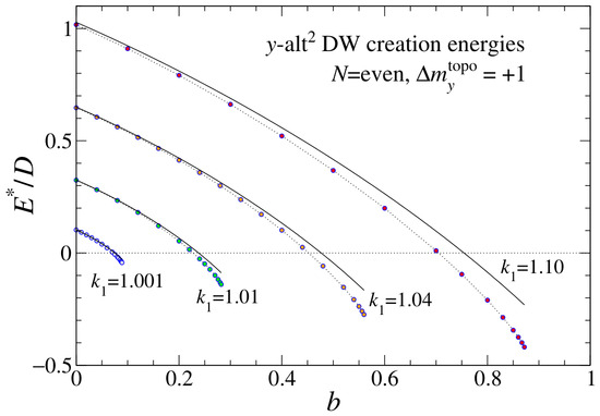
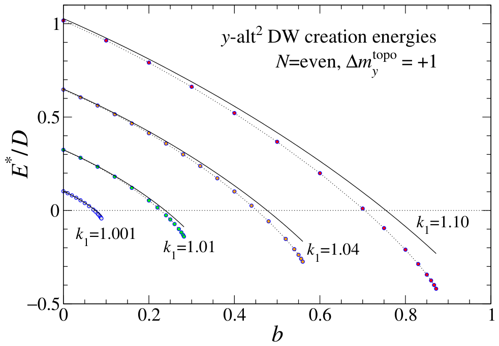
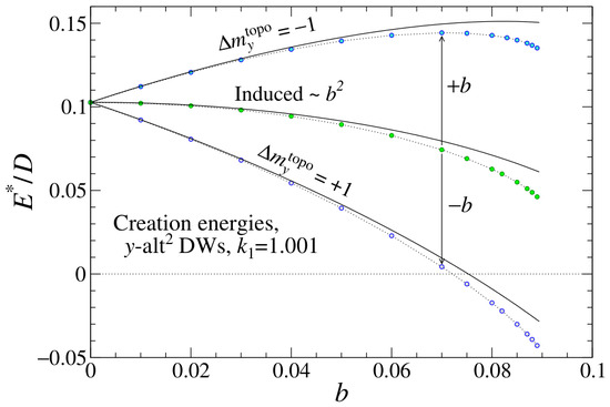
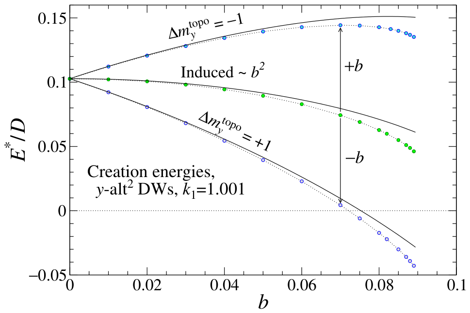
Figure 11 shows a comparison of the creation energies from simulations with this theoretical expression for $\Delta m_y^{\mathrm{topo}}=+1$, which means even chains where the DW has $m_y^{\mathrm{topo}}\left(\mathrm{DW}\right)=+1$ or odd chains where the initial state has $m_y^{\mathrm{topo}}\left(y\text{-}\mathrm{alt}\right)=-1$. Note how $E^{\ast }$ has a noticeable negative slope, due to the topological term, whose explanation is elusive without realizing that the continuum theory only includes the part of $m^y$ induced by the field. The simulated energies are less than the theoretical values, as the configuration can deform away from the theoretical shape to better minimize its energy. Indeed, at large enough b, the creation energies become negative, and the DW state has a lower energy than the uniform y-alt state.

Figure 11. Creation energy of a y-alt² DW in applied magnetic field b, for various anisotropy strengths, even N, and $m_y^{\mathrm{topo}}\left(\mathrm{DW}\right)=+1$ in the DW state, or $\Delta m_y^{\mathrm{topo}}=+1$. Points are from simulations of chains with 500 or 800 sites, dotted lines are guides to the eye, and the solid black curves are the theory expression in Equation (81), which accounts for the topological Oersted energy shift of the DW state.

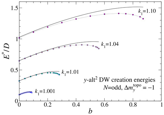
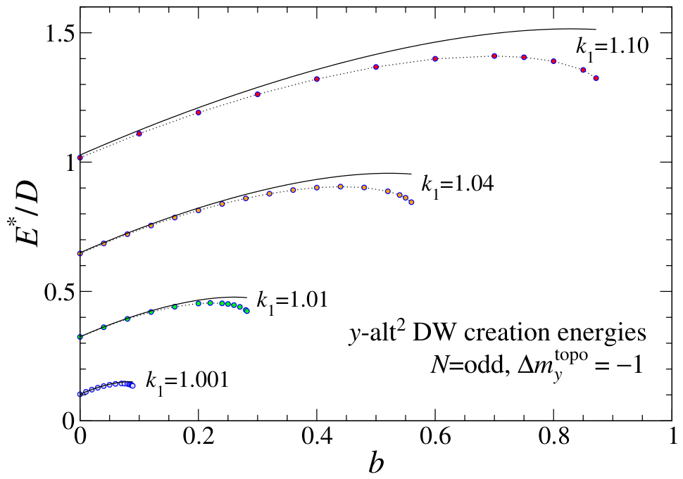
Further results are seen in Figure 12 for $\Delta m_y^{\mathrm{topo}}=-1$, which means even chains where the DW has $m_y^{\mathrm{topo}}\left(\mathrm{DW}\right)=-1$ or odd chains where the initial state has $m_y^{\mathrm{topo}}\left(y\text{-}\mathrm{alt}\right)=+1$. Now the creation energy vs. b initially has a positive slope due to the topological term. The creation energy in this case does not become negative for any of the examples used. For both signs of $\Delta m_y^{\mathrm{topo}}$, the theory works best for values of $k_1$ as close as possible to unity, where a continuum view of the system is best (wide DWs).

Figure 12. Creation energy of a y-alt² DW in applied magnetic field b, for various anisotropy strengths, odd N, and $m_y^{\mathrm{topo}}\left(y\text{-}\mathrm{alt}\right)=+1$ in the reference y-alt state, or $\Delta m_y^{\mathrm{topo}}=-1$. Points are from simulations of chains with 501 or 801 sites, dotted lines are guides to the eye, and the solid black curves are the theory expression in Equation (81), which accounts for the topological Oersted energy shift of the odd-chain y-alt reference state.

It is also interesting to directly compare the creation energies for $\Delta m_y^{\mathrm{topo}}=\pm 1$. At $k_1=1.001$, that is shown in Figure 13. The curves start at the same point for $b=0$ and then separate by a difference of $2b$ for increasing field. Each curve is shifted away from an average curve (the energy of the induced magnetic moment) described by Equation (80) by $\pm b$ due to the topological effects.

Figure 13. Creation energy of y-alt² DWs vs. applied magnetic field b, for $\Delta m_y^{\mathrm{topo}}=\pm 1$ at a selected anisotropy. Points are from simulations with $N=501$ and $\Delta m_y^{\mathrm{topo}}=-1$ (upper) and with $N=500$ and $\Delta m_y^{\mathrm{topo}}=+1$ (lower). Dotted curves are guides to the eye, and the solid black curves are the theory expressions in Equation (81), which include the topological Oersted energy shifts, indicated by arrows. The intermediate data and curve show simulations and theoretical Equation (80) that contain the energy contributions due to induced magnetic moment without topological effects.

9. Discussion and Conclusions

The 1D chain of transverse magnetic islands analyzed here has been shown to have pairs of degenerate uniform states, between which domain walls can form. For the pair of almost indistinguishable uniform y-alt states, such as those present at opposite ends in Figure 1, the DW imposes a rotation of the dipoles on alternating sites in opposing senses in the $xy$ plane. This was found initially via numerical simulations that relax the system from an initial abrupt DW towards one that is spread out and a local energy minimum. In static equilibrium, the dipoles lie in the $xy$ plane, each parallel to the effective field ${\mathbf{B}}_n$ in Equation (3) that acts on it.

Due to that rotation within the DW, a large net magnetic moment $m_x$ parallel to the chain emerges under this opposing rotations scenario. Its magnitude in spin units is of the order of the DW full-width, as estimated in Equation (66). If there also happens to be an applied magnetic field transverse to the chain, that also induces a weaker transverse magnetic moment $m_y$, whose magnitude increases nonlinearly with the field strength, as in Figure 8.

For the simplest continuum analysis, NN dipolar interactions together with island anisotropies have been considered. A set of continuum limit equations of motion for the dipolar angles was found after tedious calculations in two different ways for verification: (1) expansion of the discrete dynamic equations, and (2) by derivation from a continuum Hamiltonian. These derivations used the assumption of opposing rotations on the two sublattices, which is in contrast to an opposing directions assumption that is traditionally used for antiferromagnets. This difference is critical in obtaining a continuum description for NN dipolar interactions, which energetically favor, in a local sense, both NN spins antiparallel and transverse to the chain, or NN spins parallel to the chain. Due to these physical effects, the spins in a y-alt² DW indeed follow a rotation path that keeps neighboring spins close to minimizing the dipolar energies, while they compete with weak anisotropy and Oersted energies.

The static DW equilibrium Equation (34) for large in-plane angle $\mathrm{\Phi }$ has strong nonlinearity; however, it has been approximated and a linear Equation (38) holds for the deviation $\psi$ of the spins’ directions away from perpendicular to the chain. The approximate solution (40) is surprisingly good at capturing the y-alt² DW structure, even in its center. A partial linearization instead leads to a sine-Gordon equation, whose solution in Equation (47) does not follow the DW structure found in numerical relaxation.

For zero applied field, a y-alt² DW’s transverse magnetic moment $m_y$ is zero for a DW in chains with an odd number of sites, but takes only the discrete values $m_y=\pm 1$ (in spin units) for chains with an even number of sites. For odd chains, the central site can be isolated and contributes zero, while the two remaining halves of the system have equal and opposite contributions to $m_y$, netting out zero. Adding one more spin at an end, either up or down along y, then nets out $m_y=\pm 1$ in even chains. An analysis was given to interpret this as a topological magnetic moment of the DW itself, which also directly affects the creation energy of the DWs, especially in an applied field.

Although not analyzed here, one can ask how the results could change when long-range dipolar (LRD) interactions are included. For the NN model, we noticed that $k_1=1$ is a type of critical point where the DW width diverges, and the uniform y-alt states it connects are destabilized into x-parallel states when $b=0$ or oblique states when $b\ne 0$. Including LRD interactions shifts this instability point for uniform states to $k_1\approx 1.50257$, a result found both from numerics and continuum theory [12]. It is expected that a similar shift of the critical point for y-alt² DWs will happen.

Currently, a reliable way to include longer-range dipole interactions in the continuum theory while under the opposing rotations assumptions has not been developed. The reason is that the continuum limit (smooth NN variations) and LRD interactions (discrete NN variations) are incompatible. Continuum theory for DWs found in numerics that connect oblique states to y-alt states also offers an unsolved challenge. Part of the motivation for this report is to stimulate further research in related condensed matter models with DWs of alternating order.

Appendix A.1. Dynamics of the In-Plane Angles

The first dipolar contribution to ${\dot{\varphi }}_n$ for an even-n site is a sum over right and left neighbors, indicated by ${\sum }_{\pm a}$,

$$\begin{array}{cc}\hfill d_1& \equiv sin{\theta }_{n-1}+sin{\theta }_{n+1}\approx \sum _{\pm a}\left\{-sin\mathrm{\Theta }[1-\frac{1}{2}\left({\vartheta }^2+a^2{\mathrm{\Theta }}_x^2-2a\vartheta {\mathrm{\Theta }}_x\right)]+cos\mathrm{\Theta }[\vartheta -a{\mathrm{\Theta }}_x-\frac{1}{2}{a}^2{\mathrm{\Theta }}_{xx}]\right\}\hfill \\ \hfill & \approx -sin\mathrm{\Theta }(2-{\vartheta }^2-a^2{\mathrm{\Theta }}_x^2)+cos\mathrm{\Theta }(2\vartheta -a^2{\mathrm{\Theta }}_{xx}).\hfill \end{array}$$

(A1)

That produces just twice the even terms in lattice constant a.

The next dipole contribution to ${\dot{\varphi }}_n$, in the second line of Equation (7), depends on a combination of cosines of ${\theta }_{n+1}$ and ${\varphi }_{n+1}$, followed by summing over nearest neighbors. We already know the individual expansion of $cos{\varphi }_{n+1}$ in Equation (15), and there is one of the same form for the out-of-plane angle,

$$\begin{array}{cc}\hfill cos{\theta }_{n+1}& \approx cos\mathrm{\Theta }[1-\frac{1}{2}\left({\vartheta }^2+a^2{\mathrm{\Theta }}_x^2-2a\vartheta {\mathrm{\Theta }}_x\right)]+sin\mathrm{\Theta }[\vartheta -a{\mathrm{\Theta }}_x-\frac{1}{2}{a}^2{\mathrm{\Theta }}_{xx}].\hfill \end{array}$$

(A2)

Forming the products of cosines and summing over $n+1$ and $n-1$ terms, while keeping up to quadratic terms, leaves,

$$\begin{array}{cc}\hfill c_n& \equiv cos{\theta }_{n-1}cos{\varphi }_{n-1}+cos{\theta }_{n+1}cos{\varphi }_{n+1}\hfill \\ \hfill & \approx cos\mathrm{\Theta }cos\mathrm{\Phi }[2-\{{\vartheta }^2+{\phi }^2+a^2({\mathrm{\Theta }}_x^2+{\mathrm{\Phi }}_x^2)\}]+sin\mathrm{\Theta }sin\mathrm{\Phi }[2\vartheta \phi +2a^2{\mathrm{\Theta }}_x{\mathrm{\Phi }}_x]\hfill \\ \hfill & +cos\mathrm{\Theta }sin\mathrm{\Phi }[2\phi -a^2{\mathrm{\Phi }}_{xx}]+sin\mathrm{\Theta }cos\mathrm{\Phi }[2\vartheta -a^2{\mathrm{\Theta }}_{xx}].\hfill \end{array}$$

(A3)

To get its net dynamic contribution for an even-n site, one multiplies $c_n$ by $2tan{\theta }_{n}cos{\varphi }_n$, which requires

$$\begin{array}{cc}\hfill tan(\mathrm{\Theta }+\vartheta )& \approx tan\mathrm{\Theta }+\vartheta {sec}^2\mathrm{\Theta }+{\vartheta }^2{sec}^2\mathrm{\Theta }tan\mathrm{\Theta },\hfill \\ \hfill cos(\mathrm{\Phi }+\phi )& \approx \left(1-\frac{1}{2}{\phi }^2\right)cos\mathrm{\Phi }-\phi sin\mathrm{\Phi }.\hfill \end{array}$$

(A4)

Combining all the factors and limiting to quadratic terms give the next contribution to ${\dot{\varphi }}_n$ from dipole interactions,

$$\begin{array}{cc}\hfill d_2& \equiv 2tan{\theta }_{n}cos{\varphi }_n(cos{\theta }_{n-1}cos{\varphi }_{n-1}+cos{\theta }_{n+1}cos{\varphi }_{n+1})\hfill \\ \hfill & \approx 2\left\{\left(1-\frac{1}{2}{\phi }^2\right)tan\mathrm{\Theta }cos\mathrm{\Phi }-\phi tan\mathrm{\Theta }sin\mathrm{\Phi }+\vartheta {sec}^2\mathrm{\Theta }\left(cos\mathrm{\Phi }+\vartheta tan\mathrm{\Theta }cos\mathrm{\Phi }-\phi sin\mathrm{\Phi }\right)\right\}\hfill \\ \hfill & \times \{cos\mathrm{\Theta }cos\mathrm{\Phi }[2-\{{\vartheta }^2+{\phi }^2+a^2({\mathrm{\Theta }}_x^2+{\mathrm{\Phi }}_x^2)\}]+sin\mathrm{\Theta }sin\mathrm{\Phi }[2\vartheta \phi +2a^2{\mathrm{\Theta }}_x{\mathrm{\Phi }}_x]\hfill \\ \hfill & +cos\mathrm{\Theta }sin\mathrm{\Phi }[2\phi -a^2{\mathrm{\Phi }}_{xx}]+sin\mathrm{\Theta }cos\mathrm{\Phi }[2\vartheta -a^2{\mathrm{\Theta }}_{xx}]\}\hfill \\ \hfill & \approx 2\{sin\mathrm{\Theta }{cos}^2\mathrm{\Phi }[2-a^2({\mathrm{\Theta }}_x^2+{\mathrm{\Phi }}_x^2)]+tan\mathrm{\Theta }sin\mathrm{\Theta }sin2\mathrm{\Phi }\left(a^2{\mathrm{\Theta }}_x{\mathrm{\Phi }}_x\right)-sin\mathrm{\Theta }sin2\mathrm{\Phi }\left(\frac{1}{2}{a}^2{\mathrm{\Phi }}_{xx}\right)\hfill \\ \hfill & -tan\mathrm{\Theta }sin\mathrm{\Theta }{cos}^2\mathrm{\Phi }\left(a^2{\mathrm{\Theta }}_{xx}\right)-2{\phi }^{2}sin\mathrm{\Theta }+2\vartheta sec\mathrm{\Theta }(1+{sin}^2\mathrm{\Theta }){cos}^2\mathrm{\Phi }+{\vartheta }^2(4{sec}^2\mathrm{\Theta }-1)sin\mathrm{\Theta }{cos}^2\mathrm{\Phi }\}.\hfill \end{array}$$

(A5)

The third line of Equation (7) contains the third dipole interaction contribution to ${\dot{\varphi }}_n$. It depends on a combination of cosines of ${\theta }_{n+1}$ and sines of ${\varphi }_{n+1}$, followed by summing over nearest neighbors,

$$\begin{array}{cc}\hfill s_n& \equiv cos{\theta }_{n-1}sin{\varphi }_{n-1}+cos{\theta }_{n+1}sin{\varphi }_{n+1}\hfill \\ \hfill & \approx -cos\mathrm{\Theta }sin\mathrm{\Phi }[2-\{{\phi }^2+{\vartheta }^2+a^2({\mathrm{\Theta }}_x^2+{\mathrm{\Phi }}_x^2)\}]+sin\mathrm{\Theta }cos\mathrm{\Phi }[2\vartheta \phi +2a^2{\mathrm{\Theta }}_x{\mathrm{\Phi }}_x]\hfill \\ \hfill & +cos\mathrm{\Theta }cos\mathrm{\Phi }[2\phi -a^2{\mathrm{\Phi }}_{xx}]-sin\mathrm{\Theta }sin\mathrm{\Phi }[2\vartheta -a^2{\mathrm{\Theta }}_{xx}].\hfill \end{array}$$

(A6)

To get its net dynamic contribution for an even-n site, one multiplies $s_n$ by $-tan{\theta }_{n}sin{\varphi }_n$, which produces this last dipole interaction contribution,

$$\begin{array}{cc}\hfill d_3\equiv & -tan{\theta }_{n}sin{\varphi }_n(cos{\theta }_{n-k}sin{\varphi }_{n-k}+cos{\theta }_{n+k}sin{\varphi }_{n+k})\hfill \\ \hfill & \approx -\left\{\left(1-\frac{1}{2}{\phi }^2\right)tan\mathrm{\Theta }sin\mathrm{\Phi }+\phi tan\mathrm{\Theta }cos\mathrm{\Phi }+\vartheta {sec}^2\mathrm{\Theta }(sin\mathrm{\Phi }+\vartheta tan\mathrm{\Theta }sin\mathrm{\Phi }+\phi cos\mathrm{\Phi })\right\}\hfill \\ \hfill & \times \{-cos\mathrm{\Theta }sin\mathrm{\Phi }[2-\{{\phi }^2+{\vartheta }^2+a^2({\mathrm{\Theta }}_x^2+{\mathrm{\Phi }}_x^2)\}]+sin\mathrm{\Theta }cos\mathrm{\Phi }[2\vartheta \phi +2a^2{\mathrm{\Theta }}_x{\mathrm{\Phi }}_x]\hfill \\ \hfill & +cos\mathrm{\Theta }cos\mathrm{\Phi }[2\phi -a^2{\mathrm{\Phi }}_{xx}]-sin\mathrm{\Theta }sin\mathrm{\Phi }[2\vartheta -a^2{\mathrm{\Theta }}_{xx}]\}\hfill \\ \hfill & \approx -\{-sin\mathrm{\Theta }{sin}^2\mathrm{\Phi }[2-a^2({\mathrm{\Theta }}_x^2+{\mathrm{\Phi }}_x^2)]+tan\mathrm{\Theta }sin\mathrm{\Theta }sin2\mathrm{\Phi }\left(a^2{\mathrm{\Theta }}_x{\mathrm{\Phi }}_x\right)-sin\mathrm{\Theta }sin2\mathrm{\Phi }\left(\frac{1}{2}{a}^2{\mathrm{\Phi }}_{xx}\right)\hfill \\ \hfill & +tan\mathrm{\Theta }sin\mathrm{\Theta }{sin}^2\mathrm{\Phi }\left(a^2{\mathrm{\Theta }}_{xx}\right)+2{\phi }^{2}sin\mathrm{\Theta }-2\vartheta sec\mathrm{\Theta }(1+{sin}^2\mathrm{\Theta }){sin}^2\mathrm{\Phi }-{\vartheta }^2(4{sec}^2\mathrm{\Theta }-1)sin\mathrm{\Theta }{sin}^2\mathrm{\Phi }\}.\hfill \end{array}$$

(A7)

The expression inside the final braces can be obtained from the corresponding one for $d_2$ via the symmetry changes ${cos}^2\mathrm{\Phi }\to {sin}^2\mathrm{\Phi }$, ${sin}^2\mathrm{\Phi }\to -{cos}^2\mathrm{\Phi }$, with $sin2\mathrm{\Phi }=2sin\mathrm{\Phi }cos\mathrm{\Phi }$ being unchanged. The term with ${\phi }^{2}sin\mathrm{\Theta }$ also reverses sign, because it came from the combination ${cos}^2\mathrm{\Phi }+{sin}^2\mathrm{\Phi }$, which reverses sign.

The combination of the three dipolar parts is the time derivative contribution from dipolar effects, written for an even-n site as

$$\begin{array}{cc}\hfill {\dot{\varphi }}_{\mathrm{dip},\mathrm{evn}}& ={(\dot{\mathrm{\Phi }}+\dot{\phi })}_{\mathrm{dip}}=d_1+d_2+d_3\hfill \\ \hfill & \approx sin\mathrm{\Theta }{cos}^2\mathrm{\Phi }(2-a^2{\mathrm{\Theta }}_x^2)-(1+{cos}^2\mathrm{\Phi })sin\mathrm{\Theta }\left(a^2{\mathrm{\Phi }}_x^2\right)+tan\mathrm{\Theta }sin\mathrm{\Theta }sin2\mathrm{\Phi }\left(a^2{\mathrm{\Theta }}_x{\mathrm{\Phi }}_x\right)\hfill \\ \hfill & -sin\mathrm{\Theta }sin2\mathrm{\Phi }\left(\frac{1}{2}{a}^2{\mathrm{\Phi }}_{xx}\right)-sec\mathrm{\Theta }(1+{sin}^2\mathrm{\Theta }{cos}^2\mathrm{\Phi })a^2{\mathrm{\Theta }}_{xx}-6{\phi }^{2}sin\mathrm{\Theta }\hfill \\ \hfill & +2\vartheta sec\mathrm{\Theta }\left[2+\left(1+{sin}^2\mathrm{\Theta }\right){cos}^2\mathrm{\Phi }\right]+4{\vartheta }^{2}sin\mathrm{\Theta }\left[{sec}^2\mathrm{\Theta }+\left({sec}^2\mathrm{\Theta }-\frac{1}{4}\right){cos}^2\mathrm{\Phi }\right].\hfill \end{array}$$

(A8)

On the odd-n sublattice under the opposing rotations assumption, however, the signs of $\mathrm{\Phi }$ and $\mathrm{\Theta }$ get reversed, while $\phi$ and $\vartheta$ are unchanged. Then it is easy to see that the dipolar effects on an odd site can be written as

$$\begin{array}{cc}\hfill {\dot{\varphi }}_{\mathrm{dip},\mathrm{odd}}& ={(-\dot{\mathrm{\Phi }}+\dot{\phi })}_{\mathrm{dip}}=d_1+d_2+d_3\hfill \\ \hfill & \approx -sin\mathrm{\Theta }{cos}^2\mathrm{\Phi }(2-a^2{\mathrm{\Theta }}_x^2)+(1+{cos}^2\mathrm{\Phi })sin\mathrm{\Theta }\left(a^2{\mathrm{\Phi }}_x^2\right)-tan\mathrm{\Theta }sin\mathrm{\Theta }sin2\mathrm{\Phi }\left(a^2{\mathrm{\Theta }}_x{\mathrm{\Phi }}_x\right)\hfill \\ \hfill & +sin\mathrm{\Theta }sin2\mathrm{\Phi }\left(\frac{1}{2}{a}^2{\mathrm{\Phi }}_{xx}\right)+sec\mathrm{\Theta }(1+{sin}^2\mathrm{\Theta }{cos}^2\mathrm{\Phi })a^2{\mathrm{\Theta }}_{xx}+6{\phi }^{2}sin\mathrm{\Theta }\hfill \\ \hfill & +2\vartheta sec\mathrm{\Theta }\left[2+\left(1+{sin}^2\mathrm{\Theta }\right){cos}^2\mathrm{\Phi }\right]-4{\vartheta }^{2}sin\mathrm{\Theta }\left[{sec}^2\mathrm{\Theta }+\left({sec}^2\mathrm{\Theta }-\frac{1}{4}\right){cos}^2\mathrm{\Phi }\right].\hfill \end{array}$$

(A9)

Following similar but simpler procedures, the contributions from anisotropy for the even-n sublattice in the fourth line of Equation (7) are

$$\begin{array}{cc}\hfill {\dot{\varphi }}_{\mathrm{ani},\mathrm{evn}}& ={(\dot{\mathrm{\Phi }}+\dot{\phi })}_{\mathrm{ani}}=sin(\mathrm{\Theta }+\vartheta )\left[2k_1{sin}^2(\mathrm{\Phi }+\phi )+2k_3\right]\hfill \\ \hfill & \approx 2\left\{\left(1-\frac{1}{2}{\vartheta }^2\right)sin\mathrm{\Theta }+\vartheta cos\mathrm{\Theta }\right\}\left\{k_1[{sin}^2\mathrm{\Phi }+\phi sin2\mathrm{\Phi }+{\phi }^{2}cos2\mathrm{\Phi }]+k_3\right\}.\hfill \end{array}$$

(A10)

For a site on the odd sublattice, the signs of the large angles are reversed,

$$\begin{array}{cc}\hfill {\dot{\varphi }}_{\mathrm{ani},\mathrm{odd}}& ={(-\dot{\mathrm{\Phi }}+\dot{\phi })}_{\mathrm{ani}}=sin(-\mathrm{\Theta }+\vartheta )\left[2k_1{sin}^2(-\mathrm{\Phi }+\phi )+2k_3\right]\hfill \\ \hfill & \approx 2\left\{-\left(1-\frac{1}{2}{\vartheta }^2\right)sin\mathrm{\Theta }+\vartheta cos\mathrm{\Theta }\right\}\left\{k_1[{sin}^2\mathrm{\Phi }-\phi sin2\mathrm{\Phi }+{\phi }^{2}cos2\mathrm{\Phi }]+k_3\right\}.\hfill \end{array}$$

(A11)

Finally, there are the applied field contributions, first for an even-n site,

$$\begin{array}{cc}\hfill {\dot{\varphi }}_{\mathrm{field},\mathrm{evn}}& ={(\dot{\mathrm{\Phi }}+\dot{\phi })}_{\mathrm{field}}=btan(\mathrm{\Theta }+\vartheta )sin(\mathrm{\Phi }+\phi )\hfill \\ \hfill & \approx b(tan\mathrm{\Theta }+\vartheta {sec}^2\mathrm{\Theta }+{\vartheta }^2{sec}^2\mathrm{\Theta }tan\mathrm{\Theta })\left[\left(1-\frac{1}{2}{\phi }^2\right)sin\mathrm{\Phi }+\phi cos\mathrm{\Phi }\right]\hfill \\ \hfill & \approx b\left[\left(1-\frac{1}{2}{\phi }^2\right)tan\mathrm{\Theta }sin\mathrm{\Phi }+\vartheta {sec}^2\mathrm{\Theta }(sin\mathrm{\Phi }+\phi cos\mathrm{\Phi })+\phi tan\mathrm{\Theta }cos\mathrm{\Phi }+{\vartheta }^2{sec}^2\mathrm{\Theta }tan\mathrm{\Theta }sin\mathrm{\Phi }\right].\hfill \end{array}$$

(A12)

Reverse the signs of the large angles for an odd-n site,

$$\begin{array}{cc}\hfill {\dot{\varphi }}_{\mathrm{field},\mathrm{odd}}& ={(-\dot{\mathrm{\Phi }}+\dot{\phi })}_{\mathrm{field}}=btan(-\mathrm{\Theta }+\vartheta )sin(-\mathrm{\Phi }+\phi )\hfill \\ \hfill & \approx b(-tan\mathrm{\Theta }-\vartheta {sec}^2\mathrm{\Theta }+{\vartheta }^2{sec}^2\mathrm{\Theta }tan\mathrm{\Theta })\left[-\left(1-\frac{1}{2}{\phi }^2\right)sin\mathrm{\Phi }+\phi cos\mathrm{\Phi }\right]\hfill \\ \hfill & \approx b\left[\left(1-\frac{1}{2}{\phi }^2\right)tan\mathrm{\Theta }sin\mathrm{\Phi }+\vartheta {sec}^2\mathrm{\Theta }(-sin\mathrm{\Phi }+\phi cos\mathrm{\Phi })-\phi tan\mathrm{\Theta }cos\mathrm{\Phi }+{\vartheta }^2{sec}^2\mathrm{\Theta }tan\mathrm{\Theta }sin\mathrm{\Phi }\right].\hfill \end{array}$$

(A13)

Based on the above results, the time derivatives of the in-plane continuum angles are related to those for the sublattice angles by

$$\begin{array}{c}{\dot{\varphi }}_{\mathrm{evn}}=+\dot{\mathrm{\Phi }}+\dot{\phi }\hfill \\ \\ {\dot{\varphi }}_{\mathrm{odd}}=-\dot{\mathrm{\Phi }}+\dot{\phi }\hfill \end{array}\Rightarrow \begin{array}{c}\dot{\mathrm{\Phi }}=\frac{1}{2}({\dot{\varphi }}_{\mathrm{evn}}-{\dot{\varphi }}_{\mathrm{odd}})\hfill \\ \\ \dot{\phi }=\frac{1}{2}({\dot{\varphi }}_{\mathrm{evn}}+{\dot{\varphi }}_{\mathrm{odd}}).\hfill \end{array}$$

(A14)

Since the odd formulas are obtained from the evens by reversing the large angles, the terms of odd symmetry in $\mathrm{\Theta },\mathrm{\Phi }$ contribute to $\dot{\mathrm{\Phi }}$ and those of even symmetry contribute to $\dot{\phi }$. What results for the large in-plane angle is:

$$\begin{array}{cc}\hfill \dot{\mathrm{\Phi }}& =\frac{1}{2}({\dot{\varphi }}_{\mathrm{evn}}-{\dot{\varphi }}_{\mathrm{odd}})=\frac{1}{2}[{\dot{\varphi }}_{\mathrm{evn}}(\mathrm{\Theta },\mathrm{\Phi })-{\dot{\varphi }}_{\mathrm{evn}}(-\mathrm{\Theta },-\mathrm{\Phi })]\hfill \\ \hfill & \approx sin\mathrm{\Theta }{cos}^2\mathrm{\Phi }(2-{\mathrm{\Theta }}_x^2)-(1+{cos}^2\mathrm{\Phi })sin\mathrm{\Theta }\left({\mathrm{\Phi }}_x^2\right)+tan\mathrm{\Theta }sin\mathrm{\Theta }sin2\mathrm{\Phi }\left({\mathrm{\Theta }}_x{\mathrm{\Phi }}_x\right)\hfill \\ \hfill & -sin\mathrm{\Theta }sin2\mathrm{\Phi }\left(\frac{1}{2}{\mathrm{\Phi }}_{xx}\right)-sec\mathrm{\Theta }(1+{sin}^2\mathrm{\Theta }{cos}^2\mathrm{\Phi }){\mathrm{\Theta }}_{xx}-6{\phi }^{2}sin\mathrm{\Theta }\hfill \\ \hfill & +4{\vartheta }^{2}sin\mathrm{\Theta }\left[{sec}^2\mathrm{\Theta }+\left({sec}^2\mathrm{\Theta }-\frac{1}{4}\right){cos}^2\mathrm{\Phi }\right]\hfill \\ \hfill & +2k_1\left[\left(1-\frac{1}{2}{\vartheta }^2\right)sin\mathrm{\Theta }{sin}^2\mathrm{\Phi }+{\phi }^{2}sin\mathrm{\Theta }cos2\mathrm{\Phi }+\phi \vartheta cos\mathrm{\Theta }sin2\mathrm{\Phi }\right]+2k_3\left(1-\frac{1}{2}{\vartheta }^2\right)sin\mathrm{\Theta }\hfill \\ \hfill & +b\left(\vartheta {sec}^2\mathrm{\Theta }sin\mathrm{\Phi }+\phi tan\mathrm{\Theta }cos\mathrm{\Phi }\right).\hfill \end{array}$$

(A15)

Similarly, for the small in-plane angle, the even symmetry terms give:

$$\begin{array}{cc}\hfill \dot{\phi }& =\frac{1}{2}({\dot{\varphi }}_{\mathrm{evn}}+{\dot{\varphi }}_{\mathrm{odd}})=\frac{1}{2}[{\dot{\varphi }}_{\mathrm{evn}}(\mathrm{\Theta },\mathrm{\Phi })+{\dot{\varphi }}_{\mathrm{evn}}(-\mathrm{\Theta },-\mathrm{\Phi })]\hfill \\ \hfill & \approx 2\vartheta sec\mathrm{\Theta }\left\{2+\left(1+{sin}^2\mathrm{\Theta }\right){cos}^2\mathrm{\Phi }\right\}+2k_1\left(\vartheta cos\mathrm{\Theta }{sin}^2\mathrm{\Phi }+\phi sin\mathrm{\Theta }sin2\mathrm{\Phi }\right)+2k_3\vartheta cos\mathrm{\Theta }\hfill \\ \hfill & +b\left[\left(1-\frac{1}{2}{\phi }^2+{\vartheta }^2{sec}^2\mathrm{\Theta }\right)tan\mathrm{\Theta }sin\mathrm{\Phi }+\vartheta \phi {sec}^2\mathrm{\Theta }cos\mathrm{\Phi }\right].\hfill \end{array}$$

(A16)

In both equations, all terms up to quadratic order in space derivatives and small angles have been kept.

Appendix A.2. Dynamics of the Out-of-Plane Angles

For the continuum expansion of ${\dot{\theta }}_n$ using Equation (8), one sees that the dipolar parts again contain the factors $c_n$ and $s_n$ defined above. They are multiplied by $-2sin{\varphi }_n$ and $-cos{\varphi }_n$, respectively. This gives the first dipolar contribution for an even-n site,

$$\begin{array}{cc}\hfill d_1& \equiv -(2sin{\varphi }_n)c_n=-2sin(\mathrm{\Phi }+\phi )(cos{\theta }_{n-1}cos{\varphi }_{n-1}+cos{\theta }_{n+1}cos{\varphi }_{n+1})\hfill \\ \hfill & \approx -2\left[(1-\frac{1}{2}{\phi }^2)sin\mathrm{\Phi }+\phi cos\mathrm{\Phi }\right]\times \{cos\mathrm{\Theta }cos\mathrm{\Phi }[2-\{{\vartheta }^2+{\phi }^2+({\mathrm{\Theta }}_x^2+{\mathrm{\Phi }}_x^2)\}]\hfill \\ \hfill & +sin\mathrm{\Theta }sin\mathrm{\Phi }(2\vartheta \phi +2{\mathrm{\Theta }}_x{\mathrm{\Phi }}_x)+cos\mathrm{\Theta }sin\mathrm{\Phi }(2\phi -{\mathrm{\Phi }}_{xx})+sin\mathrm{\Theta }cos\mathrm{\Phi }(2\vartheta -{\mathrm{\Theta }}_{xx})\}\hfill \\ \hfill & \approx -2\{cos\mathrm{\Theta }\left[sin2\mathrm{\Phi }+2\phi -\frac{1}{2}sin2\mathrm{\Phi }({\vartheta }^2+{\mathrm{\Theta }}_x^2+{\mathrm{\Phi }}_x^2)-{sin}^2\mathrm{\Phi }\left({\mathrm{\Phi }}_{xx}\right)\right]\hfill \\ \hfill & +sin\mathrm{\Theta }\left[sin2\mathrm{\Phi }(\vartheta -\frac{1}{2}{\mathrm{\Theta }}_{xx})+2\vartheta \phi +{sin}^2\mathrm{\Phi }\left(2{\mathrm{\Theta }}_x{\mathrm{\Phi }}_x\right)\right]\}.\hfill \end{array}$$

(A17)

The second contribution for an even-n site is

$$\begin{array}{cc}\hfill d_2& \equiv -(cos{\varphi }_n)s_n=-cos(\mathrm{\Phi }+\phi )(cos{\theta }_{n-1}sin{\varphi }_{n-1}+cos{\theta }_{n+1}sin{\varphi }_{n+1})\hfill \\ \hfill & \approx -\left[(1-\frac{1}{2}{\phi }^2)cos\mathrm{\Phi }-\phi sin\mathrm{\Phi }\right]\times \{-cos\mathrm{\Theta }sin\mathrm{\Phi }[2-\{{\phi }^2+{\vartheta }^2+({\mathrm{\Theta }}_x^2+{\mathrm{\Phi }}_x^2)\}]\hfill \\ \hfill & +sin\mathrm{\Theta }cos\mathrm{\Phi }(2\vartheta \phi +2{\mathrm{\Theta }}_x{\mathrm{\Phi }}_x)+cos\mathrm{\Theta }cos\mathrm{\Phi }(2\phi -{\mathrm{\Phi }}_{xx})-sin\mathrm{\Theta }sin\mathrm{\Phi }(2\vartheta -{\mathrm{\Theta }}_{xx})\}\hfill \\ \hfill & \approx -\{cos\mathrm{\Theta }\left[-sin2\mathrm{\Phi }+2\phi +\frac{1}{2}sin2\mathrm{\Phi }({\vartheta }^2+{\mathrm{\Theta }}_x^2+{\mathrm{\Phi }}_x^2)-{cos}^2\mathrm{\Phi }\left({\mathrm{\Phi }}_{xx}\right)\right]\hfill \\ \hfill & +sin\mathrm{\Theta }\left[-sin2\mathrm{\Phi }(\vartheta -\frac{1}{2}{\mathrm{\Theta }}_{xx})+2\vartheta \phi +{cos}^2\mathrm{\Phi }\left(2{\mathrm{\Theta }}_x{\mathrm{\Phi }}_x\right)\right]\}.\hfill \end{array}$$

(A18)

The two factors $d_1,d_2$ are very similar; note that the swaps of ${sin}^2\mathrm{\Phi }$ with ${cos}^2\mathrm{\Phi }$ and the sign changes on the $sin2\mathrm{\Phi }$ terms. Combined, these give the dipolar contribution to the time-derivative on an even-n site,

$$\begin{array}{cc}\hfill {\dot{\theta }}_{\mathrm{dip},\mathrm{evn}}& ={(\mathrm{\Theta }+\vartheta )}_{\mathrm{dip}}=d_1+d_2\hfill \\ \hfill & \approx -\{cos\mathrm{\Theta }\left[sin2\mathrm{\Phi }+6\phi -\frac{1}{2}sin2\mathrm{\Phi }({\vartheta }^2+{\mathrm{\Theta }}_x^2+{\mathrm{\Phi }}_x^2)-(2{sin}^2\mathrm{\Phi }+{cos}^2\mathrm{\Phi })\left({\mathrm{\Phi }}_{xx}\right)\right]\hfill \\ \hfill & +sin\mathrm{\Theta }\left[sin2\mathrm{\Phi }(\vartheta -\frac{1}{2}{\mathrm{\Theta }}_{xx})+6\vartheta \phi +(2{sin}^2\mathrm{\Phi }+{cos}^2\mathrm{\Phi })\left(2{\mathrm{\Theta }}_x{\mathrm{\Phi }}_x\right)\right]\}.\hfill \end{array}$$

(A19)

Similarly, for odd-n sites under the opposing rotations assumption, $\mathrm{\Phi }$ and $\mathrm{\Theta }$ reverse signs, which gives,

$$\begin{array}{cc}\hfill {\dot{\theta }}_{\mathrm{dip},\mathrm{odd}}& ={(-\mathrm{\Theta }+\vartheta )}_{\mathrm{dip}}=d_1+d_2\hfill \\ \hfill & \approx -\{cos\mathrm{\Theta }\left[-sin2\mathrm{\Phi }+6\phi +\frac{1}{2}sin2\mathrm{\Phi }({\vartheta }^2+{\mathrm{\Theta }}_x^2+{\mathrm{\Phi }}_x^2)+(2{sin}^2\mathrm{\Phi }+{cos}^2\mathrm{\Phi })\left({\mathrm{\Phi }}_{xx}\right)\right]\hfill \\ \hfill & +sin\mathrm{\Theta }\left[sin2\mathrm{\Phi }(\vartheta +\frac{1}{2}{\mathrm{\Theta }}_{xx})-6\vartheta \phi -(2{sin}^2\mathrm{\Phi }+{cos}^2\mathrm{\Phi })\left(2{\mathrm{\Theta }}_x{\mathrm{\Phi }}_x\right)\right]\}.\hfill \end{array}$$

(A20)

The contributions from anisotropy for the even-n sites in Equation (8) are

$$\begin{array}{cc}\hfill {\dot{\theta }}_{\mathrm{ani},\mathrm{evn}}& ={(\dot{\mathrm{\Theta }}+\dot{\vartheta })}_{\mathrm{ani}}=k_{1}cos(\mathrm{\Theta }+\vartheta )sin2(\mathrm{\Phi }+\phi )\hfill \\ \hfill & \approx k_1[(1-\frac{1}{2}{\vartheta }^2)cos\mathrm{\Theta }-\vartheta sin\mathrm{\Theta }][(1-2{\phi }^2)sin2\mathrm{\Phi }+2\phi cos2\mathrm{\Phi }]\hfill \\ \hfill & \approx k_1\left\{cos\mathrm{\Theta }[(1-2{\phi }^2-\frac{1}{2}{\vartheta }^2)sin2\mathrm{\Phi }+2\phi cos2\mathrm{\Phi }]+sin\mathrm{\Theta }[-\vartheta sin2\mathrm{\Phi }-2\vartheta \phi cos2\mathrm{\Phi }]\right\}.\hfill \end{array}$$

(A21)

For the odd-n sites, reverse the large angles, to give,

$$\begin{array}{cc}\hfill {\dot{\theta }}_{\mathrm{ani},\mathrm{odd}}& ={(-\dot{\mathrm{\Theta }}+\dot{\vartheta })}_{\mathrm{ani}}=k_{1}cos(-\mathrm{\Theta }+\vartheta )sin2(-\mathrm{\Phi }+\phi )\hfill \\ \hfill & \approx k_1[(1-\frac{1}{2}{\vartheta }^2)cos\mathrm{\Theta }+\vartheta sin\mathrm{\Theta }][-(1-2{\phi }^2)sin2\mathrm{\Phi }+2\phi cos2\mathrm{\Phi }]\hfill \\ \hfill & \approx k_1\left\{cos\mathrm{\Theta }[-(1-2{\phi }^2-\frac{1}{2}{\vartheta }^2)sin2\mathrm{\Phi }+2\phi cos2\mathrm{\Phi }]+sin\mathrm{\Theta }[-\vartheta sin2\mathrm{\Phi }+2\vartheta \phi cos2\mathrm{\Phi }]\right\}.\hfill \end{array}$$

(A22)

There are also the applied field contributions, found similarly,

$$\begin{array}{cc}\hfill {\dot{\theta }}_{\mathrm{field},\mathrm{evn}}& ={(+\dot{\mathrm{\Theta }}+\dot{\vartheta })}_{\mathrm{field}}=bcos(+\mathrm{\Phi }+\phi )\approx b[(1-\frac{1}{2}{\phi }^2)cos\mathrm{\Phi }-\phi sin\mathrm{\Phi }],\hfill \\ \hfill {\dot{\theta }}_{\mathrm{field},\mathrm{odd}}& ={(-\dot{\mathrm{\Theta }}+\dot{\vartheta })}_{\mathrm{field}}=bcos(-\mathrm{\Phi }+\phi )\approx b[(1-\frac{1}{2}{\phi }^2)cos\mathrm{\Phi }+\phi sin\mathrm{\Phi }].\hfill \end{array}$$

(A23)

As for in-plane angles, the connection from discrete to continuum angles is

$$\begin{array}{c}{\dot{\theta }}_{\mathrm{evn}}=+\dot{\mathrm{\Theta }}+\dot{\vartheta }\hfill \\ \\ {\dot{\theta }}_{\mathrm{odd}}=-\dot{\mathrm{\Theta }}+\dot{\vartheta }\hfill \end{array}\Rightarrow \begin{array}{c}\dot{\mathrm{\Theta }}=\frac{1}{2}({\dot{\theta }}_{\mathrm{evn}}-{\dot{\theta }}_{\mathrm{odd}})\hfill \\ \\ \dot{\vartheta }=\frac{1}{2}({\dot{\theta }}_{\mathrm{evn}}+{\dot{\theta }}_{\mathrm{odd}}).\hfill \end{array}$$

(A24)

Then, the terms of odd symmetry in $\mathrm{\Theta },\mathrm{\Phi }$ in ${\dot{\theta }}_{\mathrm{evn}}$ contribute to $\dot{\mathrm{\Theta }}$, and the terms of even symmetry contribute to $\dot{\vartheta }$. Combining dipole, anisotropy, and field contributions, the dynamics for the large out-of-plane angle is then described by

$$\begin{array}{cc}\hfill \dot{\mathrm{\Theta }}& =\frac{1}{2}({\dot{\theta }}_{\mathrm{evn}}-{\dot{\theta }}_{\mathrm{odd}})=\frac{1}{2}[{\dot{\theta }}_{\mathrm{evn}}(\mathrm{\Theta },\mathrm{\Phi })-{\dot{\theta }}_{\mathrm{evn}}(-\mathrm{\Theta },-\mathrm{\Phi })]\hfill \\ \hfill & \approx cos\mathrm{\Theta }[(-1+\frac{1}{2}\{{\vartheta }^2+{\mathrm{\Theta }}_x^2+{\mathrm{\Phi }}_x^2\})sin2\mathrm{\Phi }+(2{sin}^2\mathrm{\Phi }+{cos}^2\mathrm{\Phi }){\mathrm{\Phi }}_{xx}]\hfill \\ \hfill & +sin\mathrm{\Theta }[(\frac{1}{2}sin2\mathrm{\Phi }){\mathrm{\Theta }}_{xx}-6\vartheta \phi -(2{sin}^2\mathrm{\Phi }+{cos}^2\mathrm{\Phi })\left(2{\mathrm{\Theta }}_x{\mathrm{\Phi }}_x\right)]\hfill \\ \hfill & +k_1\left[(1-2{\phi }^2-\frac{1}{2}{\vartheta }^2)cos\mathrm{\Theta }sin2\mathrm{\Phi }-2\vartheta \phi sin\mathrm{\Theta }cos2\mathrm{\Phi }\right]-b\phi sin\mathrm{\Phi }.\hfill \end{array}$$

(A25)

For the small out-of-plane angle, the remaining even symmetry terms give

$$\begin{array}{cc}\hfill \dot{\vartheta }& =\frac{1}{2}({\dot{\theta }}_{\mathrm{evn}}+{\dot{\theta }}_{\mathrm{odd}})=\frac{1}{2}[{\dot{\theta }}_{\mathrm{evn}}(\mathrm{\Theta },\mathrm{\Phi })+{\dot{\theta }}_{\mathrm{odd}}(-\mathrm{\Theta },-\mathrm{\Phi })]\hfill \\ \hfill & \approx -6\phi cos\mathrm{\Theta }-\vartheta sin\mathrm{\Theta }sin2\mathrm{\Phi }+k_1(2\phi cos\mathrm{\Theta }cos2\mathrm{\Phi }-\vartheta sin\mathrm{\Theta }sin2\mathrm{\Phi })+b\left(1-\frac{1}{2}{\phi }^2\right)cos\mathrm{\Phi }.\hfill \end{array}$$

(A26)

Appendix B.1. The Continuum Hamiltonian

The opposing rotations assumption in Equation (12) maps the discrete angles into the continuum angles differently on the even and odd sublattices. The full Hamiltonian is a sum over sublattice contributions. To get the continuum density $\mathcal{H}(\mathrm{\Phi },\phi ,\mathrm{\Theta },\vartheta )$ for some x, an average is made over the energy contribution from a site n, allowing it to be either an odd or even site. The net H can be expressed as an average of partial Hamiltonians,

$$H=\frac{1}{2}\left(H_{\mathrm{evn}}+H_{\mathrm{odd}}\right)\equiv \sum _n\frac{1}{2}\left(H_{n\left(\mathrm{evn}\right)}+H_{n\left(\mathrm{odd}\right)}\right).$$

(A27)

The expression in the sum will be converted into $\mathcal{H}(\mathrm{\Phi },\phi ,\mathrm{\Theta },\vartheta )$ with the different opposing rotations mappings to the continuum angles on the two sublattices.

For the transverse island model limited to NN interactions, the discrete Hamiltonian from Equation (1) is

$$\begin{array}{cc}\hfill H=\sum _n& \{D\left[-2S_n^x{S}_{n+1}^x+S_n^y{S}_{n+1}^y+S_n^z{S}_{n+1}^z\right]\hfill \\ \hfill & -K_1{\left(S_n^y\right)}^2+K_3{\left(S_n^z\right)}^2-\mu B{S}_n^y\}.\hfill \end{array}$$

(A28)

To convert to the continuum H, I will average over assuming $n=$ even with $n=$ odd.

First consider the dipolar part involving z-components, using the opposing rotations assumption (12), If $n=$ even and $n+1=$ odd, we have

$$\begin{array}{cc}\hfill S_n^z{S}_{n+1}^z& =sin{\theta }_{n}sin{\theta }_{n+1}=sin[\mathrm{\Theta }\left(x\right)+\vartheta ]sin[-\mathrm{\Theta }(x+a)+\vartheta ]\hfill \\ \hfill & =(sin\mathrm{\Theta }cos\vartheta +cos\mathrm{\Theta }sin\vartheta )(-)sin(\mathrm{\Theta }+a{\mathrm{\Theta }}_x+\frac{1}{2}{a}^2{\mathrm{\Theta }}_{xx}-\vartheta )\hfill \\ \hfill & \approx -\left[sin\mathrm{\Theta }\left(1-\frac{1}{2}{\vartheta }^2\right)+cos\mathrm{\Theta }\left(\vartheta \right)\right]\times \hfill \\ \hfill & \left[sin\mathrm{\Theta }(1-\frac{1}{2}[a^2{\mathrm{\Theta }}_x^2+{\vartheta }^2-2a\vartheta {\mathrm{\Theta }}_x])+cos\mathrm{\Theta }(a{\mathrm{\Theta }}_x+\frac{1}{2}{a}^2{\mathrm{\Theta }}_{xx}-\vartheta )\right]\hfill \\ \hfill & \approx {sin}^2\mathrm{\Theta }(-1+{\vartheta }^2-a\vartheta {\mathrm{\Theta }}_x+\frac{1}{2}{a}^2{\mathrm{\Theta }}_x^2)+{cos}^2\mathrm{\Theta }({\vartheta }^2-a\vartheta {\mathrm{\Theta }}_x)-sin\mathrm{\Theta }cos\mathrm{\Theta }(a{\mathrm{\Theta }}_x+\frac{1}{2}{a}^2{\mathrm{\Theta }}_{xx}).\hfill \end{array}$$

(A29)

Consider instead $n=$ odd and $n+1=$ even. This results effectively in $\vartheta \to -\vartheta$.

$$S_n^z{S}_{n+1}^z=sin[-\mathrm{\Theta }\left(x\right)+\vartheta ]sin[\mathrm{\Theta }(x+a)+\vartheta ].$$

(A30)

Averaging over these cases will eliminate linear terms in $\vartheta$. Further, we should average over right and left displacements, or $a\to -a$. This will eliminate terms linear in a or first space derivatives. What results is

$$\begin{array}{cc}\hfill ⟨S_n^z{S}_{n\pm 1}^z⟩\approx & -{sin}^2\mathrm{\Theta }(1-{\vartheta }^2-\frac{1}{2}{a}^2{\mathrm{\Theta }}_x^2)+{cos}^2\mathrm{\Theta }\left({\vartheta }^2\right)-sin\mathrm{\Theta }cos\mathrm{\Theta }\left(\frac{1}{2}{a}^2{\mathrm{\Theta }}_{xx}\right)\hfill \\ \hfill & \approx -{sin}^2\mathrm{\Theta }(1-\frac{1}{2}{a}^2{\mathrm{\Theta }}_x^2)+{\vartheta }^2-sin2\mathrm{\Theta }\left(\frac{1}{4}{a}^2{\mathrm{\Theta }}_{xx}\right)\hfill \end{array}$$

(A31)

The term with ${\mathrm{\Theta }}_{xx}$ should be integrated by parts to make it depend on ${\mathrm{\Theta }}_x^2$. Use

$${\int }_{-\infty }^{\infty }dx{\mathrm{\Theta }}_{xx}sin2\mathrm{\Theta }={\int }_{-\infty }^{\infty }dx\left[{\displaystyle \frac{d}{dx}}\left({\mathrm{\Theta }}_{x}sin2\mathrm{\Theta }\right)-2{\mathrm{\Theta }}_x^{2}cos2\mathrm{\Theta }\right]=-{\int }_{-\infty }^{\infty }dx2{\mathrm{\Theta }}_x^{2}cos2\mathrm{\Theta }.$$

(A32)

Doing this replacement, there are cancellations, resulting in

$$⟨S_n^z{S}_{n\pm 1}^z⟩\approx -{sin}^2\mathrm{\Theta }+{\vartheta }^2+\frac{1}{2}{a}^2{\mathrm{\Theta }}_x^2{cos}^2\mathrm{\Theta }.$$

(A33)

It is multiplied by $+D$ in the Hamiltonian.

Next, consider the dipolar part with x-components, for $n=$ even,

$$S_n^x{S}_{n+1}^x=cos[\mathrm{\Theta }\left(x\right)+\vartheta ]cos[\mathrm{\Phi }\left(x\right)+\phi ]cos[-\mathrm{\Theta }(x+a)+\vartheta ]cos[-\mathrm{\Phi }(x+a)+\phi ],n=\mathrm{even}.$$

(A34)

Use expansions keeping up to net cubic order in small terms,

$$\begin{array}{cc}\hfill cos\left[\mathrm{\Theta }\right(x)+\vartheta ]& \approx cos\mathrm{\Theta }(1-\frac{1}{2}{\vartheta }^2)-sin\mathrm{\Theta }\left(\vartheta \right),\hfill \\ \hfill cos\left[\mathrm{\Theta }\right(x+a)-\vartheta ]& \approx cos(\mathrm{\Theta }+a{\mathrm{\Theta }}_x+\frac{1}{2}{a}^2{\mathrm{\Theta }}_{xx}-\vartheta )\hfill \\ \hfill & \approx cos\mathrm{\Theta }cos(a{\mathrm{\Theta }}_x+\frac{1}{2}{a}^2{\mathrm{\Theta }}_{xx}-\vartheta )-sin\mathrm{\Theta }sin(a{\mathrm{\Theta }}_x+\frac{1}{2}{a}^2{\mathrm{\Theta }}_{xx}-\vartheta )\hfill \\ \hfill & \approx cos\mathrm{\Theta }[1-\frac{1}{2}(a^2{\mathrm{\Theta }}_x^2+{\vartheta }^2-2a\vartheta {\mathrm{\Theta }}_x)]-sin\mathrm{\Theta }(a{\mathrm{\Theta }}_x+\frac{1}{2}{a}^2{\mathrm{\Theta }}_{xx}-\vartheta )\hfill \end{array}$$

(A35)

The product of these is

$$\begin{array}{cc}\hfill & cos\left[\mathrm{\Theta }\right(x)+\vartheta ]cos\left[\mathrm{\Theta }\right(x+a)-\vartheta ]\approx \hfill \\ \hfill & {cos}^2\mathrm{\Theta }[1-{\vartheta }^2+a\vartheta {\mathrm{\Theta }}_x-\frac{1}{2}{a}^2{\mathrm{\Theta }}_x^2]+{sin}^2\mathrm{\Theta }(a{\mathrm{\Theta }}_x-\vartheta )\vartheta -\frac{1}{2}sin2\mathrm{\Theta }\left(a{\mathrm{\Theta }}_x+\frac{1}{2}{a}^2{\mathrm{\Theta }}_{xx}\right).\hfill \end{array}$$

(A36)

A similar expression is found for the in-plane angles,

$$\begin{array}{cc}\hfill & cos\left[\mathrm{\Phi }\right(x)+\phi ]cos\left[\mathrm{\Phi }\right(x+a)-\phi ]\approx \hfill \\ \hfill & {cos}^2\mathrm{\Phi }[1-{\phi }^2+a\phi {\mathrm{\Phi }}_x-\frac{1}{2}{a}^2{\mathrm{\Phi }}_x^2]+{sin}^2\mathrm{\Phi }(a{\mathrm{\Phi }}_x-\phi )\phi -\frac{1}{2}sin2\mathrm{\Phi }\left(a{\mathrm{\Phi }}_x+\frac{1}{2}{a}^2{\mathrm{\Phi }}_{xx}\right).\hfill \end{array}$$

(A37)

These four cosines will be multiplied together. However, we need to also consider the case $n=$ odd, $n+1=$ even, and then average over n being even or odd. If $n=$ odd, effectively the signs of the small angles are reversed,

$$S_n^x{S}_{n+1}^x=cos[\mathrm{\Theta }\left(x\right)-\vartheta ]cos[\mathrm{\Phi }\left(x\right)-\phi ]cos[\mathrm{\Theta }(x+a)+\vartheta ]cos[\mathrm{\Phi }(x+a)+\phi ],n=\mathrm{odd}.$$

(A38)

The sign reversal applies also to the expanded expressions. One should average over selecting n even and odd ($\pm \phi$ and $\pm \vartheta$), which then will cancel out odd powers of $\phi ,\vartheta$. At the same time, also average over left and right nearest neighbors (i.e., $\pm a$), which cancels out odd powers of a, leading to

$$\begin{array}{cc}\hfill ⟨S_n^x{S}_{n\pm 1}^x⟩\approx & {cos}^2\mathrm{\Theta }{cos}^2\mathrm{\Phi }[1-({\vartheta }^2+\frac{1}{2}{a}^2{\mathrm{\Theta }}_x^2+{\phi }^2+\frac{1}{2}{a}^2{\mathrm{\Phi }}_x^2)]+\frac{1}{4}sin2\mathrm{\Theta }sin2\mathrm{\Phi }\left[a^2{\mathrm{\Theta }}_x{\mathrm{\Phi }}_x\right]\hfill \\ \hfill & +{cos}^2\mathrm{\Theta }{sin}^2\mathrm{\Phi }(-{\phi }^2)+{sin}^2\mathrm{\Theta }{cos}^2\mathrm{\Phi }(-{\vartheta }^2)\hfill \\ \hfill & -\frac{1}{4}{cos}^2\mathrm{\Theta }sin2\mathrm{\Phi }\left(a^2{\mathrm{\Phi }}_{xx}\right)-\frac{1}{4}{cos}^2\mathrm{\Phi }sin2\mathrm{\Theta }\left(a^2{\mathrm{\Theta }}_{xx}\right).\hfill \end{array}$$

(A39)

The terms in the last line are best converted to squared gradients, by integration by parts in the net Hamiltonian, such as,

$$\begin{array}{cc}\hfill {\int }_{-\infty }^{\infty }dx{\mathrm{\Phi }}_{xx}{cos}^2\mathrm{\Theta }sin2\mathrm{\Phi }& ={\int }_{-\infty }^{\infty }dx\left[{\displaystyle \frac{d}{dx}}\left({\mathrm{\Phi }}_x{cos}^2\mathrm{\Theta }sin2\mathrm{\Phi }\right)+{\mathrm{\Phi }}_x{\mathrm{\Theta }}_{x}sin2\mathrm{\Theta }sin2\mathrm{\Phi }-2{\mathrm{\Phi }}_x^2{cos}^2\mathrm{\Theta }cos2\mathrm{\Phi }\right]\hfill \\ \hfill & ={\int }_{-\infty }^{\infty }dx\left[{\mathrm{\Phi }}_x{\mathrm{\Theta }}_{x}sin2\mathrm{\Theta }sin2\mathrm{\Phi }-2{\mathrm{\Phi }}_x^2{cos}^2\mathrm{\Theta }({cos}^2\mathrm{\Phi }-{sin}^2\mathrm{\Phi })\right].\hfill \end{array}$$

(A40)

The other such term has $\mathrm{\Theta }$ and $\mathrm{\Phi }$ swapped,

$$\begin{array}{cc}\hfill {\int }_{-\infty }^{\infty }dx{\mathrm{\Theta }}_{xx}{cos}^2\mathrm{\Phi }sin2\mathrm{\Theta }& ={\int }_{-\infty }^{\infty }dx\left[{\displaystyle \frac{d}{dx}}\left({\mathrm{\Theta }}_x{cos}^2\mathrm{\Phi }sin2\mathrm{\Theta }\right)+{\mathrm{\Theta }}_x{\mathrm{\Phi }}_{x}sin2\mathrm{\Phi }sin2\mathrm{\Theta }-2{\mathrm{\Theta }}_x^2{cos}^2\mathrm{\Phi }cos2\mathrm{\Theta }\right]\hfill \\ \hfill & ={\int }_{-\infty }^{\infty }dx\left[{\mathrm{\Theta }}_x{\mathrm{\Phi }}_{x}sin2\mathrm{\Phi }sin2\mathrm{\Theta }-2{\mathrm{\Theta }}_x^2{cos}^2\mathrm{\Phi }({cos}^2\mathrm{\Theta }-{sin}^2\mathrm{\Theta })\right].\hfill \end{array}$$

(A41)

Using these in Equation (A39), after cancellations, gives the averaged value,

$$\begin{array}{cc}\hfill ⟨S_n^x{S}_{n\pm 1}^x⟩\approx & {cos}^2\mathrm{\Theta }{cos}^2\mathrm{\Phi }(1-{\vartheta }^2-{\phi }^2)-\frac{1}{4}sin2\mathrm{\Theta }sin2\mathrm{\Phi }\left(a^2{\mathrm{\Theta }}_x{\mathrm{\Phi }}_x\right)\hfill \\ \hfill & -{cos}^2\mathrm{\Theta }{sin}^2\mathrm{\Phi }({\phi }^2+\frac{1}{2}{a}^2{\mathrm{\Phi }}_x^2)-{sin}^2\mathrm{\Theta }{cos}^2\mathrm{\Phi }({\vartheta }^2+\frac{1}{2}{a}^2{\mathrm{\Theta }}_x^2).\hfill \end{array}$$

(A42)

This is multiplied by $-2D$ to form its contribution to H.

The next dipolar part involves

$$\begin{array}{cc}\hfill S_n^y{S}_{n+1}^y& =cos[+\mathrm{\Theta }(x)+\vartheta ]sin[+\mathrm{\Phi }(x)+\phi ]cos[-\mathrm{\Theta }(x+a)+\vartheta ]sin[-\mathrm{\Phi }(x+a)+\phi ],n=\mathrm{even},\hfill \\ \hfill S_n^y{S}_{n+1}^y& =cos[-\mathrm{\Theta }(x)+\vartheta ]sin[-\mathrm{\Phi }(x)+\phi ]cos[+\mathrm{\Theta }(x+a)+\vartheta ]sin[+\mathrm{\Phi }(x+a)+\phi ],n=\mathrm{odd}.\hfill \end{array}$$

(A43)

The product of sine factors for $n=$ even are

$$\begin{array}{cc}\hfill & -sin\left[\mathrm{\Phi }\right(x)+\phi ]sin\left[\mathrm{\Phi }\right(x+a)-\phi ]\approx \hfill \\ \hfill & -{sin}^2\mathrm{\Phi }(1-{\phi }^2+a\phi {\mathrm{\Phi }}_x-\frac{1}{2}{a}^2{\mathrm{\Phi }}_x^2)-{cos}^2\mathrm{\Phi }(a\phi {\mathrm{\Phi }}_x-{\phi }^2)-\frac{1}{2}sin2\mathrm{\Phi }(a{\mathrm{\Phi }}_x+\frac{1}{2}{a}^2{\mathrm{\Phi }}_{xx}).\hfill \end{array}$$

(A44)

For $n=$ odd, the $\phi$ is reversed to $-\phi$. This is combined with the same cosine factors of out-of-plane angles found above. Then, when averaging over $n=$ even and $n=$ odd, while also averaging over right and left neighbors, there results

$$\begin{array}{cc}\hfill ⟨S_n^y{S}_{n\pm 1}^y⟩\approx & {cos}^2\mathrm{\Theta }{sin}^2\mathrm{\Phi }[-1+({\vartheta }^2+\frac{1}{2}{a}^2{\mathrm{\Theta }}_x^2+{\phi }^2+\frac{1}{2}{a}^2{\mathrm{\Phi }}_x^2)]+\frac{1}{4}sin2\mathrm{\Theta }sin2\mathrm{\Phi }\left(a^2{\mathrm{\Theta }}_x{\mathrm{\Phi }}_x\right)\hfill \\ \hfill & +{cos}^2\mathrm{\Theta }{cos}^2\mathrm{\Phi }\left({\phi }^2\right)+{sin}^2\mathrm{\Theta }{sin}^2\mathrm{\Phi }\left({\vartheta }^2\right)\hfill \\ \hfill & -\frac{1}{4}{cos}^2\mathrm{\Theta }sin2\mathrm{\Phi }\left(a^2{\mathrm{\Phi }}_{xx}\right)+\frac{1}{4}{sin}^2\mathrm{\Phi }sin2\mathrm{\Theta }\left(a^2{\mathrm{\Theta }}_{xx}\right).\hfill \end{array}$$

(A45)

Integration by parts can be applied to the last terms, such as already encountered and additionally,

$$\begin{array}{cc}\hfill {\int }_{-\infty }^{\infty }dx{\mathrm{\Theta }}_{xx}{sin}^2\mathrm{\Phi }sin2\mathrm{\Theta }& ={\int }_{-\infty }^{\infty }dx\left[{\displaystyle \frac{d}{dx}}\left({\mathrm{\Theta }}_x{sin}^2\mathrm{\Phi }sin2\mathrm{\Theta }\right)-{\mathrm{\Phi }}_x{\mathrm{\Theta }}_{x}sin2\mathrm{\Phi }sin2\mathrm{\Theta }-2{\mathrm{\Theta }}_x^2{sin}^2\mathrm{\Phi }cos2\mathrm{\Theta }\right]\hfill \\ \hfill & ={\int }_{-\infty }^{\infty }dx\left[-{\mathrm{\Phi }}_x{\mathrm{\Theta }}_{x}sin2\mathrm{\Theta }sin2\mathrm{\Phi }-2{\mathrm{\Theta }}_x^2{sin}^2\mathrm{\Phi }({cos}^2\mathrm{\Theta }-{sin}^2\mathrm{\Theta })\right].\hfill \end{array}$$

(A46)

Combining factors and simplifying, one obtains

$$\begin{array}{cc}\hfill ⟨S_n^y{S}_{n\pm 1}^y⟩\approx & {cos}^2\mathrm{\Theta }{sin}^2\mathrm{\Phi }(-1+{\vartheta }^2+{\phi }^2)-\frac{1}{4}sin2\mathrm{\Theta }sin2\mathrm{\Phi }\left(a^2{\mathrm{\Theta }}_x{\mathrm{\Phi }}_x\right)\hfill \\ \hfill & +{cos}^2\mathrm{\Theta }{cos}^2\mathrm{\Phi }({\phi }^2+\frac{1}{2}{a}^2{\mathrm{\Phi }}_x^2)+{sin}^2\mathrm{\Theta }{sin}^2\mathrm{\Phi }({\vartheta }^2+\frac{1}{2}{a}^2{\mathrm{\Theta }}_x^2).\hfill \end{array}$$

(A47)

In its contribution to H, this is multiplied by $+D$.

The net dipole–dipole interaction in the Hamiltonian is

$$H_D=D\int {\displaystyle \frac{dx}{a}}\left\{-2⟨S_n^x{S}_{n\pm 1}^x⟩+⟨S_n^y{S}_{n\pm 1}^y⟩+⟨S_n^z{S}_{n\pm 1}^z⟩\right\}=\int {\displaystyle \frac{dx}{a}}{\mathcal{H}}_D.$$

(A48)

There are some cancellations among the terms, and one gets the dipolar energy density,

$$\begin{array}{cc}\hfill {\displaystyle \frac{{\mathcal{H}}_D}{D}}=& -1-{cos}^2\mathrm{\Theta }{cos}^2\mathrm{\Phi }+(2+{cos}^2\mathrm{\Phi }){\vartheta }^2+\left(3{cos}^2\mathrm{\Theta }\right){\phi }^2\hfill \\ \hfill & +{cos}^2\mathrm{\Theta }(2-{cos}^2\mathrm{\Phi })\frac{1}{2}{\mathrm{\Phi }}_x^2+(1+{sin}^2\mathrm{\Theta }{cos}^2\mathrm{\Phi })\frac{1}{2}{\mathrm{\Theta }}_x^2+\frac{1}{4}(sin2\mathrm{\Theta }sin2\mathrm{\Phi }){\mathrm{\Theta }}_x{\mathrm{\Phi }}_x.\hfill \end{array}$$

(A49)

The first line contains (1) a constant and $\mathrm{\Theta },\mathrm{\Phi }$ only terms, and (2) quadratic terms in $\phi ,\vartheta$. The second line contains all the gradient terms. These all appear in Equation (27), with a different organization.

The $K_1$ anisotropy term on an even site depends on

$$\begin{array}{cc}\hfill {\left(S_{\mathrm{evn}}^y\right)}^2& ={cos}^2{\theta }_{\mathrm{evn}}{sin}^2{\varphi }_{\mathrm{evn}}={cos}^2(\mathrm{\Theta }+\vartheta ){sin}^2(\mathrm{\Phi }+\phi )\hfill \\ \hfill & \approx \left[(1-{\vartheta }^2){cos}^2\mathrm{\Theta }-\vartheta sin2\mathrm{\Theta }+{\vartheta }^2{sin}^2\mathrm{\Theta }\right]\left[(1-{\phi }^2){sin}^2\mathrm{\Phi }+\phi sin2\mathrm{\Phi }+{\phi }^2{cos}^2\mathrm{\Phi }\right].\hfill \end{array}$$

(A50)

For an odd site, this is modified to

$$\begin{array}{cc}\hfill {\left(S_{\mathrm{odd}}^y\right)}^2& ={cos}^2{\theta }_{\mathrm{odd}}{sin}^2{\varphi }_{\mathrm{odd}}={cos}^2(-\mathrm{\Theta }+\vartheta ){sin}^2(-\mathrm{\Phi }+\phi )\hfill \\ \hfill & \approx \left[(1-{\vartheta }^2){cos}^2\mathrm{\Theta }+\vartheta sin2\mathrm{\Theta }+{\vartheta }^2{sin}^2\mathrm{\Theta }\right]\left[(1-{\phi }^2){sin}^2\mathrm{\Phi }-\phi sin2\mathrm{\Phi }+{\phi }^2{cos}^2\mathrm{\Phi }\right].\hfill \end{array}$$

(A51)

Taking the average over the sublattices eliminates odd powers of $\phi ,\vartheta$ and results in

$$\begin{array}{cc}\hfill ⟨{\left(S_n^y\right)}^2⟩& \approx (1-{\vartheta }^2-{\phi }^2){cos}^2\mathrm{\Theta }{sin}^2\mathrm{\Phi }+{\vartheta }^2{sin}^2\mathrm{\Theta }{sin}^2\mathrm{\Phi }+{\phi }^2{cos}^2\mathrm{\Theta }{cos}^2\mathrm{\Phi }-\vartheta \phi sin2\mathrm{\Theta }sin2\mathrm{\Phi }\hfill \\ \hfill & \approx {cos}^2\mathrm{\Theta }{sin}^2\mathrm{\Phi }-{\vartheta }^{2}cos2\mathrm{\Theta }{sin}^2\mathrm{\Phi }+{\phi }^2{cos}^2\mathrm{\Theta }cos2\mathrm{\Phi }-\vartheta \phi sin2\mathrm{\Theta }sin2\mathrm{\Phi }.\hfill \end{array}$$

(A52)

This is multiplied by $-K_1$ to produce the contribution to H in Equation (27).

For the $K_3$ anisotropy, the calculation is similar and summarized as

$$\begin{array}{cc}\hfill ⟨{\left(S_n^z\right)}^2⟩& =⟨{sin}^2(\pm \mathrm{\Theta }+\vartheta )⟩=⟨{\left(\pm sin\mathrm{\Theta }cos\vartheta +cos\mathrm{\Theta }sin\vartheta \right)}^2⟩\hfill \\ \hfill & \approx (1-{\vartheta }^2){sin}^2\mathrm{\Theta }+{\vartheta }^2{cos}^2\mathrm{\Theta }\approx {sin}^2\mathrm{\Theta }+{\vartheta }^{2}cos2\mathrm{\Theta }.\hfill \end{array}$$

(A53)

This is multiplied by $K_3$ to get the contribution to H in Equation (27).

For the applied field interaction, one needs to keep up to cubic order terms, so that up to quadratic terms are retained in the dynamic equations correctly. One has

$$\begin{array}{cc}\hfill S_{\mathrm{evn}}^y& =cos(\mathrm{\Theta }+\vartheta )sin(\mathrm{\Phi }+\phi )=(cos\mathrm{\Theta }cos\vartheta -sin\mathrm{\Theta }sin\vartheta )(sin\mathrm{\Phi }cos\phi +cos\mathrm{\Phi }sin\phi )\hfill \\ \hfill & \approx \left[(1-\frac{1}{2}{\vartheta }^2)cos\mathrm{\Theta }-\left(\vartheta -\frac{1}{6}{\vartheta }^3\right)sin\mathrm{\Theta }\right]\left[(1-\frac{1}{2}{\phi }^2)sin\mathrm{\Phi }+\left(\phi -\frac{1}{6}{\phi }^3\right)cos\mathrm{\Phi }\right]\hfill \\ \hfill & \approx (1-\frac{1}{2}{\vartheta }^2-\frac{1}{2}{\phi }^2)cos\mathrm{\Theta }sin\mathrm{\Phi }-\vartheta \phi sin\mathrm{\Theta }cos\mathrm{\Phi }\hfill \\ \hfill & -\left(\vartheta -\frac{1}{6}{\vartheta }^3-\frac{1}{2}\vartheta {\phi }^2\right)sin\mathrm{\Theta }sin\mathrm{\Phi }+\left(\phi -\frac{1}{6}{\phi }^3-\frac{1}{2}\phi {\vartheta }^2\right)cos\mathrm{\Theta }cos\mathrm{\Phi }.\hfill \end{array}$$

(A54)

On the odd sublattice, reverse signs on $\mathrm{\Theta }$ and $\mathrm{\Phi }$,

$$\begin{array}{cc}\hfill S_{\mathrm{odd}}^y& =cos(-\mathrm{\Theta }+\vartheta )sin(-\mathrm{\Phi }+\phi )=(cos\mathrm{\Theta }cos\vartheta +sin\mathrm{\Theta }sin\vartheta )(-sin\mathrm{\Phi }cos\phi +cos\mathrm{\Phi }sin\phi )\hfill \\ \hfill & \approx [(1-\frac{1}{2}{\vartheta }^2)cos\mathrm{\Theta }+\left(\vartheta -\frac{1}{6}{\vartheta }^3\right)sin\mathrm{\Theta }][-(1-\frac{1}{2}{\phi }^2)sin\mathrm{\Phi }+\left(\phi -\frac{1}{6}{\phi }^3\right)cos\mathrm{\Phi }]\hfill \\ \hfill & \approx -(1-\frac{1}{2}{\vartheta }^2-\frac{1}{2}{\phi }^2)cos\mathrm{\Theta }sin\mathrm{\Phi }+\vartheta \phi sin\mathrm{\Theta }cos\mathrm{\Phi }\hfill \\ \hfill & -\left(\vartheta -\frac{1}{6}{\vartheta }^3-\frac{1}{2}\vartheta {\phi }^2\right)sin\mathrm{\Theta }sin\mathrm{\Phi }+\left(\phi -\frac{1}{6}{\phi }^3-\frac{1}{2}\phi {\vartheta }^2\right)cos\mathrm{\Theta }cos\mathrm{\Phi }.\hfill \end{array}$$

(A55)

Then the sublattice average is

$$⟨S_n^y⟩\approx -\left(\vartheta -\frac{1}{6}{\vartheta }^3-\frac{1}{2}\vartheta {\phi }^2\right)sin\mathrm{\Theta }sin\mathrm{\Phi }+\left(\phi -\frac{1}{6}{\phi }^3-\frac{1}{2}\phi {\vartheta }^2\right)cos\mathrm{\Theta }cos\mathrm{\Phi }.$$

(A56)

This is multiplied by $-\mu B$ to get the contribution to H in Equation (27). That defines all the contributions to H in the opposing rotations assumption, for a general case.

Appendix B.2. The General Dynamics

The discrete dynamics on even-n and odd-n sites each depends on its partial Hamiltonian. The discrete dynamic Equation (5) show that $S_n^z=sin{\theta }_n$ determines the momentum coordinate $z_n$ that is conjugate to ${\varphi }_n$,

$$z_n\equiv {\displaystyle \frac{\mu }{\gamma }}sin{\theta }_n.$$

(A57)

The n index can be dropped and replaced by the sublattice name as we go to the continuum expressions, obtained from

$${\dot{\varphi }}_{\mathrm{evn}}={\displaystyle \frac{\partial H_{\mathrm{evn}}}{\partial z_{\mathrm{evn}}}},{\dot{z}}_{\mathrm{evn}}=-{\displaystyle \frac{\partial H_{\mathrm{evn}}}{\partial {\varphi }_{\mathrm{evn}}}},{\dot{\varphi }}_{\mathrm{odd}}={\displaystyle \frac{\partial H_{\mathrm{odd}}}{\partial z_{\mathrm{odd}}}},{\dot{z}}_{\mathrm{odd}}=-{\displaystyle \frac{\partial H_{\mathrm{odd}}}{\partial {\varphi }_{\mathrm{odd}}}}.$$

(A58)

This is equivalent to using twice the full Hamiltonian in place of either $H_{\mathrm{evn}}$ or $H_{\mathrm{odd}}$, i.e.,

$${\dot{\varphi }}_{\mathrm{evn}}=2{\displaystyle \frac{\partial H}{\partial z_{\mathrm{evn}}}},{\dot{z}}_{\mathrm{evn}}=-2{\displaystyle \frac{\partial H}{\partial {\varphi }_{\mathrm{evn}}}},{\dot{\varphi }}_{\mathrm{odd}}=2{\displaystyle \frac{\partial H}{\partial z_{\mathrm{odd}}}},{\dot{z}}_{\mathrm{odd}}=-2{\displaystyle \frac{\partial H}{\partial {\varphi }_{\mathrm{odd}}}}.$$

(A59)

Using the mapping in (12), these will be converted to the continuum angles with

$$\begin{array}{cc}\hfill {\theta }_{\mathrm{evn}}& =+\mathrm{\Theta }+\vartheta ,z_{\mathrm{evn}}=\frac{\mu }{\gamma }sin(+\mathrm{\Theta }+\vartheta ),{\varphi }_{\mathrm{evn}}=+\mathrm{\Phi }+\phi ,\hfill \\ \hfill {\theta }_{\mathrm{odd}}& =-\mathrm{\Theta }+\vartheta ,z_{\mathrm{odd}}=\frac{\mu }{\gamma }sin(-\mathrm{\Theta }+\vartheta ),{\varphi }_{\mathrm{odd}}=-\mathrm{\Phi }+\phi .\hfill \end{array}$$

(A60)

The relations can be inverted as,

$$\begin{array}{cc}\hfill \mathrm{\Theta }& =\frac{1}{2}({\theta }_{\mathrm{evn}}-{\theta }_{\mathrm{odd}}),{\theta }_{\mathrm{evn}}={sin}^{-1}\frac{\gamma }{\mu }{z}_{\mathrm{evn}},\mathrm{\Phi }=\frac{1}{2}({\varphi }_{\mathrm{evn}}-{\varphi }_{\mathrm{odd}}),\hfill \\ \hfill \vartheta & =\frac{1}{2}({\theta }_{\mathrm{evn}}+{\theta }_{\mathrm{odd}}),{\theta }_{\mathrm{odd}}={sin}^{-1}\frac{\gamma }{\mu }{z}_{\mathrm{odd}},\phi =\frac{1}{2}({\varphi }_{\mathrm{evn}}+{\varphi }_{\mathrm{odd}}).\hfill \end{array}$$

(A61)

Appendix B.3. Time Derivatives of In-Plane Angles, General H

Taking the time derivatives of in-plane angles, while applying the Hamiltonian Equation (A59), produces

$$\begin{array}{cc}\hfill \dot{\mathrm{\Phi }}& ={\displaystyle \frac{1}{2}}({\dot{\varphi }}_{\mathrm{evn}}-{\dot{\varphi }}_{\mathrm{odd}})={\displaystyle \frac{1}{2}}\left(2{\displaystyle \frac{\partial H}{\partial z_{\mathrm{evn}}}}-2{\displaystyle \frac{\partial H}{\partial z_{\mathrm{odd}}}}\right)=\left({\displaystyle \frac{\partial H}{\partial z_{\mathrm{evn}}}}-{\displaystyle \frac{\partial H}{\partial z_{\mathrm{odd}}}}\right),\hfill \\ \hfill \dot{\phi }& ={\displaystyle \frac{1}{2}}({\dot{\varphi }}_{\mathrm{evn}}+{\dot{\varphi }}_{\mathrm{odd}})={\displaystyle \frac{1}{2}}\left(2{\displaystyle \frac{\partial H}{\partial z_{\mathrm{evn}}}}+2{\displaystyle \frac{\partial H}{\partial z_{\mathrm{odd}}}}\right)=\left({\displaystyle \frac{\partial H}{\partial z_{\mathrm{evn}}}}+{\displaystyle \frac{\partial H}{\partial z_{\mathrm{odd}}}}\right).\hfill \end{array}$$

(A62)

The factors of 2 have all canceled. Now express as derivative with respect to angles $\mathrm{\Theta }$ and $\vartheta$, doing

$${\displaystyle \frac{\partial H}{\partial z_{\mathrm{evn}}}}={\displaystyle \frac{\partial H}{\partial \mathrm{\Theta }}}{\displaystyle \frac{\partial \mathrm{\Theta }}{\partial z_{\mathrm{evn}}}}+{\displaystyle \frac{\partial H}{\partial \vartheta }}{\displaystyle \frac{\partial \vartheta }{\partial z_{\mathrm{evn}}}},{\displaystyle \frac{\partial H}{\partial z_{\mathrm{odd}}}}={\displaystyle \frac{\partial H}{\partial \mathrm{\Theta }}}{\displaystyle \frac{\partial \mathrm{\Theta }}{\partial z_{\mathrm{odd}}}}+{\displaystyle \frac{\partial H}{\partial \vartheta }}{\displaystyle \frac{\partial \vartheta }{\partial z_{\mathrm{odd}}}}.$$

(A63)

One needs a simple identity for sines,

$$\mathrm{if}z=sin\theta \mathrm{then}{\displaystyle \frac{dz}{dz}}=1=cos\theta {\displaystyle \frac{d\theta }{dz}}\Rightarrow {\displaystyle \frac{d\theta }{dz}}={\displaystyle \frac{d}{dz}}{sin}^{-1}z={\displaystyle \frac{1}{cos\theta }}.$$

(A64)

This provides some needed partials,

$$\begin{array}{cc}\hfill \mathrm{\Theta }& =\frac{1}{2}\left({sin}^{-1}\frac{\gamma }{\mu }{z}_{\mathrm{evn}}-{sin}^{-1}\frac{\gamma }{\mu }{z}_{\mathrm{odd}}\right),\hfill \\ \hfill & {\displaystyle \frac{\partial \mathrm{\Theta }}{\partial z_{\mathrm{evn}}}}={\displaystyle \frac{\frac{\gamma }{\mu }}{2cos(\mathrm{\Theta }+\vartheta )}},{\displaystyle \frac{\partial \mathrm{\Theta }}{\partial z_{\mathrm{odd}}}}={\displaystyle \frac{-\frac{\gamma }{\mu }}{2cos(-\mathrm{\Theta }+\vartheta )}}={\displaystyle \frac{-\frac{\gamma }{\mu }}{2cos(\mathrm{\Theta }-\vartheta )}}.\hfill \end{array}$$

(A65)

$$\begin{array}{cc}\hfill \vartheta & =\frac{1}{2}\left({sin}^{-1}\frac{\gamma }{\mu }{z}_{\mathrm{evn}}+{sin}^{-1}\frac{\gamma }{\mu }{z}_{\mathrm{odd}}\right),\hfill \\ \hfill & {\displaystyle \frac{\partial \vartheta }{\partial z_{\mathrm{evn}}}}={\displaystyle \frac{\frac{\gamma }{\mu }}{2cos(\mathrm{\Theta }+\vartheta )}},{\displaystyle \frac{\partial \vartheta }{\partial z_{\mathrm{odd}}}}={\displaystyle \frac{\frac{\gamma }{\mu }}{2cos(-\mathrm{\Theta }+\vartheta )}}={\displaystyle \frac{\frac{\gamma }{\mu }}{2cos(\mathrm{\Theta }-\vartheta )}}.\hfill \end{array}$$

(A66)

The partials of H with respect to z’s are then

$${\displaystyle \frac{\partial H}{\partial z_{\mathrm{evn}}}}={\displaystyle \frac{\frac{\gamma }{\mu }}{2cos(\mathrm{\Theta }+\vartheta )}}\left({\displaystyle \frac{\partial H}{\partial \mathrm{\Theta }}}+{\displaystyle \frac{\partial H}{\partial \vartheta }}\right),{\displaystyle \frac{\partial H}{\partial z_{\mathrm{odd}}}}={\displaystyle \frac{\frac{\gamma }{\mu }}{2cos(\mathrm{\Theta }-\vartheta )}}\left(-{\displaystyle \frac{\partial H}{\partial \mathrm{\Theta }}}+{\displaystyle \frac{\partial H}{\partial \vartheta }}\right).$$

(A67)

This leads to unsimplified expressions,

$$\begin{array}{cc}\hfill {\displaystyle \frac{\mu }{\gamma }}\dot{\mathrm{\Phi }}& ={\displaystyle \frac{1}{2cos(\mathrm{\Theta }+\vartheta )}}\left({\displaystyle \frac{\partial H}{\partial \mathrm{\Theta }}}+{\displaystyle \frac{\partial H}{\partial \vartheta }}\right)-{\displaystyle \frac{1}{2cos(\mathrm{\Theta }-\vartheta )}}\left(-{\displaystyle \frac{\partial H}{\partial \mathrm{\Theta }}}+{\displaystyle \frac{\partial H}{\partial \vartheta }}\right),\hfill \\ \hfill {\displaystyle \frac{\mu }{\gamma }}\dot{\phi }& ={\displaystyle \frac{1}{2cos(\mathrm{\Theta }+\vartheta )}}\left({\displaystyle \frac{\partial H}{\partial \mathrm{\Theta }}}+{\displaystyle \frac{\partial H}{\partial \vartheta }}\right)+{\displaystyle \frac{1}{2cos(\mathrm{\Theta }-\vartheta )}}\left(-{\displaystyle \frac{\partial H}{\partial \mathrm{\Theta }}}+{\displaystyle \frac{\partial H}{\partial \vartheta }}\right).\hfill \end{array}$$

(A68)

Using the fact that $\vartheta$ is a small angle, and generally we may want up to quadratic terms in it, requires expansions,

$$\begin{array}{cc}\hfill {\displaystyle \frac{1}{cos(\mathrm{\Theta }\pm \vartheta )}}& \approx {\displaystyle \frac{1}{(1-\frac{1}{2}{\vartheta }^2)cos\mathrm{\Theta }\mp \vartheta sin\mathrm{\Theta }}}={\displaystyle \frac{1}{cos\mathrm{\Theta }(1\mp \vartheta tan\mathrm{\Theta }-\frac{1}{2}{\vartheta }^2)}}\hfill \\ \hfill & \approx sec\mathrm{\Theta }\left[1\pm \vartheta tan\mathrm{\Theta }+\frac{1}{2}{\vartheta }^2+{\vartheta }^2{tan}^2\mathrm{\Theta }\right]\approx sec\mathrm{\Theta }\left[1\pm \vartheta tan\mathrm{\Theta }+{\vartheta }^2\left({tan}^2\mathrm{\Theta }+\frac{1}{2}\right)\right].\hfill \end{array}$$

(A69)

This produces the needed combinations,

$$\begin{array}{cc}\hfill {\displaystyle \frac{1}{cos(\mathrm{\Theta }+\vartheta )}}+{\displaystyle \frac{1}{cos(\mathrm{\Theta }-\vartheta )}}& \approx 2sec\mathrm{\Theta }\left[1+{\vartheta }^2\left({tan}^2\mathrm{\Theta }+\frac{1}{2}\right)\right],\hfill \\ \hfill {\displaystyle \frac{1}{cos(\mathrm{\Theta }+\vartheta )}}-{\displaystyle \frac{1}{cos(\mathrm{\Theta }-\vartheta )}}& \approx 2\vartheta sec\mathrm{\Theta }tan\mathrm{\Theta }.\hfill \end{array}$$

(A70)

Finally, that gives the time derivatives of the in-plane continuum angles in the opposing rotations assumption,

$$\begin{array}{cc}\hfill {\displaystyle \frac{\mu }{\gamma }}\dot{\mathrm{\Phi }}& =sec\mathrm{\Theta }\left\{\left[1+{\vartheta }^2\left({tan}^2\mathrm{\Theta }+\frac{1}{2}\right)\right]{\displaystyle \frac{\partial H}{\partial \mathrm{\Theta }}}+\vartheta tan\mathrm{\Theta }{\displaystyle \frac{\partial H}{\partial \vartheta }}\right\},\hfill \\ \hfill {\displaystyle \frac{\mu }{\gamma }}\dot{\phi }& =sec\mathrm{\Theta }\left\{\vartheta tan\mathrm{\Theta }{\displaystyle \frac{\partial H}{\partial \mathrm{\Theta }}}+\left[1+{\vartheta }^2\left({tan}^2\mathrm{\Theta }+\frac{1}{2}\right)\right]{\displaystyle \frac{\partial H}{\partial \vartheta }}\right\}.\hfill \end{array}$$

(A71)

In real application, the ${\vartheta }^2$ term in (first-order) $\dot{\mathrm{\Phi }}$ can likely be dropped. In contrast, $\dot{\phi }$ is second-order small and so the ${\vartheta }^2$ term should be kept.

The partial derivatives of H really mean functional derivatives, for example,

$${\displaystyle \frac{\partial H}{\partial \mathrm{\Theta }}}⟶{\displaystyle \frac{\delta \mathcal{H}}{\delta \mathrm{\Theta }}}=-{\displaystyle \frac{d}{dx}}\left({\displaystyle \frac{\partial \mathcal{H}}{\partial {\mathrm{\Theta }}_x}}\right)+{\displaystyle \frac{\partial \mathcal{H}}{\partial \mathrm{\Theta }}}.$$

(A72)

Additionally, $\mathcal{H}$ should be expanded to third-order small terms before finding its derivatives, if the $\dot{\phi }$ equation is to include all second-order small terms. This is necessary for the Hamiltonian method to agree exactly with the expansion of the discrete equations, especially for $\dot{\phi }$ and $\dot{\vartheta }$.

After a tedious calculation, the Equation (A71) resulting from the Hamiltonian in Equation (27) do indeed reproduce the dynamic Equations (20) and (21) found more directly by expansion of the discrete torque equations of motion.

Appendix B.4. Time Derivatives of Out-of-Plane Angles, General H

Consider these time derivatives for opposing rotations,

$$\begin{array}{cc}\hfill \dot{\mathrm{\Theta }}& =\frac{1}{2}({\dot{\theta }}_{\mathrm{evn}}-{\dot{\theta }}_{\mathrm{odd}})=\frac{1}{2}\frac{d}{dt}\left({sin}^{-1}\frac{\gamma }{\mu }{z}_{\mathrm{evn}}-{sin}^{-1}\frac{\gamma }{\mu }{z}_{\mathrm{odd}}\right),\hfill \\ \hfill \dot{\vartheta }& =\frac{1}{2}({\dot{\theta }}_{\mathrm{evn}}+{\dot{\theta }}_{\mathrm{odd}})=\frac{1}{2}\frac{d}{dt}\left({sin}^{-1}\frac{\gamma }{\mu }{z}_{\mathrm{evn}}+{sin}^{-1}\frac{\gamma }{\mu }{z}_{\mathrm{odd}}\right).\hfill \end{array}$$

(A73)

Using the identity (A64) and the chain rule gives

$$\begin{array}{cc}\hfill \dot{\mathrm{\Theta }}& ={\displaystyle \frac{\gamma }{2\mu }}\left[{\displaystyle \frac{{\dot{z}}_{\mathrm{evn}}}{cos(\mathrm{\Theta }+\vartheta )}}-{\displaystyle \frac{{\dot{z}}_{\mathrm{odd}}}{cos(-\mathrm{\Theta }+\vartheta )}}\right]={\displaystyle \frac{\gamma }{2\mu }}\left[{\displaystyle \frac{{\dot{z}}_{\mathrm{evn}}}{cos(\mathrm{\Theta }+\vartheta )}}-{\displaystyle \frac{{\dot{z}}_{\mathrm{odd}}}{cos(\mathrm{\Theta }-\vartheta )}}\right],\hfill \\ \hfill \dot{\vartheta }& ={\displaystyle \frac{\gamma }{2\mu }}\left[{\displaystyle \frac{{\dot{z}}_{\mathrm{evn}}}{cos(\mathrm{\Theta }+\vartheta )}}+{\displaystyle \frac{{\dot{z}}_{\mathrm{odd}}}{cos(-\mathrm{\Theta }+\vartheta )}}\right]={\displaystyle \frac{\gamma }{2\mu }}\left[{\displaystyle \frac{{\dot{z}}_{\mathrm{evn}}}{cos(\mathrm{\Theta }+\vartheta )}}+{\displaystyle \frac{{\dot{z}}_{\mathrm{odd}}}{cos(\mathrm{\Theta }-\vartheta )}}\right].\hfill \end{array}$$

(A74)

Insert time derivatives as found from the averaged H (Equation (A59)) (the factors of 2 cancel),

$$\begin{array}{cc}\hfill {\displaystyle \frac{\mu }{\gamma }}\dot{\mathrm{\Theta }}& =-{\displaystyle \frac{1}{cos(\mathrm{\Theta }+\vartheta )}}{\displaystyle \frac{\partial H}{\partial {\varphi }_{\mathrm{evn}}}}+{\displaystyle \frac{1}{cos(\mathrm{\Theta }-\vartheta )}}{\displaystyle \frac{\partial H}{\partial {\varphi }_{\mathrm{odd}}}}.\hfill \\ \hfill {\displaystyle \frac{\mu }{\gamma }}\dot{\vartheta }& =-{\displaystyle \frac{1}{cos(\mathrm{\Theta }+\vartheta )}}{\displaystyle \frac{\partial H}{\partial {\varphi }_{\mathrm{evn}}}}-{\displaystyle \frac{1}{cos(\mathrm{\Theta }-\vartheta )}}{\displaystyle \frac{\partial H}{\partial {\varphi }_{\mathrm{odd}}}}.\hfill \end{array}$$

(A75)

We want derivatives with respect to $\mathrm{\Phi }$ and $\phi$, which are in the continuum H, obtained via

$${\displaystyle \frac{\partial H}{\partial {\varphi }_{\mathrm{evn}}}}={\displaystyle \frac{\partial H}{\partial \mathrm{\Phi }}}{\displaystyle \frac{\partial \mathrm{\Phi }}{\partial {\varphi }_{\mathrm{evn}}}}+{\displaystyle \frac{\partial H}{\partial \phi }}{\displaystyle \frac{\partial \phi }{\partial {\varphi }_{\mathrm{evn}}}},{\displaystyle \frac{\partial H}{\partial {\varphi }_{\mathrm{odd}}}}={\displaystyle \frac{\partial H}{\partial \mathrm{\Phi }}}{\displaystyle \frac{\partial \mathrm{\Phi }}{\partial {\varphi }_{\mathrm{odd}}}}+{\displaystyle \frac{\partial H}{\partial \phi }}{\displaystyle \frac{\partial \phi }{\partial {\varphi }_{\mathrm{odd}}}}.$$

(A76)

It is easy to get the required derivatives:

$$\begin{array}{cc}\hfill \mathrm{\Phi }& =\frac{1}{2}({\varphi }_{\mathrm{evn}}-{\varphi }_{\mathrm{odd}}),{\displaystyle \frac{\partial \mathrm{\Phi }}{\partial {\varphi }_{\mathrm{evn}}}}=\frac{1}{2},{\displaystyle \frac{\partial \mathrm{\Phi }}{\partial {\varphi }_{\mathrm{odd}}}}=-\frac{1}{2}.\hfill \\ \hfill \phi & =\frac{1}{2}({\varphi }_{\mathrm{evn}}+{\varphi }_{\mathrm{odd}}),{\displaystyle \frac{\partial \phi }{\partial {\varphi }_{\mathrm{evn}}}}=\frac{1}{2},{\displaystyle \frac{\partial \phi }{\partial {\varphi }_{\mathrm{odd}}}}=+\frac{1}{2}.\hfill \end{array}$$

(A77)

Putting these together,

$${\displaystyle \frac{\partial H}{\partial {\varphi }_{\mathrm{evn}}}}={\displaystyle \frac{1}{2}}\left({\displaystyle \frac{\partial H}{\partial \mathrm{\Phi }}}+{\displaystyle \frac{\partial H}{\partial \phi }}\right),{\displaystyle \frac{\partial H}{\partial {\varphi }_{\mathrm{odd}}}}={\displaystyle \frac{1}{2}}\left(-{\displaystyle \frac{\partial H}{\partial \mathrm{\Phi }}}+{\displaystyle \frac{\partial H}{\partial \phi }}\right).$$

(A78)

This gives unsimplified time derivatives,

$$\begin{array}{cc}\hfill {\displaystyle \frac{\mu }{\gamma }}\dot{\mathrm{\Theta }}& =-{\displaystyle \frac{1}{cos(\mathrm{\Theta }+\vartheta )}}{\displaystyle \frac{1}{2}}\left({\displaystyle \frac{\partial H}{\partial \mathrm{\Phi }}}+{\displaystyle \frac{\partial H}{\partial \phi }}\right)+{\displaystyle \frac{1}{cos(\mathrm{\Theta }-\vartheta )}}{\displaystyle \frac{1}{2}}\left(-{\displaystyle \frac{\partial H}{\partial \mathrm{\Phi }}}+{\displaystyle \frac{\partial H}{\partial \phi }}\right)\hfill \\ \hfill {\displaystyle \frac{\mu }{\gamma }}\dot{\vartheta }& =-{\displaystyle \frac{1}{cos(\mathrm{\Theta }+\vartheta )}}{\displaystyle \frac{1}{2}}\left({\displaystyle \frac{\partial H}{\partial \mathrm{\Phi }}}+{\displaystyle \frac{\partial H}{\partial \phi }}\right)-{\displaystyle \frac{1}{cos(\mathrm{\Theta }-\vartheta )}}{\displaystyle \frac{1}{2}}\left(-{\displaystyle \frac{\partial H}{\partial \mathrm{\Phi }}}+{\displaystyle \frac{\partial H}{\partial \phi }}\right)\hfill \end{array}$$

(A79)

Using the combinations in (A70), this leads to the time derivatives of the out-of-plane angles in the opposing rotations scenario,

$$\begin{array}{cc}\hfill {\displaystyle \frac{\mu }{\gamma }}\dot{\mathrm{\Theta }}& =-sec\mathrm{\Theta }\left\{\left[1+{\vartheta }^2\left({tan}^2\mathrm{\Theta }+\frac{1}{2}\right)\right]{\displaystyle \frac{\partial H}{\partial \mathrm{\Phi }}}+\vartheta tan\mathrm{\Theta }{\displaystyle \frac{\partial H}{\partial \phi }}\right\}.\hfill \\ \hfill {\displaystyle \frac{\mu }{\gamma }}\dot{\vartheta }& =-sec\mathrm{\Theta }\left\{\vartheta tan\mathrm{\Theta }{\displaystyle \frac{\partial H}{\partial \mathrm{\Phi }}}+\left[1+{\vartheta }^2\left({tan}^2\mathrm{\Theta }+\frac{1}{2}\right)\right]{\displaystyle \frac{\partial H}{\partial \phi }}\right\},\hfill \end{array}$$

(A80)

These involve a certain symmetry compared to the in-plane angle equations. It is likely that the ${\vartheta }^2$ term in $\dot{\mathrm{\Theta }}$ can be dropped, as $\mathrm{\Theta }$ is considered to be large. In the equation for $\dot{\vartheta }$, the ${\vartheta }^2$ term should be kept.

After further tedious calculations, the Equation (A80) obtained with the Hamiltonian in Equation (27) do indeed reproduce the dynamic Equations (23) and (24) found by expansion of the discrete torque equations of motion.

References

- Wang, R.F.; Nisoli, C.; Freitas, R.S.; Li, J.; McConville, W.; Cooley, B.J.; Lund, M.S.; Samarth, N.; Leighton, C.; Crespi, V.H.; et al. Artificial spin ice in a geometrically frustrated lattice of nanoscale ferromagnetic islands. Nature 2006, 439, 303–306. [Google Scholar] [CrossRef] [Scilit] [PubMed]
- Nisoli, C.; Moessner, R.; Schiffer, P. Colloquium: Artificial spin ice: Designing and imaging magnetic frustration. Rev. Mod. Phys. 2013, 85, 1473. [Google Scholar] [CrossRef] [Scilit]
- Skjærvø, S.H.; Marrows, C.H.; Stamps, R.L.; Heyderman, L.J. Advances in artificial spin ice. Nat. Rev. Phys. 2020, 2, 13–28. [Google Scholar] [CrossRef] [Scilit]
- Östman, E.; Arnalds, U.B.; Kapaklis, V.; Taroni, A.; Hjøvarsson, B. Ising-like behaviour of mesoscopic magnetic chains. J. Phys. Condens. Matt. 2018, 30, 365301. [Google Scholar] [CrossRef] [Scilit] [PubMed]
- Cisternas, J.; Mellado, P.; Urbina, F.; Portilla, C.; Carrasco, M.; Concha, A. Stable and unstable trajectories in a dipolar chain. Phys. Rev. B 2021, 103, 134443. [Google Scholar] [CrossRef] [Scilit]
- Anand, M. Thermal and dipolar interaction effect on the relaxation in a linear chain of magnetic nanoparticles. J. Magn. Magn. Mater. 2021, 522, 167538. [Google Scholar] [CrossRef] [Scilit]
- Dagbjartsson, D.; Banks, S.; Hjörvarsson, B. Dynamic stabilisation of mesospin chains. arXiv 2025, arXiv:2511.15386. [Google Scholar] [CrossRef] [Scilit]
- Skovdal, B.E.; Pálsson, G.K.; Holdsworth, P.C.W.; Hjörvarsson, B. Emergent tricriticality in magnetic metamaterials. Phys. Rev. B 2023, 107, 184409. [Google Scholar] [CrossRef] [Scilit]
- Vantaraki, C.; Grassi, M.P.; Ignatova, K.; Foerster, M.; Arnalds, U.B.; Primetzhofer, D.; Kapaklis, V. Magnetic order and long-range interactions in mesoscopic Ising chains. Phys. Rev. B 2025, 111, L020408. [Google Scholar] [CrossRef] [Scilit]
- Digernes, E.; Slöetjes, S.D.; Strømberg, A.; Bang, A.D.; Olsen, F.K.; Arenholz, E.; Chopdekar, R.V.; Grepstad, J.K.; Folven, E. Direct imaging of long-range ferromagnetic and antiferromagnetic order in a dipolar metamaterial. Phys. Rev. Res. 2020, 2, 013222. [Google Scholar] [CrossRef] [Scilit]
- Noah, A.; Fridman, N.; Zur, Y.; Markman, M.; King, Y.K.; Klang, M.; Rama-Eiroa, R.; Solanki, H.; Ashby, M.L.; Levin, T.; et al. Field-induced antiferromagnetic correlations in a nanopatterned Van der Waals ferromagnet: A potential artificial spin ice. Adv. Sci. 2025, 12, 2409240. [Google Scholar] [CrossRef] [Scilit] [PubMed]
- Wysin, G.M. Transverse magnetic field effects on metastable states of magnetic island chains. J. Magn. Magn. Mater. 2024, 610, 172582. [Google Scholar] [CrossRef] [Scilit]
- Wysin, G.M. Domain walls in a dipole-coupled transverse magnetic island chain. Magnetism 2026, 6, 18. [Google Scholar] [CrossRef] [Scilit]
- Mikeska, H.J. Nonlinear dynamics of classical one-dimensional antiferromagnets. J. Phys. C Solid State Phys. 1980, 13, 1913. [Google Scholar] [CrossRef] [Scilit]
- Flüggen, N.; Mikeska, H.J. On the nonlinear dynamics of the easy-plane antiferromagnetic chain in an external field. Solid State Commun. 1983, 48, 293. [Google Scholar] [CrossRef] [Scilit]
- Galkina, E.G.; Ivanov, B.A. Dynamic solitons in antiferromagnets. Low Temp. Phys. 2018, 44, 618. [Google Scholar] [CrossRef] [Scilit]
- Heisenberg, W. Zur Theorie des Ferromagnetismus (On the theory of ferromagnetism). Z. Phys. 1928, 49, 619–636. [Google Scholar] [CrossRef] [Scilit]
- David, J. Introduction to Magnetism and Magnetic Materials, 1st ed.; Chapman and Hall: London, UK; New York, NY, USA, 1991; Chapter 11. [Google Scholar]
- Pires, A.S.T.; Talim, S.L.; Costa, B.V. Solitons in one-dimensional antiferromagnetic chains. Phys. Rev. B 1989, 39, 7149. [Google Scholar] [CrossRef] [Scilit] [PubMed]
- Gerling, R.W.; Standinger, M.; Landau, D.P. Solitons in the classical xy-chain. J. Magn. Mater. 1986, 54, 819. [Google Scholar] [CrossRef] [Scilit]
- Caudrey, P.J.; Eilbeck, J.C.; Gibbon, J.D. The sine-Gordon equation as a model classical field theory. Il Nuovo C. B 1975, 25, 497. [Google Scholar] [CrossRef] [Scilit]
Disclaimer/Publisher’s Note: The statements, opinions and data contained in all publications are solely those of the individual author(s) and contributor(s) and not of MDPI and/or the editor(s). MDPI and/or the editor(s) disclaim responsibility for any injury to people or property resulting from any ideas, methods, instructions or products referred to in the content. |
© 2026 by the author. Licensee MDPI, Basel, Switzerland. This article is an open access article distributed under the terms and conditions of the Creative Commons Attribution (CC BY) license.