On the Electronic Properties of Gold Quantum Dots at a Finite Temperature

Abstract

Gold nanoparticles are of interest in a broad class of research fields, ranging from the basic sciences through technology to the biosciences. Not only are the environments in which they are investigated very diverse, but the temperature range is also very wide, going from cryogenic temperatures to hundreds of degrees Celsius. A primary role in all the potential applications is played by the electronic properties of the nanoparticles. While these have been studied theoretically before, less attention has been given to the potential effect of temperature on them. Here, we use a particle model and model Hamiltonian to study these possible effects by means of the finite-temperature Green function formalism. We focus in particular on how much temperature would impact observations in positron annihilation and in Compton scattering experiments. For our study, we consider temperatures ranging from $-80$ °C to 1000 °C and nanoparticle diameters ranging from 1 nm to 6 nm. We find that the temperature effects are rather small and generally at the limit of experimental resolution. Still, changes near the Fermi momentum in the Compton profiles should be observable in some cases.

1. Introduction

Research on the applications of nanoparticles has grown at a steady pace for nearly two decades now. Two of the fields in which the impact has been enormous are catalysis [1] and bioscience [2]. This implies not only a wide category of subject materials but also a wide range of application temperatures. Interest in gold nanoparticles is notably prominent. Indeed, their application in catalysis has been studied at temperatures ranging from below freezing up to 800 °C [3,4,5]. Similarly, in bioscience, applications include cryopreservation [6,7] and drug delivery [8,9], i.e., the temperatures of interest range from $-196$ °C to room temperature.

In this article, we consider the temperature dependence of the electronic properties of gold quantum dots based on a model particle and model Hamiltonian. In particular, we study the effect of temperature on quantities relevant to experimental methods often used to study nanosystems, namely positron annihilation spectroscopy [10,11,12,13] and Compton scattering [14,15]. We point out here that Compton scattering plays a central role in one of the major contributions of Professor Guido Barbiellini—to whom this special issue is dedicated—to X-ray astronomy [16]. This is a welcome overlap of research interests. The model particle used in this work is the same as that in [17], where the electronic properties of quantum dots with different electron densities at zero temperature are studied. The model many-body Hamiltonian used is an improved version of the Hamiltonian in [18]. We discuss this in detail further down. It is interesting to note that the model Hamiltonian in question is exactly solvable.

The temperatures we considered ranged from $-80$ °C to 1000 °C. The latter temperature might seem to be of more academic interest, but we will see it is relevant to our results. We did not include temperatures below $-80$ °C for numerical reasons. We will see, however, that results are not expected to change significantly below that temperature. We should add that we consider temperature effects only on electronic structure and related quantities, i.e., the Born–Oppenheimer approximation is implicitly invoked. Thus, ionic thermal vibrations are neglected. In Section 3, we address this point briefly, clarifying why the corresponding thermal energies can be expected to be too weak to noticeably affect the results.

We should add here that gold nanoparticles are studied extensively in the research field of plasmonics. However, the topics of interest in that field fall outside the scope of our work here. Indeed, we do not address optical properties and collective modes, which are central to plasmonics. Furthermore, the sizes of the nanoparticles we consider are too small to present the plasmon resonances of common interest, which require sizes of the order of tens of nanometers [19].

This article is organized as follows. Section 2 is devoted to the theoretical aspects of the study, succinctly recalling the particle model used before, as well the improved model Hamiltonian. Section 3 presents the results together with a discussion of the findings. Section 4 ends the article with some conclusions and comments on possible future research.

2. Theory

2.1. The Model

The quantum dot system model consists of a gas of electrons confined by a spherical potential of a radius R and constant depth $-V_0$, i.e., $V\left(r\right)=-V_0$ for $r\le R$, and $V\left(r\right)=0$ otherwise. Thus, we consider gold a free-electron-like metal. The model Hamiltonian for the electron system is written

$$\begin{array}{cc}\hfill \widehat{H}=& {\widehat{H}}_0+{\widehat{H}}_I\hfill \\ \hfill =& \sum _{\nu \sigma }{ϵ}_{\nu \sigma }^0{a}_{\nu \sigma }^{†}{a}_{\nu \sigma }+{\displaystyle \frac{1}{2}}U\sum _{\nu {\nu }^{\prime }\sigma }{a}_{\nu \sigma }^{†}{a}_{{\nu }^{\prime }-\sigma }^{†}{a}_{{\nu }^{\prime }-\sigma }{a}_{\nu \sigma }.\hfill \end{array}$$

The first term describes the noninteracting system, $a_{\nu \sigma }^{†}$ and $a_{\nu \sigma }$ being the creation and annihilation operators of the single-particle states ${\varphi }_{\nu \sigma }$ with eigenenergy ${ϵ}_{\nu }^0$. The index $\nu$ here is a composite representing three quantum numbers, $\nu \equiv nlm$; see [17] for explicit expressions for the eigenfunctions and eigenenergies. The electron–electron interaction is modeled by the second term above. It is a Hubbard-like interaction, with Coulomb repulsion acting only between electrons with the opposite spin [18,20]. This aims at accounting for the leading electron–electron interaction in an electron gas in a small finite volume. We recall here the main aspects of the solution of the model (the original reference, Ref. [18], has several typos, partially corrected in a corresponding Phys. Rev. B Errata). To begin, the one-particle temperature Green function is expanded over the $\left\{{\varphi }_{\nu }\right\}$ basis as ${\mathcal{G}}_{\sigma {\sigma }^{\prime }}(\mathbf{r},{\mathbf{r}}^{\prime },\tau )={\sum }_{\nu {\nu }^{\prime }}{\varphi }_{\nu }^{*}\left(\mathbf{r}\right){\varphi }_{{\nu }^{\prime }}\left({\mathbf{r}}^{\prime }\right){\mathcal{G}}_{\sigma {\sigma }^{\prime }}(\nu {\nu }^{\prime },\tau )$, with

$${\mathcal{G}}_{\sigma {\sigma }^{\prime }}(\nu {\nu }^{\prime },\tau )=-⟨T_{\tau }{a}_{\nu \sigma }\left(\tau \right)a_{{\nu }^{\prime }{\sigma }^{\prime }}^{†}\left(0\right)⟩.$$

(1)

The equation of motion for the Green function $-\hslash {\displaystyle \frac{\partial }{\partial \tau }}{\mathcal{G}}_{\sigma {\sigma }^{\prime }}(\nu {\nu }^{\prime },\tau )=[\widehat{H},{\mathcal{G}}_{\sigma {\sigma }^{\prime }}(\nu {\nu }^{\prime },\tau )]$ leads to an exact solution for the Green function by noting that the Hamiltonian has the particular property that the commutation relation $[{\widehat{H}}_I, {\widehat{H}}_0-\mu \widehat{N}]=0$ is verified (where $\widehat{N}={\sum }_{\sigma }{\widehat{N}}_{\sigma }={\sum }_{\nu \sigma }{a}_{\nu \sigma }^{†}{a}_{\nu \sigma }$ is the number operator). Specifically, this means that $⟨T_{\tau }{\widehat{N}}_{-\sigma }{a}_{\nu \sigma }\left(\tau \right)a_{{\nu }^{\prime }{\sigma }^{\prime }}^{†}\left(0\right)⟩=-N_{-\sigma }{\mathcal{G}}_{\sigma {\sigma }^{\prime }}(\nu {\nu }^{\prime },\tau )$. A Fourier transform on $\tau$ of the equation of motion then yields the frequency-dependent Green function

$${\mathcal{G}}_{\sigma {\sigma }^{\prime }}(\nu {\nu }^{\prime },i{\omega }_n)={\delta }_{\sigma {\sigma }^{\prime }}{\delta }_{\nu {\nu }^{\prime }}{\displaystyle \frac{1}{i{\omega }_n-({ϵ}_{\nu }^0-\mu )/\hslash -{\Sigma }_{\sigma }^{*}}},$$

(2)

with the self-energy given by ${\Sigma }_{\sigma }^{*}=U{N}_{-\sigma }/\hslash$. The interacting eigenenergies are thus ${\epsilon }_{\nu \sigma }={ϵ}_{\nu }^0+U{N}_{-\sigma }$, with $N_{-\sigma }={\sum }_{\nu }f\left({\epsilon }_{\nu -\sigma }\right)$, where f is the Fermi–Dirac occupation function. Hence, the interacting energies for a given spin are shifted from the non-interacting value by an amount depending on U and the population of the opposite spin states. Since $f\left({\epsilon }_{\nu \sigma }\right)={(1+exp({\epsilon }_{\nu \sigma }-\mu )/k_{\mathrm{B}}T)}^{-1}$, at a given temperature, the chemical potential must determine the spin populations $N_{\sigma }={\sum }_{\nu }f\left({\epsilon }_{\nu \sigma }\right)$ while minimizing the the total energy $E={\sum }_{\nu \sigma }({ϵ}_{\nu }^0+{\displaystyle \frac{1}{2}}\hslash {\Sigma }_{\sigma }^{*})f\left({\epsilon }_{\nu \sigma }\right)$ and verifying $N_{\uparrow }+N_{\downarrow }=N$. This also determines the possible spin polarization $\zeta =N_{\uparrow }-N_{\downarrow }$.

2.2. Electronic Structure and Observable Quantities

A first important quantity probed by both positron annihilation spectroscopy and Compton scattering is the electron momentum density [21]. In the present formalism, the temperature-dependent momentum density is written $n\left(\mathbf{p}\right)={\left(2\pi \right)}^{-1}{\int }_{-\infty }^{+\infty }d\omega f\left(\omega \right)A(\mathbf{p},\omega )$, where f denotes the Fermi–Dirac occupation function as before and $A(\mathbf{p},\omega )$ is the spectral function [22]. The latter is defined in terms of the retarded single-particle Green function, i.e., $A(\mathbf{p},\omega )=-2{\sum }_{\sigma }\Im G_{\sigma }^{\mathrm{ret}}(\mathbf{p},\omega )$, where $G_{\sigma }^{\mathrm{ret}}(\mathbf{p},\omega )=Tr{\mathcal{G}}_{\sigma }(\mathbf{p},i\omega \to \omega +i\delta )$. Given the expansion ${\mathcal{G}}_{\sigma }(\mathbf{p},i{\omega }_n)={\sum }_{\nu {\nu }^{\prime }}{\varphi }_{\nu }\left(\mathbf{p}\right){\varphi }_{{\nu }^{\prime }}^{*}\left(\mathbf{p}\right){\mathcal{G}}_{\sigma }(\nu {\nu }^{\prime },i{\omega }_n)$, one finally obtains

$$n\left(\mathbf{p}\right)=\sum _{\nu \sigma }{\left|{\varphi }_{\nu \sigma }\left(\mathbf{p}\right)\right|}^{2}f\left({\epsilon }_{\nu \sigma }\right).$$

(3)

Thus, the structure of the momentum density will depend on the temperature through f. This will give rise, in turn, to the temperature dependence of the Compton profiles and the positron annihilation rates and lifetimes introduced further down. Of interest to experiment is the decay of the momentum density around a value that is the analogue of the Fermi momentum in bulk systems. The spread of the moment decay around this value is a signature of the nanoparticle size. We come back to this more specifically in the next section. In Compton scattering, furthermore, information is sought on the probability of finding electrons with a given momentum component along the scattering vector, i.e., the Compton profile, defined by

$$J\left(\mathbf{q}\right)=\int d\mathbf{p}n\left(\mathbf{p}\right)\delta \left(\mathbf{p}·{\displaystyle \frac{\mathbf{q}}{q}}-q\right).$$

(4)

The other quantity of interest to experiment that we address here is the positron annihilation lifetime $\tau$. The positron lifetime is given by the inverse of total positron annihilation rate $\lambda$, given by [23]

$$\lambda =\pi r_e^{2}c\int d\mathbf{r}n\left(\mathbf{r}\right)n_{+}\left(\mathbf{r}\right)\gamma \left(\mathbf{r}\right).$$

(5)

where $r_e$ is the classical electron radius, c is the speed of light, n and $n_{+}$ are the electron and positron densities, respectively, and $\gamma$ is what is called the enhancement factor. The latter tries to account for the influence of the electron–positron correlation, which is absent in the sole product of corresponding densities. Basically, the electron–positron interaction increases the electron density around the positron and tends to enhance the annihilation rate. There are two main approximations for $\gamma$. In the local density approximation (LDA), the enhancement factor depends on the local density through $r_s={(3/4\pi n)}^{1/3}$ ($r_s$ is implicitly in atomic units in this work) and is given by [23]

$${\gamma }_{\mathrm{LDA}}=1+1.2r_s-0.074r_s^3+{\displaystyle \frac{1}{6}}{r}_s^3.$$

(6)

In the generalized gradient approximation (GGA), the electron–positron correlation is better accounted for, with the enhancement factor written as

$${\gamma }_{\mathrm{GGA}}=1+({\gamma }_{\mathrm{LDA}}-1)exp(-\alpha ϵ),$$

(7)

where $\alpha$ is a constant and

$$ϵ={|\nabla n|}^2/{\left(n{q}_{TF}\right)}^2.$$

(8)

Here, $ϵ$ is an approximation to the lowest-order gradient correction to the LDA correlation hole ($q_{TF}$ is the Thomas–Fermi screening vector), see [23]. The GGA enhancement factor has been shown to produce superior results in a wide range of materials, including nanosystems such as the C₆₀ fullerene [24].

3. Results

We begin by discussing the parameter values used in this work. The electron density in gold corresponds to a value of $r_s=3.01$ [25]. This imposes the relation $N={(R/r_s)}^3$ between the number of electrons and the radius of the quantum dot considered (with R in atomic units). Now, there are two important differences with respect to [17,18,20]. The first one concerns the potential well depth. As in those references, one can initially take the value determined by the electron work function $W_e$ (4.3 eV [25]) and the Fermi energy of the free electron gas (FEG) of the corresponding density $E_F^{\mathrm{FEG}}=50.1/r_s^2$ (in eV), that is $V_0=W_e+E_F^{\mathrm{FEG}}$. However, it is known that the electron work function of a small particle depends on its radius, mainly because the image potential of a planar surface is quite different from that of a small sphere. A classical expression to account for the size effect is given by [26]

$$W\left(R\right)=W_{\infty }+{\displaystyle \frac{3e^2}{8R}},$$

(9)

which is what we use here. The other important change concerns the value of the parameter U. In previous work [18,20], U is an average estimate of the Coulomb integrals in a dot, including a Thomas–Fermi screening factor, and used as a universal value. The value is probably too strong for large dots. Here, we take into account the relation between U and the Stoner parameter I discussed in [20], $I=UN$, where N is the number of particles. We use the well-known expression

$$I={\displaystyle \frac{8}{9}}{\displaystyle \frac{{ϵ}_{xc}^F\left(r_s\right)-{ϵ}_{xc}^P\left(r_s\right)}{2^{4/3}-2}},$$

(10)

where ${ϵ}_{xc}^F$ and ${ϵ}_{xc}^P$ are the exchange-correlation energies per electron of the ferromagnetic and paramagnetic electron gases, respectively, and for which we use the parametrization of Vosko et al. [27]. In the present work, thus, both $V_0$ and U are size-dependent.

The equations to solve for the positron wavefunction and energy are quite similar, with the only difference that the well depth is given by its work function $W_p=A-W_e$, where A is the positron affinity. For the latter, we use the value of $6.1$ eV [28].

3.1. Electronic Structure

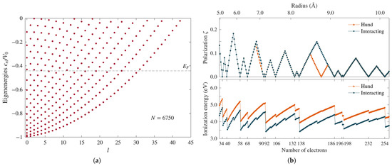
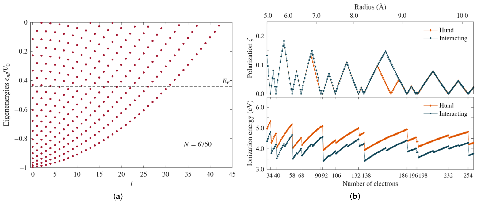
We present in Figure 1a the energy spectrum $\left\{{ϵ}_{\nu }^0\right\}$ for a quantum dot containing 6750 electrons, which corresponds to a radius $R=30.10$ Å. To a given quantum number l corresponds a series of increasing eigenenergies indexed by n, which give rise to the parabola-like substructure of the spectrum. Because of the spherical symmetry, the eigenenergies are independent of the quantum number m, which naturally takes the values $m=-l, -l+1, \dots , l-1, l$. The potential well depth for this dot is 10.01 eV. The energy of the highest occupied states is $E_F=-4.426$ eV and corresponds to states ${\varphi }_{n=2,l=26,m}$. This value is close to the work function value of gold, as one might expect. There is one point on the electronic structure that is worth emphasizing. In our model, all the states arise from the same uniform background and the same boundary conditions at the surface–vacuum interface. Thus, it does not really admit a meaningful characterization of states as being either bulk or surface. States that in experiment arise genuinely from a different environment at the surface are absent in our model.

Figure 1. (a) Energy spectrum ${ϵ}_{\nu =nlm}^0$ of a gold quantum dot with $N=6750$ ($R\simeq 30.1$ Å). The energies are normalized to the potential well depth (10.11 eV). $E_F=-4.426$ eV is the energy of the highest occupied states. It corresponds to states ${\varphi }_{nlm}$ with $l=26$ and $n=2$ (the eigenenergies are degenerate in m). (b) (upper panel) Predicted polarization by Hund’s rules and the interacting model for dots with N in the range 30–260 (see lower panel). The corresponding dot radii are shown in the upper axis. The polarization is different for certain N values, and the set of “magic numbers” (all shells filled) is different between the two approaches. (lower panel) Ionization energies for the two approaches. The interaction U shifts down the corresponding spectrum. Stability is higher at the magic numbers. Notice, however, that the interacting model captures the relative stability of the half-filled shell cases, something which is not reflected in the Hund’s rules ionization spectrum.

The near degeneracy of some states close to $E_F$ is not relevant if one just applies Hund’s rules to occupy the states. On the other hand, when the interaction U is switched on, there can be an effect on the occupation. Specifically, this can occur when there are partially filled l shells because there will be a shift between the up and down spin states. For instance, before a shell starts to be filled with electrons of the opposite spin, such a shift can cause another shell to be filled with electrons of the same spin. This will be reflected in the polarization. To illustrate this, in Figure 1b’s upper panel, we show the polarization as a function of the number of electrons with N ranging from 30 to 260, with the corresponding radii scale shown in the upper axis. There is a clear divergence in polarization between $N=138$ and $N=186$, where Hund’s rules show a drop to zero polarization at $N=168$, while this is not so in the interacting case. There is also a difference in polarization below $N=90$, but much weaker. Although when looking at the spectra for a wider range of dot radii we found that Hund’s rules and the interacting model generally produce the same polarization, it is important to recognize that the magnitude of the polarization can be quite different in many cases. Furthermore, and importantly, the set of “magic numbers”, which is when all shells are filled, is different in the two models, as shown by the figure. It is worth noting that the polarization decreases with N, i.e., the dots tend to be more paramagnetic. (From the calculation point of view, N is a simpler control parameter than R, which is why we refer to N often.)

Another interesting difference is seen in Figure 1b’s lower panel, which compares the ionization energies. The peaks in the plots indicate, of course, which dots are energetically more stable. Not surprisingly, the most stable states correspond to the predicted magic numbers. (The peak corresponding to $N=168$ in the Hund case is hard to see, but it is there.) Although both results correlate significantly, the interaction model manages to capture the relative stability of the half-filled shells, which Hund’s rules cannot reproduce. Indeed, the smaller peaks for half-filled shells in the interacting case are absent in the Hund plot. This is similar to the relative stability of atoms with half-filled shells, a phenomenon well known to chemists [29].

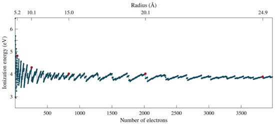
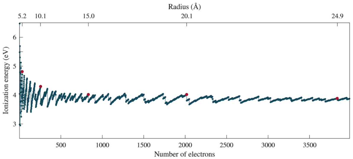
In Figure 2, we look at the ionization energy in a wide range of number of electron values ($N=1,\dots ,3980$). This is to select a number of stable dots to study when we address positron annihilation and Compton scattering. The red dots in the figure indicate stable quantum dots, specifically with $N=34, 254, 832, 2018$, and 3836. The corresponding radii are indicated in the upper axis. In the studies below, we also included a quantum dot with $N=6750$ ($R=30.10$ Å) because it helps see some effects more clearly. For simplicity, when referring to the radii of these dots, hereafter we will use the labels $R=5, 10, 15, 20, 25$, and 30. Note that these dots are maximally stable, meaning all shells are filled and present a polarization $\zeta =0$.

Figure 2. Ionization energies as predicted by the interacting model for dots with $N=1, \dots , 3980$. The red dots in the figure indicate the cases selected for closer study, all maximally stable cases, i.e., with all shells filled. N is such that the radii are close to $R=5, 10, 15, 20$ and 25 Å; see the upper axis scale. The case $N=6750$ ($R\simeq 30$ Å) was further included in the study.

We point our here the following. We expect our model to give an approximate description of the electronic properties of nanoparticles. However, for very small particles, such as those with $R=5$, the approximation is too strong. For instance, it is known that at a small size, the role of d-band electrons becomes increasingly important, and not only for optical properties, catalytic reactivity can also be affected [30]. The ionic character of the positive background is also absent. However, we consider it useful to include small sizes in the study for the purpose of better identifying the trends predicted by our model, as it is mainly its qualitative capabilities we would like to recognize.

3.2. Momentum Density

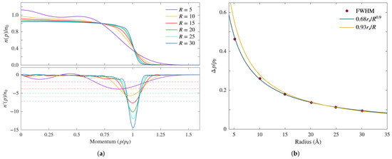
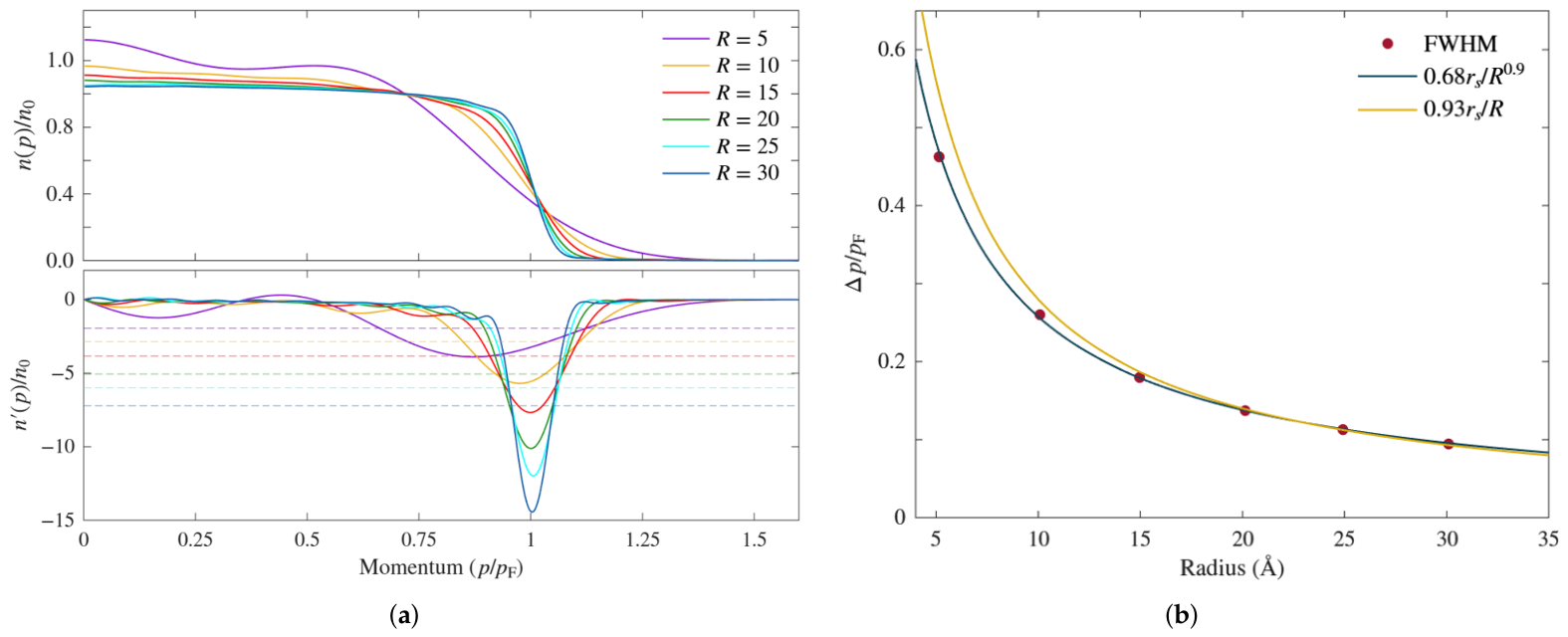
In Figure 3a’s upper panel, we show the momentum density for all six cases considered in the study as predicted by the interacting model at $T=0$. Momentum is normalized to the free electron gas Fermi momentum value for $r_s=3.01$ (i.e., corresponding to gold), which we denote $p_F$. Thus, as in [17], the larger the radius, the more the density tends toward a bulk momentum density. In particular, the momentum decrease around $p_F$ becomes sharper with increasing radius, i.e., the “momentum broadening” as it is referred to by experimentalists, becomes narrower. Note that in the case of $R=5$, there is no well-defined Fermi momentum above which the states would be unoccupied. This is because at that size, the electrons are not behaving as an electron gas. On the other hand, the appearance of a better-defined Fermi momentum for the larger radii indicates that the system is behaving as expected, i.e., like a metal, instead of a giant atom.

Figure 3. (a) (upper panel) Momentum density for the selected dots indicated in Figure 2. With an increasing radius, the momentum density tends toward that of the bulk metal, which presents a sharp momentum density drop around the Fermi momentum $p_F$. The slower decay of the momentum density around $p_F$ is referred to as the “momentum broadening”. (lower panel) The derivative of the momentum density provides a means to quantify the momentum broadening by extracting the full width at half minimum (FWHM) of $n^{\prime }\left(p\right)$. The half-minimum values corresponding to each radius are indicated by the dashed lines. (b) Plot of the calculated FWHM values as a function of the radius, compared with curve fits decaying as $1/R$ and $1/R^{0.9}$. The momentum broadening decay with the radius is subject to experimental study, such as via 2D-ACAR [31].

One way to assess quantitatively the extent of the broadening is to consider the full width at half minimum (FWHM) of the derivative of the momentum density $n^{\prime }\left(p\right)$ [14,17]. The derivatives are shown in Figure 3a’s lower panel, and for each dot radius, there is a corresponding horizontal dashed line indicating the value at half minimum. The strong decrease in the FWHM with the radius is evident. The decreasing behavior is better illustrated in Figure 3b. In [17], it was proposed that $\Delta p$ follows the inverse law $0.93r_s/R$ as a function of the radius. In the present case, that decay is too strong, as shown by the corresponding curve in comparison with the calculated FWHM values (red dots). The deviation from the calculated values increases for $R\lesssim 15$ Å and also for large radii ($R>30$ Å). We find that the present case is more closely fit by the expression $0.68r_s/R^{0.9}$. The decay of the momentum broadening with the radius has been observed experimentally [11,31] and shows approximately a $1/R$ behavior. It is not clear, however, how significant the difference in decay behavior in the figure is from the point of view of experimental accuracy. The difference between the two approximations for the smallest dot, i.e., for $R=5$, is $\sim 0.095$ Å⁻¹. For $R=10$, the difference falls below ∼0.03 Å⁻¹, and is gradually smaller for higher radii. For comparison, the reported momentum resolution in the positron two-dimensional angular correlation of annihilation radiation (2D-ACAR) experiments is $\sim 0.2$ Å⁻¹ [12]. Thus, it would be insufficient to detect such small differences. High-resolution X-ray Compton scattering experiments, on the other hand, present a momentum resolution of ∼0.06 Å⁻¹ [14]. Though significantly higher, the resolution would still not be enough to differentiate between the two approximations at the higher radii values.

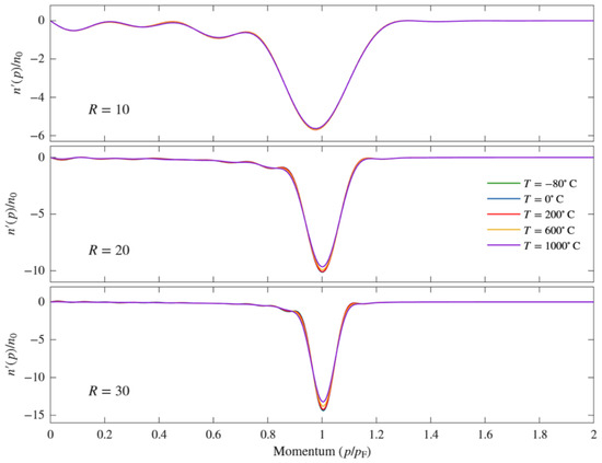
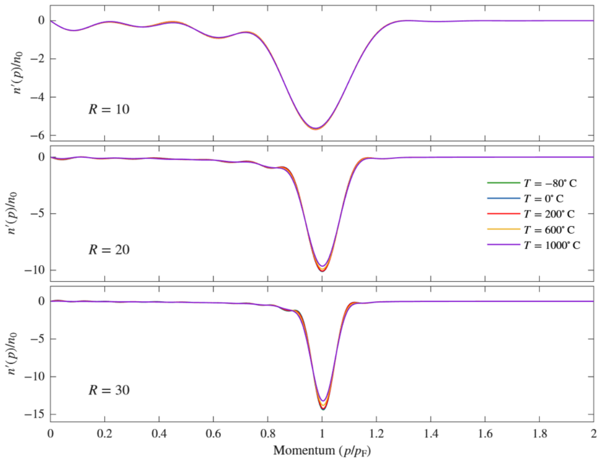
We turn now to the question of the effect of temperature on the momentum density broadening. As indicated in the Introduction, we considered a range of temperatures spanning from $-80$ °C to 1000 °C. We present here the results for five different temperatures, namely $-80$, 0, 200, 600, and 1000 °C, as they are sufficient to show the tendency and magnitude of the effects. We first point out that we find a negligible effect in small dots. This could be expected from their energy spectrum. For instance, in the case of $N=34$ ($R=5.2$ Å), the difference in energy between $E_F$ and the lowest unoccupied level is 1.14 eV, which is enormous even for a temperature of 1000 °C (roughly 0.11 eV). Of course, it could just be circumstantial that there is no accidental energy degeneracy with other energy levels. Nevertheless, we found that, in general, at a low radius, the differences in energy levels are such that the temperature’s effects are not significant. At around $R=10$ Å, the effect begins to be perceptible more systematically. To show the tendency with increasing radius, in Figure 4, we show the momentum density derivatives at the temperatures mentioned above for the dots labeled $R=10$, $R=20$, and $R=30$. The effect is clearly more visible for the larger dot, for which the different effect of the different temperatures is also discernible. We did not plot horizontal lines for the half-minimum values in this case because they would be difficult to distinguish.

Figure 4. Derivatives of the momentum density for $R=10, 20$, and 30 at the temperatures indicated to the right of the panels. The effects are clearly more visible for the larger radii and stronger around the Fermi momentum.

For a more quantitative assessment, we calculated the FWHM values for all the cases considered, and we present them in Table 1. For comparison, the results for $T=0$ K are also included. The last line in the table shows the percentage change between the largest and smallest value for each R. As suggested by Figure 4, the largest percentage change with the temperature corresponds to $R=30$. Notice, however, that the change is higher for $R=20$ than for $R=25$. We think this is an effect of the number of accidental degeneracies or near degeneracies present. How many of these will be present and how close in energy they will be for a dot with a given radius is difficult to predict, and their effect on broadening will depend on the temperature. Notice also that the FWHM is given as a fraction of $p_F$, which is $1.2049$ Å⁻¹. Thus, the largest FWHM percentage change with the temperature in the table ($R=30$) amounts to ∼0.012 Å⁻¹. Unfortunately, this again falls below what is achievable with high-momentum resolution X-ray Compton scattering [14], which is around 0.06 Å⁻¹, as indicated above. Thus, such small temperature effects on momentum broadening currently appear not to be measurable.

Table 1. FWHM values calculated at the temperatures indicated for all six dot sizes selected for this study. The last line shows the FWHM percentage change between the largest and smallest value for each radius. Temperatures are in °C unless otherwise indicated.

T	5	10	15	20	25	30
0 K	0.4625	0.2600	0.1800	0.1375	0.1125	0.0950
−80	0.4625	0.2600	0.1800	0.1350	0.1125	0.0950
0	0.4625	0.2600	0.1800	0.1350	0.1125	0.0925
200	0.4625	0.2600	0.1800	0.1350	0.1150	0.0950
600	0.4625	0.2625	0.1825	0.1400	0.1175	0.0950
1000	0.4625	0.2650	0.1850	0.1425	0.1175	0.1025
%	0	1.9	2.8	5.6	4.4	10.8

3.3. Compton Scattering

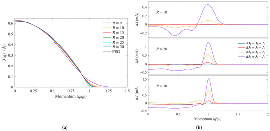
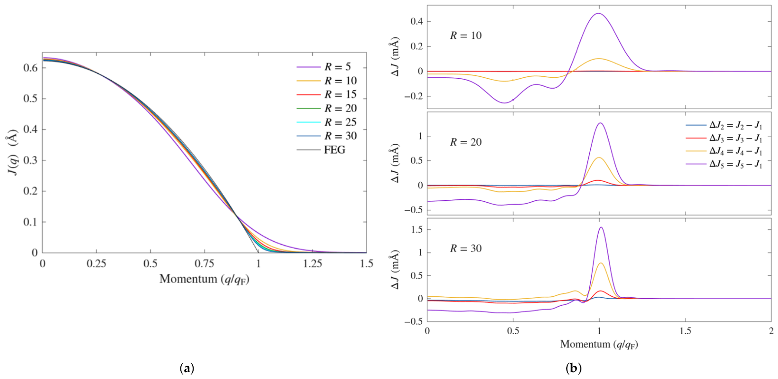
Because of the spherical symmetry in the cases considered (we focused on closed-shell cases, as mentioned before), the Compton profiles depend only on the magnitude of the scattering vector and not on its direction. Thus, $J\left(\mathbf{q}\right)=J\left(q\right)$ in the present case. In Figure 5a, we show the Compton profiles at $T=0$ K for all six dot radii studied compared with the profile for the free electron gas of a density $r_s=3.01$, with the scattering momentum normalized to the corresponding Fermi momentum, which we denote here $q_F$. We recall that (per electron) the profile for the free electron gas is given by the expression [32]

$$J^{\mathrm{FEG}}\left(q\right)={\displaystyle \frac{3}{4q_F}}\left[1-{\displaystyle \frac{q^2}{q_F^2}}\right].$$

(11)

We see that the difference with respect to the FEG profile is stronger for small radii. As already shown by the momentum density plots in Figure 3a, small dots behave more like large molecules, and only at larger dot radii does a bulk-like behavior appear. The deviation from the free electron gas result is stronger above $q_F$ in all cases. The curves are quite similar to the experimental Compton profiles of good metals such as Na and Al [33,34]. The FEG profile is parabolic because it corresponds to the area of a slice of the Fermi sphere at a distance q from the origin. But in a quantum dot, the momentum density varies, and the profile is not just proportional to such an area. In fact, one can have an idea of how the Compton profile will behave qualitatively by looking at the momentum density. For instance, the momentum density for $R=5$ in Figure 3a tells us that below the Fermi momentum, the dot profile will tend to fall below the FEG profile, and that above the Fermi momentum, it will have a non-zero tail.

Figure 5. (a) Compton profiles at $T=0$ K for the six radii indicated compared with that of the free electron gas of a density corresponding to gold (labeled FEG). As one can expect, the profiles approach the FEG profile as the radius increased. (b) Differences between the profiles at higher temperatures and the profile at $T=-80$ °C. $J_1$ stands for the profile at that temperature. $J_2, J_3, J_4$, and $J_5$ stand for the profiles at temperatures $T=0, 200, 600$, and 1000 °C, respectively. The differences $\Delta J$ are labeled accordingly. The results are for the cases $R=10$, 20, and 30 as indicated. The structure in the plots indicates that the weight of the contribution of the different orbitals changes with the temperature and changes more strongly near the Fermi momentum.

We now consider the temperature effects on the Compton scattering spectra. Let us remember that the effects considered here concern changes in state occupation with temperature, with no change in the nature of the nanoparticle or its eigenstates. Compton scattering can be used to detect electronic structure changes with temperature that reflect a phase transition, in which case changes in the spectra can be quite distinct [35]. Here, the temperature effects on the Compton profiles are extremely small even for the larger radii, and thus a direct comparison of the profiles for the different temperatures would not give much information. To better illustrate the effect of temperature, we considered the difference $\Delta J$ between the profiles at temperatures $T=0, 200, 600$, and 1000 °C and the profile at $T=-80$ °C. For simplicity, we label the profiles for the former temperatures $J_2, J_3, J_4$, and $J_5$, respectively, and $J_1$ for the latter. In Figure 5b, we present the results for the dots of radii 10, 20, and 30 Å as indicated in the different panels, with the colors having the same meaning for all three. The structure in the plots reflects the change in weight of the contribution of the different orbitals due to temperature, showing a stronger effect near $q_{\mathrm{F}}$. Now, Ohata et al. have measured differences of 1% between profiles along different directions in Al [34]. In this perspective, and to attempt to make contact with the experiment, we calculated the percent differences aat $q=0$ and $q=q_{\mathrm{F}}$ for the three cases in Figure 5b. The results are shown in Table 2. As can be seen, the percent differences at $q=0$ are either completely negligible or fall well below 1%, unfortunately. Nevertheless, we show the results for completeness. As could perhaps be expected from Figure 5b, at $q=q_{\mathrm{F}}$, the situation is much better, with differences of several percent in some cases. Thus, the difference is, in principle, measurable in those cases. We add that since in [34] a statistical uncertainty below 0.3% (per datum) and a momentum resolution of 0.12 a.u. are indicated, it is possible that differences of a fraction of 1% can still be measured, especially if a momentum resolution of $\sim 0.03$ a.u. can be used, as in the experiments of Hiraoka et al. [14].

Table 2. Percent changes at $q=0$ and $q=q_{\mathrm{F}}$ of the profile differences plotted in Figure 5b. The percent changes at $q=0$ appear to be generally negligible and are shown for completeness. At $q=q_{\mathrm{F}}$, however, at a higher radius and temperature, the changes fall well within the current experimental resolution (see Discussion in the main text).

		$q=0$			$q=q_F$
$\Delta J/J_1$	$R=10$	$R=20$	$R=30$	$R=10$	$R=20$	$R=30$
$\Delta J_2/J_1$	0	0	$-0.01$	0	0.04	0.13
$\Delta J_3/J_1$	0	0	$-0.01$	$0.01$	0.33	0.67
$\Delta J_4/J_1$	0	$-0.01$	$0.01$	$0.22$	1.82	3.09
$\Delta J_5/J_1$	$-0.01$	$-0.05$	$-0.04$	1.01	4.04	6.11

Let us comment on why atomic vibrations can be neglected. In Compton scattering, X-rays are used, with energies to the order of keV [14]. Thus, the photon scattering momenta are immense compared to any phonon or vibrational momenta. Also, scattering times are of the order of $\sim {10}^{-18}$ s [36], which is much shorter than typical phonon periods. Indeed, in gold, the Debye temperature is 170 K [25], which corresponds to $\sim 2.8\times {10}^{-13}$ s. The minor effect that nuclei dynamics has on Compton profiles has indeed been verified experimentally in highly accurate synchrotron-based Compton scattering studies on ice Ih [37]. On the other hand, the temperature could have an indirect effect on Compton profiles at radii of interest to plasmonics. Indeed, research has shown that because of thermal expansion, there is an increasing red shift and broadening of the surface plasmon resonance in gold nanoparticles as the temperature increases from 17 °C to 915 °C [38]. It is possible that the underlying changes in the electronic structure can be detected in Compton scattering experiments.

3.4. Positron Lifetime

For reference, the positron annihilation rate in a homogeneous electron gas (HEG) of density $r_s$ is given by $\lambda =3r_e^{2}c\gamma /4r_s^3\approxeq 12\gamma /r_s^3$ (ns⁻¹), with $\gamma$ given by Equation (6) [23]. For gold, the lifetime is then $\tau =1/\lambda =265.0$ ps. We calculated the positron lifetimes at the four finite temperatures discussed above as well as the lifetime at $T=0$ for all six dot radii studied above. The results are shown in Table 3, where the lifetimes are in ps. Although the LDA enhancement factor tends to underestimate the lifetimes, we included the corresponding results in the table for completeness.

Table 3. Calculated positron lifetimes (ps) for the selected temperatures and dot sizes considered in this work. The two enhancement factors discussed in the main text were considered. The LDA enhancement factor typically underestimates lifetimes, which is corroborated here. For reference, the positron lifetime in the HEG of density $r_s=3.01$ is 265.0 ps. Temperatures are in °C unless otherwise indicated.

$\mathit{\gamma }$	T	5	10	15	20	25	30
	0 K	439.2	267.7	260.0	261.0	259.9	261.6
GCA	−80	439.2	267.7	260.0	261.0	260.0	261.3
	0	439.2	267.7	260.0	261.0	260.1	261.2
	200	439.2	267.7	260.2	260.9	260.4	261.1
	600	439.1	267.7	260.6	260.7	260.7	261.2
	1000	439.0	267.5	260.9	260.7	260.9	261.3
	0 K	316.7	261.2	258.2	260.2	259.5	261.4
LDA	−80	316.7	261.2	258.2	260.2	259.6	261.1
	0	316.7	261.2	258.2	260.2	259.7	261.0
	200	316.7	261.2	258.3	260.1	260.0	260.9
	600	316.7	261.1	258.7	259.9	260.3	261.0
	1000	316.6	261.0	259.1	260.0	260.5	261.1

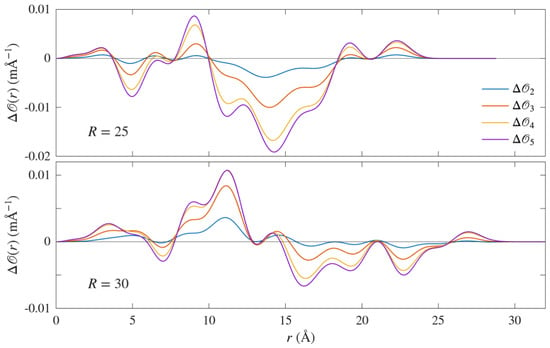
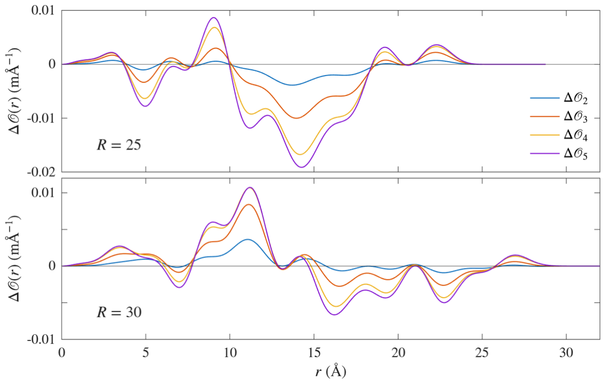
We note first that the lifetimes at $T=-80$ °C are basically the same as for $T=0$ K, except for the larger dots. (The lifetimes at $T=0$ K obtained in Ref. [17] are quite generally lower than what we obtain here. The main reason can be traced back to the different quantum well depth used in that work, which does not take into account the size dependence of the work functions.) Lifetimes at $T=-80$ °C do not depart noticeably from those at $T=0$ K because the Fermi–Dirac occupation smearing is rather narrow at that temperature. The energy spectrum of the larger dots is much denser, and thus they show a temperature effect. Second, there is a rather large drop in the lifetime when considering dot radii above $R=5$. The lifetime in the latter case is markedly higher because the positron state is shallow in that case, i.e., it is weakly bound, and its density spills out of the dot well much more than the electron density. Thus, overlap between the two is considerably reduced, and the annihilation rate is lower [we verified that below $N=20$ ($R\simeq 4.32$ Å), there are no more positron bound states in the dot]. For increasing dot sizes, the positron density gradually falls entirely within the dot, and thus it overlaps with the electron density more fully, increasing the annihilation rate. Thus, lifetimes decrease noticeably up to $R=15$ but change only weakly above that radius. Third, lifetime changes with the temperature are small, and part of the reason the data in the Table are given up to a fraction of a picosecond is to try to identify some trend. Note that those differences are below the resolution reported in experiment [13,39,40], where the error bars are typically to the order of a few picoseconds. There appears to be no common trend. Lifetimes tend to decrease slightly with the temperature for $R=5,10$, and 20, and they tend to increase for $R=15$ and 25. For $R=30$, they first decrease and then increase. Nevertheless, we attribute the decreasing or increasing behavior to small changes with temperature of the overlap of the positron and electron densities. To illustrate this, we considered change with the temperature of the annihilation rate amplitude $\mathcal{O}\left(r\right)=r^{2}n\left(r\right)n_{+}\left(r\right)$ [see Equation (5) (we omit $\gamma$, see below)] for the cases $R=25$ and $R=30$. Similar to the labeling in the case of the Compton profiles, we used the labels ${\mathcal{O}}_1, \dots , {\mathcal{O}}_5$ for the probability amplitudes of $T= -80, 0, 200, 600$, and 1000 °C, respectively. Taking as reference ${\mathcal{O}}_1$, we denote $\Delta {\mathcal{O}}_2={\mathcal{O}}_2-{\mathcal{O}}_1$, and $\Delta {\mathcal{O}}_3, \Delta {\mathcal{O}}_4$, and $\Delta {\mathcal{O}}_5$ have the corresponding meaning. The results are plotted in Figure 6. We can see why lifetimes increase in the case of $R=25$: $\Delta \mathcal{O}$, mainly decreases with the temperature, i.e., the annihilation rate decreases. The results for $R=30$ can be understood in a similar way; ${\mathcal{O}}_2$ is, on average, larger for ${\mathcal{O}}_1$ (i.e., increased annihilation rate), while at the other end, the difference between ${\mathcal{O}}_5$ and ${\mathcal{O}}_1$ basically cancels out. We point out that we do not include the enhancement factor $\gamma$ in the definition of $\mathcal{O}$ to demonstrate the leading role of the overlap of the densities [$\gamma$ is essentially flat up to when r is close to R (in both the LDA and GGA cases).

Figure 6. Changes of the annihilation rate amplitude with temperature. We denote ${\mathcal{O}}_1, \dots , {\mathcal{O}}_5$ the annihilation rate amplitudes at $T=-80, 0, 200, 600$, and 1000 °C, respectively. In the plots $\Delta {\mathcal{O}}_i={\mathcal{O}}_i-{\mathcal{O}}_1$, for i = 2, 3, 4, 5, i.e., the annihilation rate amplitude at $T=-80$ °C is taken as reference. In the case of $R=25$ the difference tends to increase with temperature. In the case of $R=30$, on the other hand, the difference first increases, to later decrease and cancel out as temperature increases.

It is important to point out the following. In experiment, lifetimes can have several components, with different values for positrons trapped in the nanoparticle and those trapped at the surface (see, for instance, [39]). Our model only considers the first case. To simulate trapping at the surface, we would have to include in our Hamiltonian an image-like potential at the surface of the dot. Thus, that case is outside the scope of the present work. Let us end on a comment on the neglect of ionic thermal effects. In positron annihilation, positrons interact mainly with electrons with energies around the Fermi level. Thus, the momenta involved in the scattering are much larger than the moment that could be associated with atomic vibrations and therefore can be reasonably neglected, as in the case of Compton scattering. We also considered the possible effect of thermal expansion. For this, we relied on the volume expansion coefficient for gold nanoparticles as parametrized in [38], where the temperature dependence of the coefficient itself is also taken into account. The largest change we found was at $T=1000$ °C and for $R=5$ in the GGA case, for which the difference with the result in Table 3 was 7.2 ps. This should be measurable, as the resolution in the experiment is to the order of a few picoseconds, as discussed above. Unfortunately, $R=5$ is the least realistic case, and in the other cases, the difference at that temperature reduces to around 3 ps. At lower temperatures, the difference rapidly falls to lower values. For instance, at $T=200$ °C, the difference for $R=5$ is 1.2 ps, while for the other radii, it is 0.5 ps. Thus, in this case, the changes are generally predicted to be from borderline to below experimental resolution.

4. Conclusions

In this work, we use a quantum dot model, a Hamiltonian, and a Hubbard-like effective electron–electron interaction to study temperature effects on the electronic properties of dots of various sizes. For this, we use the finite-temperature Green function formalism. The quantum dot model as well as the Hamiltonian were improved with respect to previous work, namely size effects are taken into account to determine the dot potential well depth, and the Coulomb U parameter value taken for the interaction has a more sound basis. The main differences that this brings with respect to previous work are that the momentum broadening decay with the dot radius is slower, and the positron lifetimes are generally higher. With regard to temperature effects, which were not studied before, we found that they were small. This goes as well for the momentum density broadening as for the Compton profiles and the positron lifetimes. We found that the value of the relevant quantities are rather stable in the temperature range between $-80$ °C and $1000$ °C. One can assume that this stability may be part of the reason why gold nanoparticles are used in the wide range of temperatures mentioned in the Introduction. Of course, the present study is limited to temperature effects, and it does not address other experimental conditions, such as chemical or molecular environments. Future work on temperatures effects could be oriented toward a more realistic description of the underlying electronic system, including a surface potential, possibly based on first-principles methods.

References

- Bell, A.T. The impact of nanoscience on heterogeneous catalysis. Science 2003, 299, 1688. [Google Scholar] [CrossRef] [Scilit] [PubMed]
- Joudeh, N.; Linke, D. Nanoparticle classification, physicochemical properties, characterization, and applications: A comprehensive review for biologists. J. Biotechnol. 2022, 20, 262. [Google Scholar] [CrossRef] [Scilit] [PubMed]
- Ma, Z.; Yin, H.; Overbury, S.H.; Dai, S. Metal phosphates as a new class of supports for gold nanocatalysts. Catal. Lett. 2008, 126, 20–30. [Google Scholar] [CrossRef] [Scilit]
- An, A.-F.; Lu, A.-H.; Sun, Q.; Wang, J.; Li, W.-C. Gold nanoparticles stabilized by a flake-like Al2O3 support. Gold. Bull. 2011, 44, 217–222. [Google Scholar] [CrossRef] [Scilit]
- Liu, S.S.; Xu, W.; Niu, Y.; Zhang, B.; Zheng, L.; Liu, W.; Li, L.; Wang, J. Ultrastable Au nanoparticles on titania through an encapsulation strategy under oxidative atmosphere. Nat. Commun. 2019, 10, 5790. [Google Scholar] [CrossRef] [Scilit] [PubMed]
- Mishra, A.; Shaikh, S.; Kumar, A. Progressive cryoaggregation of gold nanoparticles: Physiochemical characterization, effect on biological interactions and use in coldness indicators. Colloid. Surf. A 2022, 636, 128158. [Google Scholar] [CrossRef] [Scilit]
- Yukhta, M.; Bespalova, I.; Koroleva, A.; Chichkov, B. Nanoparticles in low-temperature preservation of biological systems of animal origin. Nanotechnol. Rev. 2025, 14, 20250143. [Google Scholar] [CrossRef] [Scilit]
- Manson, J.; Kumar, D.; Meenan, B.J.; Dixon, D. Polyethylene glycol functionalized gold nanoparticles: The influence of capping density on stability in various media. Gold. Bull. 2011, 44, 99–105. [Google Scholar] [CrossRef] [Scilit]
- Her, S.; Jaffray, D.A.; Allen, C. Gold nanoparticles for applications in cancer radiotherapy: Mechanisms and recent advancements. Adv. Drug Deliv. Rev. 2017, 109, 84–101. [Google Scholar] [CrossRef] [Scilit] [PubMed]
- Eijt, S.W.H.; Van Heen, A.; Schut, H.; Mijnarends, P.E.; Denison, A.B.; Barbiellini, B.; Bansil, A. Study of colloidal quantum-dot surfaces using an innovative thin-film positron 2D-ACAR method. Nat. Mater. 2016, 5, 23–26. [Google Scholar]
- Eijt, S.W.H.; Barbiellini, B.; Houtepen, A.J.; Vanmaekelbergh, D.; Mijnarends, P.E.; Bansil, A. Positron studies of surfaces, structure and electronic properties of nanocrystals. Phys. Stat. Sol. (C) 2007, 4, 3883–3888. [Google Scholar] [CrossRef] [Scilit]
- Toyama, T.; Tang, Z.; Inoue, K.; Chiba, T.; Ohkubo, T.; Hono, K.; Nagai, Y.; Hasegawa, M. Size estimation of embedded Cu nanoprecipitates in Fe by using affinitively trapped positrons. Phys. Rev. B 2012, 86, 104106. [Google Scholar] [CrossRef] [Scilit]
- Chai, L.; Al-Sawai, W.; Gao, Y.; Houtepen, A.J.; Mijnarends, P.E.; Barbiellini, B.; Schut, H.; van Schaarenburg, L.C.; van Huis, M.A.; Ravelli, L.; et al. Surfaces of colloidal PbSe nanocrystals probed by thin-film positron annihilation spectroscopy. APL Mater. 2013, 1, 022111. [Google Scholar] [CrossRef] [Scilit]
- Hiraoka, N.; Nomura, T. Electron momentum densities near Dirac cones: Anisotropic Umklapp scattering and momentum broadening. Sci. Rep. 2017, 7, 565. [Google Scholar] [CrossRef] [Scilit] [PubMed]
- Feng, Z.; Zhang, X.; Sakurai, Y.; Wang, Z.; Li, H.; Hu, H. Compton profile of few-layer graphene investigated by electron energy-loss spectroscopy. Sci. Rep. 2019, 9, 17313. [Google Scholar] [CrossRef] [Scilit] [PubMed]
- Caputo, R.; Fukazawa, Y.; Johnson, R.P.; Longo, F.; Prest, M.; Tajima, H.; Vallazza, E. Silicon detectors for gamma-ray astronomy. In Handbook of X-Ray and Gamma-Ray Astrophysics; Bambi, C., Santangelo, A., Eds.; Springer Nature: Singapore, 2024; pp. 1969–1997. [Google Scholar]
- Saniz, R.; Barbiellini, B.; Denison, A. Compton scattering, positron annihilation, and the electronic properties of quantum dots. Phys. Rev. B 2002, 65, 245310. [Google Scholar] [CrossRef] [Scilit][Green Version]
- Saniz, R.; Barbiellini, B.; Denison, A.B.; Bansil, A. Spontaneous magnetization and electron momentum density in three-dimensional quantum dots. Phys. Rev. B 2003, 68, 165326. [Google Scholar] [CrossRef] [Scilit][Green Version]
- Amendola, V.; Pilot, R.; Frasconi, M.; Maragò, O.M.; Iati, M.A. Surface plasmon resonance in gold nanoparticles: A review. J. Phys. Condens. Matter 2017, 29, 203002. [Google Scholar] [CrossRef] [Scilit] [PubMed]
- Bansil, A.; Nissenbaum, D.; Barbiellini, B.; Saniz, R. Electron correlations, spontaneous magnetization and momentum density in quantum dots. J. Phys. Chem. Solids 2004, 65, 2005–2009. [Google Scholar] [CrossRef] [Scilit][Green Version]
- Dugdale, S.B. Probing the Fermi surface by positron annihilation and Compton scattering. Low. Temp. Phys. 2014, 40, 328–338. [Google Scholar] [CrossRef] [Scilit]
- Mahan, G.D. Many-Particle Physics, 1st ed.; Plenum Press: New York, NY, USA, 1981. [Google Scholar]
- Barbiellini, B. Positron studies in materials: DFT and QMC studies. In New Directions in Antimatter Chemistry and Physics; Surko, C.M., Gianturco, F.A., Eds.; Kluwer Academic Publishers: Dordrecht, The Netherlands, 2001; pp. 1–24. [Google Scholar]
- Ishibashi, S.; Tokumoto, M.; Kinoshita, N.; Terada, N.; Ihara, H.; Suzuki, R.; Ohdaira, T.; Mikado, T.; Anzai, H. Positron lifetimes in molecular crystals. Can. J. Phys. 1996, 74, 534–539. [Google Scholar] [CrossRef] [Scilit]
- Ashcroft, N.W.; Mermin, N.D. Solid State Physics, 1st ed.; Saunders College: Rochester, NY, USA, 1976. [Google Scholar]
- Wood, D.M. Classical size dependence of the work function of small metallic spheres. Phys. Rev. Lett. 1981, 46, 749. [Google Scholar] [CrossRef] [Scilit]
- Vosko, S.H.; Wilk, L.; Nusair, M. Accurate spin-dependent electron liquid correlation energies for local spin density calculations: A critical analysis. Can. J. Phys. 1980, 58, 1200–1211. [Google Scholar] [CrossRef] [Scilit]
- Pikart, P.; Hugenschmidt, C.; Horisberger, M.; Matsukawa, Y.; Hatakeyama, M.; Toyama, T.; Nagai, Y. Positron annihilation in Cr, Cu, and Au layers embedded in Al and quantum confinement of positrons in Au clusters. Phys. Rev. B 2011, 84, 014106. [Google Scholar] [CrossRef] [Scilit]
- Atkins, P.; de Paula, J.; Keeler, J. Physical Chemistry, 11th ed.; Oxford University Press: Oxford, UK, 1918. [Google Scholar]
- van Bokhoven, J.A.; Miller, J.T. D Electron density and reactivity of the d band as a function of particle size in supported gold catalysts. J. Phys. Chem. C 2007, 111, 9245–9249. [Google Scholar] [CrossRef] [Scilit]
- Chiba, T.; Nagai, Y.; Tang, Z.; Akahane, T.; Hasegawa, M.; Takenaka, M.; Kuramoto, E. Electronic structure of nanosized bcc Cu precipitates in Fe-Cu alloys studied by positron 2D-ACAR. Mater. Sci. Forum 2004, 445–446, 3980. [Google Scholar] [CrossRef] [Scilit]
- Aguiar, J.C.; Mitnik, D.; Di Rocco, H.O. Electron momentum density and Compton profile by a semi-empirical approach. J. Phys. Chem. Solids 2015, 83, 64–69. [Google Scholar] [CrossRef] [Scilit]
- Dugdale, S.B.; Jarlborg, T. Thermal disorder versus correlation in Compton profiles from alkali metals. Solid State Commun. 1998, 105, 283–287. [Google Scholar] [CrossRef] [Scilit]
- Ohata, T.; Itou, M.; Matsumoto, I.; Sakurai, Y.; Kawata, H.; Shiotani, N.; Kaprzyk, S.; Mijnarends, P.E.; Bansil, A. High-resolution Compton scattering study of the electron momentum density in Al. Phys. Rev. B 2000, 62, 16528–16535. [Google Scholar] [CrossRef] [Scilit]
- Koizumi, A.; Motoyama, G.; Kubo, Y.; Tanaka, T.; Itou, M.; Sakurai, Y. f Electron contribution to the change of electronic structure in CeRu2Si2 with Temperature: A Compton Scattering Study. Phys. Rev. Lett. 2011, 106, 136401. [Google Scholar] [CrossRef] [Scilit] [PubMed]
- Chatzidimitriou-Dreismann, C.A.; Vos, M.; Kleiner, C.; Abdul-Redah, T. Comparison of electron and neutron Compton scattering from entangled protons in a solid polymer. Phys. Rev. Lett. 2003, 91, 057403. [Google Scholar] [CrossRef] [Scilit] [PubMed]
- Nygøard, K.; Hakala, M.; Manninen, S.; Itou, M.; Sakurai, Y.; Haämäläinen, K. Configurational energetics in ice Ih probed by 500 Compton scattering. Phys. Rev. Lett. 2007, 99, 197401. [Google Scholar] [CrossRef] [Scilit] [PubMed]
- Yeshchenko, O.A.; Bondarchuk, L.S.; Gurin, V.S.; Dmitruk, I.M.; Kotko, A.V. Temperature dependence of the surface plasmon resonance in gold nanoparticles. Surf. Sci. 2013, 608, 275–281. [Google Scholar] [CrossRef] [Scilit]
- Shi, W.; Callewaert, V.; Barbiellini, B.; Saniz, R.; Butterling, M.; Egger, W.; Dickmann, M.; Hugenschmidt, C.; Shakeri, B.; Meulenberg, R.W.; et al. Nature of the positron state in CdSe quantum dots. Phys. Rev. Lett. 2018, 121, 057401. [Google Scholar] [CrossRef] [Scilit] [PubMed]
- Nokelainen, J.; Barbiellini, B.; Kuriplach, J.; Eijt, S.; Ferragut, R.; Li, X.; Kothalawala, V.; Suzuki, K.; Sakurai, H.; Hafiz, H.; et al. Identifying redox orbitals and defects in lithium-ion cathodes with Compton scattering and positron annihilation spectroscopies: A review. Condens. Matter 2022, 7, 47. [Google Scholar] [CrossRef] [Scilit]
Disclaimer/Publisher’s Note: The statements, opinions and data contained in all publications are solely those of the individual author(s) and contributor(s) and not of MDPI and/or the editor(s). MDPI and/or the editor(s) disclaim responsibility for any injury to people or property resulting from any ideas, methods, instructions or products referred to in the content. |
© 2026 by the authors. Licensee MDPI, Basel, Switzerland. This article is an open access article distributed under the terms and conditions of the Creative Commons Attribution (CC BY) license.