


Abstract
Fish schooling is a common phenomenon in nature, and offers valuable inspiration for the design of underwater biomimetic propulsors. To investigate the fluid interaction mechanisms among individuals in an oblique tandem arrangement, this study conducts two-dimensional numerical simulations of three airfoil-based biomimetic fish models. Using Computational Fluid Dynamics, the effects of streamwise spacing (–) and orientation angle (–) on the hydrodynamic performance and wake characteristics of each fish are examined for a selected set of five representative cases. The results show that, within the present parameter range, the overall time-averaged thrust coefficient of the three-fish school in an oblique tandem arrangement is higher than that of a single fish, with an increase ranging from 16% to 22%. As the streamwise spacing increases, the mutual interference among individuals weakens, and the overall thrust gain gradually decreases. With increasing orientation angle, the thrust gain of the leading and middle fish decreases, whereas that of the trailing fish transitions from negative to positive. At a small orientation angle (), the leading and middle fish show a substantial thrust increase. This preliminary study indicates that, within the examined parameter space, appropriately adjusting the streamwise spacing and orientation angle can effectively enhance the overall thrust of a fish school in an oblique tandem arrangement and enable the trailing fish to achieve a thrust gain.
Key Contribution:
This study quantifies the effects of streamwise spacing (0.8L–1.2L) and orientation angle (10–30°) on thrust performance as well as wake characteristics of three oblique tandem biomimetic fish. The overall time-averaged thrust coefficient is 16–22% higher than that of a solitary swimmer. Thrust gain decreases with increasing spacing, while the trailing fish’s thrust transitions from negative to positive as orientation angle increases, revealing interactive effects of spacing and angle on thrust benefit.
1. Introduction
Fish are common aquatic animals whose schooling behavior is widespread in nature [1]. Fish school to avoid predators [2] and forage for food [3]. Beyond these ecological advantages, schooling also involves underlying hydrodynamic mechanisms that affect swimming performance—a topic that has long attracted research interest in the fields of biomechanics and biomimetic engineering [4].
Since Gray [5] proposed “Gray’s paradox”, researchers have realized that the swimming efficiency of fish far exceeds the predictions of traditional fluid mechanics models, sparking systematic investigations into the mechanisms of fish locomotion. For example, Lighthill’s slender-body theory [6] first established parametric criteria for the kinematics of efficient swimming in fish. Wu [7] elucidated the mechanical principles underlying undulatory propulsion in fish, laying a theoretical foundation for subsequent studies on fish swimming biomechanics and biomimetic propulsion. Using quantitative flow visualization and electromyography, Liao et al. [8] revealed the hydrodynamic and neuromuscular mechanisms by which fish adopt a low-energy slaloming motion in vortical flows. Xiao et al. [9] employed a moving adaptive mesh method to investigate the interaction between an undulating airfoil and the wake of a D-section cylinder, uncovering a thrust amplification effect and passive drag reduction. Ji et al. [10] applied dynamic mesh techniques to study the energy extraction efficiency of a flexible undulating body, demonstrating its non-monotonic dependence on Reynolds number and wave speed. Their findings provide a theoretical basis for parameter optimization in biomimetic propulsion systems.
As research on the propulsion mechanisms and wake structures of solitary swimmers has matured, the research focus has gradually shifted from individual fish to the complex flow interactions within various schooling configurations [11,12,13,14]. In two-fish systems, Dewey et al. [15] experimentally investigated the interaction between two parallel hydrofoils and found that in-phase undulation enhances propulsive efficiency. Boschitsch et al. [16] conducted experiments on tandem hydrofoils, demonstrating that under optimal spacing and phase difference, the efficiency of the trailing hydrofoil can be significantly improved. Using a space—time finite element method, Dong and Lu [17] studied parallel undulating foils and obtained results consistent with those of Dewey et al. [15]. Khalid et al. [18] employed an immersed-boundary method to simulate two fish swimming in tandem, revealing a nonlinear coupling mechanism in the hydrodynamic forces between the leading and trailing fish, as well as an asymmetric benefit distribution. In multi-fish systems, Deng and Shao [19] used an improved immersed-boundary method to extract a three-fish subunit from a diamond-shaped school and found that the trailing fish can benefit from the reverse von Kármán vortex street shed by the upstream fish. Park and Sung [20] systematically compared the performance of various formations using the immersed-boundary method, showing that individual benefits are closely related to their local position within the school. They reported enhanced overall efficiency in triangular and diamond formations, with more pronounced benefits for trailing individuals. Li et al. [21] compared the swimming efficiency of four biomimetic formations (tandem, phalanx, diamond, and rectangle) at different spacings and identified that the optimal formation for robotic fish swarms depends on the spacing. They further proposed a formation selection strategy based on a critical spacing of 1.25 body lengths. These studies demonstrate that a well-organized schooling configuration can benefit individuals through two key mechanisms: the vortex hypothesis [22] and the channeling effect [23]. Therefore, investigating the fluid interaction mechanisms under different tandem arrangement parameters (streamwise spacing and orientation angle) helps to understand how individuals influence each other during collective swimming.
This study employs the commercial Computational Fluid Dynamics (CFD) software Simcenter STAR-CCM+, based on the finite volume method and the overset mesh technique, to investigate the effects of streamwise spacing and orientation angle on the hydrodynamic performance and wake characteristics of three airfoil-based biomimetic fish models arranged in an oblique tandem manner. The paper is organized as follows. Section 2 describes the numerical methods and physical problem, including the grid and time-step independence verifications. Section 3 presents an analysis of the effects of spacing and orientation angle on each fish in terms of time-averaged force coefficients, force coefficient spectra, and flow field characteristics (wake vortices, velocity, and pressure). Section 4 summarizes the main conclusions of this study.
2. Materials and Methods
2.1. Numerical Methods and Physical Models
Numerical simulations are performed using the commercial CFD software Simcenter STAR-CCM+ (Version 17.04.007). The governing equations are the unsteady incompressible Navier–Stokes equations:
where , are the Cartesian velocity components, p is the pressure, is the fluid density, and is the kinematic viscosity. A laminar flow model was employed. The equations were discretized using the finite volume method. The pressure–velocity coupling was handled via the SIMPLE algorithm. Time advancement was performed using a second-order implicit scheme. An overset mesh technique was adopted to handle the motion of the fish bodies, with the overset interface interpolating the flow variables between the background mesh and the overlapping component meshes.
Two-dimensional numerical simulations are performed on a simplified biomimetic fish model using a National Advisory Committee for Aeronautics (NACA) 0012 airfoil. The use of the NACA 0012 airfoil as a two-dimensional simplified model of a fish body has been widely adopted in bio-inspired hydrodynamics [9,10,17,18]. This simplification provides a geometrically well-defined foil profile that facilitates parametric studies under controlled conditions. The kinematics are set based on the undulatory motion of real fish, ensuring that the essential features of fish-like propulsion are retained. Therefore, employing the NACA 0012 airfoil as the fish model represents a reasonable and effective simplification for the present parametric investigation of hydrodynamic interactions in fish schooling. The kinematic equation along the fish’s centerline is set as:
where y is the lateral coordinate for any position along the fish body at a time-instant t, x is the streamwise coordinate along the fish body, with the origin at the head and the positive direction pointing toward the tail; the positive y-direction is obtained by rotating the positive x-direction by counterclockwise; L is the body length; is the angular frequency; the phase speed is given by ; and is the wave number. The amplitude envelope of the undulatory motion is given by:
The coefficients , , and are determined using the kinematic data of a steadily swimming saithe fish [24]. From these data, the amplitude values , , and are obtained, yielding , , and .
In the present study, all three fish are set to undulate in phase, i.e., the phase difference among them is zero.
The Reynolds number and Strouhal number are two key parameters in fish swimming studies, defined as:
where U is the swimming speed of the fish, is the kinematic viscosity of water, is the tail-beat frequency, and is twice the maximum tail-beat amplitude. In the present simulations, the Strouhal number is fixed at . The Reynolds number is set to , which is lower than the typical values encountered by swimming fish in nature. At this Reynolds number, the flow remains laminar, allowing the core vortex structures generated by the undulating fish body and their evolution to be effectively captured. It is worth noting that this value is consistent with the commonly adopted benchmark in parametric studies of fish schooling hydrodynamics [10,18], where the primary objective is to capture the fundamental vortex interaction mechanisms under controlled, well-resolved laminar conditions. This choice preserves the essential physical characteristics of the wake dynamics and is sufficient for a preliminary investigation of the interaction mechanisms. Extension to higher Reynolds numbers, which would be required for quantitative predictions in under real swimming conditions, is left for future work.
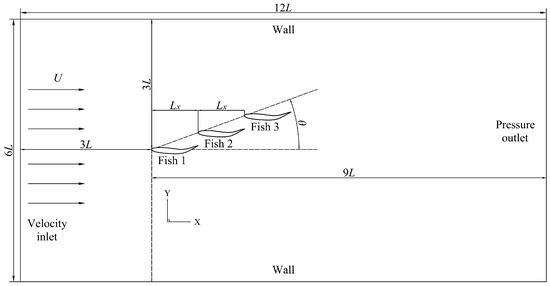
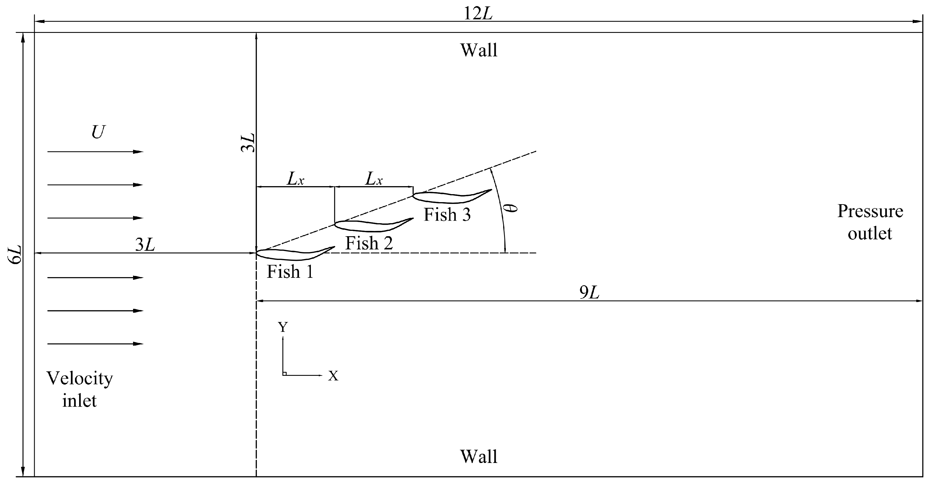
The hydrodynamic performance of three biomimetic fish arranged in an oblique tandem manner is investigated for various streamwise spacings and orientation angles, as illustrated in Figure 1.
Figure 1.
Computational domain and three-fish oblique tandem arrangement.
In Figure 1, Fish1, Fish2, and Fish3 are defined as the front fish, mid fish, and rear fish in the oblique tandem arrangement, respectively. In Figure 1, Fish1, Fish2, and Fish3 are defined as the front fish, mid fish, and rear fish in the oblique tandem arrangement, respectively. The geometric parameters for all cases are summarized in Table 1, where denotes the streamwise spacing (axial gap) between adjacent fish, defined as the horizontal distance from the head of the leading fish to the head of the following fish; is the orientation angle, defined as the angle between the line connecting the heads of the three fish and the positive x-direction; the lateral offset is the perpendicular distance between adjacent fish axes, given by ; the head-to-head distance is the straight-line distance between the heads of adjacent fish, given by /; and the minimum surface-to-surface gap is listed in the “Min.gap” column of Table 1.
Table 1.
Computational cases for the three-fish oblique tandem arrangement, including geometric parameters for all cases.
The selected streamwise spacings are , and the selected orientation angles are . The upper bound of the streamwise spacing is motivated by the finding of Li et al. [21], who reported that the hydrodynamic interaction becomes weak when the spacing exceeds approximately . Thus, the present range up to is expected to capture the transition from noticeable interaction to weak interaction. The lower bound is chosen to avoid physical overlap between adjacent fish bodies, as confirmed by the positive minimum surface-to-surface gaps listed in Table 1 (ranging from to ).
In the present simulations, the biomimetic fish are tethered, and their hydrodynamic performance is characterized by the dimensionless drag and lift coefficients, and , defined as:
where is the fluid density and and are the drag and lift forces, respectively.
In this study, thrust is defined as the force opposite to the incoming flow direction. Thus, when the drag coefficient is negative, its absolute value corresponds to the thrust coefficient, which is expressed as:
To enable a parametric analysis of the thrust performance, a dimensionless time-averaged thrust coefficient is introduced as:
where is the time-averaged thrust coefficient of a biomimetic fish in the school, is that of a solitary fish, and is the dimensionless thrust coefficient, which quantifies the relative change in thrust performance of an individual when swimming in a school compared to solitary swimming. It should be noted that the present analysis focuses on thrust characteristics and wake dynamics. Quantities related to energy performance, including input power, work per cycle, propulsive efficiency, cost of transport, and self-propelled speed, are not evaluated in this study.
In the present simulations, it was observed that a periodic steady state was reached after approximately 5 to 6 cycles. To ensure statistical convergence, the first 10 cycles were discarded as transients, and all time-averaged quantities were computed over 10 cycles (cycles 11 to 20). The same data processing strategy was applied for all cases reported in this study.
2.2. Independence and Validation Study
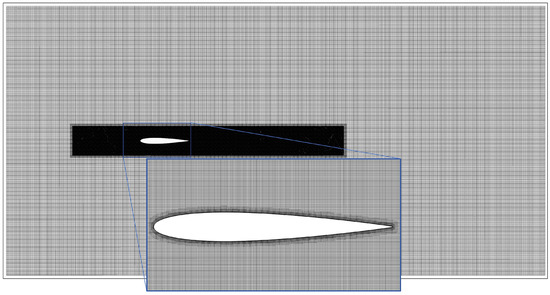
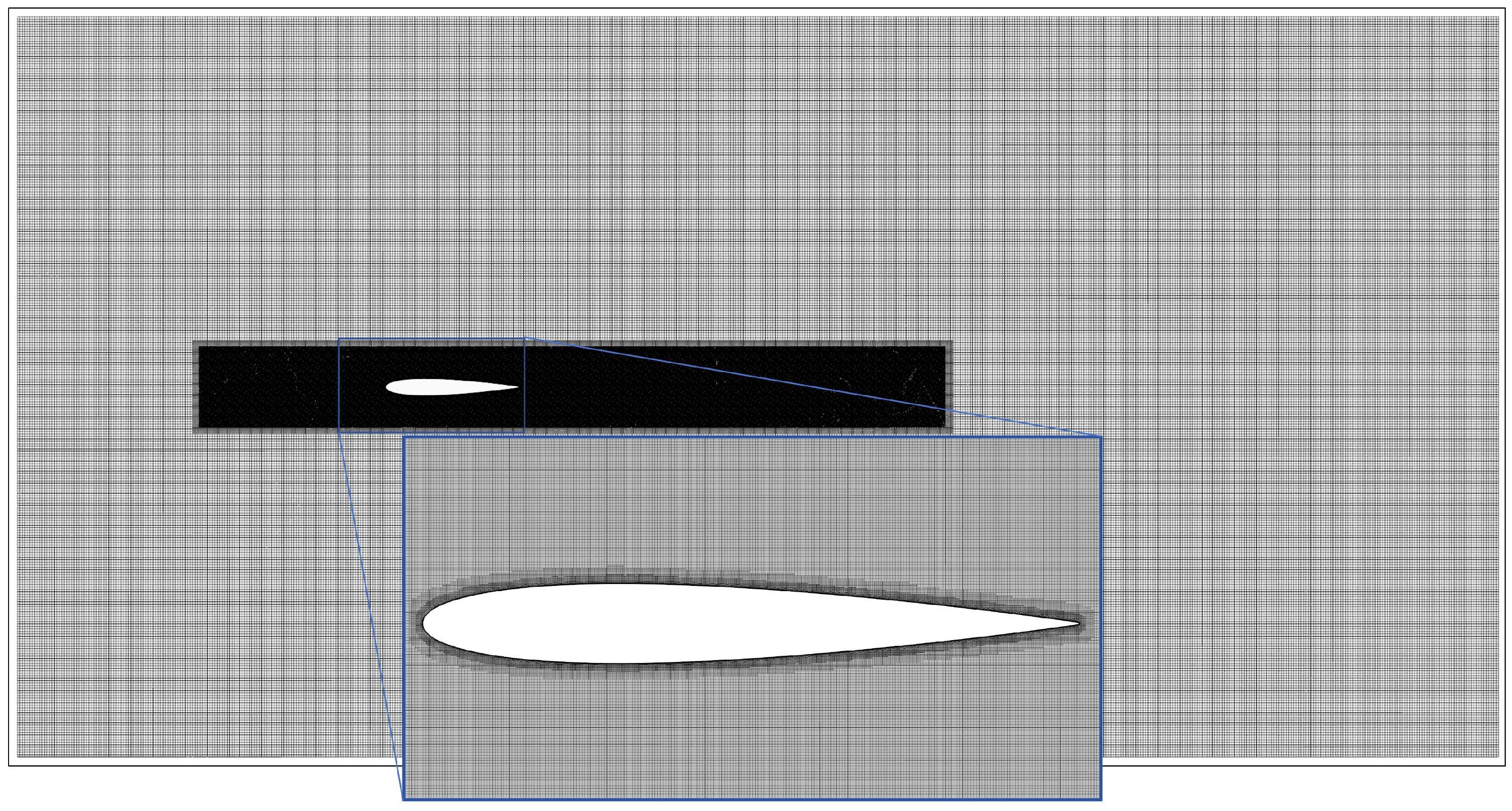
To validate the accuracy of the present numerical method, a verification study is first conducted for a single swimming fish. Figure 1 shows the computational domain. The fish has a body length of L, and the domain size is . With the fish head as the reference point, the inlet boundary is located at upstream, the outlet at downstream, and the lateral walls at from the fish. The inlet is set as a velocity inlet, the outlet as a pressure outlet, and the lateral boundaries as slip walls. A no-slip condition is imposed on the fish surface. The mesh configuration is illustrated in Figure 2. An overset mesh method is employed, consisting of a background mesh for the computational domain and a refined overlapping mesh region around the fish. Local grid refinement is applied near the fish body and in its wake to accurately resolve the boundary layer flow, capture the wake vortex evolution, and improve numerical accuracy in regions with potential multi-body interactions.
Figure 2.
Mesh configuration of the computational domain.
In the present boundary layer setup, a prism layer mesh with 10 layers and a stretching ratio of 1.2 was adopted to resolve the boundary layer. The first-cell height was approximately m, and the total prism layer thickness was about m. The resulting dimensionless wall distance was , which is well below the recommended threshold of 5 for laminar flow simulations, ensuring adequate resolution of the viscous sublayer.
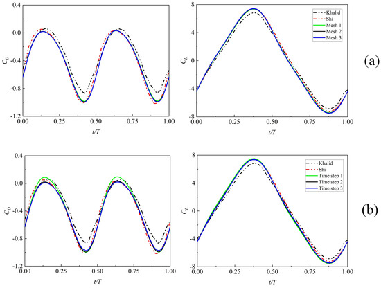
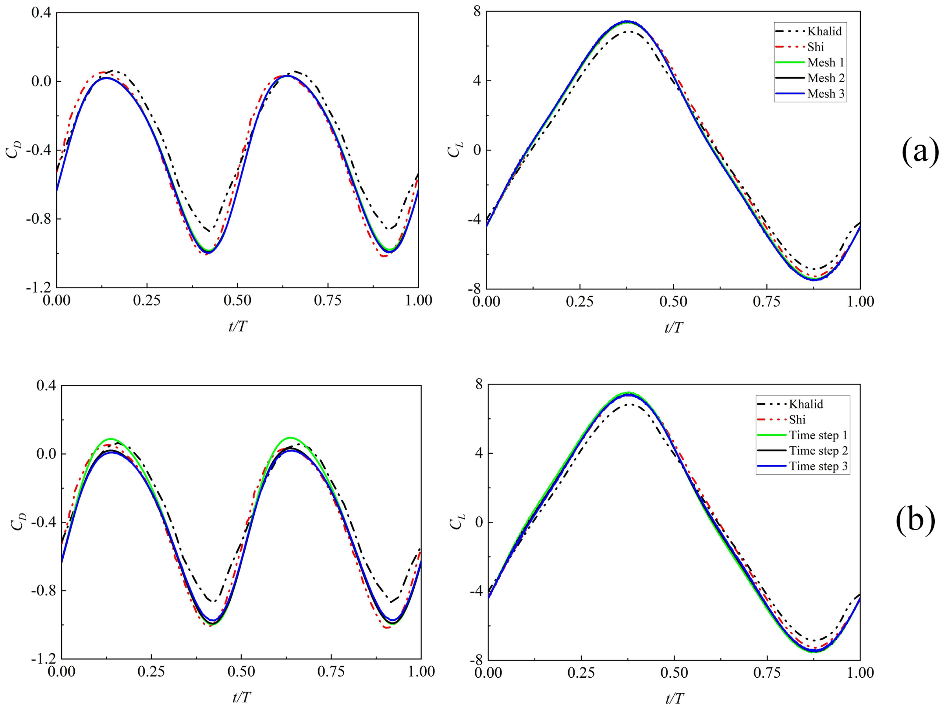
To systematically validate the reliability of the present numerical method, the single-fish case was first computed using Mesh 2 and Time step 2 as the baseline configuration, and the results were compared with those of Khalid et al. [18] and Shi et al. [25]. Figure 3 presents the time histories of the drag and lift coefficients over one cycle at , where the black dashed line denotes the results of Khalid et al. [18], the red dashed line denotes the results of Shi et al. [25], and the solid line corresponds to the present simulations. As shown in Figure 3, the present time histories are in good agreement with both reference datasets in terms of waveform and amplitude.
Figure 3.
Time histories of drag and lift coefficients for (a) different grids and (b) different time steps.
To quantitatively assess the reliability of the method, Table 2 summarizes the relative errors of the key force coefficients obtained from the present simulations with respect to the reference values of Khalid et al. [18] and Shi et al. [25]. Here, and denote the root-mean-squared values of the drag and lift coefficients, respectively; is the time-averaged drag coefficient; and is the maximum lift coefficient. Compared with the reference values of Khalid et al. [18] (, ), the relative errors in and are 11.94% and 7.27%, respectively. Compared with the reference values of Shi et al. [25] (, ), the relative errors in and are 4.78% and 1.17%, respectively. These quantitative comparisons further confirm the reliability of the present numerical method.
Table 2.
Comparison of force coefficients with the reference values of Khalid et al. [18] and Shi et al. [25].
On this basis, the time step was fixed at Time step 2, and three grids with different resolutions—Mesh 1, Mesh 2, and Mesh 3, with approximately 417,000, 512,000, and 631,000 cells, respectively—were employed for the grid independence study. Similarly, the grid was fixed at Mesh 2, and three different time steps—Time step 1 (), Time step 2 (), and Time step 3 ()—were adopted for the time-step independence study. Table 3 and Table 4 summarize the key force coefficients obtained from the grid and time-step independence studies, together with the percentage differences between Mesh 2 and Mesh 3, and between Time step 2 and Time step 3, respectively. The percentage differences between Mesh 2 and Mesh 3 for , , , and are 0.47%, 0.11%, 0.27%, and 0.32%, respectively. All key quantities vary by less than 1%, indicating that the adjacent grid levels differ negligibly. For Time step 2 and Time step 3, the percentage differences for the same quantities are 0.93%, 0.23%, 3.85%, and 0.38%, respectively, all within 4%, confirming that the adjacent time steps also differ only marginally. Considering both computational accuracy and cost, Mesh 2 and Time step 2 are selected as the grid resolution and time-step size for all subsequent simulations.
Table 3.
Mesh independence results.
Table 4.
Time-step independence results.
To assess the sensitivity of the present results to the computational domain size, additional simulations were performed for a representative case (Case 2) using two larger domains: and . Table 5 compares the time-averaged thrust coefficients() obtained with the three domain sizes for each fish, with the changes calculated relative to the original domain. The variations between the original domain and the two larger domains are all within for all three fish. Moreover, the differences between the and results are marginal, indicating that further enlargement of the domain would have only a minor effect on the results. Based on the above results, the computational domain of is adopted in this study.
Table 5.
Domain-size sensitivity of for Case 2.
3. Results and Discussion
3.1. Effects of Streamwise Spacing on Hydrodynamic Performance
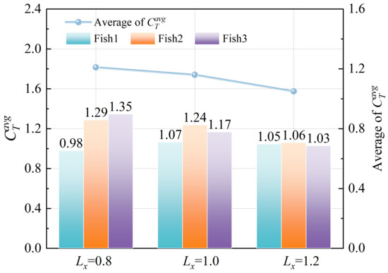
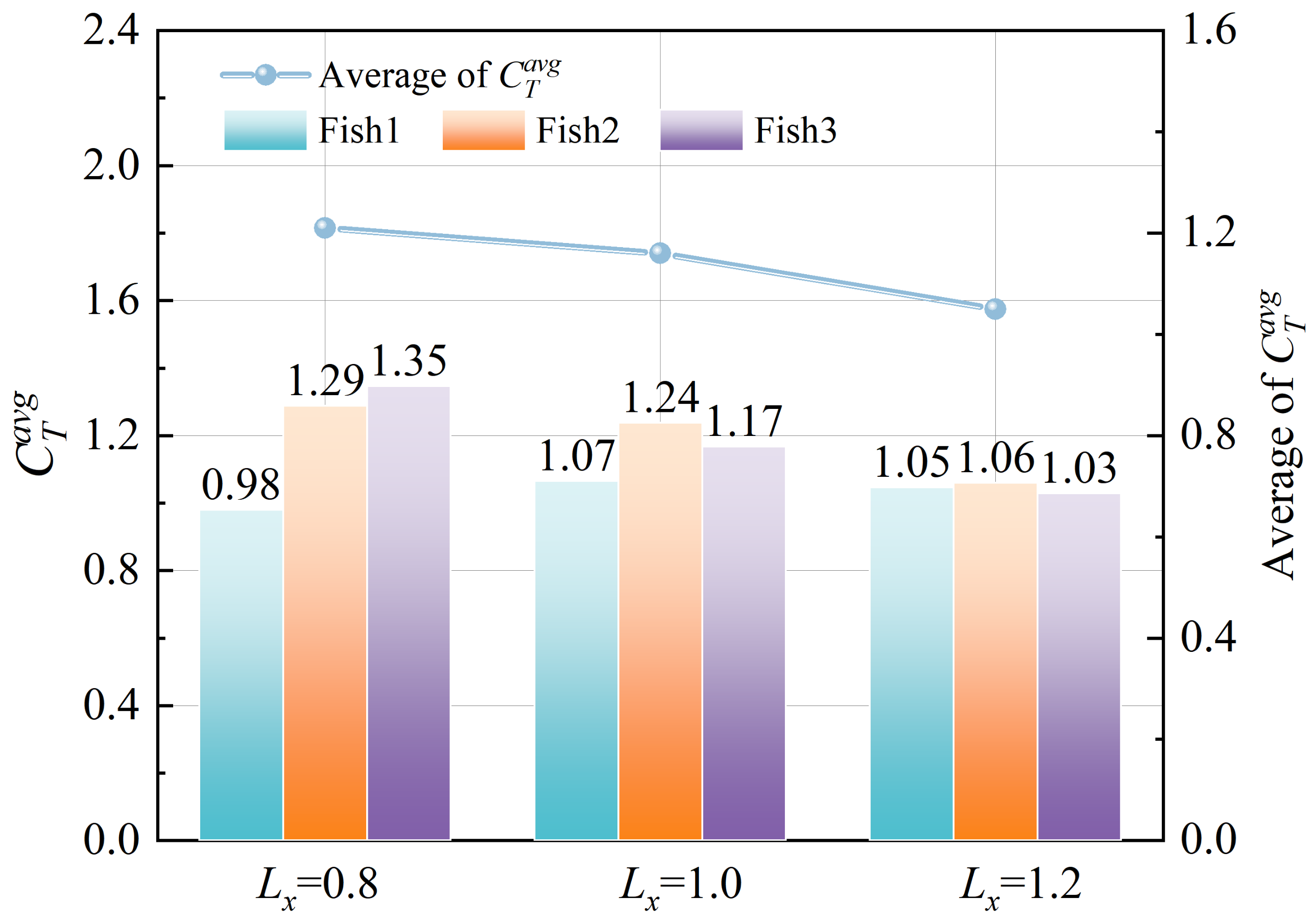
The bar chart in Figure 4 presents the time-averaged thrust coefficient for each fish under different streamwise spacings. This ratio, defined as the thrust coefficient of an individual in the school normalized by that of a solitary swimmer, is introduced in Section 2.
Figure 4.
Individual and overall time-averaged thrust coefficients of the three-fish school for different streamwise spacings.
For Case 1 (, ), the thrust of Fish1 slightly decreases by 2%, while Fish2 and Fish3 exhibit increases of 29% and 35%, respectively. In Case 2 (, ), all three fish show thrust enhancement: Fish1 increases by 7%, Fish2 by 24%, and Fish3 by 17%. In Case 3 (, ), the improvements are modest, with Fish1, Fish2, and Fish3 increasing by 5%, 6%, and 3%, respectively.
These results indicate that at a small streamwise spacing, Fish1 experiences a slight thrust reduction, whereas Fish2 and Fish3 benefit from positive gains. As the spacing increases, the thrust penalty on Fish1 diminishes and eventually turns into a small positive gain, while the benefits for Fish2 and Fish3 gradually decrease. When , the thrust coefficients of all three fish approach that of a solitary swimmer, suggesting that the mutual interference becomes negligible at larger spacings. In summary, as the streamwise spacing increases, the thrust gain of Fish1 increases slightly, while that of Fish2 and Fish3 progressively declines.
The curve in Figure 4 shows the overall time-averaged thrust coefficient of the three-fish school as a function of streamwise spacing. In general, the collective thrust gain decreases with increasing spacing and gradually approaches the value of a solitary swimmer.
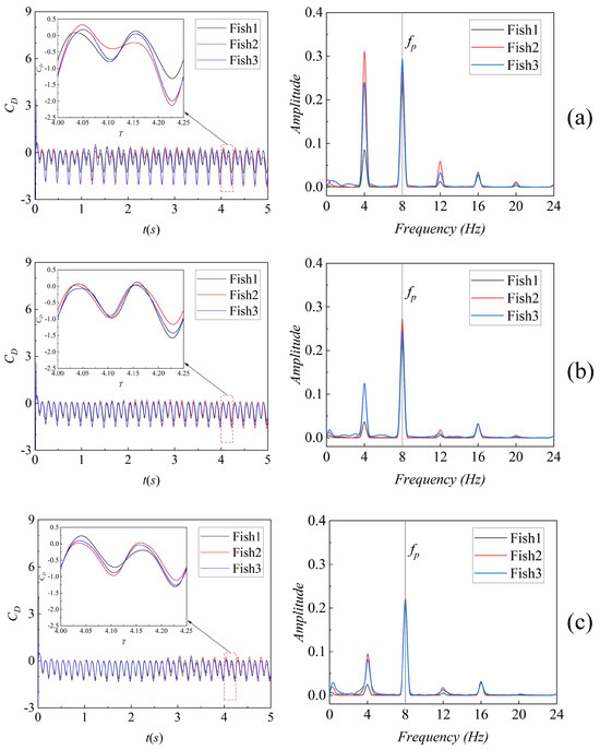
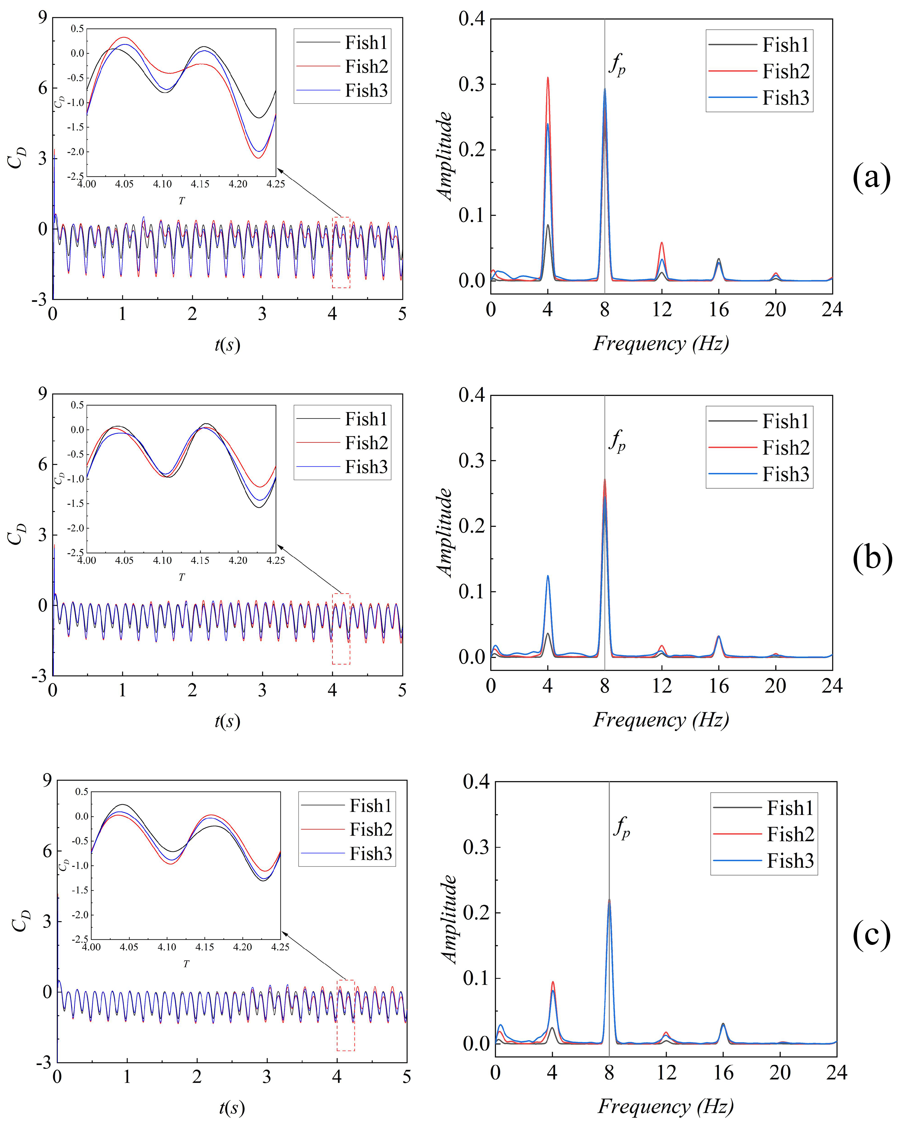
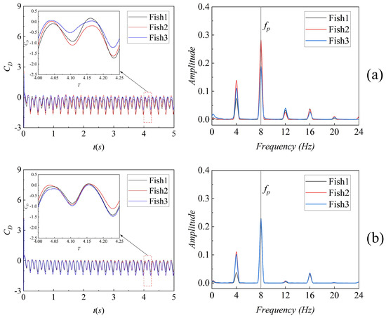
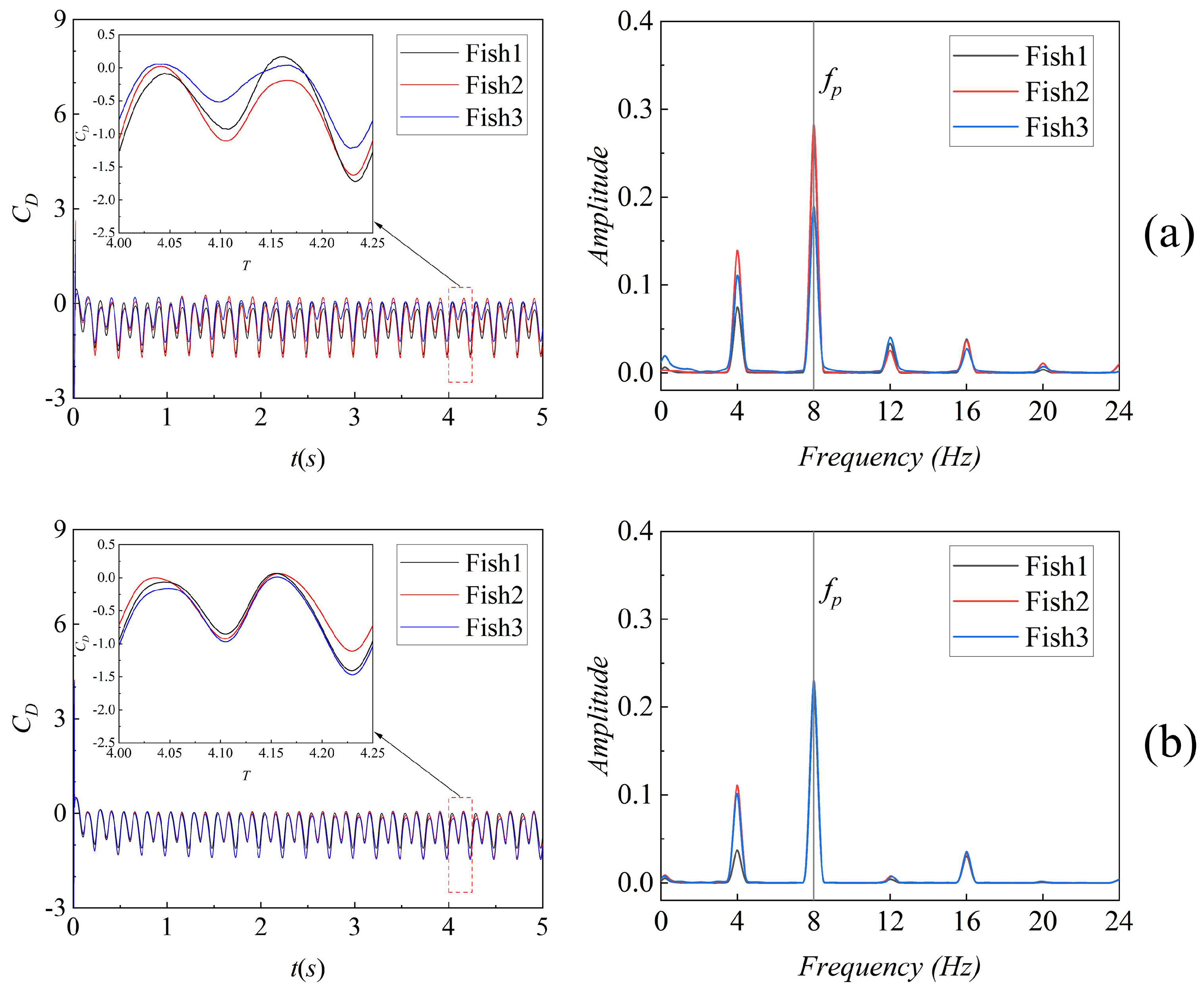
To gain further insight into the interaction mechanisms among biomimetic fish at different streamwise spacings, the time histories of the drag coefficient for each fish (left column of Figure 5) are analyzed, and their corresponding frequency spectra obtained via fast Fourier transform (FFT) are presented in the right column of Figure 5. For the FFT analysis, the first 10 cycles were discarded as transients, and the subsequent 10 stable cycles were used. The sampling frequency was , with , which is well above the Nyquist frequency and sufficient to resolve the dominant frequency and its harmonics. Prior to the transform, a linear trend was removed and a Hanning window was applied to reduce spectral leakage. The spectral amplitudes were normalized to the single-sided spectrum by , with the DC component () treated separately.
Figure 5.
Frequency spectra of the drag coefficient for each fish at different streamwise spacings: (a) Case 1, (b) Case 2, (c) Case 3.
Figure 5a–c correspond to Cases 1, 2, and 3, respectively. For all cases, remains predominantly negative over a cycle, indicating that the net streamwise force acts as thrust. The curves exhibit a double-peak pattern within each period, approximating a sinusoidal oscillation. In the present simulations, the undulation frequency of the fish is . The dominant frequency in the spectra is , which is twice the undulation frequency. This is attributed to the tail beating upward and downward once per cycle, a feature commonly observed in vortex-induced vibration [26] and flapping foils [27].
In Case 1, in addition to the dominant peak at , secondary peaks appear at , along with smaller peaks at and . Fish1 exhibits a single-peak spectral pattern, suggesting weak interaction with the downstream fish. In contrast, Fish2 and Fish3 display double-peak patterns, indicating stronger hydrodynamic interactions. In Case 2, the double-peak features of Fish2 and Fish3 become less pronounced, reflecting a reduction in mutual interference—consistent with the observed decrease in thrust benefit as spacing increases. In Case 3, the spectra of all three fish converge toward a similar shape, implying that the interactions among them become negligible at larger spacings.
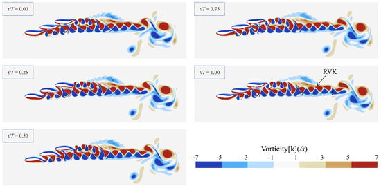
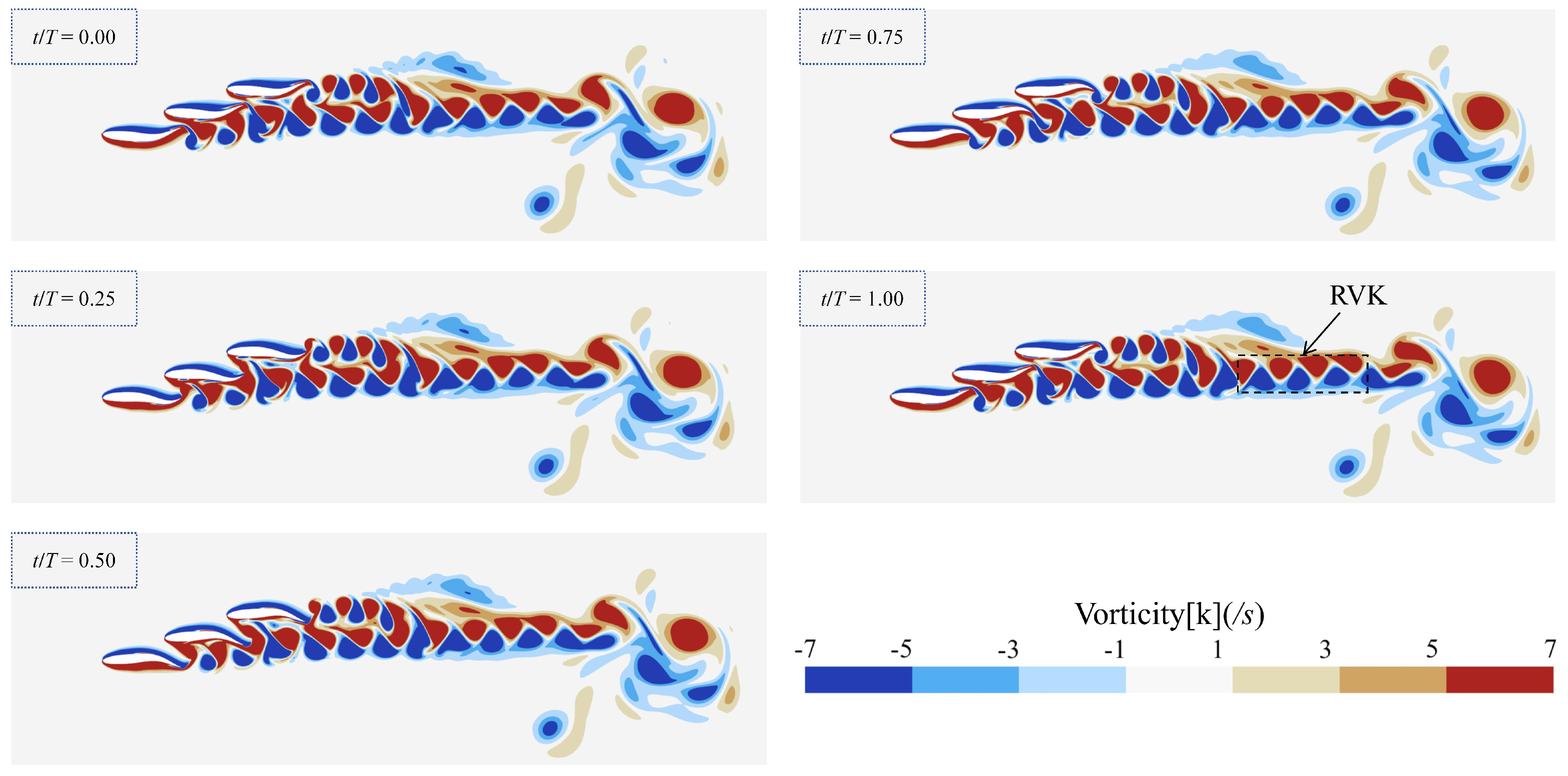
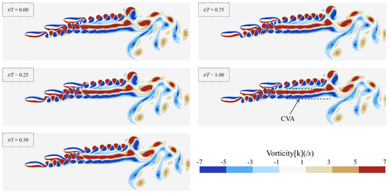
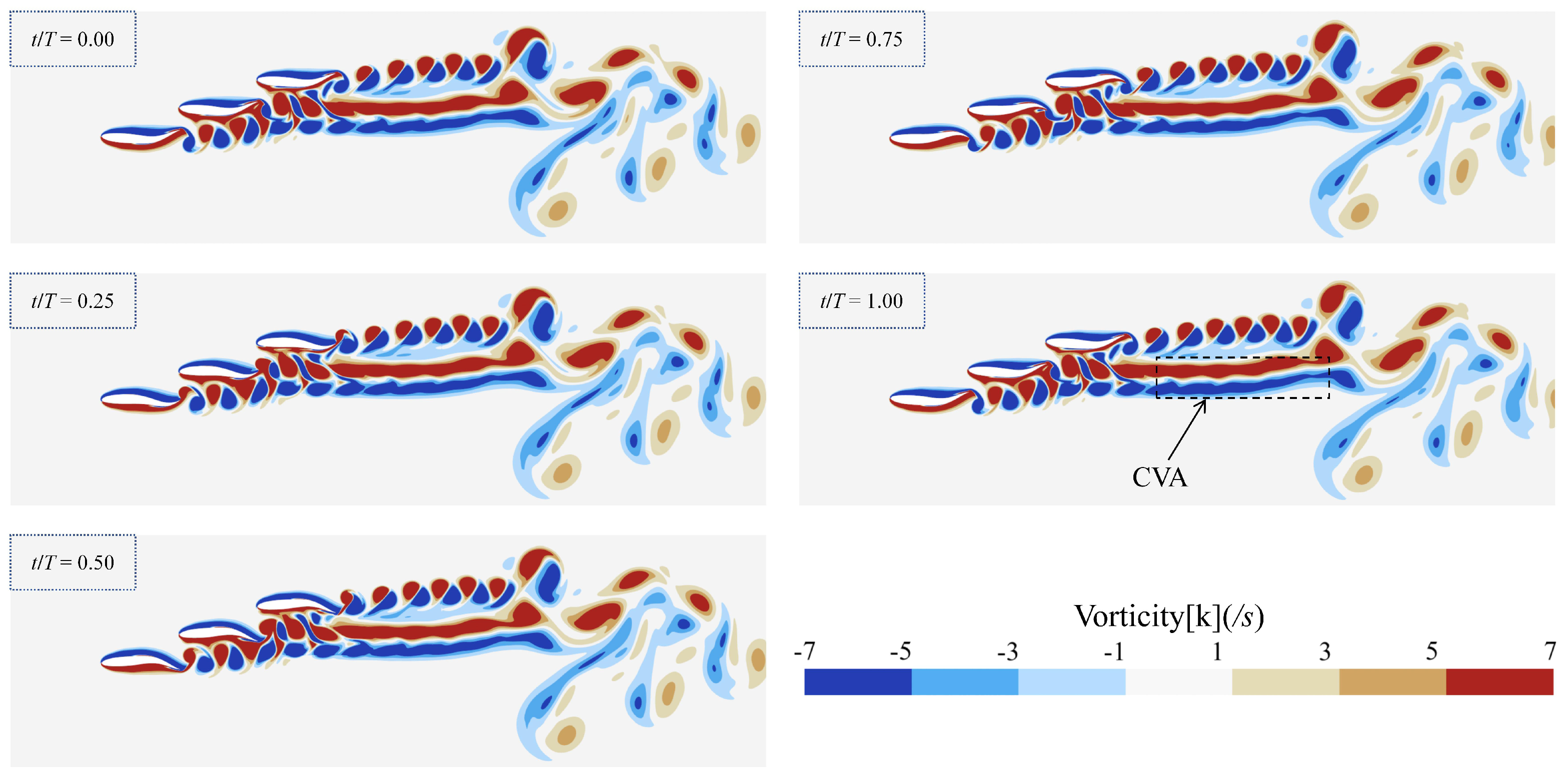
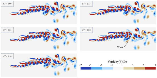
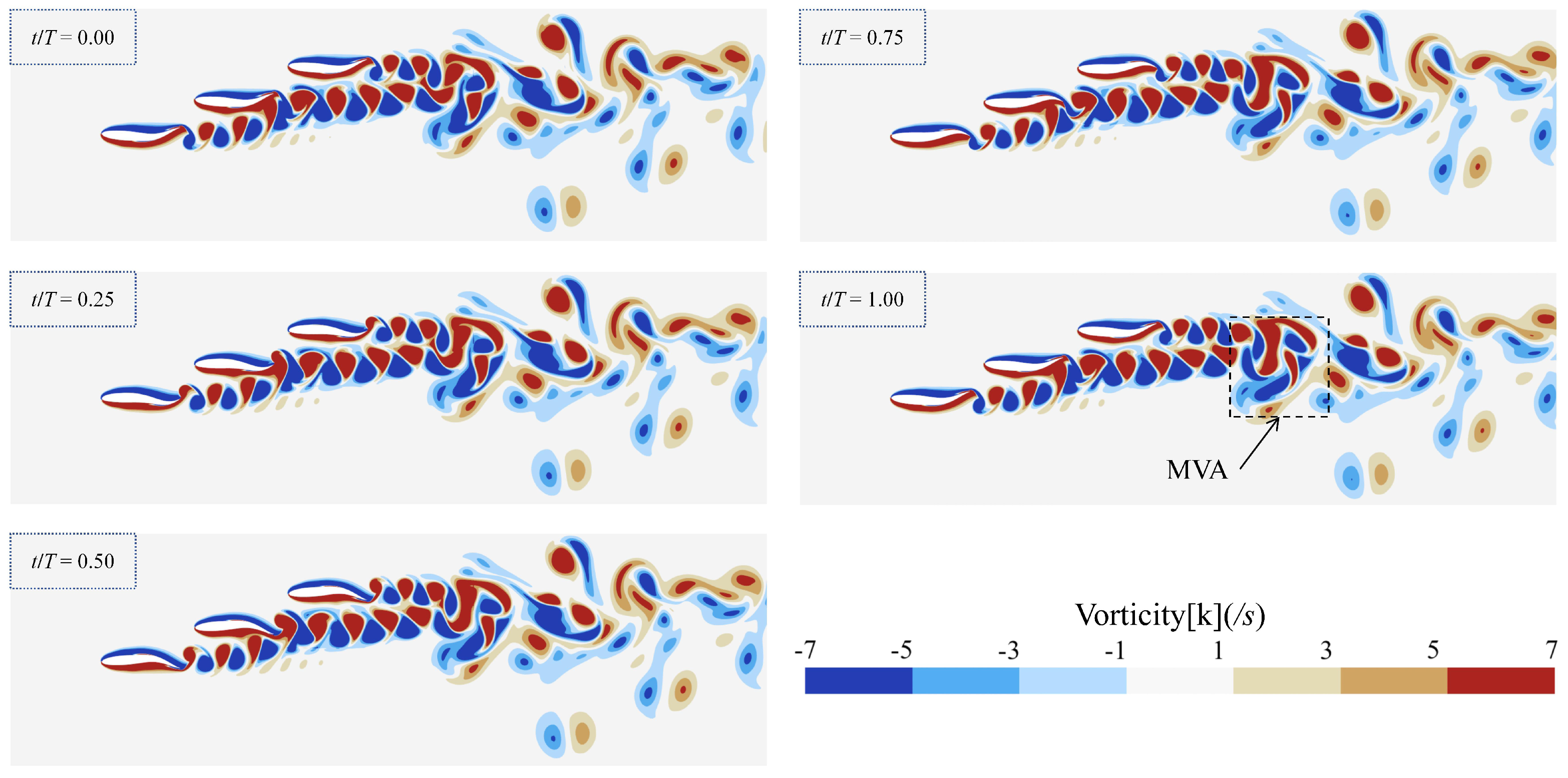
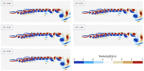
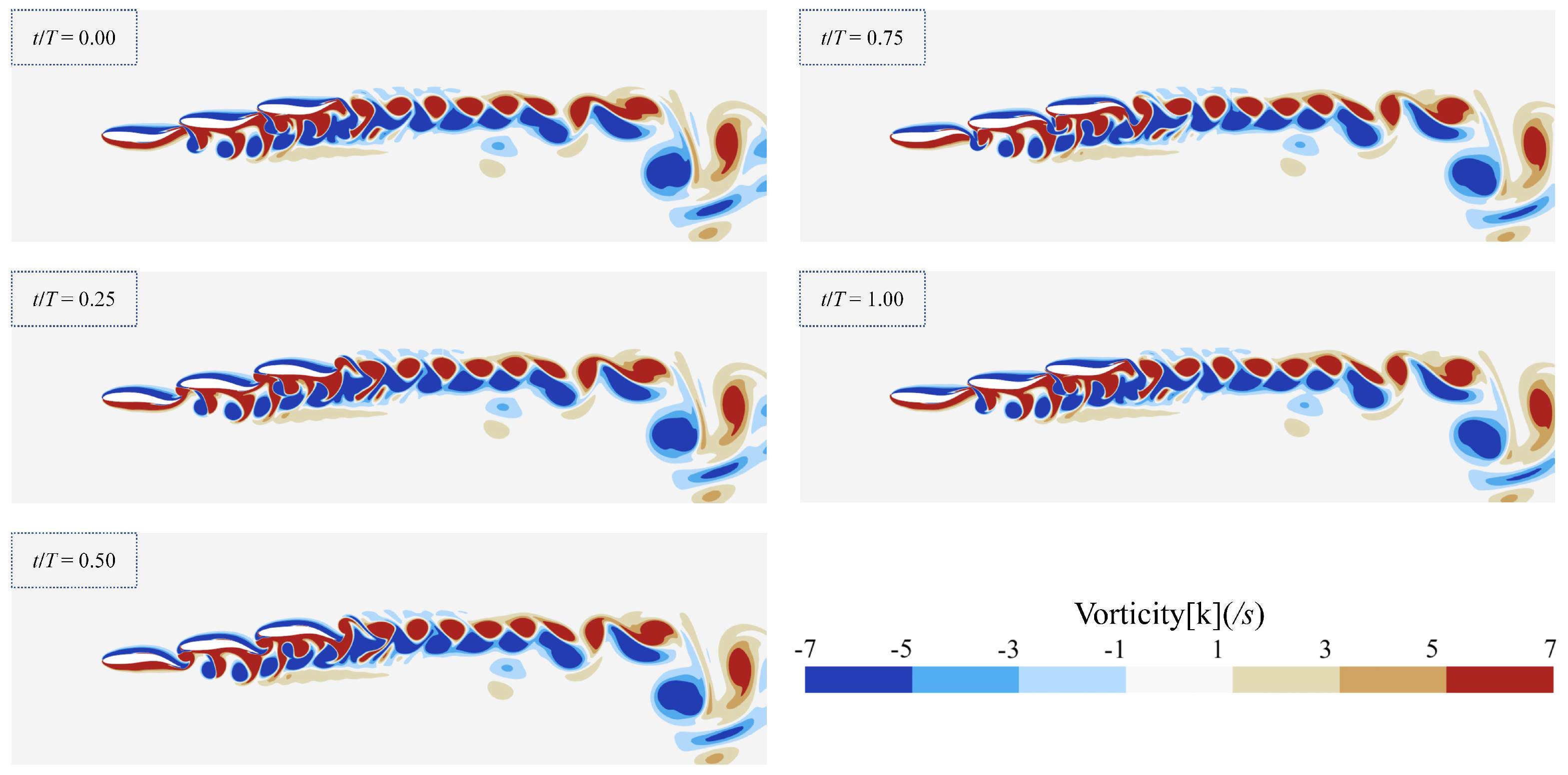
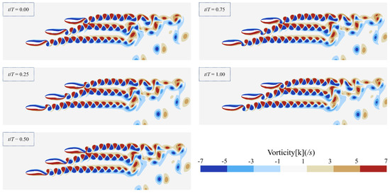
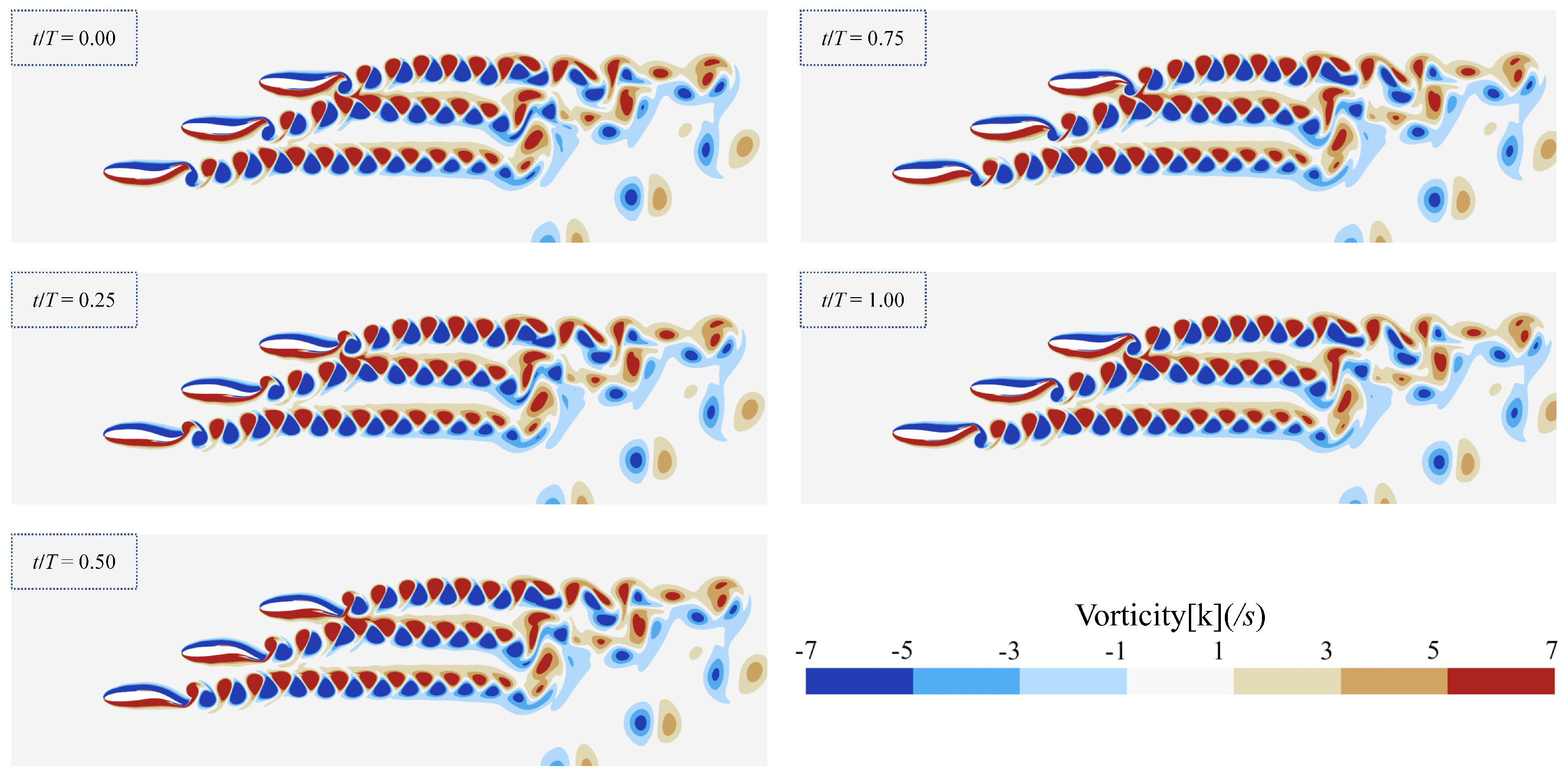
To further illustrate the flow field characteristics around the fish bodies and in the wake regions, the vorticity, pressure, and velocity contours under different cases are presented in the following figures. Figure 6, Figure 7 and Figure 8 show the vorticity contours for each fish over one cycle under different spacing conditions (one representative cycle from the periodically stable state is selected to examine the evolution of the wake vortices). The following labels are used in the figures: the reverse von Kármán vortex street (RVK), the mixing vorticity area (MVA), and the coalescence vorticity area (CVA). By comparing the differences in flow field structures under various spacings and orientation angles, a visual basis at the flow-field level is provided for understanding the multi-body hydrodynamic interactions in fish schooling.
Figure 6.
Time evolution of vorticity contours for Case 1 over one cycle.
Figure 7.
Time evolution of vorticity contours for Case 2 over one cycle.
Figure 8.
Time evolution of vorticity contours for Case 3 over one cycle.
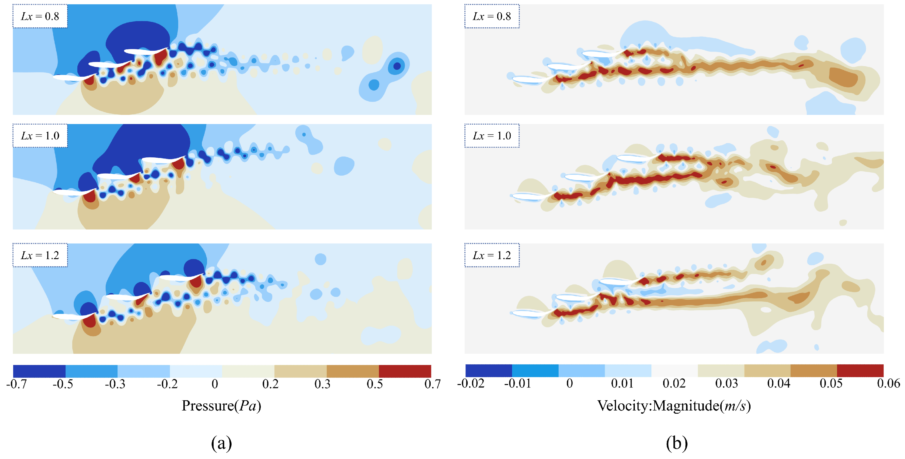
The vorticity contours for Case 1 are shown in Figure 6. The positive vortices shed from the tail of Fish1 propagate downstream along the lower surface of Fish2 and merge with the positive vortices shed from Fish2 near its tail. Meanwhile, the merged vortex structure continues to propagate downstream, and part of the positive combined vortex interacts with the wake of Fish3 near its tail. Eventually, all vorticity coalesces farther downstream into a row of RVK. In contrast, no noticeable merging is observed in the wake structure behind the tail of Fish1. In the velocity field (Figure 9b), jet regions consistent with the propagation path of the vorticity are observed downstream of the tails of Fish2 and Fish3.
Figure 9.
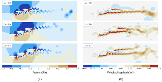
Pressure and velocity fields for different streamwise spacings at : (a) pressure field, (b) velocity field.
The vorticity contours for Case 2 are shown in Figure 7. The positive vortices shed from Fish1 merge with those from Fish2 near the tail of Fish2. Meanwhile, the negative vortices shed from Fish1 accumulate in the same region downstream of Fish2. For Fish3, an accumulation of negative vortices is observed on its left side, and a relatively large spatial gap exists between the upstream merged vortices and the wake of Fish3. Downstream of Fish3, the vortex arrangement is more dispersed compared to that in Case 1. The combined vortices of Fish1 and Fish2 merge into a CVA downstream. Ultimately, two distinct wake structures propagate downstream: an RVK formed behind Fish3, and the CVA originating from Fish1 and Fish2.
The vorticity contours for Case 3 are shown in Figure 8. Compared with Cases 1 and 2, as the streamwise spacing increases, the wakes of the three fish become more separated and the degree of interaction decreases. Near the tail of Fish2, vortex merging is still observed, whereas no significant merging is visible at the tail of Fish3. The combined vortices of Fish1 and Fish2 merge with those of Fish3 farther downstream, forming an irregular MVA.
The pressure and velocity fields underlying these thrust characteristics are shown in Figure 9. Figure 9a shows the pressure contours at for different spacings. For Case 1, a strong low-pressure region forms between the tail of Fish1 and the head of Fish2, completely enveloping the head of Fish2. Similar low-pressure regions are also observed near the head and upper side of Fish3. In the velocity field shown in Figure 9b, the wake of Fish1 spatially merges with the wake of Fish2 near the tail of Fish2. The combined jet then merges with the downward-deflected jet from Fish3, and they propagate downstream together.
For Case 2, the low-pressure regions at the tails of Fish1 and Fish2 no longer connect with those at the heads of Fish2 and Fish3. The wake of Fish1 is deflected upward, and the two jets merge near the tail of Fish2, corresponding to the CVA observed in Figure 7. The wake of Fish3, however, does not merge with this jet, resulting in two separate jets propagating downstream of Fish3.
For Case 3, as the spacing further increases, the pressure regions near the heads and tails of the three fish become separated from one another. The wake of Fish1 is deflected upward under the influence of Fish2, and the jet eventually dissipates within the MVA.
3.2. Analysis of Biomimetic Fish Swimming Under Different Arrangement Angles
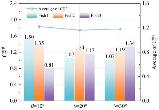
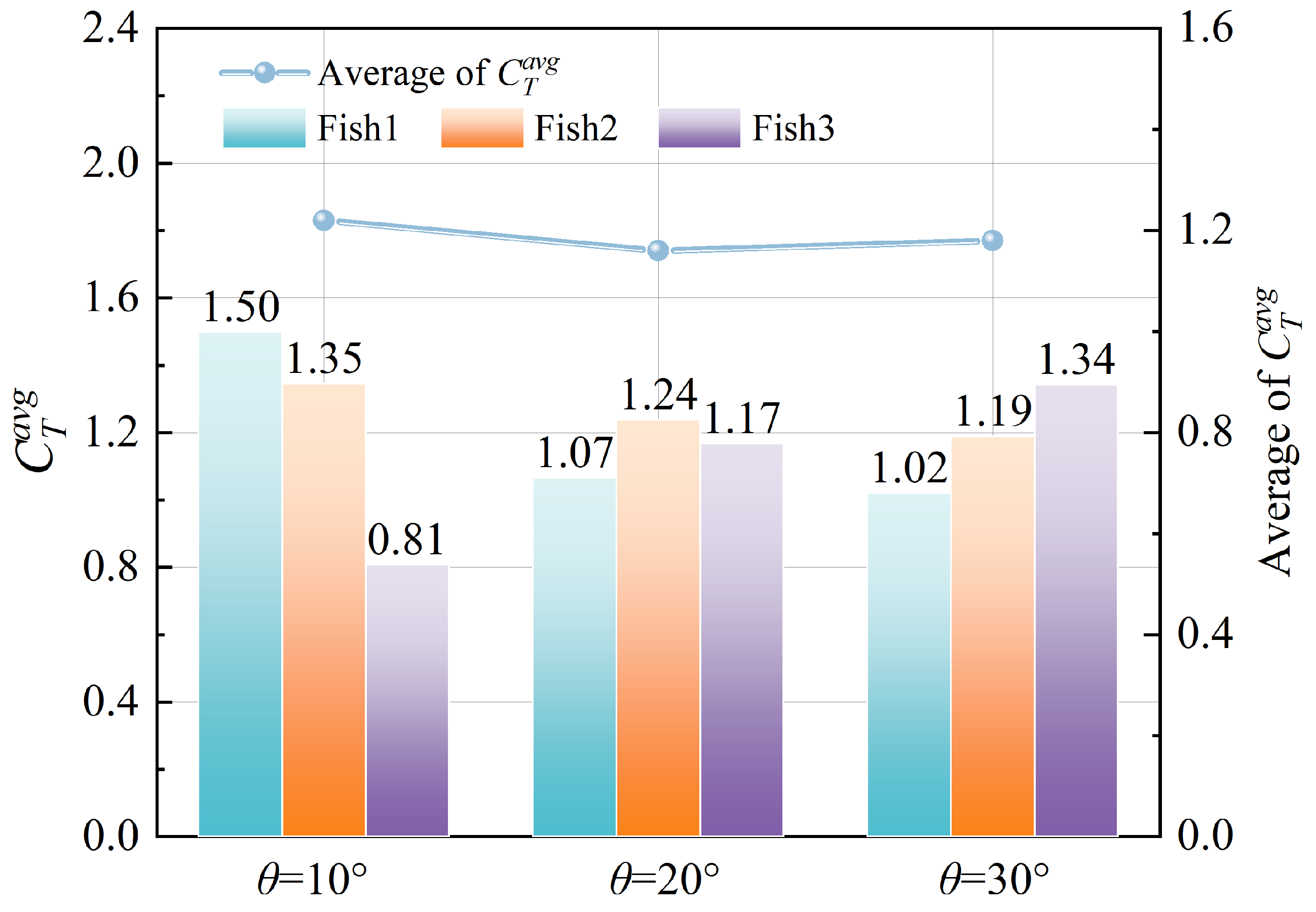
The bar chart in Figure 10 presents the normalized time-averaged thrust coefficient for each fish at different orientation angles. In Case 4 (, ), the thrust of Fish1 and Fish2 increases, while that of Fish3 decreases. Specifically, the thrust of Fish1 increases by 50% and that of Fish2 by 35%, and that of Fish3 decreases by 19%. In Case 5 (, ), all three fish exhibit thrust enhancement: Fish1 shows a modest increase of 2%, the thrust of Fish2 increases by 19%, and that of Fish3 increases by 34%.
Figure 10.
Individual and overall time-averaged thrust coefficients of the three-fish school for different orientation angles.
These results indicate that at a small orientation angle, Fish1 and Fish2 experience positive thrust gains, with Fish1 benefiting the most, whereas Fish3 suffers a thrust penalty. As the orientation angle increases, the thrust gains for Fish1 and Fish2 gradually diminish, while the thrust of Fish3 transitions from negative to positive. At , the gains for Fish1 and Fish2 continue to decline, whereas Fish3 shows further improvement.
In summary, as the orientation angle increases, the thrust gain of Fish1 and Fish2 progressively decreases, while that of Fish3 increases. The curve in Figure 10 shows the overall time-averaged thrust coefficients for the three-fish school as a function of orientation angle. Overall, the collective thrust gain initially decreases and then plateaus as the angle increases. This plateau occurs because the increase in thrust for Fish3 slightly outweighs the combined decrease for Fish1 and Fish2, resulting in a nearly constant overall value.
To further elucidate the hydrodynamic interactions among biomimetic fish at different orientation angles, the time histories of the drag coefficient for each fish (left column of Figure 11) are examined, and their corresponding frequency spectra obtained via fast Fourier transform (FFT) are presented in the right column of Figure 11.
Figure 11.
Frequency spectra of the drag coefficient for each fish at different orientation angles: (a) Case 4, (b) Case 5.
Figure 11a,b correspond to Cases 4 and 5, respectively. For all cases, remains predominantly negative over a cycle, indicating that the net streamwise force acts as thrust. The dominant frequency in the spectra is , which is twice the undulation frequency.
In Case 4, in addition to the dominant peak at , notable harmonic peaks appear at and , indicating stronger nonlinear interactions compared to the other cases. In Case 2, the spectral peaks at , , and for Fish1 and Fish2 diminish, reflecting reduced mutual interference. Meanwhile, the peaks at and for Fish3 become more pronounced, suggesting enhanced nonlinear effects. In Case 5, the harmonic peaks at for Fish1 are small, indicating weak nonlinear interactions, whereas Fish2 and Fish3 retain noticeable peaks at , implying that nonlinear effects persist for these individuals.
These results indicate that as the orientation angle increases, the influence on Fish1 diminishes, while nonlinear interactions remain significant for Fish2 and Fish3. This trend is consistent with the variation in time-averaged thrust discussed previously: as increases, the thrust of Fish1 approaches that of a solitary swimmer, whereas Fish2 and Fish3 continue to experience nonlinear effects.
Figure 12 and Figure 13 show the vorticity contours of the flow field for each fish over one cycle under different orientation angles. The vorticity contours for Case 4 are shown in Figure 12. The positive vortices shed from Fish1 propagate along the left side of Fish2. The lateral spread of the vortex structures in the downstream wake region of Fish1 and Fish2 is relatively small. In contrast, the vorticity distribution downstream of Fish3 is more dispersed. Near the region where Fish2 generates positive vortices, the negative vortices shed from Fish1 accumulate in the same area. The wakes of Fish1 and Fish2 merge on the left side of Fish3 and continue to propagate downstream.
Figure 12.
Time evolution of vorticity contours for Case 4 over one cycle.
Figure 13.
Time evolution of vorticity contours for Case 5 over one cycle.
The vorticity contours for Case 2 are shown in Figure 7. Compared with Case 4, the lateral spacing between the fish bodies is larger. The vortices of Fish1 and Fish2 partially overlap in space and extend into the wake region of Fish3.
The vorticity contours for Case 5 are shown in Figure 13. As the orientation angle increases, the lateral spacing between the fish becomes larger. The positive vortices shed from Fish1 propagate downstream, with a small portion merging with the vortices of Fish2. The wakes of Fish2 and Fish3 partially merge in space.
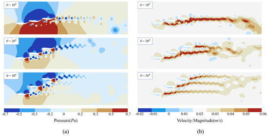
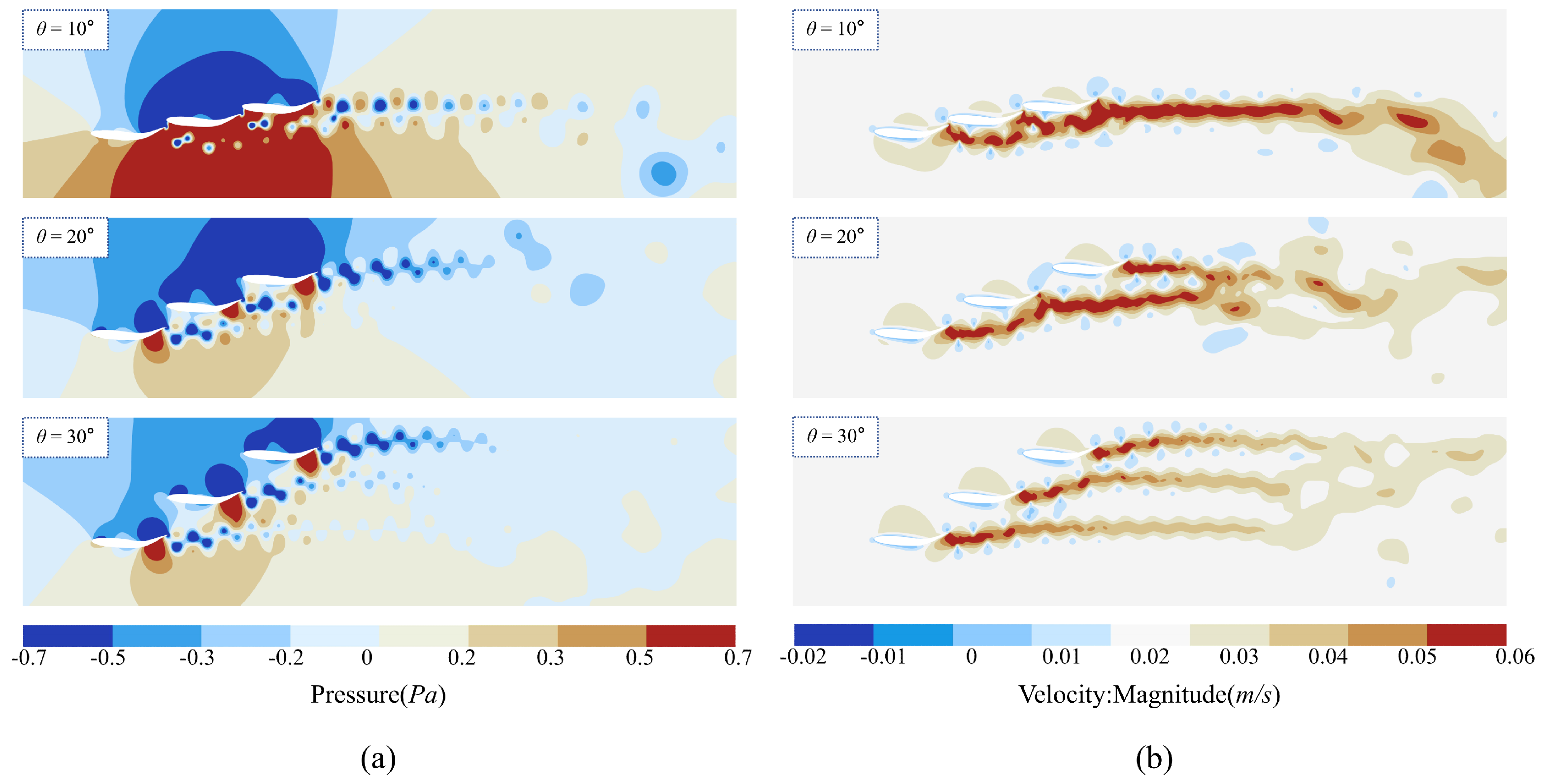
Figure 14 shows the (a) pressure and (b) velocity contours at for different orientation angles. For Case 4, which has a relatively small orientation angle, Figure 14a reveals a distinct low-pressure region on the upper surface near the tail of Fish1, the side of Fish2, and the head of Fish3. Concurrently, a high-pressure region appears on the lower surface near the tail of Fish1, the side of Fish2, and the side of Fish3. In the velocity field (Figure 14b), the jets from the tails of each fish propagate downstream, and merging of the jets is observed near the tails of Fish2 and Fish3. Subsequently, a single jet continues to propagate downstream of Fish3.
Figure 14.
Pressure and velocity fields for different orientation angles at : (a) pressure field, (b) velocity field.
For Case 2, the spatial extents of both the high-pressure and low-pressure regions on each fish surface are reduced compared with Case 4. In the velocity field, the jet generated by Fish1 merges with that of Fish2 in the downstream region of Fish2. The merged jet then propagates side by side with the trailing jet of Fish3.
For Case 5, the pressure regions on the surfaces of each fish become independent, with no significant interconnection observed. In the velocity field, the three jets from the three fish remain separate, and no obvious merging is observed.
4. Conclusions
In this study, the hydrodynamic performance of three biomimetic fish in an oblique tandem arrangement is examined for selected streamwise spacings and orientation angles, with a focus on the time-averaged thrust coefficient, wake structures, and flow field characteristics. The main conclusions are as follows:
(1) For the three-fish oblique tandem arrangement, the overall time-averaged thrust coefficient of the school is higher than that of a solitary swimmer, with an increase ranging from 16% to 22%. As the streamwise spacing increases, the collective thrust gain decreases and gradually approaches that of a solitary swimmer. As the orientation angle increases, the collective thrust gain initially decreases and then plateaus.
(2) For different streamwise spacings within the present range, as the spacing increases, the thrust of Fish1 remains relatively stable and approaches that of a solitary swimmer. In contrast, the thrust coefficients of Fish2 and Fish3 gradually decrease due to reduced mutual interference, eventually approaching that of a solitary swimmer at .
(3) For different orientation angles, as the angle increases, the lateral spacing between adjacent fish increases accordingly. The time-averaged thrust coefficients of Fish1 and Fish2 gradually decrease and approach that of a solitary swimmer, while the thrust coefficient of Fish3 progressively increases, transitioning from a thrust penalty to a thrust gain.
(4) At a small orientation angle (, ), the lateral spacing between adjacent fish is relatively small. In the narrow gap between Fish1 and Fish2, the vorticity distribution exhibits a reduced lateral spread, and the time-averaged thrust coefficients of both Fish1 and Fish2 are higher than that of a solitary swimmer.
Based on the five representative cases examined in this study, the present work provides a preliminary investigation of the effects of streamwise spacing and orientation angle on the thrust performance, vortex structure, and flow field characteristics when three fish are in an oblique tandem arrangement. Within the present parameter space, the thrust gain is found to decrease as the spacing increases, and first decreases then stabilizes as the arrangement angle increases; similarly, regarding the transformation mechanism, the thrust of the tail fish turns from negative to positive. These results suggest that a proper combination of spacing and orientation angle can modulate the thrust performance of the fish school.
It should be noted that the present study adopts a two-dimensional model and does not account for three-dimensional effects such as spanwise flows and tip vortices. In reality, three-dimensional flow features influence wake structures and thrust distribution, and a two-dimensional model may not fully capture these effects. Second, only five representative parameter combinations are examined. In real fish schools, orientation angles and spacings vary continuously, and the current discrete cases, while revealing general trends, do not cover the entire parameter space. Third, the classification of wake structures (RVK, MVA, and CVA) is based primarily on qualitative observation of vorticity contours. In real flows, quantitative metrics such as vortex circulation and jet angle are more indicative of interaction intensity, and the current qualitative classification does not yet provide sufficient quantitative support. Future work may proceed along the following directions: three-dimensional simulations and quantitative validation under self-propelled models, denser parametric sweeps, and the introduction of quantitative diagnostics such as vortex circulation. The results presented here provide a preliminary basis for understanding the fluid interactions in oblique tandem arrangements within the present parameter space.
Author Contributions
Conceptualization, J.H.; methodology, J.H., Y.C. and J.Y.; software, J.L. and B.H.; validation, J.L. and B.H.; formal analysis, J.L. and B.H.; investigation, J.H., Y.C. and Z.D.; resources, J.H.; data curation, B.H.; writing—original draft preparation, J.L.; writing—review and editing, Y.C., Z.D. and J.Y.; visualization, B.H.; supervision, J.H.; funding acquisition, J.H. All authors have read and agreed to the published version of the manuscript.
Funding
This research received funding from the Ocean Young Talent Innovation Programme of Zhanjiang City (Grant No. 2022E05002), the Young Innovative Talents Grants Programme of Guangdong Province (Grant No. 2022KQNCX024), the China Institute of Navigation Young Elite Scientist Sponsorship Program by CIN (Grant No. YESSCIN2023008), the College Student Innovation Team of Guangdong Ocean University (Grant No. CXTD2021013), the Student Innovation Team of Guangdong Ocean University’s College of Port and Maritime Industry and Technology (Grant No. GHCY2024015), and the Innovation and Entrepreneurship Training Program for College Students (Grant No. CXXL2024217).
Institutional Review Board Statement
Not applicable.
Informed Consent Statement
Not applicable.
Data Availability Statement
The dataset is available on request from the authors.
Conflicts of Interest
The authors declare no conflicts of interest.
References
- Weihs, D. Hydromechanics of Fish Schooling. Nature 1973, 241, 290–291. [Google Scholar] [CrossRef] [Scilit]
- Magurran, A.E.; Higham, A. Information Transfer across Fish Shoals under Predator Threat. Ethology 1988, 78, 153–158. [Google Scholar] [CrossRef] [Scilit]
- Wolf, N.G. Schooling tendency and foraging benefit in the ocean surgeonfish. Behav. Ecol. Sociobiol. 1987, 21, 59–63. [Google Scholar] [CrossRef] [Scilit]
- Ligman, M.; Lund, J.; Fürth, M. A comprehensive review of hydrodynamic studies on fish schooling. Bioinspir. Biomim. 2024, 19, 011002. [Google Scholar]
- Gray, J. Studies in Animal Locomotion, VI. The Propulsive Powers of the Dolphin. J. Exp. Biol. 1936, 13, 192–199. [Google Scholar] [CrossRef] [Scilit]
- Lighthill, M.J. Note on the swimming of slender fish. J. Fluid Mech. 1960, 9, 305–317. [Google Scholar] [CrossRef] [Scilit]
- Wu, T.Y.T. Swimming of a waving plate. J. Fluid Mech. 1961, 10, 321–344. [Google Scholar] [CrossRef] [Scilit]
- Liao, J.C.; Beal, D.N.; Lauder, G.V.; Triantafyllou, M.S. Fish Exploiting Vortices Decrease Muscle Activity. Science 2003, 302, 1566–1569. [Google Scholar] [CrossRef] [Scilit] [PubMed]
- Xiao, Q.; Sun, K.; Liu, H.; Hu, J. Computational study on near wake interaction between undulation body and a D-section cylinder. Ocean Eng. 2011, 38, 673–683. [Google Scholar] [CrossRef] [Scilit]
- Ji, F.; Huang, D. Effects of Reynolds number on energy extraction performance of a two dimensional undulatory flexible body. Ocean Eng. 2017, 142, 185–193. [Google Scholar] [CrossRef] [Scilit]
- Chung, M.-H. Hydrodynamic Performance of Two-Dimensional Undulating Foils in Triangular Formation. J. Mech. 2011, 27, 177–190. [Google Scholar] [CrossRef] [Scilit]
- Kelly, S.D.; Xiong, H. Controlled Hydrodynamic Interactions in Schooling Aquatic Locomotion. In Proceedings of the 44th IEEE Conference on Decision and Control; IEEE: Seville, Spain, 2005; pp. 3904–3910. [Google Scholar]
- Shoele, K.; Zhu, Q. Performance of synchronized fins in biomimetic propulsion. Bioinspir. Biomim. 2015, 10, 026008. [Google Scholar] [CrossRef] [Scilit] [PubMed]
- Tian, F.-B.; Wang, W.; Wu, J.; Sui, Y. Swimming performance and vorticity structures of a mother–calf pair of fish. Comput. Fluids 2016, 124, 1–11. [Google Scholar] [CrossRef] [Scilit]
- Dewey, P.A.; Quinn, D.B.; Boschitsch, B.M.; Smits, A.J. Propulsive performance of unsteady tandem hydrofoils in a side-by-side configuration. Phys. Fluids 2014, 26, 041903. [Google Scholar] [CrossRef] [Scilit]
- Boschitsch, B.M.; Dewey, P.A.; Smits, A.J. Propulsive performance of unsteady tandem hydrofoils in an in-line configuration. Phys. Fluids 2014, 26, 051901. [Google Scholar] [CrossRef] [Scilit]
- Dong, G.-J.; Lu, X.-Y. Characteristics of flow over traveling wavy foils in a side-by-side arrangement. Phys. Fluids 2007, 19, 057107. [Google Scholar] [CrossRef] [Scilit]
- Khalid, M.S.U.; Akhtar, I.; Dong, H. Hydrodynamics of a tandem fish school with asynchronous undulation of individuals. J. Fluids Struct. 2016, 66, 19–35. [Google Scholar] [CrossRef] [Scilit]
- Deng, J.; Shao, X. Hydrodynamics in a diamond-shaped fish school. J. Hydrodyn. 2006, 18, 428–432. [Google Scholar] [CrossRef] [Scilit]
- Park, S.G.; Sung, H.J. Hydrodynamics of flexible fins propelled in tandem, diagonal, triangular and diamond configurations. J. Fluid Mech. 2018, 840, 154–189. [Google Scholar] [CrossRef] [Scilit]
- Li, S.; Li, C.; Xu, L.; Yang, W.; Chen, X. Numerical Simulation and Analysis of Fish-Like Robots Swarm. Appl. Sci. 2019, 9, 1652. [Google Scholar] [CrossRef] [Scilit]
- Triantafyllou, M.S.; Triantafyllou, G.S.; Yue, D.K.P. Hydrodynamics of Fishlike Swimming. Annu. Rev. Fluid Mech. 2000, 32, 33–53. [Google Scholar] [CrossRef] [Scilit]
- Daghooghi, M.; Borazjani, I. The hydrodynamic advantages of synchronized swimming in a rectangular pattern. Bioinspir. Biomim. 2015, 10, 056018. [Google Scholar] [CrossRef] [Scilit] [PubMed]
- Wardle, C.S.; Videler, J. Fish Swimming; Springer Science & Business Media: New York, NY, USA, 1980. [Google Scholar]
- Shi, F.; Tian, Y.; Xin, J.; Ou, C.; Li, Z.; Rao, M. Numerical Study on the Hydrodynamics of Fish Swimming with Different Morphologies in Oblique Flow. J. Mar. Sci. Eng. 2024, 12, 2302. [Google Scholar] [CrossRef] [Scilit]
- Yin, P.; Xin, J.; Shi, F.; Li, Y.; Liu, X.; Shu, L. Numerical study on hydrodynamic interaction characteristics of vortex-induced vibration of two side-by-side cylinders near the wall. Ocean Eng. 2024, 308, 118305. [Google Scholar] [CrossRef] [Scilit]
- Bai, Y.; Zheng, M. Energy harvesting characteristics of a flapping wing with the oscillating aspirators in uniform flows and shear flows. Energy Rep. 2022, 8, 9554–9568. [Google Scholar] [CrossRef] [Scilit]

Disclaimer/Publisher’s Note: The statements, opinions and data contained in all publications are solely those of the individual author(s) and contributor(s) and not of MDPI and/or the editor(s). MDPI and/or the editor(s) disclaim responsibility for any injury to people or property resulting from any ideas, methods, instructions or products referred to in the content. |
© 2026 by the authors. Licensee MDPI, Basel, Switzerland. This article is an open access article distributed under the terms and conditions of the Creative Commons Attribution (CC BY) license.