Reversible Data Hiding in Absolute Moment Block Truncation Codes via Arithmetical and Logical Differential Coding

Abstract

To reduce bandwidth usage in communications, absolute moment block truncation coding is employed to compress cover images. Confidential data are embedded into compressed images using reversible data-hiding technology for purposes such as image management, annotation, or authentication. As data size increases, enhancing embedding capacity becomes essential to accommodate larger volumes of secret data without compromising image quality or reversibility. Instead of using conventional absolute moment block truncation coding to encode each image block, this work proposes an effective reversible data-hiding scheme that enhances the embedding results by utilizing the traditional set of values: a bitmap, a high value, and a low value. In addition to the traditional set of values, a value is calculated using arithmetical differential coding and may be used for embedding. A process involving joint neighborhood coding and logical differential coding is applied to conceal the secret data in two of the three value tables, depending on the embedding capacity evaluation. An indicator is recorded to specify which two values are involved in the embedding process. The embedded secret data can be correctly extracted using a corresponding two-stage extraction process based on the indicator. To defeat the state-of-the-art scheme, bitmaps are also used as carriers in our scheme yet are compacted even more with Huffman coding. To reconstruct the original image, the low and high values of each block are reconstructed after data extraction. Experimental results show that our proposed scheme typically achieves an embedding rate exceeding 30%, surpassing the latest research by more than 2%. Our scheme reaches outstanding embedding rates while allowing the image to be perfectly restored to its original absolute moment block truncation coding form.

1. Introduction

With the rapid advancements in information technology, vast numbers of digital images are generated and disseminated daily across the Internet. Two key challenges that must be addressed are ensuring the security of confidential data transmitted with images and optimizing image transmission speed under limited bandwidth conditions. Data-hiding (DH) techniques [1,2,3,4,5,6,7] have been developed to tackle these issues. By embedding data within images using schemes like steganography, senders can safeguard the transmitted information, protecting it from unauthorized access or interception. The embedded data remain imperceptible to human observation and can only be retrieved using specific tools or schemes. These techniques enhance security since the concealed information is inaccessible even if intercepted during transmission.

Effective data compression is also critical to reducing file sizes and lowering transmission costs. However, integrating DH with compression poses a notable challenge: balancing the embedding capacity (EC) of compressed data with the visual quality of the resulting images. The increasing volume and diversity of transmitted data drive the need for innovative and efficient compression algorithms. Among the widely adopted schemes are vector quantization (VQ) [8,9], Joint Photographic Experts Group (JPEG) compression [10,11], block truncation coding (BTC) [12,13,14], and absolute moment block truncation coding (AMBTC) [15].

Proposed in 1984 by Lema and Mitchell [15], AMBTC is an efficient image compression scheme that offers a high compression rate while maintaining adequate image quality. Building on these strengths, researchers have developed new DH schemes based on AMBTC to enable secure and efficient data transmission [16,17,18,19,20,21,22,23]. In 2015, Ou et al. [16] introduced a DH scheme that concealed confidential data in the quantized values of AMBTC blocks. Their scheme leveraged the observation that smooth blocks exhibit similar quantized values, while complex blocks show more variability. Secret data were embedded in the bitmaps of smooth blocks and within the quantized values of complex blocks, one bit at a time. In 2016, Huang et al. [18] enhanced this scheme by developing a hybrid AMBTC DH scheme that modified the difference between two quantized values in a block. This innovation improved the EC and minimized the impact on image visual quality, outperforming Ou et al.’s technique. Kumar et al. [20] further advanced this research by combining pixel-value difference (PVD) [24] and Hamming distance techniques to classify blocks into smooth, low-complexity, and high-complexity categories. Different numbers of secret bits were embedded based on the block type, and the PVD technique increased the embedding capacity in high-complex blocks. In 2020, Horng et al. [21] proposed a DH scheme that used quotient value differencing (QVD) and least significant bit (LSB) substitution techniques to embed more secret bits in AMBTC compressed images. By rearranging the order of two quantized values and substituting the bitmap of smooth blocks with secret bits, their scheme achieved a higher EC. Chang et al. [19] introduced an efficient reversible data-hiding (RDH) scheme for AMBTC compressed images in 2018. They concatenated the quantized values of all blocks into high and low value tables, embedding confidential data using joint neighborhood coding (JNC) [22] and XOR operations. In 2024, Liu et al. [23] used side matching (SM) for bitmaps to further increase the embedding capacity.

In this study, we propose an improved RDH scheme based on AMBTC that delivers higher embedding capacity. Our scheme not only retains the original AMBTC block structure (a bitmap, a high value, and a low value) but also derives a difference value. Three value tables are formed, but only two of these tables are selected for data embedding. The combination of tables is chosen based on the best embedding capacity achieved. By using JNC and XOR operations, confidential data are sequentially embedded into two of these three value tables. This scheme increases the bit size by 1 or 2 bits to indicate which tables are used, but results in a significant increase in embedding capacity. It ensures the accurate reconstruction of the embedded data, bitmaps, the high value table, and the low value table. These value tables can subsequently be used to reconstruct the AMBTC uncompressed image. Although the scheme proposed by Liu et al. [23] achieves an excellent embedding capacity and guarantees AMBTC reversibility, there is still room for further improvement in embedding capacity. This paper presents an enhanced RDH scheme based on AMBTC by exploiting reference pixels as embeddable pixels and altering the two quantized value tables to accommodate more confidential data. Additionally, the SM technique is applied to the bitmaps, and Huffman coding is used to compress the bitmaps and free up space for embedding secret bits. The key contributions of this scheme are as follows:

• We use a difference table to create more embedding space for the value table and apply multi-layer processing to make room for the bitmap. Compared with the state-of-the-art scheme, our proposed scheme achieves a higher embedding capacity.
• This is a scheme that can reverse the AMBTC compressed file losslessly.
• Our proposed scheme demonstrates good performance for a wide range of images, including but not limited to grayscale, color, standard, complex, and various sizes, reflecting the adaptability of our proposed scheme.

The remainder of this paper is structured as follows: Section 2 reviews the related work. Section 3 outlines the proposed scheme, while Section 4 presents experimental results. Finally, Section 5 concludes the study.

2. Related Works

The scheme proposed by Liu et al. [23] is briefly introduced in this section. Their scheme consists of three phases: AMBTC compression, secret data embedding, and secret data extraction and image reconstruction.

2.1. AMBTC Compression

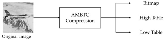
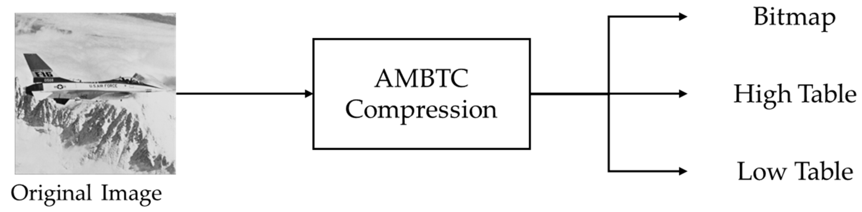
The flow of the AMBTC compression phase used in both Chang et al. [19] and Liu et al. [23] is described in Figure 1. Given a $W\times H$ cover image $I$, AMBTC first divides it into non-overlapping $n\times n$ blocks. Each block is compressed into a trio: a bitmap $bm$, a high value $h$, and a low value $l$. Finally, the entire compressed file consists of a complete bitmap $BM$, a high table $HT$, and a low table $LT$.

Figure 1. Flow of AMBTC compression phase.

2.2. Secret Data Embedding

There are different techniques involved in AMBTC secret data embedding. Both [19] and [23] conceal secret data into value tables $HT$ and $LT$ using a JNC scheme. The cover image after embedding confidential data is then represented by ${HT}^{\prime }$ and ${LT}^{\prime }$.

2.2.1. Value Table Embedding Using JNC

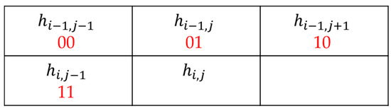
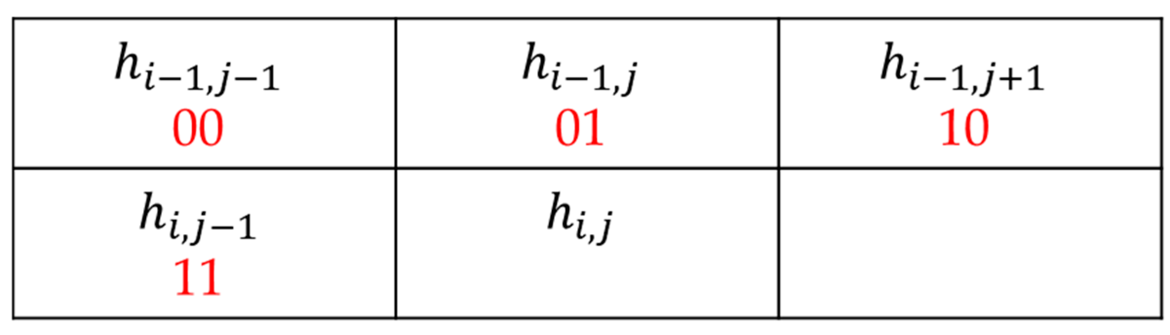
Both refs. [19,23] conceal secret data into the value tables $HT$ and $LT$ sequentially using JNC. The embedding procedure for $HT$ and $LT$ is identical; therefore, we use the secret data embedding process for $HT$ as an example. The high values located in the first row, first column, and last column of $HT$ are kept unchanged as reference values during the embedding phase. The remaining values in $HT$ are considered embeddable and can be used to embed secret data. For an embeddable value $h_{i,j}$ located at position $(i,j)$ in $HT$, four reference values are shown in Figure 2.

Figure 2. Four reference values of $h_{i,j}$ and their corresponding codes.

The embedding steps of a high value through JNC is described below:

• Obtain two bits s₁, s₂ from the binary secret S and find the reference value $h_s$ for $h_{i,j}$ based on Figure 2.
• Calculate the difference e between the current value $h_{i,j}$ and its reference value $h_s$using the XOR operation:

  $$e=h_{i,j}⨁h_s.$$

  (1)
• Set the category index based on the difference e according to:

  $$E=\left\{\begin{array}{c}00,\\ 01,\\ \begin{array}{c}10,\\ 11,\end{array}\end{array} \right.\begin{array}{c}\begin{array}{c} \mathrm{i}\mathrm{f} e\in \left[\mathrm{0,7}\right]\\ \mathrm{i}\mathrm{f} e\in \left[\mathrm{8,15}\right]\end{array}\\ \begin{array}{c} \mathrm{i}\mathrm{f} e\in \left[\mathrm{16,31}\right]\\ \mathrm{o}\mathrm{t}\mathrm{h}\mathrm{e}\mathrm{r}\mathrm{w}\mathrm{i}\mathrm{s}\mathrm{e}\end{array}\end{array}.$$

  (2)
• Set stego high value $h_{i,j}^{\prime }$ to $s_1\parallel s_2\parallel E$ initially, where the notation “$\left|\right|$” represents the concatenation operation. The $h_{i,j}^{\prime }$ is then generated according to the value of E.

  4.1

  When E is 00, use $e^3$ to indicate that 3 bits are needed to represent the value e and can embed 5 bits $s^5$ from S. Then, concatenate e³ and $s^5$ into the initial $h_{i,j}^{\prime }$ to obtain the final stego value, i.e., $h_{i,j}^{\prime }=s_1\parallel s_2\parallel E\parallel e^3\parallel s^5$.

  4.2

  When E is 01, ${\left(e-8\right)}^3$ is used to indicate that the value of (e$-$8) needs 3 bits to represent, and can embed 5 bits s⁵ from S as well. Then, concatenate (e$-$8)³ and $s^5$ into the initial $h_{i,j}^{\prime }$ to obtain the final stego value, i.e., $h_{i,j}^{\prime }=s_1\parallel s_2\parallel E\parallel {\left(e-8\right)}^3\parallel s^5$.

  4.3

  When E is 10, ${\left(e-16\right)}^4$ requires 4 bits to represent the value of (e$-$16) and thus only 4 bits s⁴ from S can be embedded. Then, concatenate (e$-$16)⁴ and s⁴ into $h_{i,j}^{\prime }$ to obtain the final stego value, i.e., $h_{i,j}^{\prime }=s_1\parallel s_2\parallel E\parallel {\left(e-16\right)}^4\parallel s^4$.

  4.4

  Otherwise, $e^8$ is used to indicate that 8 bits are needed to represent the value e. It concatenates $e^8$ into $h_{i,j}^{\prime }$ to obtain the final stego value without secret bit embedding, i.e., $h_{i,j}^{\prime }=s_1\parallel s_2\parallel E\parallel e^8$.

• Output the result $h_{i,j}^{\prime }$.

After every high value $h_{i,j}$ is converted into $h_{i,j}^{\prime }$, all stego high values are converted to their binary forms and concatenated to obtain the stego high table ${HT}^{\prime }$. For a 512 × 512 grayscale image, it needs 8 bits to represent a reference high value. Thus, the total length of the binary forms representing the reference high values is $8\times \left(W+2\times \left(H-1\right)\right)$ and these binary forms are inserted at the front of ${HT}^{\prime }$.

The stego low list ${LT}^{\prime }$ is obtained by employing the same principle.

2.2.2. Bitmap Embedding Using SM

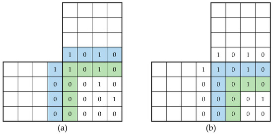
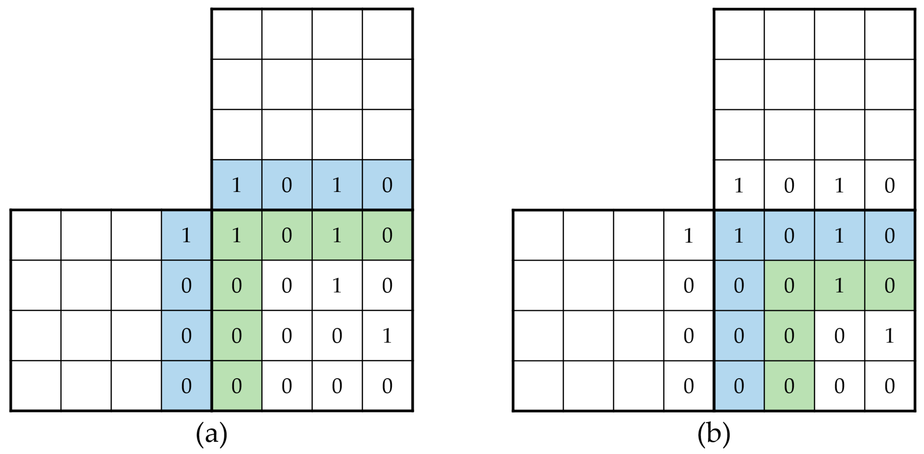
In [23], secret data are concealed into bit maps using the SM technique besides the value table embeddings. The two-layer SM embedding process is demonstrated in Figure 3.

Figure 3. The multi-layer SM bitmap embedding. (a) The first layer. (b) The second layer.

The process of the multi embedding layers for the $n\times n$ bitmap is described as followings:

• During the first layer of bitmap embedding, the bits in the current bitmap adjacent to its left and upper neighboring bitmaps are selected for order permutations. These bits are collected as shown in the green area of Figure 3a. The total number of distinct permutations for the $n\times n$ bitmap ${bm}_{ij}$in the pass $p$ can be calculated as

  $$P_l=\left({\displaystyle \genfrac{}{}{0pt}{}{2\left(n-\left(p-1\right)\right)-1}{bc\left(0\right), bc\left(1\right)}}\right)={\displaystyle \frac{2\left(n-\left(p-1\right)\right)-1!}{bc\left(0\right)!bc\left(1\right)!}}.$$

  (3)

It uses the uniqueness of the Euclidean distance between the neighboring bits and current process bits to determine if the layer is embeddable or not. When the distance is a unique minimum distance, the pass is embeddable; otherwise, it is non-embeddable. An extra bit stream is added for these embedding indicators.

2.

As for the second layer and onward, it is the same process as the first one used but the number of bits involved in the permutation is decreased to $\left(n-1\right)\times (n-1)$, where $p$ is the current pass. Another exception is that the upper neighboring bits and the left neighboring bits are in the same block not its upper and left blocks.

3.

After the bitmap $bm$ is embedded, a stego bitmap ${bm}^{\prime }$ is generated.

Finally, all stego bitmaps are collected to form ${BM}^{\prime }$. Secret data are embedded into bitmaps to increase the embedding capacity of the AMBTC trio.

2.3. Secret Data Extraction and Image Reconstruction

The receiver, after receiving the ${BM}^{\prime }$, ${HT}^{\prime }$, and ${LT}^{\prime }$, can extract the embedded confidential data and retrieve the AMBTC decompressed image. Based on the reconstructed $BM$, $HT$, and $LT$, the AMBTC uncompressed image $I^{\prime }$ can be reconstructed by a block manner. The pixels in a block $B^{\prime }$ of $I^{\prime }$ can be reconstructed after retrieving a bit map bm from $BM$, a high value h and a low value l from the $HT$ and $LT$ value tables. After reconstructing all blocks, the decompressed image $I^{\prime }$ can be obtained.

2.3.1. Value Table Extraction and Reconstruction

Since extracting $HT$ from ${HT}^{\prime }$ is exactly the same process as extracting $LT$ from ${LT}^{\prime }$, we take the extraction of $HT$ as an example. Since the high values located at the first row, the first column, and the last column in $HT$ are for references, the reference high values are reconstructed by extracting the first $8\times \left(W+2\times \left(H-1\right)\right)$ bits from ${HT}^{\prime }$. Then, extract every 12 bits from ${HT}^{\prime }$ as a stego high value. Travel these stego high values from top to bottom, left to right to extract the embedded secret data and recoup the cover high value. The detail of secret data extraction and high value reconstruction is shown in the following steps:

• Convert the stego high value $h_{i,j}^{\prime }$ to its binary form.
• Extract two bits s₁, s₂ from $h_{i,j}^{\prime }$ and consider them as the code to determine the reference value $h_s$ by looking at Figure 2. The embedded secret data S = {s₁, s₂}₂ are extracted.
• Extract another two bits $E^{\prime }$ from $h_{i,j}^{\prime }$. The difference e and the embedded secret data can be retrieved by the value of $E^{\prime }$.

  3.1

  If $E^{\prime }$ equals to 00. Extract 3 bits from $h_{i,j}^{\prime }$ and convert them into a digit value e. The last 5 bits s⁵ in $h_{i,j}^{\prime }$ is the embedded secret data. Thus, the embedded secret data S = {s₁, s₂, 1, 1, s⁵}₂.

  3.2

  If $E^{\prime }$ equals to 01. In this case, we also retrieve 3 bits from $h_{i,j}^{\prime }$ and convert them into a digit value $e^{\prime }$ and e is set as $\left(e^{\prime }+8\right)$. The last 5 bits s⁵ in $h_{i,j}^{\prime }$ is the embedded secret data. Thus, the embedded secret data S = {s₁, s₂, 1, 0, s⁵}₂.

  3.3

  If $E^{\prime }$ equals to 10. In this case, we retrieve 4 bits from $h_{i,j}^{\prime }$ and convert them into a digit value $e^{\prime }$ and e is set as $\left(e^{\prime }+16\right)$. The last 4 bits s⁴ in $h_{i,j}^{\prime }$ is the embedded secret data. Thus, the embedded secret data S = {s₁, s₂, 0, 1, s⁴}₂.

  3.4

  Otherwise, no secret data embedded in this case, and convert last 8 bits e⁸ in $h_{i,j}^{\prime }$ into a digit value e. Thus, the embedded secret data S = {s₁, s₂, 0, 0}₂.

• After retrieving the value of e, the cover high value $h_{i,j}$ can be gained by

  $$h_{i,j}=e⨁h_s.$$

  (4)
• Return $h_{i,j}$ and the embedded secret data S.

After processing all stego high values, the high table $HT$ is reconstructed. By using the same processing, the low table $LT$ is reconstructed as well. At the same time, the embedded secret data can be retrieved correctly.

2.3.2. Bitmap Extraction and Reconstruction

The bits in the top row and the leftmost column of a stego bitmap are kept unmodified during embedding. These bits are used as the restoration references during the side-matching reconstruction process. The same as the embedding, extraction is a multi-pass process corresponding to its embedding process. The bits in the current bitmap are selected the same way during the multi-pass process to generate related permutation tables. In order to reconstruct the bitmaps, the side-match technique is applied during the reconstruction stage as well. In each pass, find the shortest Euclidean distance to reconstruct bits in the bitmap and extract the embedded data.

3. Proposed Scheme

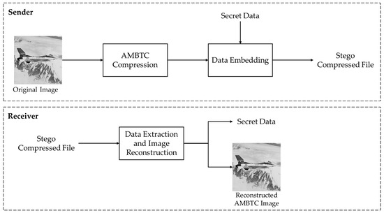
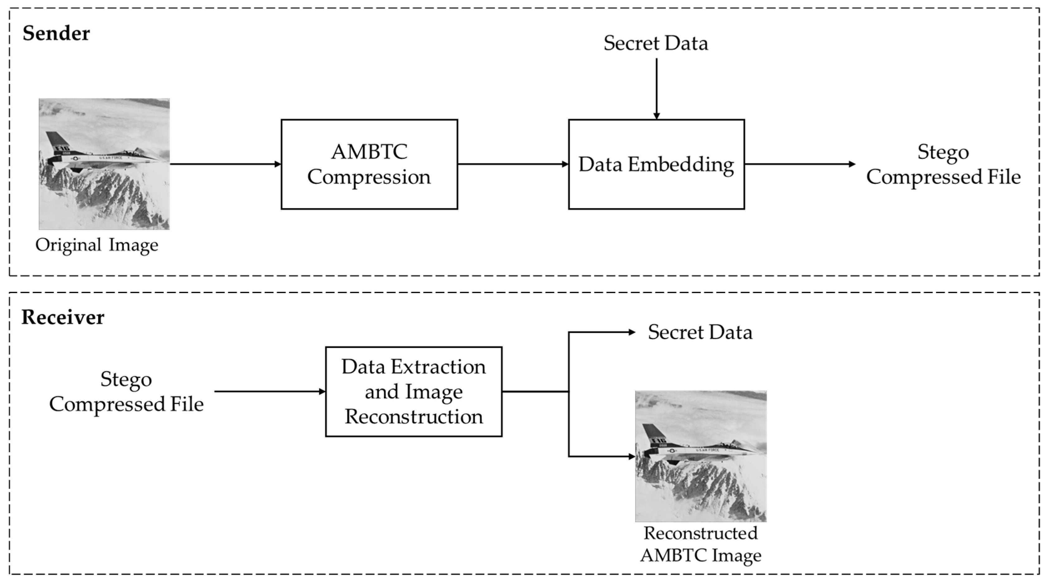
The sender first compresses the original AMBTC image and embeds the secret data into the compressed file, producing a stego compressed file. Upon receiving the stego compressed file, the receiver can extract the secret data and reconstruct the AMBTC image reversibly. Figure 4 illustrates the flow of the proposed scheme.

Figure 4. Flow of our proposed scheme.

3.1. AMBTC Compression Phase

We use the AMBTC compression algorithm described in Section 2.1 of Related Work. For each block, the algorithm generates an 8-bit high value, an 8-bit low value, and a 16-bit bitmap. As an additional preprocessing step, shown in Equation (5), we calculate the difference between the high value and the low value using arithmetical differential coding. Here, $h$ denotes the high value, $l$ denotes the low value, and $d$ denotes the difference. After processing all the blocks, we obtain a high table, a low table, a difference table, and a bitmap table.

$$d=h-l.$$

(5)

3.2. Data Embedding Phase

The proposed scheme embeds data in two stages. The high table, the low table, and the difference table are considered as value tables. For a value table, logical differential coding is used to embed data. The combination of two value tables is selected based on the largest embedding capacity obtained. Bitmap embeddings are mainly based on the side match algorithm. After two layers of SM embeddings, a third layer of embedding is performed by applying Huffman coding compression to unprocessed bits in the bitmap to create space for embedding data.

(1)

Embed Data into Value Tables

Algorithm 1 describes the process of embedding data into the value table in detail. First, the JNC algorithm is used to conceal data into the high table $HT$, the low table $LT$, and the difference table $DT$, respectively. The first row, the first column, and the last column of a value table are reserved as references and their original values are maintained. For the remaining positions, the XOR value $e_{ij}$ of the current value and the reference value, selected based on a 2-bit secret, is calculated. Due to the inherent properties of the XOR operation, boundary pixels are immune to both overflow and underflow issues. Depending on the magnitude of $e_{ij}$, $E_{ij}$ is used as a category indicator and the secret embedding capacity ${EC}_{ij}$ is then determined. After traversing all positions, the embedding capacities of the three tables are obtained. There are three possible combinations of the value tables: $HT$ and $LT$, $HT$ and $DT$, and $LT$ and $DT$. To distinguish the three combinations, the table indicators 00, 01, and 1 are used, respectively. The table combination with the largest embedding capacity is selected for data storage. Finally, the value table encoding stream $VTES$ is generated and output according to the JNC algorithm.

Algorithm 1 Embed Data into Value Tables
Input	High table $HT$, low table $LT$, difference table $DT$, secret data $S$.
Output	Value table encoding stream $VTES$.
Step 1	$VTES=\left[\right]$; ${EC}_H=0$; ${EC}_L=0$; ${EC}_D=0$; $k=0$; $[row, col]=sizeof\left(HT\right)$;
Step 2	for $i$ = 2:$row$   for $j$ = 2:$col-$1    ${rp}_{Hij}=get\_reference\_pixel(HT,i,j)$    $p_{Hij}=HT(i,j)$;    $e_{Hij}=p_{Hij}\oplus {rp}_{Hij}$;    $[E_{Hij}, {{bin}_e}_{Hij}, {EC}_H]=process\_encoding(e_{Hij}, {EC}_H)$;    ${rp}_{Lij}=get\_encoded\_pixel(LT,i,j)$    $p_{Lij}=LT(i,j)$;    $e_{Lij}=p_{Lij}\oplus {rp}_{Lij}$;    $[E_{Lij}, {{bin}_e}_{Lij}, {EC}_L]=process\_encoding(e_{Lij}, {EC}_L)$;    ${rp}_{Dij}=get\_reference\_pixel(DT,i,j)$    $p_{Dij}=DT(i,j)$;    $e_{Dij}=p_{Dij}\oplus {rp}_{Dij}$;    $[E_{Dij}, {{bin}_e}_{Dij}, {EC}_D]=process\_encoding(e_{Dij}, {EC}_D)$;  end for end for
	function $rp=get\_reference\_pixel(table, i, j)$   switch $S(k:k+1)$    case ‘00’     $rp=table(i-1, j-1)$;    case ‘01’     $rp=table(i-1, j)$;    case ‘10’     $rp=table(i-1, j+1)$;    case ‘11’     $rp=table(i, j-1)$;  end switch   $k=k+2$; end function
	function $[E_{ij}, {{bin}_e}_{ij}, EC]=process\_encoding(e_{ij}, EC)$   if $e_{ij}\le 7$    $E_{ij}$ = ‘00’;    ${{bin}_e}_{ij}=dec2bin\left(e_{ij}\right)$;    ${EC}_{ij}=5$;   elseif $e_{ij}\le 15$    $E_{ij}$ = ‘01’;    ${{bin}_e}_{ij}=dec2bin(e_{ij}-8)$;    ${EC}_{ij}=5$;   elseif $e_{ij}\le 31$    $E_{ij}$ = ‘10’;    ${{bin}_e}_{ij}=dec2bin(e_{ij}-16)$;    ${EC}_{ij}=4$;   else    $E_{ij}$ = ‘11’;    ${{bin}_e}_{ij}=dec2bin\left(e_{ij}\right)$;    ${EC}_{ij}=0$;   end if   $EC=EC+{EC}_{ij}$; end function
Step 3	${EC}_{HL}={EC}_H+{EC}_L$; ${EC}_{HD}={EC}_H+{EC}_D$; ${EC}_{LD}={EC}_L+{EC}_D$; $[{EC}_{max}, index]=max\left(\right[{EC}_{HL}, {EC}_{HD}, {EC}_{LD}\left]\right)$; switch index   case 1    $indicator=$’00’;    $VTES=value\_table\_encoding(HT,LT)$;   case 2    $indicator=$’01’;    $VTES=value\_table\_encoding(HT,DT)$;   case 3    $indicator=$’1’;    $VTES=value\_table\_encoding(LT,DT)$; end switch
	function $VTES=value\_table\_encoding({table}_1,{table}_2)$   $VTES=VTES\left|\right|indicator$;   for $i$ = 1:$row$    for $j$ = 1:$col$     if $i$ == 1 or $j$ == 1      $VTES=VTES\left|\right|dec2bin\left({table}_1\left(i,j\right)\right)$;      $VTES=VTES\left|\right|dec2bin\left({table}_2\left(i,j\right)\right)$;     else      if ${EC}_{{table}_{1}ij} \ne 0$       $VTES=VTES\left|\right|E_{{table}_{1}ij}\left|\right|e_{{table}_{1}ij}\left|\right|S(k:k+{EC}_{{table}_{1}ij}-1)$       $k=k+{EC}_{{table}_{1}ij}$;      end if      if ${EC}_{{table}_{2}ij} \ne 0$       $VTES=VTES\left|\right|E_{{table}_{2}ij}\left|\right|e_{{table}_{2}ij}\left|\right|S(k:k+{EC}_{{table}_{2}ij}-1)$       $k=k+{EC}_{{table}_{2}ij}$;      end if     end if    end for   end for end function
Step 4	Output value table encoding stream $VTES$.

(2)

Embed Data into Bitmap

Algorithm 2 describes the process of embedding secret data into a bitmap $BM$. The bitmap is divided into $4\times 4$ blocks, and three layers of embedding processes are applied to each block. For the first layer of embedding, side match prediction is used to determine the 7 side bits of the current block based on the surrounding blocks. Blocks at the first row and first column are treated as references which are not processed in this layer. For each block, the 7 bits are checked to determine if they are all 0 or all 1. If so, embedding is not possible, and the bit values can be naturally inferred without requiring an indicator. Otherwise, side bits from adjacent blocks are used to predict reference values. All possible bit combinations of the 7 side bits are then generated, and their Euclidean distances from the reference bits are calculated. If the distance of the original 7 side bits is the closest one among all combinations, the block can be embedded. A ‘1’ is marked as an indicator, and secret data bits are embedded. If the distance of the original bits is not the closest one, a ‘0’ is used to indicate that bits are not embeddable. The second layer of embedding is similar to the first one except it focuses on side matching within the block. Here, the 7 side bits within the block are used to predict the 5 bits selected for the second layer embedding. Same as the first layer embedding, the bit combinations are listed and Euclidean distances are calculated. Secret data are embedded in the same manner as in the first layer. As for the third layer of embedding, the $2\times 2$ sub-block at the lower-right corner of the $4\times 4$ block is used. These 4 bits, which has not yet been processed, are treated as symbols. After counting the occurrences of these symbols across all blocks, Huffman coding is applied to compress the data. The freed space can then be used to embed additional secret data. Finally, the bitmap encoding stream $BMES$ is generated as the output.

Algorithm 2 Embed Data into Bitmap
Input	Bitmap $BM$, secret data $S$.
Output	Bitmap encoding stream $BMES$.
Step 1	$BMES=\left[\right]$; $indicator=\left[\right]$; ${EC}_{BM}=0$; ${size}_{block}=4$;
Step 2	for $i$ = ${size}_{block}$ + 1:$row$:${size}_{block}$   for $j$ = ${size}_{block}$+1:$col$:${size}_{block}$    $b\left(1\right)=BM\left(i,j\right)$;    $b\left(2\right)=BM\left(i,j+1\right)$;    $b\left(3\right)=BM\left(i,j+2\right)$;    $b\left(4\right)=BM\left(i,j+3\right)$;    $b\left(5\right)=BM\left(i+1,j\right)$;   $b\left(6\right)=BM\left(i+2,j\right)$;    $b\left(7\right)=BM\left(i+3,j\right)$;    if $~(all\left(b==0\right) || all(b==1\left)\right)$     $rb\left(1\right)=ceil\left(\right(BM\left(i-1,j\right)+BM\left(i,j-1\right))/2)$;     $rb\left(2\right)=BM\left(i-1,j+1\right)$;     $rb\left(3\right)=BM\left(i-1,j+2\right)$;     $rb\left(4\right)=BM\left(i-1,j+3\right)$;     $rb\left(5\right)=BM\left(i+1,j-1\right)$;     $rb\left(6\right)=BM\left(i+2,j-1\right)$;     $rb\left(7\right)=BM\left(i+3,j-1\right)$;     $permutations=unique\left(perm\left(b\right)\right);$     $[~, index]=ismember(b,permutations)$;     for $l$ = 1:$size(permutations,2)$      $D\left(l\right)=0$;      for $m$ = 1:7       $D\left(l\right)=D\left(l\right)+(rb\left(m\right)-permutations\left(m,l\right){)}^2;$     end for     end for     $D_{sorted}=sort\left(D\right)$;    if ${index}_{sorted}=1$     ${[b}_{embed}]=data\_embedding(b,S)$;     $BMES=[BMES,b_{embed}]$;      ${EC}_{BM}={EC}_{BM}+floor\left({log}_2\right(size(permutations,2)\left)\right)$;      $indicator=[indicator,‘1’]$;     else     $indicator=[indicator,‘0’]$;     end    end if   end for end for
Step 3	for $i$ = ${size}_{block}$:$row$:${size}_{block}$   for $j$ = ${size}_{block}$:$col$:${size}_{block}$    $b2\left(1\right)=BM\left(i+1,j+1\right)$;    $b2\left(2\right)=BM\left(i+1,j+2\right)$;    $b2\left(3\right)=BM\left(i+1,j+3\right)$;    $b2\left(4\right)=BM\left(i+2,j+1\right)$;    $b2\left(5\right)=BM\left(i+3,j+1\right)$;    if $~(all\left(b2==0\right) || all(b2==1\left)\right)$     $rb2\left(1\right)=ceil\left(\right(BM\left(i,j+1\right)+BM\left(i+1,j\right))/2)$;     $rb2\left(2\right)=BM\left(i,j+2\right)$;     $rb2\left(3\right)=BM\left(i,j+3\right)$;     $rb2\left(4\right)=BM\left(i+2,j\right)$;     $rb2\left(5\right)=BM\left(i+3,j\right)$;     $permutations2=unique\left(perm\left(b2\right)\right);$     $[~, index2]=ismember(b2,permutations2)$;     for $l$ = 1:$size\left(permutations\mathrm{2,2}\right)$      $D2\left(l\right)=0$;      for $m$ = 1:7       $D2\left(l\right)=D2\left(l\right)+(rb2\left(m\right)-permutations2\left(m,l\right))^2;$      end for     end for     ${D2}_{sorted}=sort\left(D2\right)$;     if ${index2}_{sorted}=1$      ${b2}_{embed}=data\_embedding(b2,S)$;      $BMES=[BMES,{b2}_{embed}]$;      ${EC}_{BM}={EC}_{BM}+floor\left({log}_2\right(size\left(permutations\mathrm{2,2}\right)\left)\right)$;      $indicator=[indicator,‘1’]$;     else     $indicator=[indicator,‘0’]$;     end    end if   end for end for
Step 4	$symbols=\left[\right]$; for $i$ = ${size}_{block}$:$row$:${size}_{block}$   for $j$ = ${size}_{block}$:$col$:${size}_{block}$    $b3\left(1\right)=BM\left(i+2,j+2\right)$;    $b3\left(2\right)=BM\left(i+2,j+3\right)$;    $b3\left(3\right)=BM\left(i+3,j+2\right)$;    $b3\left(4\right)=BM\left(i+3,j+3\right)$;    $symbol=[b3\left(1\right), b3\left(2\right), b3\left(3\right), b3\left(4\right)]$;    $symbols=[symbols,symbol]$;   end for end for $[unique\_symbols, ~, idx]=unique\left(symbols\right)$; $frequencies=accumarray(idx, 1)$; $probabilities=frequencies / sum\left(frequencies\right)$; $\left[dict\right]=huffmandict(unique\_symbols, probabilities)$; $encode=\left[huffmanenco\right(symbols, dict)$; ${EC}_{BM}={EC}_{BM}+\left(length\right(symbols)\ast 4-length(encode\left)\right)$; $BMES=[BMES,unique\_symbols,frequencies,encode,S(k:k+{EC}_{BM}\left)\right]$;
Step 5	Output bitmap encoding stream $BMES$.

3.3. Data Extraction and Image Reconstruction

The data extraction and image reconstruction phase are also carried out in two stages. For value tables, we first identify the two stored value tables based on the table indicator. These tables are then decoded not only to restore the original high and low tables but also to extract the secret data. For bitmaps, the first two layers employ side-matching to restore the image and extract the secrets. The third layer extraction uses Huffman decoding to reconstruct the bitmap and retrieve the secret data.

(1)

Reconstruct Value Tables and Extract Data

Algorithm 3 describes the process of reconstructing the value tables and extracting data. The input is the value table encoding stream $VTES$. First, the prefix code is read to obtain the table indicator. The subsequent $VTES$ is then divided into two parts: value table ${VT}_1$ and ${VT}_2$. The first row, the first column and the last column of a value table are used for references. Other than references occupying 8 bits each, the other positions containing embedded data occupy 12 bits each. The value tables ${VT}_1$ and ${VT}_2$ are processed separately but following the same processing steps: select a reference position based on the 2-bit secret data as in the JNC method; then reconstruct the original value using logical differential coding and extract the secret data; use the table indicator to determine which tables are reconstructed. If the table indicator is ‘00’, ${VT}_1$ represents the high table $HT$ and ${VT}_2$ represents the low table $LT$. If the table indicator is ‘01’, ${VT}_1$ represents the high table $HT$ and ${VT}_2$ represents the difference table $DT$. If the table indicator is ‘1’, ${VT}_1$ represents the low table $LT$ and ${VT}_2$ represents the difference table $DT$. Finally, $HT$ and $LT$ are calculated and reconstructed using arithmetical differential coding.

Algorithm 3 Reconstruct Value Tables and Extract Data
Input	Value table encoding stream $VTES$.
Output	High table $HT$, low table $LT$, secret data $S$.
Step 1	$S=\left[\right]$; $l=1$; $indicator=VTES\left(l\right)$; $l=l+1$; if $indicator$ == ‘0’   $indicator=VTES(l:l+1)$;   $l=l+1$; end if ${VT}_1=VTES(l:l+\left(row+col-1\right)\ast 8+\left(row-1\right)\ast \left(col-1\right)\ast 12$; $l=l+\left(row+col-1\right)\ast 8+\left(row-1\right)\ast \left(col-1\right)\ast 12$; ${VT}_2=VTES(l:l+\left(row+col-1\right)\ast 8+\left(row-1\right)\ast \left(col-1\right)\ast 12$; $l=l+\left(row+col-1\right)\ast 8+\left(row-1\right)\ast \left(col-1\right)\ast 12$;
Step 2	for $i$ = 2:$row$   for $j$ = 2:$col$-1    $tableBits1={VT}_1\left(i,j\right)$;    $[{rp}_{1ij},S]=get\_reference\_pixel\left(tableBits1\right)$;    $[e_{1ij},S]=process\_decoding\left(tableBits1\right)$;    $p_{1ij}=e_{1ij}\oplus {rp}_{1ij}$;    $tableBits2={VT}_2\left(i,j\right)$;    $[{rp}_{2ij},S]=get\_reference\_pixel\left(tableBits2\right)$;    $[e_{2ij},S]=process\_decoding\left(tableBits2\right)$;    $p_{2ij}=e_{2ij}\oplus {rp}_{2ij}$;   end for end for
	function $[rp,S]=get\_reference\_pixel\left(tableBits\right)$   switch $tableBits(1:2)$    case ‘00’     $rp=table(i-1, j-1)$;    case ‘01’     $rp=table(i-1, j)$;    case ‘10’     $rp=table(i-1, j+1)$;    case ‘11’     $rp=table(i, j-1)$;    end switch    $S=[S,tableBits\left(1:2\right)]$; end function
	function $[e_{ij},S]=process\_decoding\left(tableBits\right)$   $E_{ij}=tableBits\left(\mathrm{3,4}\right)$;   if $E_{ij}$ = ‘00’    ${{bin}_e}_{ij}=tableBits(5:7)$;    $e_{ij}=bin2dec\left({{bin}_e}_{ij}\right)$;    $S=[S,tableBits(\mathrm{8,12}\left)\right]$;   elseif $E_{ij}$ = ‘01’    ${{bin}_e}_{ij}=tableBits(5:7)$;    $e_{ij}=8+bin2dec\left({{bin}_e}_{ij}\right)$;    $S=[S,tableBits(\mathrm{8,12}\left)\right]$;   elseif $E_{ij}$ = ‘10’    ${{bin}_e}_{ij}=tableBits(5:8)$;    $e_{ij}=16+bin2dec\left({{bin}_e}_{ij}\right)$;    $S=[S,tableBits(\mathrm{9,12}\left)\right]$;   elseif $E_{ij}$ = ‘11’    ${{bin}_e}_{ij}=tableBits(5:12)$;    $e_{ij}=bin2dec\left({{bin}_e}_{ij}\right)$;   end if end function
Step 3	if $indicator$ == ‘00’   $HT={VT}_1$;   $LT={VT}_2$; else if $indicator$ == ‘01’   $HT={VT}_1$;   $LT={VT}_1-{VT}_2$; else if $indicator$ == ‘1’   $HT={VT}_1+{VT}_2$;   $LT={VT}_1$; end if
Step 4	Output high table $HT$, low table $LT$, secret data $S$.

(2)

Reconstruct Bitmap and Extract Data

Algorithm 4 describes the process of reconstructing a bitmap and extracting data. The input is the bitmap encoding stream $BMES$, and the preset block size is 4. Unlike the embedding stage, we must reconstruct the third layer first. To begin, symbols and their frequencies are extracted from $BMES$. Next, the Huffman tree is calculated and constructed, followed by decoding the Huffman encoding stream. Once decoding is completed, the symbols are replaced in the bitmap, and part of the secret data is extracted. The reconstruction then proceeds to the first layer. For each block, the 7 bits inside the block are checked. If all bits are 0 or all are 1, it indicates no embedding. Otherwise, a 1-bit embedding indicator is read. If the indicator is ‘1’, it signifies embedding. All possible combinations of the 7 bits are then listed and their Euclidean distances to the corresponding bits derived from adjacent blocks are calculated. The bit combination with the shortest distance is identified as the original 7 side bits from the first layer of embedding, and its binary index represents the secret data. If the indicator is ‘0’, it indicates no embedding, meaning the 7 bits remain unchanged. The second layer is processed similarly to the first layer. First, it is determined whether all bits are 0 or all are 1. If not, the indicator is read, and the shortest Euclidean distance is used for reconstruction and secret data extraction. After processing all three layers, the bitmap is fully reconstructed, and all secret data are successfully extracted.

Algorithm 4 Reconstruct Bitmap and Extract Data
Input	Bitmap encoding stream $BMES$.
Output	Bitmap $BM$, secret data $S$.
Step 1	${size}_{block}=4$; $symbols=\left[\right]$; $probabilities=frequencies / sum\left(frequencies\right)$; $\left[dict\right]=huffmandict(unique\_symbols, probabilities)$; $decode=\left[huffmandeco\right(symbols, dict)$; ${EC}_{BM}={EC}_{BM}+\left(length\right(symbols)\ast 4-length(encode\left)\right)$; $BMES=[BMES,encode,S(k:k+{EC}_{BM}\left)\right]$; for $i$ = ${size}_{block}$:$row$:${size}_{block}$   for $j$ = ${size}_{block}$:$col$:${size}_{block}$    $symbol=symbols(i,j)$;    $BM\left(i+2,j+2\right)=symbol\left(1\right)$;    $BM\left(i+2,j+3\right)=symbol\left(2\right)$;    $BM\left(i+3,j+2\right)=symbol\left(3\right)$;    $BM\left(i+3,j+3\right)=symbol\left(4\right)$;   end for end for $S=[S,{BMES(k:k+EC}_{BM})]$;
Step 2	for $i$ = ${size}_{block}$+1:$row$:${size}_{block}$   for $j$ = ${size}_{block}$+1:$col$:${size}_{block}$    $b\left(1\right)=BM\left(i,j\right)$;    $b\left(2\right)=BM\left(i,j+1\right)$;    $b\left(3\right)=BM\left(i,j+2\right)$;    $b\left(4\right)=BM\left(i,j+3\right)$;    $b\left(5\right)=BM\left(i+1,j\right)$;    $b\left(6\right)=BM\left(i+2,j\right)$;    $b\left(7\right)=BM\left(i+3,j\right)$;    if $~(all\left(b==0\right) || all(b==1\left)\right)$     $rb\left(1\right)=ceil\left(\right(BM\left(i-1,j\right)+BM\left(i,j-1\right))/2)$;     $rb\left(2\right)=BM\left(i-1,j+1\right)$;     $rb\left(3\right)=BM\left(i-1,j+2\right)$;     $rb\left(4\right)=BM\left(i-1,j+3\right)$;     $rb\left(5\right)=BM\left(i+1,j-1\right)$;     $rb\left(6\right)=BM\left(i+2,j-1\right)$;     $rb\left(7\right)=BM\left(i+3,j-1\right)$;     $permutations=unique\left(perm\left(b\right)\right);$     $[~, index]=ismember(b,permutations)$;     for $l$ = 1:$size(permutations,2)$      $D\left(l\right)=0$;      for $m$ = 1:7       $D\left(l\right)=D\left(l\right)+(rb\left(m\right)-permutations\left(m,l\right))^2;$      end for     end for     $D_{sorted}=sort\left(D\right)$;     if $indicator=1$      $S=data\_extraction(b1,S)$;      ${b1}_{reconstructed}=permutations\left({index1}_{sorted}\right)$;      $BM\left(i,j\right)={b1}_{reconstructed}\left(1\right)$;      $BM\left(i,j+1\right)={b1}_{reconstructed}\left(2\right)$;      $BM\left(i,j+2\right)={b1}_{reconstructed}\left(3\right)$;      $BM\left(i,j+3\right)={b1}_{reconstructed}\left(4\right)$;      $BM\left(i+1,j\right)={b1}_{reconstructed}\left(5\right)$;      $BM\left(i+2,j\right)={b1}_{reconstructed}\left(6\right)$;      $BM\left(i+3,j\right)={b1}_{reconstructed}\left(7\right)$;     end    end if   end for end for
Step 3	for $i$ = ${size}_{block}$:$row$:${size}_{block}$   for $j$ = ${size}_{block}$:$col$:${size}_{block}$    $b2\left(1\right)=BM\left(i+1,j+1\right)$;    $b2\left(2\right)=BM\left(i+1,j+2\right)$;    $b2\left(3\right)=BM\left(i+1,j+3\right)$;    $b2\left(4\right)=BM\left(i+2,j+1\right)$;    $b2\left(5\right)=BM\left(i+3,j+1\right)$;    if $~(all\left(b2==0\right) || all(b2==1\left)\right)$     $rb2\left(1\right)=ceil\left(\right(BM\left(i,j+1\right)+BM\left(i+1,j\right))/2)$;     $rb2\left(2\right)=BM\left(i,j+2\right)$;     $rb2\left(3\right)=BM\left(i,j+3\right)$;     $rb2\left(4\right)=BM\left(i+2,j\right)$;     $rb2\left(5\right)=BM\left(i+3,j\right)$;     $permutations2=unique\left(perm\left(b2\right)\right);$     $[~, index2]=ismember(b2,permutations2)$;     for $l$ = 1:$size\left(permutations\mathrm{2,2}\right)$      $D2\left(l\right)=0$;      for $m$ = 1:7       $D2\left(l\right)=D2\left(l\right)+(rb2\left(m\right)-permutations2\left(m,l\right))^2;$      end for     end for     ${D2}_{sorted}=sort\left(D2\right)$;     if $indicator=1$      $S=data\_extraction(b2,S)$;      ${b2}_{reconstructed}=permutations\left({index2}_{sorted}\right)$;      $BM\left(i+1,j+1\right)={b2}_{reconstructed}\left(1\right)$;      $BM\left(i+1,j+2\right)={b2}_{reconstructed}\left(2\right)$;      $BM\left(i+1,j+3\right)={b2}_{reconstructed}\left(3\right)$;      $BM\left(i+2,j+1\right)={b2}_{reconstructed}\left(4\right)$;      $BM\left(i+3,j+1\right)={b2}_{reconstructed}\left(5\right)$;     end    end if   end for end for
Step 4	Bitmap $BM$, secret data $S$.

After the two stages, we obtain the high table, low table, and bitmap, and reconstruct the image using the AMBTC algorithm. By combining the secret data from both stages, the complete secret data can be retrieved.

4. Experimental Results

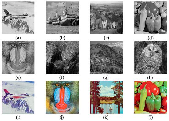
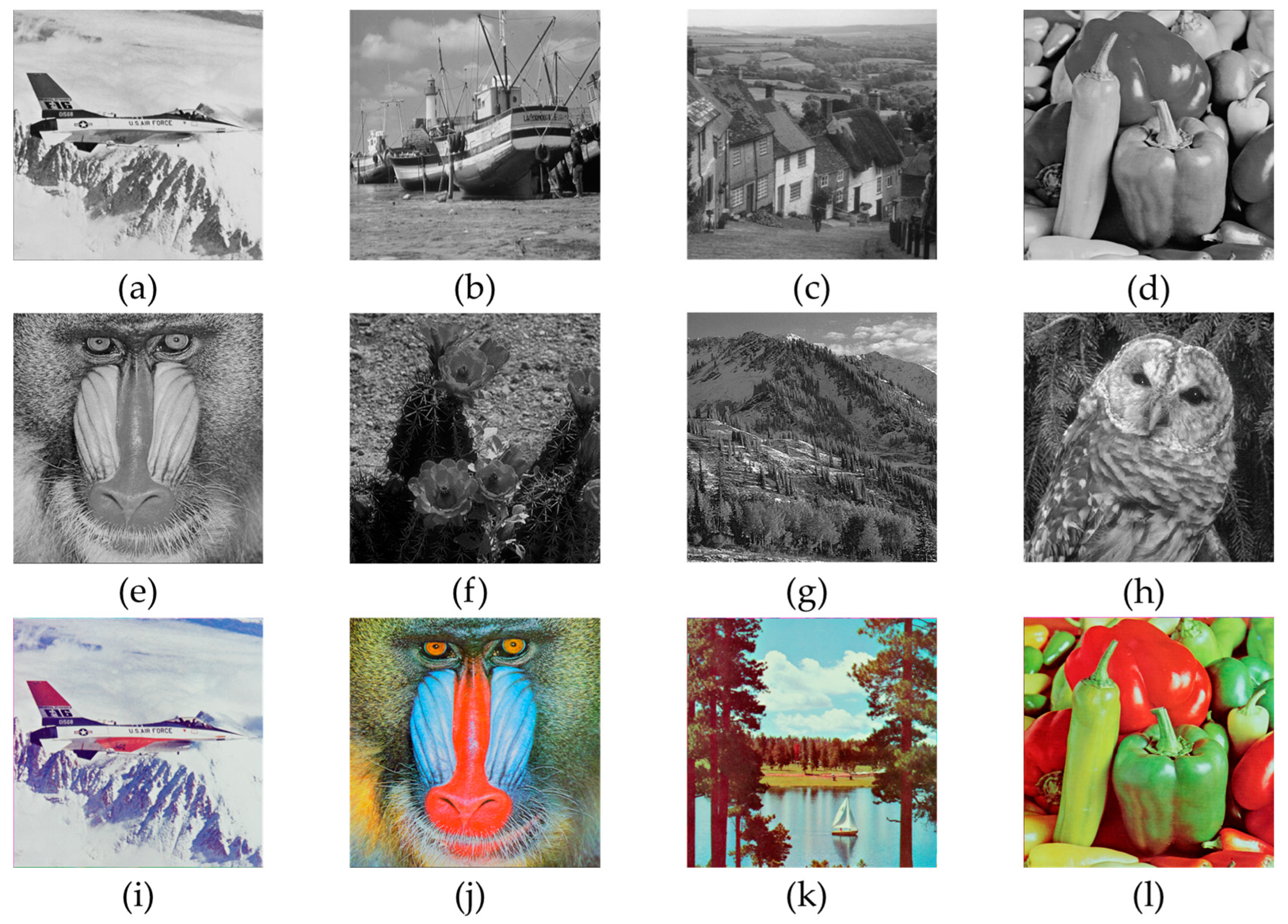
In this section, we present the experimental analysis and compare our results with the most advanced AMBTC data hiding scheme. The experiments were conducted on a Windows 11 computer equipped with a 3.20 GHz AMD Ryzen 7 CPU (AMD, located in Santa Clara, CA, USA) and 16 GB of RAM, using MATLAB 2024a. Figure 5 illustrates the test images used in our scheme. Specifically, the first row represents standard grayscale images, the second row represents complex grayscale images, and the third row represents color images.

Figure 5. Test images: (a–d) standard grayscale images; (e–h) complex grayscale images; (i–l) color images.

The quality of a decompressed image is evaluated using the peak signal-to-noise ratio (PSNR), which quantifies the difference between the original image and the AMBTC decompressed image. The mean square error (MSE), which measures the average squared difference between corresponding pixel values in the original and decompressed images, is used in the calculation of PSNR. In Equations (6) and (7), $I_{ij}$ and $I_{ij}^{\prime }$ represent the corresponding pixel values of the original image and the decompressed image, respectively, while $H$ and $W$ denote the height and width of the images.

$$PSNR=10{\mathit{log}}_{10}\left({\displaystyle \frac{{255}^2}{MSE}}\right),$$

(6)

$$MSE={\displaystyle \frac{\sum _{i=1}^H\sum _{j=1}^W{\left(I_{ij}-I_{ij}^{\prime }\right)}^2}{H\times W}}.$$

(7)

To evaluate the embedding capability, we use two indicators, as shown in Equations (8) and (9). Equation (8) represents the embedding rate (ER), which is calculated by dividing the embedding capacity (EC) by the file size (FS). Equation (9) represents the pure embedding capacity (PEC), which is the embedding capacity reduced by the difference between the file size and the original file size (OFS).

$$ER={\displaystyle \frac{EC}{FS}},$$

(8)

$$PEC=EC-\left(FS-OFS\right).$$

(9)

Table 1 presents a performance comparison of our schemes applied to standard grayscale images. It can be observed that all the schemes are reversible for AMBTC compressed images, resulting in identical PSNR values. The ER of our proposed scheme exceeds 30%. Compared to the scheme proposed by Liu et al. [23] in 2024, our ER is approximately 2% higher, and the PEC is about 15,000 bits greater. Furthermore, it also outperforms other schemes and achieves the best ER and PEC among all.

Table 1. Performance comparison on standard grayscale images with other schemes.

Scheme	Performance	Airplane	Boat	Goldhill	Peppers
Sun et al.’s [22]	PSNR	33.292	31.164	33.724	34.102
	FS	530,856	549,620	550,088	538,968
	EC	64,008	64,008	64,008	64,008
	ER	12.06%	11.65%	11.64%	11.88%
	PEC	57,440	38,676	38,208	49,328
Chang et al.’s [25]	PSNR	33.292	31.164	33.724	34.102
	FS	524,288	524,288	524,288	524,288
	EC	4640	2245	2119	3137
	ER	0.89%	0.43%	0.40%	0.60%
	PEC	4640	2245	2119	3137
Lin et al.’s [17]	PSNR	33.292	31.164	33.724	34.102
	FS	1,042,312	1,044,800	1,044,536	1,044,720
	EC	262,016	262,144	261,968	262,144
	ER	25.14%	25.09%	25.08%	25.09%
	PEC	−256,008	−258,368	−258,280	−258,288
Chang et al.’s [19]	PSNR	33.292	31.164	33.724	34.102
	FS	652,304	652,304	652,304	652,304
	EC	177,814	166,786	168,185	174,222
	ER	27.26%	25.57%	25.78%	26.71%
	PEC	49,798	38,770	40,169	46,206
Liu et al.’s [23]	PSNR	33.292	31.164	33.724	34.102
	FS	664,985	666,583	667,206	666,234
	EC	202,772	189,805	196,618	191,705
	ER	30.49%	28.47%	29.47%	28.77%
	PEC	62,075	47,510	53,700	49,759
Proposed	PSNR	33.292	31.164	33.724	34.102
	FS	664,987	666,585	667,207	666,236
	EC	218,569	204,514	216,122	207,605
	ER	32.87%	30.68%	32.39%	31.16%
	PEC	77,870	62,217	73,203	65,657

Table 2 presents a performance comparison of our schemes on complex grayscale images. It can be observed that the PSNR is slightly lower for complex grayscale images. Due to the relatively low correlation within image blocks, the EC is also reduced, leading to lower ER and PEC compared to standard grayscale images. Nevertheless, our scheme still achieves the best results compared to other schemes. The image ‘Owl’ performs particularly well, with embedding rate reaching 28.88% and a PEC of 49,726.

Table 2. Performance comparison on complex grayscale images with other schemes.

Scheme	Performance	Baboon	Flowers	Mountain	Owl
Chang et al.’s [19]	PSNR	27.782	27.498	25.145	30.011
	FS	652,304	652,304	652,304	652,304
	EC	151,439	148,275	144705	144,497
	ER	23.22%	22.73%	22.18%	22.15%
	PEC	23,423	20,259	16,689	16,481
Liu et al.’s [23]	PSNR	27.782	27.498	25.145	30.011
	FS	667,264	667,076	667,087	667,283
	EC	170,653	165,722	165,964	170,484
	ER	25.58%	24.84%	24.88%	25.55%
	PEC	27,677	22,934	23,165	27,489
Proposed	PSNR	27.782	27.498	25.145	30.011
	FS	667,265	667,077	667,088	667,284
	EC	182,992	178,214	174,173	192,722
	ER	27.42%	26.72%	26.11%	28.88%
	PEC	40,015	35,425	31,373	49,726

Table 3 presents a performance comparison between our schemes and other schemes on color images. Since RGB images have three channels, their file size is typically about three times larger than that of grayscale images. It can be observed that our proposed scheme demonstrates superior embedding ability while maintaining an almost identical file size to other schemes. For the color image ‘Airplane’, the embedding rate reaches 32.87%, and the PEC achieves 233,726 bits. It represents a significant improvement over other schemes.

Table 3. Performance comparison on color images with other schemes.

Scheme	Performance	Airplane	Baboon	Lake	Peppers
Chang et al.’s [19]	PSNR	32.443	26.381	29.2895	32.730
	FS	1,956,912	1,956,912	1,956,912	1,956,912
	EC	546,265	442,252	496,115	531,092
	ER	27.91%	22.60%	25.35%	27.14%
	PEC	162,217	58,204	112,067	147,044
Liu et al.’s [23]	PSNR	32.443	26.381	29.2895	32.730
	FS	1,994,889	2,001,775	2,000,304	1,998,469
	EC	614,088	495,377	546,542	573,364
	ER	30.78%	24.75%	27.32%	28.69%
	PEC	192,063	66,466	119,102	147,759
Proposed	PSNR	32.443	26.381	29.2895	32.730
	FS	1,994,895	2,001,778	2,000,307	1,998,473
	EC	655,757	529,582	580,605	617,448
	ER	32.87%	26.46%	29.03%	30.90%
	PEC	233,726	100,668	153,162	191,839

We also evaluated the performance on different image sizes. Experiments were conducted on three sizes of the grayscale image ‘Airplane’: 256 × 256, 512 × 512, and 1024 × 1024. As shown in Table 4, the embedding performance of our proposed scheme is superior to other schemes across all three sizes, particularly for the 1024 × 1024 image, where the ER and PEC reach 40.00% and 491,892 bits, respectively.

Table 4. Performance comparison on the image ‘Airplane’ of different sizes with other schemes.

Scheme	Performance	256 × 256	512 × 512	1024 × 1024
Chang et al.’s [19]	PSNR	29.655	33.292	35.889
	FS	162,320	652,304	2,615,312
	EC	41,210	177,814	761,248
	ER	25.39%	27.26%	29.11%
	PEC	9962	49,798	243,088
Liu et al.’s [23]	PSNR	29.655	33.292	35.889
	FS	165,730	664,985	2,675,492
	EC	48,741	202,772	936,456
	ER	29.41%	30.49%	35.00%
	PEC	14,083	62,075	358,116
Proposed	PSNR	29.655	33.292	35.889
	FS	165,732	664,987	2,675,494
	EC	52,785	218,569	1,070,234
	ER	31.85%	32.87%	40.00%
	PEC	18,125	77,870	491,892

To demonstrate the necessity of calculating the difference table based on the value tables, we use the 512 × 512 grayscale image ‘Airplane’ as shown in Table 5. It can be observed that the embedding capacity of the difference table is higher. It suggests that our scheme can outperform the scheme which only uses the high and low tables. Since the embedding capacity of the difference table is the lowest among the three in some cases, we use an additional 2 bits for the table indicator to make sure the highest embedding capacity.

Table 5. Embedding capacity analysis of the value tables on the image ‘Airplane’.

Value Table	EC
High Table	91446
Low Table	87226
Difference Table	95957

Table 6 presents the time complexity of the proposed scheme at different stages. The time complexity for embedding data into a value table, as well as for reconstructing the value table and extracting data, follows a linear complexity, $O\left(n\right)$. In contrast, the time complexity for embedding data into a bitmap, as well as for reconstructing the bitmap and extracting data, is $O(n\times 7\times 7!)$, due to the need to enumerate all permutations of 7 bits in this stage of the process. This increased complexity arises as a trade-off for achieving a higher embedding capacity.

Table 6. Time complexity of the proposed scheme at different stages.

Stage	Time Complexity
Embed Data into Value Table	$O\left(n\right)$
Embed Data into Bitmap	$O(n\times 7\times 7!)$
Reconstruct Value Table and Extract Data	$O\left(n\right)$
Reconstruct Bitmap and Extract Data	$O(n\times 7\times 7!)$

5. Conclusions

This paper proposes a reversible data hiding scheme for AMBTC compressed files. Based on the characteristics of AMBTC compressed files, we perform a two-stage processing of data hiding on the value tables and bitmaps. For the value tables, we introduce a difference table derived from the original high and low tables, which effectively enhances the embedding capacity. For the bitmaps, we further apply Huffman compression as the third layer of embedding building upon the original two-layer side match algorithm. The Huffman compression further frees up additional space for embedding secret data. Experimental results demonstrate that our proposed scheme achieves both higher embedding rates and better pure embedding capacities while maintaining the reversibility of AMBTC compressed files. In the future, we will further explore the carrier characteristics of AMBTC and investigate schemes to find further improvements.

References

- Tian, J. Reversible data embedding using a difference expansion. IEEE Trans. Circuits Syst. Video Technol. 2003, 13, 890–896. [Google Scholar] [CrossRef] [Scilit]
- Alattar, A.M. Reversible watermark using the difference expansion of a generalized integer transform. IEEE Trans. Image Process. 2004, 13, 1147–1156. [Google Scholar] [CrossRef] [Scilit]
- Chan, C.K.; Cheng, L.M. Hiding data in images by simple LSB substitution. Pattern Recognit. 2004, 37, 469–474. [Google Scholar] [CrossRef] [Scilit]
- Ni, Z.; Shi, Y.Q.; Ansari, N.; Su, W. Reversible data hiding. IEEE Trans. Circuits Syst. Video Technol. 2006, 16, 354–362. [Google Scholar]
- Wu, H. Recent advances in reversible watermarking in an encrypted domain. In Advanced Security Solutions for Multimedia; IOP Publishing: Bristol, UK, 2021; pp. 4-1–4-17. [Google Scholar]
- Jiang, X.; Xie, Y.; Zhang, Y.; Ye, Y.; Xu, F.; Li, L.; Su, Y.; Chen, Z. Reversible Data Hiding in Encrypted Images Using Reservoir Computing Based Data Fusion Strategy. IEEE Trans. Circuits Syst. Video Technol. 2024. [Google Scholar] [CrossRef] [Scilit]
- Gao, G.; Yang, S.; Hu, X.; Xia, Z.; Shi, Y.Q. Reversible data hiding-based local contrast enhancement with nonuniform superpixel blocks for medical images. IEEE Trans. Circuits Syst. Video Technol. 2024. [Google Scholar] [CrossRef] [Scilit]
- Linde, Y.; Buzo, A.; Gray, R. An algorithm for vector quantizer design. IEEE Trans. Commun. 1980, 28, 84–95. [Google Scholar] [CrossRef] [Scilit]
- Chavan, P.P.; Sheela Rani, B.; Murugan, M.; Chavan, P. An image compression model via adaptive vector quantization: Hybrid optimization algorithm. Imaging Sci. J. 2020, 68, 259–277. [Google Scholar] [CrossRef] [Scilit]
- Perfilieva, I.; Hurtik, P. The F-transform preprocessing for JPEG strong compression of high-resolution images. Inf. Sci. 2021, 550, 221–238. [Google Scholar] [CrossRef] [Scilit]
- Hamano, G.; Imaizumi, S.; Kiya, H. Effects of jpeg compression on vision transformer image classification for encryption-then-compression images. Sensors 2023, 23, 3400. [Google Scholar] [CrossRef] [Scilit]
- Delp, E.; Mitchell, O. Image compression using block truncation coding. IEEE Trans. Commun. 1979, 27, 1335–1342. [Google Scholar] [CrossRef] [Scilit]
- Yang, C.N.; Chou, Y.C.; Chang, T.K.; Kim, C. An enhanced adaptive block truncation coding with edge quantization scheme. Appl. Sci. 2020, 10, 7340. [Google Scholar] [CrossRef] [Scilit]
- Lin, Y.; Lin, C.C.; Chang, C.C.; Chang, C.C. An IoT-Based Electronic Health Protection Mechanism With AMBTC Compressed Images. IEEE Internet Things J. 2024. [Google Scholar] [CrossRef] [Scilit]
- Lema, M.; Mitchell, O. Absolute moment block truncation coding and its application to color images. IEEE Trans. Commun. 1984, 32, 1148–1157. [Google Scholar] [CrossRef] [Scilit]
- Ou, D.; Sun, W. High payload image steganography with minimum distortion based on absolute moment block truncation coding. Multimed. Tools Appl. 2015, 74, 9117–9139. [Google Scholar] [CrossRef] [Scilit]
- Lin, C.C.; Liu, X.L.; Tai, W.L.; Yuan, S.M. A novel reversible data hiding scheme based on AMBTC compression technique. Multimed. Tools Appl. 2015, 74, 3823–3842. [Google Scholar] [CrossRef] [Scilit]
- Huang, Y.H.; Chang, C.C.; Chen, Y.H. Hybrid secret hiding schemes based on absolute moment block truncation coding. Multimed. Tools Appl. 2017, 76, 6159–6174. [Google Scholar] [CrossRef] [Scilit]
- Chang, C.C.; Chen, T.S.; Wang, Y.K.; Liu, Y. A reversible data hiding scheme based on absolute moment block truncation coding compression using exclusive OR operator. Multimed. Tools Appl. 2018, 77, 9039–9053. [Google Scholar] [CrossRef] [Scilit]
- Kumar, R.; Kim, D.S.; Jung, K.H. Enhanced AMBTC based data hiding method using hamming distance and pixel value differencing. J. Inf. Secur. Appl. 2019, 47, 94–103. [Google Scholar] [CrossRef] [Scilit]
- Horng, J.H.; Chang, C.C.; Li, G.L. Steganography using quotient value differencing and LSB substitution for AMBTC compressed images. IEEE Access 2020, 8, 129347–129358. [Google Scholar] [CrossRef] [Scilit]
- Sun, W.; Lu, Z.M.; Wen, Y.C.; Yu, F.X.; Shen, R.J. High performance reversible data hiding for block truncation coding compressed images. Signal Image Video Process. 2013, 7, 297–306. [Google Scholar] [CrossRef] [Scilit]
- Liu, J.C.; Lin, Y.; Chang, C.C.; Chang, C.C. A side match oriented data hiding based on absolute moment block truncation encoding mechanism with reversibility. Multimed. Tools Appl. 2024, 1–23. [Google Scholar] [CrossRef] [Scilit]
- Wu, D.C.; Tsai, W.H. A steganographic method for images by pixel-value differencing. Pattern Recognit. Lett. 2003, 24, 1613–1626. [Google Scholar] [CrossRef] [Scilit]
- Chang, I.C.; Hu, Y.C.; Chen, W.L.; Lo, C.C. High capacity reversible data hiding scheme based on residual histogram shifting for block truncation coding. Signal Process. 2015, 108, 376–388. [Google Scholar] [CrossRef] [Scilit]
Disclaimer/Publisher’s Note: The statements, opinions and data contained in all publications are solely those of the individual author(s) and contributor(s) and not of MDPI and/or the editor(s). MDPI and/or the editor(s) disclaim responsibility for any injury to people or property resulting from any ideas, methods, instructions or products referred to in the content. |
© 2024 by the authors. Licensee MDPI, Basel, Switzerland. This article is an open access article distributed under the terms and conditions of the Creative Commons Attribution (CC BY) license (https://creativecommons.org/licenses/by/4.0/).