


Abstract
Although numerous studies have developed promising diagnostic algorithms, many have yet to be translated into workflow-integrated tools. Gliomas represent a substantial proportion of primary brain tumors, and their preoperative differentiation by tumor grade can provide critical information for patient management. In this study, we present and evaluate GliomaAI, an open-source 3D Slicer extension for the automated classification of low-grade versus high-grade gliomas from preoperative MRI. The extension is organized into two complementary frameworks for MRI preprocessing and classification with explainability. Four 3D CNN architectures evaluated in our previous work were integrated into a unified segmentation-free workflow, with their final deployment retrained on T1-CE and FLAIR volumes from the multicohort dataset of 1194 patients. GliomaAI offers both individual CNN classification and an ensemble configuration. For single-model predictions, Grad-CAM heatmaps can be interactively overlaid on either MRI volume to aid interpretation of the model’s decision. Explainability is further enhanced through 3D rendering of the generated heatmaps, providing spatial inspection of displayed activations. After excluding overlaps with the model-development cohort, independent validation was conducted on the remaining BraTS-19 cases (26 LGG, 208 HGG). GliomaAI-CNN achieved a balanced accuracy of 82.2% and an AUC of 0.945. The extension provides an accessible, computationally efficient bridge toward clinical application.
1. Introduction
Gliomas represent the most common primary tumors of the Central Nervous System (CNS), accounting for approximately 30% of all primary brain tumors and nearly 80% of malignant brain tumors. According to the World Health Organization (WHO) Classification of CNS Tumors, gliomas are classified into four histopathological grades (G1–4) based on histological features of anaplasia and molecular characteristics. The grade of neoplasms reflects biological aggressiveness, treatment response, and prognosis [1,2,3]. In several computational studies of glioma classification, WHO grades 2 and 3 have been grouped as low-grade gliomas (LGGs), whereas grade 4 tumors have been classified as high-grade gliomas (HGGs), reflecting their markedly more aggressive biological behavior [4,5]. Therefore, accurate preoperative grading is essential for guiding surgical planning, optimizing therapeutic strategies, and improving patient management.
Multiparametric Magnetic Resonance Imaging (MRI) is the standard imaging modality for the non-invasive detection, characterization, and preoperative grading of gliomas [6]. In recent years, the rapid integration of Artificial Intelligence (AI), particularly deep learning, into MRI-based Computer-Aided Diagnosis (CAD) systems has significantly advanced the automated characterization and preoperative classification of gliomas, with the aim of supporting clinical decision-making [7,8]. In particular, three-dimensional (3D) deep learning models applied directly to volumetric MRI have enabled segmentation-independent glioma grading, avoiding the need for labor-intensive manual or error-prone automated tumor delineation [9,10,11].
Translating such glioma grading models into practice, however, depends on the software used to develop and deploy them. Although general-purpose deep learning frameworks, such as TensorFlow [12] and PyTorch [13], facilitate model development, medical imaging requires domain-specific tools that address the particular characteristics of multidimensional clinical data. Frameworks such as MONAI provide standardized components for image preprocessing, model development, inference, and deployment [14]. However, transforming trained models into accessible, readily usable, and task-specific software applications with the potential for clinical integration remains a major challenge [15,16].
In this context, the 3D Slicer platform helps address this challenge by bridging medical image analysis research and the development of practical software tools and applications. 3D Slicer is a free, open-source platform that includes a variety of integrated modules for medical image processing and visualization. Furthermore, its extensible architecture enables researchers and developers to create specialized software tools within the platform [17]. In a recent comparative evaluation of freely available software for medical image analysis research, 3D Slicer ranked among the highest-performing platforms overall, particularly for its broad and customizable functionality [18].
Since software tools targeting glioma grading remain limited, related implementations developed for broader neuro-oncological tasks and other tumor types provide relevant context. Several software tools and 3D Slicer extensions have been developed to facilitate the translation of advanced medical image analysis methods into accessible and reproducible workflows. Among them, the Cancer imaging Phenomics Toolkit (CaPtk) is a standalone platform for oncological imaging that integrates preprocessing, radiomic feature extraction and selection, machine learning analysis, and specialized diagnostic and predictive workflows, including applications for brain tumors [19]. Within the 3D Slicer ecosystem, DeepInfer is an open-source toolkit that enables the integration of trained deep learning models for segmentation and classification tasks through containerized execution. Its public model registry allows researchers to select and apply task-specific models to new data without additional software development or configuration [20].
More specifically, in the field of brain tumor imaging, several 3D Slicer extensions have focused on deep learning-based segmentation using multi-sequence MRI examinations. Slicer-DeepSeg integrates two task-specific pretrained models: DeepSeg, which operates on T2-FLAIR MRI, and nnU-Net, which uses multiple MRI sequences. The extension incorporates automated input preprocessing and enables the resulting glioma segmentations to be visualized in both two-dimensional (2D) slices and three-dimensional (3D) views [21]. More recently, SlicerBatchBrainMRTumorSegmentation has integrated the BraTS Toolkit [22] into 3D Slicer, enabling automated segmentation of multimodal brain MRI data from multiple patients. It provides a user-friendly interface for selecting multiple neural networks and combining their outputs through majority voting or an iterative label-fusion method. The generated segmentations are transformed back into the original MRI space, facilitating visualization and subsequent quantitative analysis [23].
Beyond tumor delineation, 3D Slicer extensions have incorporated classification into broader tumor assessment workflows. RANO2.0-assist supports classification of treatment response in patients with glioblastoma through the comparison of multi-sequence MRI examinations across time points [24]. Similarly, the Breast Ultrasound Analysis uses a pretrained multi-task model to jointly perform breast tumor segmentation and classification [25]. However, in these extensions, classification either depends on information derived from prior tumor extraction or is performed using a model jointly trained for segmentation and classification. Furthermore, neither package integrates explainability features within its interface, even when interpretability analyses are presented in the corresponding manuscripts.
The present study builds upon our previous work [11], adopting its CNN architectures and training methodology. For deployment in GliomaAI, the models were retrained from scratch on the complete development cohort of 1194 patients using High-Performance Computing (HPC) resources, while the present work focuses on their integration into an open-source 3D Slicer workflow and their independent external evaluation.
Against the background described, the main contributions of the present study can be summarized as follows:
- Development of GliomaAI, an open-source and user-friendly 3D Slicer extension providing an automated, segmentation-independent workflow for MRI preprocessing and direct preoperative LGG versus HGG classification from multimodal MRI.
- Deployment of multiple task-specific CNN models, retrained on the complete development cohort for local CPU-based inference on conventional computers, with support for both individual-model and ensemble predictions.
- Integration of Grad-CAM-based explainability directly into the extension, enabling users to examine salient image regions associated with model predictions through adjustable heatmap overlays in 2D slice views and 3D rendering.
- Independent external evaluation of the resulting classification models within the GliomaAI workflow using a separate, non-overlapping subset of the BraTS-19 dataset, assessing classification performance, model configurations, and CPU inference time.
2. Materials and Methods
2.1. GliomaAI Overview and Software Environment
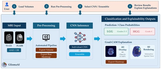
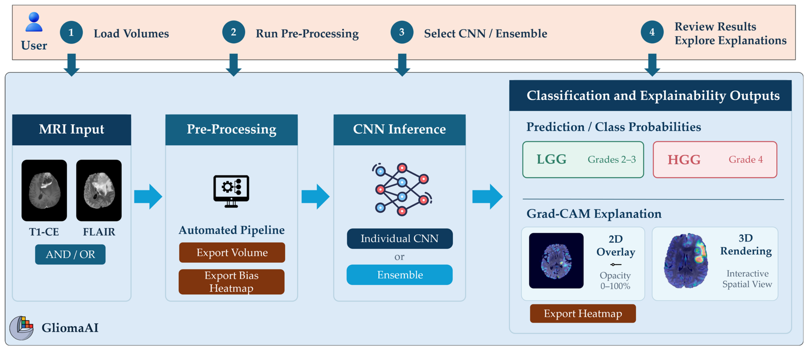
GliomaAI was developed as an open-source scripted module for 3D Slicer, providing an integrated workflow for the automated preprocessing, classification, and explainability analysis of preoperative glioma MRI examinations. The extension accepts as input either one or both T1-weighted contrast-enhanced (T1-CE) and T2-weighted fluid-attenuated inversion recovery (FLAIR) volumes. It provides direct, segmentation-free LGG/HGG classification. Consistent with the labeling scheme adopted in our previous study and with prognostic groupings reported in the recent literature, grade 2 and grade 3 tumors were grouped as LGGs, whereas grade 4 tumors were categorized as HGGs [11,26]. In the context of this study, grade 3 tumors were considered an intermediate-grade category and were included in the LGG class within the binary classification scheme. As discussed in the Introduction, grade 4 tumors represent the highest-grade and most aggressive category and were therefore assigned to the HGG class. The relationship between user-provided inputs, configurable options, and the successive processing stages is summarized schematically in Figure 1.
Figure 1.
Graphical overview of the GliomaAI 3D Slicer extension, illustrating the user-module interaction throughout the main workflow stages and the principal available options.
The integrated workflow combines the preprocessing pipeline with the CNN models developed and evaluated in our previous study [11]. The present work focuses on the development of a friendly Graphical User Interface (GUI) within 3D Slicer that brings these components into a unified environment. The GUI is organized into two main workflows, preprocessing and classification, providing user interaction throughout the analysis process.
GliomaAI was implemented in Python (version 3.10) as a scripted loadable module and packaged as a 3D Slicer extension for installation through the Extensions Manager and subsequent access from the Slicer Modules menu. Version 5.6.2 was used during initial development, and compatibility was subsequently verified with the version 5.12.0. The standard 3D Slicer distribution provides integrated Python environment and the core libraries used for medical image processing, GUI implementation, and visualization. TensorFlow and PyTorch were incorporated as third-party packages to support pretrained CNN inference and Grad-CAM explainability analysis. In addition, the open-source SynthStrip python implementation and its pretrained model weights were installed and retrieved, for automated brain extraction during preprocessing [27]. Table 1 summarizes the additional software dependencies and their respective roles within GliomaAI.
Table 1.
Additional software dependencies and their respective functions within GliomaAI.
All preprocessing, classification, and explainability operations are executed locally within the 3D Slicer environment. Functional and runtime testing was conducted under Windows 11 Home (version 25H2; Microsoft Corporation, Redmond, WA, USA) using an AMD Ryzen 7 250 mobile processor (8 cores, 16 threads, 3.3 GHz base frequency; Santa Clara, CA, USA), 16 GB of RAM, and an NVIDIA GeForce RTX 5050 GPU with 8 GB of VRAM (Santa Clara, CA, USA). The integrated pretrained networks perform CPU-based inference without requiring a dedicated GPU. Missing external packages, including TensorFlow and PyTorch, are installed automatically when required. Model weights that are not bundled with the extension are retrieved on demand from the corresponding GitHub release (v1.0.0). Each set of weights is downloaded only when the corresponding model is first selected by the user, and is verified using SHA-256 checksums before use. If checksum verification fails, the file is downloaded again. An internet connection is required only when a missing dependency must be installed or when a model whose weights are not yet available locally is selected for the first time, but not for subsequent use.
2.2. Graphical User Interface and Visualization Implementation
The GUI was designed using Qt Designer, a rapid and accessible interface-development tool that provides a broad range of interactive widgets [28]. It is available within 3D Slicer and enables visually designed layouts to be stored and integrated into scripted extensions. The GliomaAI interface was organized into two principal tabs corresponding to the preprocessing and classification workflows. User interaction was enabled through selection lists, push buttons, checkboxes, and a slider, allowing the configuration of input volumes, preprocessing operations, CNN models, and explainability visualization settings. These controls were linked to the underlying computational functions responsible for image preprocessing, CNN inference, and Grad-CAM generation.
Within GliomaAI, the input MRI volumes, preprocessing outputs, and Grad-CAM activation maps were managed as volume nodes within Medical Reality Modeling Language (MRML) scene, the core data model of 3D Slicer [17]. Through the Visualization Toolkit (VTK) infrastructure [29], volumes can be interactively inspected in the axial, sagittal and coronal views. Furthermore, the generated explainability heatmaps could be displayed as overlays on the MRI volumes or rendered in 3D for spatial assessment. Classification predictions and probabilities were presented directly within the GUI, allowing the analysis and review of all generated outputs within the same environment.
2.3. Preprocessing Workflow
MRI preprocessing constitutes a central stage of computational medical imaging workflows, particularly for volumetric brain MRI. Acquisitions could differ in a variety of parameters such as orientation, voxel spacing, scanner-dependent intensity distributions, bias-field artifacts, and non-brain tissue content. These sources of heterogeneity can negatively affect AI model performance across diverse downstream tasks, including segmentation, classification, and regression. Preprocessing is therefore an essential operation to improve data consistency, mitigate acquisition-related artifacts, and reduce variability while preserving task-relevant imaging information [30,31]. Within GliomaAI, the preprocessing component was designed to function both as an integrated stage of the standard extension workflow, preparing the T1-CE and FLAIR volumes for direct LGG/HGG classification, and as a standalone tool for generating preprocessed MRI volumes for external analysis.
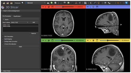
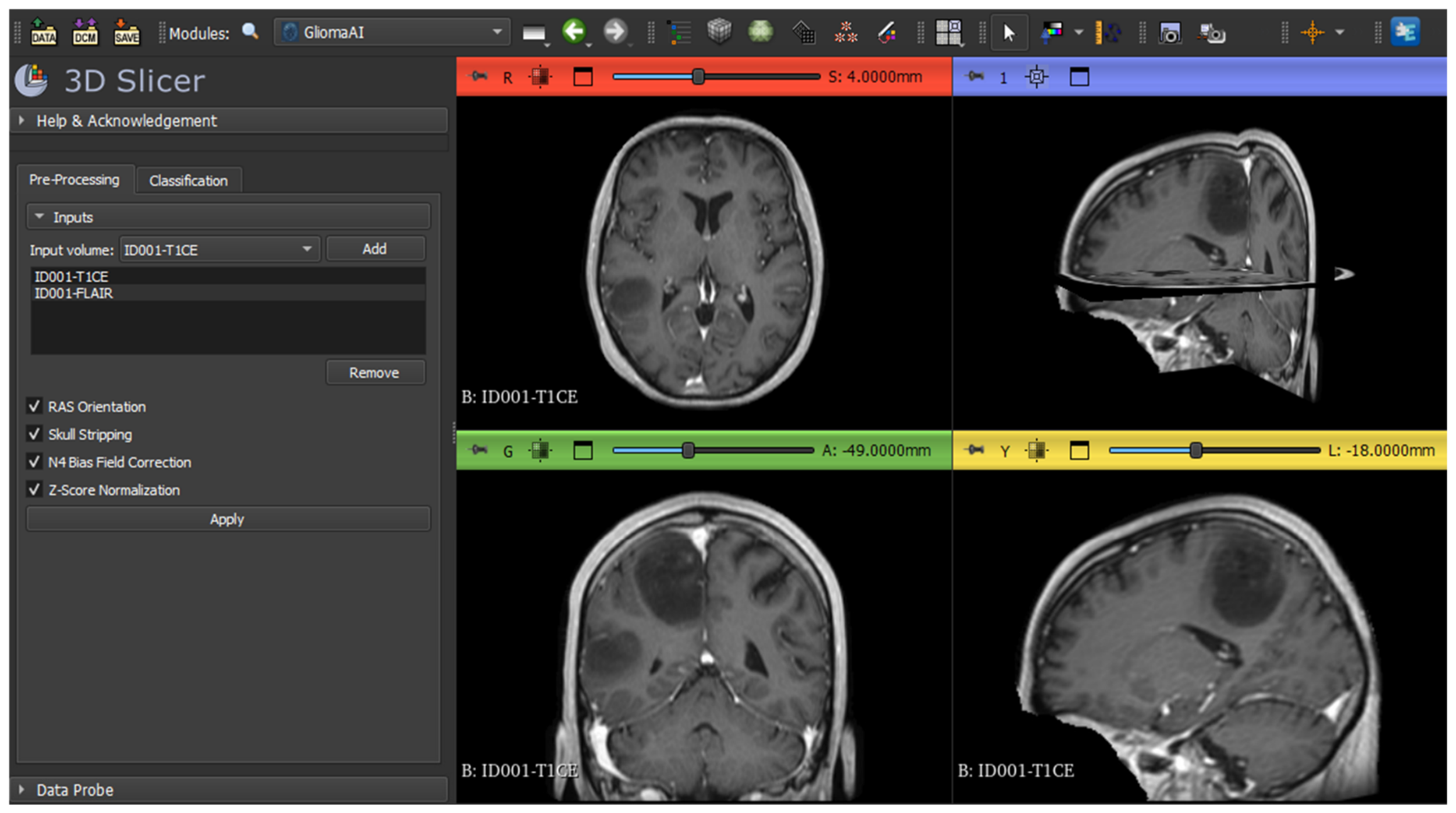
The preprocessing workflow incorporated into GliomaAI was adapted from our previous study [11]. Figure 2 illustrates the interface prior to preprocessing, where users can add one to four MRI volumes loaded into 3D Slicer to the processing list, remove selected entries, and configure the available operations through checkboxes. All configurable operations are enabled by default and constitute the recommended configuration. However, users can deselect individual steps when equivalent preprocessing has already been performed on the input volumes.
Figure 2.
Overview of the GliomaAI preprocessing tab within the 3D Slicer environment. The interface shows representative input volumes added to the preprocessing list and the available options before their application. One of the unprocessed MRI volumes is displayed in the standard anatomical views.
Processing is initiated by the Apply button, after which each listed MRI volume is processed sequentially. Each volume is first resampled to 1 mm3 voxel spacing through cubic spline interpolation. This mandatory operation establishes a consistent spatial resolution for subsequent processing and downstream use. The enabled operations are then applied, comprising RAS orientation, automated skull-stripping using SynthStrip [27], N4 bias field correction [32], and brain-masked z-score normalization. Cropping and padding are excluded at this stage because they constitute model-specific spatial standardization performed during input preparation for CNN classification. Keeping these operations separate preserves the standalone functionality of the preprocessing tool for external workflows.
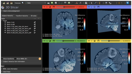
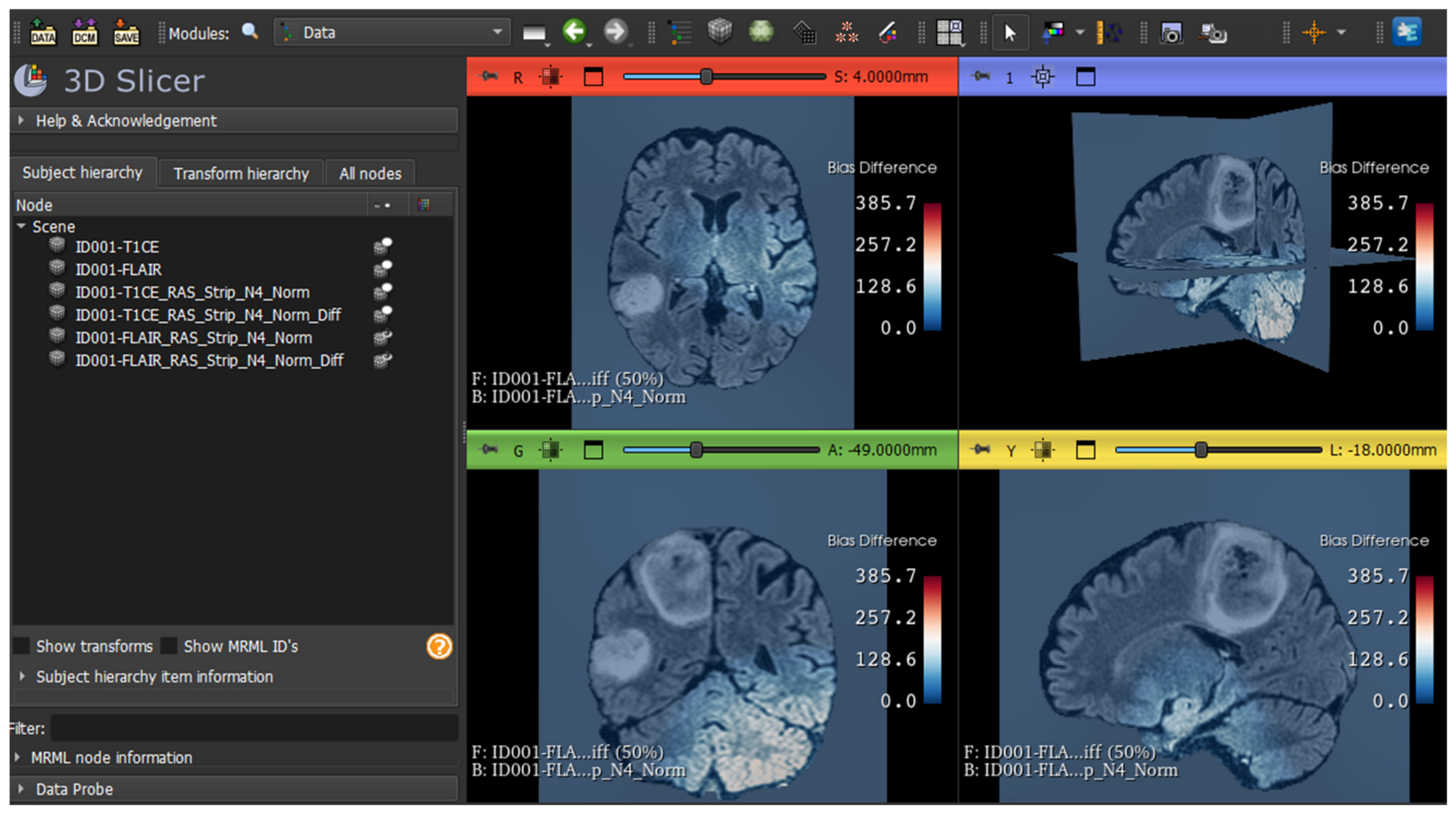
Upon completion, GliomaAI adds the processed outputs to the MRML scene as new volume nodes while preserving the original input volumes. Users can subsequently export these volumes in any format supported by 3D Slicer. When N4 bias field correction is enabled, an additional difference map is generated to visualize the intensity changes introduced by the correction. This map is displayed as an overlay with 50% opacity on the processed volume, together with the corresponding color bar indicating the magnitude of intensity differences, thereby providing a quality-control mechanism for inspecting the spatial effect of bias field correction. Figure 3 illustrates the preprocessing results for the representative input volumes and the corresponding output nodes displayed in the 3D Slicer Data module. Each processed volume retains the name of its original input supplemented with suffixes identifying the preprocessing operations applied.
Figure 3.
Overview of the preprocessing outputs generated by GliomaAI within the 3D Slicer environment. The Data module shows the original input volumes and the corresponding processed volume nodes. The last representative processed volume is displayed in the standard anatomical views with the N4 difference heatmap overlaid and accompanied by the corresponding color bar.
2.4. Classification and Explainability Workflow
Classification constitutes the principal analytical function of GliomaAI. Convolutional Neural Networks (CNNs) learn hierarchical image representations through successive layers of trainable convolutional filters, transforming low-level spatial patterns into high-level feature embeddings that support the estimation of class probabilities [33]. When trained on representative imaging cohorts, these models can capture task-relevant patterns and contribute to the detection, characterization, and monitoring of oncological abnormalities, thereby supporting clinical decision-making process [34].
The classification component of GliomaAI integrates our previously developed 3D CNN [11], referred to in the present work as GliomaAI-CNN, together with the established ResNet-10 [35], ResNet-50 [35], and DenseNet-121 [36] architectures. Following their evaluation through repeated five-fold cross-validation in the previous study, final deployment versions of the four networks were trained from scratch for a maximum of 50 epochs on the complete multicenter dataset of 1194 patients (442 LGG and 752 HGG), comprising 2213 MRI volumes from T1-CE and FLAIR sequences. Cases with a missing sequence were retained and the absent input channel was zero-filled. No explicit channel dropout was applied. Training was performed using the available HPC resources, a single NVIDIA A100 GPU with 40 GB VRAM.
The training protocol included a batch size of 5, the Adam optimizer with a learning rate of 1 × 10⁻⁴ and the sparse categorical cross-entropy loss function, consistent with the configurations used in the previous study’s cross-validation scheme. Early stopping was applied with a patience of 7 epochs based on training loss, with the weights corresponding to the lowest training loss restored at the end of training. The preprocessing, architectural, and optimization configurations established during model evaluation remained unchanged. To limit the extension package size, the resulting model weights are either already included or automatically retrieved upon first use and subsequently loaded for CPU-based inference.
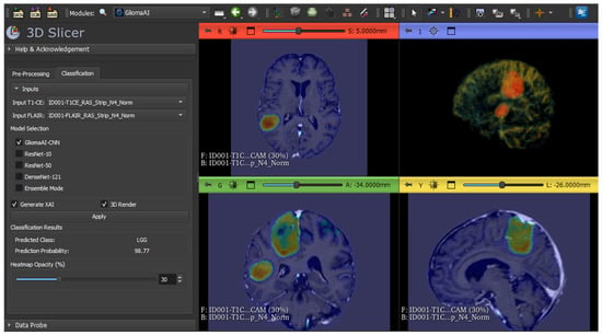
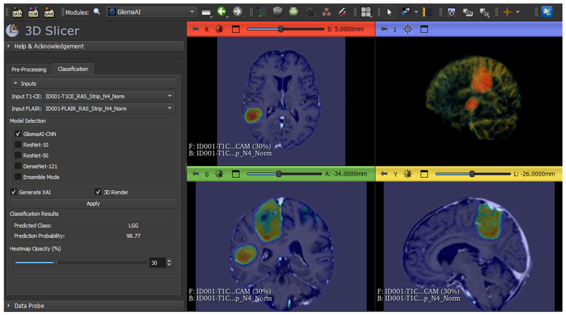
The user interaction and principal outputs of the classification and explainability workflow are illustrated in Figure 4, which presents the classification tab of the GUI, together with the classification results and explainability visualizations generated from a representative pair of volumes. For classification, users select the preprocessed T1-CE and FLAIR volumes from the MRML scene through the corresponding input selectors. Although both modalities constitute the recommended input configuration, classification can also be performed when only one of them is available. This functionality follows the missing modality strategy used during the training of the networks [11], whereby the input channel corresponding to the unavailable sequence undergoes zero-filling. Single-sequence performance was not evaluated in the present study, as both sequences were available for all cases. Before inference, the selected volumes undergo final spatial standardization, during which each volume is symmetrically padded or center-cropped along each axis to obtain fixed dimensions of 240 × 240 × 180 voxels (x, y, z). These operations are performed at the classification stage because the integrated CNNs require consistently sized input arrays for inference.
Figure 4.
Overview of the GliomaAI classification and explainability workflow within the 3D Slicer environment. The interface shows representative T1-CE and FLAIR volumes selected for classification, with the predicted LGG/HGG class and probability displayed in the classification tab. Explainability results are shown as Grad-CAM overlays in the anatomical planes and a 3D rendering.
After specifying the input volumes, users can select one of the four integrated CNNs for individual inference or combine multiple networks through the ensemble mode. For individual inference, the class probabilities are obtained directly from the selected network. In ensemble mode, the class probabilities generated by the participating networks are averaged with equal weights, enabling different combinations of the available models to contribute to the final prediction. In both cases, the class with the highest probability is returned as the final LGG/HGG prediction, corresponding to a fixed threshold of 0.50 for the HGG class. This decision rule is applied uniformly across all classification configurations, without threshold calibration or optimization using the external evaluation cohort. The predicted class and corresponding probability are then displayed in the GUI, as shown in Figure 4.
Classification is followed by the explainability analysis upon user selection of the Generate XAI checkbox. Gradient-weighted Class Activation Mapping (Grad-CAM) was employed as the interpretation technique. Grad-CAM utilizes class-specific gradients backpropagated to the feature maps of a target convolutional layer (typically the final convolutional layer) to generate heatmaps highlighting the most salient image regions that contributed positively to the resulting prediction [37]. In the present study, the progressive reduction in spatial resolution across successive network stages posed a challenge for Grad-CAM, particularly in architectures involving extensive spatial downsampling, such as DenseNet-121. Therefore, target layer selection required balancing the class-discriminative features provided by deeper layers with sufficient spatial resolution to limit localization loss when resampling the heatmaps to the input volume. Accordingly, architecture-specific target layers were predefined following qualitative examination of the generated heatmaps. The specific target layer selected for each architecture is detailed in Table A1.
The resulting heatmap is resampled to match the spatial dimensions of the input volume using trilinear interpolation, added to the MRML scene as a volume node, and automatically displayed as an overlay on the anatomical image. Following complete spatial restoration, possible negative values are removed, and the heatmap is normalized to the 0–1 range based on its maximum value. Grad-CAM maps are generated with respect to the predicted class. Grad-CAM generation is available only for individual CNN inference, as in ensemble mode the combination of multiple attribution maps could produce an ambiguous composite heatmap. Users can inspect the highlighted regions across axial, sagittal, and coronal planes of 3D Slicer GUI, by navigating through slice positions. The overlay is displayed with a default opacity of 70%, which can be interactively adjusted from 0% (fully transparent) to 100% (fully opaque) through the corresponding slider, as shown in Figure 4.
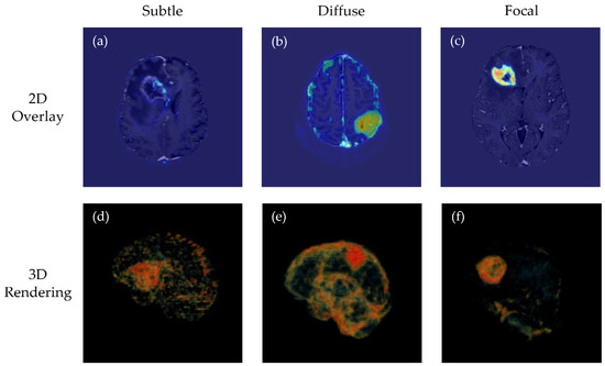
In addition to 2D overlay, GliomaAI provides an optional 3D rendering via the corresponding check box, allowing users to inspect the spatial distribution of Grad-CAM responses in greater detail within the same workflow. Direct, unadjusted rendering of the raw heatmap or the application of a fixed threshold was considered unsuitable because activations varied across cases, producing heterogeneous patterns ranging from subtle or diffuse to focal-strong patterns. Therefore, to ensure robust visualization across these diverse distributions, a multi-percentile rendering scheme was implemented. Figure 5 illustrates three representative cases, presenting an axial raw Grad-CAM overlay and the corresponding 3D rendering visualization for subtle, diffuse, and focal activation patterns.
Figure 5.
Representative 2D Grad-CAM overlays (a–c) and corresponding adaptive 3D renderings (d–f), generated from the GliomaAI-CNN heatmaps using the same percentile-based rendering procedure. The cases illustrate a subtle, low-contrast response (a,d), a diffuse activation distribution (b,e), and a strong focal activation (c,f).
In a related study, the percentile thresholds maximizing overlap between saliency maps and annotated tumor regions vary substantially across cases, with optimal values ranging from the 71st to the 96th percentile in the evaluated samples [38]. These findings motivated the use of multiple activation levels for visualization in the present study. Following near-background exclusion, the distribution of the remaining active voxels determines five percentile-based control points for the continuous opacity and RGB color transfer functions. The 55th and 75th percentiles define the onset of visibility and low-opacity spatial context, respectively. The 92nd percentile marks the principal transition, while the 98th and 99.7th percentiles represent the high and peak responses, which receive greater opacity and warmer colors. These rendering parameters were determined empirically through iterative qualitative evaluation of representative GliomaAI-CNN heatmaps, selected due to their comparatively high spatial detail. The same adaptive procedure is automatically applied to each case, eliminating the need for manual adjustment by the user.
2.5. External Evaluation Using the GliomaAI Extension
Following completion of the extension development, an independent patient-level evaluation was conducted by processing the external cases through the GliomaAI workflow. The evaluation assessed both the classification performance of the integrated models and their corresponding classification inference times. The publicly available training cohort of the 2019 Brain Tumor Segmentation Challenge (BraTS-19) was utilized for the assessment. It comprised 335 preoperative glioma patients, including 76 LGG and 259 HGG cases, with four MRI sequences available per patient [39,40,41]. Of these, the corresponding T1-CE and FLAIR volumes were used as inputs to the GliomaAI workflow.
To ensure patient-level independence and prevent data leakage between BraTS-19 cohort and the multicenter dataset of 1194 patients previously used for model development, a two-stage eligibility assessment process was performed. First, an overlap check was performed to ensure that no individual patient was represented in both datasets, irrespective of the number or type of MRI volumes available for that patient. Because the BraTS-19 cohort includes cases originating from TCGA-LGG, the official BraTS 2017–2023_GLI patient mapping file, provided by the respective data holders, was used together with the official TCGA-LGG mapping file to identify the corresponding original TCGA-LGG patient identifiers for BraTS-19 cases. These original patient identifiers were then compared with those of the 1194-patient model-development cohort, and all overlapping patients were excluded.
As the second stage, the remaining non-overlapping cases underwent image quality assessment. The T1-CE and FLAIR volumes of each case were visually inspected by the study authors in 3D Slicer before entering GliomaAI workflow. Cases were retained or excluded based on unanimous agreement among three independent observers, and no disagreements occurred. The assessment was performed prior to any model evaluation, using predefined technical criteria, and was based solely on the technical characteristics of the MRI volumes, regardless of tumor grade. Cases presenting severe artifacts were excluded. These included incomplete anatomical coverage due to cropping of brain tissue (normal or tumoral), which limited the anatomical information and could compromise the reliability of the workflow’s output, as well as pronounced noise and signal degradation, such as excessive blurring attributable to motion or other artifacts of unknown origin. Cases with only minimal cropping were retained. The final cohort comprised 234 cases, including 26 LGG and 208 HGG cases. Table 2 reports the number of cases excluded at each stage and the corresponding number retained by class.
Table 2.
Patient-level eligibility assessment of the BraTS-19 external cohort, reporting excluded cases and final composition by glioma grade.
As the BraTS-19 images were already provided in post skull-stripping form, the corresponding preprocessing step was disabled to avoid redundant processing. Notably, 39.4% of the development cohort had likewise been provided in skull-stripped form, so the models had already been exposed to heterogeneity in skull-stripping procedures, potentially mitigating the introduction of preprocessing-related domain shift. All remaining operations were applied as described in Section 2.3. Each integrated CNN and the ensemble configuration were evaluated across all cases in the final cohort, with HGG designated as the positive class.
Given the marked imbalance between the two glioma categories, the numbers and proportions of correctly classified cases are reported separately. The corresponding 95% confidence intervals (CIs) for sensitivity and specificity were calculated using the Wilson score method without continuity correction [42]. Discriminative performance was additionally assessed using balanced accuracy, defined as the mean of HGG sensitivity and LGG specificity [43], with its 95% CI estimated using stratified bootstrap resampling with 10,000 repetitions [44]. The Matthews Correlation Coefficient (MCC), Positive Predictive Value (PPV), and Negative Predictive Value (NPV) were also calculated. Finally, performance across classification thresholds was assessed using the area under the receiver operating characteristic curve (ROC-AUC), with its 95% CI estimated using the DeLong method [45]. Differences in ROC-AUC between configurations were assessed using the paired DeLong test, as all models were evaluated on the same cases, and p-values were adjusted for the ten pairwise comparisons using the Holm method (adjusted p < 0.05 was considered statistically significant).
To quantitatively assess the faithfulness of the XAI explanations generated using Grad-CAM, a perturbation-based deletion analysis was performed, measuring the decrease in the predicted class probability after removing the voxels ranked as most relevant, relative to the removal of an equal number of randomly selected voxels [46,47]. The analysis was implemented in the Python console of 3D Slicer for the four individual networks, using the same preprocessing and inference pipeline as the classification experiments, with the preprocessed volumes computed once and reused across all models. For each case, the predicted class and its probability were obtained from the intact volumes, and a Grad-CAM heatmap for the predicted class was generated. Non-background voxels were ranked by heatmap value, and the top 5%, 10%, 20% and 30% were set to zero in both modalities, after which the drop in the predicted-class probability relative to the intact volumes was recorded. The same procedure was repeated with an equal number of randomly selected non-background voxels, and the drop was averaged over three repetitions per fraction.
3. Results
3.1. Technical Implementation and Computational Performance
The GliomaAI extension was successfully completed, resulting in a functional tool integrated within 3D Slicer environment. Its functionality was confirmed through the successful execution of the implemented workflow, including volume preprocessing, inference with each individual CNN and the ensemble configuration, and Grad-CAM visualization. All 468 T1-CE and FLAIR volumes included in the external evaluation underwent preprocessing with no execution failures observed and classification outputs were generated for all 234 patient cases using each inference configuration. The resulting classification performance is reported separately in Section 3.2.
Following functional verification, the technical runtime performance of the integrated models was assessed using the mentioned CPU resources. The recorded classification execution time covered model selection and availability checks, model loading and inference, probability processing, and display of the final prediction in the GUI. Measurements were collected for each individual CNN and the ensemble configuration for all cases included in the external evaluation. Before data collection, all required dependencies had been installed, retrieval of the network weights had been completed, and each network had already been invoked to complete its initial loading and framework initialization.
Table 3 summarizes the mean classification times for subsequent executions with the corresponding sample standard deviations in seconds, providing an indicative estimate of execution time and a comparison across configurations under the same measurement conditions. Mean times ranged from 0.27 to 1.53 s for individual CNNs, while the ensemble mode, which included inference with all integrated networks, required a mean time of 3.18 s.
Table 3.
Classification execution time for each configuration of the GliomaAI. Results are reported as mean ± standard deviation in seconds.
3.2. External Evaluation of Classification Performance
In this section, the results of the external evaluation conducted on the BraTS-19 cohort using the GliomaAI module are presented. All input volumes underwent the required preprocessing steps, after which inference was performed separately using each integrated CNN and the ensemble mode. Table 4 reports the number and proportion of the correctly classified LGG cases (the negative class, as HGG was designated as the positive class) for each evaluated configuration. Performance is expressed as specificity accompanied by the corresponding Wilson score 95%CIs. ResNet-10 achieved the highest performance, correctly classifying all examined cases. Nevertheless, despite the observed specificity of 100%, confidence remained relatively wide (87.1–100.0) because of the small LGG sample size.
Table 4.
Classification performance for LGG cases in the external BraTS-19 cohort, reported as correctly classified cases (n/N) and specificity with 95% CIs.
Additionally, Table 5 presents the classification results for HGG cases (the positive class) across all configurations within the GliomaAI extension. GliomaAI-CNN achieved the highest performance, with a sensitivity of 95.2%, clearly outperforming the other models. Regarding confidence, the larger number of HGG cases resulted in narrower 95% CIs, providing more reliable estimation of performance.
Table 5.
Classification performance for HGG cases in the external BraTS-19 cohort, reported as correctly classified cases (n/N) sensitivity with 95% CIs.
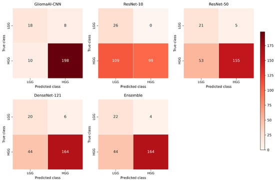
Figure 6 provides a visual summary of the classification outcomes for all configurations on the external BraTS-19 cohort. In each confusion matrix, rows correspond to the true class and columns to the predicted class, with HGG designated as the positive class and LGG as the negative class. The diagonal cells represent correctly classified cases.
Figure 6.
Confusion matrices of all evaluated configurations on the external BraTS-19 cohort.
An overview of the performance of all evaluated configurations is provided in Table 6. GliomaAI-CNN achieved the highest performance with balanced accuracy of 82.2% and MCC of 62.4%. PPV and NPV were 96.1% and 64.3%, respectively, whereas ResNet-10 achieved a PPV of 100% but a substantially lower NPV of 19.3%. The ensemble mode exhibited the second-best overall performance.
Table 6.
Overall classification performance for all configuration evaluated in the external BraTS-19 cohort, including balanced accuracy with bootstrap derived 95% CIs, MCC, PPV, and NPV.
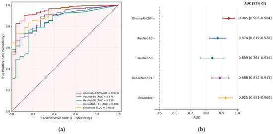
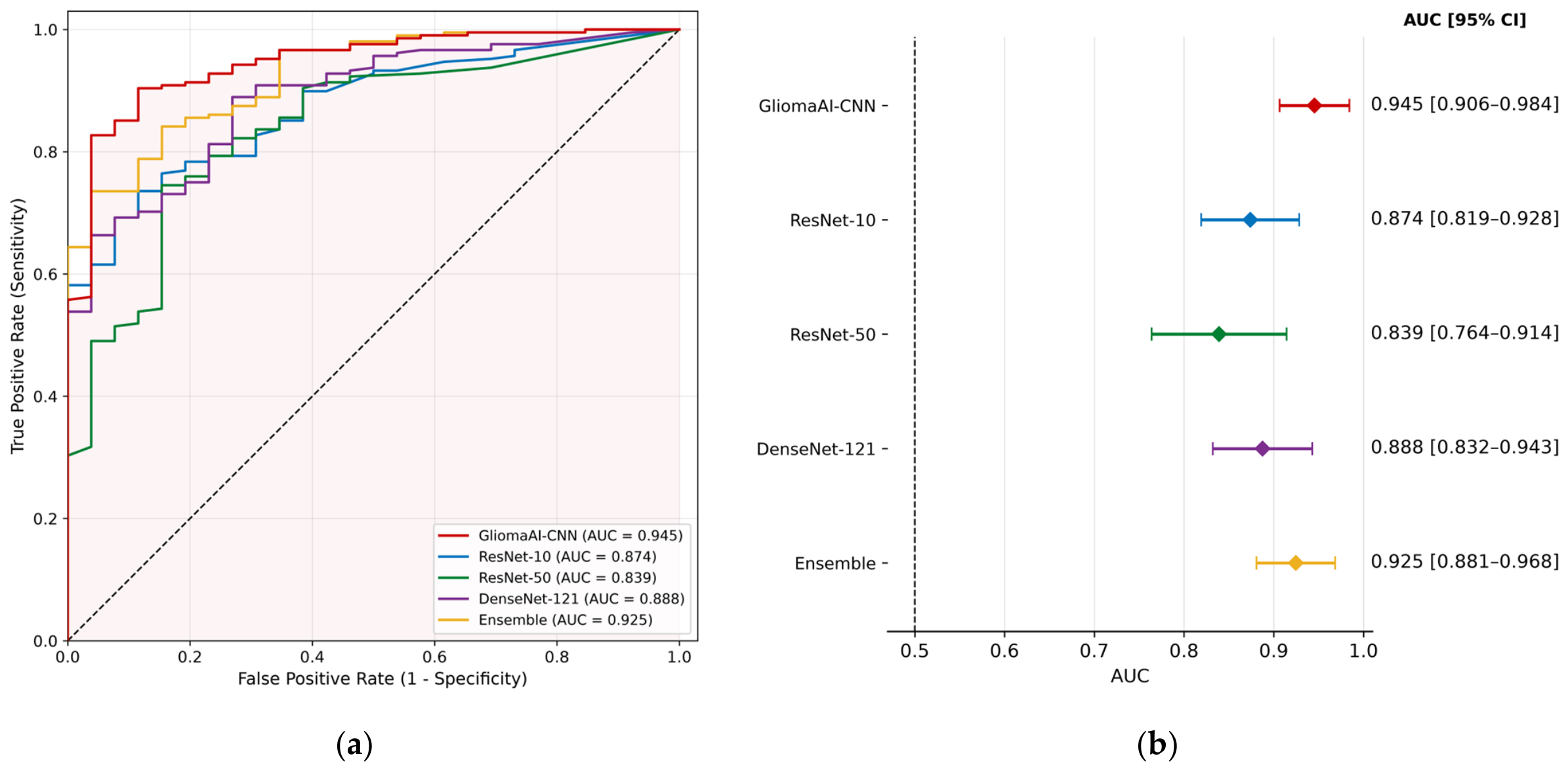
A more detailed perspective on the external evaluation of BraTS-19 cases is provided in Figure 7 which considers the probability outputs generated by GliomaAI. Figure 7a presents the ROC and the corresponding AUC values, while the forest plot in Figure 7b displays the AUC estimates with their corresponding DeLong 95% CIs. Among the evaluated configurations, GliomaAI-CNN achieved the highest AUC point estimate of 0.945, followed by the ensemble configuration with an AUC of 0.925. These two configurations also exhibited the narrowest CIs among the evaluated models. Paired DeLong comparisons with Holm correction (Table A2) further showed that both configurations achieved a statistically significant higher AUC than ResNet-50 (adjusted p = 0.014 and 0.007, respectively), with no significant difference detected between them. The lower bounds of all CIs were above 0.50.
Figure 7.
Comparison of the discrimination performance of each inference configuration during external evaluation on the BraTS-19 cohort using the GliomaAI extension: (a) receiver operating characteristic (ROC) curves with the corresponding area under the curve (AUC) values; (b) forest plot of the AUC with the corresponding DeLong 95% CIs. The diagonal dashed line in (a) represents the reference performance of a random classifier.
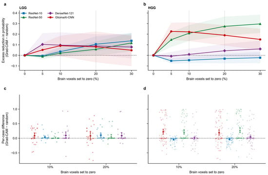
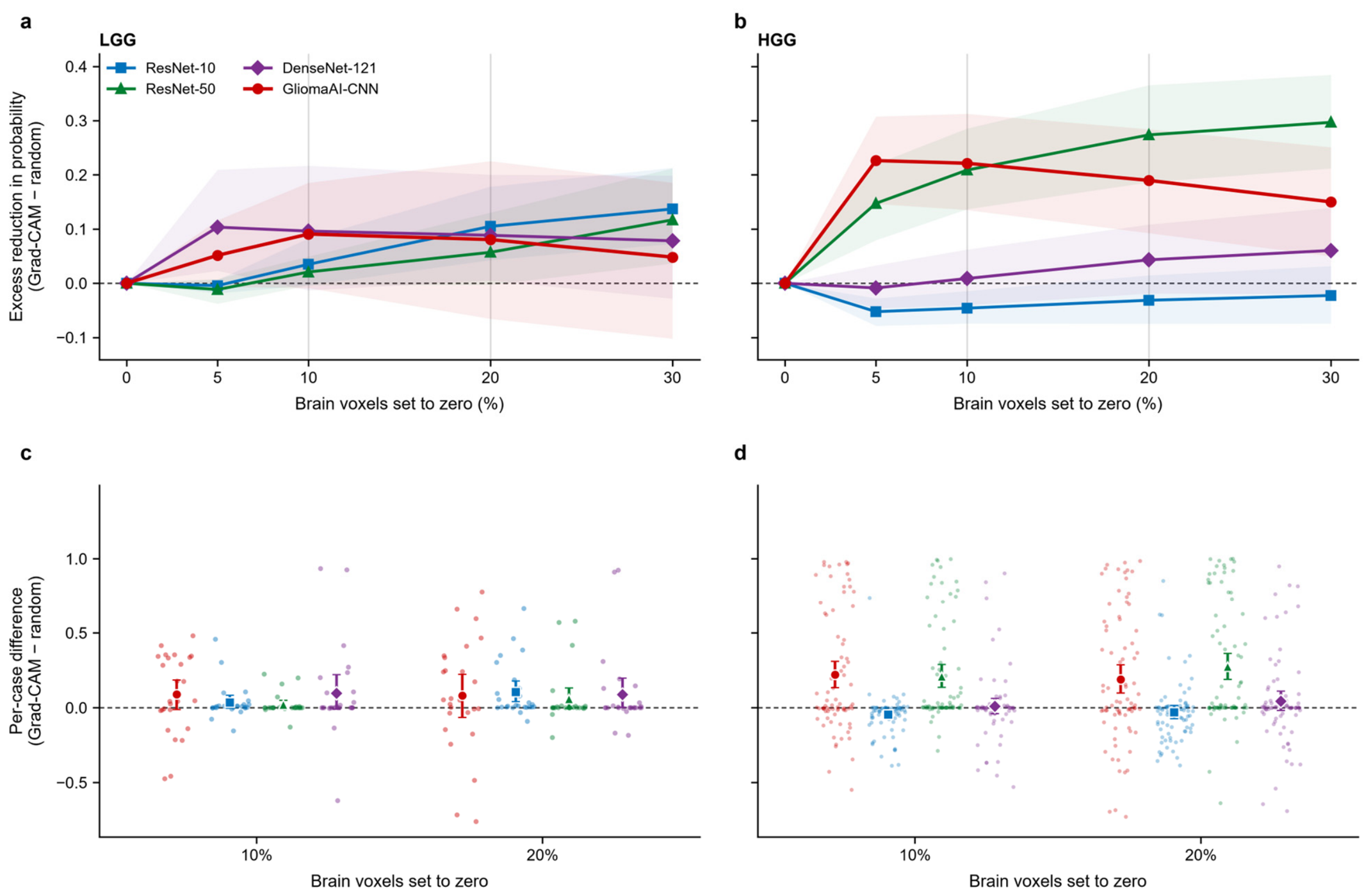
The quantitative faithfulness evaluation of the 3D Grad-CAM explanations on the external validation cohort is presented in Figure 8. Specifically, Figure 8a,b present the mean excess reduction in predicted class probability across progressive voxel removal fractions (5–30%), while Figure 8c,d illustrate the corresponding per-case difference distributions at the predefined 10% and 20% thresholds. Positive values indicate that removing the voxels ranked as most relevant by Grad-CAM reduced the predicted-class probability more than removing an equal number of random voxels, whereas values near zero or negative indicate no advantage over random removal.
Figure 8.
Quantitative faithfulness of 3D Grad-CAM explanations on the external validation cohort across the four deployed architectures. (a,b) Mean excess reduction in the predicted class probability (Grad-CAM-guided minus random removal) as a function of the percentage of brain voxels set to zero, for LGG and HGG cases respectively. (c,d) Per-case differences (Grad-CAM minus random) at 10% and 20% voxel removal thresholds for LGG and HGG cases respectively. Each dot represents an individual patient case, and markers with error bars indicate the mean with 95% bootstrap CIs.
In the LGG subgroup, all four architectures exhibited a positive mean excess reduction in predicted class probability as larger fractions of salient brain voxels were masked, although the 95% bootstrap confidence intervals remained relatively wide due to the smaller sample size. In HGG cases, the differences between architectures were more pronounced. GliomaAI-CNN showed the largest excess reduction at the smallest fractions (5–10%) and then declined gradually with further removal. ResNet-50 approached GliomaAI-CNN at 10% removal and exceeded it at 20% and 30%, with Figure 8d confirming that the 95% confidence intervals of both models remained clearly above zero at the 10% and 20% thresholds. Conversely, DenseNet-121 showed only marginal positive values, while ResNet-10 remained slightly below zero across all removal fractions.
4. Discussion
AI models have already achieved impressive performance across a wide range of medical diagnostic tasks, highlighting their potential to contribute positively to various clinical workflows. When incorporated into decision support applications, these models can leverage knowledge derived from previously collected datasets to provide patient-specific assessments that support clinical decision-making. Their purpose, however, is to augment rather than replace clinical expertise, with clinicians retaining responsibility for the final evaluation and judgement. Such systems must meet important requirements, including explainability, reliability and usability [48,49]. Nevertheless, translating AI models into medical imaging applications and subsequently integrating them into clinical practice remains challenging. In this context, integrated and interpretable software tools represent an important intermediate step bridging algorithmic research and practical clinical deployment.
GliomaAI addresses this translational need by providing two complementary functional frameworks through the 3D Slicer platform within a unified and accessible environment. First, the integration of preprocessing workflow enables a standardized preparation of MRI volumes for subsequent LGG/HGG classification, while retaining functionality for external image analysis tasks. Second, the classification workflow incorporates previously evaluated CNN architectures, with their final deployment versions retrained on a large multi-cohort dataset of 1194 patients, and enables automated glioma grading from the preprocessed volumes. Its segmentation-free design removes the requirement for expert tumor delineation or a preceding automated segmentation, both of which are time-consuming and may introduce errors that can affect the subsequent classification process. This simplifies the overall workflow by eliminating the need for a separate segmentation model and reduces the number of processing steps required for classification. Classification was also computationally efficient after model initialization, with subsequent inference times ranging from 0.27 to 1.53 s for the individual networks and reaching 3.18 s for the ensemble configuration. Collectively, these characteristics support the accessibility and technical feasibility of the proposed workflow for glioma image assessment.
Furthermore, the integration of Explainable Artificial Intelligence (XAI) through Grad-CAM into the GliomaAI classification workflow extends the model output, providing an important step into analysis. Given the “black-box” nature of deep neural networks, the ability to inspect the image regions associated with a prediction is particularly relevant to their potential use in clinical decision support. The EU AI Act also established a regulatory framework requiring transparency to support the interpretation of outputs from high-risk AI systems [50]. The generated heatmaps can be interactively overlaid on either the T1-CE or FLAIR volume and examined in axial, sagittal, and coronal views. This enables the activation patterns to be interpreted alongside the corresponding anatomical characteristics. Evaluation across these different modalities can enhance clinician’s trust including the observation of activated contrast-enhancing tumor regions on T1-CE and edema-related abnormalities on FLAIR. Complementing the multiplanar 2D overlays, 3D rendering provides a global representation of the spatial distribution and extent of the displayed positive activations throughout the imaging volume. Inspection of significant more positively contributed areas in spatial view can provide a better estimation of system operation.
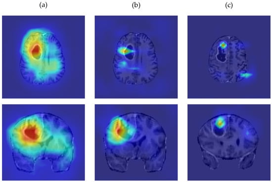
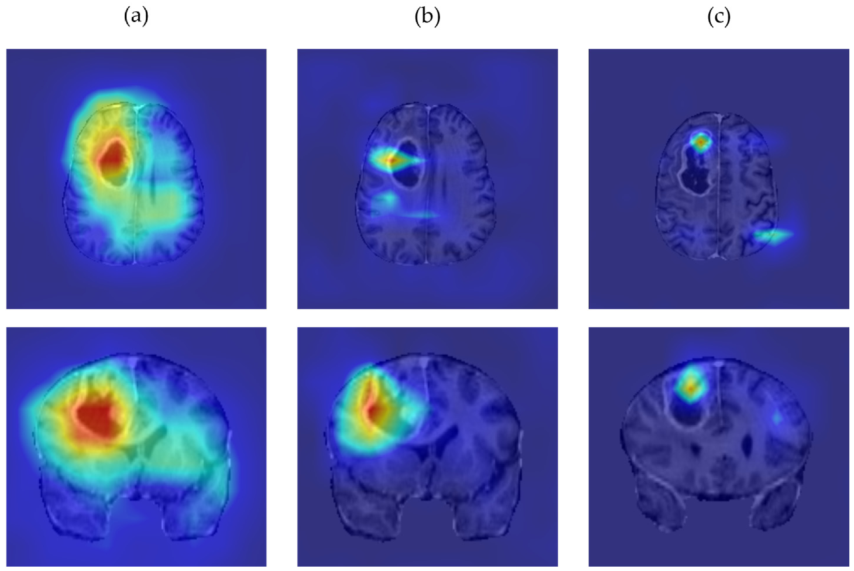
Nevertheless, the generated explainability visualizations present limitations that should be considered during their interpretation. Regarding 2D views, the deeper integrated classification architectures exhibited minor spatial deviations between their activation patterns and the visually apparent tumor regions, despite the applied layer-selection and visualization settings. Although the overall activation patterns remained anatomically plausible, their precise localization was limited by the low spatial resolution of the underlying convolutional feature maps. Figure 9 presents the axial and coronal heatmap overlays generated by ResNet-10, ResNet-50, and DenseNet-121 for a representative case, providing a qualitative illustration of these observations.
Figure 9.
Representative Grad-CAM heatmap overlays in axial and coronal views for (a) ResNet-10, (b) ResNet-50, and (c) DenseNet-121 networks. The activation patterns show minor spatial deviations from the visually apparent tumor region, which reflects the limited resolution of convolutional feature maps.
3D rendering also requires cautious interpretation because its visual appearance is influenced by heatmap thresholding and opacity settings. Despite the broad range of activations that can be visualized through this approach, relatively low-intensity activations may form a visually prominent volume after rendering, potentially overemphasizing their apparent relevance to the model’s prediction. Specifically, the 55th percentile, which sets the lower bound of visibility, represents a relative rather than an absolute activation threshold and does not discriminate tumor from normal tissue activation, as Grad-CAM does not constitute a segmentation method. Activations appearing outside the main tumor region at lower percentile settings should not be interpreted as evidence of additional tumor involvement. The 3D representation should therefore be regarded as complementary and evaluated by specialists alongside the corresponding anatomical images and 2D heatmap overlays.
Regarding external validation on the non-overlapping BraTS-19 cohort, GliomaAI-CNN achieved the highest observed balanced accuracy (82.2%), MCC (62.4%), and AUC (0.945) among the evaluated configurations, suggesting that the task-specific architecture identified through neural architecture search (NAS) retained its discriminative ability outside the model-development cohort. Specifically, this architecture showed the highest sensitivity for HGG (95.2%) but the lowest specificity (69.2%). Conversely, ResNet-10 identified all LGG cases (specificity of 100%) but had the lowest sensitivity. The equal-weight ensemble achieved the second-best performance but did not surpass GliomaAI-CNN alone, possibly because of the inclusion of lower-performing constituent networks. The specificity estimates should be interpreted with particular caution, as they were based on only 26 cases compared with 208 HGG cases, which is reflected in their wider confidence intervals. Notably, with only 26 LGG cases, each misclassification alters specificity by approximately 3.85 percentage points, which increases statistical uncertainty. For a potential clinical decision support application, sensitivity to HGG warrants attention because classifying an HGG as LGG could underestimate tumor severity [51].
Beyond discriminative performance, the quantitative faithfulness analysis showed that the reliability of the Grad-CAM explanations was architecture-dependent. In HGG cases, GliomaAI-CNN and ResNet-50 showed a consistent advantage of Grad-CAM-guided over random voxel removal, whereas DenseNet-121 and ResNet-10 showed little or no advantage, indicating that Grad-CAM heatmaps should not be assumed to be equally reliable across architectures. Notably, GliomaAI-CNN showed its largest excess reduction when only the top 5–10% of ranked voxels were removed, a small fraction of the brain volume comparable to a tumor’s extent, suggesting that the heatmaps identified early a compact region driving the prediction, plausibly the tumor. In LGG cases, the effect was modest and uncertain, likely reflecting the small sample size. Overall, such systems may provide useful non-invasive preoperative estimates, but their outputs should support specialist assessment rather than be treated as definitive diagnoses.
A post-hoc exploratory analysis was conducted to compare the default threshold (0.50) results with an optimized one, as presented in Table A3. Specifically, the threshold maximizing Youden’s J (sensitivity + specificity − 1) was identified for each configuration [52]. Although the resulting thresholds increased balanced accuracy across all configurations, MCC did not improve uniformly. This lack of uniformity may partly reflect a class-prevalence (prior) shift between the development cohort (63% HGG) and the external cohort (89% HGG), to which MCC is sensitive and which can make the default threshold suboptimal. These findings should be interpreted cautiously because the thresholds were selected using the same cohort on which performance was assessed.
The present evaluation relied on a retrospectively assembled dataset and did not assess the extension in prospective clinical use. Together with the small number of LGG cases and the class imbalance, this limits the generalizability of the findings to other scanners, acquisition protocols, and patient populations. Accordingly, GliomaAI should currently be regarded as a research tool, and the present evidence does not support its clinical deployment. Further validation on an independent cohort of locally acquired MRI examinations, ideally with a more balanced distribution of LGG and HGG cases, is needed to robustly examine its performance under routine conditions. Direct clinician feedback is also warranted to evaluate the usability and compatibility of the complete workflow, as well as how its predictions and visual explanations are interpreted in practice. Additionally, functional testing was performed only on Windows 11, while compatibility and runtime behavior on Linux and macOS remain to be verified. Weighted or selective ensemble strategies were also not evaluated and could be explored in future work. Beyond LGG/HGG classification, future directions could involve the integration of MRI-based predictions of critical molecular markers, such as IDH mutation status and 1p/19q codeletion, thereby supporting personalized patient assessment.
5. Conclusions
In conclusion, GliomaAI is an open-source 3D Slicer extension that integrates MRI preprocessing, segmentation-free LGG/HGG classification, and explainability. Unlike the comparable classification tools discussed in the Introduction, GliomaAI integrates previously evaluated CNN architectures with explainability through interactive Grad-CAM overlays and 3D heatmap rendering, allowing users to inspect regions associated with model predictions. External evaluation on a non-overlapping BraTS-19 cohort provided encouraging evidence of classification performance. This transparency may help clinicians assess the plausibility of model outputs and supports further investigation of GliomaAI as a clinical decision-support tool.
Author Contributions
Conceptualization, E.I.A. and C.C.A.; methodology, E.I.A. and C.C.A.; software, C.C.A.; writing—original draft preparation, C.C.A., S.A.K., I.K.K., D.T.G., P.A.A., D.A.C. and E.I.A.; supervision, E.I.A.; All authors have read and agreed to the published version of the manuscript.
Funding
This research received no external funding.
Institutional Review Board Statement
Not applicable.
Informed Consent Statement
Not applicable.
Data Availability Statement
This study analyzed data from the BraTS-19 dataset, described in [39,40,41]. The original MRI data are available through the dataset providers under their applicable access conditions. The source code of the GliomaAI extension is publicly available in the GitHub repository at https://github.com/xristosand/SlicerGliomaAI (accessed on 21 October 2026). The repository is under active maintenance and may receive technical updates after publication.
Conflicts of Interest
The authors declare no conflicts of interest.
Abbreviations
The following abbreviations are used in this manuscript:
| AI | Artificial Intelligence |
| AUC | Area Under the Curve |
| BraTS-19 | Brain Tumor Segmentation Challenge 2019 |
| CAD | Computer-Aided Diagnosis |
| CI | Confidence Interval |
| CNN | Convolutional Neural Network |
| CNS | Central Nervous System |
| FLAIR | Fluid-Attenuated Inversion Recovery |
| Grad-CAM | Gradient-Weighted Class Activation Mapping |
| GUI | Graphical User Interface |
| HGG | High-Grade Glioma |
| HPC | High-Performance Computing |
| LGG | Low-Grade Glioma |
| MCC | Matthews Correlation Coefficient |
| MRI | Magnetic Resonance Imaging |
| MRML | Medical Reality Modeling Language |
| NPV | Negative Predictive Value |
| PPV | Positive Predictive Value |
| ROC | Receiver Operating Characteristic |
| T1-CE | T1-Weighted Contrast-Enhanced |
| VTK | Visualization Toolkit |
| WHO | World Health Organization |
| XAI | Explainable Artificial Intelligence |
Appendix A
Table A1.
Overview of the convolutional layers selected as target layers for Grad-CAM heatmap generation in each integrated architecture of the GliomaAI extension.
Table A2.
Pairwise comparison of AUC values between model configurations on the BraTS-19 external cohort, using the paired DeLong test with Holm correction for multiple comparisons.
Table A3.
Post hoc exploratory analysis of the external BraTS-19 classification for all configurations of the GliomaAI extension, comparing the default decision threshold (0.50) with the Youden-optimal threshold (HGG = positive class; LGG = negative class).
References
- Luo, J.; Pan, M.; Mo, K.; Mao, Y.; Zou, D. Emerging Role of Artificial Intelligence in Diagnosis, Classification and Clinical Management of Glioma. Semin. Cancer Biol. 2023, 91, 110–123. [Google Scholar] [CrossRef] [Scilit] [PubMed]
- Weller, M.; Wen, P.Y.; Chang, S.M.; Dirven, L.; Lim, M.; Monje, M.; Reifenberger, G. Glioma. Nat. Rev. Dis. Primers 2024, 10, 33. [Google Scholar] [CrossRef] [Scilit] [PubMed]
- Louis, D.N.; Perry, A.; Wesseling, P.; Brat, D.J.; Cree, I.A.; Figarella-Branger, D.; Hawkins, C.; Ng, H.K.; Pfister, S.M.; Reifenberger, G.; et al. The 2021 WHO Classification of Tumors of the Central Nervous System: A Summary. Neuro-Oncol. 2021, 23, 1231–1251. [Google Scholar] [CrossRef] [Scilit] [PubMed]
- Zhuge, Y.; Ning, H.; Mathen, P.; Cheng, J.Y.; Krauze, A.V.; Camphausen, K.; Miller, R.W. Automated Glioma Grading on Conventional MRI Images Using Deep Convolutional Neural Networks. Med. Phys. 2020, 47, 3044–3053. [Google Scholar] [CrossRef] [Scilit] [PubMed]
- Bahar, R.C.; Merkaj, S.; Cassinelli Petersen, G.I.; Tillmanns, N.; Subramanian, H.; Brim, W.R.; Zeevi, T.; Staib, L.; Kazarian, E.; Lin, M.; et al. Machine Learning Models for Classifying High- and Low-Grade Gliomas: A Systematic Review and Quality of Reporting Analysis. Front. Oncol. 2022, 12, 856231. [Google Scholar] [CrossRef] [Scilit] [PubMed]
- Thust, S.C.; Heiland, S.; Falini, A.; Jäger, H.R.; Waldman, A.D.; Sundgren, P.C.; Godi, C.; Katsaros, V.K.; Ramos, A.; Bargallo, N.; et al. Glioma Imaging in Europe: A Survey of 220 Centres and Recommendations for Best Clinical Practice. Eur. Radiol. 2018, 28, 3306–3317. [Google Scholar] [CrossRef] [Scilit] [PubMed]
- Zhan, Y.; Hao, Y.; Wang, X.; Guo, D. Advances of Artificial Intelligence in Clinical Application and Scientific Research of Neuro-Oncology: Current Knowledge and Future Perspectives. Crit. Rev. Oncol. Hematol. 2025, 209, 104682. [Google Scholar] [CrossRef] [Scilit] [PubMed]
- Bhatele, K.R.; Bhadauria, S.S. Machine Learning Application in Glioma Classification: Review and Comparison Analysis. Arch. Comput. Methods Eng. 2022, 29, 247–274. [Google Scholar] [CrossRef] [Scilit]
- Chakrabarty, S.; Sotiras, A.; Milchenko, M.; LaMontagne, P.; Hileman, M.; Marcus, D. MRI-Based Identification and Classification of Major Intracranial Tumor Types by Using a 3D Convolutional Neural Network: A Retrospective Multi-Institutional Analysis. Radiol. Artif. Intell. 2021, 3, e200301. [Google Scholar] [CrossRef] [Scilit] [PubMed]
- Chen, Q.; Wang, L.; Deng, Z.; Wang, R.; Wang, L.; Jian, C.; Zhu, Y.-M. Cooperative Multi-Task Learning and Interpretable Image Biomarkers for Glioma Grading and Molecular Subtyping. Med. Image Anal. 2025, 101, 103435. [Google Scholar] [CrossRef] [Scilit] [PubMed]
- Andrianos, C.C.; Kostopoulos, S.A.; Kalatzis, I.K.; Glotsos, D.T.; Asvestas, P.A.; Cavouras, D.A.; Athanasiadis, E.I. Segmentation-Free Preoperative 3D MRI Classification of Low-Grade Versus High-Grade Glioma Using Task-Oriented Neural Architecture Search. J. Imaging 2026, 12, 254. [Google Scholar] [CrossRef] [Scilit] [PubMed]
- Abadi, M.; Barham, P.; Chen, J.; Chen, Z.; Davis, A.; Dean, J.; Devin, M.; Ghemawat, S.; Irving, G.; Isard, M.; et al. TensorFlow: A System for Large-Scale Machine Learning. arXiv 2016, arXiv:1605.08695. [Google Scholar]
- Paszke, A.; Gross, S.; Massa, F.; Lerer, A.; Bradbury, J.; Chanan, G.; Killeen, T.; Lin, Z.; Gimelshein, N.; Antiga, L.; et al. PyTorch: An Imperative Style, High-Performance Deep Learning Library. arXiv 2019, arXiv:1912.01703. [Google Scholar]
- Cardoso, M.J.; Li, W.; Brown, R.; Ma, N.; Kerfoot, E.; Wang, Y.; Murrey, B.; Myronenko, A.; Zhao, C.; Yang, D.; et al. MONAI: An Open-Source Framework for Deep Learning in Healthcare. arXiv 2022, arXiv:2211.02701. [Google Scholar]
- Gupta, V.; Erdal, B.; Ramirez, C.; Floca, R.; Genereaux, B.; Bryson, S.; Bridge, C.; Kleesiek, J.; Nensa, F.; Braren, R.; et al. Current State of Community-Driven Radiological AI Deployment in Medical Imaging. JMIR AI 2024, 3, e55833. [Google Scholar] [CrossRef] [Scilit] [PubMed]
- Tejani, A.S.; Cook, T.S.; Hussain, M.; Sippel Schmidt, T.; O’Donnell, K.P. Integrating and Adopting AI in the Radiology Workflow: A Primer for Standards and Integrating the Healthcare Enterprise (IHE) Profiles. Radiology 2024, 311, e232653. [Google Scholar] [CrossRef] [Scilit] [PubMed]
- Fedorov, A.; Beichel, R.; Kalpathy-Cramer, J.; Finet, J.; Fillion-Robin, J.-C.; Pujol, S.; Bauer, C.; Jennings, D.; Fennessy, F.; Sonka, M.; et al. 3D Slicer as an Image Computing Platform for the Quantitative Imaging Network. Magn. Reson. Imaging 2012, 30, 1323–1341. [Google Scholar] [CrossRef] [Scilit] [PubMed]
- Amla, Z.; Khehra, P.S.; Mathialagan, A.; Lugez, E. Review of the Free Research Software for Computer-Assisted Interventions. J. Imaging Inform. Med. 2024, 37, 386–401. [Google Scholar] [CrossRef] [Scilit] [PubMed]
- Pati, S.; Singh, A.; Rathore, S.; Gastounioti, A.; Bergman, M.; Ngo, P.; Ha, S.M.; Bounias, D.; Minock, J.; Murphy, G.; et al. The Cancer Imaging Phenomics Toolkit (CaPTk): Technical Overview. In Brainlesion: Glioma, Multiple Sclerosis, Stroke and Traumatic Brain Injuries; Crimi, A., Bakas, S., Eds.; Lecture Notes in Computer Science; Springer International Publishing: Cham, Switzerland, 2020; Volume 11993, pp. 380–394. [Google Scholar]
- Mehrtash, A.; Pesteie, M.; Hetherington, J.; Behringer, P.A.; Kapur, T.; Wells, W.M.; Rohling, R.; Fedorov, A.; Abolmaesumi, P. DeepInfer: Open-Source Deep Learning Deployment Toolkit for Image-Guided Therapy. Proc. SPIE Int. Soc. Opt. Eng. 2017, 10135, 101351K. [Google Scholar] [CrossRef] [Scilit] [PubMed]
- Zeineldin, R.A.; Weimann, P.; Karar, M.E.; Mathis-Ullrich, F.; Burgert, O. Slicer-DeepSeg: Open-Source Deep Learning Toolkit for Brain Tumour Segmentation. Curr. Dir. Biomed. Eng. 2021, 7, 30–34. [Google Scholar] [CrossRef] [Scilit]
- Kofler, F.; Berger, C.; Waldmannstetter, D.; Lipkova, J.; Ezhov, I.; Tetteh, G.; Kirschke, J.; Zimmer, C.; Wiestler, B.; Menze, B.H. BraTS Toolkit: Translating BraTS Brain Tumor Segmentation Algorithms Into Clinical and Scientific Practice. Front. Neurosci. 2020, 14, 125. [Google Scholar] [CrossRef] [Scilit] [PubMed]
- Safdar, S.; Barry, N.; Bynevelt, M.; Gill, S.; Farzad, P.R.; Ebert, M.A. SlicerBatchBrainMRTumorSegmentation: Automating Brain Tumor Segmentation in 3D Slicer for Improved Efficiency and Research Support. SoftwareX 2024, 28, 101966. [Google Scholar] [CrossRef] [Scilit]
- Kujawa, A.; Shi, T.; Booth, T.; Vercauteren, T. RANO2.0-Assist: A 3D Slicer Extension for (Semi-)Automatic Assessment of Response to Glioma Treatment. J. Open Source Softw. 2026, 11, 9629. [Google Scholar] [CrossRef] [Scilit]
- Zhang, Y.; Zeng, B.; Li, J.; Zheng, Y.; Chen, X. A Multi-Task Transformer With Local-Global Feature Interaction and Multiple Tumoral Region Guidance for Breast Cancer Diagnosis. IEEE J. Biomed. Health Inform. 2024, 28, 6840–6853. [Google Scholar] [CrossRef] [Scilit] [PubMed]
- Torp, S.H.; Solheim, O.; Skjulsvik, A.J. The WHO 2021 Classification of Central Nervous System Tumours: A Practical Update on What Neurosurgeons Need to Know—A Minireview. Acta Neurochir. 2022, 164, 2453–2464. [Google Scholar] [CrossRef] [Scilit] [PubMed]
- Hoopes, A.; Mora, J.S.; Dalca, A.V.; Fischl, B.; Hoffmann, M. SynthStrip: Skull-Stripping for Any Brain Image. NeuroImage 2022, 260, 119474. [Google Scholar] [CrossRef] [Scilit] [PubMed]
- Willman, J.M. Creating GUIs with Qt Designer. In Beginning PyQt; Apress: Berkeley, CA, USA, 2022; pp. 217–258. [Google Scholar]
- Schroeder, W.J.; Martin, K.M.; Lorensen, W.E. The Design and Implementation of an Object-Oriented Toolkit for 3D Graphics and Visualization. In Proceedings of the Seventh Annual IEEE Visualization ’96; IEEE: San Francisco, CA, USA, 1996; pp. 93–100. [Google Scholar]
- Pang, J.; Tang, W.; Yan, J.; Cheng, Z.; He, Y.; Deng, Y.; Zhuang, Z.; Liu, S. How Much MRI Preprocessing Is Enough? A Cost-Utility Study for Brain MRI Foundation Models. arXiv 2026, arXiv:2606.08164. [Google Scholar]
- Malathi, M.; Sinthia, P. Brain Tumour Segmentation Using Convolutional Neural Network with Tensor Flow. Asian Pac. J. Cancer Prev. 2019, 20, 2095–2101. [Google Scholar] [CrossRef] [Scilit] [PubMed]
- Tustison, N.J.; Avants, B.B.; Cook, P.A.; Zheng, Y.; Egan, A.; Yushkevich, P.A.; Gee, J.C. N4ITK: Improved N3 Bias Correction. IEEE Trans. Med. Imaging 2010, 29, 1310–1320. [Google Scholar] [CrossRef] [Scilit] [PubMed]
- LeCun, Y.; Bengio, Y.; Hinton, G. Deep Learning. Nature 2015, 521, 436–444. [Google Scholar] [CrossRef] [Scilit] [PubMed]
- Bi, W.L.; Hosny, A.; Schabath, M.B.; Giger, M.L.; Birkbak, N.J.; Mehrtash, A.; Allison, T.; Arnaout, O.; Abbosh, C.; Dunn, I.F.; et al. Artificial Intelligence in Cancer Imaging: Clinical Challenges and Applications. CA Cancer J. Clin. 2019, 69, 127–157. [Google Scholar] [CrossRef] [Scilit] [PubMed]
- Chen, S.; Ma, K.; Zheng, Y. Med3D: Transfer Learning for 3D Medical Image Analysis. arXiv 2019, arXiv:1904.00625. [Google Scholar]
- Huang, G.; Liu, Z.; Van Der Maaten, L.; Weinberger, K.Q. Densely Connected Convolutional Networks. In Proceedings of the 2017 IEEE Conference on Computer Vision and Pattern Recognition (CVPR); IEEE: Honolulu, HI, USA, 2017; pp. 2261–2269. [Google Scholar]
- Selvaraju, R.R.; Cogswell, M.; Das, A.; Vedantam, R.; Parikh, D.; Batra, D. Grad-CAM: Visual Explanations from Deep Networks via Gradient-Based Localization. In Proceedings of the 2017 IEEE International Conference on Computer Vision (ICCV); IEEE: Venice, Italy, 2017; pp. 618–626. [Google Scholar]
- Nguezet, P.V.; Fute, E.T.; Brima, Y.; Azanguezet, B.M.; Atemkeng, M. Bridging Visual Saliency and Large Language Models for Explainable Deep Learning in Medical Imaging. arXiv 2026, arXiv:2605.06197. [Google Scholar]
- Menze, B.H.; Jakab, A.; Bauer, S.; Kalpathy-Cramer, J.; Farahani, K.; Kirby, J.; Burren, Y.; Porz, N.; Slotboom, J.; Wiest, R.; et al. The Multimodal Brain Tumor Image Segmentation Benchmark (BRATS). IEEE Trans. Med. Imaging 2015, 34, 1993–2024. [Google Scholar] [CrossRef] [Scilit] [PubMed]
- Bakas, S.; Akbari, H.; Sotiras, A.; Bilello, M.; Rozycki, M.; Kirby, J.S.; Freymann, J.B.; Farahani, K.; Davatzikos, C. Advancing The Cancer Genome Atlas Glioma MRI Collections with Expert Segmentation Labels and Radiomic Features. Sci. Data 2017, 4, 170117. [Google Scholar] [CrossRef] [Scilit] [PubMed]
- Bakas, S.; Reyes, M.; Jakab, A.; Bauer, S.; Rempfler, M.; Crimi, A.; Shinohara, R.T.; Berger, C.; Ha, S.M.; Rozycki, M.; et al. Identifying the Best Machine Learning Algorithms for Brain Tumor Segmentation, Progression Assessment, and Overall Survival Prediction in the BRATS Challenge. arXiv 2018, arXiv:1811.02629. [Google Scholar]
- Newcombe, R.G. Interval Estimation for the Difference between Independent Proportions: Comparison of Eleven Methods. Stat. Med. 1998, 17, 873–890. [Google Scholar] [CrossRef] [Scilit]
- Brodersen, K.H.; Ong, C.S.; Stephan, K.E.; Buhmann, J.M. The Balanced Accuracy and Its Posterior Distribution. In Proceedings of the 2010 20th International Conference on Pattern Recognition; IEEE: Istanbul, Turkey, 2010; pp. 3121–3124. [Google Scholar]
- Efron, B.; Tibshirani, R. Bootstrap Methods for Standard Errors, Confidence Intervals, and Other Measures of Statistical Accuracy. Stat. Sci. 1986, 1, 54–75. [Google Scholar] [CrossRef] [Scilit]
- DeLong, E.R.; DeLong, D.M.; Clarke-Pearson, D.L. Comparing the Areas under Two or More Correlated Receiver Operating Characteristic Curves: A Nonparametric Approach. Biometrics 1988, 44, 837. [Google Scholar] [CrossRef] [Scilit] [PubMed]
- Samek, W.; Binder, A.; Montavon, G.; Lapuschkin, S.; Muller, K.-R. Evaluating the Visualization of What a Deep Neural Network Has Learned. IEEE Trans. Neural Netw. Learn. Syst. 2017, 28, 2660–2673. [Google Scholar] [CrossRef] [Scilit] [PubMed]
- Hooker, S.; Erhan, D.; Kindermans, P.-J.; Kim, B. A Benchmark for Interpretability Methods in Deep Neural Networks. arXiv 2018, arXiv:1806.10758. [Google Scholar]
- Ogut, E. Artificial Intelligence in Clinical Medicine: Challenges Across Diagnostic Imaging, Clinical Decision Support, Surgery, Pathology, and Drug Discovery. Clin. Pract. 2025, 15, 169. [Google Scholar] [CrossRef] [Scilit] [PubMed]
- Sutton, R.T.; Pincock, D.; Baumgart, D.C.; Sadowski, D.C.; Fedorak, R.N.; Kroeker, K.I. An Overview of Clinical Decision Support Systems: Benefits, Risks, and Strategies for Success. npj Digit. Med. 2020, 3, 17. [Google Scholar] [CrossRef] [Scilit] [PubMed]
- Freyer, N.; Groß, D.; Lipprandt, M. The Ethical Requirement of Explainability for AI-DSS in Healthcare: A Systematic Review of Reasons. BMC Med. Ethics 2024, 25, 104. [Google Scholar] [CrossRef] [Scilit] [PubMed]
- Weller, M.; Van Den Bent, M.; Preusser, M.; Le Rhun, E.; Tonn, J.C.; Minniti, G.; Bendszus, M.; Balana, C.; Chinot, O.; Dirven, L.; et al. EANO Guidelines on the Diagnosis and Treatment of Diffuse Gliomas of Adulthood. Nat. Rev. Clin. Oncol. 2021, 18, 170–186. [Google Scholar] [CrossRef] [Scilit] [PubMed]
- Youden, W.J. Index for Rating Diagnostic Tests. Cancer 1950, 3, 32–35. [Google Scholar] [CrossRef] [Scilit] [PubMed]

Disclaimer/Publisher’s Note: The statements, opinions and data contained in all publications are solely those of the individual author(s) and contributor(s) and not of MDPI and/or the editor(s). MDPI and/or the editor(s) disclaim responsibility for any injury to people or property resulting from any ideas, methods, instructions or products referred to in the content. |
© 2026 by the authors. Licensee MDPI, Basel, Switzerland. This article is an open access article distributed under the terms and conditions of the Creative Commons Attribution (CC BY) license.