


Abstract
Spent cathode carbon (SCC), a hazardous waste generated during primary aluminium production, contains valuable graphitic carbon resources but remains difficult to recycle because carbon purification is governed by complex interactions among multiple leaching parameters. Conventional process optimization relies on extensive laboratory experimentation, resulting in high chemical consumption, energy use, and development costs. This study presents an explainable machine learning framework for cleaner and more resource-efficient carbon purification from SCC under limited-data conditions. Six machine learning algorithms (GBDT, CatBoost, XGBoost, LightGBM, Random Forest, and Decision Tree) were evaluated using experimental data from alkaline leaching. The LightGBM model was systematically optimized by combining Response Surface Method (RSM), Orthogonal Experimental Design (OED), and local parameter optimization methods. The optimized model (min_child_samples = 2, num_leaves = 32, n_estimators = 500, and learning_rate = 0.5) achieved an R2 of 0.8015, RMSE of 0.9163, and MAE of 0.6599. SHAP analysis identified initial alkali concentration, liquid–solid ratio, stirring rate, and leaching time as the dominant factors controlling carbon purification, whereas temperature had a comparatively smaller influence within the investigated operating range. The results indicate that improving reagent utilization and hydrodynamic conditions offers greater potential for enhancing carbon purification than increasing thermal input alone. By integrating statistical experimental design with explainable machine learning, this study establishes an efficient, interpretable, and transferable decision-support framework for optimizing hazardous waste recycling and other resource recovery processes under limited-data conditions, thereby supporting cleaner production and circular economy practices.
1. Introduction
Spent cathode carbon (SCC), also referred to as spent pot lining (SPL), is an inevitable hazardous solid waste generated during the long-term operation of aluminum electrolysis cells. Due to the infiltration of molten salts and the accumulation of toxic substances such as fluorides and cyanides, SCC poses serious environmental and ecological risks if not properly treated [1,2,3,4,5,6,7,8]. At the same time, SCC contains a significant amount of valuable carbon resources with graphitic structures, making it a promising secondary raw material for high-value applications such as battery anodes, graphene materials, and silicon carbide synthesis [9,10,11]. Therefore, the efficient recycling and purification of SCC have attracted increasing attention in both academia and industry.
In recent years, various technologies have been developed for the detoxification and resource recovery of SCC, including ultrasonic-assisted leaching, alkali fusion–acid leaching, and molten salt roasting processes [12,13,14,15,16]. Ultrasonic-assisted leaching has been demonstrated to enhance mass transfer and improve impurity removal efficiency during SCC purification [12,15]. In addition, alkali fusion–acid leaching was reported to effectively dissolve refractory aluminosilicate impurities and improve carbon purity [14], while molten salt roasting exhibited strong detoxification capability toward fluoride- and cyanide-containing phases in SCC [13]. Previous studies further revealed that the purification and leaching performance of SCC are highly sensitive to operating conditions such as temperature, leaching time, liquid–solid ratio, reagent concentration, and ultrasonic power [12,14,15]. These complex interactions among process variables significantly affect impurity removal and final carbon quality, indicating the necessity of systematic process optimization.
Traditional experimental approaches, such as single-factor analysis and response surface methodology (RSM), have been widely used to optimize process conditions in SCC treatment [17,18,19]. Although these methods provide valuable insights, they often require extensive experimental effort and may fail to fully capture the complex interactions among variables, particularly for limited-sample datasets [20]. In this context, machine learning (ML) techniques have emerged as powerful tools for modeling nonlinear systems and predicting process outcomes [21,22]. Models such as Gradient Boosting Decision Trees (GBDTs), Random Forest (RF), XGBoost, and LightGBM have demonstrated strong capabilities in handling nonlinear relationships and small datasets in materials and environmental engineering applications [23,24,25,26,27].
Among these models, LightGBM has gained particular attention due to its high computational efficiency and strong generalization ability. However, its performance is highly dependent on hyperparameter settings, especially when dealing with small datasets. Improper parameter configurations may lead to severe underfitting or overfitting, limiting its predictive capability. Recent studies have shown that default hyperparameter settings may lead to poor predictive performance on specific datasets, whereas systematic hyperparameter optimization can significantly improve model accuracy and generalization capability [28]. Therefore, hyperparameter optimization is considered an essential step in ML. Although the default performance of LightGBM may be suboptimal for limited datasets, its predictive capability can be substantially enhanced through systematic hyperparameter optimization, making it an attractive candidate for developing an explainable and efficient optimization framework. To address these challenges, advanced experimental design methods can be integrated with ML to improve model performance. RSM enables the exploration of nonlinear relationships and interaction effects among parameters [29], while orthogonal experimental design (OED) provides an efficient framework for identifying dominant factors with a limited number of experiments [30]. The combination of these methods offers a robust strategy for hyperparameter optimization, particularly for systems characterized by small sample sizes and uneven factor contributions.
In this study, an explainable hybrid statistical–ML framework was developed to predict the carbon content of SCC leaching residues under limited-data conditions. Six widely used ML models (GBDT, CatBoost, XGBoost, LightGBM, RF, and DT) were first evaluated to identify the most suitable predictive model. LightGBM was subsequently optimized through the integration of RSM, OED, and OED-guided local refinement. To enhance model reliability beyond a single train–test partition, robustness was further evaluated using partition-sensitivity analyses to quantify the uncertainty associated with sparse and nonuniform datasets. SHAP analysis was employed to interpret model predictions and quantify the contributions of individual process variables to carbon purification. Explainable artificial intelligence (XAI) has attracted increasing attention in process engineering, mineral processing, and resource recovery because it provides quantitative interpretation of complex machine-learning models while maintaining high predictive capability. Recent studies have successfully applied SHAP and other interpretable machine-learning techniques to optimize metallurgical processes, improve resource recovery efficiency, and support intelligent waste valorization [31,32,33]. These advances demonstrate the growing importance of combining predictive modelling with transparent decision-making in sustainable process engineering.
To our knowledge, this is the first study that integrates explainable ML, RSM, OED, robustness validation, and SHAP interpretation into a unified optimization framework for SCC recycling under limited-data conditions. Specifically, the objectives were to: (i) develop an accurate predictive model for SCC purification using limited experimental data; (ii) characterize the hyperparameter response landscape of LightGBM using RSM under a deterministic fixed-seed setting; (iii) establish an efficient and interpretable OED-guided hyperparameter optimization strategy; and (iv) identify the dominant operating variables governing carbon purification through SHAP analysis. By combining ML, statistical optimization, and explainable artificial intelligence, the proposed framework provides a robust and interpretable decision-support tool for process optimization under limited-data conditions. Beyond improving predictive accuracy, it reduces experimental effort, supports resource-efficient decision-making, and facilitates the cleaner production and circular utilization of hazardous spent cathode carbon. Furthermore, the objective of this study was not to identify the universally best machine-learning algorithm, but to demonstrate an efficient and interpretable hyperparameter optimization framework using LightGBM as a representative gradient-boosting model.
2. Results and Discussion
2.1. Response Surface Variance Analysis
The complete Box–Behnken design matrix and the corresponding values of R2, RMSE, and MAE are presented in Table S1. The analysis of variance (ANOVA) results for the fitted response surface models is summarized in Tables S2–S4. All three models were statistically significant, with model F-values of 389.15, 362.05, and 241.98 for R2, RMSE, and MAE, respectively, and p-values lower than 0.0001.
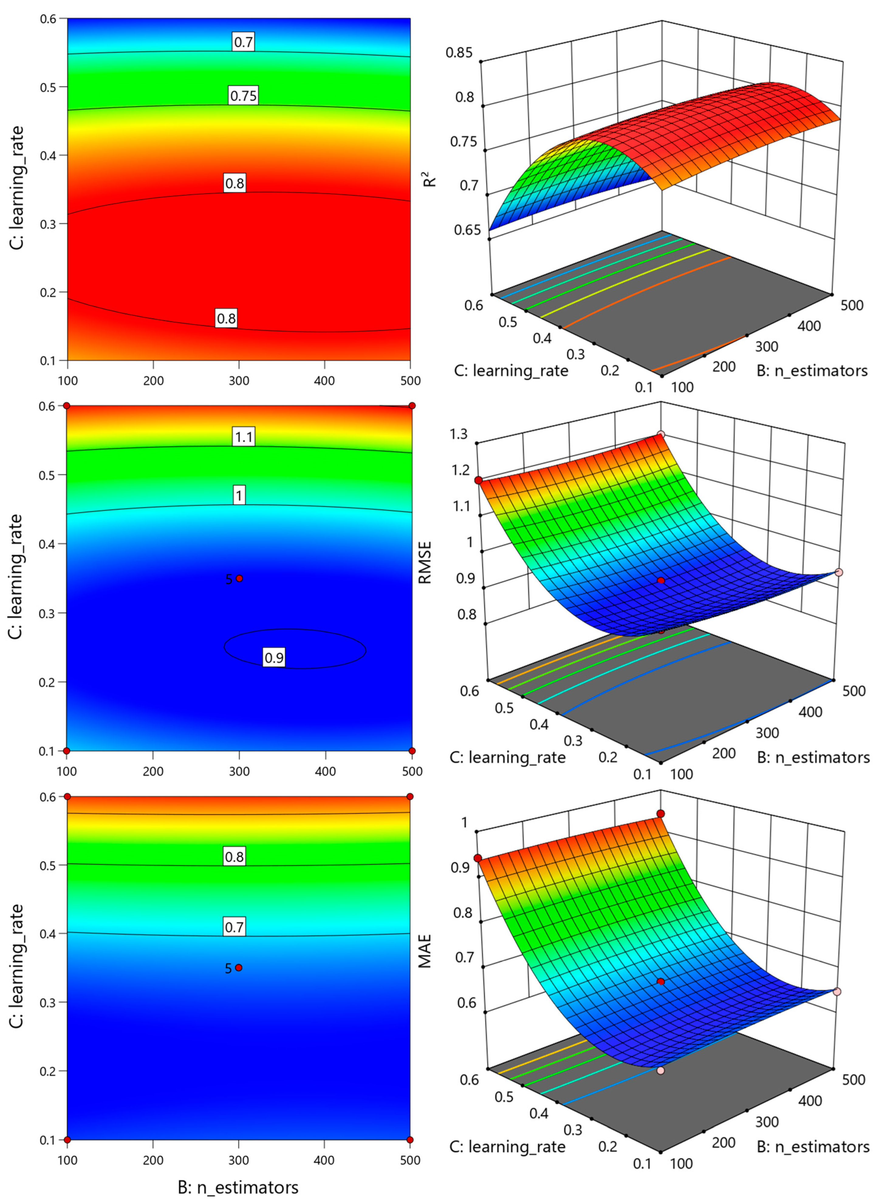
The regression analysis revealed that the C was the most influential hyperparameter affecting model performance, whereas the effects of A and B were comparatively less significant within the investigated ranges. In addition, the quadratic term of C was statistically significant, indicating a pronounced nonlinear response. Among the interaction terms, only the interaction between A and C showed statistical significance, while the remaining interaction effects were weak or insignificant.
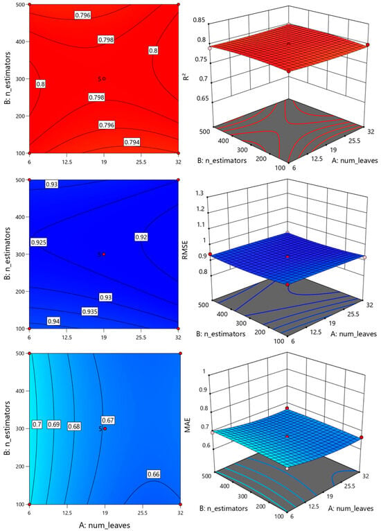
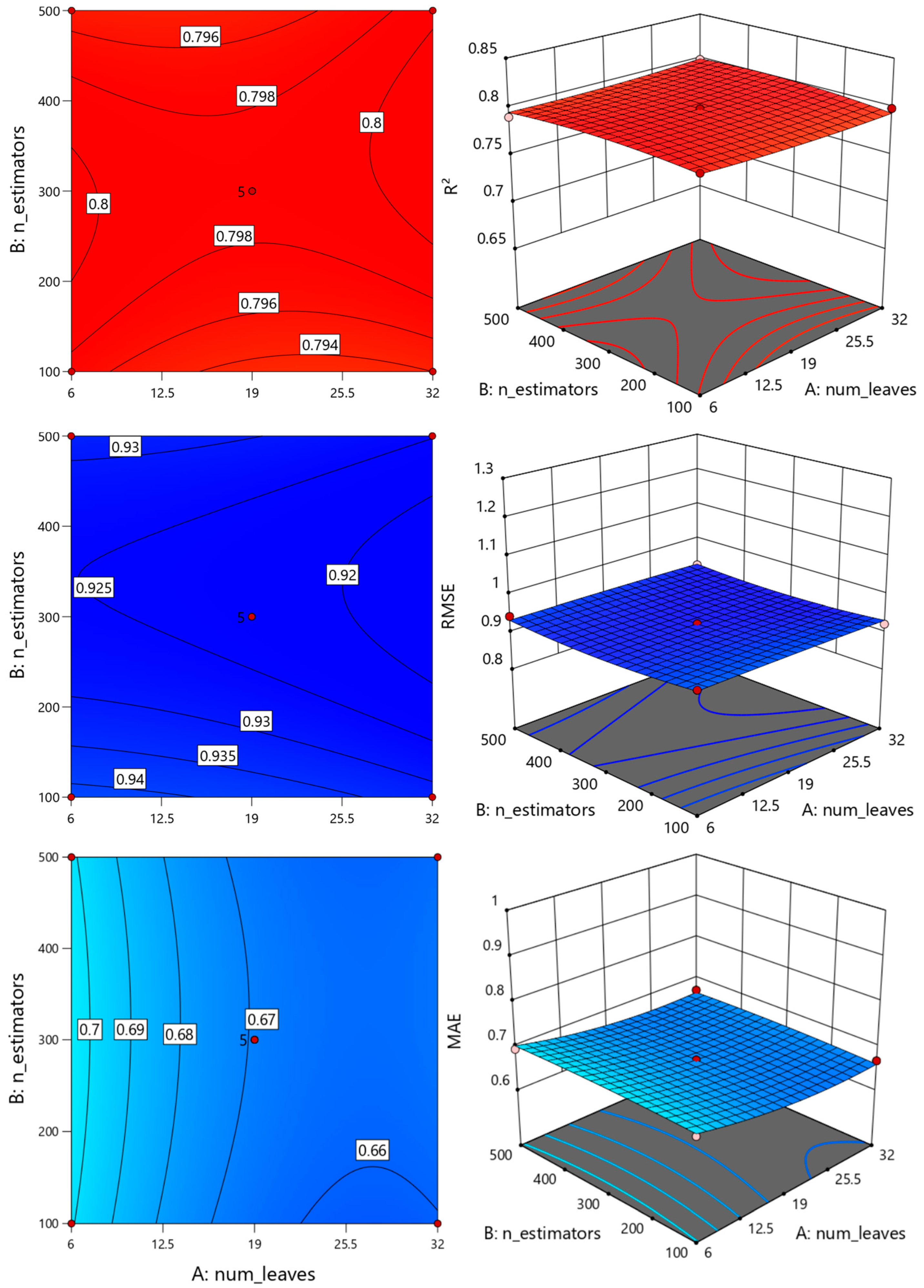
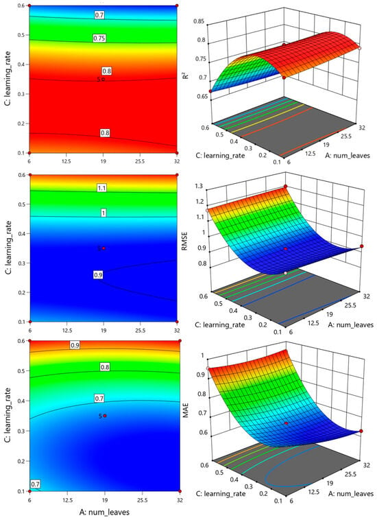
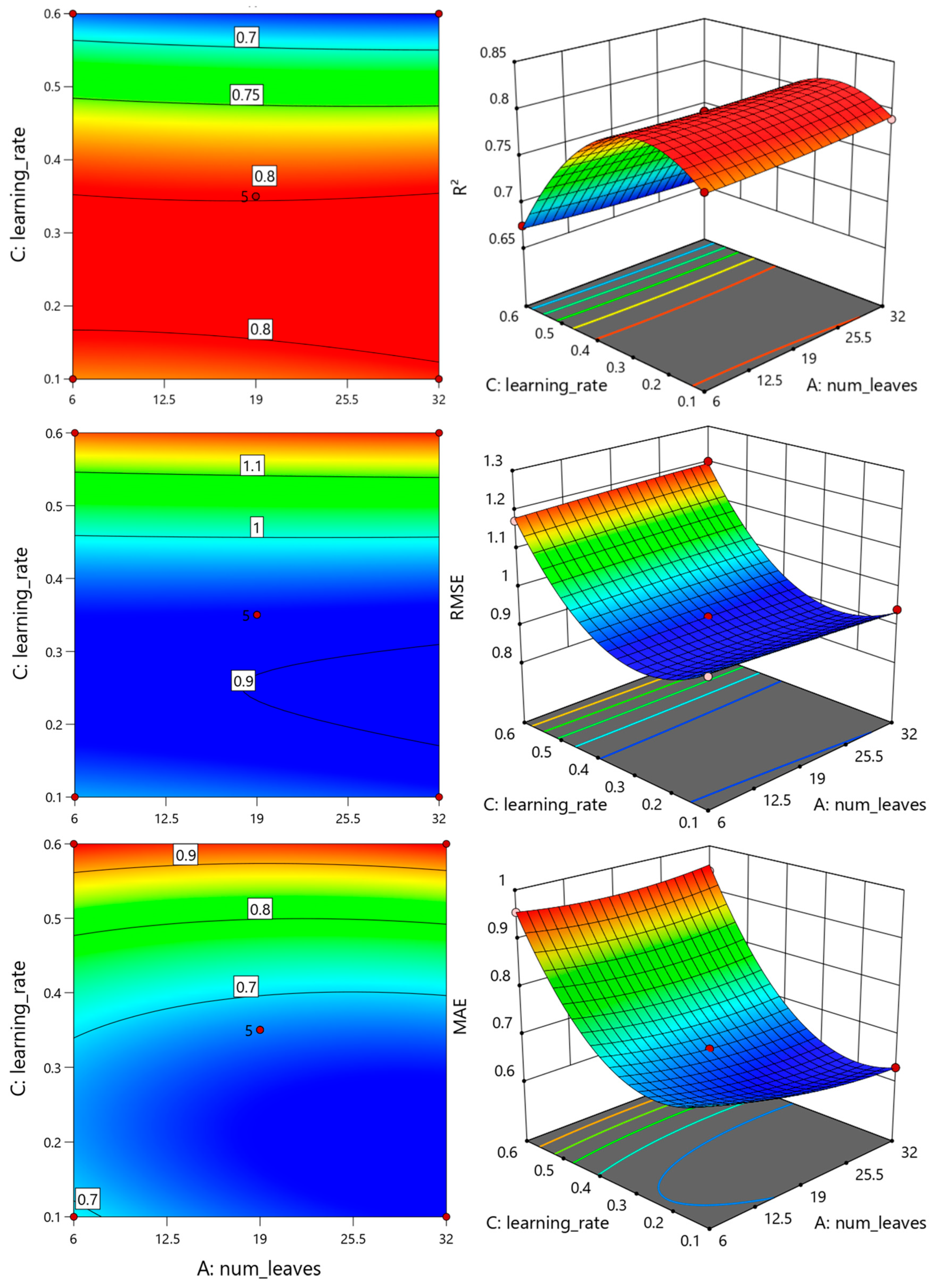
As illustrated in Figure 1, Figure 2 and Figure 3, the response surfaces were relatively flat along the A and B directions but exhibited substantial curvature along the C axis. Increasing the learning rate from a low level to a moderate level improved model performance, as evidenced by higher R2 values and lower RMSE and MAE values. However, further increases in the learning rate led to a deterioration in model performance. This trend suggests that the predictive capability of the model was primarily governed by the learning rate rather than by strong interactions among the investigated hyperparameters.
Figure 1.
Response surface plots of the three response values (R2, RMSE, and MAE) with respect to A and B.
Figure 2.
Response surface plots of the three response values with respect to A and C.
Figure 3.
Response surface plots of the three response variables with respect to B and C.
Because the replicated centre-point runs were obtained from deterministic model evaluations conducted under a fixed random seed, the resulting F-values and p-values should be interpreted qualitatively rather than as strict measures of statistical significance. Therefore, the primary value of the RSM in this study lies not in identifying a unique mathematical optimum, but in revealing the overall response patterns, the direction and magnitude of dominant factor effects, and the limited interactions among the investigated hyperparameters. These findings provide a rationale for adopting OED as a more suitable factor-screening strategy for the present optimization problem, which is characterized by a small sample size and a performance landscape dominated by a single influential factor. These findings suggest that OED may offer a more efficient and informative alternative to conventional RSM-based optimization for limited-sample hyperparameter tuning problems, particularly when model performance is governed primarily by a single dominant factor and interaction effects are limited.
2.2. Analysis of Orthogonal Experiment Results
Based on the diagnostic results obtained from the RSM analysis, an L9(33) OED was subsequently employed to further evaluate the effects of factors A, B, and C on R2, RMSE, and MAE. The complete range analysis results for the three-performance metrics are presented in Tables S5–S7, while the corresponding OED analysis of variance (ANOVA) results are summarized in Table S8.
The range analysis consistently demonstrated that the relative importance of the investigated factors followed the order C > B > A for all three performance metrics (R2, RMSE, and MAE), confirming that the C was the most sensitive hyperparameter. Factor C exhibited a pronounced nonlinear effect: increasing C from Level 1 to Level 2 improved model performance by increasing R2 and reducing both RMSE and MAE, whereas a further increase to Level 3 resulted in performance deterioration. In contrast, factors A and B produced only minor variations across all three-evaluation metrics. The OED ANOVA results further confirmed the dominant influence of factor C. The calculated F-values for C were 30.73, 29.12, and 72.69 for R2, RMSE, and MAE, respectively, all exceeding the critical value of F0.05(2,2) = 19.0. By comparison, neither factor A nor factor B exhibited statistically significant effects. These findings are fully consistent with the conclusions drawn from the RSM analysis. However, unlike RSM, the OED approach avoids the potential overestimation of statistical significance caused by near-zero pure error in deterministic model evaluations, thereby providing more robust statistical inference and factor discrimination.
The OED results indicated that A3B3C2 was the optimal factor combination for maximizing R2 and minimizing RMSE, whereas A3B2C1 produced the lowest MAE. Considering the overall performance across all three-evaluation metrics, A3B3C2 was selected as the final parameter combination for further optimization. Subsequently, factors A and B were fixed at their optimal levels (A = 32 and B = 500), and additional experiments were conducted by varying factor C within the range of 0.35–0.60. The optimal configuration was identified as min_child_samples = 2, A = 32, B = 500, and C = 0.50. Under these optimized conditions, the model achieved an R2 of 0.8015, an RMSE of 0.9163, and an MAE of 0.6599 on the independent test dataset.
In summary, the OED approach efficiently identified the dominant hyperparameters governing model performance and generated a near-optimal parameter combination with a limited number of parameter evaluations. Guided by the response trends revealed by RSM, OED provided a more effective and interpretable means of discriminating the relative importance of the investigated hyperparameters under the limited-data conditions considered in this study. Based on the combined RSM and OED analyses, the optimal LightGBM hyperparameter configuration was determined as min_child_samples = 2, num_leaves = 32, n_estimators = 500, and learning_rate = 0.5. Under these optimized conditions, the model achieved an R2 of 0.8015, RMSE of 0.9163, and MAE of 0.6599 on the independent test dataset. Although the optimized model achieved satisfactory predictive performance for the present dataset, the validation results also indicate noticeable variability across different data partitions, which is expected for small experimental datasets. Therefore, the proposed framework should be regarded as a practical decision-support tool rather than a universally applicable predictive model. The proposed RSM–OED-guided optimization framework provides an efficient and interpretable strategy for hyperparameter optimization in machine-learning applications involving limited and heterogeneous experimental datasets. It should be emphasized that the objective of the proposed optimization framework is to improve the performance of a given baseline model rather than to demonstrate superiority over all alternative machine-learning algorithms. The optimized LightGBM exhibited substantial improvements relative to its initial configuration, confirming that statistically guided hyperparameter optimization can effectively enhance model performance. Different machine-learning algorithms possess distinct learning mechanisms; therefore, the optimized performance of one algorithm should not necessarily be interpreted as exceeding that of fundamentally different models.
2.3. Comparison of Optimization Strategies
Table 1 compares the proposed RSM–OED framework with grid search and Bayesian optimization. Although grid search achieved the same fixed-test performance as the OED-guided strategy, it required substantially more candidate model evaluations. Bayesian optimization also produced comparable results within a limited evaluation budget; however, because model performance was primarily governed by C, the surrogate model provided limited additional optimization insight. The results demonstrate that the RSM–OED approach can achieve competitive predictive performance with fewer evaluations while maintaining clear factor-level interpretability. These characteristics make it an efficient and practical hyperparameter optimization strategy for the present limited-sample system.
Table 1.
Comparison of hyperparameter optimization strategies under the fixed split.
2.4. Robustness Validation of the Optimized LightGBM Model
Because the present study was based on a relatively small experimental dataset, the predictive performance of the optimized LightGBM model may be influenced by the choice of training–testing partition. To evaluate its robustness and generalization capability, three complementary validation protocols were employed. The independent 33:9 hold-out test served as the primary benchmark for model selection, while five-fold cross-validation and 100 Monte Carlo repeated hold-out validations (80:20 split) were conducted to quantify the uncertainty associated with different data partitions. Given the limited sample size, each validation subset contained relatively few observations and covered only a restricted response range, potentially leading to considerable variability in the coefficient of determination (R2). Therefore, RMSE and MAE, together with the performance distributions obtained from repeated random partitions, provide a more comprehensive assessment of model robustness under limited-data conditions.
The robustness validation results are summarized in Table 2. The optimized LightGBM model achieved satisfactory predictive performance on the independent hold-out test, with an R2 of 0.8015, RMSE of 0.9163, and MAE of 0.6599. In contrast, five-fold cross-validation and Monte Carlo repeated hold-out validation produced lower average R2 values and greater variability. These differences primarily reflect the limited size and heterogeneous distribution of the experimental dataset rather than deficiencies in the predictive capability of the optimized model. Under such conditions, validation subsets containing only 8–9 observations are highly sensitive to the distribution of individual samples, and a small number of influential observations can substantially affect the calculated R2 values. Consequently, the lower and more variable R2 values should be interpreted as a manifestation of statistical uncertainty associated with limited-data validation rather than poor model quality. Collectively, the complementary validation protocols demonstrate that the optimized LightGBM model provides reliable predictions while explicitly characterizing the uncertainty associated with sparse experimental datasets, thereby improving confidence in its application to SCC process optimization. It should be emphasized that the present work does not claim that LightGBM is inherently superior to other machine-learning algorithms for SCC purification. Instead, the primary contribution lies in demonstrating that a statistically guided optimization framework can substantially improve model performance while simultaneously enhancing interpretability and optimization efficiency.
Table 2.
Robustness validation of the optimized LightGBM model under different validation protocols.
2.5. Model Interpretability and Process-Variable Importance
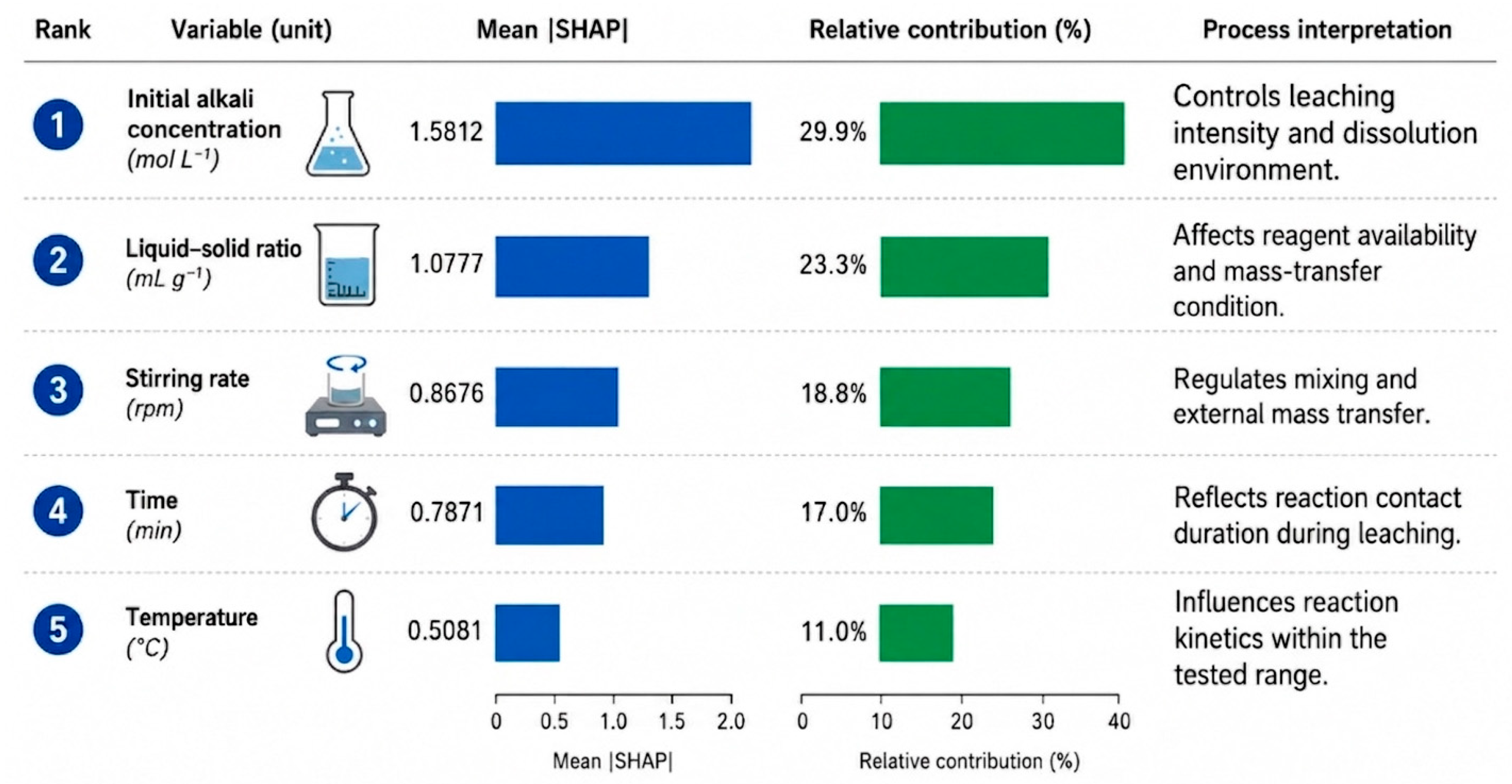
To move beyond purely numerical model optimization and gain mechanistic insights into the prediction process, SHAP analysis was performed to quantify the contributions of individual operating variables to the optimized LightGBM model. SHAP values represent the average marginal contribution of each input variable to model predictions, with larger mean absolute SHAP (|SHAP|) values indicating a greater influence on the predicted carbon content of SCC leaching residues. As summarized in Figure 4, the analysis integrates variable ranking, quantitative contribution, and engineering interpretation to provide a comprehensive understanding of the factors governing SCC purification.
Figure 4.
SHAP-based interpretation of the optimized LightGBM model for predicting the carbon content of SCC leaching residues. The figure presents the ranking of the five operating variables according to their mean absolute SHAP (|SHAP|) values, together with their relative contributions to model predictions and corresponding engineering interpretations.
Initial alkali concentration was identified as the most influential process variable, with a mean |SHAP| value of 1.5812, accounting for 29.9% of the total contribution. This result indicates that alkali dosage plays the dominant role in controlling the leaching environment and the dissolution of metal impurities, thereby directly influencing the carbon purity of the leaching residue. The liquid–solid ratio ranked second (|SHAP| = 1.0777, 23.3%), reflecting its importance in regulating reagent availability and solid–liquid contact, both of which strongly affect mass-transfer conditions during alkaline leaching.
Stirring rate was the third most influential variable (|SHAP| = 0.8676, 18.8%), highlighting the importance of hydrodynamic conditions in promoting external mass transfer and reducing diffusion limitations. Leaching time contributed 17.0% (|SHAP| = 0.7871), indicating that sufficient reaction time is required to achieve effective impurity dissolution and reaction completion. In contrast, temperature exhibited the smallest contribution (|SHAP| = 0.5081, 11.0%) within the investigated operating range, suggesting that its influence on carbon purification was secondary compared with chemical dosage and hydrodynamic conditions.
The engineering interpretation presented in Figure 4 demonstrates that each operating variable influences carbon purification efficiency through a distinct physicochemical mechanism. Initial alkali concentration primarily controls leaching intensity and the dissolution environment, whereas the liquid–solid ratio governs reagent availability and the efficiency of solid–liquid mass transfer. Stirring rate enhances mixing and external mass transfer, while leaching time determines the duration of reagent–solid contact and the extent of dissolution reactions. Although temperature affects reaction kinetics, its contribution is comparatively limited under the investigated conditions.
These findings establish a direct link between the data-driven predictions of the optimized LightGBM model and the underlying chemical engineering principles governing SCC purification. More importantly, the SHAP analysis indicates that optimizing reagent utilization and hydrodynamic conditions is likely to produce greater improvements in the carbon purification performance than increasing thermal input alone. Consequently, the proposed explainable ML framework not only enhances model transparency but also provides practical guidance for process optimization, operational control, and cleaner production. By identifying the most influential operating variables, the framework supports more resource-efficient purification and utilization of carbon-containing residues from SCC recycling while reducing unnecessary experimental effort, energy consumption, and chemical usage, thereby contributing to the sustainable recovery of valuable carbon resources from hazardous industrial waste.
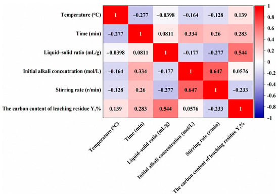
To further analyze the coupling effect between variables, Pearson correlation analysis was used to explore the linear relationship between operating parameters and the carbon content of leaching residues. As illustrated in Figure 5, the liquid-to-solid ratio exhibits the strongest positive correlation with the carbon content of the leaching residues (r = 0.544), indicating that, from a statistical perspective, increasing the liquid-to-solid ratio favors higher carbon retention in the residue. Leaching time also shows a moderate positive correlation with the target variable (r = 0.283). In contrast, stirring rate demonstrates a negative correlation with residual carbon content (r = −0.233), whereas temperature and initial alkali concentration exhibit relatively weak linear associations with the response. Additionally, certain process parameters are interrelated. For instance, a strong positive correlation is observed between initial alkali concentration and stirring rate (r = 0.647), suggesting that the operational variables are not entirely independent and highlighting potential interaction effects within the input parameter system. The observed correlations further suggest that SCC purification behavior is governed by simultaneous equilibrium and transport-related effects rather than by isolated parameter contributions.
Figure 5.
Pearson correlation matrix between input and output variables.
2.6. Implications for Cleaner Production and Resource Recovery
SCC generated during primary aluminium production has traditionally been regarded as a hazardous waste because of the presence of fluoride- and cyanide-bearing compounds. However, SCC also contains significant quantities of graphitic carbon that can be recovered and reused in high-value applications, including battery anodes, graphene materials, silicon carbide production, and metallurgical reductants. Consequently, the challenge is no longer limited to waste detoxification but extends to maximizing resource recovery while minimizing environmental impacts throughout process development. Such an approach is consistent with the principles of cleaner production and the circular economy, which emphasize waste valorization, efficient resource utilization, and minimization of material losses [34,35,36].
Conventional optimization of SCC purification generally relies on repeated laboratory experiments involving numerous combinations of operating variables, including alkali concentration, liquid–solid ratio, temperature, leaching time, and stirring rate. Although effective, this trial-and-error strategy is resource-intensive, requiring substantial consumption of chemicals, water, energy, and analytical effort while generating additional hazardous laboratory waste. Improving optimization efficiency is therefore an important component of cleaner production because it reduces resource consumption during process development rather than only improving the final operating conditions [37].
To illustrate the practical implications of the proposed framework, Table 3 summarizes its performance from both optimization and sustainability perspectives. In addition to prediction accuracy, the comparison considers optimization efficiency, interpretability, and potential contributions to cleaner production, thereby providing a broader assessment of its engineering value.
Table 3.
Comparison of different hyperparameter optimization strategies from machine-learning and cleaner production perspectives.
As summarized in Table 3, the proposed RSM–OED-guided optimization achieved predictive performance comparable to exhaustive grid search while substantially reducing the number of parameter evaluations and providing improved engineering interpretability. Compared with the 64 candidate parameter combinations evaluated by grid search, this represents an approximate 86% reduction in the primary search space, substantially improving optimization efficiency without sacrificing prediction accuracy. Although Bayesian optimization achieved similar predictive performance using a comparable number of evaluations, it provided considerably less information regarding the relative importance of individual hyperparameters. In contrast, the OED simultaneously identified the dominant factors governing model performance, thereby improving both optimization efficiency and engineering interpretability. For larger datasets, the overall workflow remains applicable, whereas the hyperparameter search strategy and model complexity may require adjustment to balance prediction accuracy and computational efficiency. Larger datasets may also enable the incorporation of more advanced optimization algorithms and external validation procedures.
It should be emphasized that the reduction reported in Table 3 refers to optimization effort rather than laboratory experimentation directly. Nevertheless, more efficient optimization frameworks have important practical implications for experimental process development. Reliable predictive models can reduce the number of verification experiments required during process optimization, thereby lowering reagent consumption, water usage, analytical workload, laboratory operating time, and the generation of secondary hazardous wastes. Rather than directly reducing chemical consumption during a single alkaline-leaching experiment, the primary advantage of the proposed framework lies in reducing the number of trial-and-error experiments required for process optimization. Compared with conventional empirical optimization strategies, the data-driven workflow can rapidly identify promising operating conditions, thereby decreasing unnecessary experimental iterations, reagent consumption associated with repeated laboratory tests, and overall optimization time. From an optimization perspective, conventional one-factor-at-a-time experimentation generally requires a large number of repeated laboratory tests before approaching satisfactory operating conditions. In contrast, the proposed framework establishes a predictive model after the initial experimental dataset has been obtained, allowing subsequent process optimization to be performed computationally. Consequently, each additional optimization cycle can be completed without conducting a full set of new laboratory experiments, which is expected to substantially reduce reagent usage, laboratory effort, and energy consumption associated with repeated experimental campaigns. Such improvements align closely with cleaner production strategies, which seek to prevent pollution and minimize resource consumption throughout the production lifecycle rather than relying solely on end-of-pipe treatment technologies.
Beyond improving optimization efficiency, the proposed framework enhances process understanding through explainable artificial intelligence. Machine-learning models are often criticized for their limited interpretability, restricting their application in industrial decision-making. By integrating SHAP analysis, the present study provides quantitative interpretation of the contribution of each operating variable to carbon recovery prediction [38,39]. The SHAP results demonstrated that initial alkali concentration was the dominant factor influencing carbon purification efficiency, followed by liquid–solid ratio, stirring rate, and leaching time, whereas temperature contributed comparatively less within the investigated operating range. These findings agree well with the underlying physicochemical mechanisms governing alkaline leaching. Alkali concentration directly controls impurity dissolution, while liquid–solid ratio and stirring rate primarily influence reagent availability, mass transfer efficiency, and solid–liquid contact. Consequently, optimization strategies should prioritize improving reagent utilization efficiency and hydrodynamic conditions rather than relying primarily on increased thermal input. Such mechanistic interpretation enables engineers to allocate optimization efforts toward the variables with the greatest influence on resource recovery, thereby improving both process efficiency and resource utilization.
The integration of statistical experimental design with explainable ML also demonstrates the feasibility of developing reliable predictive models from relatively small experimental datasets. Small datasets are common in hazardous waste recycling because large-scale experimentation is often constrained by safety requirements, material availability, and economic considerations. Conventional machine-learning optimization methods frequently require large quantities of data to achieve satisfactory generalization, whereas the hybrid framework proposed in this study combines response surface methodology, OED, and explainable ML to maximise the information extracted from limited experiments. Such approaches are increasingly recognised as effective strategies for accelerating sustainable process development under data-constrained conditions [40,41].
From a circular economy perspective, the significance of this work extends beyond SCC purification. Modern circular economy strategies advocate maintaining the highest possible value of materials by recovering secondary resources rather than disposing of industrial wastes [34,36]. By enabling more accurate prediction of carbon purification performance, the proposed framework supports improved utilization of SCC as a secondary carbon resource while reducing uncertainty during process optimisation and scale-up. More efficient process development may ultimately reduce operational costs, improve resource productivity, and increase the economic attractiveness of SCC recycling.
Furthermore, the methodology developed in this study is not restricted to SCC treatment. Many industrial and metallurgical waste streams—including spent lithium-ion batteries, red mud, fly ash, steelmaking slags, copper smelting residues, electronic waste, and mine tailings—are characterised by similarly complex nonlinear relationships between operating variables and resource recovery efficiency while also suffering from limited experimental datasets. The integration of explainable ML with statistical optimization therefore provides a transferable decision-support framework capable of accelerating process optimisation across a broad range of waste valorisation technologies. As digitalisation and intelligent manufacturing continue to advance, explainable artificial intelligence is expected to play an increasingly important role in supporting adaptive process optimisation, digital twins, and sustainable resource management within future circular manufacturing systems [42].
Overall, the proposed framework extends beyond predictive modelling by providing an interpretable, resource-efficient, and scalable methodology for hazardous waste recycling. By integrating explainable ML, statistical experimental design, and engineering interpretation, it supports evidence-based decision-making while reducing optimisation effort and promoting cleaner production. The framework therefore represents a practical pathway toward intelligent resource recovery systems capable of maximising material value while minimising environmental impacts, thereby contributing to the broader transition towards a circular economy.
2.7. Potential Industrial Deployment
Although the present framework was developed using laboratory-scale experimental data, its computational architecture is readily extendable to industrial process optimization. Once process variables (e.g., temperature, liquid-to-solid ratio, alkali concentration, and stirring intensity) are continuously collected through industrial sensors or distributed control systems (DCS), the optimized machine-learning model can be embedded into a real-time decision-support platform to provide rapid prediction of carbon content under different operating conditions.
Furthermore, the proposed framework has the potential to serve as a computational module within future digital twin systems for alkaline-leaching processes. In such applications, the machine-learning model could be continuously updated using newly acquired production data, enabling online prediction, parameter recommendation, and process optimization. Nevertheless, additional validation using pilot-scale and industrial datasets is required before practical deployment.
2.8. Study Limitations and Future Work
From a modelling perspective, fixing the feedstock composition enables the influence of operating variables to be quantified without interference from raw-material variability. This strategy is particularly appropriate for mechanism-oriented process optimization because it allows the relative importance of individual operating parameters to be interpreted more reliably. Nevertheless, the resulting model should be regarded as feedstock-specific rather than universally applicable across different SCC sources.
The present study was based on a relatively small experimental dataset derived from a single SCC source, which may limit the generalizability of the optimized model to other feedstocks and industrial operating conditions. The relatively large variation observed among different validation strategies reflects the intrinsic limitation of modelling based on a small experimental dataset rather than instability of the proposed optimization framework itself. Although robustness was evaluated using cross-validation and Monte Carlo resampling, additional validation with larger and more diverse datasets is required to further assess model transferability. Future studies should incorporate experimental data from different SCC sources and operating environments, investigate additional process variables, and evaluate the applicability of the proposed framework at pilot and industrial scales. Such efforts would further improve the robustness, scalability, and practical implementation of explainable ML for hazardous waste recycling and sustainable resource purification.
3. Experimental Materials and Methodology
3.1. Dataset
The dataset used in this study was derived from the alkaline leaching experiments reported by Yuan et al. [17]. According to the original study, all 42 experiments were conducted using the same homogenized batch of SCC collected from an aluminum smelter in Henan Province, China. Prior to leaching, the SCC was crushed, ground, sieved (<100 mesh), thoroughly mixed, and dried to minimize compositional heterogeneity among experimental runs. The leaching experiments employed analytical-grade NaOH, deionized water, and HCl. The dataset includes five process variables: temperature (40–80 °C), leaching time (30–150 min), liquid–solid ratio (4–8 mL g−1), initial alkali concentration (0.2–1.0 mol L−1), and stirring rate (100–500 rpm). The target variable was the carbon content of the leaching residue, determined by the weight-loss-on-ignition method (Equation (1)).
where is the carbon content of the leaching residue (%), is the ash mass of the residue after being ignited in air at 800 °C for 4 h (g), and is the mass of the residue before ignition.
It should be noted that the present model was established based on a single homogenized SCC feedstock rather than multiple SCC sources with different physicochemical properties. Therefore, the proposed framework is intended to predict the influence of operating conditions under a fixed feedstock condition instead of serving as a universally applicable model for all SCC materials. Extension of the framework to SCC originating from different smelters or operating histories would require additional feedstock descriptors, such as initial carbon content, ash content, fluoride content, mineralogical composition, particle-size distribution, and source information, as additional model inputs. In addition, the present work did not introduce a new analytical method for carbon determination but employed the published experimental values as the target variable for machine-learning modelling. Therefore, the reliability of the carbon-content measurements is inherently associated with the analytical procedure established in the original experimental study.
3.2. Model Selection and Data Partitioning
3.2.1. Training–Testing Split Evaluation
Key evaluation metrics were selected to comprehensively assess model prediction accuracy and generalization ability: Coefficient of determination (R2) measures the model’s ability to explain the variance in the data. Its maximum value is 1, with values closer to 1 indicating better predictive performance. Root mean square error (RMSE) reflects the average deviation between predicted and actual values. A smaller value indicates higher prediction accuracy. Mean absolute error (MAE) measures the average magnitude of prediction errors. A smaller value indicates more stable predictive performance. The calculation formulas are displayed in equations from (S1) to (S3) [43] in the Supplementary Material.
Among the models, GBDT improves predictive performance by sequentially adding weak learners (typically regression trees) using a gradient boosting strategy, where each new tree is trained to fit the residuals of the previous model. In contrast, RF employs a bagging approach that constructs multiple independent DTs through random sampling of data and features, and combines their outputs through averaging, resulting in strong robustness against overfitting. Building upon these ensemble learning methods, XGBoost enhances GBDT by incorporating regularization, second-order gradient optimization, and sparse-aware algorithms, thereby improving both computational efficiency and model generalization. LightGBM further optimizes the GBDT framework from an engineering perspective by introducing gradient-based one-side sampling (GOSS) and exclusive feature bundling (EFB), which reduce data volume and feature dimensionality, significantly accelerating model training. CatBoost, meanwhile, addresses target leakage and categorical feature processing through its ordered boosting mechanism, leading to improved model stability and prediction accuracy [44,45,46,47,48]. To prevent overfitting during model training, the dataset was divided into training and testing sets using ratios of 8:2, 7:3, 6:4, and 5:5 under the default parameter settings of the six models. Random seeds corresponding to each split ratio were applied, rather than using a conventional 9:1 split, to identify the most suitable ratio for optimal predictive performance.
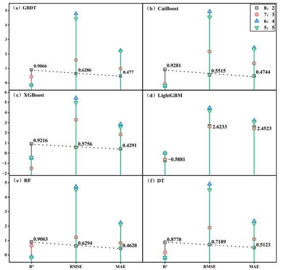
Figure 6 presents a comparison of the evaluation metrics (R2, RMSE, and MAE) for the six models under the four different data split ratios with default parameters. Based on a comprehensive assessment of these three metrics across all models and split ratios, only the LightGBM model did not achieve its best performance at the 4:1 (8:2) training-to-testing ratio. The other five models all showed their best predictive performance at this ratio. Under the default parameter settings with a 4:1 training-to-testing split, the R2 for LightGBM was negative, whereas the other five models achieved R2 values exceeding 0.8, along with relatively low RMSE and MAE values. The poor performance of LightGBM (negative R2) indicates that its default hyperparameter settings are not well suited to the present dataset. Nevertheless, LightGBM was selected for further investigation because of its high flexibility and well-established sensitivity to hyperparameter optimization. Previous studies have shown that, when appropriately tuned, LightGBM often achieves excellent predictive performance and strong generalization ability, particularly for nonlinear problems involving limited datasets. Therefore, the dataset was partitioned using the 4:1 training–testing ratio, and systematic hyperparameter optimization was subsequently performed to fully evaluate the potential of the LightGBM model. LightGBM was selected as a representative case to demonstrate the proposed optimization framework rather than to establish its universal superiority over other machine-learning algorithms.
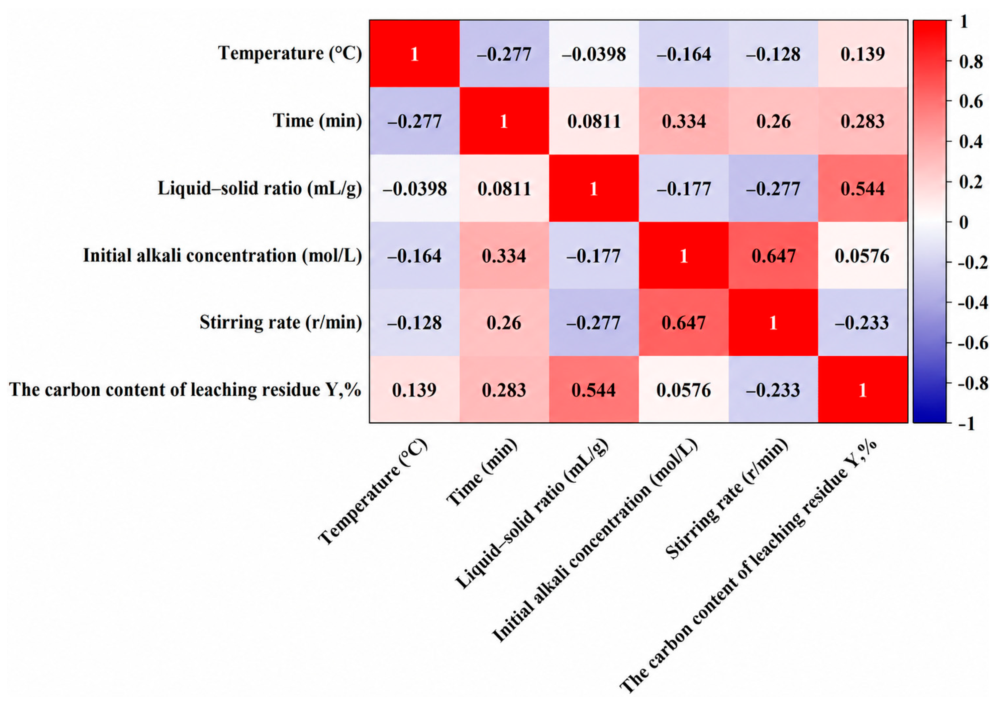
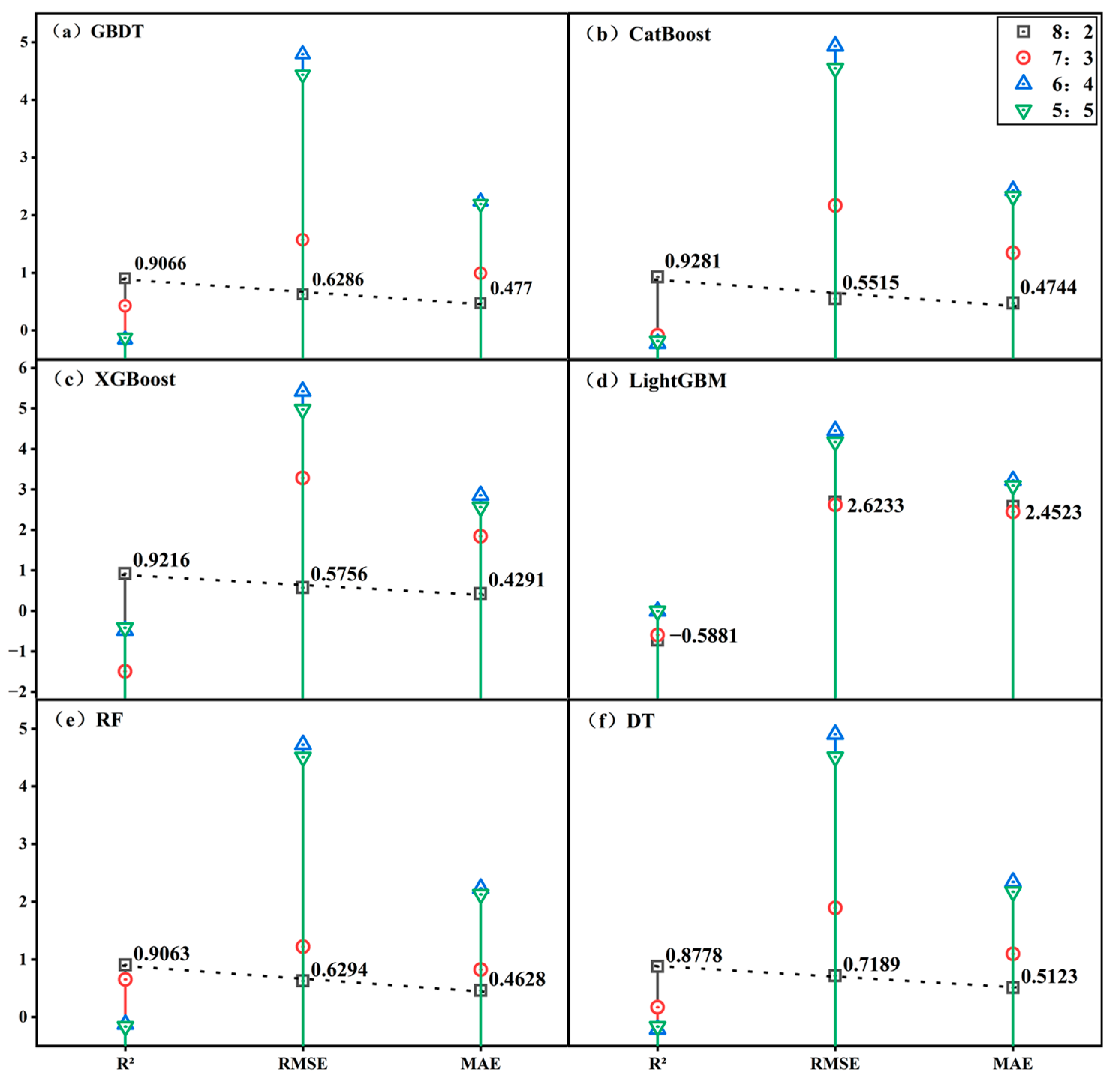
Figure 6.
Comparison of the predictive performance of six ML models under different training–testing split ratios: (a) GBDT; (b) CatBoost; (c) XGBoost; (d) LightGBM; (e) RF; (f) DT.
3.2.2. Dataset Partitioning
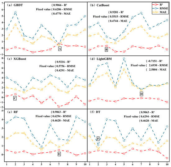
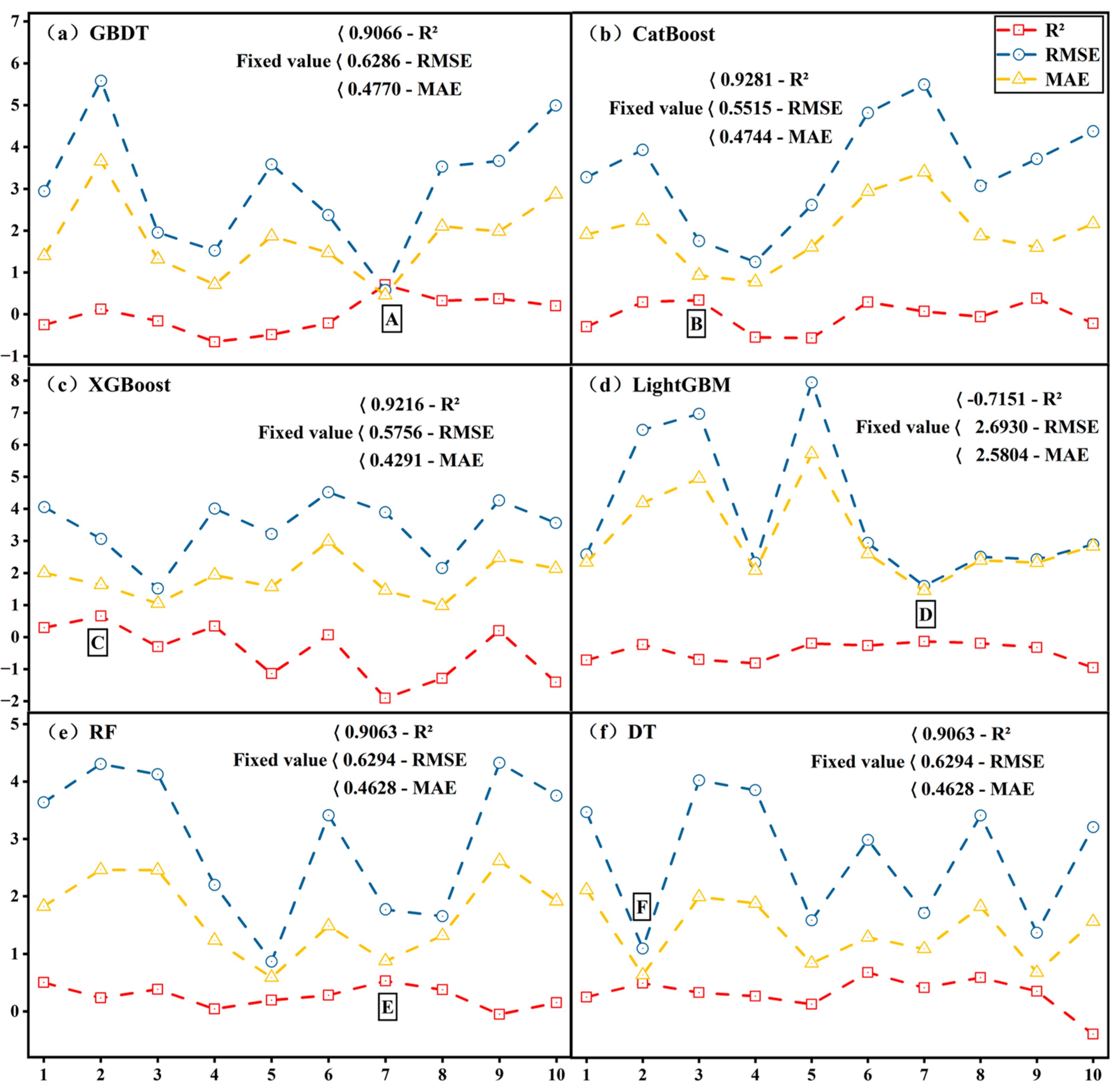
Based on the results in Section 3.2.1, the dataset was divided into training and testing sets using a 4:1 ratio. Figure 7 presents the variation in R2, RMSE, and MAE across ten runs for the six models under unfixed random seeds, where points A–F represent the best performance achieved by each model. Except for LightGBM, the best results obtained under unfixed random seeds were generally inferior to those achieved using a fixed seed. Although LightGBM occasionally showed improved performance under certain random partitions, its overall predictive capability remained the weakest among the six models due to unsuitable default hyperparameter settings. Therefore, a fixed random seed was adopted to ensure data consistency and facilitate subsequent parameter optimization. The dataset was ultimately divided into a training set (33 samples) and a test set (9 samples), and the LightGBM model was further optimized. The results demonstrated that the OED-guided optimization strategy achieved predictive performance comparable to grid search and Bayesian optimization while requiring substantially fewer parameter evaluations, making it an efficient approach for process optimization under limited-data conditions.
Figure 7.
Results of ten repeated experiments on the prediction performance of six models under random seed uncertainty: (a) GBDT; (b) CatBoost; (c) XGBoost; (d) LightGBM; (e) RF; (f) DT.
3.2.3. Robustness Validation and Model Interpretability Analysis
A fixed training–testing split of 33:9 was adopted for model selection and final evaluation. Given the limited dataset size, additional robustness analyses were performed using five-fold cross-validation and 100 Monte Carlo random holdout validations with an 80:20 training–testing split to assess the sensitivity of model performance to data partitioning [40,41,49]. Because each validation fold contained only 8–9 samples and covered a relatively narrow response range, cross-validation R2 values were interpreted with caution. Therefore, greater emphasis was placed on RMSE, MAE, and the distribution of prediction errors from repeated random splits, which provide a more reliable assessment of model robustness and generalization under limited-sample conditions.
To improve model interpretability, Shapley Additive Explanations (SHAP) analysis was applied to the optimized LightGBM model. Based on cooperative game theory, SHAP quantifies the contribution of each input variable to the model output, enabling identification of the most influential process parameters and their effects on the predicted carbon content of SCC leaching residues [38,39].
All ML analyses were performed using Python 3.11. The evaluated models, including GBDT, CatBoost, XGBoost, LightGBM, RF, and DT, were implemented using Scikit-learn (v1.3.0), CatBoost (v1.2.2), XGBoost (v1.7.6), and LightGBM (v4.0.0). Pandas (v2.1.1) and NumPy (v1.26.5) were used for data preprocessing and numerical computation, Matplotlib (v3.8.0) was employed for data visualization, and SHAP (v0.43.0) was used to interpret the optimized LightGBM model by quantifying the contributions of individual process variables to carbon-content prediction. To facilitate reproducibility, the random seed was fixed to 42 throughout data partitioning, model training, and hyperparameter optimization unless otherwise specified. In the end, apart from the optimized model hyperparameters, all other parameters were set to the model’s default values. SHAP analysis was performed using the SHAP Python package based on the optimized model without additional post-processing.
3.3. Adjustable Hyperparameter Selection
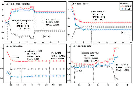
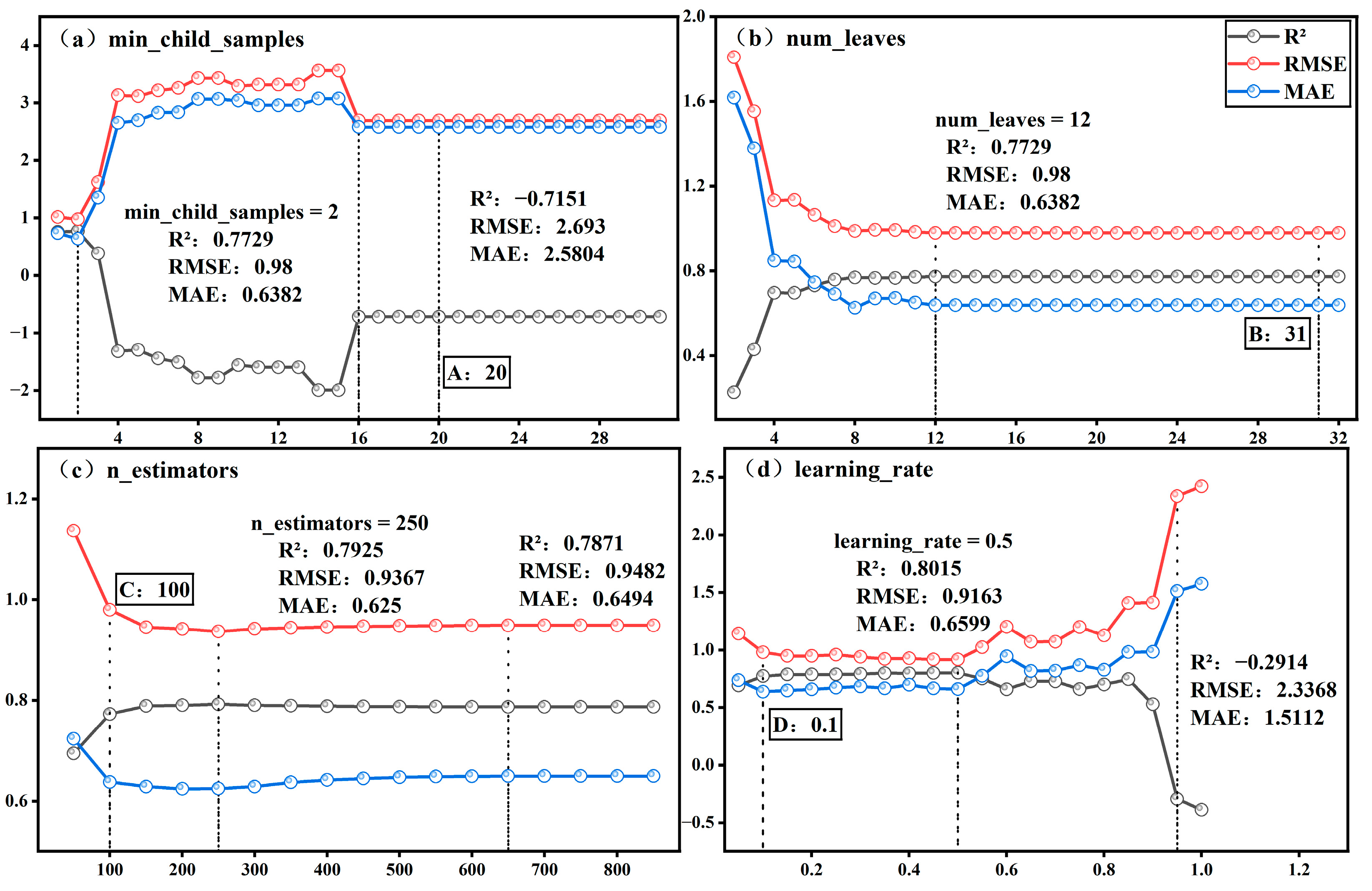
The hyperparameter min_child_samples (minimum number of samples required in a leaf node) takes integer values greater than 1, with a default value of 20. Figure 8a shows the variation in R2, RMSE, and MAE when min_child_samples is adjusted while all other parameters remain at their default settings. At the default value of 20, the model exhibits poor performance (R2 = −0.7151, RMSE = 2.693, MAE = 2.5804), indicating severe underfitting. As min_child_samples decreases from 20 to 1–2, prediction accuracy improves markedly, reaching optimal performance at min_child_samples = 2 (R2 = 0.7729, RMSE = 0.98, MAE = 0.6382). This suggests that the default value is too large for the present limited-sample dataset, restricting leaf-node splitting and limiting the model’s ability to capture nonlinear relationships. Because min_child_samples exerts a dominant influence on model performance, it was fixed at 2 in subsequent single factor analyses to avoid persistent underfitting that could mask the effects of other parameters. All remaining parameters were retained at their default values, providing a revised baseline for further hyperparameter investigation.
Figure 8.
Effects of four hyperparameters on the R2 of the LightGBM model in single-factor experiments: (a) min_child_samples; (b) num_leaves; (c) n_estimators; (d) learning_rate.
With min_child_samples = 2, the model achieved R2 = 0.7729, RMSE = 0.98, and MAE = 0.6382 on the test set. To further improve predictive performance, three additional hyperparameters were selected for systematic analysis: num_leaves (A), n_estimators (B), and learning_rate (C). These parameters influence the gradient boosting model from different perspectives: A controls the complexity of individual trees, B determines the number of boosting iterations and convergence behavior, and C regulates the step size of each iteration and the contribution of new trees to the overall model update.
Previous studies have shown that num_leaves (A), n_estimators (B), and learning_rate (C) are key hyperparameters influencing the predictive accuracy of LightGBM and other gradient boosting models [50]. Variations in these parameters directly affect model fitting and generalization performance. Therefore, they were selected for response surface and orthogonal experimental analyses. Figure 8b–d present the corresponding R2, RMSE, and MAE values under single-factor conditions with min_child_samples fixed at 2. The hyperparameter A takes integer values ≥ 2 with a default value of 31; B takes integer values ≥ 1 with a default value of 100; and C takes positive real values with a default value of 0.1. As shown in Figure 8b, the model achieves its highest prediction accuracy at A = 12 (R2 = 0.7729, RMSE = 0.98, and MAE = 0.6382). However, model performance remains relatively stable when A exceeds 12, including at the default value (31). Figure 8c shows that default B = 100 yields lower predictive performance than B = 250, while the model performance gradually stabilizes when the value exceeds 650. Figure 8d indicates that the optimal C is 0.5, achieving R2 = 0.8015, RMSE = 0.9163, and MAE = 0.6599, whereas the default value (0.1) is suboptimal. When C exceeds 0.95, model underfitting becomes apparent. Overall, among the three hyperparameters, only A achieves near-optimal values of R2, RMSE, and MAE at its default setting (31), whereas B and C reach their optimal performance at non-default values. These results indicate that further optimization using response surface methodology and OED is necessary.
3.4. Hyperparameter Optimization Methodology
To achieve efficient optimization of key parameters in the LightGBM model, this study introduces RSM and OED to systematically analyze and optimize the model hyperparameters.
3.4.1. Response Surface Methodology for Optimizing Hyperparameters
RSM is a statistical optimization approach that uses designed experiments and regression analysis to evaluate the effects of multiple factors and their interactions on a response variable [51]. The relationship between hyperparameters and model performance was described using a quadratic polynomial model, expressed in Equation (2) as follows:
where Y represents the variable, denotes the influencing factors, and represents the regression coefficients. The significance of the model is evaluated using ANOVA. By combining three-dimensional response surface plots and contour plots, the effects of individual factors and their interactions on the response can be visualized intuitively, allowing the identification of optimal parameter regions. RSM is particularly suitable for optimization problems involving strong multi-factor coupling and nonlinear relationships between variables and responses.
To systematically evaluate the effects of key LightGBM hyperparameters on predictive performance, a three-factor, three-level Box–Behnken response surface design was employed and displayed in Table 4. The independent variables were num_leaves (A), n_estimators (B), and learning_rate (C), each assigned three coded levels (−1, 0, and 1) corresponding to low, medium, and high values, respectively [52]. Factor levels were selected based on the parameter ranges identified in Section 3.3. The response variables were R2, RMSE, and MAE, and a quadratic polynomial model was established and evaluated using ANOVA.
Table 4.
Box–Behnken experimental factor level table.
3.4.2. Optimization of Hyperparameters Using OED
OED is a multi-factor optimization method based on orthogonal arrays that enables the evaluation of multiple factors with a limited number of experiments while maintaining balanced experimental information. By selecting appropriate orthogonal arrays (e.g., L9 and L16), factor effects can be efficiently assessed using range analysis and ANOVA. Because OED does not rely on functional model fitting, it is particularly suitable for systems with multiple factors and weak interactions.
To optimize the LightGBM hyperparameters, A, B, and C were selected based on Section 3.3. The response variables were R2, RMSE, and MAE. A three-factor, three-level (33) orthogonal experiment was designed using the same factor levels as those adopted in the response surface analysis (Table 5).
Table 5.
Orthogonal experiment factors and levels.
In this study, RSM was first used to characterize the LightGBM hyperparameter-response space, followed by OED for parameter optimization. The effectiveness of OED was further evaluated against grid search and Bayesian optimization within the same hyperparameter domain. Prediction accuracy and the number of evaluated candidate configurations were used as indicators of model performance and search efficiency [53,54,55,56]. The objective was to examine whether the OED-guided strategy could achieve competitive predictive performance while maintaining superior factor-level interpretability and reduced computational requirements.
4. Conclusions
This study developed an explainable machine learning framework for predicting the carbon content of SCC leaching residues under limited-data conditions. Six widely used machine learning algorithms (GBDT, CatBoost, XGBoost, LightGBM, RF, and DT) were systematically evaluated, and LightGBM was selected for further optimization. By integrating RSM, OED, and local parameter refinement, an efficient and interpretable hyperparameter optimization strategy was established. In addition, robustness validation and SHAP analysis were incorporated to improve model reliability and interpretability.
Systematic hyperparameter optimization substantially improved the predictive capability of the LightGBM model. The optimized model, with min_child_samples = 2, num_leaves = 32, n_estimators = 500, and learning_rate = 0.5, achieved an R2 of 0.8015, RMSE of 0.9163, and MAE of 0.6599 on the independent test dataset. Compared with conventional grid search, the proposed RSM–OED-guided strategy achieved comparable predictive accuracy while requiring substantially fewer parameter evaluations and providing improved insight into the relative importance of individual hyperparameters. Robustness analyses further demonstrated that the observed variability in repeated validation primarily reflected the statistical uncertainty associated with limited experimental data rather than deficiencies in the optimized model.
SHAP analysis revealed that initial alkali concentration, liquid–solid ratio, stirring rate, and leaching time were the dominant process variables governing carbon purification efficiency, whereas temperature exerted a comparatively smaller influence within the investigated operating range. These findings indicate that improving reagent utilization and hydrodynamic conditions offers greater potential for enhancing carbon purification efficiency than increasing thermal input alone. By combining statistical experimental design with explainable artificial intelligence, the proposed framework not only improves prediction accuracy but also enhances process understanding, reduces optimization effort, and supports cleaner production through more resource-efficient process development.
Although the proposed framework provides an effective data-driven tool for assisting process optimization under limited-data conditions, further validation using larger and more diverse datasets is still required before broader industrial application. Future work should validate the framework using larger and more diverse datasets collected from different aluminium smelters and evaluate its applicability to other hazardous waste recycling and resource purification processes. Overall, the proposed explainable machine learning framework provides an efficient, interpretable, and transferable decision-support tool for optimizing hazardous waste recycling processes under limited-data conditions, contributing to cleaner production and the sustainable purification of valuable carbon resources.
Supplementary Materials
The following supporting information can be downloaded at https://www.mdpi.com/article/10.3390/recycling11080148/s1, Table S1: Analysis of R2, RMSE, and MAE based on the Box–Behnken experimental design; Table S2: Regression equation validation of R2 based on the Box–Behnken experimental design; Table S3: Regression equation validation of RMSE based on the Box–Behnken experimental design; Table S4: Regression equation validation of MAE based on the Box–Behnken experimental design; Table S5: Orthogonal experiment R2 range analysis results; Table S6: RMSE range analysis results of orthogonal experiments; Table S7: Range analysis results of orthogonal experiment MAE values; and Table S8: ANOVA results for orthogonal experiments.
Author Contributions
Conceptualization, X.B.; methodology, S.Z. and X.B.; software, S.Z.; validation, S.Z., L.D. and J.S.; formal analysis, S.Z.; investigation, S.Z., J.S. and X.B.; resources, X.B.; writing—original draft preparation, S.Z. and L.D.; writing—review and editing, L.D., M.A.D. and X.B.; visualization, S.Z., L.D. and M.A.D.; supervision, L.D. and X.B.; project administration, X.B.; funding acquisition, X.B. All authors have read and agreed to the published version of the manuscript.
Funding
This study was funded by the National Natural Science Foundation of China, grant number 52204296.
Data Availability Statement
The original contributions presented in this study are included in the article and Supplementary Materials. Further inquiries can be directed to the corresponding author.
Acknowledgments
The authors sincerely acknowledge the support provided by the School of Chemical Engineering and Technology, China University of Mining and Technology; the Western Australian School of Mines, Curtin University, Australia; and the Egyptian Petroleum Research Institute (EPRI), Cairo, Egypt, for their invaluable institutional, administrative, and editorial support throughout this work.
Conflicts of Interest
The authors declare no conflicts of interest.
References
- Mathaba, M.; Banza, J. Application of machine learning approach (artificial neural network) and shrinking core model in cobalt (II) and copper (II) leaching process. J. Environ. Sci. Health A Tox Hazard. Subst. Environ. Eng. 2024, 59, 25–32. [Google Scholar] [CrossRef] [Scilit] [PubMed]
- Lv, X.; Sun, X.; Bu, W.; Tan, X.; Zhu, J.; Han, Z. An efficient recycling process of spent cathode carbon blocks via low temperature molten salt roasting and two stage leaching. Sep. Purif. Technol. 2025, 361, 131566. [Google Scholar] [CrossRef] [Scilit]
- Zheng, Z.; Tang, Y.; Yang, Y.; Wu, J.; Jiang, G.; Xue, Y.; Fang, G.; Tan, Z.; Zhang, X.; Zhang, W.; et al. A review on the recycling of aluminum electrolytic spent cathode Carbon: Detoxification mechanisms, recovery processes, and environmental assessment. Sep. Purif. Technol. 2025, 378, 134697. [Google Scholar] [CrossRef] [Scilit]
- Dragan, M.; Marko, H.; Niko, S. Spent potlining utilisation possibilities. Waste Manag. Res. J. A Sustain. Circ. Econ. 2003, 21, 467–473. [Google Scholar] [CrossRef] [Scilit] [PubMed]
- Holywell, G.; Breault, R. An Overview of Useful Methods to Treat, Recover, or Recycle Spent Potlining. JOM 2013, 65, 1441–1451. [Google Scholar] [CrossRef] [Scilit]
- Robshaw, T.J.; Bonser, K.; Coxhill, G.; Dawson, R.; Ogden, M.D. Development of a Combined Leaching and Ion-Exchange System for Valorisation of Spent Potlining Waste. Waste Biomass Valorization 2020, 11, 5467–5481. [Google Scholar] [CrossRef] [Scilit]
- Zhao, H.; Liu, F.; Xie, M.; Liu, W.; Sohn, H.Y. Recycling and utilization of spent potlining by different high temperature treatments. J. Clean. Prod. 2021, 289, 125704. [Google Scholar] [CrossRef] [Scilit]
- Chen, Y.; Li, P.; Bu, X.; Chehreh Chelgani, S.; Kong, Y.; Liang, X. Resource utilization strategies for spent pot lining: A review of the current state. Sep. Purif. Technol. 2022, 300, 121816. [Google Scholar] [CrossRef] [Scilit]
- Yuan, J.; Xiao, J.; Li, F.C.; Wang, B.J.; Yao, Z.; Yu, B.L.; Zhang, L.Y. Co-treatment of spent cathode carbon in caustic and acid leaching process under ultrasonic assisted for preparation of SiC. Ultrason. Sonochem. 2018, 41, 608–618. [Google Scholar] [CrossRef] [Scilit] [PubMed]
- Li, P.; Chen, Y.R.; Zeng, H.; Bu, X.N.; Wang, L.Q.; Liang, X.M. Structure characteristics and adsorption performance of graphene oxide prepared by spent carbon cathode-an ultra-low temperature graphitized carbon material. Environ. Sci. Pollut. Res. 2023, 30, 120515–120527. [Google Scholar] [CrossRef] [Scilit] [PubMed]
- Ren, C.; Lin, L.; Liao, Q.; Zhou, H.; Tian, C.; Wang, H.; Lin, Z. Machine Learning-Driven Inverse Design for Low-Carbon and Cost-Effective Organic Acid Leaching of Spent Ternary Lithium Batteries. Environ. Sci. Technol. 2025, 59, 25950–25959. [Google Scholar] [CrossRef] [Scilit] [PubMed]
- Yuan, J.; Xiao, J.; Tian, Z.; Yang, K.; Yao, Z. Optimization of Spent Cathode Carbon Purification Process under Ultrasonic Action Using Taguchi Method. Ind. Eng. Chem. Res. 2018, 57, 7700–7710. [Google Scholar] [CrossRef] [Scilit]
- Yao, Z.; Xiao, J.; Mao, Q.; Wang, G.; Tang, L.; You, Z.; Zhong, Q. Detoxification and Recovery of Spent Carbon Cathodes via NaOH–Na2CO3 Binary Molten Salt Roasting–Water Leaching: Toward a Circular Economy for Hazardous Solid Waste from Aluminum Electrolysis. ACS Sustain. Chem. Eng. 2020, 8, 16912–16923. [Google Scholar] [CrossRef] [Scilit]
- Yuan, J.; Li, H.; Ding, S. Leaching Kinetics of Aluminum from Alkali-Fused Spent Cathode Carbon Using Hydrochloric Acid and Sodium Fluoride. Processes 2022, 10, 849. [Google Scholar] [CrossRef] [Scilit]
- Wang, C.; Mao, S.; Li, L. Study on ultrasonic leaching and recovery of fluoride from spent cathode carbon of aluminum electrolysis. RSC Adv. 2023, 13, 16300–16310, Correction in RSC Adv. 2023, 13, 18128. [Google Scholar] [CrossRef] [Scilit] [PubMed]
- Zhou, L.; Yao, Z.; Sun, K.; Tian, Z.; Li, J.; Zhong, Q. Methodological Review of Methods and Technology for Utilization of Spent Carbon Cathode in Aluminum Electrolysis. Energies 2024, 17, 4866. [Google Scholar] [CrossRef] [Scilit]
- Yuan, J.; Xiao, J.; Tian, Z.; Yang, K.; Yao, Z.; Yu, B.; Zhang, L. Optimization of purification treatment of spent cathode carbon from aluminum electrolysis using response surface methodology (RSM). Asia Pac. J. Chem. Eng. 2017, 13, e2164. [Google Scholar] [CrossRef] [Scilit]
- Yuan, J.; Ding, S.; Li, H.J. Purification of spent cathode carbon from aluminum electrolysis cells by alkali fusion-acid leaching process. J. Mater. Cycles Waste Manag. 2022, 24, 2608–2619. [Google Scholar] [CrossRef] [Scilit]
- Zhu, Z.; Xu, L.; Han, Z.; Liu, J.; Zhang, L.; Tian, S.; Xu, Y.; Koppala, S. Optimization of response surface methodology (RSM) for defluorination of spent carbon cathode (SCC) in fire-roasting aluminum electrolysis. Miner. Eng. 2022, 182, 107565. [Google Scholar] [CrossRef] [Scilit]
- Lu, K.; Chen, X.; Zhang, J.; Chen, J.; Liu, Z.; Chen, L. Comparison of artificial neural network and response surface methodology prediction in key performance of two-component grout material in shield tunneling. Case Stud. Constr. Mater. 2025, 23, e05020. [Google Scholar] [CrossRef] [Scilit]
- McCoy, J.T.; Auret, L. Machine learning applications in minerals processing: A review. Miner. Eng. 2019, 132, 95–109. [Google Scholar] [CrossRef] [Scilit]
- Mishra, A.K. AI4R2R (AI for Rock to Revenue): A Review of the Applications of AI in Mineral Processing. Minerals 2021, 11, 1118. [Google Scholar] [CrossRef] [Scilit]
- Ji, Y.; Wang, L.; Ren, G.; Xu, T.; Li, X.; Chen, X.; Bu, X.; Sha, J. Evaluation of parametric effects of coal flotation based on boosting modeling method. Physicochem. Probl. Miner. Process. 2024, 60, 196385. [Google Scholar] [CrossRef] [Scilit]
- Chehreh Chelgani, S.; Nasiri, H.; Tohry, A.; Heidari, H.R. Modeling industrial hydrocyclone operational variables by SHAP-CatBoost-A “conscious lab” approach. Powder Technol. 2023, 420, 118416. [Google Scholar] [CrossRef] [Scilit]
- Song, Y.; Yu, X.; Huang, M. A Copper Flotation Concentrate Grade Prediction Method Based on an Improved Extreme Gradient Boosting Algorithm. Appl. Sci. 2025, 15, 11142. [Google Scholar] [CrossRef] [Scilit]
- Salehzadeh Gharaei, R.; Gholami, A.; Khoshdast, H.; Biglari, H. A Multi-Method Machine Learning Framework for Simulating Power Dynamics in an Iron Ore Cone Crusher Plant. Miner. Process. Extr. Metall. Rev. 2025, 46, 783–798. [Google Scholar] [CrossRef] [Scilit]
- Nogueira, A.; Sosa, F.H.B.; Dias, A.C.; Coutinho, J.A.P.; Schaeffer, N. An applied machine learning framework for waste lithium-ion battery leaching with integrated preliminary environmental and economic assessment. Green. Chem. 2026, 28, 277–294. [Google Scholar] [CrossRef] [Scilit]
- Sipper, M. High Per Parameter: A Large-Scale Study of Hyperparameter Tuning for Machine Learning Algorithms. Algorithms 2022, 15, 315. [Google Scholar] [CrossRef] [Scilit]
- Khuri, A.I.; Mukhopadhyay, S. Response surface methodology. WIREs Comput. Stat. 2010, 2, 128–149. [Google Scholar] [CrossRef] [Scilit]
- Yang, K.; Gong, P.; Xin, X.; Tian, Z.; Lai, Y. Purifying spent carbon anode (SCA) from aluminum reduction industry by alkali fusion method to apply for Li-ion batteries anodes: From waste to resource. J. Taiwan Inst. Chem. Eng. 2020, 116, 121–127. [Google Scholar] [CrossRef] [Scilit]
- Zhang, Z.; Tang, J.; Chu, M.; Liu, Z.; Shi, Q.; Wang, M.; Li, F.; Lyu, Q. The Amount Prediction and Optimization of the Returned Ore Generated from Sintering Process Based on SHAP Value and Ensemble Learning. Steel Res. Int. 2023, 94, 2300114. [Google Scholar] [CrossRef] [Scilit]
- Wang, M.; Tang, J.; Chu, M.; Shi, Q.; Zhang, Z. Prediction and optimization of flue pressure in sintering process based on SHAP. Int. J. Miner. Metall. Mater. 2025, 32, 346–359. [Google Scholar] [CrossRef] [Scilit]
- Zhang, J.; Zhang, J.; Zhu, P.; Xu, Z.; Zhang, L. Mechanism-infused machine learning for scattered metal recovery: SHAP decodes multiscale physicochemical drivers in refractory matrices. Green. Chem. 2025, 27, 14564–14576. [Google Scholar] [CrossRef] [Scilit]
- Geissdoerfer, M.; Savaget, P.; Bocken, N.M.P.; Hultink, E.J. The Circular Economy—A new sustainability paradigm? J. Clean. Prod. 2017, 143, 757–768. [Google Scholar] [CrossRef] [Scilit]
- Ghisellini, P.; Cialani, C.; Ulgiati, S. A review on circular economy: The expected transition to a balanced interplay of environmental and economic systems. J. Clean. Prod. 2016, 114, 11–32. [Google Scholar] [CrossRef] [Scilit]
- Kirchherr, J.; Reike, D.; Hekkert, M. Conceptualizing the circular economy: An analysis of 114 definitions. Resour. Conserv. Recycl. 2017, 127, 221–232. [Google Scholar] [CrossRef] [Scilit]
- Glavič, P.; Lukman, R. Review of sustainability terms and their definitions. J. Clean. Prod. 2007, 15, 1875–1885. [Google Scholar] [CrossRef] [Scilit]
- Lundberg, S.M.; Lee, S.-I. A unified approach to interpreting model predictions. In Proceedings of the 31st International Conference on Neural Information Processing Systems, Long Beach, CA, USA, 4–9 December 2017; pp. 4768–4777. [Google Scholar]
- Lundberg, S.M.; Erion, G.; Chen, H.; DeGrave, A.; Prutkin, J.M.; Nair, B.; Katz, R.; Himmelfarb, J.; Bansal, N.; Lee, S.-I. From local explanations to global understanding with explainable AI for trees. Nat. Mach. Intell. 2020, 2, 56–67. [Google Scholar] [CrossRef] [Scilit] [PubMed]
- Cawley, G.C.; Talbot, N.L.C. On Over-fitting in Model Selection and Subsequent Selection Bias in Performance Evaluation. J. Mach. Learn. Res. 2010, 11, 2079–2107. [Google Scholar]
- Varoquaux, G. Cross-validation failure: Small sample sizes lead to large error bars. NeuroImage 2018, 180, 68–77. [Google Scholar] [CrossRef] [Scilit] [PubMed]
- Rai, A. Explainable AI: From black box to glass box. J. Acad. Mark. Sci. 2020, 48, 137–141. [Google Scholar] [CrossRef] [Scilit]
- Park, H.; Bai, C.; Wang, L. A Convolutional Neural Network for Classification of Froth Mobility in an Industrial Flotation Cell. Miner. Process. Extr. Metall. Rev. 2023, 44, 209–217. [Google Scholar] [CrossRef] [Scilit]
- Breiman, L. Random Forests. Mach. Learn. 2001, 45, 5–32. [Google Scholar] [CrossRef] [Scilit]
- Friedman, J.H. Greedy function approximation: A gradient boosting machine. Ann. Stat. 2001, 29, 1189–1232. [Google Scholar] [CrossRef] [Scilit]
- Chen, T.; Guestrin, C. XGBoost: A Scalable Tree Boosting System. In Proceedings of the 22nd ACM SIGKDD International Conference on Knowledge Discovery and Data Mining, San Francisco, CA, USA, 13–17 August 2016; pp. 785–794. [Google Scholar]
- Ke, G.; Meng, Q.; Finley, T.; Wang, T.; Chen, W.; Ma, W.; Ye, Q.; Liu, T.-Y. LightGBM: A Highly Efficient Gradient Boosting Decision Tree. In Proceedings of the Neural Information Processing Systems, Long Beach, CA, USA, 4–9 December 2017. [Google Scholar]
- Ostroumova, L.; Gusev, G.; Vorobev, A.; Dorogush, A.V.; Gulin, A. CatBoost: Unbiased boosting with categorical features. In Proceedings of the Neural Information Processing Systems, Montréal, QC, Canada, 3–8 December 2017. [Google Scholar]
- Sylvain, A.; Alain, C. A survey of cross-validation procedures for model selection. Stat. Surv. 2010, 4, 40–79. [Google Scholar] [CrossRef] [Scilit]
- Bian, K.; Priyadarshi, R. Machine Learning Optimization Techniques: A Survey, Classification, Challenges, and Future Research Issues. Arch. Comput. Methods Eng. 2024, 31, 4209–4233. [Google Scholar] [CrossRef] [Scilit]
- Bezerra, M.A.; Santelli, R.E.; Oliveira, E.P.; Villar, L.S.; Escaleira, L.A. Response surface methodology (RSM) as a tool for optimization in analytical chemistry. Talanta 2008, 76, 965–977. [Google Scholar] [CrossRef] [Scilit] [PubMed]
- Box, G.E.P.; Behnken, D.W. Some New Three Level Designs for the Study of Quantitative Variables. Technometrics 1960, 2, 455–475. [Google Scholar] [CrossRef]
- Jones, D.R.; Schonlau, M.; Welch, W.J. Efficient Global Optimization of Expensive Black-Box Functions. J. Glob. Optim. 1998, 13, 455–492. [Google Scholar] [CrossRef] [Scilit]
- Bergstra, J.; Bengio, Y. Random search for hyper-parameter optimization. J. Mach. Learn. Res. 2012, 13, 281–305. [Google Scholar]
- Snoek, J.; Larochelle, H.; Adams, R.P. Practical Bayesian optimization of machine learning algorithms. In Proceedings of the 26th International Conference on Neural Information Processing Systems-Volume 2, Lake Tahoe, NV, USA, 3–6 December 2012; pp. 2951–2959. [Google Scholar]
- Shahriari, B.; Swersky, K.; Wang, Z.; Adams, R.P.; Freitas, N.d. Taking the Human Out of the Loop: A Review of Bayesian Optimization. Proc. IEEE 2016, 104, 148–175. [Google Scholar] [CrossRef] [Scilit]

Disclaimer/Publisher’s Note: The statements, opinions and data contained in all publications are solely those of the individual author(s) and contributor(s) and not of MDPI and/or the editor(s). MDPI and/or the editor(s) disclaim responsibility for any injury to people or property resulting from any ideas, methods, instructions or products referred to in the content. |
© 2026 by the authors. Licensee MDPI, Basel, Switzerland. This article is an open access article distributed under the terms and conditions of the Creative Commons Attribution (CC BY) license.