


Abstract
Battery prognosis is a critical component of battery management systems, enabling the prediction of end of life (EoL) and remaining useful life (RUL). However, obtaining sufficiently large labelled datasets for data-driven prognosis is challenging because battery ageing experiments are time-consuming and expensive. To address this data scarcity, we propose a conditional generative adversarial network (GAN) framework for targeted synthetic battery-data generation, in which degradation regime is explicitly used as conditioning information. The framework generates samples from three degradation regions—early, pre-knee, and post-knee—and is investigated using two representations of the same underlying battery data: direct time series and Gramian Angular Fields (GAFs). The generated data are evaluated using representation-specific quantitative metrics together with qualitative distributional analyses. As an additional validation of synthetic-data utility, GAN-generated samples are incorporated as unlabelled data in a Mean Teacher semi-supervised EoL prediction framework. Across 10 matched random-seed runs, augmentation reduces the mean EoL prediction error for both representations. For the time-series workflow, MAE and RMSE decrease by 6.37% and 3.66%, respectively, while the GAF-based workflow shows larger reductions of 15.93% and 16.20%. The improvements in both metrics are statistically significant for the GAF-based workflow, and after augmentation no statistically significant difference is detected between the aggregate EoL prediction errors of the GAF and time-series-based models. These findings demonstrate the potential of targeted conditional GANs for battery-data augmentation and highlight GAF-based generation as a promising complementary approach to conventional time-series-based augmentation for battery prognosis.
1. Introduction
Lithium-ion batteries (LIBs) are increasingly deployed across a wide range of applications, including electric vehicles, consumer electronics, and grid energy storage [1]. However, their performance degrades over time as a result of operating and ageing conditions such as high C-rate cycling, elevated temperatures, and calendar ageing. Accurate prediction of battery end of life (EoL) is therefore important for safe and efficient operation, prevention of unexpected failures, and predictive maintenance. Reliable lifetime prediction can also support improved resource utilisation and timely decisions regarding battery replacement or refurbishment [2].
Accurate EoL prediction remains challenging because battery degradation is governed by interacting non-linear and multi-physics mechanisms, including solid-electrolyte interphase (SEI) growth, lithium plating, and electrode particle cracking. The progression of these mechanisms depends on operating conditions, battery chemistry, and usage history [3]. Battery capacity degradation can consequently exhibit distinct ageing regimes, including transitions associated with knee onset and knee points [4]. Methods for battery lifetime prediction can broadly be classified as physics-based, data-driven, or hybrid approaches that combine physical knowledge with data-driven modelling [5]. Physics-based models provide mechanistic insight but generally require extensive parameterisation and knowledge of the underlying electrochemical processes. Data-driven approaches instead learn relationships directly from measured battery data and can model complex degradation behaviour without explicit first-principles parameter identification [6,7].
A range of machine-learning methods, including support vector machines (SVMs), random forests (RFs), Gaussian process regression, and extreme gradient boosting (XGBoost), have been investigated for battery lifetime prediction [8,9,10]. Deep-learning approaches based on recurrent neural networks (RNNs), long short-term memory (LSTM) networks, gated recurrent units (GRUs), and convolutional neural networks (CNNs) have also shown promising performance because of their ability to learn complex temporal and non-linear relationships from battery data [11,12,13]. However, the performance of data-driven models depends strongly on the quantity and diversity of the available training data. Obtaining sufficiently large labelled battery ageing datasets is difficult because full-lifetime cycling experiments are both time-consuming and expensive. Data augmentation using generative models has therefore emerged as a potential strategy for expanding limited battery datasets and supporting downstream tasks such as state-of-health (SOH), state-of-charge (SOC), and lifetime estimation [14].
Several studies have investigated GAN-based battery-data augmentation using direct time-series or signal-based representations. Zhao et al. [15] used a regression GAN to generate auxiliary battery samples for SOH estimation and reported improved robustness of the resulting data-driven estimator under limited and anomalous ageing data. Gu et al. [16] proposed a time-series Wasserstein GAN (TS-WGAN) with a Transformer-based generator and CNN critic for SOC estimation; the method achieved values above 99.5% on both laboratory and real-road datasets. Qiu et al. [17] introduced a conditional GAN for SOC-oriented battery-data augmentation and reported improved SOC estimation after incorporating synthetic sequences into the training data. Hu et al. [18] proposed a time-series-based deep convolutional GAN (TS-DCGAN), showing that estimators trained on synthetic data could retain meaningful predictive performance on real samples and that combining real and generated data further improved several baseline SOC estimators. Sun et al. [19] combined a conditional Wasserstein-loss-based DCGAN with gradient penalty and transfer learning and reported SOH and SOC estimation RMSE values as low as 0.69% and 0.58%, respectively, after augmentation. These studies demonstrate that GAN-generated battery data can improve downstream state estimation, but their augmentation strategies primarily focus on generating additional samples for a particular estimation task rather than explicitly modelling different stages of battery degradation during generation.
Image-based representations provide another route for generative modelling of battery signals. In particular, Gramian Angular Fields (GAFs) [20] transform one-dimensional time series into two-dimensional representations while encoding relationships between observations within the sequence. Das et al. [21] proposed a GAF-based DCGAN for battery-data augmentation and reported that augmented datasets generally improved SOC prediction compared with training on the original data alone. Liu et al. [22] used GAF representations with a least-squares GAN (LSGAN) to reconstruct missing voltage data and subsequently estimate SOH, demonstrating effective estimation under different missing-data and training-data conditions. These studies demonstrate that GAF representations can be incorporated into battery generative-modelling workflows. However, the GAF-based studies considered here do not explicitly condition generation on the battery degradation regime, and they do not investigate how GAF-based generation compares with direct time-series generation using the same underlying battery signals, degradation-region definitions, and downstream evaluation framework.
Other classes of generative models have also been explored for battery-data augmentation. Xiang et al. [23] used variational autoencoders (VAEs) to generate synthetic battery ageing data and a transformer model to predict degradation trajectories, while Yang et al. [24] employed a transfer-learning-based conditional GAN for battery fault-data generation. A concise comparison of the selected battery generative-modelling studies discussed above is provided in Table 1, summarising the generative model, battery data used, data representation, and main application of each approach.
Table 1.
Comparison of selected generative-modelling studies for battery applications.
Taken together, the studies summarised in Table 1 demonstrate increasing interest in generative modelling for battery applications, including SOC and SOH estimation, missing-data reconstruction, degradation-trajectory prediction, and fault-data augmentation. Nevertheless, an important gap remains in the targeted generation of battery degradation data across different stages of ageing. Battery degradation is not a single homogeneous process, and samples collected during early ageing, the transition toward the knee, and accelerated post-knee degradation can exhibit different characteristics. Generating these regions without explicitly accounting for degradation regime may therefore obscure regime-specific behaviour in the synthetic dataset.
To address these gaps, we propose a conditional GAN-based framework in which degradation regime is explicitly incorporated as conditioning information. Battery trajectories are divided into early, pre-knee, and post-knee regions based on identified knee onset and knee points, allowing synthetic samples to be generated for specific stages of degradation rather than from the ageing dataset as a single undifferentiated distribution. Within the same framework, we investigate both direct time-series and GAF-based representations of the same underlying battery signals. This enables a controlled comparison of the two generative representations using the same underlying battery signals, degradation-regime definitions, and downstream evaluation framework.
The individual methodological components used in the proposed framework are established techniques. Conditional GANs and WGAN-GP provide the basis for conditional generative modelling, GAFs provide an image-based representation of time-series data, and Mean Teacher is an established semi-supervised learning framework. The contribution of the present work therefore does not lie in introducing these individual techniques, but in their integration within a targeted battery-degradation augmentation framework and in the comparative evaluation described below.
The main contributions of this study are therefore as follows:
- 1.
- A targeted conditional generative framework is developed in which battery degradation regime is explicitly incorporated as conditioning information. Battery trajectories are divided into early, pre-knee, and post-knee regions, enabling multichannel synthetic samples to be generated for specific stages of degradation.
- 2.
- GAF-based and direct time-series-based conditional generative workflows are compared using the same underlying battery signals, degradation-region definitions, and downstream evaluation framework. Representation-specific quantitative and qualitative metrics are used to assess the generated data.
- 3.
- The downstream utility of the generated samples is assessed by incorporating them as unlabelled data within a Mean Teacher semi-supervised EoL prediction framework. Mean Teacher is used here as an evaluation framework rather than being introduced as a new methodological contribution.
The remainder of the paper is organised as follows. Section 2 describes the methodology, including the conditional WGAN-GP architectures, the GAF and time-series generative workflows, their respective evaluation procedures, and the semi-supervised EoL prediction framework. The subsequent sections present and discuss the experimental results, followed by the conclusions and directions for future work.
2. Methodology
2.1. Conditional Generative Adversarial Networks with Wasserstein Loss and Gradient Penalty
A conditional Wasserstein generative adversarial network with gradient penalty (CWGAN-GP) is a generative model that combines conditional generation with the Wasserstein GAN framework. Generative adversarial networks consist of two neural networks, a generator G and a discriminator D, which are trained adversarially [25]. The generator maps a latent noise vector z to a synthetic sample, while the discriminator attempts to distinguish real samples from generated samples. Conditional GANs additionally incorporate auxiliary information y, allowing the generation process to be controlled according to a specified class or condition [26,27]. In the present work, y represents one of three battery degradation regimes: early, pre-knee, or post-knee.
The original GAN is trained using the minimax objective
where G denotes the generator, D denotes the discriminator, is the expectation operator, x is a real sample drawn from the real-data distribution , and z is a latent noise vector drawn from the prior distribution . The prior is typically chosen as a Gaussian or uniform distribution. The generator maps z to a generated sample , and the resulting distribution of generated samples is denoted by . For the original GAN formulation, represents the discriminator’s estimated probability that sample x originates from the real-data distribution. The discriminator is optimised to distinguish real and generated samples, whereas the generator is optimised to produce samples that receive high discriminator scores.
In a conditional GAN (CGAN), the additional condition y is provided to both the generator and discriminator. The conditional minimax objective is written as
where y denotes the conditioning variable and denotes the distribution of the conditioning labels. The notation indicates that a real sample and its corresponding condition are drawn from the joint real-data distribution. The term denotes a generated sample conditioned on y, while denotes the discriminator output for sample x under condition y. In this study, the condition specifies whether the sample belongs to the early, pre-knee, or post-knee degradation region.
For an optimal discriminator, the original GAN minimax formulation is related to the Jensen–Shannon (JS) divergence between the real-data distribution and the generated-data distribution . When these distributions have limited overlap, the discriminator can become highly confident, resulting in weak gradients for the generator and potentially unstable training or mode collapse. The Wasserstein GAN (WGAN) addresses this issue by replacing the JS-divergence-based formulation with an objective related to the Wasserstein-1 distance between the real and generated distributions [28]. In the WGAN formulation, D acts as a critic that produces an unrestricted scalar score rather than a probability.
Unlike the discriminator in the original GAN formulation, which estimates a probability, the Wasserstein formulation uses a critic that outputs a scalar score. The Wasserstein formulation requires the critic to satisfy a Lipschitz constraint. WGAN-GP [29] imposes this constraint through a gradient-penalty term evaluated at points interpolated between real and generated samples. The critic loss is defined as
where denotes the real-data distribution, denotes the latent-noise distribution, is a generated sample, and denotes the scalar output of the critic. The coefficient controls the strength of the gradient penalty, denotes the gradient of the critic output with respect to the interpolated sample , denotes the Euclidean norm, and denotes the distribution of interpolated samples.
The interpolated sample is defined as
where is a generated sample, x is a real sample, is a scalar interpolation coefficient, and denotes the uniform distribution on the interval . The gradient-penalty term encourages the norm of the critic gradient with respect to to remain close to one, thereby promoting the Lipschitz behaviour required by the Wasserstein formulation.
The generator is trained to minimise
The CWGAN-GP used in this work extends these losses by incorporating the degradation-regime label y as conditioning information. The conditional critic loss is therefore written as
and the corresponding conditional generator loss is
where denotes the distribution of conditioning labels and denotes the joint distribution of interpolated samples and their corresponding labels. For the conditional gradient penalty, is constructed from a real sample x and a generated sample associated with the same condition y, using Equation (4). The term denotes the critic score for a real sample under condition y, whereas denotes the corresponding critic score for a generated sample. In the present framework, y represents the early, pre-knee, or post-knee degradation regime, enabling the generator to produce targeted synthetic battery samples for each stage of degradation.
2.2. Overall Modelling Workflow
The proposed framework is designed to investigate targeted conditional generation of battery degradation data and to compare two representations of the same underlying battery signals: Gramian Angular Fields (GAFs) and direct time series. The downstream EoL prediction task is used as an additional assessment of the utility of the generated samples. The overall modelling workflow is illustrated in Figure 1, with the GAF-based workflow shown in the top row and the time-series-based workflow shown in the bottom row.
Figure 1.
Overall modelling workflow. (a) GAF-based workflow for conditional synthetic-data generation and downstream EoL prediction. (b) Time-series-based workflow for conditional synthetic-data generation and downstream EoL prediction.
Both workflows begin with a common preprocessing procedure. Before sample construction, the cells are partitioned at the physical cell level into training, validation, and held-out test subsets, and the same partitions are retained throughout both workflows, as described in Section 3. The raw battery measurements are then divided into samples containing five consecutive cycles. Each sample is assigned to one of three degradation regions, namely early, pre-knee, or post-knee, and the corresponding regime label is used as conditional information during CWGAN-GP training. For the GAF-based workflow, the multivariate time-series signals are transformed into multichannel GAF representations before being provided to the GAN. For the time-series-based workflow, the same underlying signals are normalised and represented directly as multivariate sequences.
In each workflow, the CWGAN-GP is trained using real samples together with their corresponding degradation-region labels. After training, the generator is used to produce synthetic samples conditioned on the early, pre-knee, or post-knee region. The generative quality of these samples is first evaluated using representation-specific quantitative metrics and qualitative distributional analyses. As an additional validation of synthetic-data utility, GAN-generated samples are subsequently incorporated into a Mean Teacher semi-supervised EoL prediction framework. The downstream task uses only samples from the early degradation region, reflecting the objective of estimating battery lifetime before pronounced accelerated degradation develops. Real samples with known EoL values provide the supervised training signal, while GAN-generated samples are treated as unlabelled data and contribute through the student–teacher consistency objective. For this downstream task, the capacity-fade channel used during GAN training is excluded, and voltage, current, capacity, and temperature are used as predictor inputs.
The principal difference between the two generative workflows is therefore the representation used by the GAN. The GAF GAN operates on two-dimensional multichannel GAF images using 2D convolutional networks, whereas the Time GAN operates directly on multivariate sequences using 1D convolutional networks. Both workflows use the same underlying battery data, degradation-region definitions, conditional WGAN-GP formulation, and comparable model capacities, while allowing representation-specific optimisation settings appropriate to their different dimensionalities. This design enables the generative characteristics of GAF-based and direct time-series-based representations to be compared within a common framework.
The following sections describe the GAF GAN and Time GAN architectures in detail, together with the corresponding evaluation procedures and downstream semi-supervised EoL prediction framework.
2.3. GAF GAN
Gramian Angular Fields (GAFs) provide a two-dimensional representation of time-series data that can be processed using image-based machine-learning models [20]. The GAF transformation first maps a normalised time series to polar coordinates and then constructs a Gramian matrix that encodes pairwise angular relationships between observations at different time points. The resulting matrix can be treated as an image while retaining information about the temporal ordering and structure of the original sequence.
In the GAF-based workflow, each battery signal is first reduced to a fixed sequence length of 128 using Piecewise Aggregate Approximation (PAA), as described in Section 3. Each PAA-reduced signal is then independently min–max normalised to the range using the minimum and maximum values of that individual sample and subsequently transformed into a GAF representation. The channel-wise GAF images are stacked to form a multichannel input. The detailed GAF construction is provided in Appendix A and illustrated in Figure A1.
The conditional generator receives a latent noise vector together with the degradation-regime label and produces synthetic multichannel GAF samples corresponding to the early, pre-knee, or post-knee region. The critic receives real or generated GAF samples together with the corresponding condition and learns to distinguish their distributions within the CWGAN-GP framework. This image-based formulation enables two-dimensional convolutional networks to be used for targeted synthetic battery-data generation.
GAF GAN Architecture
The GAF GAN is implemented as a CWGAN-GP using the objective defined in Section 2.1. The generator and critic are both based on convolutional neural networks (CNNs). In the generator, the degradation-regime label y is first mapped through an embedding layer to obtain a dense representation. This representation is used to modulate the scale and shift parameters of the conditional batch-normalisation layers [30]. In the present framework, this conditioning mechanism enables the degradation-regime information to be incorporated throughout the generator.
The detailed configuration of the generator is reported in Table S1. The network consists of a sequence of transposed convolutional layers, each followed by conditional batch normalisation and a leaky ReLU activation, progressively upsampling the latent representation to the target spatial resolution of . The final output contains five channels corresponding to voltage, current, capacity, temperature, and capacity fade.
The final layer of the generator uses a tanh activation function to produce multichannel GAF outputs in the range . The generator contains approximately 48 million trainable parameters and is trained using approximately 22,000 GAF samples distributed across the three degradation regimes after cell-level partitioning. The relatively large parameter count is primarily associated with jointly generating five GAF channels and progressively upsampling the latent representation to the required spatial resolution. Although the model size relative to the available training data introduces a potential risk of overfitting, parameter sharing in the convolutional layers, together with the WGAN-GP objective, conditional normalisation, and spectral normalisation in the critic, provides regularisation during training. The monitored generative metrics, including precision and recall, together with the distributional comparisons between real and generated samples reported in Section 4.1, did not reveal clear evidence of severe overfitting or substantial loss of generated-sample diversity.
The critic receives either real or generated GAF samples together with the corresponding degradation-regime label and produces a scalar critic score. The label y is embedded and incorporated through projection-based conditioning following Miyato and Koyama [31]. Specifically, the embedded label is combined with the learned image representation through an inner-product projection, allowing the critic score to depend on both the sample features and the associated degradation regime.
The critic architecture is summarised in Table S2. It consists of a sequence of convolutional layers with group normalisation and leaky ReLU activations, progressively reducing the spatial resolution while increasing the number of feature maps. Group normalisation is used instead of batch normalisation to avoid dependence on mini-batch statistics and to support stable training with a batch size of 64 (Table 2) [32]. Spectral normalisation is additionally applied to the convolutional layers of the critic to constrain the spectral norm of the layer weights and support control of the critic’s Lipschitz behaviour [33]. The final linear layer produces a single scalar score for each sample. Unlike the discriminator output in a conventional GAN, this score is not interpreted as a probability. Under the WGAN-GP objective, the critic is optimised to assign higher scores to real samples than to generated samples, whereas the generator is optimised to increase the critic scores assigned to its generated samples.
Table 2.
Key training hyperparameters for the time-series and GAF GANs.
2.4. Time GAN
The Time GAN workflow uses the same CWGAN-GP framework as the GAF-based workflow but operates directly on multivariate time-series representations of the battery degradation data. Each battery signal is first reduced to a fixed sequence length of 128 using PAA, as described in Section 3. For the direct time-series representation, channel-wise minimum and maximum values derived from the training-cell partition are used to normalise the sequences to the training range , and the same scaling parameters are subsequently applied unchanged to the validation and test data.
The resulting multivariate sequences contain five channels corresponding to voltage, current, capacity, temperature, and capacity fade. These sequences are provided directly to the conditional WGAN-GP without conversion to an image representation. The generator therefore produces synthetic five-channel sequences of length 128 conditioned on the early, pre-knee, or post-knee degradation regime. This provides a direct time-series counterpart to the GAF-based generative workflow for comparing generative characteristics and downstream utility.
To provide a controlled comparison between the two representations, the Time GAN uses the same underlying battery data, degradation-regime definitions, CWGAN-GP objective, and conditioning information as the GAF GAN, together with a broadly comparable model capacity. Identical training hyperparameters are not imposed because the two representations differ substantially in dimensionality and computational requirements. The GAF workflow operates on five image channels, whereas the Time GAN operates on five sequences of length 128. The lower memory requirement of the direct time-series representation permits a larger batch size, while training duration and other optimisation settings are selected separately for the two workflows based on their respective training behaviour and generative-quality metrics. Accordingly, the comparison retains the same underlying data and conditional generation objective while allowing optimisation settings appropriate to each representation.
In this work, “Time GAN” denotes the CWGAN-GP applied directly to time-series data and should not be confused with TimeGAN proposed by Yoon et al. [34], which combines an autoencoder-based embedding framework with adversarial training for time-series generation.
Time GAN Architecture
The Time GAN architecture closely follows the design of the GAF GAN, with the main difference that the convolutional operations are implemented in one dimension to operate directly on time-series data. The generator (TS Generator) and critic (TS Critic) are therefore implemented as 1D CNNs operating on sequences of length 128 with five channels.
The generator receives a random noise vector of shape together with the degradation-regime label and produces synthetic multivariate time-series sequences of shape . This corresponds to the GAF GAN output shape of but retains the signals in their direct time-series representation. The conditional label y is mapped through an embedding layer to obtain a dense representation, which is used to modulate the scale and shift parameters of the conditional batch-normalisation layers, following the same conditioning mechanism used in the GAF GAN. The detailed configuration of the TS Generator is reported in Table S3. The network consists of a sequence of transposed 1D convolutional layers, each followed by conditional batch normalisation and a leaky ReLU activation, progressively upsampling the latent representation to the target sequence length of 128. The final layer uses a tanh activation function to produce five-channel sequences in the range , consistent with the normalisation applied to the real time-series training data.
The TS Generator contains approximately 46 million trainable parameters, which is comparable to the approximately 48 million parameters of the GAF GAN generator, thereby reducing differences in model capacity as a potential confounding factor when comparing the two representations. The representation-specific optimisation settings, including batch size and training duration, are summarised in Table 2.
The TS Critic receives either a real or a generated time-series sample together with the corresponding degradation-regime label and produces a scalar critic score. The label y is embedded and incorporated using the same projection-based conditioning approach employed in the GAF GAN. Through this projection, the critic score depends on both the learned time-series representation and the associated degradation-regime label. The detailed configuration of the TS Critic is reported in Table S4. The TS Critic consists of a sequence of 1D convolutional layers with group normalisation and leaky ReLU activations, progressively reducing the sequence length while increasing the number of feature maps. Its depth and overall parameter capacity are designed to remain comparable to those of the GAF GAN critic. Group normalisation is used instead of batch normalisation to avoid dependence on mini-batch statistics and to support training with the selected batch size. Spectral normalisation is additionally applied to the convolutional layers to constrain their spectral norms and support control of the critic’s Lipschitz behaviour. The critic produces a single scalar score for each sample, which is interpreted as the critic output in the WGAN-GP objective rather than as a probability.
As in the GAF-based workflow, the critic is optimised to assign higher scores to real samples than to generated samples, whereas the generator is optimised to increase the critic scores assigned to its generated samples. Because the one-dimensional time-series representation has a lower memory requirement than the GAF representation, the Time GAN is trained using a batch size of 128, compared with 64 for the GAF GAN.
2.5. Evaluation Metrics
This section presents the evaluation metrics used to assess the GAF GAN and Time GAN workflows. The generated samples are examined using both quantitative metrics and qualitative visualisation methods, including principal component analysis (PCA) and direct comparison of real and generated samples. Qualitative inspection can provide useful insight into the structure, diversity, and overall similarity of the generated data, but it is inherently subjective and may not reveal subtle distributional differences. Quantitative metrics are therefore used alongside these visual analyses to provide a more systematic assessment of generative performance.
While many battery-data augmentation studies primarily evaluate synthetic data through downstream prediction performance, we also assess the generative behaviour of the GANs directly. This is important because improvements in a downstream task alone do not fully characterise whether the generated samples adequately represent the underlying battery-data distribution. Accordingly, representation-specific metrics are used to evaluate the fidelity, diversity, and distributional similarity of the generated samples for both the GAF-based and time-series-based workflows. The downstream EoL prediction task is then used as an additional assessment of the practical utility of the generated data. Together, these evaluations provide a complementary assessment of both generative quality and downstream usefulness. The generative metrics used here assess statistical and representation-space similarity between real and generated samples and should not be interpreted as a direct validation of electrochemical plausibility.
For the quantitative GAN evaluation metrics, a balanced sampling strategy is used across the three degradation regimes. Specifically, 1000 real samples and 1000 synthetic samples are selected from each of the early, pre-knee, and post-knee classes. Thus, each metric is evaluated using 3000 real and 3000 synthetic samples in total, with equal representation from all three degradation regimes.
2.5.1. Image-Based GAN Metrics (GAF GAN)
Because the GAF representation converts battery time-series signals into two-dimensional images, image-based generative metrics are used to evaluate the GAF GAN. The evaluation considers both the fidelity and diversity of the generated samples. Fidelity describes how closely the generated samples resemble the real-data distribution, whereas diversity reflects how well the generated samples cover the variability present in the real data. A useful generative model should therefore produce samples that are both representative of the real-data distribution and sufficiently diverse, while avoiding mode collapse or excessive similarity to a limited subset of the training data.
We use the Fréchet Inception Distance (FID) [35] and Kernel Inception Distance (KID) [36], which are widely used for evaluating image-based generative models. FID measures the discrepancy between the distributions of real and generated samples in a learned feature space, while KID estimates a related distributional discrepancy using a polynomial kernel. Lower FID and KID values indicate greater similarity between the real and generated feature distributions, with values approaching zero corresponding to smaller distributional differences in the selected feature space. Precision and recall [37,38] are additionally used to characterise the fidelity and coverage of the generated samples. Precision reflects the proportion of generated samples that lie within regions represented by the real-data distribution, whereas recall reflects the extent to which the generated samples cover the real-data distribution. Higher precision and recall therefore indicate improved fidelity and diversity, respectively.
The Dunn Index and Silhouette coefficient are also used to provide complementary information on the separability and overlap of the real and generated feature distributions [39]. The Dunn Index is based on the ratio between inter-cluster separation and intra-cluster dispersion, while the Silhouette coefficient measures how closely samples are associated with their assigned cluster relative to other clusters. When real and generated samples are analysed according to their data origin, strong separation between the two groups is undesirable because it indicates that generated samples remain distinguishable from the real distribution. Accordingly, these clustering metrics are interpreted together with FID, KID, precision, and recall rather than as standalone indicators of generative quality.
Standard FID and KID are conventionally computed using features extracted from an Inception-v3 network trained on ImageNet natural images. However, the GAF images considered in this work are structured transformations of battery time-series signals and do not contain the natural-image semantics for which Inception-v3 was originally trained. Moreover, previous studies have shown that FID and related distributional metrics are sensitive to the choice of feature extractor and that domain-relevant feature representations can provide more meaningful evaluations outside the natural-image domain [40,41]. For this reason, we compute the distributional metrics in a feature space specifically learned from battery degradation GAFs rather than directly using ImageNet-based Inception features.
A custom classifier is therefore developed using an architecture inspired by the GAF GAN discriminator, but without spectral normalisation or projection-based conditioning. The classifier is trained exclusively on real GAF samples to distinguish among the early, pre-knee, and post-knee degradation regions. Its high classification performance indicates that the learned representation captures features associated with the degradation regimes considered in this study. The intermediate feature representations from this classifier are subsequently used to compute FID and KID between the real and generated GAF distributions. For consistency with the established terminology, these metrics are referred to as FID and KID throughout this work, although the underlying feature extractor is domain-specific rather than the conventional Inception-v3 network.
The same battery-specific feature representations are also used to compute precision and recall, thereby evaluating fidelity and coverage in a feature space aligned with the degradation characteristics of the dataset. For the Dunn Index and Silhouette coefficient, principal-component representations derived from the real and generated feature embeddings are used to examine the degree of overlap and separability between the two distributions. Together, these metrics provide complementary measures of distributional similarity, sample fidelity, diversity, and separability for evaluating the GAF-based generative model.
2.5.2. Time-Series GAN Metrics (Time GAN)
For the Time GAN, both the input and generated outputs are multivariate time series rather than images. We therefore use metrics that are more appropriate for evaluating the fidelity, predictive utility, and distributional similarity of generated time-series data. Following previous work on time-series GAN evaluation, three complementary metrics are considered: the discriminative score and predictive score introduced by Yoon et al. [34], and a Fréchet distance computed in the time-series feature space, following the approach of Sun et al. [19].
To quantify the fidelity of the generated time series, a separate binary classifier is trained to distinguish real from generated samples. A two-layer gated recurrent unit (GRU) classifier is trained on a balanced dataset containing equal numbers of real and generated sequences. The classifier receives normalised time-series samples with shape , where T denotes the sequence length and C the number of channels, and the classification output is obtained from the final hidden representation of the GRU. The discriminative score is defined as
where the accuracy is measured on a held-out test set comprising 20% of the real and generated samples. Lower values indicate reduced separability between the real and generated distributions. A score approaching zero corresponds to classifier performance close to random guessing, indicating that the generated samples are more difficult to distinguish from the real data.
To examine fidelity across the individual degradation regimes, the discriminative score is also computed separately for the early, pre-knee, and post-knee regions. For each degradation region, a binary GRU classifier is trained using real samples labelled as 1 and generated samples labelled as 0. The corresponding per-region discriminative score is calculated using the same definition as the global score. These region-specific scores provide additional information on whether the quality of generated samples varies across the degradation regimes.
The predictive score is evaluated using the Train-on-Synthetic-Test-on-Real (TSTR) approach. A two-layer GRU predictor is trained exclusively on generated samples to predict the final time step of each sequence using the preceding time steps. The trained predictor is subsequently evaluated on held-out real samples, and the mean absolute error (MAE) is computed after transforming the predictions back to the original scale. A lower predictive MAE indicates that the temporal relationships learned from the generated samples transfer more effectively to real battery data and therefore provides an additional measure of the predictive information retained by the generated sequences.
Finally, distributional similarity between the real and generated time series is quantified using a Fréchet distance. Unlike the conventional Fréchet Inception Distance, which is computed using features extracted from an image-based Inception network, the present metric is calculated directly from the flattened time-series representations, following Sun et al. [19]. The Fréchet distance is defined as
where and denote the mean feature vectors of the real and generated samples, respectively; and are their corresponding covariance matrices; denotes the Euclidean norm; and denotes the matrix trace.
A small regularisation term, , is added to the diagonal of the covariance matrices to improve numerical stability for finite sample sizes. Lower Fréchet-distance values indicate greater similarity between the real and generated distributions in the selected time-series feature space.
Together, the discriminative score, predictive score, and Fréchet distance provide complementary assessments of separability, retained temporal information, and distributional similarity for the Time GAN-generated samples.
2.6. Downstream EoL Prediction Model
To assess the downstream utility of the GAN-generated data for EoL prediction, two predictors are employed corresponding to the two data representations considered in this work. The GAF-based predictor (GAFEOLPredictor) operates on GAF representations and receives input tensors of shape , where B denotes the batch size, four corresponds to voltage, current, capacity, and temperature, and is the spatial resolution of the GAF images. The time-series-based predictor (TSEOLPredictor) operates directly on multivariate time-series data and receives tensors of shape , where 128 is the sequence length. The capacity-fade channel used during GAN training is excluded from both downstream predictors to prevent the model from receiving information directly related to the trajectory used to define EoL. The degradation-regime label is used only for conditional synthetic-data generation and is not provided as an input to either downstream EoL predictor.
Both predictors follow a similar representation-specific architecture. A convolutional backbone with residual blocks and normalisation is first used to extract features from the input, followed by an attention-based pooling module and a compact multilayer perceptron (MLP) regression head. The network produces a single scalar prediction in the normalised EoL target space. The EoL targets are min–max normalised using the minimum and maximum EoL values from the training partition only. The resulting training-derived transformation is applied unchanged to the validation and test targets. Predicted values are transformed back to cycle numbers using the inverse normalisation before calculating MAE and RMSE. The detailed configurations and parameter counts of the GAF-based and time-series-based predictors are reported in Tables S5 and S6, respectively.
To incorporate the GAN-generated samples without assigning them EoL labels, we employ the Mean Teacher semi-supervised learning framework [42]. For each representation, a student network is optimised using gradient descent, while a teacher network with the same architecture is updated as an exponential moving average (EMA) of the student parameters. After each optimisation step, the teacher parameters are updated according to
where and denote the parameter vectors of the student and teacher networks, respectively, and is the exponential moving average (EMA) decay coefficient.
The training objective combines a supervised regression loss computed from labelled real samples with a consistency loss computed from unlabelled GAN-generated samples. For labelled inputs , the supervised component is defined using the Smooth L1 loss,
where denotes the student predictor, is a labelled real sample, and is its corresponding normalised EoL target.
For an unlabelled synthetic sample , the student and teacher predictions are encouraged to remain consistent using a mean squared error loss,
where denotes the teacher predictor. The contribution of the consistency term is controlled by an epoch-dependent weight . A gradual ramp-up is used so that the consistency objective has limited influence during the initial stages of training and progressively reaches its prescribed maximum value. Defining the ramp-up progress as
where e denotes the current training epoch and is the number of epochs over which the consistency weight is progressively increased. The consistency weight is given by
where is the consistency-loss weight at epoch e, is its prescribed maximum value, and is the normalised ramp-up progress defined above. This schedule allows the model to rely primarily on the labelled-data objective during the early stages of optimisation before progressively increasing the contribution of the synthetic-data consistency signal.
The total training objective at epoch e is therefore
The EMA teacher provides the consistency targets for the unlabelled synthetic samples and generally yields a temporally smoothed version of the student model during training. Model selection is performed using validation MAE, and the selected teacher model is used for the final test evaluation. The same Mean Teacher formulation is applied to the GAF-based and time-series-based predictors, with the principal difference being their respective input representations. This provides a common downstream framework for assessing whether the synthetic data generated by the two GAN workflows can support EoL prediction.
During evaluation, predictions produced in the normalised target space are transformed back to remaining cycles using the inverse of the target normalisation derived from the training data. All reported MAE and RMSE values are subsequently calculated in cycles.
Common Metrics for GAN-Augmented EoL Prediction
To evaluate the downstream impact of GAN-generated data on EoL prediction, we compute the mean absolute error (MAE) and root mean squared error (RMSE) between the predicted and true EoL values on the held-out test set for both data representations. Predictions obtained in the normalised target space are first transformed back to physical units of remaining cycles using the inverse target-normalisation procedure.
The MAE is defined as
where is the true EoL value, is the corresponding predicted EoL value, and N is the total number of samples evaluated. The RMSE is defined as
Lower MAE and RMSE values indicate more accurate EoL predictions. These metrics are reported for both the GAF-based and time-series-based predictors under supervised and GAN-assisted semi-supervised training, allowing the downstream effect of incorporating synthetic data to be quantified consistently across the two representations.
3. Data and Preprocessing
The dataset provided by Severson et al. [43] and Attia et al. [44], referred to here as the MATR dataset, contains 169 commercial LFP-graphite cells with a nominal capacity of 1.1 Ah, cycled under different fast-charging conditions. The cells exhibit EoL values ranging approximately from 150 to 2300 cycles (Figure S2c) and were cycled at 30 °C until reaching 80% of their nominal capacity, which is used as the EoL criterion in this study.
The cell-level partitioning is performed before sample construction. The 169 cells are randomly divided using a fixed split seed of 42, with approximately 80% forming the development set and the remaining 20% forming a held-out test set. The development set is further divided into training and validation subsets. All samples subsequently constructed from a given cell are retained exclusively within the same partition. The same fixed cell-level partitions are used for GAN training, downstream predictor training, model selection, and final evaluation. Consequently, cells assigned to the held-out test set are not used during GAN training, semi-supervised downstream training, or model selection.
For the downstream prediction task, we focus on samples from the earlier part of cell ageing, where the capacity-fade trajectories are comparatively close to linear and accelerated degradation has not yet become dominant. Rather than defining this region using a fixed cycle threshold, changes in the capacity-fade trajectory are identified using the Capacity Loss Slope Peak (CLSP) method [45]. The method identifies a knee-onset point, associated with the beginning of a transition away from the earlier degradation regime, and a knee point, after which accelerated capacity loss becomes more pronounced. These points are used to divide each cell trajectory into three degradation regions: early, pre-knee, and post-knee. The early region contains samples before knee onset, the pre-knee region spans knee onset to the knee point, and the post-knee region extends from the knee point to EoL. The class boundaries are determined directly from the CLSP-based detection procedure without manual adjustment. The identified knee-onset and knee points are shown on representative capacity-fade curves in Figure S2d. Their distributions across the dataset are presented in Figure S2b, while their locations on the normalised capacity-fade trajectories are illustrated in Figure S1a.
To provide short-term temporal information while maintaining a manageable input size, the cycling data within each degradation region are divided into samples containing five consecutive cycles. The five-cycle window length was selected as a practical design choice rather than through a dedicated optimisation study. The choice was motivated by the broader observation in early-life battery prognosis that degradation-related information can be extracted from relatively early cycling behaviour, together with the expectation that several consecutive cycles can capture short-term cycle-to-cycle variation. A five-cycle window also provides a compromise between temporal context and the number and dimensionality of samples available for GAN training. Longer windows would provide additional temporal information but would reduce the number of available samples and increase the computational requirements, particularly for the GAF-based representation.
Because the number of recorded measurements within a five-cycle sample can vary, each signal is converted to a common sequence length of 128 using Piecewise Aggregate Approximation (PAA) [46]. PAA divides the original sequence into 128 approximately equal consecutive segments and replaces the measurements within each segment by their mean value. The procedure is applied independently to voltage, current, combined capacity, and temperature while preserving their temporal ordering. For GAN training, the capacity-fade trajectory is processed separately using the same procedure to obtain a sequence of length 128.
The normalisation procedure differs between the two data representations. For the direct time-series workflow, global minimum and maximum values are computed independently for each channel using only samples from the training-cell partition. These training-derived parameters are then applied unchanged to the validation and held-out test samples. The training-set range of each channel is mapped to . For the GAF-based workflow, each PAA-reduced signal is independently min–max normalised to using the minimum and maximum values of that individual sample before the GASF transformation. The same per-sample procedure is applied to the training, validation, and test samples. Further details of the GAF normalisation and transformation are provided in Appendix A.
This preprocessing procedure produces approximately 7000 samples in each of the early and post-knee regions and approximately 14,000 samples in the pre-knee region (Figure S1b). The conditional GANs are trained using samples from all three degradation regions, allowing synthetic samples to be generated according to the early, pre-knee, or post-knee condition. The downstream EoL prediction experiments, however, use only samples from the early region, reflecting the objective of estimating cell lifetime using information available before pronounced non-linear capacity fade develops.
The evolution of battery signals including voltage, current, charge capacity, discharge capacity, temperature, and differential capacity () for a representative cell is shown in Figure S3. For GAN training, five channels are modelled jointly: voltage, current, capacity, temperature, and capacity fade. For the first four channels, an early-region sample contains only measurements from the corresponding five-cycle observation window, which are reduced to a sequence length of 128 using the PAA procedure described above. The fifth channel differs from the other four in that it represents the capacity-fade trajectory associated with the cell and can therefore contain measurements extending beyond the five-cycle observation window toward the experimentally measured EoL. This trajectory is independently reduced to a fixed length of 128 using the same PAA procedure. Consequently, its sequence length does not encode the EoL cycle number, although the trajectory values contain information about the subsequent degradation behaviour.
For the Time GAN, these five channels are represented directly as multivariate data and normalised to the range . For the GAF GAN, the same five underlying channels are transformed into GAF images using the procedure described in Appendix A. The capacity-fade channel is retained at this stage because the generative objective includes modelling the degradation trajectory together with the corresponding battery signals. It is therefore part of the synthetic-data generation and generative-quality evaluation, rather than an input feature for early-life EoL prediction.
For the downstream EoL prediction task, the capacity-fade channel is completely excluded from both real and GAN-generated samples. Only voltage, current, combined capacity, and temperature from the selected early five-cycle observation window are provided to the predictor. No measurements obtained after this observation window are included among the downstream predictor inputs. The same four underlying signals are used for both the time-series-based and GAF-based predictors. This separation prevents future degradation information contained in the capacity-fade trajectory from entering the EoL prediction task.
4. Results and Discussion
To compare the proposed GAF-based and time-series-based workflows for synthetic data generation, we use a two-stage evaluation. First, we assess the similarity between the real and generated data using qualitative analyses, including visual inspection, principal component analysis (PCA), and probability density functions (PDFs), together with quantitative GAN quality metrics (Section 2.5). Second, we evaluate the utility of the generated data for downstream EoL prediction using the semi-supervised learning framework described in Section 2.6.
The MATR dataset is used for both GAN training and downstream EoL prediction, with samples prepared as described in Section 3. The same fixed cell-level training, validation, and test partitions are used throughout the comparative experiments (Table 3). The test cells are excluded from GAN training, downstream model training, and model selection. The individual cell IDs assigned to each partition are provided in Table S10.
Table 3.
Fixed cell-level data partitions used for GAN training and downstream EoL prediction. Cells were randomly assigned to the training, validation, and test subsets using a fixed random seed of 42, without stratification.
In the following subsections, we first examine the training behaviour and generative quality of the GAF GAN and Time GAN described in Section 2.3 and Section 2.4, respectively. Because the two workflows operate on different data representations, generative quality is assessed using metrics appropriate to each modality (Section 2.5). We then compare the downstream utility of the generated samples for EoL prediction.
4.1. GAF GAN Training
The GAFs constructed from five-cycle time-series segments are used to train the GAN; only samples from the training split are included for this purpose. Across the three degradation regions, approximately 22,000 GAF samples are available after the cell-level partitioning. Five channels are used: voltage, current, capacity, temperature, and the capacity-fade curve. Each input tensor has shape , corresponding to the number of channels, image height, and image width. The GAF GAN follows the conditional WGAN-GP architecture described in Section 2.3, with a spectral-normalised projection critic. Training is performed for 100 epochs using a learning rate of for both networks and a gradient-penalty coefficient of 10 (Table 2).
The generative performance of the GAF GAN is evaluated using the Dunn index, Silhouette coefficient, Fréchet Inception Distance (FID), Kernel Inception Distance (KID), precision, and recall, as shown in Figure 2. The Dunn index exhibits substantial fluctuations throughout training and does not show a clear monotonic trend. The Silhouette coefficient shows a clearer decrease, particularly for the early degradation region during the initial epochs, after which the values for all regions remain relatively low. In the present real–generated clustering analysis, these low Silhouette values indicate limited separation between the two distributions. Because the clustering metrics remain variable, they are interpreted together with the remaining generative-quality measures rather than as standalone indicators.
Figure 2.
GAN training metrics as a function of epoch for different degradation regions: (a) Dunn index, (b) Silhouette coefficient, (c) Fréchet Inception Distance (FID), (d) precision, (e) recall, and (f) Kernel Inception Distance (KID), reported as mean ± standard deviation. Curves are shown for the early, pre-knee, post-knee, and combined regions.
FID decreases substantially during the early stages of training for the individual degradation regions, although considerable variability remains at later epochs. The combined FID is particularly noisy and remains higher than the region-specific values over much of the training period. This may partly reflect the broader heterogeneity introduced by combining the early, pre-knee, and post-knee samples into a single distribution. KID shows a similar pattern, with a rapid decrease from its initially higher values followed by relatively low but fluctuating values for the individual degradation regions. The combined KID also exhibits greater variability than the region-specific curves. These results indicate that neither FID nor KID provides a single clearly defined optimal epoch when considered independently.
Precision and recall show more consistent improvements during training. Precision increases from approximately 0.30–0.37 during the initial evaluation epochs to around 0.55–0.57 toward the later stages of training. Recall similarly increases from approximately 0.17–0.22 to around 0.50–0.55. These trends suggest improved fidelity and coverage of the generated GAF samples within the feature space used for evaluation, while some differences between the real and generated distributions remain.
Because the individual metrics exhibit different levels of variability and do not share a common minimum or maximum, the final GAF-GAN checkpoint is selected at epoch 70 based on their joint behaviour rather than on an isolated optimum of any single metric. At this stage of training, the distributional metrics have moved substantially away from their initial values, while precision and recall have also improved compared with the early epochs. The selected checkpoint is subsequently used to generate the synthetic GAF samples employed in the downstream semi-supervised EoL prediction experiments.
In addition to the quantitative metrics, representative real and generated GAF images are compared visually. An example from the early degradation region is shown in Figure 3. The real and generated GAF distributions are further examined using principal component analysis (PCA) and probability density functions (PDFs), as shown in Figure S4. For each degradation region, PCA is fitted using the real training GAFs, and both real and generated samples are projected into the resulting two-dimensional principal-component space. The projections show substantial overlap between the real and generated samples across all three degradation regions, although differences in local density and spread remain. This suggests that the generated GAFs capture important low-dimensional structure present in the real training data.
Figure 3.
Comparison of real and generated Gramian Angular Field (GAF) representations for the early degradation region. The top row shows real GAF images and the bottom row shows generated GAF images produced by the GAF-based generative model. Columns correspond to voltage (V), current (I), capacity (Q), temperature (T), and the capacity fade curve (Q vs. cycle number), respectively.
The corresponding one-dimensional PDFs of the first principal component show close agreement for the early and pre-knee regions, including similar multimodal structure, although modest differences in peak position and magnitude remain. A more noticeable discrepancy is observed in the post-knee region, particularly around the negative-PC1 mode. This suggests that the post-knee distribution may be more difficult to approximate under the present training setup. One possible contributing factor is the greater heterogeneity of late-life degradation trajectories across cells, although the present analysis does not isolate the underlying cause.
Overall, the combined evidence from the quantitative metrics, PCA projections, and PC1 distributions indicates that the GAF GAN captures several important characteristics of the real-data distribution while retaining region-dependent differences. The selected GAF-GAN checkpoint is therefore used as the basis for the downstream evaluation described in Section 2.6.
4.2. Time GAN Training
The Time GAN uses the same fixed cell-level data partition and the same five underlying channels as the GAF GAN: voltage, current, capacity, temperature, and the capacity-fade curve. The samples are represented directly as multivariate time series and normalised to the range . Each input tensor has shape , where C denotes the number of channels and L the sequence length. The Time GAN follows the conditional WGAN-GP framework described in Section 2.4, adapted to one-dimensional time-series inputs.
To provide a broadly comparable modelling setup, the Time GAN generator and critic are designed with parameter counts similar to those of the GAF GAN (Tables S3 and S4). A sequence length of 128 and a batch size of 128 are used, and training is performed for 300 epochs (Table 2). The larger batch size is feasible because of the lower memory requirements of the one-dimensional time-series representation. Although the Time GAN is trained for more epochs than the GAF GAN, its lower-dimensional input results in a similar overall computational requirement in our implementation. Nevertheless, because the two workflows differ in input dimensionality and some training settings, their comparison should be interpreted within the experimental configuration considered here rather than as a representation-independent benchmark.
The Time GAN is evaluated using the discriminative score, predictive score, and a Fréchet distance computed in the time-series feature space, as shown in Figure 4. The discriminative score measures the ability of a post hoc classifier to distinguish between real and generated sequences, with values closer to zero indicating reduced separability. The predictive score is reported as the mean absolute error (MAE) of a predictor trained on generated sequences and evaluated on real data. The Fréchet distance provides a complementary measure of distributional similarity between the real and generated time-series features. Because this distance is computed directly in the time-series feature space rather than using an image-based Inception network, it is interpreted here as a time-series Fréchet distance rather than as the conventional image-based FID.
Figure 4.
Time GAN evaluation metrics as a function of training epoch: (a) discriminative scores for the early, pre-knee, and post-knee degradation regions; (b) global discriminative score computed across all degradation regions; (c) predictive score, reported as the mean absolute error (MAE) of a predictor trained on synthetic data and evaluated on real data; and (d) Fréchet distance computed in the time-series feature space as a measure of distributional similarity between real and generated sequences. The red dashed circle marks the selected Time GAN checkpoint.
The discriminative scores in Figure 4a,b exhibit substantial variability throughout training. The global discriminative score remains close to 0.5 for much of the training period, with isolated sharp decreases at several epochs, while the region-specific scores also fluctuate considerably. These abrupt changes indicate that the discriminative score is sensitive to the stochastic training of the post hoc classifier and is therefore interpreted cautiously rather than used as a standalone checkpoint-selection criterion. The predictive score shows a clearer overall improvement during training. It decreases rapidly during the initial epochs and subsequently improves more gradually, reaching values below approximately 0.1 during the later stages of training. The time-series Fréchet distance shows an even clearer downward trend, decreasing substantially from its initial value and approaching values close to unity during the final part of training. Together, these metrics suggest increasing predictive utility and distributional similarity of the generated sequences as training progresses, although neither metric alone identifies a unique optimal checkpoint.
Because the evaluation metrics do not exhibit a common optimum, the final Time GAN checkpoint is selected at epoch 275 based on their joint behaviour. At this epoch, the predictive score is low, the Fréchet distance has decreased substantially from its initial value, and the region-specific discriminative scores are also comparatively low. The selected checkpoint is subsequently used to generate the synthetic time-series samples employed in the downstream semi-supervised EoL prediction experiments. The real and generated time-series distributions are further examined using principal component analysis (PCA) and probability density functions (PDFs), as shown in Figure S5. For each degradation region, PCA is fitted using the real training samples, after which both real and generated sequences are projected into the resulting two-dimensional principal-component space. The projections show partial to substantial overlap between the real and generated samples across the three degradation regions, although differences in spread and local density remain. These differences are particularly visible in the early and pre-knee regions, where the generated samples occupy a somewhat broader region of the projected space.
The corresponding PC1 probability density functions also show overlap between the real and generated distributions, but with visible differences in peak location and distribution width. The deviations are more pronounced for the early and pre-knee regions, whereas the post-knee distributions show comparatively closer agreement along PC1. These results suggest that the Time GAN captures several broad characteristics of the real time-series distribution but does not reproduce the distribution exactly. Accordingly, the PCA and PDF analyses are treated as qualitative supporting evidence and are interpreted together with the quantitative generative-quality metrics. Representative real and generated time-series trajectories are also shown in Figure S8 as an additional qualitative assessment. The generated current trajectories reproduce the characteristic cyclic structure of the real samples comparatively well across the three degradation regions. For voltage, capacity, and temperature, the generated samples retain aspects of the underlying temporal structure but show noticeable differences in signal level and amplitude. The generated capacity-fade trajectories similarly capture an overall declining trend, while differences in level, curvature, and rate of decline remain. These individual comparisons therefore illustrate that the generated sequences retain several characteristic temporal patterns of the real data without reproducing specific real trajectories. As the GAN is intended to approximate the underlying data distribution rather than reconstruct individual samples, these trajectory comparisons are interpreted only as qualitative supporting evidence.
Overall, the discriminative, predictive, and Fréchet-distance metrics, together with the PCA, PDF, and representative trajectory analyses, indicate that the Time GAN captures several distributional and temporal characteristics of the real data while retaining observable differences between real and generated samples. The selected Time GAN checkpoint is therefore used for the downstream EoL evaluation described in Section 2.6.
4.3. Downstream Evaluation: EoL Prediction Using GAF and Time GAN Synthetic Data
In this subsection, we evaluate the downstream utility of the synthetic data generated by the GAF GAN and Time GAN workflows for EoL prediction. For each representation, a supervised model trained only on labelled real data is used as a baseline, while the corresponding semi-supervised model additionally incorporates GAN-generated unlabelled samples through the Mean Teacher framework described in Section 2.6. The supervised and semi-supervised predictors use similar representation-specific architectures.
A batch size of 64 is used for all downstream models. The time-series predictor is trained with a learning rate of , whereas the GAF-based predictor uses . For semi-supervised learning, 3000 GAN-generated samples and a maximum consistency weight of 0.2 are used. The EMA decay and consistency-weight ramp-up are set to 0.99 and 20 epochs, respectively, for the time-series model, and to 0.999 and 10 epochs for the GAF-based model (Table S7). The downstream prediction task uses only samples from the early degradation region and excludes the capacity-fade channel, such that voltage, current, capacity, and temperature constitute the predictor inputs. A total of 4365 labelled real training samples and 3000 generated unlabelled samples are used in the semi-supervised setting. The same fixed cell-level training, validation, and test partitions are used for all downstream experiments.
Figure 5 and Figure 6 show the training and validation behaviour of representative GAF-based and time-series-based runs, respectively. For the GAF-based models, the training loss decreases rapidly for both supervised and semi-supervised learning, while the validation MAE and RMSE exhibit noticeable fluctuations before reaching relatively stable values. The semi-supervised model is trained over a longer optimisation horizon, consistent with the gradual evolution of the EMA teacher and consistency objective. The corresponding semi-supervised loss components are shown in Figure S6. A similar pattern is observed for the time-series-based models. The supervised and semi-supervised training losses decrease steadily, whereas the validation MAE and RMSE remain more variable across epochs (Figure 6). The corresponding semi-supervised loss components are shown in Figure S7. Because these figures represent individual training runs, they are used only to illustrate optimisation behaviour and are not used to draw conclusions regarding the relative predictive performance of the supervised and semi-supervised models.
Figure 5.
Loss components for the supervised and semi-supervised EoL prediction task using GAF-based inputs for a representative training run: (a) supervised training loss, (b) supervised validation MAE in remaining cycles, (c) supervised validation RMSE in remaining cycles, (d) semi-supervised training loss, (e) semi-supervised validation MAE in remaining cycles, and (f) semi-supervised validation RMSE in remaining cycles.
Figure 6.
Loss components for the supervised and semi-supervised EoL prediction task using time-series-based inputs for a representative training run: (a) supervised training loss, (b) supervised validation MAE in remaining cycles, (c) supervised validation RMSE in remaining cycles, (d) semi-supervised training loss, (e) semi-supervised validation MAE in remaining cycles, and (f) semi-supervised validation RMSE in remaining cycles.
To account for variability arising from random model initialisation and stochastic optimisation, the final downstream experiments are repeated across 10 matched random-seed runs while keeping the cell-level data partitions fixed. The resulting test performance is reported as mean ± standard deviation in Table 4, with the individual run results provided in Table S9. For the time-series representation, the mean test MAE decreases from cycles under supervised training to cycles with GAN-assisted semi-supervised learning, corresponding to a 6.37% reduction. The mean RMSE decreases from to cycles, corresponding to a 3.66% reduction. The reduction in MAE is statistically significant across the matched runs (paired t-test, ), whereas the RMSE reduction is not statistically significant ().
Table 4.
EoL prediction performance comparing time-series (TS) and GAF representations with supervised and GAN-assisted semi-supervised training. Values are reported as mean ± standard deviation over 10 matched random-seed runs using the same fixed cell-level data partition.
For the GAF representation, the mean test MAE decreases from to cycles, corresponding to a 15.93% reduction. The mean RMSE decreases from to cycles, corresponding to a 16.20% reduction. Both reductions are statistically significant across the matched runs (MAE: ; RMSE: ). These results suggest that the GAF-based predictor benefits more strongly from GAN-assisted semi-supervised learning in relative terms.
The aggregate test results also allow the two representations to be compared directly. Under supervised training, the time-series model achieves lower mean MAE and RMSE than the GAF-based model, and the differences are statistically significant across the matched runs (MAE: ; RMSE: ). After GAN-assisted semi-supervised training, however, the mean errors of the two representations become similar: versus cycles for MAE and versus cycles for RMSE for the time-series and GAF-based models, respectively. The remaining differences are not statistically significant (MAE: ; RMSE: ). This suggests that GAN-assisted semi-supervised learning reduces the performance gap observed between the two representations under supervised training. Complementary Wilcoxon signed-rank results are provided in Table S8.
To further examine the downstream behaviour of the semi-supervised models across the EoL range, we analyse the residuals on the held-out test set using the 10 repeated runs. For each run, the median residual (prediction − target) is computed within four true-EoL bins, and the resulting run-level distributions are shown in Figure 7. Both representations show a systematic dependence of residuals on the true EoL range. Positive median residuals are observed for the lower-EoL bins, indicating a tendency to overpredict the lifetime of shorter-lived cells, whereas negative median residuals are observed in the highest-EoL bin, indicating underprediction of longer-lived cells. The GAF-based model shows somewhat larger residual magnitudes at the two extremes, while the time-series model exhibits the same general trend with smaller median deviations. This pattern suggests that both predictors tend to compress predictions toward the central part of the EoL distribution under the present experimental setting. Because the figure summarises run-level median residuals rather than individual sample errors, it is interpreted primarily as an indication of systematic prediction bias across EoL ranges.
Figure 7.
Distribution of semi-supervised teacher residuals across true EoL bins on the held-out test set over 10 independent runs. Panel (a) shows the time-series model and panel (b) the GAF model. For each run, the median residual (prediction − target) is computed within each EoL bin; box plots summarize the run-level distributions and points indicate individual runs. The dashed horizontal line indicates zero residual.
The observed EoL-dependent residual pattern is likely related to the limited separability of cell lifetimes from early-cycle information alone. During the early degradation region, cells that ultimately exhibit different EoL values can still show relatively similar voltage, current, capacity, and temperature characteristics, while stronger differences in ageing behaviour may emerge only closer to knee onset and subsequent accelerated degradation. This overlap in the early-stage feature distributions can make it difficult for the predictor to distinguish cells with substantially different eventual lifetimes and may therefore contribute to predictions being drawn toward the central part of the EoL distribution. The variability observed in the intermediate EoL ranges may also reflect the heterogeneity of the cycling conditions represented in the dataset. Because the present analysis does not isolate individual electrochemical degradation mechanisms, these effects are interpreted as characteristics of the available early-cycle information rather than being attributed to a specific ageing mechanism.
Taken together, the repeated-run results suggest that GAN-assisted semi-supervised learning can improve downstream EoL prediction, with a larger relative benefit observed for the GAF-based model. After augmentation, the aggregate MAE and RMSE of the two representations are similar, and no statistically significant difference is detected between them. However, the residual analysis indicates that both models retain systematic EoL-dependent bias, tending to overpredict shorter-lived cells and underpredict longer-lived cells. These findings should therefore be interpreted in the context of the specific data preparation, model architectures, and hyperparameter settings considered in this study.
A limited manual hyperparameter search is used for both the generative and downstream models. For the GANs, parameters such as batch size, learning rate, and gradient-penalty coefficient are examined using the generative-quality metrics described above. For the semi-supervised EoL models, the consistency weight, learning rate, ramp-up duration, EMA decay, and number of generated samples are selected based on validation performance. Because a large-scale hyperparameter search is computationally expensive, only a limited set of exploratory configurations is considered. The final configurations are then evaluated across 10 matched random-seed runs while keeping the cell-level data partition fixed, allowing stochastic variability associated with model initialisation and optimisation to be assessed separately from variability arising from changes in the data split.
Within the modelling framework considered here, synthetic samples generated using both representations improve downstream EoL prediction through semi-supervised learning. The comparison further highlights that the benefit of augmentation depends on the chosen data representation, with a larger relative improvement observed for the GAF-based workflow.
5. Conclusions
Battery degradation data are scarce and time-consuming to obtain and are often available only for a limited number of cells and operating conditions. This data scarcity presents a challenge for developing data-driven battery prognosis models that require sufficiently large and representative training datasets. Data augmentation using generative models provides one possible approach to addressing this limitation. In this work, we present a conditional GAN-based framework for targeted generation of battery degradation data across three degradation regions: early, pre-knee, and post-knee. Within this framework, we investigate two representations of the same underlying battery data, namely direct time series and Gramian Angular Fields (GAFs), and compare their behaviour using representation-specific quantitative and qualitative evaluation metrics.
Both generative workflows capture relevant characteristics of the underlying battery data, although differences in distributional and temporal characteristics remain between the real and generated samples. To provide an additional assessment of the usefulness of the generated data, synthetic samples from both workflows are incorporated into a Mean Teacher semi-supervised EoL prediction task. Across 10 matched random-seed runs, augmentation reduces the mean prediction error for both representations. For the time-series workflow, the mean MAE and RMSE are reduced by 6.37% and 3.66%, respectively, with the MAE reduction reaching statistical significance. For the GAF-based workflow, larger reductions of 15.93% in MAE and 16.20% in RMSE are obtained, with both improvements being statistically significant. Although the supervised GAF-based predictor initially shows higher errors than the time-series predictor, the difference between the two representations is no longer statistically significant after GAN-assisted semi-supervised learning. The comparatively larger reduction in prediction error observed for the GAF-based predictor indicates that this representation benefited more strongly from the GAN-assisted semi-supervised training in the present study.
Although the proposed augmentation framework is not specific to a particular battery chemistry or operating condition, the quantitative improvements reported here are obtained using the MATR LFP-graphite dataset. The magnitude of the generative and downstream benefits may therefore vary for other datasets, chemistries, temperature ranges, and cycling conditions.
The degradation-region definition adopted in this study, based on the identified knee onset and knee point, represents one approach to targeted conditional generation and is not unique. Alternative definitions based on state of health or other degradation indicators could also be investigated. Similarly, other representations, such as recurrence plots or spectrograms, may provide alternative ways of encoding battery ageing data for generative modelling. In the present generative framework, five battery-data channels, namely voltage, current, capacity, temperature, and capacity fade, are generated jointly. The capacity-fade channel is used only for the generative modelling task and is excluded from the downstream EoL predictor, which uses only voltage, current, combined capacity, and temperature from the selected early-cycle observation window. The five-cycle window length was selected as a practical design choice to retain short-term cycle-to-cycle information while maintaining a manageable input size and sufficient number of training samples; it was not systematically optimised in the present study. Future work could therefore investigate the effect of different temporal window lengths on both generative quality and downstream prediction, together with additional battery-health information such as internal resistance or impedance-derived features.
The present GAN formulation does not impose explicit electrochemical or physics-based constraints on the generated samples. A physics-informed extension could introduce soft penalty terms that enforce known relationships among the generated signals. For example, the generated capacity trajectory could be constrained to remain consistent with the time integral of current through Coulomb counting, while voltage and current could be penalised when they exceed physically meaningful operating limits. At the degradation-trajectory level, additional constraints could discourage non-physical changes in capacity fade while still allowing the measurement variability present in experimental data. Where sufficient parameters are available, simplified thermal or electrochemical relations could also be incorporated to constrain the consistency between current, temperature, and cell response. For the GAF-based workflow, such constraints could be imposed through an auxiliary mapping between the generated GAF representation and the corresponding time-series signals. These physics-informed terms could complement the adversarial objective and provide an additional mechanism for improving the physical consistency of synthetic battery data.
Overall, this work demonstrates that targeted conditional generation of battery degradation data can be performed using both direct time-series and GAF-based representations. The downstream evaluation provides additional evidence that the generated samples contain information that can support battery prognosis rather than serving only as distributionally similar synthetic data. The results further show that the two representations respond differently to augmentation, highlighting the importance of considering data representation when developing generative approaches for battery degradation modelling. These findings motivate further investigation of generative methods tailored to different battery-data representations for expanding limited ageing datasets and supporting data-driven battery prognosis.
Supplementary Materials
The following supporting information can be downloaded at: https://www.mdpi.com/article/10.3390/batteries12090358/s1, Figure S1: Characterization of lithium-ion battery degradation regimes and dataset composition; Figure S2: Exploratory analysis of the MATR cycling dataset; Figure S3: Evolution of key battery parameters across cycles for cell b2c5 in the MATR dataset; Figure S4: Real and generated Gramian Angular Field (GAF) samples in a low-dimensional principal component space; Figure S5: Comparison of real and generated time-series samples in a low-dimensional principal component space; Figure S6: Loss components for the semi-supervised EoL prediction task using GAF-based inputs; Figure S7: Semi-supervised training dynamics for the time-series-based EoL predictor; Figure S8: Representative real and generated battery time-series samples across degradation regimes; Table S1: Specific configuration of the GAF-based GAN generator; Table S2: Specific configuration of the GAF-based GAN critic; Table S3: Specific configuration of the time-series GAN generator; Table S4: Specific configuration of the time-series GAN critic; Table S5: Specific configuration of the GAF-based downstream EoL prediction network; Table S6: Specific configuration of the time-series-based downstream EoL prediction network; Table S7: Key hyperparameters for downstream EoL prediction with time-series and GAF representations under supervised and semi-supervised training modes; Table S8: Statistical comparison of downstream EoL prediction performance across 10 matched random-seed runs; Table S9: Individual test-set EoL prediction results across 10 matched random-seed runs; Table S10: Fixed cell-level data partitions used for GAN training and downstream EoL prediction.
Author Contributions
Conceptualization, V.K.G. and J.J.L.; methodology, V.K.G. and J.J.L.; software, V.K.G.; validation, V.K.G. and J.J.L.; formal analysis, V.K.G. and J.J.L.; investigation, V.K.G. and J.J.L.; resources, H.L. and J.J.L.; data curation, V.K.G.; writing—original draft preparation, V.K.G.; writing—review and editing, J.P. and J.J.L.; visualization, V.K.G.; supervision, J.P. and J.J.L.; project administration, J.P. and J.J.L.; funding acquisition, H.L. All authors have read and agreed to the published version of the manuscript.
Funding
This work was supported by the Research Council of Norway under grant number 346347.
Data Availability Statement
The data used in this study are publicly available. We use the battery degradation datasets of Severson and Attia et al. [43,44], hosted on the Materials Data Facility (MATR) at https://data.matr.io/ (accessed on 10 September 2024). No new experimental datasets were generated for this study. The code used to implement the conditional GAN framework and generate synthetic degradation data is available from the corresponding author upon reasonable request.
Acknowledgments
During the preparation of this manuscript/study, the authors used OpenAI GPT5.1 for the purposes of language editing. The authors have reviewed and edited the output and take full responsibility for the content of this publication.
Conflicts of Interest
Authors Vamsi Krishna Garapati, Julie Pires and Hanho Lee were employed by the company Beyonder. The remaining author declares that the research was conducted in the absence of any commercial or financial relationships that could be construed as a potential conflict of interest.
Appendix A. GAF Construction
Gramian Angular Field (GAF) encoding transforms a one-dimensional time series into a two-dimensional representation by first mapping the normalised signal values to polar coordinates and subsequently constructing a Gramian matrix. Before the GAF transformation, each time series is normalised to a bounded interval. In the present implementation, the battery signals are scaled to the range using min–max normalisation,
where denotes the original value of the time series at the i-th time step, is the corresponding normalised value, and and denote the minimum and maximum values of that individual signal sample, respectively. The index i ranges from 1 to N, where N is the number of time points in the sequence. Thus, the GAF normalisation is performed independently for each sample rather than using dataset-level minimum and maximum values. The same per-sample procedure is applied to the training, validation, and test samples.
The normalised time series is then represented in polar coordinates by mapping the signal amplitude to an angular coordinate and the temporal position to a radial coordinate,
where is the angular coordinate associated with the i-th normalised signal value, is its corresponding radial coordinate, and denotes the temporal index of that observation. The function denotes the inverse cosine. The radial coordinate preserves the temporal ordering of the observations, while the angular coordinate represents the corresponding normalised signal amplitude. When the time-series values are scaled to , the angular coordinates lie within . If the data are instead scaled to , the resulting angular coordinates span . In this work, the battery signals are scaled to , restricting the angular coordinates to the first quadrant. This scaling was adopted consistently for the GAF construction used in the present experiments.
Figure A1.
Illustration of Gramian Angular Field (GAF) encoding: transformation of a voltage time-series sample into its GAF image representation.
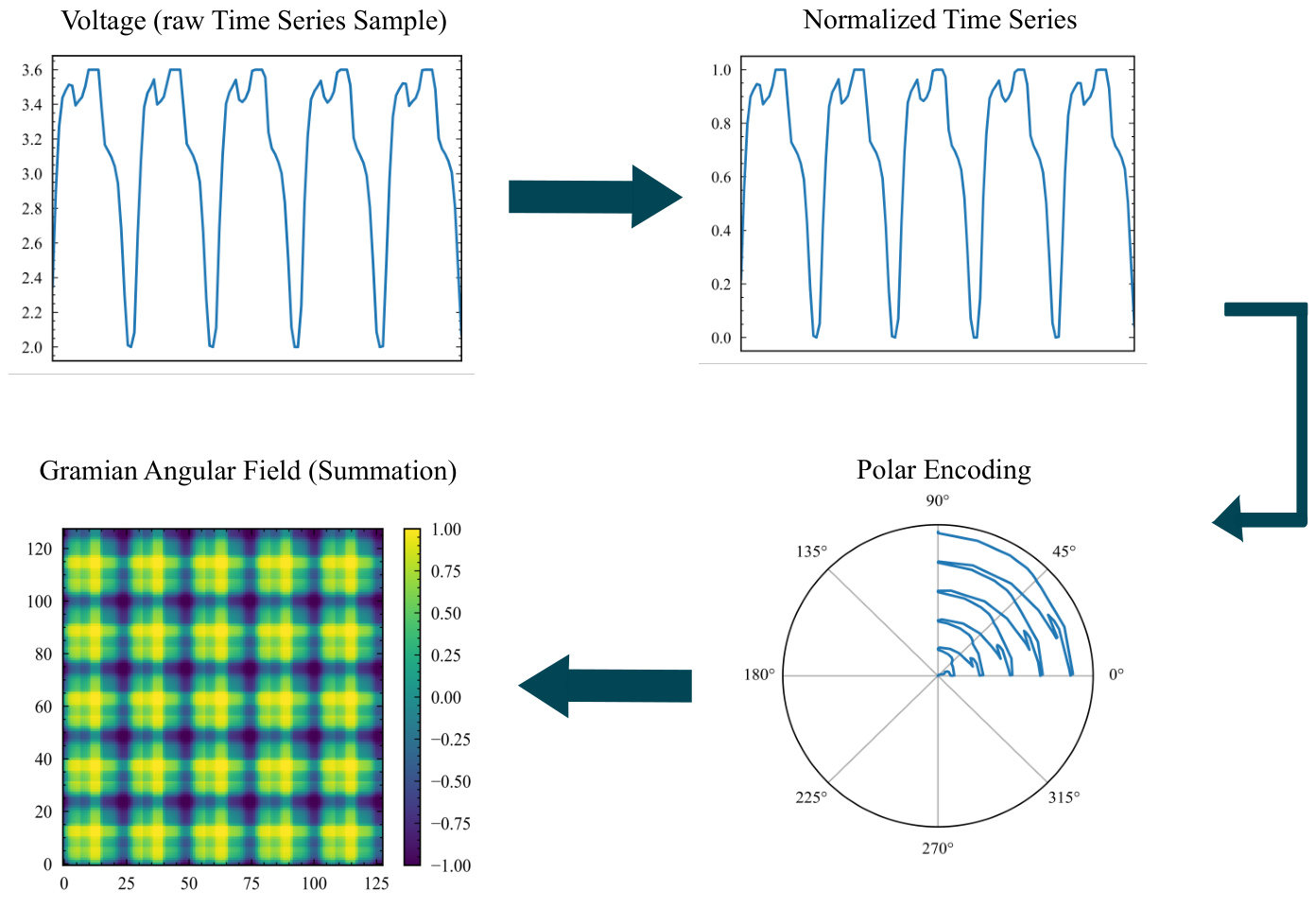
Two commonly used GAF representations are the Gramian Angular Summation Field (GASF) and Gramian Angular Difference Field (GADF). The GASF is obtained from the cosine of the sum of two angular coordinates, whereas the GADF is based on the sine of their difference. In this study, the GASF representation is used. For two time indices i and j, its elements are defined as
where denotes the element of the GASF matrix corresponding to time indices i and j, with . The variables and denote the angular coordinates defined in Equation (A2), while and are the corresponding normalised time-series values. The resulting GASF matrix has dimensions and encodes pairwise angular relationships between observations at different positions in the original sequence. The overall GAF encoding procedure is illustrated in Figure A1.
The GASF transformation is applied independently to each battery-data channel. The resulting channel-wise GASF matrices are stacked to form a tensor of dimensions , where C denotes the number of battery-data channels and H and W denote the height and width of each GAF representation, respectively. In the present work, , corresponding to voltage, current, temperature, capacity, and capacity fade. Each input sequence contains points, resulting in and therefore a GAF tensor of dimensions . These multichannel GAF tensors are subsequently used as inputs to the GAF GAN for synthetic battery-data generation.
References
- Ngoy, K.R.; Lukong, V.T.; Yoro, K.O.; Makambo, J.B.; Chukwuati, N.C.; Ibegbulam, C.; Eterigho-Ikelegbe, O.; Ukoba, K.; Jen, T.C. Lithium-ion batteries and the future of sustainable energy: A comprehensive review. Renew. Sustain. Energy Rev. 2025, 223, 115971. [Google Scholar] [CrossRef] [Scilit]
- Hu, X.; Xu, L.; Lin, X.; Pecht, M. Battery Lifetime Prognostics. Joule 2020, 4, 310–346. [Google Scholar] [CrossRef] [Scilit]
- Edge, J.S.; O’Kane, S.; Prosser, R.; Kirkaldy, N.D.; Patel, A.N.; Hales, A.; Ghosh, A.; Ai, W.; Chen, J.; Yang, J.; et al. Lithium ion battery degradation: What you need to know. Phys. Chem. Chem. Phys. 2021, 23, 8200–8221. [Google Scholar] [CrossRef] [Scilit] [PubMed]
- Maheshwari, A.; Paterakis, N.G.; Santarelli, M.; Gibescu, M. Optimizing the operation of energy storage using a non-linear lithium-ion battery degradation model. Appl. Energy 2020, 261, 114360. [Google Scholar] [CrossRef] [Scilit]
- Xu, W.; Mao, R.; Han, P.; Yuan, N.; Li, Y.; Guo, Y.; Zhang, H. A comprehensive review of lithium-ion battery remaining useful life prediction: Methodologies, datasets, performance metrics, and future perspectives. Meas. Sci. Technol. 2025, 36, 082001. [Google Scholar] [CrossRef] [Scilit]
- Yang, Y.; Xia, Q.; Yuan, L.; Zhao, P.; Xuan, L.; Liang, J. Lithium-ion battery state of health estimation using a hybrid model with multiple health indicators. J. Energy Storage 2026, 147, 120248. [Google Scholar] [CrossRef] [Scilit]
- Zhang, Y.; Li, Y.F. Prognostics and health management of Lithium-ion battery using deep learning methods: A review. Renew. Sustain. Energy Rev. 2022, 161, 112282. [Google Scholar] [CrossRef] [Scilit]
- Razavi-Far, R.; Farajzadeh-Zanjani, M.; Chakrabarti, S.; Saif, M. Data-driven prognostic techniques for estimation of the remaining useful life of lithium-ion batteries. In Proceedings of the 2016 IEEE International Conference on Prognostics and Health Management (ICPHM), Ottawa, ON, Canada; IEEE: New York, NY, USA, 2016; pp. 1–8. [Google Scholar] [CrossRef] [Scilit]
- Chen, D.; Zhang, W.; Zhang, C.; Sun, B.; Zhang, L.; Cong, X. Data-driven rapid lifetime prediction method for lithium-ion batteries under diverse fast charging protocols. J. Energy Storage 2023, 74, 109285. [Google Scholar] [CrossRef] [Scilit]
- Zhang, Y.; Zhao, M.; Xiong, R. Online data-driven battery life prediction and quick classification based on partial charging data within 10 min. J. Power Sources 2024, 594, 234007. [Google Scholar] [CrossRef] [Scilit]
- Xu, H.; Wu, L.; Xiong, S.; Li, W.; Garg, A.; Gao, L. An improved CNN-LSTM model-based state-of-health estimation approach for lithium-ion batteries. Energy 2023, 276, 127585. [Google Scholar] [CrossRef] [Scilit]
- Gu, X.; See, K.W.; Li, P.; Shan, K.; Wang, Y.; Zhao, L.; Lim, K.C.; Zhang, N. A novel state-of-health estimation for the lithium-ion battery using a convolutional neural network and transformer model. Energy 2023, 262, 125501. [Google Scholar] [CrossRef] [Scilit]
- Zraibi, B.; Okar, C.; Chaoui, H.; Mansouri, M. Remaining useful life assessment for lithium-ion batteries using CNN-LSTM-DNN hybrid method. IEEE Trans. Veh. Technol. 2021, 70, 4252–4261. [Google Scholar] [CrossRef] [Scilit]
- Yao, L.; Guo, M.; Fang, Z.; Chen, H.; Wang, P.; Xiao, Y. A review of data augmentation and evaluation for lithium-ion batteries from a temporal perspective. J. Energy Storage 2026, 165, 122337. [Google Scholar] [CrossRef] [Scilit]
- Zhao, G.; Zhang, C.; Duan, B.; Shang, Y.; Kang, Y.; Zhu, R. State-of-health estimation with anomalous aging indicator detection of lithium-ion batteries using regression generative adversarial network. IEEE Trans. Ind. Electron. 2023, 70, 2685–2695. [Google Scholar] [CrossRef] [Scilit]
- Gu, X.; See, K.; Liu, Y.; Arshad, B.; Zhao, L.; Wang, Y. A time-series Wasserstein GAN method for state-of-charge estimation of lithium-ion batteries. J. Power Sources 2023, 581, 233472. [Google Scholar] [CrossRef] [Scilit]
- Qiu, X.; Wang, S.; Chen, K. A conditional generative adversarial network-based synthetic data augmentation technique for battery state-of-charge estimation. Appl. Soft Comput. 2023, 142, 110281. [Google Scholar] [CrossRef] [Scilit]
- Hu, C.; Cheng, F.; Zhao, Y.; Guo, S.; Ma, L. State of charge estimation for lithium-ion batteries based on data augmentation with generative adversarial network. J. Energy Storage 2024, 80, 110004. [Google Scholar] [CrossRef] [Scilit]
- Sun, J.; Gu, A.; Kainz, J. A solution framework for the experimental data shortage problem of lithium-ion batteries: Generative adversarial network-based data augmentation for battery state estimation. J. Energy Chem. 2025, 103, 476–497. [Google Scholar] [CrossRef] [Scilit]
- Wang, Z.; Oates, T. Imaging time-series to improve classification and imputation. In Proceedings of the IJCAI’15: 24th International Conference on Artificial Intelligence, Buenos Aires, Argentina; AAAI Press: Washington, DC, USA, 2015; pp. 3939–3945. [Google Scholar]
- Das, O.; Sui, X.; Sanfilippo, F.; Rudra, S. Battery Time-Series Data Augmentation Using a GAF-Based Generative Framework. In Proceedings of the IEEE EUROCON 2025-21st International Conference on Smart Technologies, Gdynia, Poland; IEEE: New York, NY, USA, 2025; pp. 1–6. [Google Scholar] [CrossRef] [Scilit]
- Liu, X.; Zhou, L.; Tian, J.; Wu, L.; Wei, Z.; Hasanien, H.M.; Wang, P. Battery SOH enhanced solution: Voltage reconstruction and image recognition response to loss of data scenarios. J. Energy Chem. 2026, 112, 155–169. [Google Scholar] [CrossRef] [Scilit]
- Xiang, H.; Wang, Y.; Soo, Y.Y.; Xiong, X.; Chen, Z. Predicting automotive battery degradation trajectories using transformer with variational auto-encoder based data augmentation. IEEE Trans. Veh. Technol. 2025, 74, 10368–10379. [Google Scholar] [CrossRef] [Scilit]
- Yang, Z.; Pan, Y.; Liu, W.; Meng, J.; Song, Z. Enhanced fault detection in lithium-ion battery energy storage systems via transfer learning-based conditional GAN under limited data. J. Power Sources 2025, 645, 237192. [Google Scholar] [CrossRef] [Scilit]
- Goodfellow, I.J.; Pouget-Abadie, J.; Mirza, M.; Xu, B.; Warde-Farley, D.; Ozair, S.; Courville, A.; Bengio, Y. Generative Adversarial Nets. In Proceedings of the Advances in Neural Information Processing Systems, Montreal, QC, Canada; Ghahramani, Z., Welling, M., Cortes, C., Lawrence, N., Weinberger, K., Eds.; Curran Associates, Inc.: Red Hook, NY, USA, 2014; Volume 27. [Google Scholar]
- Zheng, M.; Li, T.; Zhu, R.; Tang, Y.; Tang, M.; Lin, L.; Ma, Z. Conditional Wasserstein generative adversarial network-gradient penalty-based approach to alleviating imbalanced data classification. Inf. Sci. 2020, 512, 1009–1023. [Google Scholar] [CrossRef] [Scilit]
- Mirza, M.; Osindero, S. Conditional Generative Adversarial Nets. arXiv 2014. [Google Scholar] [CrossRef] [Scilit]
- Arjovsky, M.; Chintala, S.; Bottou, L. Wasserstein Generative Adversarial Networks. In Proceedings of the 34th International Conference on Machine Learning, PMLR, Sydney, Australia; Precup, D., Teh, Y.W., Eds.; Proceedings of Machine Learning Research: Cambridge, MA, USA, 2017; Volume 70, pp. 214–223. [Google Scholar]
- Gulrajani, I.; Ahmed, F.; Arjovsky, M.; Dumoulin, V.; Courville, A. Improved Training of Wasserstein GANs. In Proceedings of the Advances in Neural Information Processing Systems, Long Beach, CA, USA; Guyon, I., Luxburg, U.V., Bengio, S., Wallach, H., Fergus, R., Vishwanathan, S., Garnett, R., Eds.; Curran Associates, Inc.: Red Hook, NY, USA, 2017; Volume 30. [Google Scholar]
- de Vries, H.; Strub, F.; Mary, J.; Larochelle, H.; Pietquin, O.; Courville, A. Modulating early visual processing by language. In Proceedings of the Advances in Neural Information Processing Systems, Long Beach, CA, USA; Guyon, I., Luxburg, U.V., Bengio, S., Wallach, H., Fergus, R., Vishwanathan, S., Garnett, R., Eds.; Curran Associates, Inc.: Red Hook, NY, USA, 2017; Volume 30. [Google Scholar]
- Miyato, T.; Koyama, M. cGANs with Projection Discriminator. arXiv 2018. [Google Scholar] [CrossRef] [Scilit]
- Wu, Y.; He, K. Group Normalization. In Proceedings of the European Conference on Computer Vision (ECCV), Munich, Germany; Computer Vision Foundation: New York, NY, USA, 2018. [Google Scholar]
- Miyato, T.; Kataoka, T.; Koyama, M.; Yoshida, Y. Spectral Normalization for Generative Adversarial Networks. arXiv 2018. [Google Scholar] [CrossRef] [Scilit]
- Yoon, J.; Jarrett, D.; van der Schaar, M. Time-series Generative Adversarial Networks. In Proceedings of the Advances in Neural Information Processing Systems, Vancouver, BC, Canada; Wallach, H., Larochelle, H., Beygelzimer, A., D’Alché-Buc, F., Fox, E., Garnett, R., Eds.; Curran Associates, Inc.: Red Hook, NY, USA, 2019; Volume 32. [Google Scholar]
- Heusel, M.; Ramsauer, H.; Unterthiner, T.; Nessler, B.; Hochreiter, S. GANs Trained by a Two Time-Scale Update Rule Converge to a Local Nash Equilibrium. In Proceedings of the Advances in Neural Information Processing Systems, Long Beach, CA, USA; Guyon, I., Luxburg, U.V., Bengio, S., Wallach, H., Fergus, R., Vishwanathan, S., Garnett, R., Eds.; Curran Associates, Inc.: Red Hook, NY, USA, 2017; Volume 30. [Google Scholar]
- Binkowski, M.; Sutherland, D.J.; Arbel, M.; Gretton, A. Demystifying MMD GANs. arXiv 2018. [Google Scholar] [CrossRef] [Scilit]
- Sajjadi, M.S.M.; Bachem, O.; Lucic, M.; Bousquet, O.; Gelly, S. Assessing Generative Models via Precision and Recall. In Proceedings of the Advances in Neural Information Processing Systems, Montreal, QC, Canada; Bengio, S., Wallach, H., Larochelle, H., Grauman, K., Cesa-Bianchi, N., Garnett, R., Eds.; Curran Associates, Inc.: Red Hook, NY, USA, 2018; Volume 31. [Google Scholar]
- Kynkäänniemi, T.; Karras, T.; Laine, S.; Lehtinen, J.; Aila, T. Improved Precision and Recall Metric for Assessing Generative Models. In Proceedings of the Advances in Neural Information Processing Systems, Vancouver, BC, Canada; Wallach, H., Larochelle, H., Beygelzimer, A., D’Alché-Buc, F., Fox, E., Garnett, R., Eds.; Curran Associates, Inc.: Red Hook, NY, USA, 2019; Volume 32. [Google Scholar]
- Seol, S.; Yoon, J.; Lee, J.; Kim, B. Metrics for evaluating synthetic time-series data of battery. Appl. Sci. 2024, 14, 6088. [Google Scholar] [CrossRef] [Scilit]
- Lucic, M.; Kurach, K.; Michalski, M.; Gelly, S.; Bousquet, O. Are GANs Created Equal? A Large-Scale Study. In Proceedings of the Advances in Neural Information Processing Systems, Montreal, QC, Canada; Bengio, S., Wallach, H., Larochelle, H., Grauman, K., Cesa-Bianchi, N., Garnett, R., Eds.; Curran Associates, Inc.: Red Hook, NY, USA, 2018; Volume 31. [Google Scholar]
- Borji, A. Pros and cons of GAN evaluation measures: New developments. Comput. Vis. Image Underst. 2022, 215, 103329. [Google Scholar] [CrossRef] [Scilit]
- Tarvainen, A.; Valpola, H. Mean teachers are better role models: Weight-averaged consistency targets improve semi-supervised deep learning results. In Proceedings of the Advances in Neural Information Processing Systems, Long Beach, CA, USA; Guyon, I., Luxburg, U.V., Bengio, S., Wallach, H., Fergus, R., Vishwanathan, S., Garnett, R., Eds.; Curran Associates, Inc.: Red Hook, NY, USA, 2017; Volume 30. [Google Scholar]
- Severson, K.A.; Attia, P.M.; Jin, N.; Perkins, N.; Jiang, B.; Yang, Z.; Chen, M.H.; Aykol, M.; Herring, P.K.; Fraggedakis, D.; et al. Data-driven prediction of battery cycle life before capacity degradation. Nat. Energy 2019, 4, 383–391. [Google Scholar] [CrossRef] [Scilit]
- Attia, P.M.; Grover, A.; Jin, N.; Severson, K.A.; Markov, T.M.; Liao, Y.H.; Chen, M.H.; Cheong, B.; Perkins, N.; Yang, Z.; et al. Closed-loop optimization of fast-charging protocols for batteries with machine learning. Nature 2020, 578, 397–402. [Google Scholar] [CrossRef] [Scilit] [PubMed]
- Garapati, V.K.; Huld, F.; Lee, H.; Lamb, J.J. New algorithm for battery knee-onset identification and early prediction of end of life. Mach. Learn. Eng. 2026, 2, 015004. [Google Scholar] [CrossRef] [Scilit]
- Keogh, E.; Chakrabarti, K.; Pazzani, M.; Mehrotra, S. Dimensionality Reduction for Fast Similarity Search in Large Time Series Databases. Knowl. Inf. Syst. 2001, 3, 263–286. [Google Scholar] [CrossRef] [Scilit]
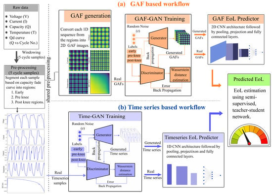
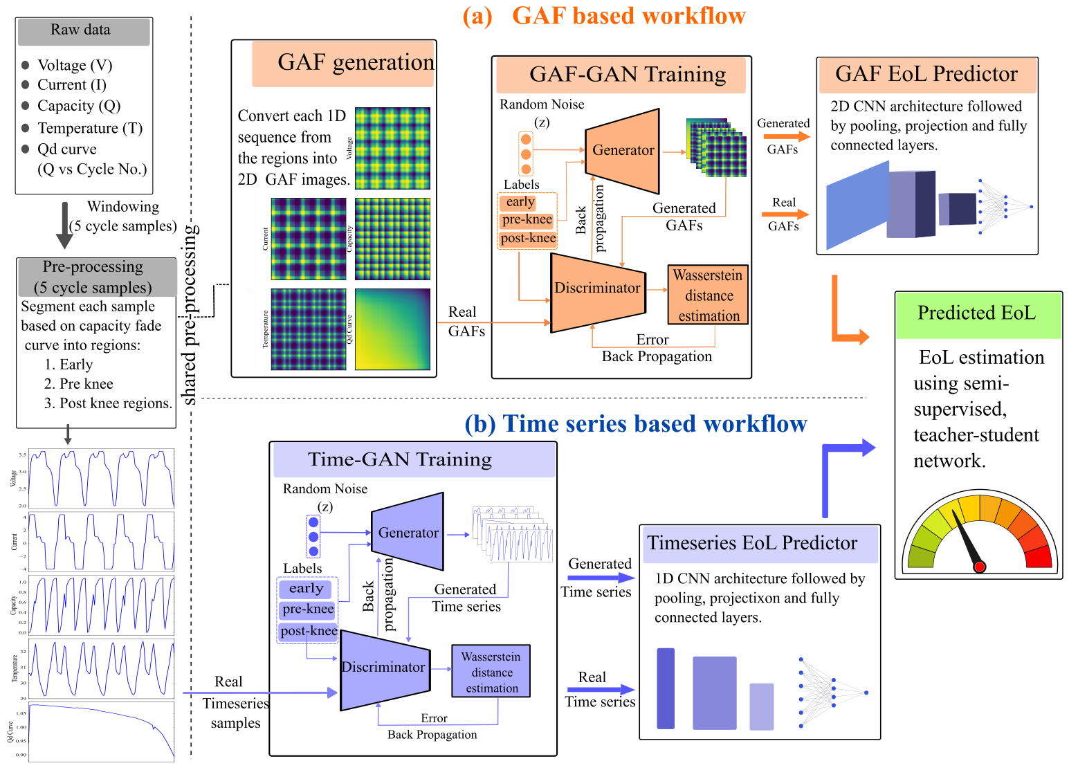
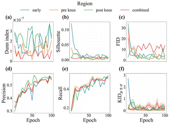
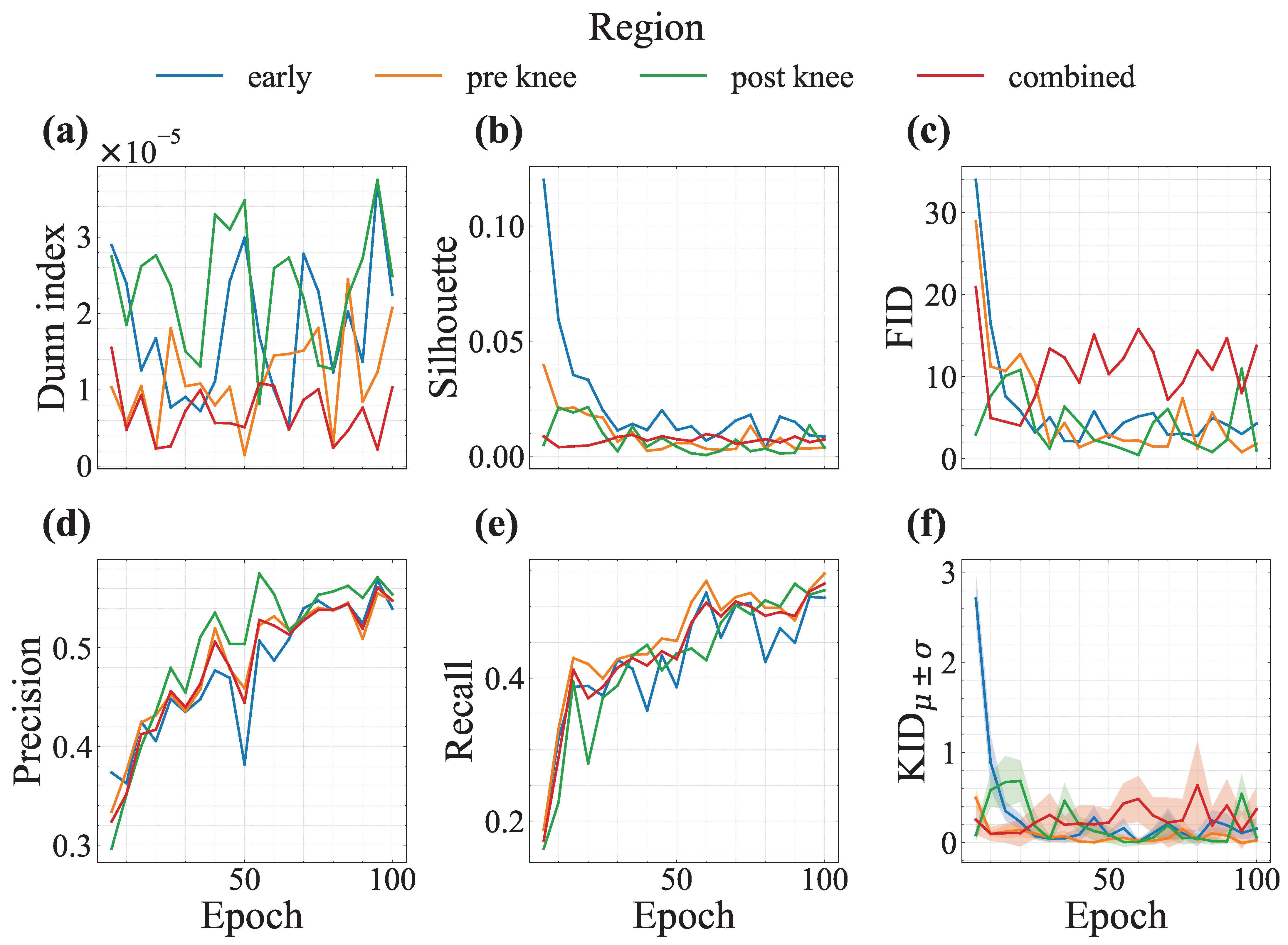
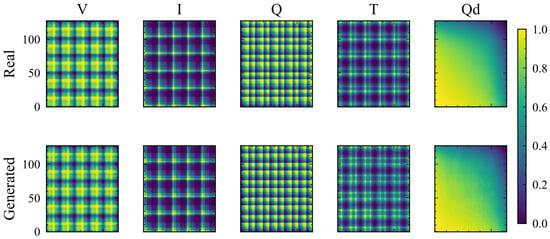
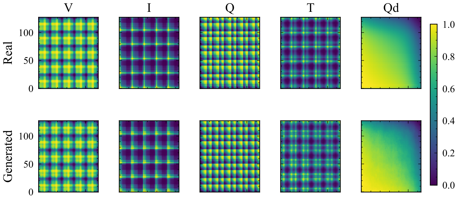
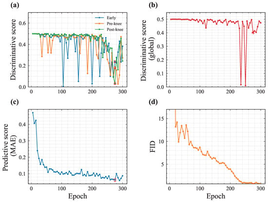
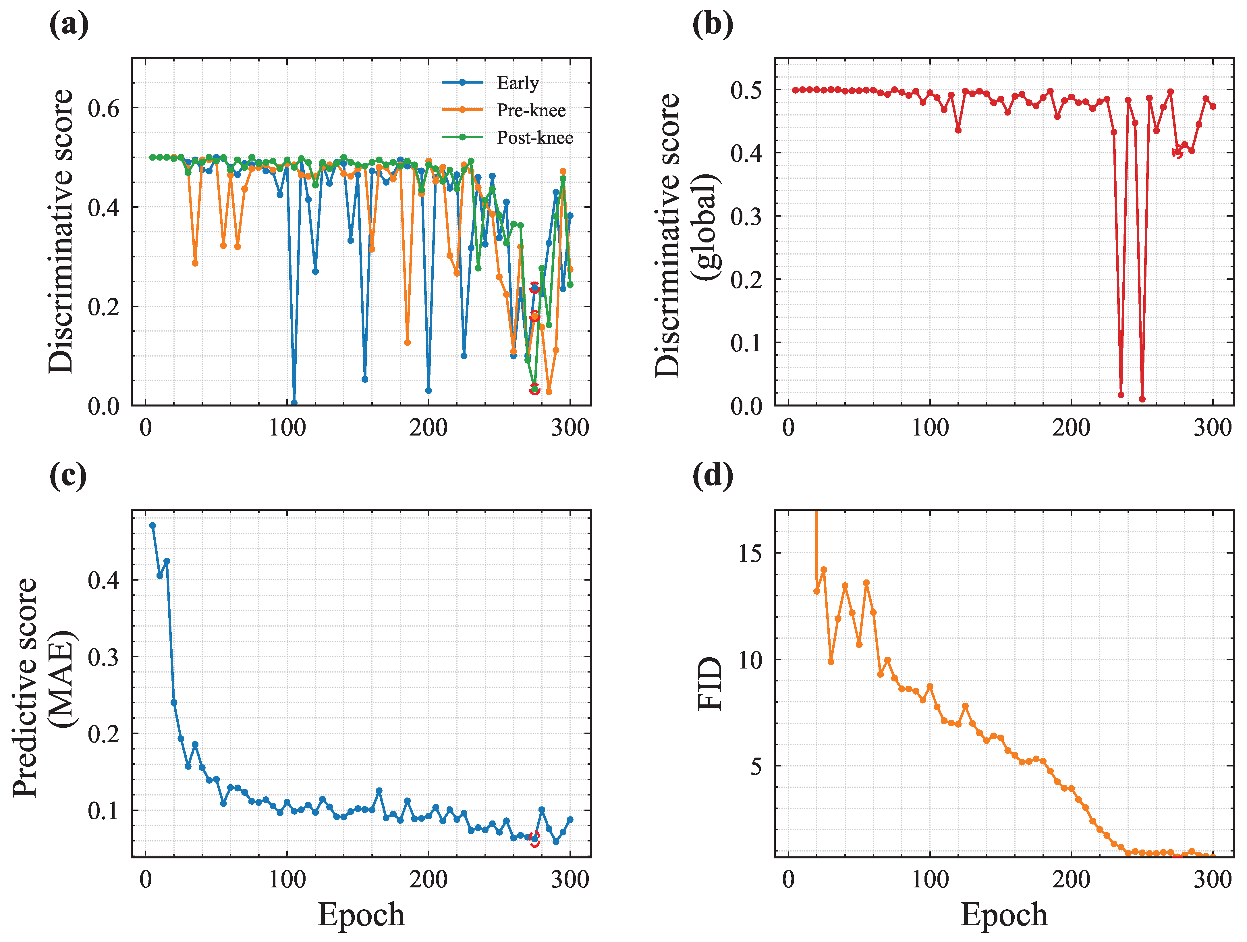
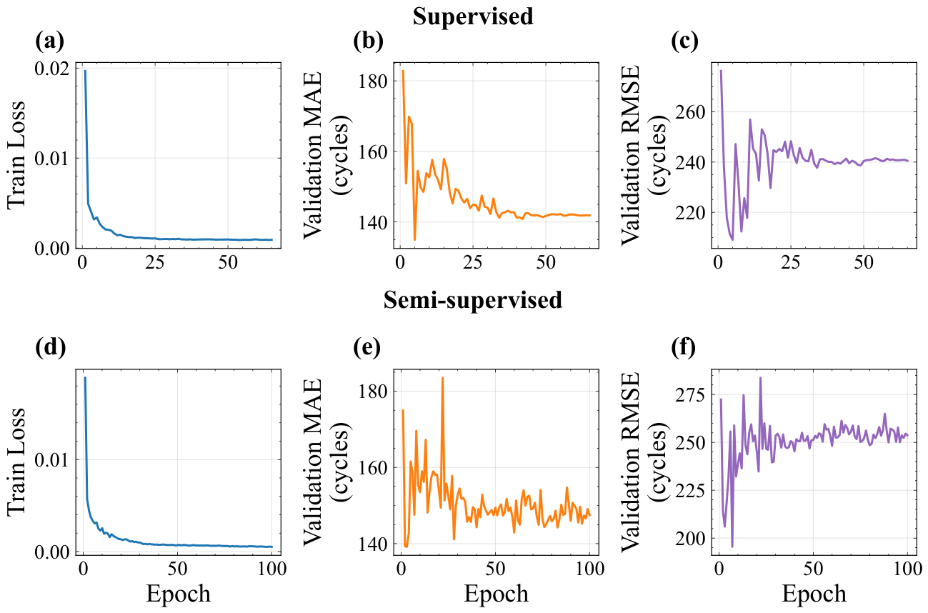
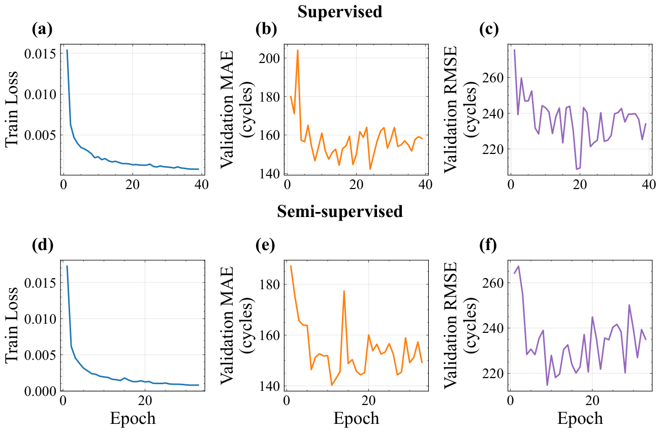
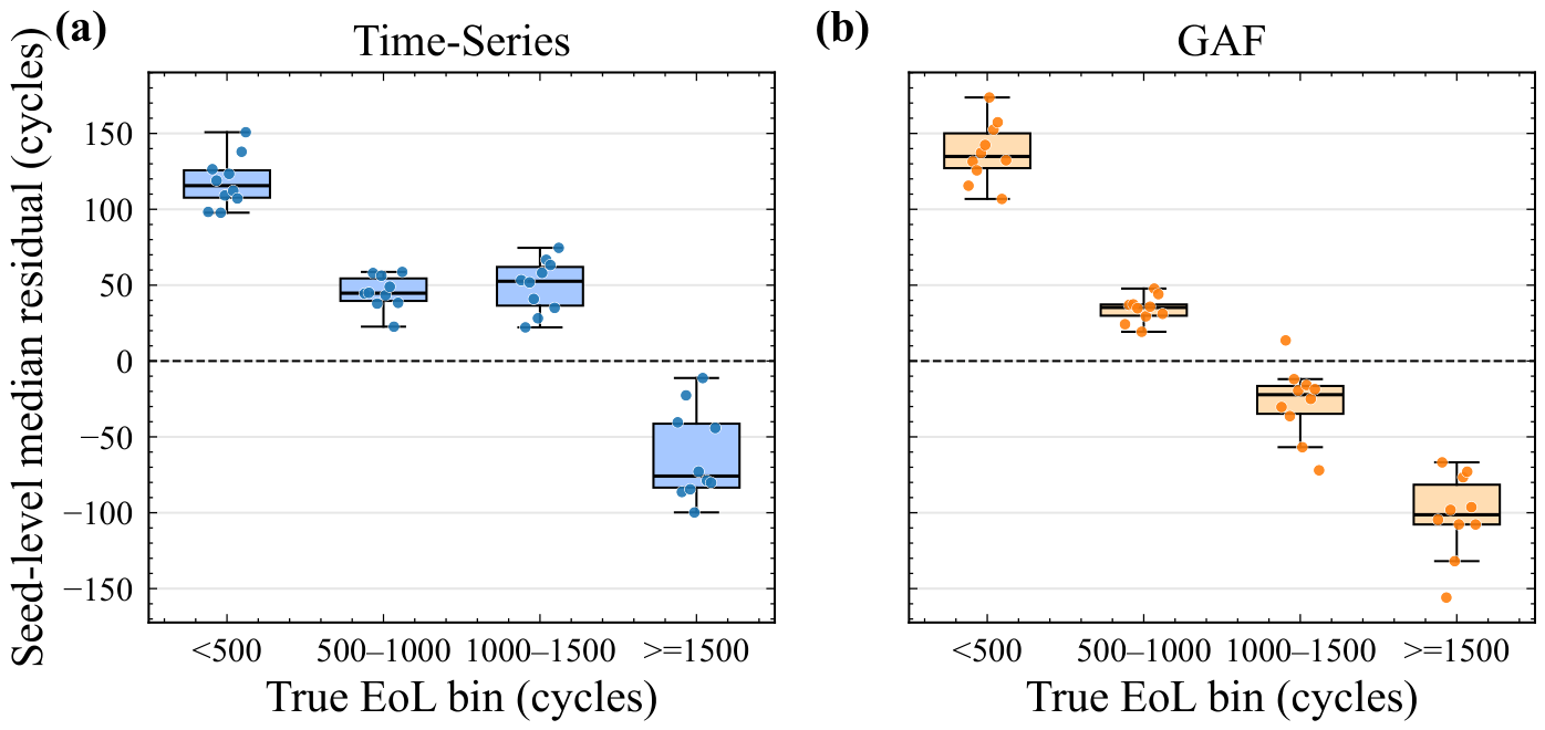

Disclaimer/Publisher’s Note: The statements, opinions and data contained in all publications are solely those of the individual author(s) and contributor(s) and not of MDPI and/or the editor(s). MDPI and/or the editor(s) disclaim responsibility for any injury to people or property resulting from any ideas, methods, instructions or products referred to in the content. |
© 2026 by the authors. Licensee MDPI, Basel, Switzerland. This article is an open access article distributed under the terms and conditions of the Creative Commons Attribution (CC BY) license.