Online Health Estimation of Batteries with Moderate to High Degradation Utilizing LSTM-Ensembled Learning Framework from Consecutive CC Charging Segments

Abstract

Accurate online state of health (SoH) estimation, especially for highly degraded second-life batteries (SLBs), is critical for the safe and efficient operation of any Battery Management System (BMS). However, existing data-driven estimation methods typically rely on complete charge/discharge cycles or assume a fixed starting state of charge (SoC) and fixed voltage windows. These assumptions are highly restrictive and rarely align with the random, partial charging behaviors of real-world electric vehicle (EV) operations and Battery Energy Storage System (BESS) applications. To overcome this limitation, this paper presents the following framework: an online SoH estimation approach utilizing long short-term-memory (LSTM)-ensembled learning using consecutive constant current (CC) charging segments. Instead of relying on a rigid voltage window, the presented method utilizes nested, expanding slices of highly flexible CC charging intervals to capture sequential degradation dynamics. Furthermore, this study maps suggestive ranges of optimal voltage intervals that dynamically adapt to different battery health conditions, ensuring high estimation accuracy despite the type of degradation. The framework is validated using four commercially available lithium-ion batteries (LIBs), with a moderate to low SoH down to ~40%. To ensure practical viability, the hybrid deep neural network (DNN) and LSTM architecture has been highly optimized, requiring only 474 trainable parameters. The framework has been evaluated utilizing multiple performance matrices, showing minimal discrepancy with excellent correlation to the true SoH throughout the lifespan of the testing cell.

1. Introduction

The rapid proliferation of electric vehicles (EVs) and grid-scale energy storage systems has solidified lithium-ion batteries (LIBs) as the cornerstone of modern energy transition [1,2]. To ensure the safe, efficient, and reliable operation of these battery packs, a robust Battery Management System (BMS) is essential. One of the most critical functions of the BMS is the accurate estimation of the state of health (SoH), which quantifies the degradation of the battery’s maximum capacity over time [3,4]. Accurate SoH estimation prevents catastrophic failures, mitigates range anxiety for EV drivers, and optimizes charging strategies to extend battery life [5].

In recent years, data-driven SoH estimation methods, particularly leveraging Artificial Intelligence (AI), have shown immense promise due to their ability to model complex, non-linear degradation patterns without requiring intricate electrochemical equations [6,7]. However, most of the existing empirical studies rely on highly restrictive assumptions. Specifically, these models often require complete charge and discharge cycles, or they rely on partial charging curves with a rigidly fixed initial state of charge (SoC) and a fixed voltage window [8,9]. In real-world EV operation scenarios, charging behavior is inherently stochastic; drivers plug in their vehicles at random SoC levels and unplug them before reaching a full charge [10]. Consequently, models trained on fixed voltage windows and fixed starting points may fail or suffer severe accuracy drops when applied to empirical, real-world data where the anticipated starting voltage is unavailable.

Furthermore, traditional fixed-window approaches often overlook the underlying electrochemical degradation mechanisms that alter the battery’s behavior across different voltage ranges. Battery aging is primarily driven by loss of lithium inventory (LLI) and loss of active material (LAM) [11]. As the battery ages and transitions towards its second life, LLI typically causes the electrode utilization windows to shift, while LAM reduces the total capacity. These internal mechanisms dictate that not all voltage ranges degrade at the same rate or exhibit the same sensitivity to aging [12]. As a result, the open-circuit voltage (OCV) characteristics and the corresponding constant current (CC) charging durations shift dynamically over the battery’s lifespan [13]. Ignoring these shifting effects and failing to capture the sequential correlation of consecutive voltages during the CC charging phase, resulting in the loss of critical degradation memory, may lead to suboptimal SoH predictions [14,15].

To capture these complex temporal dependencies, the recent literature has increasingly turned to deep sequential architectures, including heavy networks, transformers, and hybrid regressor ensembles operating on CC charging profiles. Primarily, many models rigidly rely on full charge cycles [16] or fixed-length, narrow SoC windows, failing to accommodate the partial and interrupted charging sessions typical of real-world operations [17,18,19]. While single-feature regressors and incremental capacity analysis (ICA) offer algorithmic simplicity, they inherently sacrifice robustness under variable conditions and remain highly sensitive to practical sensor noise [20,21]. To address variable partial charging, recent studies have explored stochastic segment selection and raw curve processing. However, these methods—along with shallow regressors—lack structured inter-cycle aggregation mechanisms, leaving cycle-to-cycle prediction variance unaddressed [15,22,23]. Furthermore, efforts to capture complex spatiotemporal degradation often rely on excessively heavy architectures, such as graph neural networks or multi-model stacking ensembles, which are computationally prohibitive for kilobyte-scale BMS microcontrollers [19,24].

To address these critical gaps, this paper presents the following framework: utilizing LSTM-ensembled learning using partial consecutive CC charging segments to estimate SoH in real time. This approach abandons the restrictive fixed-window assumption in favor of nested, expanding slices of highly flexible consecutive CC charging intervals. By analyzing sequential voltage data, the model implicitly captures the localized impacts of LLI and LAM without requiring a rigid starting point. Furthermore, we identified and mapped a suggestive range of optimal voltage intervals that adapt to different health conditions, ensuring the BMS utilizes the most highly correlated data for estimation at any stage of the batteries’ useful life, mostly for second-life batteries (SLB). Finally, the presented hybrid architecture is explicitly optimized for low-cost edge deployment. The main contributions of the work presented in this paper are summarized as follows:

• Elimination of Fixed-Window Constraints: We introduce a nested, expanding sequence of CC charging intervals of variable lengths that enables accurate SoH estimation from fragmented, partial CC charging data with variable starting points.
• Degradation-Aware Voltage Mapping: We analyze the varying impacts of aging across different voltage ranges and provide a suggestive mapping of optimal estimation intervals tailored to shifting health conditions.
• Ultra-Lightweight Edge Framework: We design a highly optimized, parameter-efficient model (requiring only 474 parameters and <0.03 MB of memory) that is fully deployable to low-cost edge devices, ensuring seamless integration into low-cost BMS microcontrollers.

The remainder of this paper is organized as follows: Section 2 details the overview of the framework, including the data acquisition and model preparation steps. Section 3 presents the performance results and discussions on the validation of edge-deployment feasibility. Finally, Section 4 draws conclusions and outlines future work regarding temperature and C-rate scalability.

2. Overview of the Framework

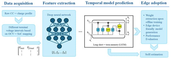
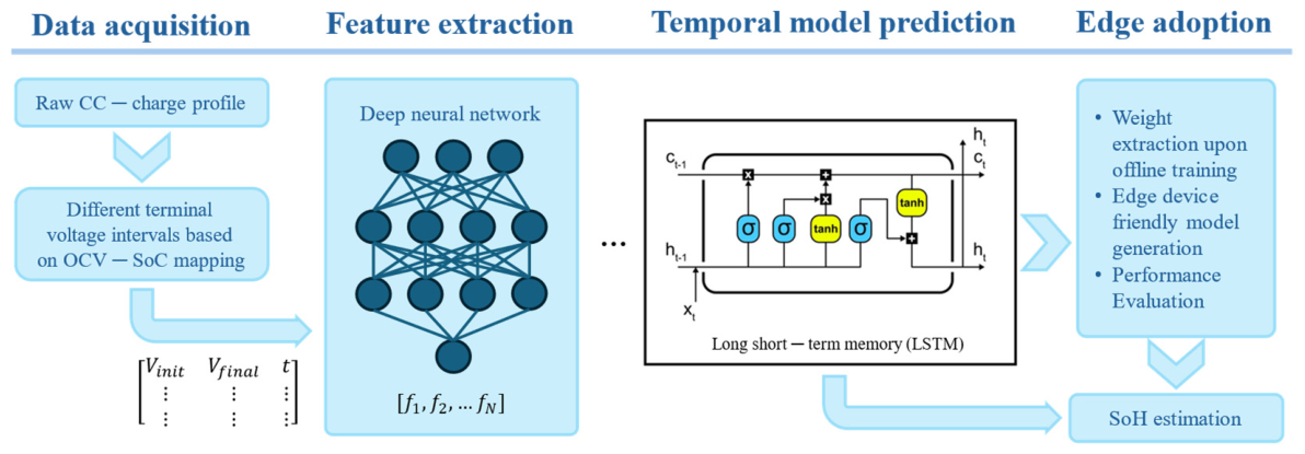
In this study, a framework has been developed that enables BMSs to track the SoH using the regular voltage measurements of the LIBs without the need for specialized electronic components that are required for obtaining complex characteristics such as electrochemical impedance spectroscopy (EIS) or the hybrid pulse power characteristics (HPPC). In the presented approach, the consecutive voltage measurements from the CC-charging phase over variable initial conditions and voltage intervals are used to train a three-layer deep neural network (DNN), which generates a sequence of several SoH estimations from different voltage intervals of the CC-charging phase. The length of the sequence depends on the end voltage requirement, or the constant voltage (CV) based charging condition. The sequence is then fed through an LSTM model for extracting the temporal dependencies among different segments of the voltage profile and finally a single dense layer for SoH estimation. As the sequence will be strictly chronological from the beginning of the CC-charging to the end, the unidirectional LSTM over its bidirectional variation has been chosen to reduce model complexity and minimize the parameter counts [25]. The overall flow of the approach, from data acquisition to edge adoption, has been shown in Figure 1.

Figure 1. Methodological flowchart of the presented framework.

2.1. Data Acquisition and Preprocessing

For the training and validation purposes of the presented ensemble learning machine, four commercial cylindrical cells by LG have been cycled using the Squidstat cycler (Admiral Instruments, Tempe, AZ, USA) [26]. The characteristics of the selected cell and the description of the experimental setup have been listed in Table 1. For this specific architecture, a controlled ambient temperature of 15 °C has been achieved using a TestEquity thermal chamber (North Richland Hills, TX, USA) [27], and a 1C rate for both constant current-constant voltage (CCCV) charging and CC discharging of the full operating voltage range has been considered. This controlled experiment allowed the presented model to be dependent only on the voltage profile for SoH estimation, although the model can also be modified to utilize both the temperature and the charging C-rate, which is out of the scope for this investigation.

Table 1. Characteristics of INR18650MJ1 and the experimental design [28].

Characteristics	Values
Commercial name	INR18650MJ1
Type	NMC Cylindrical Cell
Nominal voltage	3.635 V
Capacity	3.5 Ah
Experimental C-rate	1 C (3.4 A) [Both charge and discharge]
Experiment temperature	15 °C (controlled)
Rest period between charge and discharge	30 min
Full cycle count	174 for each cell (~70% capacity fading)
Number of cells used	3 for training and validation; 1 for testing

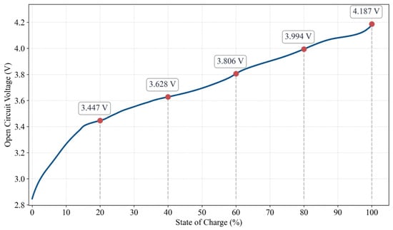
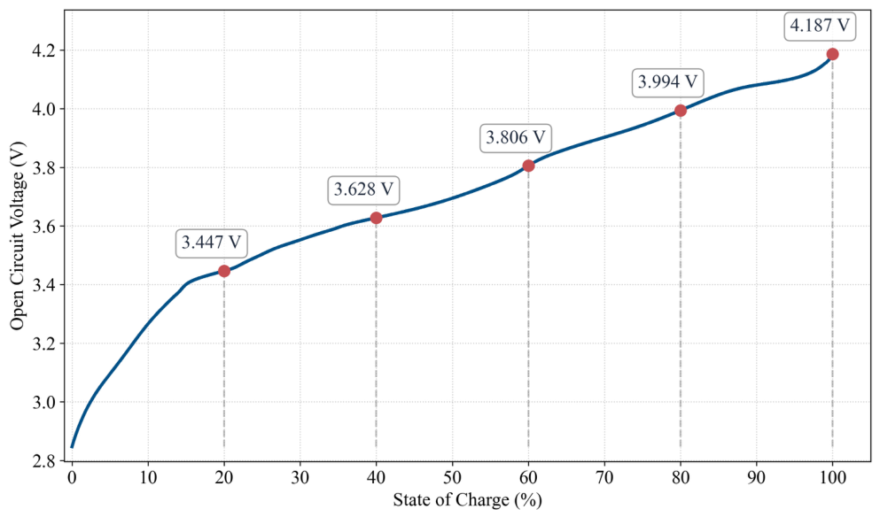
Now, unlike laboratory environments, where LIBs are subjected to complete 0–100% CC-CV cycles, empirical studies demonstrate that real-world charging is highly stochastic [29]. Due to range anxiety and the tapering limits of fast chargers, charging events predominantly manifest as fragmented in nature, typically initiating between 40 and 60% SoC and terminating near 80% SoC [30]. Consequently, traditional SoH estimation methods that rely on fixed starting voltages or complete CC profiles are rendered largely ineffective in practical BMS deployments [31]. Considering all these circumstances, in this study, the OCV characteristics of the battery have been adopted to obtain corresponding voltages at five standard SoC intervals that cover most of the charging scenario for any typical LIB application: 20%, 40%, 60%, 80%, and 100%. For the OCV characteristics acquisition, the testing cell has been discharged at a C/72 rate, which is the cutoff limit of the CV mode charging and low enough to neglect the polarization effect of the cell terminal voltage [28]. Figure 2 shows the mapping of OCVs at different SoC intervals.

Figure 2. OCV characteristics of INR18650MJ1 and corresponding OCVs at 5 SoC intervals.

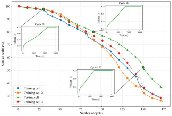
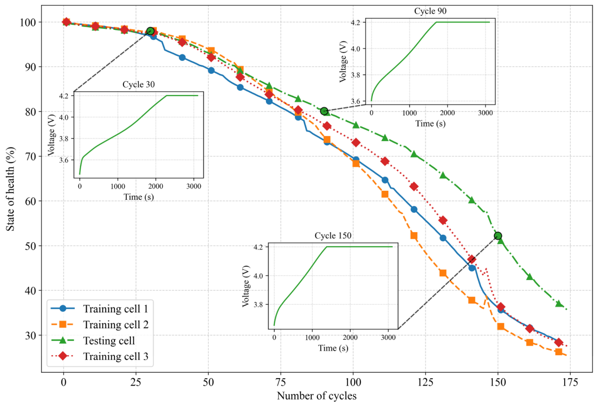
For the presented model, three inputs have been considered: the initial voltage, $V_{init}$, the final voltage, $V_{final}$, and the time interval to reach from that initial voltage to the final voltage, $t$. With the five selected OCVs and the typical charging patterns, we considered nine sets of input combinations for each CC-charging phase: 20–40%, 20–60%, 20–80%, 20–100%, 40–60%, 40–80%, 40–100%, 60–80%, and 60–100%. Note that the SoC intervals shown are used solely as reference points for identifying the corresponding voltage values, not as actual SoC values during CC charging. The true SoCs at 1C charging rate would be significantly lower and were not used as model inputs. All the cells have been cycled 174 times and the average capacity fading achieved for all the cells is roughly 70% considering the initial capacity as the beginning of life (BOL) capacity. Figure 3 shows how the SoH changes throughout the cycles. An important observation from the figure, as the cell loses its capacity, the CC-charging phase period shrinks, which has been illustrated carefully with the real-time voltage profile at three different cycles with identical X-axis range.

Figure 3. SoH evolution over the number of cycles for all the cells used in this study, with the charging profile at different cycles over the lifetime of the testing cell.

To understand how the inputs will look like for a certain CC-charging phase, let us consider a scenario when a cell has been charged from 20% to 80% SoC. In that case, if we consider the interval to be 20%, three samples will be prepared that will move sequentially into the presented model for SoH estimation purpose; from 20–40%, 20–60% and 20–80%. For each sample, there will be a fixed $V_{init}$, the corresponding $V_{final}$ for the intermediate SoC after certain intervals and the time required for the cell to reach that voltage. Note that, in this study, 1C has been considered, so the time required for consecutive ranges looked almost linear with a uniform SoC interval. With the same condition, if the charging begins from a higher SoC value, let us consider 40%, then the number of samples will be two instead of three, and the model will automatically consider one less DNN stage for SoH estimation, resulting in less computational burden on the system. Among four cells that have been cycled, three have been considered for training and validation purposes, and one has been considered exclusively for testing purposes to obtain unbiased performance of the presented approach.

2.2. LSTM-Ensembled Model Architecture

The presented model is a compact hybrid architecture comprising three sequentially coupled modules: a voltage range-distributed Base DNN for interval-wise feature compression, a single-layer LSTM for the extraction of the temporal dependencies, and a dense prediction head for continuous SoH regression. The complete layer specification is summarized in Table 2. The total trainable parameter count is 474, making the model amenable to deployment on resource-constrained BMS embedded processors without quantization. The input tensor carries shape (1, X, 3), representing a single-sample batch of X consecutive CC-charging intervals (X ranging from 2 to 4 depending on the starting SoC of the partial charge), each described by three health-sensitive features extracted from the voltage–time profile.

Table 2. Presented ensembled LSTM architecture considering X consecutive measurements.

Component	Layer Type	Input Shape	Output Shape	Parameters	Activation
Input	Sequential Raw Data	[1, X *, 3]	[1, X, 3]	0	None
Base DNN	Dense (Linear 1)	[X, 3]	[X, 8]	32	LeakyReLU
	Dense (Linear 2)	[X, 8]	[X, 8]	72	LeakyReLU
	Dense (Linear 3)	[X, 8]	[X, 1]	9	None
Temporal Tracking	LSTM (1 Layer)	[X, 1]	[X, 8]	352	Tanh/Sigmoid
Prediction Head	Dense (Output)	[1, 8]	[1, 1]	9	Sigmoid

* X is the number of consecutive measurements after each interval, comprising a common initial voltage, the voltage after a specific interval, and the time of the interval.

2.2.1. Base DNN

The Base DNN is applied identically and independently to each of the S time steps via a time-distributed wrapper, consistent with the architecture introduced by Chollet [32]. The module consists of three fully connected layers. For a single time step $\mathrm{s}\in \{1,\hspace{0.17em}\dots ,\hspace{0.17em}S\}$, the forward pass proceeds as described below.

The first layer projects the feature vector into an eight-dimensional hidden space:

$$h_{s,1}=\mathrm{L}\mathrm{e}\mathrm{a}\mathrm{k}\mathrm{y}\mathrm{R}\mathrm{e}\mathrm{L}\mathrm{U}\left(W_1{x}_s\hspace{0.17em}+\hspace{0.17em}{b}_1\right)$$

(1)

where $x_s\in {\mathbb{R}}^{\mathbb{3}}$ is the feature vector at interval s, $W_1\in {\mathbb{R}}^{\mathbb{8}\times \mathbb{3}}$, and $b_1\in {\mathbb{R}}^{\mathbb{8}}$. This layer contributes 3 × 8 + 8 = 32 parameters. The Leaky Rectified Linear Unit (LeakyReLU) activation is defined as follows [33]:

$$\mathrm{L}\mathrm{e}\mathrm{a}\mathrm{k}\mathrm{y}\mathrm{R}\mathrm{e}\mathrm{L}\mathrm{U}\left(z\right)=\left\{\begin{array}{c}z,\hspace{0.17em}if\hspace{0.17em}z\ge 0\\ \mathrm{\alpha }z,\hspace{0.17em}Otherwise\end{array}\right.$$

(2)

where $\mathrm{\alpha }\hspace{0.17em}=\hspace{0.17em}0.01$ is the negative-slope coefficient. The second hidden layer maintains the eight-dimensional representation:

$$h_{s,2}=\mathrm{L}\mathrm{e}\mathrm{a}\mathrm{k}\mathrm{y}\mathrm{R}\mathrm{e}\mathrm{L}\mathrm{U}\left(W_2{h}_{s,1}\hspace{0.17em}+\hspace{0.17em}{b}_2\right)$$

(3)

where $W_2\in {\mathbb{R}}^{\mathbb{8}\times \mathbb{8}}$ and $b_2\in {\mathbb{R}}^{\mathbb{8}}$, yielding 8 × 8 + 8 = 72 parameters. The third layer compresses the representation to a scalar encoding:

$$z_s=W_3{h}_{s,2}+b_3$$

(4)

where $W_3\in {\mathbb{R}}^{\mathbb{1}\times \mathbb{8}}$ and $b_3\in {\mathbb{R}}^{\mathbb{1}}$, contributing 8 + 1 = 9 parameters. No activation is applied at this layer, preserving linearity of the scalar projection. The resulting time-distributed output $\mathrm{Z}=\hspace{0.17em}{z}_1,\hspace{0.17em}\dots \hspace{0.17em},\hspace{0.17em}{z}_s\in {\mathbb{R}}^{\mathbb{s}\times \mathbb{1}}$ constitutes the compressed interval-level representation fed to the LSTM layer.

2.2.2. LSTM Layer

A single-layer LSTM network [34] processes the compressed sequence $\mathrm{Z}\in {\mathbb{R}}^{\mathbb{4}\times \mathbb{1}}$ to extract the temporal dependencies across consecutive voltage intervals. For each time step $\mathrm{s}$, the LSTM computes:

$$i_s=\mathrm{\sigma }\left(W_{ii}{z}_s+W_{hi}{h}_{s-1}+b_i\right)$$

(5)

$$f_s=\mathrm{\sigma }\left(W_{if}{z}_s\hspace{0.17em}+\hspace{0.17em}{W}_{hf}{h}_{s-1}\hspace{0.17em}+\hspace{0.17em}{b}_f\right)$$

(6)

$$g_s=\mathrm{t}\mathrm{a}\mathrm{n}\mathrm{h}\left(W_{ig}{z}_s+W_{hg}{h}_{s-1}+b_g\right)$$

(7)

$$o_s=\mathrm{\sigma }\left(W_{io}{z}_s+W_{ho}{h}_{s-1}+b_o\right)$$

(8)

$$c_s=f_s\odot c_{s-1}+i_s\odot g_s$$

(9)

$$h_s=o_s\odot \mathrm{t}\mathrm{a}\mathrm{n}\mathrm{h}\left(c_s\right)$$

(10)

where is, $f_s,\hspace{0.17em}{g}_s,\hspace{0.17em}{o}_s\in {\mathbb{R}}^{\mathbb{8}}$ are the input, forget, cell, and output gate activations, respectively; $\mathrm{\sigma }\left(·\right)$ is the sigmoid function; ⊙ denotes the Hadamard (elementwise) product; $h_s\in {\mathbb{R}}^{\mathbb{8}}$ is the hidden state; and $c_s\in {\mathbb{R}}^{\mathbb{8}}$ is the cell state. The weight matrices satisfy $W_{ii,f,g,o}\in {\mathbb{R}}^{\mathbb{8}\times \mathbb{1}}$ and $W_{hi,f,g,o}\in {\mathbb{R}}^{\mathbb{8}\times \mathbb{8}}$, yielding a total parameter count of 4 × (1 × 8 + 8 × 8 + 8 + 8) = 352. The LSTM hidden state at the final interval, $h_s\in {\mathbb{R}}^{\mathbb{8}}$, encodes the accumulated temporal context of the consecutive voltage segments affected by different modes of degradation and is propagated to the prediction head.

2.2.3. Prediction Head

The prediction head applies a single linear transformation followed by a sigmoid activation to map the LSTM context vector to a normalized SoH estimate in the interval [0, 1]:

$${\hat{\mathrm{y}}}_k=\sigma \left(W_{out}{h}_s+b_{out}\right)$$

(11)

where $W_{out}\in {\mathbb{R}}^{\mathbb{1}\times \mathbb{8}}$ and $b_{out}\in {\mathbb{R}}^{\mathbb{1}}$ contribute 8 + 1 = 9 parameters. Sigmoid activation enforces physical plausibility by bounding the output to the unit interval, consistent with the SoH definition $\mathrm{S}\mathrm{o}\mathrm{H}\in \left[0,\hspace{0.17em}1\right]$. The cumulative trainable parameter count is as follows:

$$N_{total}=N_{DNN}\hspace{0.17em}+\hspace{0.17em}{N}_{LSTM}\hspace{0.17em}+\hspace{0.17em}{N}_{head}\hspace{0.17em}=\hspace{0.17em}\left(32\hspace{0.17em}+\hspace{0.17em}72\hspace{0.17em}+\hspace{0.17em}9\right)\hspace{0.17em}+\hspace{0.17em}352\hspace{0.17em}+\hspace{0.17em}9\hspace{0.17em}=\hspace{0.17em}474$$

(12)

Table 2 summarizes the overall architecture of the presented model for a single-sample consideration.

3. Results and Discussion

The presented model has been trained and validated with three of the selected cell degradation datasets. An AMD Ryzen 7 5800X processor with eight cores and 32 GB RAM supported machine as well as a 5 GB NVIDIA Quadro P2000, has been utilized in this process. Two of the training cells have been cycled 174 times under the defined conditions, and one has been cycled 170 times. Considering nine combinations of ranges, a total of 4662 samples has been collected, where 85% has been used for training and the rest has been used for validation checks to keep track of overfitting and underfitting of the model. For testing the model, a separate cell has been used, which has been cycled 174 times, like the trained cells. The performance of the presented model has been elaborated and is presented below.

3.1. Estimation Performance

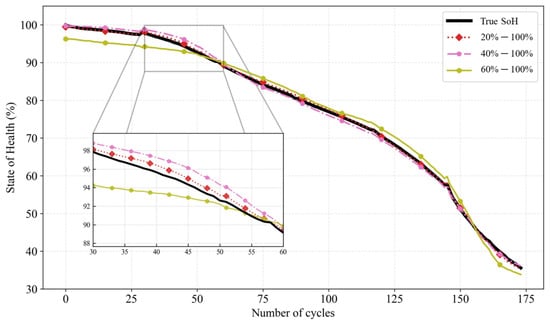
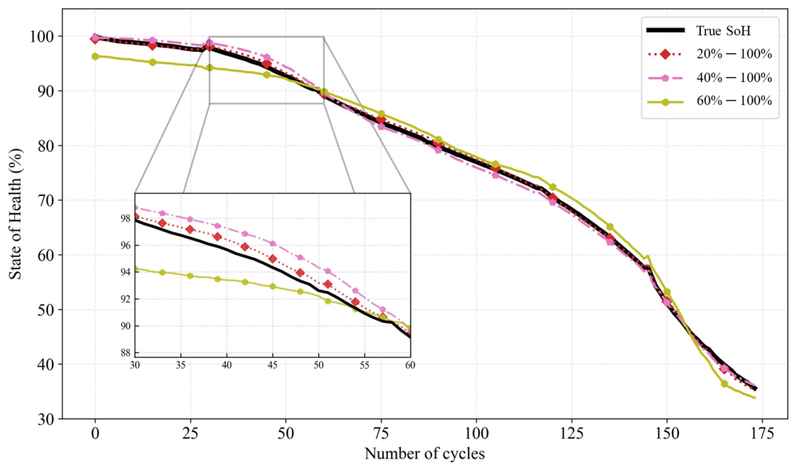
The model has been tested with different initial voltages and ranges throughout the lifetime of the testing cell. Among all the testing conditions, three have been found in which the model has been able to estimate the SoH with considerable accuracy throughout the testing cell life cycle: SoC 20–100%, 40–100%, and 60–100. Again, the SoC used here is only for easier demonstration of the terminal voltages, as the actual model inputs are the terminal voltages and the SoC values that have been considered are merely indicating the SoCs at that moment if the terminal voltages have been considered as the OCVs. The actual SoC values would be much smaller considering the 1C cycling condition because of the ohmic drop of the terminal voltage compared to the OCV. The performance evaluation for all three combinations has been shown in Figure 4. The performance matrices used for quantification have been shown in Equations (13)–(15).

$$\mathrm{RMSE}=\sqrt{{\displaystyle \frac{1}{N}}{\sum }_{k=1}^N{\left(\widehat{y_k}-y_k\right)}^2}$$

(13)

$$\mathrm{MAE}={\displaystyle \frac{1}{N}}{\sum }_{k=1}^N\left|\widehat{y_k}-y_k\right|$$

(14)

$$\mathrm{MAPE}={\displaystyle \frac{100}{N}}{\sum }_{k=1}^N{\displaystyle \frac{\left|\widehat{y_k}-y_k\right|}{y_k}}$$

(15)

Figure 4. SoH estimation performance considering different initial voltages and voltage ranges.

The estimation of SoH, while considering the full CC-charging information, in our case, from 20 to 100% SoC, the model shows notable resilience towards different degradation mechanisms throughout the life cycle, which is why the estimation accuracy is very high. The root mean square error (RMSE) that we found is 0.006, with the mean-absolute-percentage-error of 0.64%. As we increase the initial voltage consideration, the accuracy drops. It is important to note that the accuracy is significantly lower during the knee points when the battery exhibits exponential degradation compared to the linear degradation phases while considering higher starting voltage. The initial knee point at around the 40th cycle holds the least accuracy compared to the later one at around the 140th cycle. Since SEI layer growth at the anode is a dominant degradation mechanism at the beginning of life, this is a plausible explanation for the reduced estimation accuracy at the first knee point [35,36]. This is consistent with the loss of lithium inventory (LLI) dynamics introduced in Section 1, as SEI growth progressively consumes cyclable lithium and alters the low-voltage portion of the charging profile. Moreover, as lithium plating becomes the prevalent degradation mechanism towards the end of life, the upper portion of the voltage profile with higher SoCs will also get the hit, resulting in more accurate estimation with less information. Lithium plating similarly manifests as an LLI-driven effect concentrated in the higher-SoC region of the profile, consistent with the degradation mechanisms discussed in Section 1.

While considering the voltage range from SoC 60–100%, the estimation becomes highly inaccurate during the initial phases of degradation, most probably for the same reason as described for the SoC 40–100% range. However, it can somewhat follow the true value of the capacity fading as the cell cycles more. For all the other combinations, they either give better estimations for the initial phases of degradation or the final phases of degradation, depending on the range and initial voltage considerations. More details regarding their performance of different capacities have been described in the next section.

3.2. Robustness Analysis

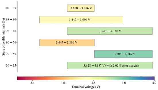
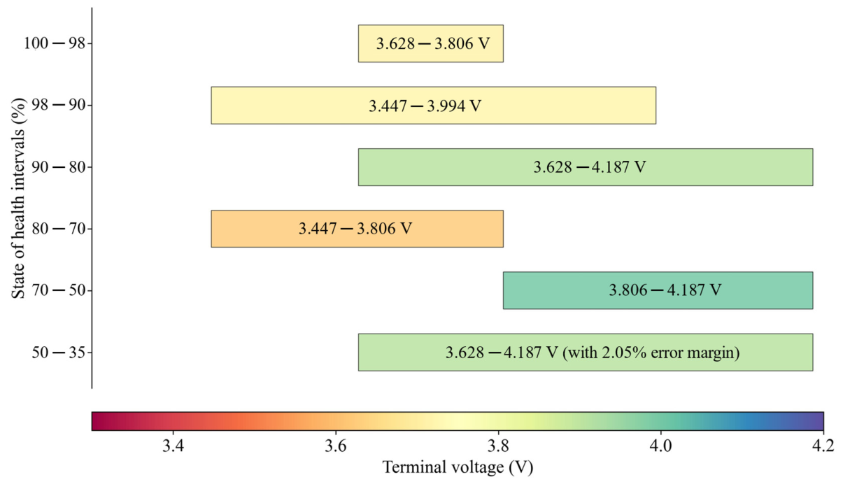
The SoH estimation models need to be robust and resilient over different voltage intervals and ranges, as well as initial voltage considerations. To test this, in this study we present a protocol where we tested the model over different SoH intervals to get the best range and initial voltage combinations for that specific SoH interval. The protocol counts the correct predictions with ≤1% absolute percentage error with respect to the true SoH and selects the optimal range with initial voltage that achieves 80% or more accuracy. The results are accumulated in Figure 5.

Figure 5. The terminal voltage initiation and range dependency of the accurate SoH estimation at different phases of degradation over the lifetime of the testing cell.

Figure 5 illustrates how the significance of different parts of the voltage profile shifts with the SoH degradation. Unlike Figure 4, the range has been illustrated based on the terminal voltage, which is the actual input for the model. For a new cell, a very narrow range of CC-charging segments can be sufficient for accurate SoH estimation. However, as the cell degrades down to 90%, a larger window of the CC-charging profile is necessary for correct estimation. From 80 to 90% of SoH, the cell almost exhibits linear degradation, which can be covered by the top portion of the CC-charging profile, disregarding the lower initial voltage values. Although the SoH from 70 to 80% still falls under the linear degradation region, it can be considered as the pre-knee arrival conditions and the batteries in such conditions have mostly been considered as SLBs, which can also be seen by the increased significance of the lower initial voltage considerations. The region of SoH from 50 to 70% is the last knee region where the higher SoC ranges are the most prominent features, most probably due to acute anodic degradation because of particle fracture [35]. The last part of life requires wider intervals, but even with that, they were unable to achieve a lower error margin than 2%.

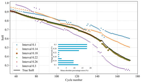
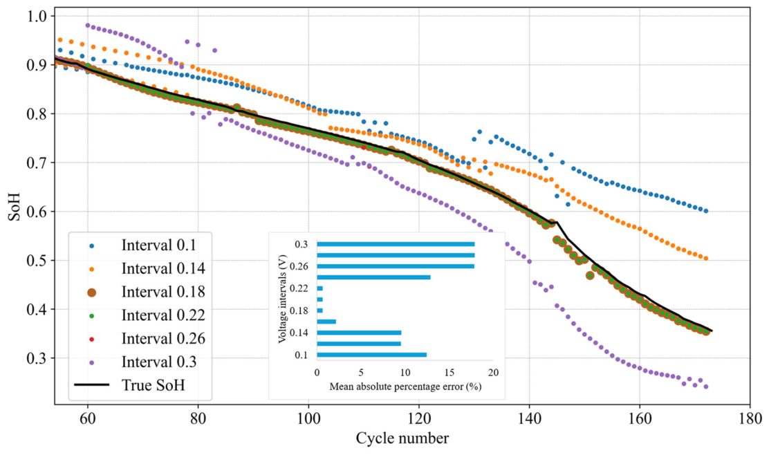
To evaluate the robustness of the proposed method, the model has been tested under 10 different sampling intervals, from 0.1 V to 0.3 V with a uniform 0.02 V gap in between, for the suggested voltage ranges for different SoH regions below 90% of the testing cell, as shown in Figure 6. This demonstrates a decrease in accuracy as the sampling interval deviates from 0.18 V, which is the lowest voltage sampling interval for the combinations that have been considered for training the model. Again, increasing the interval increases the error, showing that the proposed LSTM model is getting fewer segments to extract the temporal dependencies from the voltage profile.

Figure 6. Performance evolution under different intervals of voltage sampling, considering the suggested ranges for different SoH regions from moderate to high degradation zones.

This information is crucial to generate the final framework, where we present a suggestive approach in which the terminal voltage window consideration, as well as the initial voltage value for estimation purposes, will be suggested based on the previous SoH estimation by the presented model.

3.3. Edge-Friendly Pipeline Preparation

After proper training and evaluation of the presented model, the trained weights can be implemented on edge BMSs without any complex packages. However, it is necessary to understand how the complete framework should operate in a system. Later in this section, the details regarding the workflow of the presented framework have been elaborated.

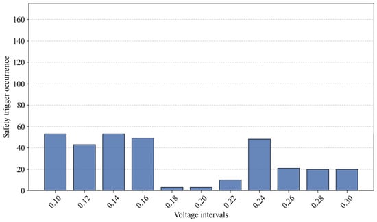
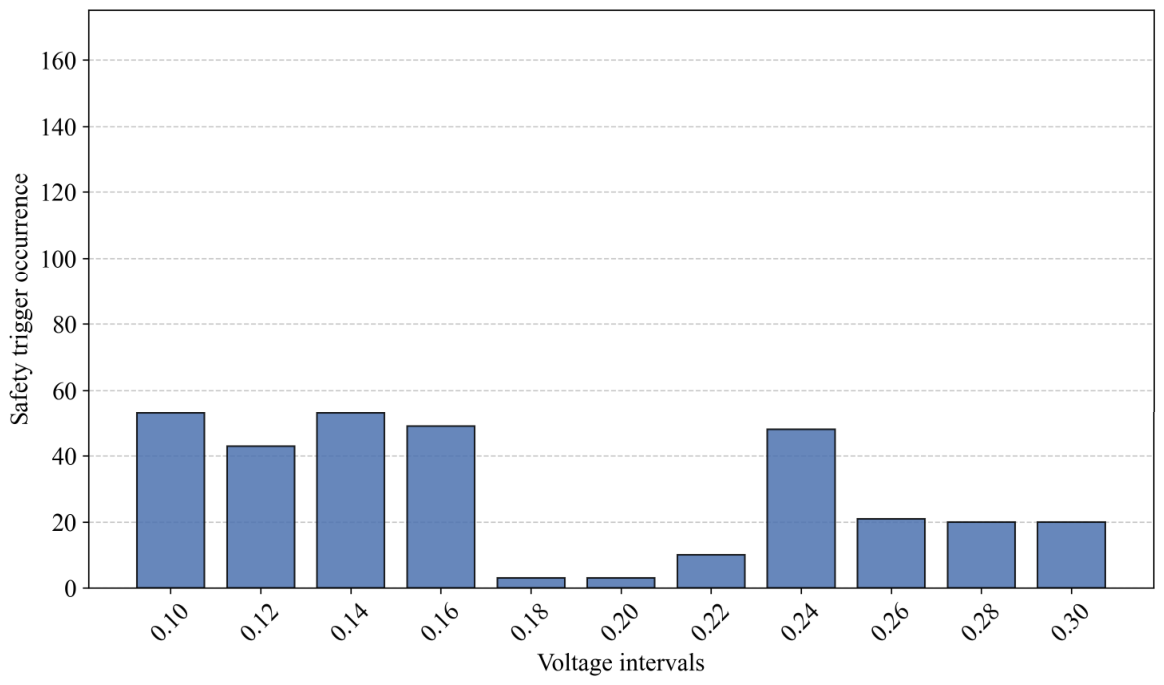
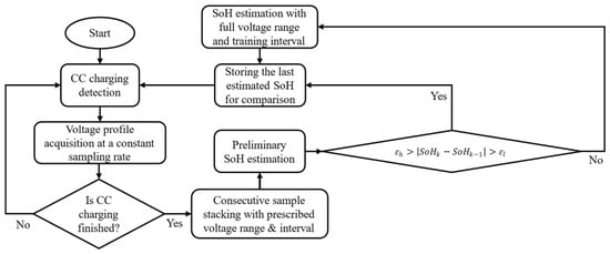
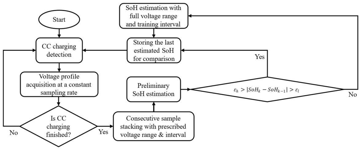
Upon deploying the model to a BMS, it will try to look for the CC-charging phase. Once the charging starts, the framework will store the initial terminal voltage and keep tracking it until it passes a certain voltage interval. The trained model is flexible towards various initial voltages and sampling intervals as inputs, with the best performance around the lowest sampling interval and predefined initial voltages used to train the model. As the input ranges deviate significantly from the trained ones, the model falls short in achieving accurate SoH estimations, thus requiring the periodic complete charge-profile-based tuning identified as the safety trigger occurrence in this manuscript, as shown in Figure 7. Here, the safety trigger occurrence refers to a schedule where the model fails to estimate the SoH bounded by a predefined limit compared to the immediately previous estimation while utilizing the suggested initial voltage and voltage range for that specific SoH region mentioned in Figure 5; thus, it requires a complete charging profile based estimation and the best voltage sampling interval (e.g., 0.18 V) for better estimation accuracy. Upon finishing the CC-charging phase, that is, once the cell reaches the CV mode or gets disconnected from the charger, the aggregated stream of inputs of consecutive intervals will be fed to the presented model for SoH estimation. As shown in Figure 4, the best performance of the SoH estimation throughout the lifetime can be achieved if the full CC-charging profile is considered, that is, from the lowest to the highest SoC. The lowest SoC of operation has been considered as 20%, and the highest is 100%. But as mentioned earlier, the battery would not be charged to its maximum range every time. So, keeping in mind the empirical situations, we presented a degradation gradient-limiting approach. As the cell observes capacity fading much slower, a threshold can be set based on battery chemistry, charge rate, and operating temperature. In this study, a 1C cycling rate at 15 °C shows a maximum capacity fading gradient of 70 mAh. (e.g., the maximum SoH gradient is ${\mathrm{\epsilon }}_h=0.02$). For this reason, after the SoH estimation for each cycle, the gradient for the SoH has been considered with respect to the previous estimation. If the gradient passes the limit of ${\mathrm{\epsilon }}_h$, that measurement will be discarded and the system will wait until it gets the full CC-charging profile for the best estimation. Again, based on the C-rate of the cycling and operating conditions, there should be a minimum capacity fading gradient for the battery. In this study, the minimum capacity fading gradient has been found to be 5 mAh (e.g., the minimum SoH gradient is ${\mathrm{\epsilon }}_l=0.0015$), and if the estimated SoH falls below this threshold, the system will again wait for the complete CC-charging data and estimate based on that. The complete framework architecture is shown in Figure 8.

Figure 7. Safety trigger occurrence during different voltage sampling interval considerations among 174 cycles of the testing cell for the presented framework.

Figure 8. Implementation flowchart of the presented framework.

3.4. Discussion

The presented ensembled LSTM-based framework demonstrates strong predictive performance when compared to several recent hybrid models used for online SoH estimation. Specifically, the presented model achieved an exceptionally mean absolute error (MAE) of 0.0038. This represents a notable improvement over other architectures evaluated in the comparative analysis, such as the CNN + Random Forest model [16], which reported an MAE of over 0.62%, and the LSTM-RNN model, which reported an MAE of over 0.64% [18]. Furthermore, the presented ensembled LSTM model attained a high R² value of 0.999, closely comparable to the R² of 0.97 reported for the CNN + Self-Attention model [17]. While that model achieves a lower RMSE (0.0043 vs. 0.005 for the presented framework), it relies on a substantially more complex architecture and a narrow, fixed CC window (80–97% SoC), whereas the presented framework maintains competitive accuracy across a far wider and more flexible range of partial charging intervals.

A primary operational advantage of the presented framework lies in its flexibility regarding initial voltage and window of consideration. The presented architecture processes a consecutive suggestive window-based CC charge profile. This methodology is significantly less restrictive than the CNN + Self-Attention model, which relies on a very narrow CC window constrained strictly between 80 and 97% SoC. Furthermore, the presented algorithm avoids the stringent data requirements of models that necessitate full charging data, such as the LSTM-RNN model (which requires the full CC charging process and fixed-length health indicator (HI) segments) and the CNN + Random Forest model (which requires CC–CV health features from a full charge cycle) [16,18]. While the stacking ensemble model (GPR + RBFNN + SVR + RF) also accommodates variable-length partial CC charging segments and achieved competitive performance, the error accumulation over cycles due to the previous discharge curve dependency, as well as the requirement for higher-resolution sensors due to ICA acquisition, are the main disadvantages when considering the presented framework in this study. Moreover, none of the existing approaches considered the non-linear SoH degradation efficacy, unlike the presented framework, which has also been evaluated over knee point degradation of the testing cell, covering a wide range of SoH limits, which shows the feasibility of the presented framework in second-life battery applications too.

Finally, it should be noted that the comparative models were validated on various public datasets, including Stanford LFP, NASA, CALCE, and Oxford cells. As such, direct numerical comparison across datasets should be interpreted with some caution, given differences in cell chemistry, aging protocol, and data collection conditions; the comparison is intended to contextualize relative performance trends rather than claim strict equivalence. Table 3 shows comprehensive comparisons of the presented framework over the existing approaches.

Table 3. Comparative analysis of recent hybrid models for online battery SoH estimation utilizing variable-interval SoC charge profiles.

Ref.	Architecture	SoC Interval/Feature Window	Dataset	RMSE	MAPE (%)	MAE	R2
[17]	CNN + Self-Attention	Narrow CC window (80–97% SoC)	Stanford LFP; 222 cells; 146,074 cycles	0.0043	0.354	-	0.97
[18]	LSTM-RNN	Full CC charging process; fixed-length HI segments	NASA; CALCE	<1.00%	-	0.64–0.95%	-
[24]	Stacking Ensemble (GPR + RBFNN + SVR + RF)	Partial CC charging segments (variable length)	Oxford and NASA datasets	0.41–<1%	-	0.39–<1%	-
[16]	CNN + Random Forest	CC–CV health features; full charge cycle	CALCE (multi-cell, cross-condition)	-	-	>0.62%	-
This work	Ensembled LSTM	Consecutive suggestive window-based CC charge profile	Custom aging dataset	0.005	0.634	0.0038	0.999

4. Conclusions

This study sets out to determine whether reliable SoH estimation can be maintained amidst the highly variable and unpredictable charging characteristics of real-world EV operation. By abandoning the rigid constraints of fixed-window and fixed-starting-voltage assumptions that traditionally underpin laboratory-grade models, the proposed LSTM ensemble framework demonstrates that partial, consecutively sampled constant-current charge profiles retain sufficient degradation signatures. This approach enables the delivery of accurate enough SoH estimates without requiring a complete charge cycle from a predefined initial SoC or a specific quantity of charging.

The practical utility of this framework lies not in any single design choice, but in the synergetic integration of its components. The nested voltage intervals dynamically adapt to compensate for aging-induced changes, while the mapping strategy enables the BMS to consistently isolate the most diagnostically informative segments. Furthermore, the resulting model, comprising a mere 474 parameters and requiring less than 30 KB of memory, is fully deployable in pure NumPy, demanding no hardware modifications beyond what is already present in standard controllers. The input feature set can also be extended with additional scalars such as ambient temperature and charging C-rate, allowing the framework to generalize beyond the fixed 15 °C/1C conditions validated here without changes to the model architecture. Moreover, the training dataset can be expanded in future work to cover other ranges effectively to make the proposed architecture more flexible and resilient towards variable multi-intervals with arbitrary initial voltages. Experimental validation across four commercial INR18650MJ1 cells, tested rigorously through the capacity knee point and well into second-life territory, confirms the robustness of these properties under non-idealized, full-lifecycle conditions.

Ultimately, this framework bridges a critical deployment gap rather than a purely technical one. While high-accuracy SoH estimation is well-documented in the existing literature, models that simultaneously survive irregular charging profiles, execute efficiently on legacy BMS hardware, and maintain fidelity past 1st life retirement remain exceedingly rare. This unique combination of algorithmic resilience and computational efficiency positions the proposed approach as a scalable, production-ready foundation, rather than a mere proof of concept for the next-generation battery management in existing EV fleets.

References

- Zhu, R.; Shaukat, H.; Zahira, F.; Huzefa, H.M.; Bin Kaleem, M.; Li, H. State-of-Health Estimation for Li-Ion Batteries of Real-World Electric Vehicles: Progress, Challenges, and Prospects. Batteries 2026, 12, 174. [Google Scholar] [CrossRef] [Scilit]
- Bustos, J.E.G.; Schiele, B.B.; Baldo, L.; Masserano, B.; Jaramillo-Montoya, F.; Troncoso-Kurtovic, D.; Orchard, M.E.; Perez, A.; Silva, J.F. In Situ Estimation of Li-Ion Battery State of Health Using On-Board Electrical Measurements for Electromobility Applications. Batteries 2025, 11, 451. [Google Scholar] [CrossRef] [Scilit]
- Abu Qahouq, J.A. An Electrochemical Impedance Spectrum-Based State of Health Differential Indicator with Reduced Sensitivity to Measurement Errors for Lithium–Ion Batteries. Batteries 2024, 10, 368. [Google Scholar] [CrossRef] [Scilit]
- Ketjoy, N.; Mensin, Y.; Mensin, P.; Kaewpanha, M.; Khakhu, S.; Chantarapongphan, C.; Sulaiman, S.I. Development of a Degradation Model for Lifespan Prediction: A Case Study on Grid-Scale Battery Energy Storage Systems in Thailand. Batteries 2025, 11, 429. [Google Scholar] [CrossRef] [Scilit]
- Madani, S.S.; Shabeer, Y.; Nair, A.S.; Fowler, M.; Panchal, S.; Ziebert, C.; Chaoui, H.; Dou, S.X.; See, K.; Mekhilef, S.; et al. Advances in Battery Modeling and Management Systems: A Comprehensive Review of Techniques, Challenges, and Future Perspectives. Batteries 2025, 11, 426. [Google Scholar] [CrossRef] [Scilit]
- Zhang, C.; Kang, Y.; Duan, B.; Zhou, Z.; Zhang, Q.; Shang, Y.; Chen, A. An Adaptive Battery Capacity Estimation Method Suitable for Random Charging Voltage Range in Electric Vehicles. IEEE Trans. Ind. Electron. 2022, 69, 9121–9132. [Google Scholar] [CrossRef] [Scilit]
- Gholaminejad, A.; Mohammad-Alikhani, A.; Nahid-Mobarakeh, B. A Hybrid End-to-End Dual Path Convolutional Residual LSTM Model for Battery SOH Estimation. Batteries 2025, 11, 449. [Google Scholar] [CrossRef] [Scilit]
- Peng, S.; Sun, Y.; Liu, D.; Yu, Q.; Kan, J.; Pecht, M. State of Health Estimation of Lithium-Ion Batteries Based on Multi-Health Features Extraction and Improved Long Short-Term Memory Neural Network. Energy 2023, 282, 128956. [Google Scholar] [CrossRef] [Scilit]
- Neunzling, J.; Hainke, P.; Winter, H.; Henriques, D.; Fleckenstein, M.; Markus, T. Investigation of the Suitability of the DTV Method for the Online SoH Estimation of NMC Lithium-Ion Cells in Battery Management Systems. Batteries 2025, 11, 25. [Google Scholar] [CrossRef] [Scilit]
- Dai, Y.; Liu, X.; Li, H.; Liu, X.; Zhang, T.; Su, Z.; Zhao, S.; Zhou, Y. Building-Related Electric Vehicle Charging Behaviors and Energy Consumption Patterns: An Urban-Scale Analysis. Transp. Res. Part D Transp. Environ. 2025, 141, 104663. [Google Scholar] [CrossRef] [Scilit]
- Koleti, U.R.; Rajan, A.; Tan, C.; Moharana, S.; Dinh, T.Q.; Marco, J. A Study on the Influence of Lithium Plating on Battery Degradation. Energies 2020, 13, 3458. [Google Scholar] [CrossRef] [Scilit]
- Long, Z.; Chen, K.; Tang, M.; Zheng, X.; Wang, H.; Luo, Y.; Li, Y.; Nie, G.; Zhang, X.; Gao, G.; et al. A Review of Modeling the Aging Mechanism of LIBs: Multi-Physics Field Coupling Analysis from LLI to LAM. Int. J. Green Energy 2026, 23, 1546–1573. [Google Scholar] [CrossRef] [Scilit]
- Liu, H.; Naqvi, I.H.; Li, F.; Liu, C.; Shafiei, N.; Li, Y.; Pecht, M. An Analytical Model for the CC-CV Charge of Li-Ion Batteries with Application to Degradation Analysis. J. Energy Storage 2020, 29, 101342. [Google Scholar] [CrossRef] [Scilit]
- Zhang, C.; Luo, L.; Yang, Z.; Du, B.; Zhou, Z.; Wu, J.; Chen, L. Flexible Method for Estimating the State of Health of Lithium-Ion Batteries Using Partial Charging Segments. Energy 2024, 295, 131009. [Google Scholar] [CrossRef] [Scilit]
- Qian, K.; Li, Y.; Zou, Q.; Cao, K.; Li, Z. SOH and RUL Estimation for Lithium-Ion Batteries Based on Partial Charging Curve Features. Energies 2025, 18, 3248. [Google Scholar] [CrossRef] [Scilit]
- Yang, N.; Song, Z.; Hofmann, H.; Sun, J. Robust State of Health Estimation of Lithium-Ion Batteries Using Convolutional Neural Network and Random Forest. J. Energy Storage 2022, 48, 103857. [Google Scholar] [CrossRef] [Scilit]
- Zhao, J.; Li, D.; Li, Y.; Shi, D.; Nan, J.; Burke, A.F. Battery State of Health Estimation under Fast Charging via Deep Transfer Learning. iScience 2025, 28, 112235. [Google Scholar] [CrossRef] [Scilit] [PubMed]
- Liu, K.; Kang, L.; Xie, D. Online State of Health Estimation of Lithium-Ion Batteries Based on Charging Process and Long Short-Term Memory Recurrent Neural Network. Batteries 2023, 9, 94. [Google Scholar] [CrossRef] [Scilit]
- He, Y.; Deng, Z.; Chen, J.; Li, W.; Zhou, J.; Xiang, F.; Hu, X. State-of-Health Estimation for Fast-Charging Lithium-Ion Batteries Based on a Short Charge Curve Using Graph Convolutional and Long Short-Term Memory Networks. J. Energy Chem. 2024, 98, 1–11. [Google Scholar] [CrossRef] [Scilit]
- Lin, C.; Xu, J.; Shi, M.; Mei, X. Constant Current Charging Time Based Fast State-of-Health Estimation for Lithium-Ion Batteries. Energy 2022, 247, 123556. [Google Scholar] [CrossRef] [Scilit]
- Huang, B.; Xuan, Y.; Liu, X.; Liu, D. Fast Estimation Method for Lithium Battery State of Health Based on Incremental Capacity Curve Peak Characteristics. Proc. Inst. Mech. Eng. Part D J. Automob. Eng. 2025, 239, 7597–7610. [Google Scholar] [CrossRef] [Scilit]
- Deng, Z.; Hu, X.; Xie, Y.; Xu, L.; Li, P.; Lin, X.; Bian, X. Battery Health Evaluation Using a Short Random Segment of Constant Current Charging. iScience 2022, 25, 104260. [Google Scholar] [CrossRef] [Scilit] [PubMed]
- Schmitz, M.; Kowal, J. A Deep Learning Approach for Online State of Health Estimation of Lithium-Ion Batteries Using Partial Constant Current Charging Curves. Batteries 2024, 10, 206. [Google Scholar] [CrossRef] [Scilit]
- Xu, J.; Liu, B.; Zhang, G.; Zhu, J. State-of-Health Estimation for Lithium-Ion Batteries Based on Partial Charging Segment and Stacking Model Fusion. Energy Sci. Eng. 2023, 11, 383–397. [Google Scholar] [CrossRef] [Scilit]
- Graves, A.; Schmidhuber, J. Framewise Phoneme Classification with Bidirectional LSTM and Other Neural Network Architectures. Neural Netw. 2005, 18, 602–610. [Google Scholar] [CrossRef] [Scilit] [PubMed]
- Squidstat Cycler—Base Model|Admiral. Available online: https://www.admiralinstruments.com/cyclers/cycler-base-model (accessed on 30 April 2026).
- TestEquity: TestEquity Chambers TE-101H-F Humidity Chamber, −30 to 130 C, 10 to 95% RH, 120V/60Hz, TE-100 Series. Available online: https://www.testequity.com/category/Environmental-Chambers-Ovens/Temperature-Humidity-Chambers/20222-1-TE-101H-F (accessed on 30 April 2026).
- LG INR18650 MJ1 3500mAh Rechargeable Power Cell. Available online: https://imrbatteries.com/products/lg-mj1-18650-3500mah-10a-battery?srsltid=AfmBOootnONMcTSKEZvef0l-JbdD1x6knnHpTX1ra2jV31NuD-ps1vAD (accessed on 30 April 2026).
- Morrissey, P.; Weldon, P.; O’Mahony, M. Future Standard and Fast Charging Infrastructure Planning: An Analysis of Electric Vehicle Charging Behaviour. Energy Policy 2016, 89, 257–270. [Google Scholar] [CrossRef] [Scilit]
- Tang, J.; Li, Y.; Wang, S.; Xiong, B.; Li, X.; Pan, J.; Chen, Q.; Wang, P. Data-Driven State of Health Estimation Method of Lithium-Ion Batteries for Partial Charging Curves. IEEE Trans. Energy Convers. 2024, 39, 2230–2243. [Google Scholar] [CrossRef] [Scilit]
- Li, Y.; Li, K.; Liu, X.; Li, X.; Zhang, L.; Rente, B.; Sun, T.; Grattan, K.T.V. A Hybrid Machine Learning Framework for Joint SOC and SOH Estimation of Lithium-Ion Batteries Assisted with Fiber Sensor Measurements. Appl. Energy 2022, 325, 119787. [Google Scholar] [CrossRef] [Scilit]
- Chollet, F. Deep Learning with Python, 2nd ed.; Manning Publications: Shelter Island, NY, USA, 2021. [Google Scholar]
- Maas, A.L.; Hannun, A.Y.; Ng, A.Y. Rectifier Nonlinearities Improve Neural Network Acoustic Models. In Proceedings of the 30th International Conference on Machine Learning, Atlanta, GA, USA, 16–21 June 2013. [Google Scholar]
- Hochreiter, S.; Schmidhuber, J. Long Short-Term Memory. Neural Comput. 1997, 9, 1735–1780. [Google Scholar] [CrossRef] [Scilit] [PubMed]
- Edge, J.S.; O’Kane, S.; Prosser, R.; Kirkaldy, N.D.; Patel, A.N.; Hales, A.; Ghosh, A.; Ai, W.; Chen, J.; Yang, J.; et al. Lithium Ion Battery Degradation: What You Need to Know. Phys. Chem. Chem. Phys. 2021, 23, 8200–8221. [Google Scholar] [CrossRef] [Scilit] [PubMed]
- Vetter, J.; Novák, P.; Wagner, M.R.; Veit, C.; Möller, K.C.; Besenhard, J.O.; Winter, M.; Wohlfahrt-Mehrens, M.; Vogler, C.; Hammouche, A. Ageing Mechanisms in Lithium-Ion Batteries. J. Power Sources 2005, 147, 269–281. [Google Scholar] [CrossRef] [Scilit]
Disclaimer/Publisher’s Note: The statements, opinions and data contained in all publications are solely those of the individual author(s) and contributor(s) and not of MDPI and/or the editor(s). MDPI and/or the editor(s) disclaim responsibility for any injury to people or property resulting from any ideas, methods, instructions or products referred to in the content. |
© 2026 by the authors. Licensee MDPI, Basel, Switzerland. This article is an open access article distributed under the terms and conditions of the Creative Commons Attribution (CC BY) license.