


Abstract
Metallic particle contaminants have been shown to have a detrimental effect on the reliability, performance and capacity of lithium-ion battery cells. In addition, they pose a significant safety risk. Typical contaminants, such as iron (Fe), copper (Cu) and aluminium (Al), often enter the cell via mechanical abrasion from production equipment, as burrs during electrode cutting, or through environmental exposure during handling. In such instances, the degradation mechanisms are known to accelerate, dendrite formation is increased, and, in the most unfavourable circumstances, thermal runaway is the likely outcome. Contaminants that do not affect cell behavior during formation and the initial cycles, yet only compromise safety at a subsequent stage, are of particular concern. Affected cells are known to pass end-of-line testing and make their way into the market as latent safety risks. Consequently, there is an urgent requirement for non-destructive diagnostic methods that are capable of identifying latent defects. The issue under discussion is approached in the present paper through the utilization of an innovative methodology that integrates the distribution of relaxation time (DRT) analysis of electrochemical impedance spectroscopy (EIS) data with machine learning techniques. The objective of this integrated approach is to facilitate the detection of critically contaminated pouch cells with a high degree of sensitivity.
1. Introduction
The presence of metallic particles in lithium-ion battery cells represents a significant safety and reliability concern, as even trace amounts can critically impair cell integrity. Metallic contaminants such as iron (Fe), copper (Cu), or aluminum (Al) can penetrate the separator and establish an unintended conductive path between the anode and cathode. This may result in internal short circuits, which can trigger thermal runaway, a self-sustaining exothermic reaction that poses a serious risk of fire or explosion [1,2,3,4,5].
Beyond immediate safety hazards, metallic particles can also contribute to long-term degradation mechanisms. Over time, these particles may dissolve into the electrolyte and redeposit as conductive dendrites, which can grow through the separator and eventually cause delayed short circuits [1,2,6]. Even in the absence of catastrophic failure, such contamination accelerates cell aging and leads to diminished electrochemical performance. The primary sources of metallic particle contamination include: (a) manufacturing equipment wear (abrasion from cutting tools, rollers, or other mechanical components during electrode processing), (b) electrode cutting operations (formation of burrs or fragments from copper or aluminum foils during slitting, punching, or tab welding), or (c) environmental exposure (introduction of airborne particles or dust during handling, assembly, or packaging in insufficiently controlled environments) [1,2,5].
It is therefore of great importance for cell manufacturers to implement effective strategies to either avoid particle contamination by effective detection and removal methods or to recognize already contaminated cells as rejects in a timely manner and segregate them accordingly [5]. A significant challenge arises from the fact that defective cells, provided that a particle does not cause a hard short circuit right after fabrication, can typically go through the formation process and be operated initially without any restrictions. The inherent risk only emerges at a later, unforeseeable point in time when the cell is already in use by the end customer [4]. Non-destructive quality testing and the detection of contaminated cells is therefore of immense importance. Several advanced techniques are being developed for non-destructive end-of-line detection, such as in-line X-ray inspection systems allowing detection of metallic particles as small as 20 μm in electrode plates, scanning Electron Microscopy (SEM) with EDX for detailed analysis of particle composition and 3D structure, or computed tomography (CT) for high-resolution imaging of internal structures [1,2,7]. Another powerful analytical technique with great potential for use in non-destructive quality assurance is electrochemical impedance spectroscopy (EIS). EIS can provide great insight in an electrochemical system, e.g., parameters for diffusive, inductive and capacitive effects can be determined [8]. Therefore, EIS finds application in many research areas, most of which are related to electrochemistry, such as batteries [9,10], electrocatalysts [11], corrosion [12], diffusion [13], but also in other areas like pool water quality [14], biosensors [15,16,17], and in regards to plant physiology of, e.g., eggplants [18]. It was shown by Heins et al. [19] that the application of EIS can be suitable for clarifying the relationship between the production properties of battery cells, in particular the accuracy of electrode alignment, and the long-term stability of large-format lithium-ion cells.
In principle, impedance Z is defined as the quotient of a complex voltage U and current I.
where j is the imaginary unit and is the phase shift.
The impedance spectrum displays a multitude of superimposed physical–chemical processes taking place in the battery cell, such as those occurring at the electrode surface, at the electrode–electrolyte interface and during ion transport within the electrode material and electrolyte. These processes depend on the materials used and the cell architecture, and are therefore also affected by particle contaminants and their mechanical and electrochemical impact on the cell. In general, an impedance spectrum is evaluated using an equivalent circuit (EC) fitting [8,20]. The equivalent circuit is constituted of simple passive components (e.g., resistors, capacitors, constant phase elements, or diffusion-related elements). To illustrate, an electrode surface can be represented by an RC element. An RC element is a parallel circuit comprising a resistor, which characterizes the resistance of the charge transfer process, and a capacitor, which describes the charging of the electrochemical double layer.
The impedance of a single RC element is given by
Here, R denotes the resistance, C the capacitance, and the angular frequency. The characteristic time constant corresponds to the frequency at which the imaginary part of the impedance Z reaches its peak, i.e., at [21].
In order to interpret the impedance data from the EIS measurement and identify any abnormalities, the equivalent circuit is simulated and its parameters are varied until the discrepancy between the spectra of the experiment and the equivalent circuit diagram is minimized. The reproducibility of this fitting procedure is sensitive to the choice of initial parameter estimates, since the underlying non-linear least-squares problem is inherently ill-posed and may exhibit multiple local minima [22]. Furthermore, different equivalent circuit topologies may describe the same impedance data equally well, resulting in non-unique fitting solutions [23].
Generally, the equivalent circuit is adapted to the impedance spectrum. In an optimal impedance spectrum, one peak is described by one RC element. However, the issue here is that the RC elements have similar time constants, which results in the peaks overlapping and becoming blurred. This significantly complicates the process of forming the equivalent circuit. One potential solution is to calculate the distribution of relaxation time (DRT) [8,24]. Since 2006, this method has gained increasing popularity [24]. The DRT spectrum offers a higher resolution, allowing for greater and a more accurate distinction between the peaks.
Nevertheless, in instances where the spectra of two samples exhibit minimal discrepancies, the temporal resolution of DRT analysis may be insufficient to permit a distinction to be made. In such cases, a machine learning (ML) program can be utilized to facilitate this process. These techniques have made enormous progress, even though the basic idea of ML as a method for modelling brain function has been around for a long time [25]. Since then, ML is applied in many different fields. In 2020, the largest application areas were medical imaging and cyber security [26]. Due to the exponential growth in the research field and the emergence of large language model, the largest application areas have likely changed. In battery research, machine learning approaches are increasingly being used, e.g., for the prediction of lifetime or the SOH [27,28,29,30,31].
This study presents a method comprising a combination of impedance spectroscopy, DRT analysis and machine learning, for the early detection of critical pouch cells contaminated with metal particles. The automated data analysis enables rapid classification of defect-free reference cells and defective cells with electrode stacks that are to be removed from the process chain.
2. Materials and Methods
2.1. Analytical Background: Distribution of Relaxation Times
The distribution of relaxation times (DRT) can be calculated by transferring the impedance data from the frequency domain into the time domain. This transformation is a deconvolution and an ill-posed problem [32]. Therefore, it requires a regularization to prevent overfitting. The relation between impedance Z and DRT is given by the following:
where represents the frequency-independent ohmic series resistance, comprising all purely resistive series contributions without capacitive or inductive effects. This equation is a Fredholm integral of the form [24]
In matrix form, the equation can be numerically simplified to
where is matrix that depends on the frequency. To get , the equation can be solved by
However, because the matrix is singular, the inversion of the matrix is infeasible. Therefore, a regularization is required. There exist many different regularization methods to solve ill-posed problems. This topic is not discussed in detail in this work, as there are numerous other papers dedicated to it. Herein, the Gold algorithm as presented in the paper of Bergmann and Schlueter [33] was utilized. In comparison, the Gold algorithm is more accurate than the Tikhonov regularization and more reproducible than the SparseSpike algorithm. In this iterative algorithm, the regularization parameter is the number of iterations. In the Gold algorithm, the k-th iteration is determined using the following equation:
with
When the maximum number of iterations is too high (e.g., ), the DRT becomes overfitted. Conversely, when the maximum number of iterations is too low (e.g., ) the DRT is underfitted. Further details can be found in Appendix C.
2.2. Experimental
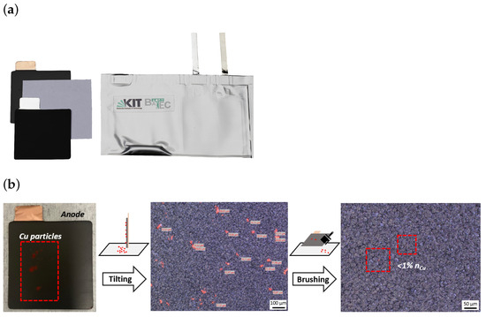
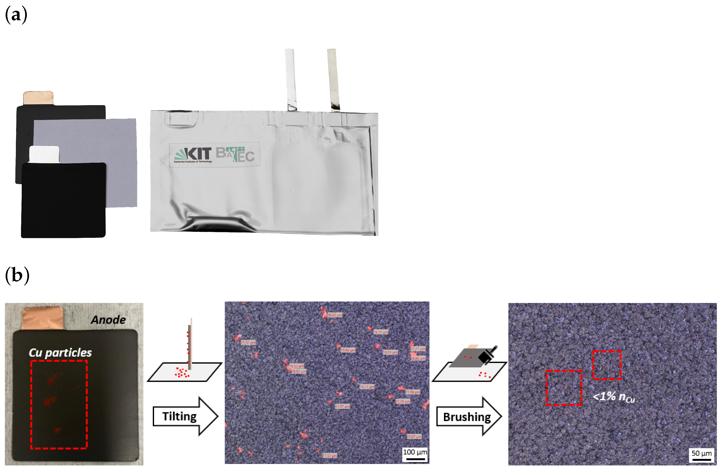
In order to facilitate the experimental investigations, Li-ion pouch cells were produced on a laboratory scale with a single-layer stack containing one anode, one cathode and one separator sheet (Figure 1a). The cells were produced in the semi-automatic cell production facility at Battery Technology Center at Karlsruhe Institute of Technology (KIT-BATEC) in a dry room (−68 °C dew point). Commercially purchased NCM622 cathodes and graphite anodes were used in size of 5.0 cm × 5.0 cm and 5.2 cm × 5.2 cm, respectively. The separator used is a commercial tri-layer PE-type with a thickness of 9 μm and 5.5 cm × 5.5 cm in size. In addition to defect-free reference cells, the electrodes of test cells were contaminated with traces of unbound Al, Cu and Fe particles before assembly. The electrodes and metal powders were subjected to a drying process under reduced pressure for a period of 24 h at a temperature of 130 °C, while the separators underwent a similar drying process under reduced pressure for a period of 24 h at a temperature of 80 °C. This was followed by the assembly of the cell stack. As part of the assembly process, a small amount of a respective metal powder was applied to one of the two electrodes. The following types of contamination were prepared: Al on the cathode, Cu on the anode and Fe on the cathode. Particle specifications including grain size distributions are given in Table 1. Photographs and microscopy images show the distribution of particles on the electrodes after the respective preparation steps exemplarily for Cu powder (Figure 1b). In addition to the type of metal, two different degrees of contamination were prepared. In both cases, a spatula tip of the appropriate powder was first dispersed on the electrode surface (see Figure 1b, left image). The electrode was then tilted by 90°, causing some of the particles to detach and be removed. This resulted in electrodes that were still clearly contaminated and will be referred to in the following as ‘high contamination’ (see Figure 1b, middle microscopy image). For another part of the samples, an additional cleaning step of the electrodes was simulated by carefully cleaning them with a brush after tilting, which removed most of the particles (see Figure 1b, right microscopy image). These samples will be referred to as ‘low contamination’. An overview of all cells tested is given in Table 2.
Figure 1.
(a) Photograph of a KIT-BATEC laboratory pouch cell with components. (b) Preparation of anode contaminated with Cu powder. Photograph of particle distribution after scattering (left) and microscopy images of particle distribution after tilting (middle) and after cleaning by brushing (right). Corresponding images of Al and Fe contaminations are provided in the Appendix A Figure A1.
Table 1.
Material specifications and grain size distributions of metal powders used as contaminants.
Table 2.
Overview of laboratory pouch cells with type and degree of contamination as well as the calculated prediction accuracy of each cell with the same (Column A). For the determination of the second prediction accuracy, cells with Al contamination were excluded from the training data (Column B).
For the formation step, the cells were operated on a BaSyTec CTS cycler at 25 °C. The first charging was performed with constant current (CC) at C/10 until a voltage of V was reached with subsequent charging at constant voltage (CV) until the current dropped to I < C/20. Then, the cells were cycled for six cycles using a CC discharge with C/2 to the lower cut-off voltage of 3.0 V and a CC-CV charge with C/2 to an upper cut-off voltage of V and until I < C/20.
After formation, the cells were further operated on a Biologic cycler (VMP3) within a climate chamber (Binder KBF-S ECO 400) at 25 °C. Prior to the EIS measurements, each cell was CC-charged to V with a current rate of C/4 followed by a CV-step until I < C/30 to allow for thermodynamic equilibration. Impedance spectra were acquired using galvanostatic electrochemical impedance spectroscopy (GEIS) in single-sine mode. A current amplitude of C/10 was applied. The spectra were recorded over a frequency range from 100 kHz to 5 mHz with logarithmic spacing at 20 points per decade. The applied potential window was set to V to V, and the current range was limited to 100 mA.
3. Results
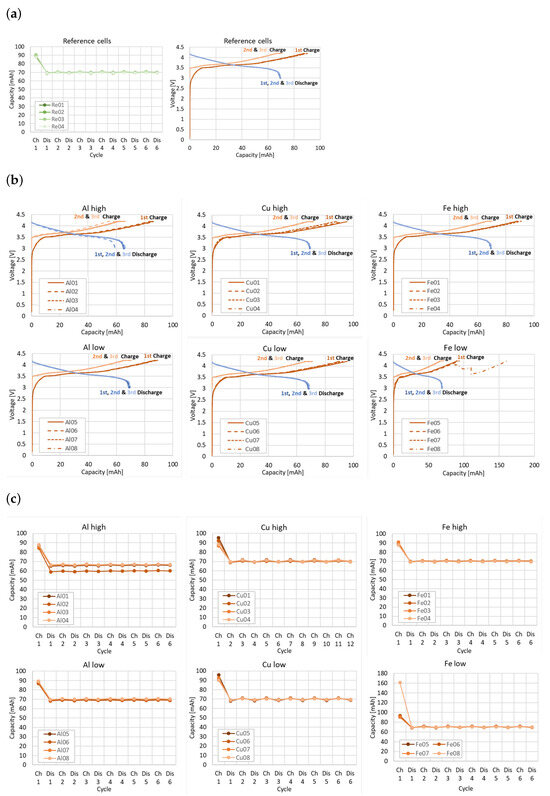
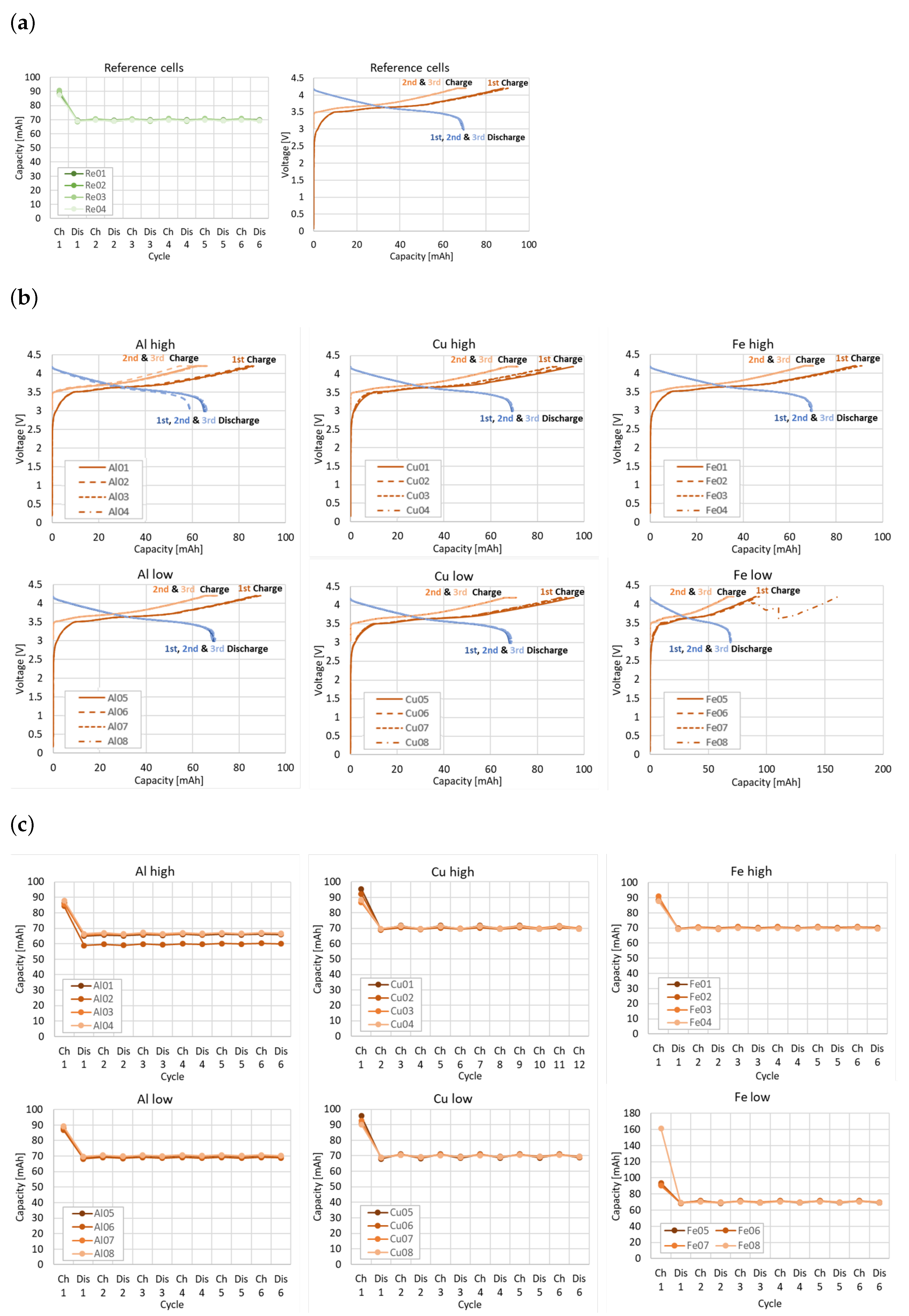
Figure 2 shows the charge–discharge curves of the formation cycles, and the capacity achieved for each cell. With the exception of a small number of outlying data points, the majority of contaminated cells exhibit no discernible deviation in performance compared to the reference cells. It should be noted that the low initial cell voltage observed for all cells prior to the first charge is a typical characteristic of freshly assembled lithium-ion cells before electrochemical activation and does not indicate defective behavior. Only the cell Al02 shows reduced capacity and the cell Fe08 shows difficulties in reaching the target charging voltage during the initial charging step. This indicates that nearly all cells containing critical particles would have remained undetected during the formation process. This observation highlights an important limitation of conventional diagnostic metrics, as standard formation data may fail to capture early-stage or subtle defect signatures caused by metallic contamination. In particular, parameters such as charge–discharge behavior alone do not provide sufficient sensitivity to reliably identify such defects at this stage. A systematic benchmarking of the proposed impedance-based method against established industrial standard tests, such as OCV tracking and self-discharge measurements, would therefore be valuable and remains an important subject of future work.
Figure 2.
(a) Charge and discharge curves and capacities of reference cells of the first three formation cycles. For the sake of clarity, reference cells Re01 to Re04 are shown. It should be noted that the other reference cells did not show any significant deviations. (b) Charge and discharge curves and (c) capacities of the first three formation cycles of defective cells.
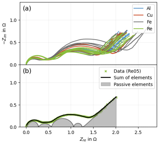
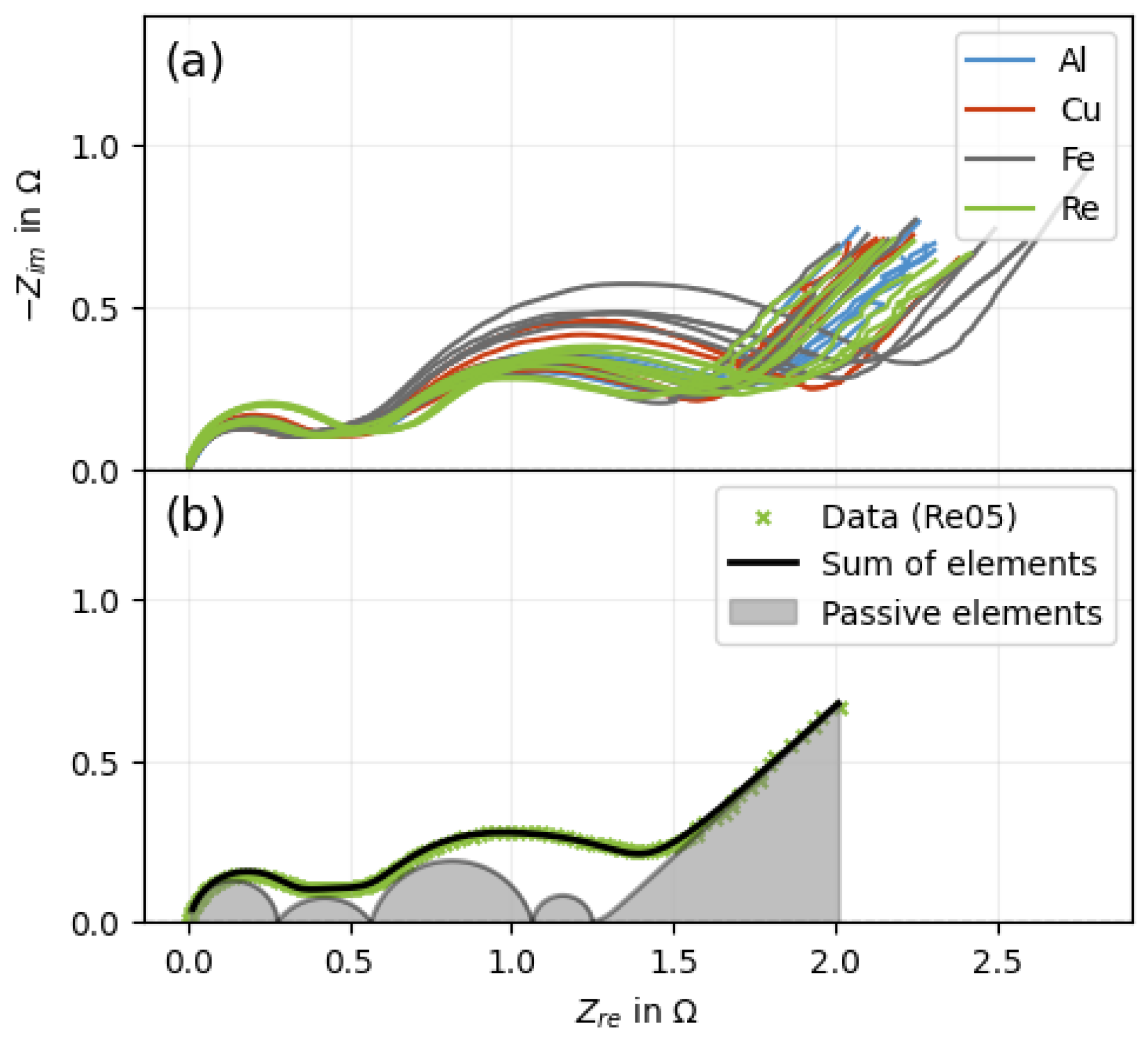
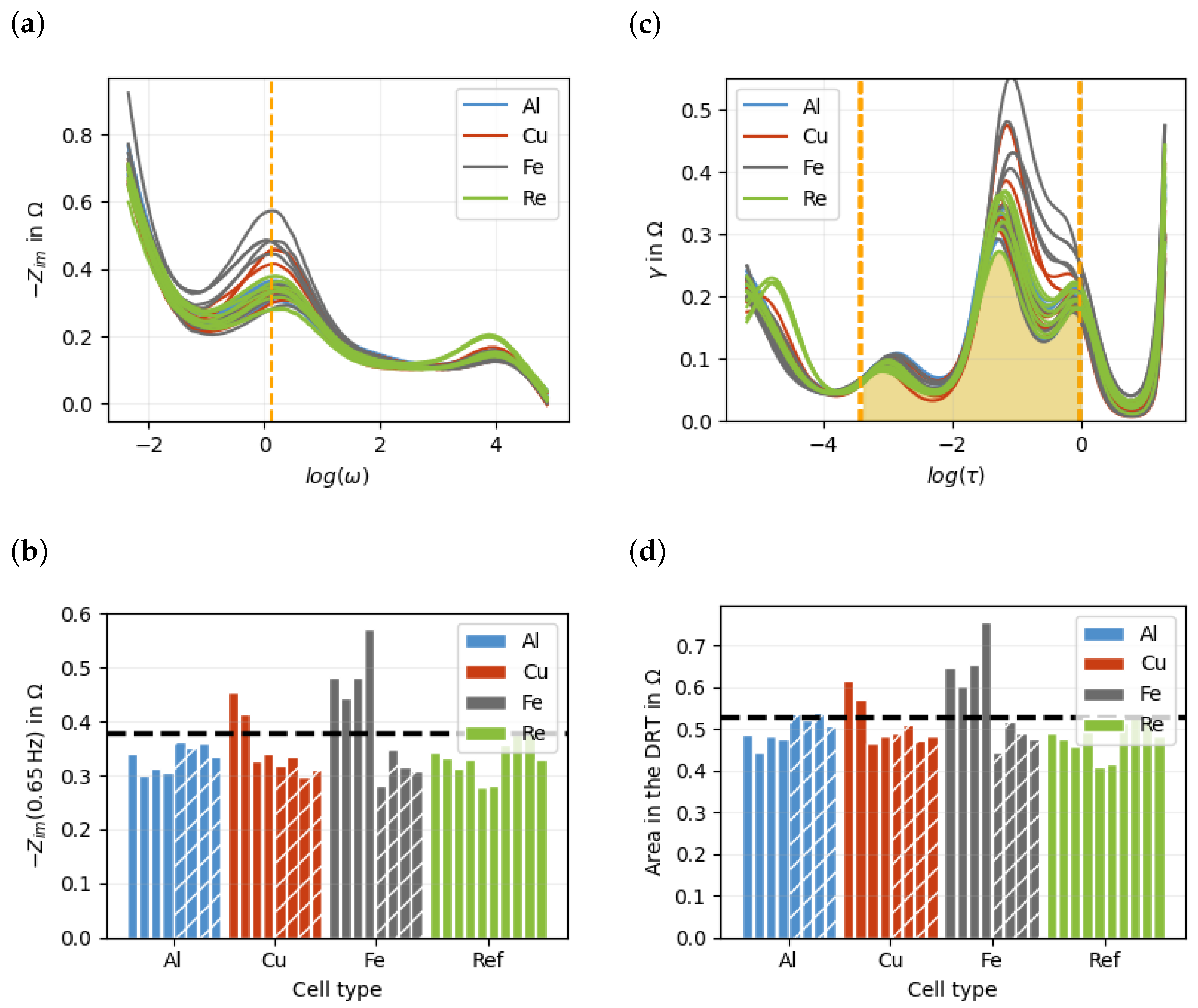
For closer examination, an impedance spectrum was measured for each cell (Figure 3a). Since the cells have slightly different series resistances that are independent of contamination, these effects were removed for each cell individually. Figure 3b illustrates the impedance spectrum of a single reference cell. A visual inspection reveals the presence of at least two semicircles. Equivalent circuit (EC) analysis reveals at least five features that can be associated to the various underlying electrochemical processes, i.e., charge transfer reactions, diffusion and double-layer charge storage. Upon initial observation, it becomes evident that all of the spectra of the reference cells in Figure 3a exhibit a comparable range, whereas the data of the contaminated cells display a more pronounced variation in terms of the position and size of the semicircles. Nevertheless, a slight variation is also present in the reference cells that is attributed to the relatively small sample size of the laboratory pouch cells. In this single-layer electrode configuration, the flexible pouch foil causes slight variations in the internal resistance. These variations arise from the comparatively small sample volume and the resulting sensitivity of the single-layer setup to mechanical and structural inhomogeneities. In multilayer electrode stacks, this effect would be significantly reduced due to better mechanical stabilization and averaging over a larger electrode ensemble. The inherent variability of the data, combined with the heterogeneity of the sample set comprising both reference cells and cells with different defect types prevents a direct classification of the measured cells into high-quality and defective categories. In order to facilitate the classification of the spectra, it is therefore necessary to reduce the number of given data points and define a simplified tolerance limit which can then be employed to classify future unknown cells. The simplest and most efficient approach is to determine the resistance at a suitable frequency that is known to deviate significantly from a tolerance range in the presence of critical contamination. If this method proves to be effective, there would be no need to measure the entire impedance spectrum. To determine the most meaningful frequency, the plot of the imaginary part as a function of the logarithmic frequency is particularly useful, as shown in Figure 4a. A comparison of the individual spectra reveals that the most significant differences between the defective and reference cells occur in the frequency range around 1.31 Hz (marked by the orange dashed line). Figure 4b shows the resistances measured at this frequency. The bars hatched with diagonal lines represent the cells with a low degree of contamination. The black line indicates the maximum resistance of the reference cells. Values above this threshold would therefore be expected for contaminated cells. However, a number of defective cells fall below this line. Although cells with a high degree of contamination tend to exhibit higher resistance values, the overlap with the reference range prevents a clear and reliable classification.
Figure 3.
(a) Impedance spectra of all cells. (b) Impedance spectrum of a reference cell (Re05) with an exemplary equivalent circuit (EC) analysis. The plot shows experimental data (green cross), the fitted response from circuit elements (black line), and the contributions of individual passive elements (shaded areas).
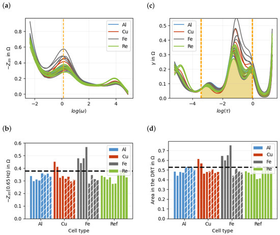
Figure 4.
(a) Imaginary impedance of each cell against the frequency. The imaginary value at the orange line showed the best classification between defective and defect-free cells. (b) Impedance value for 1.31 Hz of each cell. (c) DRT spectrum of each cell. The orange area (between and s) showed the best classification between defective and defect-free cells. (d) The resistance in the DRT spectrum between and s of each cell. The black line represent the highest reference value.
In the next step, all corresponding DRT spectra were calculated to have a visualization of the resistances plotted against the logarithmic time constants instead of frequency. All DRT spectra are presented in Figure 4c. In the graph, the area under each spectrum corresponds to the resistance of the respective cell. The Warburg impedance mainly contributes at higher time constants, approximately for , although its influence is not strictly confined to this range. In the numerically calculated DRT, this diffusion-related contribution is not represented as a single, well-defined relaxation process, but can extend over a broader range of time constants and overlap with other features, as shown in the Appendix B. To reduce its influence on the subsequent analysis, only DRT data with were considered. The Warburg impedance was not explicitly determined and subtracted using a ECM fit, as this would introduce an additional source of error and could remove information relevant for classification. Instead, the dominant high-time-constant region was truncated to reduce the risk of overfitting. The resulting DRT should therefore not be interpreted as a physically rigorous representation of the polarization processes, which would require an explicit subtraction of the Warburg contribution. The steep increase observed for is attributed to the Warburg contributions. A detailed discussion of this approach, including its limitations and the effect on the impedance reconstruction, is provided in Appendix B. Different time intervals were then systematically considered and analyzed to find a suitable interval for clear classification. It can be seen that the most significant differences in the curves occur at higher time constants around s. The interval between and s (delimited by orange lines) was identified as particularly indicative. The resistances, i.e, the areas under the curves (e.g., hatched in yellow for the cell Re05 in Figure 4b) determined in this time interval are shown in Figure 4d. It can be observed that the values of defect-free cells are significantly lower on average than those of the defective cells. Nevertheless, the tolerance limit (black dashed line), which is defined as maximum value of all reference cells, is still not sufficient for a clear classification. In the Appendix A, Appendix B, Appendix C, Appendix D, Appendix E and Appendix F, corresponding Receiver Operating Characteristic (ROC) curves can be found. Based on the DRT data, a slightly improved classification can be achieved. However, the error rate remains too high because the variability among the reference cells overlaps with the resistance values of some contaminated cells. Therefore, a simple threshold-based classification is not sufficient, motivating the use of machine learning-based approaches for a more robust separation.
The initial methodology has been shown to exhibit certain deficiencies, namely the reduction of an entire spectrum to a single data point, which effectively discards substantial additional information and relationships. Consequently, there is a necessity for an enhanced methodology. With regard to the classification process, it is imperative that the entirety of the spectrum information is utilized. Nevertheless, it is recommended to reduce the complexity of the data. To this end, principal component analysis (PCA) is performed to reduce the complexity of the DRT data while retaining the most important information. Here, each DRT spectrum is treated as one data vector consisting of 200 discretized values, where each value corresponds to the DRT intensity at a specific relaxation time. All DRT vectors are then combined into a data matrix, which is used as the input for the PCA. The original DRT spectra are thereby transformed into a new set of variables, called principal components, which describe the main variations within the spectra. The principal components were calculated using singular value decomposition (SVD), which is a mathematical method used to decompose a data matrix into orthogonal components [34]. For this purpose, the mean DRT spectrum was first subtracted from the data matrix. The SVD was then applied to this mean-centered data matrix. The resulting components define a new coordinate system in which the dominant variations between the DRT spectra are represented by the principal components.
The SVD results in three matrices, which rotate and scale the axes of the original matrix. With 34 spectra with 200 data points each, the important matrices and their dimensions are as follows:
The matrix , containing the DRT data, can be reconstructed from the new matrices (, and ). The key element of this decomposition is the rotation and subsequent sorting of the new axes () according to their respective levels of importance. This accomplishes a potential reconstruction with significant fewer axes of the entire matrix from above. The first eight principal components explain more than 95% of the total variance, while the first 15 components explain more than 99.5%. In general, the formula can be reduced to the following:
For each cell, n principal components are used to describe the 200 data points. A small n increases the data loss but simplifies the classification. However, for , the classification can no longer be performed by defining a simple threshold between two plotted principal components, since the relevant information is distributed across a higher-dimensional feature space. Therefore, machine learning models were trained to classify the cells with the matrix .
Using machine learning models always involves a risk of overfitting and underfitting. If the system is over-parameterized (e.g., with 200 data points on only 34 spectra without additional regularizations), the neural network would provide optimal results for the trained data but incorrect results for new data. This is referred to as overfitting.
To reduce this risk, suitable hyperparameters have to be selected. Hyperparameters are model settings that are defined before training and are not learned directly from the data, such as the number of principal components used as input features.
However, if the system is under-parameterized (e.g., with two data points per spectrum), the amount of data available may not be sufficient to ensure optimal classification. The model was evaluated on both DRT and impedance data. The DRT results are shown, as they demonstrated better performance.
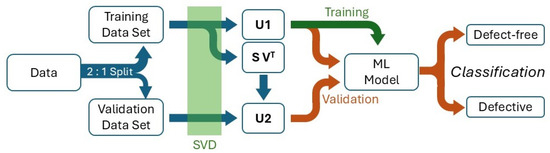
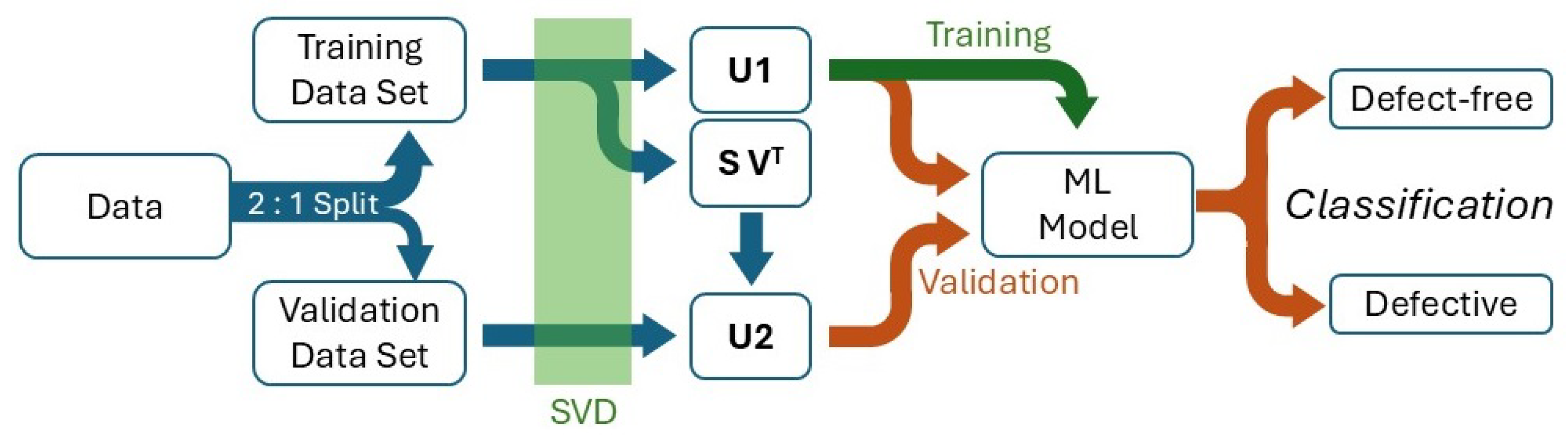
Figure 5 schematically shows the data processing carried out in this study using a machine learning model. Various machine learning models were implemented and tested using the scikit-learn package in Python. In the following, only the best-performing model is presented, while additional models can be found in the Appendix A, Appendix B, Appendix C, Appendix D, Appendix E and Appendix F. The best model consisted of a neural network utilizing the ReLU activation function. In order to prevent overfitting, an L2 regularization with a regularization parameter was employed and only a subset of selected axes of the SVD was used. In order to estimate the optimal parameters for the given dataset, a series of calculations were conducted. The mean value of 100 individual 3-fold cross-validations was determined for each parameter set. Therefore, each cross-validation had a training set of approximately two-thirds cells and a validation set of approximately one-third cells, due to the limited size of the dataset. Then the singular value decomposition (SVD) was performed on a training set , which leads to matrices , and . For the validation set , the corresponding coefficient matrix was calculated as follows:
The matrices and were reduced to a specific number of axes n before classification. Using the full matrix would result in a high-dimensional feature space compared with the limited number of measured cells, increasing the risk that the neural network learns noise, measurement fluctuations, and cell-specific variations. In particular, the later SVD axes are associated with smaller singular values and generally exhibit a poorer signal-to-noise ratio. Therefore, these components are more likely to describe low-variance noise contributions rather than robust spectral differences between defect-free and defective cells. Only the first n SVD axes were therefore used as input features to reduce overfitting and improve generalization The neural network was trained using the reduced training coefficient matrix . After the training, the model was applied to and in order to evaluate the classifcation performance on the training and validation data.
Figure 5.
Flowchart of the data processing for the analysis of experimental data using a neural network.
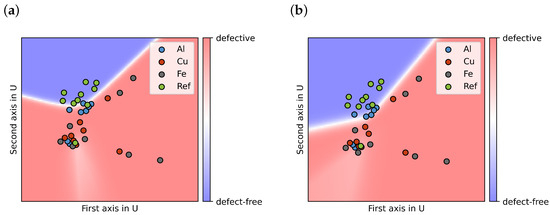
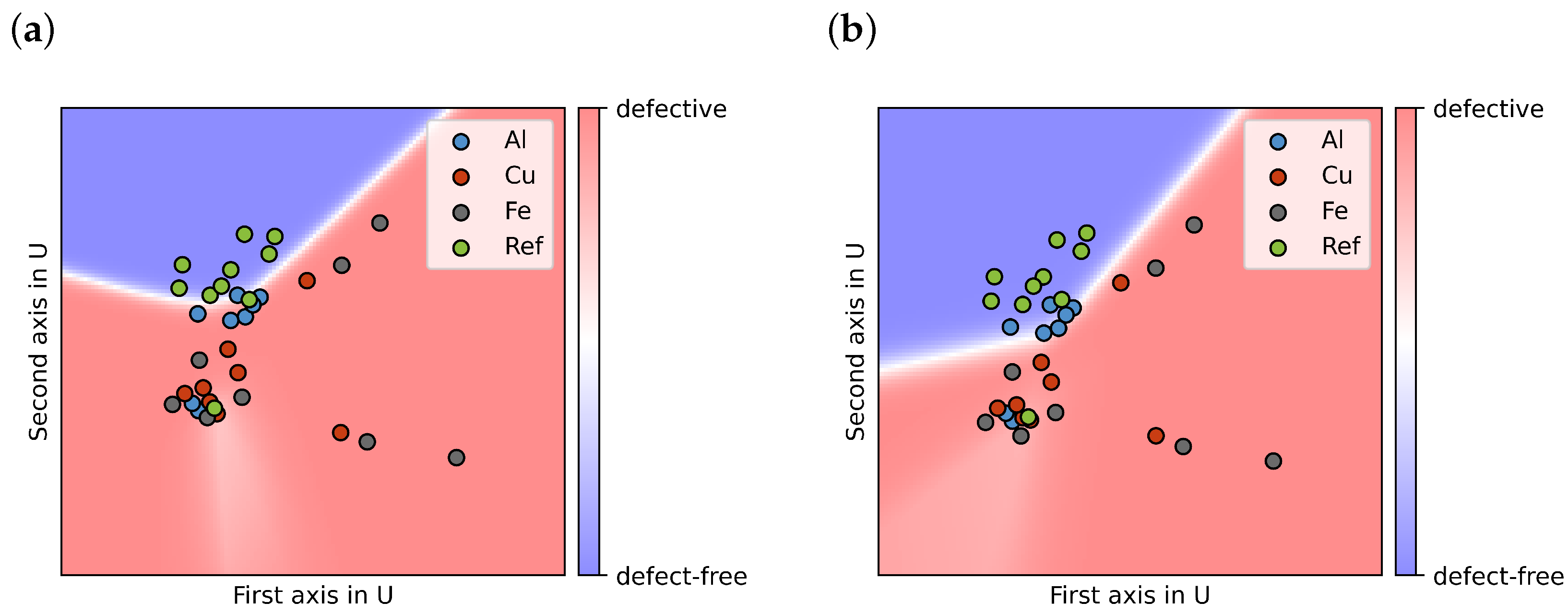
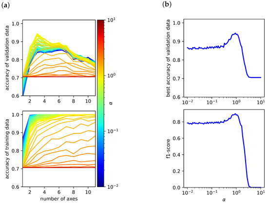
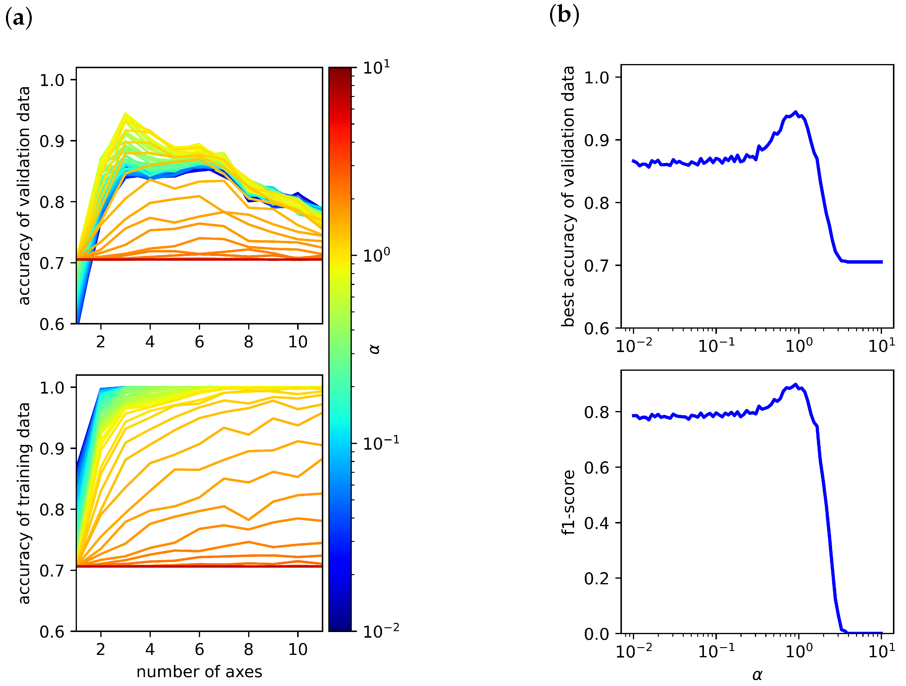
In the following, the impact of three hyperparameters was investigated: for the L2 regularization, n representing the number of axes, and the maximum iteration for the determination of the DRT. If and are reduced to two axes (n = 2), the resulting classification of the cells can be visualized as presented in Figure 6a. The resulting plot is contingent upon multiple methodological choices, including the selection of cells used for model training, the choice of activation function, the specific SVD axes considered, and the regularization parameters applied. Nevertheless, it is evident that the distinction between the two groups of reference cells and defective cells proves unattainable, underscoring the necessity for additional axes to effectively segregate the groups. The classification accuracies achieved by the ML model for the training and validation data are presented in Figure 7a. In these diagrams, the respective accuracy is plotted as a function of the number of axes included in the model. Moreover, the regularization parameter is systematically varied, with its value encoded by the colour scale.
Figure 6.
Classification of the measured cells using the first two SVD axes, showing the four different cell types indicated by the point colors. The model performs a binary classification and distinguishes only between defect-free and defective cells, not between the individual contamination types; this decision boundary is shown as blue (defect-free) and red (defective), with color intensity reflecting the prediction probability. (a) Classification result when all cell types were included in training. (b) Classification result when Al-contaminated cells were excluded from the training dataset.
Figure 7.
(a) The highest achievable accuracy for the validation and training data using the ReLU function is plotted against the number of axes n and the regularization parameter . (b) For each value of , the best possible validation accuracy and F1-score are presented.
The maximum validation accuracy is achieved for axes (Figure 7a). When fewer than three axes are used, the model exhibits clear underfitting, as evidenced by the pronounced drop in both training and validation accuracy. Conversely, when more than seven axes are included, the model enters a regime of strong overfitting. In this case, the training accuracy remains at , while the validation accuracy gradually deteriorates. In addition to the number of axes, the accuracy also strongly depends on the L2 regularization parameter . Figure 7b shows the best achievable accuracy as a function of , corresponding to the maximum value of each individual curve in Figure 7a. As expected, very small regularization strengths () result in overfitting: the model adapts overly closely to the training samples, capturing noise and spectral fluctuations rather than the underlying structure. This leads to poor generalization performance despite excellent training accuracy. In contrast, excessively large regularization parameters () cause underfitting. Strong penalization of the weights forces the network toward overly simplistic representations, preventing it from capturing relevant spectral features and degrading performance on both training and validation data. For extremely large values (), the model collapses into a trivial solution and predicts of the cells as defective, resulting in an accuracy of approximately (24/34 cells). Additionally, the f1-score for the reference cells is evaluated to account for this behavior, as accuracy alone can be misleading in the presence of class imbalance or trivial predictions. The f1-score is able to identify falsely well-performing models.
Besides the L2 regularization, additional hyperparameters influence the model performance, such as the number of neurons per layer (30–30–30) and the maximum number of iterations (). The optimal parameter set, yielding a validation accuracy of , is obtained using the ReLU activation function with and three axes of .
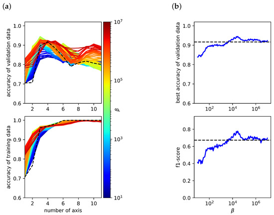
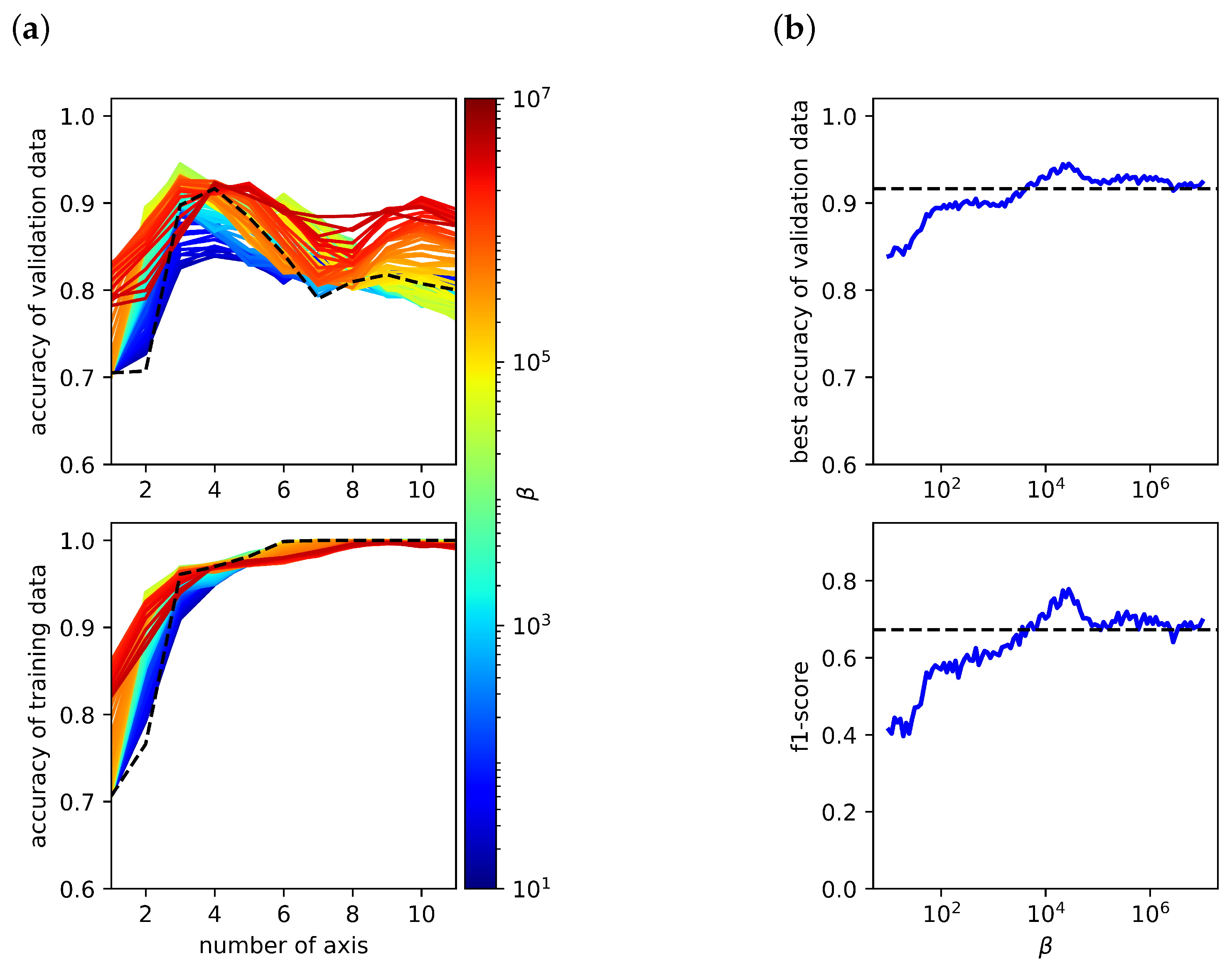
Once a suitable value of the regularization parameter had been identified and fixed, the influence of the regularization parameter was examined as presented in Figure 8. As before, a two-panel representation is used. Figure 8 is analogous to Figure 7. Here, rather than , the optimal value of is determined based on the maximum accuracy achieved for both training-data reconstruction and validation-data fitting. The analysis reveals a systematic increase of the maximum accuracy towards higher numbers of axes as the parameter increases. However, the overall best performance is achieved with and for a fixed .
Figure 8.
(a) The highest achievable accuracy for the validation and training data using the ReLU function is plotted against the number of axes and the regularization parameter . (b) For each , the best possible validation accuracy and F1-score are presented. The black line indicates the performance of a reference model for which the impedance spectrum was used directly as input, without prior DRT transformation.
The DRT representation does not introduce independent experimental information beyond the measured impedance data. Rather, it serves as a regularized feature representation that makes overlapping processes more separable. It may be possible to achieve comparable performance using the raw impedance spectra, but this would require further time-intensive model development and validation.
Finally, the classification behaviour of the individual cells was investigated. Due to the small dataset size, the classification outcome for each cell is highly sensitive to the specific split between training and test data. To reduce the variance introduced by individual data partitions and obtain more reliable estimates, each cell was evaluated using 200 independently trained models based on repeated stratified cross-validation with varying selections of test and validation cells. The classification quality was quantified in terms of accuracy, defined as the ratio of correct predicted labels to total number of predictions, aggregated over all samples from both the training and validation sets.
The resulting accuracy values for each cell are summarized in Table 2 (Column A). The reported accuracy values indicate how reliably each cell is assigned to its correct class (“defect-free” or “defective”). An accuracy of corresponds to an unambiguous and fully correct prediction. Intermediate values represent predictions with lower certainty: the smaller the value, the more frequently defect-free cells are incorrectly classified as defective and vice versa. These accuracy metrics therefore provide a direct measure of the robustness and reliability of the classification model for each individual cell. As can be seen from the values, one reference cell (Re04) exhibits a notably poor prediction. It is classified as defect-free with an accuracy of only , which corresponds to a likelihood of being predicted as defective, suggesting that this cell may indeed show characteristics associated with defective behaviour. Furthermore, several cells containing aluminum particles on the cathode (Al01–Al04) exhibit relatively low accuracy values, meaning that they tend to appear in the region typically associated with defect-free cells. This proximity to the reference cells is also clearly visible in Figure 6a. This behavior can be attributed to the rapid formation of a thin, dense, and strongly passivating Al2O3 layer on the aluminum surface under the electrochemical conditions at the cathode. Studies have demonstrated that aluminum forms a uniform and compact oxide film that substantially suppresses reactivity, thereby limiting its interaction with the surrounding electrolyte [35]. Hence, the potential misclassification of these cells is not unexpected. In contrast, Fe does not form a stable protective layer under cathodic conditions. Instead, Fe tends to generate porous and unstable oxides, allowing it to remain electrochemically active. When dissolved Fe ions enter the electrolyte, they can contribute to the formation of secondary phases or disrupt the layered structure of NCM cathodes, as previously described in the literature [36]. Its persistent reactivity further increases the risk of electrical short circuits due to the potential formation of conductive deposits. Copper is likewise thermodynamically unstable within the very low electrochemical potential window of the anode (∼0–0.1 V vs. Li/Li+). Even trace amounts of Cu at the anode can therefore pose a severe threat to cell stability. Once dissolved, copper may re-deposit in an uncontrolled manner, leading to dendritic growth and ultimately short circuits, as supported by prior studies [2].
Overall, the average accuracy across all analyzed cells is 95.93%. It should be noted, that in this study no specific cost matrix was used, as commonly applied in large-scale error classification tasks to weight different types of misclassifications. The present work serves primarily as a proof-of-concept for the proposed method. Consequently, all misclassification types were treated equally. Given that the reliable identification of faulty cells is particularly critical in industrial applications, future implementations of the proposed method should, however, consider incorporating a cost matrix or explicitly prioritizing recall during model training. This would allow the classifier to weight false negatives more strongly, thereby reducing the risk of incorrectly labeling defective cells as defect-free.
Due to the inconsistent behavior of the aluminum-contaminated cells, the modeling procedure was repeated with these samples excluded from the training dataset. The resulting accuracy of this new ML model is summarized in Table 2 (column B). The table shows that the removal of Al-contaminated samples improves the classification of reference cells, whereas the ability to correctly identify defective cells with Fe and Cu contamination is slightly reduced. The cells with Al contamination show no clear classification. This behaviour indicates that the model is sensitive to the composition and heterogeneity of the defect classes within the training set. As a consequence of excluding one defect category, the overall average accuracy decreases to . If required, this trade-off could be counteracted by incorporating an appropriate cost matrix during model training. Figure 6b presents the classification results obtained from the revised model, using the first two axes of the SVD for visualization. In the present analysis, the model performs a binary classification and differentiates only between defect-free reference cells and defective cells, independent of the specific contamination type. With a larger and more balanced dataset, however, a more granular classification strategy could be implemented, in which each defect type (e.g., Fe, Cu, or Al contamination) is treated as a distinct class.
While the presented results demonstrate the feasibility of the proposed approach, it should be noted that the experiments were conducted using single-layer pouch cells, which do not fully represent the structural and mechanical characteristics of commercial multilayer battery designs. The simplified configuration was deliberately chosen to enable a controlled and systematic investigation of the influence of metallic particle contamination, allowing the isolation of electrochemical effects associated with individual contaminants (Fe, Cu, Al) without additional complexities introduced by multilayer stacking. This approach facilitates the identification of characteristic signatures in the EIS and DRT spectra and provides a foundation for the development of data-driven classification methods. However, in multilayer cells, factors such as mechanical stabilization, interlayer interactions, and reduced variability in contact conditions may affect the impedance response and potentially reduce the sensitivity to contamination-related features. Consequently, the present study should be understood as a proof-of-concept under controlled laboratory conditions. Further validation on multilayer cell configurations and under more industry-relevant conditions will be necessary to assess the transferability and practical applicability of the proposed method. Also, it should be noted that the detection limits with respect to particle size and concentration have not yet been systematically investigated. In addition, the transferability of the proposed approach to more subtle and uniformly distributed contamination scenarios may involve reduced signal contrast in the impedance response, potentially affecting classification performance. These aspects will be essential to assess the applicability of the method under more challenging and industry-relevant conditions.
4. Conclusions
In this work, we investigated an approach for detecting particle-induced defects in lithium-ion battery cells by combining electrochemical impedance spectroscopy (EIS), distribution of relaxation time (DRT) analysis, and machine-learning techniques. Defect-free reference cells and cells intentionally contaminated with Al, Fe, or Cu particles were analyzed to evaluate a methodology capable of distinguishing non-defective from defective cells for quality-assurance applications. The DRT transformation was employed to enhance the separation of overlapping electrochemical processes in the EIS spectra and to increase the visibility of characteristic features associated with different sample conditions. While this improved spectral resolution, neither EIS nor DRT alone enabled a reliable classification of cells. To extract additional information contained in the impedance response, a DRT-based machine learning workflow was introduced. Principal component analysis effectively reduced the dimensionality of the DRT spectra while preserving the dominant electrochemical signatures, indicating that only a limited number of frequencies may be required for accurate reconstruction. Based on these principal components, a neural network was trained to differentiate between defective and defect-free cells. The machine learning model substantially outperformed conventional threshold-based methods, with the highest accuracy achieved using three principal components, a ReLU activation function, and the optimized regularization parameters and . These findings suggest that impedance measurements at only a few selected frequencies could be sufficient for reliable classification, offering a potential pathway toward faster in-line diagnostics. Overall, the results highlight the strong potential of combining advanced data-driven methods with electrochemical analysis to improve defect detection in battery cell production. However, it should be noted that the present study is based on single-layer pouch cells under controlled laboratory conditions, and the direct transferability to commercial multilayer cells remains to be validated. Future work will therefore focus on extending the approach to more complex and industry-relevant cell configurations. To further enhance model robustness and generalizability, future studies should validate the approach using larger and more diverse datasets and explore its suitability for distinguishing individual defect types.
Author Contributions
Conceptualization, T.G.B. and L.L.; methodology, T.G.B., X.L.-T., B.Z. and L.L.; software, T.G.B. and B.Z.; validation, T.G.B. and L.L.; formal analysis, T.G.B.; investigation, T.G.B. and L.L.; resources, T.G.B., X.L.-T. and L.L.; data curation, T.G.B. and L.L.; writing—original draft preparation, T.G.B. and L.L.; writing—review and editing, T.G.B., X.L.-T., B.Z. and L.L.; visualization, T.G.B. and L.L.; supervision, T.G.B. and L.L.; project administration, L.L.; funding acquisition, L.L. All authors have read and agreed to the published version of the manuscript.
Funding
We would like to thank the BMBF—German Federal Ministry of Education and Research for supporting the project QuaLiZell in the Competence Cluster AQua (03XP0355B).
Data Availability Statement
The data presented in this study are available on request from the corresponding author. The data are not publicly available due to ongoing project-related data management and coordination within the QuaLiZell project consortium.
Conflicts of Interest
The authors declare no conflict of interest.
Appendix A. Sample Preparation
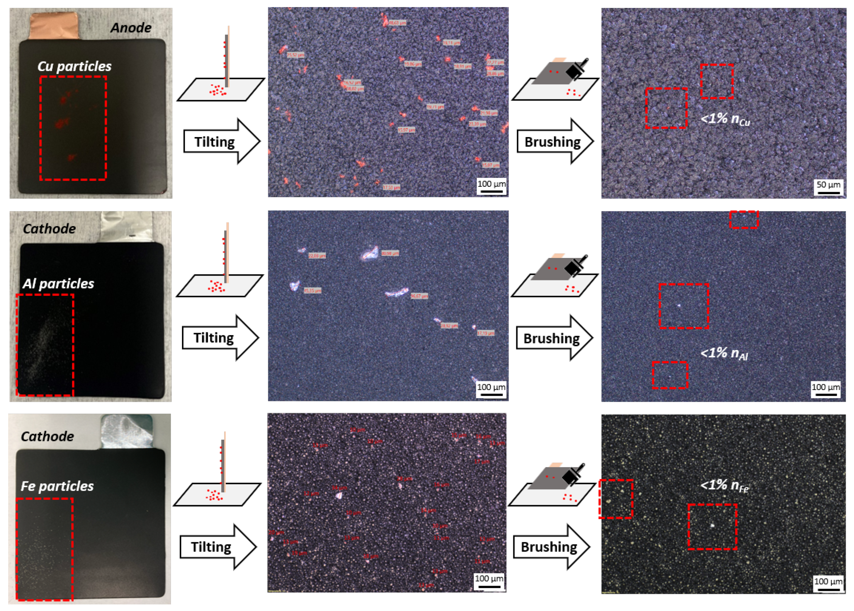
This appendix provides photographs and SEM images of all investigated contamination types, including Cu-contaminated anodes as well as Al- and Fe-contaminated cathode samples.
Figure A1.
Preparation of electrodes contaminated with Cu on the anode and with Al and Fe powders on the cathode. Photograph of particle distribution after scattering (left) and microscopy images of particle distribution after tilting (middle) and after cleaning by brushing (right).
Appendix B. Handling of Diffusion-Related Contributions in the DRT Analysis
As described in the main text, the diffusion-related contributions are handled by truncating the DRT at a high boundary. It should be explicitly noted that this approach is not recommended, if an accurate physical DRT of the system is required. However, that is not the objective of this work. The goal of this paper is the classification of different battery cells. The Warburg impedance may also contain information useful for classification. The problem is that DRT methods are unable to accurately represent Warburg-type contributions, in particular the Warburg-Open impedance. This becomes evident in Figure A2, which shows the full DRT without the truncation. The red curve represents the DRT obtained from the Gold algorithm, the blue curve shows the DRT that would result from a full equivalent circuit model (ECM) fit, and the green curve isolates the Warburg contribution from the same ECM fit. Given known parameters, both the impedance and the DRT of the Warburg-Open element can be computed analytically:
with
It must be noted that in practice these parameters are unknown. Whether the ECM fit correctly captures the true parameters cannot be verified. That said, Figure A2 clearly shows two important effects. First, the Warburg contribution overlaps with and distorts the peaks of the polarization processes. Second, artifacts can arise at the boundaries of the -range since the DRT cannot be evaluated as . To prevent these boundary values from disproportionately influencing the machine learning model, for example through overfitting to the last few DRT points, the extreme endpoints were truncated.
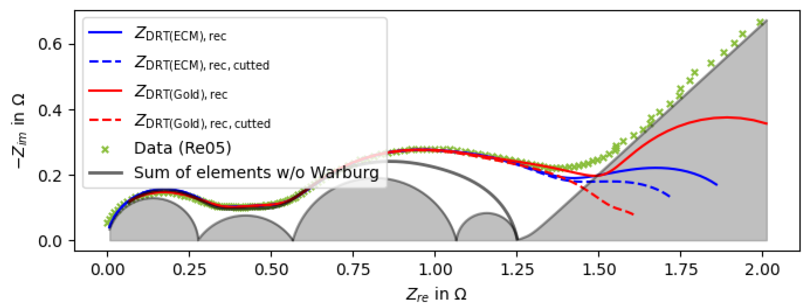
This truncation affects the impedance reconstruction. Due to the finite -range, poor reconstruction quality near the boundaries is expected even for well-fitted parameters, as a proper reconstruction would require extrapolation in the time domain. The DRTs with and without truncation from Figure A2 were used for impedance reconstruction in Figure A3.
Figure A2.
DRT spectra of a representative cell computed by the Gold algorithm and the full ECM fit. Additionally the Warburg contribution was isolated from the ECM fit and presented separately. The grey vertical line indicates the boundary used for truncating the DRT.
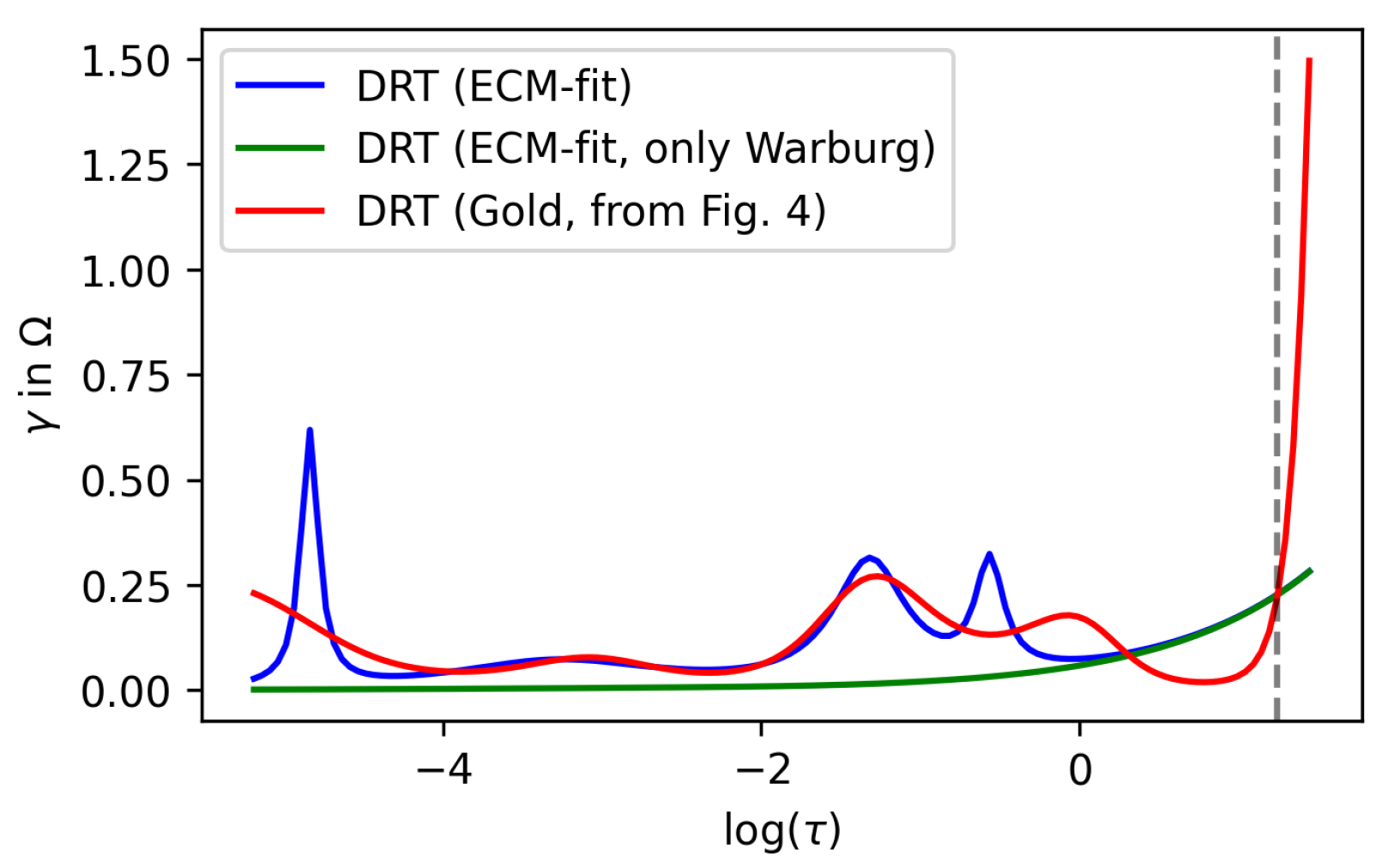
Figure A3.
Impedance spectrum of a representative cell reconstructed from the full and truncated DRT of the Gold algorithm and the full and truncated DRT of the ECM fit.
To summarize why this approach was chosen: the primary goal was to keep the data as unmodified as possible while removing boundary values that are prone to measurement noise. A physically more correct approach would involve fitting and subtracting the Warburg contribution for each cell individually. However, this would introduce an additional source of error through the fitting procedure, which could bias the machine learning model. Furthermore, the Warburg impedance may contain information that is relevant for classification and could be lost upon subtraction. For these reasons, a truncated DRT was chosen as a reproducible and consistent input for the machine learning algorithm. It should be acknowledged though that a DRT without Warburg subtraction is not physically rigorous, as the diffusion contribution overlaps with the polarization peaks and does not allow for an unambiguous physical interpretation of the DRT spectrum.
Appendix C. DRT Spectra for Different Regularization Parameters
As explained in Section 2.1, a regularization parameter that is too small leads to underfitting, while a value that is too large causes overfitting. Figure A4, Figure A5 and Figure A6 show all DRTs for increasing values of . It is evident that, for small , important features of the DRT are smoothed out and lost. In contrast, excessively large values cause the solution to be overly sensitive to noise, leading to pronounced oscillatory behavior. This behavior impairs the accuracy and reproducibility of the results of the machine learning program.
Figure A4.
All DRTs calculated with .
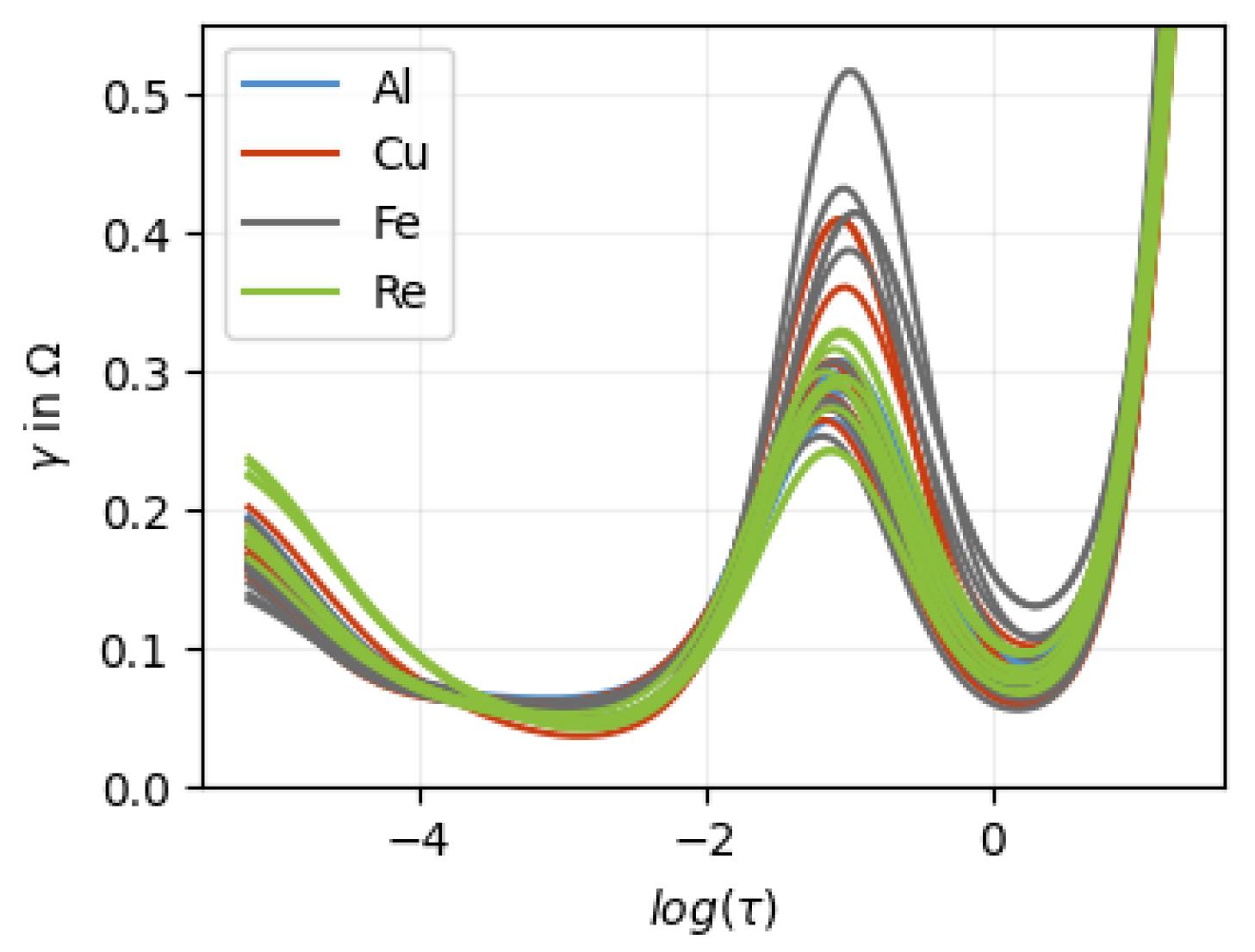
Figure A5.
All DRTs calculated with .
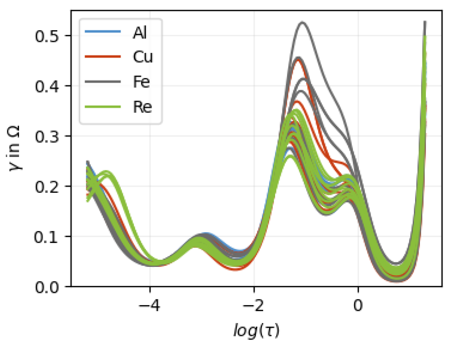
Figure A6.
All DRTs calculated with .
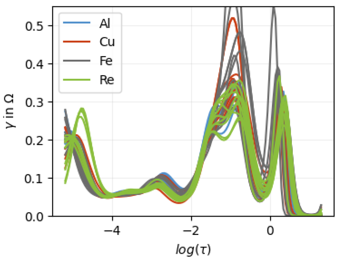
Appendix D. Computational Details
The best model performance was achieved using the following computational setup. PCA was performed using np.linalg.svd. For dimensionality reduction, the first SVD axes were used for classification. The DRT regularization parameter was set to ≈ 15,000.
All features were standardized using StandardScaler, fitted on the training data only in each cross-validation split to avoid data leakage. The classifier was implemented using MLPClassifier from scikit-learn. The optimal hyperparameters were:
- solver = “lbfgs”;
- hidden_layer_sizes = (30, 30, 30);
- activation = “relu”;
- max_iter = 10,000;
- max_fun = 15,000;
- alpha = 0.918.
All hyperparameters were varied during tuning, with a particular focus on (Figure 7). Hyperparameters were optimized using repeated cross-validation as described in the main text. The following software versions were used: Python 3.9.13, NumPy 1.26.4, Jupyter Notebook 7.1.1, and scikit-learn 1.4.1.
In addition, several feature engineering approaches were evaluated, including the frequency and value of the maximum as well as the integral of the DRT. These features did not lead to a measurable improvement in predictive performance.
Appendix E. ROC Graph
The ROC (Receiver Operating Characteristic) graph is a visual tool used to evaluate how accurately a model separates two groups. The curve starts at the bottom-left, identifying every data point to one group and ends at the top-right identifying every data point to the other group. The closer the curve reaches toward the top-left corner, the better the model performs. This perfect point represents 100% accuracy identifying everyone in one group correctly without mislabeling anyone from the other group.
Figure A7.
The ROC curves of both bar plots (Figure 4). The blue diagonal line represents the reference line corresponding to a random classifier.
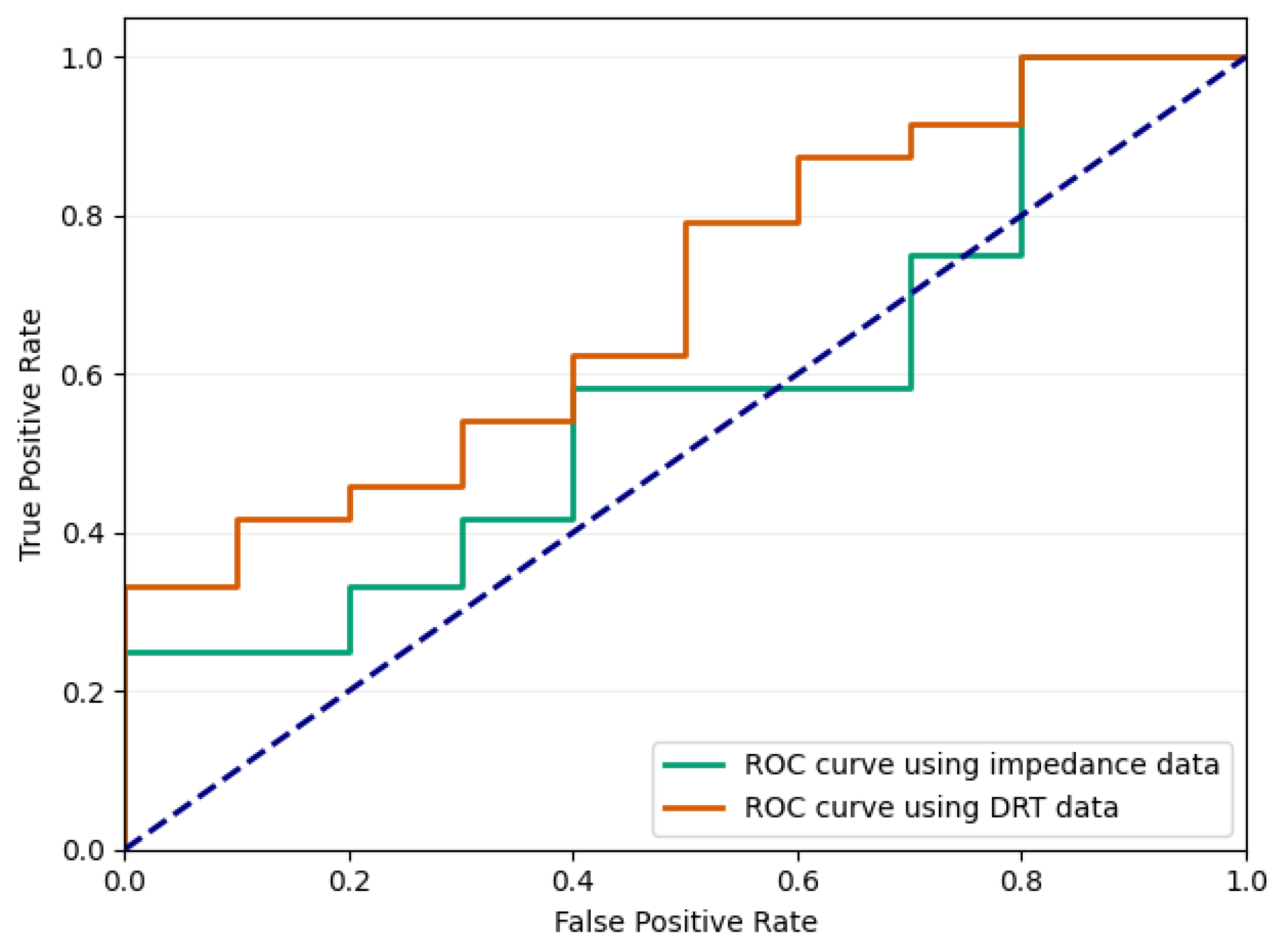
Both curves stay close to the diagonal, indicating that neither model can reliably separate the defective cells from defect-free cells. However, the DRT approach demonstrates marginal improvement.
Appendix F. Different Algorithm
A wide range of different parameter combinations and models were explored. However, only a selected subset of particularly relevant results is presented here. The best validation accuracies and corresponding standard deviations for the investigated classifiers are summarized in Table A1. The validation accuracies were obtained from 100 independent repetitions of 3-fold cross-validation. For each repetition, the mean accuracy over the three folds was calculated first. The validation accuracy and standard deviation were then calculated from these 100 mean accuracy values.
Table A1.
Comparison of best validation accuracy for different classifiers (MLP with ReLU and tanh activation, gradient boosting, and SVM).
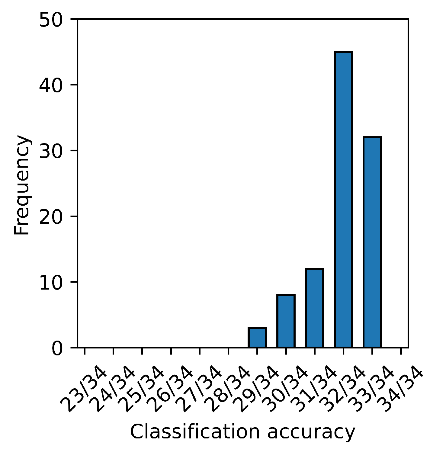
In addition, the distribution of the validation accuracies obtained from the 100 repetitions is illustrated as a histogram for each algorithm. In each repetition of the 3-fold cross-validation, every cell was used once as part of the validation dataset. The validation accuracy of one repetition is presented as the number of correctly classified validation cells divided by the total number of cells. Thus, each value in the histogram represents the accuracy obtained from one complete 3-fold cross-validation run. The histogram for the MLP classifier with ReLU activation is shown in Figure A8.
Figure A8.
Distribution of validation accuracies obtained from 100 independent 3-fold cross-validation using an MLP classifier with ReLU activation for .
Appendix F.1. Conclusion on MLP Classifier with Tanh Activation Function
The performance of the MLP classifier with a tanh activation function was nearly identical to that of the model using the ReLU activation. No significant differences in predictive performance or generalization ability were observed between the two configurations.
Interestingly, the optimal regularization parameter was found to be the same in both cases, indicating that the choice of activation function did not substantially influence the model’s sensitivity to regularization in this setting.
Best parameters for the MLP classifier with tanh activation:
- solver = “lbfgs”;
- hidden_layer_sizes = (30, 30, 30);
- activation = “tanh”;
- max_iter = 10,000;
- max_fun = 15,000;
- alpha = 0.918.
In Figure A9, the regularization parameter was varied.
Appendix F.2. Conclusion on Gradient Boosting
Compared to the other evaluated methods, gradient boosting did not perform well in this case. Despite extensive hyperparameter tuning, its overall performance remained inferior to the alternative models.
A key issue was its strong tendency to overfit: the model consistently achieved very high training scores, while validation performance was significantly lower. This indicates that gradient boosting quickly captures not only underlying patterns but also noise in the data, which negatively affects generalization.
Overall, gradient boosting proved to be less robust in this application and was unable to compete with the better generalizing methods.
Best Parameter for gradient boosting:
- n_estimators = 211 (= );
- learning_rate = 0.05;
- max_depth = 3;
- min_weight_fraction_leaf = 0.02;
- subsample = 0.7;
- min_samples_split = 5;
- min_samples_leaf = 2;
- max_features = log2.
In Figure A10, the number of estimators was varied.
Appendix F.3. Conclusion on SVM
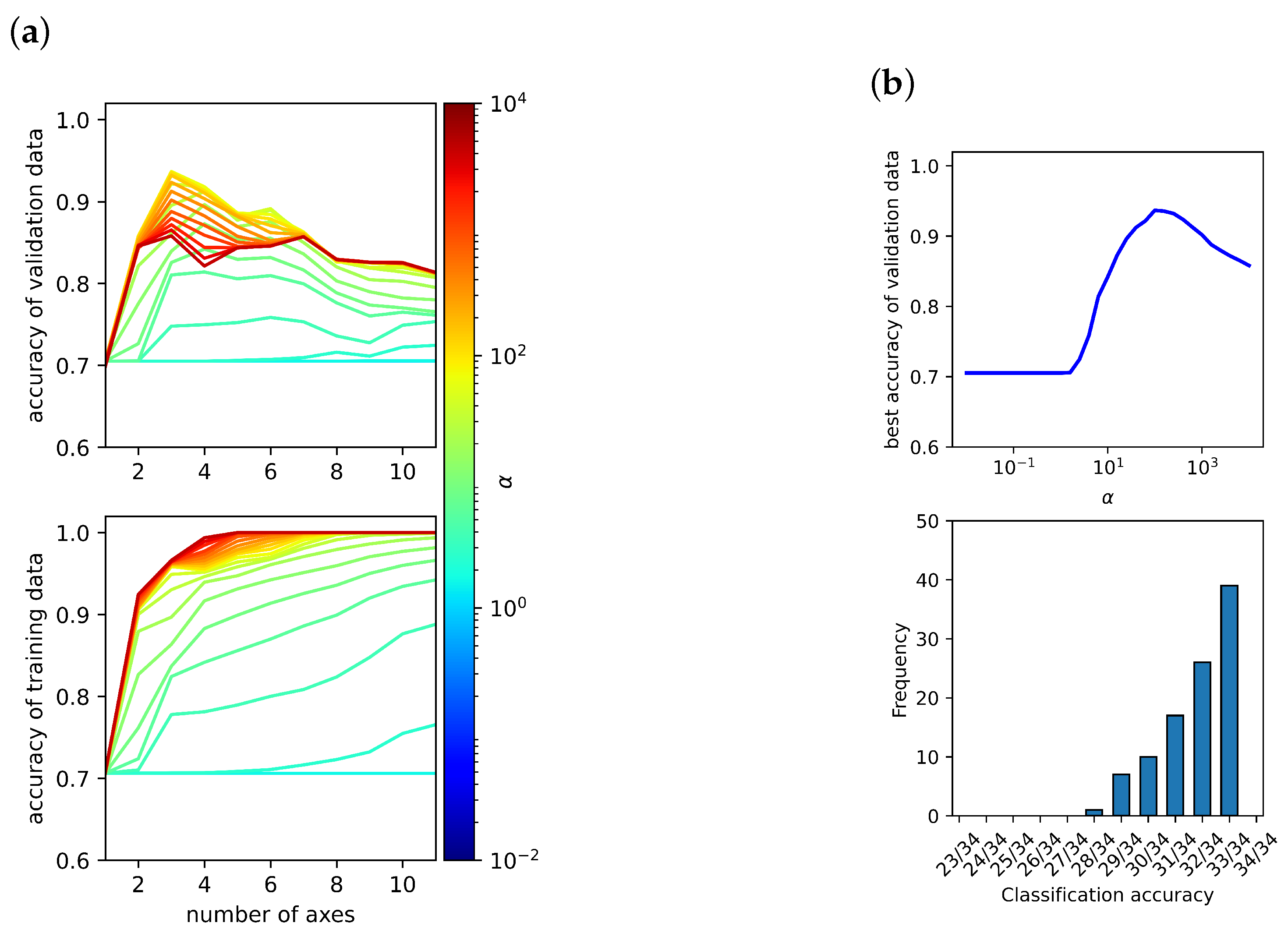
The SVM achieves performance comparable to the MLP classifiers, but remains slightly inferior overall. The model is primarily controlled by two hyperparameters, C and , which jointly determine the trade-off between model complexity and generalization.
For the selected value of , the model was not able to achieve perfect training accuracy when using three axes, indicating that the decision boundary remains too smooth to fully capture the structure of the training data. This suggests a limitation in model flexibility. Although both C and were systematically varied, no parameter combination was found that outperformed the MLP models.
The best parameters for the SVM are:
- kernel = “rbf”;
- C = 100 (= );
- gamma = 0.00794.
In Figure A11, the parameter C was varied.
Figure A9.
(a) The highest achievable accuracy for the validation and training data using a Neuronal-Network with a tanh activation function is plotted against the number of axes n and regularization parameter . (b) The upper plot shows the best validation accuracy for each , and the lower plot shows the distribution of the accuracies obtained from 100 independent 3-fold cross-validations for the best .
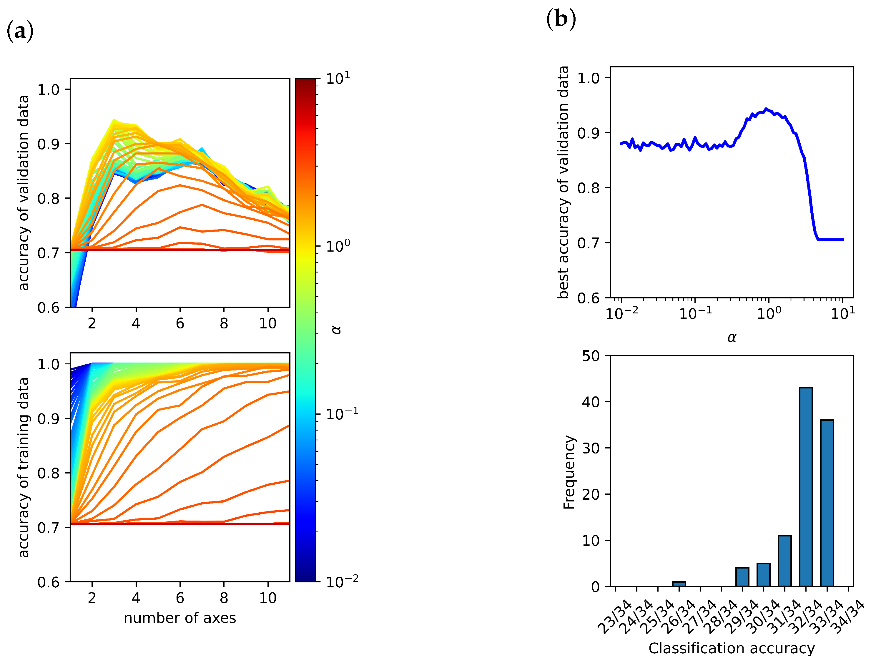
Figure A10.
(a) The highest achievable accuracy for the validation and training data using gradient boosting is plotted against the number of axes n and regularization parameter . (b) The upper plot shows the best validation accuracy for each , and the lower plot shows the distribution of the accuracies obtained from 100 independent 3-fold cross-validations for the best . Here, n_estimators.
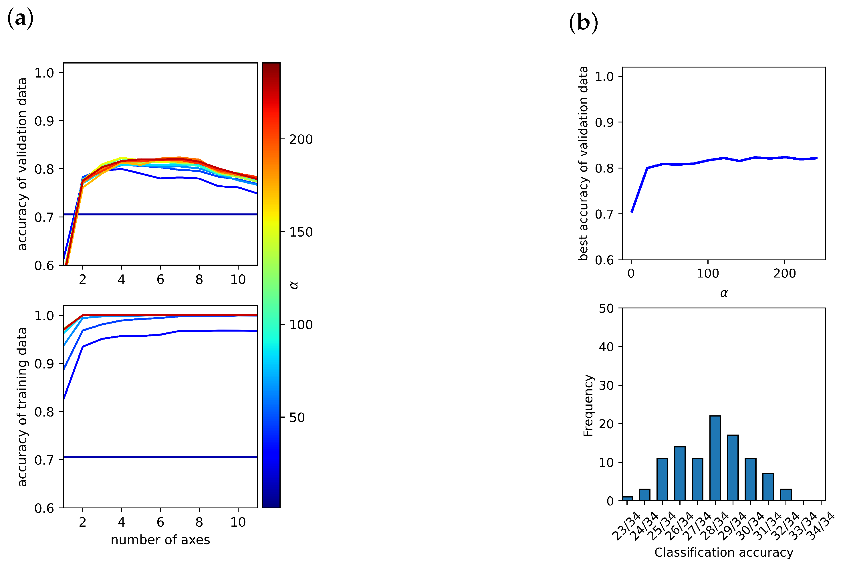
Figure A11.
(a) The highest achievable accuracy for the validation and training data using a support-vector-machine (SVM) is plotted against the number of axes n and regularization parameter . (b) The upper plot shows the best validation accuracy for each , and the lower plot shows the distribution of the accuracies obtained from 100 independent 3-fold cross-validations for the best . Here, in scikit-learn.
References
- Grabow, J.; Klink, J.; Benger, R.; Hauer, I.; Beck, H.P. Particle Contamination in Commercial Lithium-Ion Cells—Risk Assessment with Focus on Internal Short Circuits and Replication by Currently Discussed Trigger Methods. Batteries 2023, 9, 9. [Google Scholar] [CrossRef] [Scilit]
- Chen, W.; Han, X.; Pan, Y.; Yuan, Y.; Kong, X.; Liu, L.; Sun, Y.; Shen, W.; Xiong, R. Defects in lithium-ion batteries: From origins to safety risks. Green Energy Intell. Transp. 2025, 4, 100235. [Google Scholar] [CrossRef] [Scilit]
- Qian, G.; Monaco, F.; Meng, D.; Lee, S.J.; Zan, G.; Li, J.; Karpov, D.; Gul, S.; Vine, D.; Stripe, B.; et al. The role of structural defects in commercial lithium-ion batteries. Cell Rep. Phys. Sci. 2021, 2, 100554. [Google Scholar] [CrossRef] [Scilit]
- Sun, P.; Bisschop, R.; Niu, H.; Huang, X. A Review of Battery Fires in Electric Vehicles; Springer: New York, NY, USA, 2020; Volume 56, pp. 1361–1410. [Google Scholar] [CrossRef] [Scilit]
- Kurfer, J.; Westermeier, M.; Tammer, C.; Reinhart, G. Production of large-area lithium-ion cells - Preconditioning, cell stacking and quality assurance. CIRP Ann. Manuf. Technol. 2012, 61, 1–4. [Google Scholar] [CrossRef] [Scilit]
- Kim, M.; Jeon, Y.; Cho, Y.G.; Song, H.K. Nanobead-reinforced outmost shell of solid-electrolyte interphase layers for suppressing dendritic growth of lithium metal. J. Power Sources 2019, 414, 218–224. [Google Scholar] [CrossRef] [Scilit]
- Shinohara, K.; Furiki, M.; Seki, Y. Inspection and Analysis Solution for Quality Management of Lithium-ion Rechargeable Batteries. Hitachi Rev. 2022, 71, 482–486. [Google Scholar]
- Bakenhaster, S.T.; Dewald, H.D. Electrochemical impedance spectroscopy and battery systems: Past work, current research, and future opportunities. J. Appl. Electrochem. 2025, 55, 1657–1681. [Google Scholar] [CrossRef] [Scilit]
- Zhu, J.G.; Sun, Z.C.; Wei, X.Z.; Dai, H.F. A new electrochemical impedance spectroscopy model of a high-power lithium-ion battery. RSC Adv. 2014, 4, 29988–29998. [Google Scholar] [CrossRef] [Scilit]
- Xiao, F.; Xing, B.; Kong, L.; Xia, Y. Impedance-based diagnosis of internal mechanical damage for large-format lithium-ion batteries. Energy 2021, 230, 120855. [Google Scholar] [CrossRef] [Scilit]
- Protsenko, V.S.; Bobrova, L.S.; Butyrina, T.E.; Danilov, F.I. Hydrogen evolution reaction on Cr–C electrocatalysts electrodeposited from a choline chloride based trivalent chromium plating bath. Issues Chem. Chem. Technol. 2019, 61–66. [Google Scholar] [CrossRef] [Scilit]
- Wang, Z.; Li, J.; Wang, Y.; Wang, Z. An EIS analysis on corrosion resistance of anti-abrasion coating. Surf. Interfaces 2017, 6, 33–39. [Google Scholar] [CrossRef] [Scilit]
- Lee, Y.S.; Ryu, K.S. Study of the lithium diffusion properties and high rate performance of TiNb6O17 as an anode in lithium secondary battery. Sci. Rep. 2017, 7, 16617. [Google Scholar] [CrossRef] [Scilit] [PubMed]
- Mortadi, A.; El Hafidi, E.; Nasrellah, H.; Mghaiouini, R.; Chahid, E.; Monkade, M.; El moznine, R. Assessing the efficacy of polyaluminium chlorides in improving pool water quality using impedance spectroscopy. Results Eng. 2024, 21, 101911. [Google Scholar] [CrossRef] [Scilit]
- Susloparova, A.; Koppenhöfer, D.; Vu, X.T.; Weil, M.; Ingebrandt, S. Impedance spectroscopy with field-effect transistor arrays for the analysis of anti-cancer drug action on individual cells. Biosens. Bioelectron. 2013, 40, 50–56. [Google Scholar] [CrossRef] [Scilit] [PubMed]
- Brett, C.M. Electrochemical Impedance Spectroscopy in the Characterisation and Application of Modified Electrodes for Electrochemical Sensors and Biosensors. Molecules 2022, 27, 1497. [Google Scholar] [CrossRef] [Scilit] [PubMed]
- Randviir, E.P.; Banks, C.E. A review of electrochemical impedance spectroscopy for bioanalytical sensors. Anal. Methods 2022, 14, 4602–4624. [Google Scholar] [CrossRef] [Scilit] [PubMed]
- Wu, L.; Ogawa, Y.; Tagawa, A. Electrical impedance spectroscopy analysis of eggplant pulp and effects of drying and freezing-thawing treatments on its impedance characteristics. J. Food Eng. 2008, 87, 274–280. [Google Scholar] [CrossRef] [Scilit]
- Heins, T.P.; Leithoff, R.; Schlüter, N.; Schröder, U.; Dröder, K. Impedance Spectroscopic Investigation of the Impact of Erroneous Cell Assembly on the Aging of Lithium-Ion Batteries. Energy Technol. 2020, 8, 1900288. [Google Scholar] [CrossRef] [Scilit]
- Nakamura, T.; Homma, K.; Tachibana, K. Impedance spectroscopy of manganite films prepared by metalorganic chemical vapor deposition. J. Nanosci. Nanotechnol. 2011, 11, 8408–8411. [Google Scholar] [CrossRef] [Scilit] [PubMed]
- Vivier, V.; Orazem, M.E. Impedance Analysis of Electrochemical Systems. Chem. Rev. 2022, 122, 11131–11168. [Google Scholar] [CrossRef] [Scilit] [PubMed]
- Sgura, I.; Bozzini, B. Numerical issues related to the modelling of electrochemical impedance data by non-linear least-squares. Int. J. Non-Linear Mech. 2005, 40, 557–570. [Google Scholar] [CrossRef] [Scilit]
- Harrington, D.A.; Van Den Driessche, P. Mechanism and equivalent circuits in electrochemical impedance spectroscopy. Electrochim. Acta 2011, 56, 8005–8013. [Google Scholar] [CrossRef] [Scilit]
- Ivers-tiffée, E.; Weber, A. Evaluation of electrochemical impedance spectra by the distribution of relaxation times. J. Ceram. Soc. Jpn. 2017, 125, 193–201. [Google Scholar] [CrossRef] [Scilit]
- Hopfield, J.J. Neural networks and physical systems with emergent collective computational abilities. Proc. Natl. Acad. Sci. USA 1982, 79, 2554–2558. [Google Scholar] [CrossRef] [Scilit] [PubMed]
- Ahmed, M.; Najmul Islam, A.K. Deep Learning: Hope or Hype. Ann. Data Sci. 2020, 7, 427–432. [Google Scholar] [CrossRef] [Scilit]
- Bhattacharya, S.; Maddikunta, P.K.R.; Meenakshisundaram, I.; Gadekallu, T.R.; Sharma, S.; Alkahtani, M.; Abidi, M.H. Deep neural networks based approach for battery life prediction. Comput. Mater. Contin. 2021, 69, 2599–2615. [Google Scholar] [CrossRef] [Scilit]
- Wang, J.; Zhao, R.; Huang, Q.A.; Wang, J.; Fu, Y.; Li, W.; Bai, Y.; Zhao, Y.; Li, X.; Zhang, J. High-efficient prediction of state of health for lithium-ion battery based on AC impedance feature tuned with Gaussian process regression. J. Power Sources 2023, 561, 232737. [Google Scholar] [CrossRef] [Scilit]
- Fei, Z.; Yang, F.; Tsui, K.L.; Li, L.; Zhang, Z. Early prediction of battery lifetime via a machine learning based framework. Energy 2021, 225, 120205. [Google Scholar] [CrossRef] [Scilit]
- Severson, K.A.; Attia, P.M.; Jin, N.; Perkins, N.; Jiang, B.; Yang, Z.; Chen, M.H.; Aykol, M.; Herring, P.K.; Fraggedakis, D.; et al. Data-driven prediction of battery cycle life before capacity degradation. Nat. Energy 2019, 4, 383–391. [Google Scholar] [CrossRef] [Scilit]
- Lu, Y.; Zhao, C.Z.; Huang, J.Q.; Zhang, Q. The timescale identification decoupling complicated kinetic processes in lithium batteries. Joule 2022, 6, 1172–1198. [Google Scholar] [CrossRef] [Scilit]
- Rüther, T.; Gosea, I.V.; Jahn, L.; Antoulas, A.C.; Danzer, M.A. Introducing the Loewner Method as a Data-Driven and Regularization-Free Approach for the Distribution of Relaxation Times Analysis of Lithium-Ion Batteries. Batteries 2023, 9, 132. [Google Scholar] [CrossRef] [Scilit]
- Bergmann, T.G.; Schlüter, N. Introducing Alternative Algorithms for the Determination of the Distribution of Relaxation Times. ChemPhysChem 2022, 23, e202200012. [Google Scholar] [CrossRef] [Scilit] [PubMed]
- Shlens, J. A Tutorial on Principal Component Analysis. arXiv 2014, arXiv:1404.1100. [Google Scholar] [CrossRef] [Scilit]
- Qi, Y.; Liu, J.; Feng, M.; Tantratian, K.; Chen, L.; Xiao, X.; Sachdev, A.K. From the Passivation Layer on Aluminum to Lithium Anode in Batteries. Metall. Mater. Trans. A 2025, 56, 429–438. [Google Scholar] [CrossRef] [Scilit]
- Nasser, O.A.; Petranikova, M. Review of Achieved Purities after Li-ion Batteries Hydrometallurgical Treatment and Impurities Effects on the Cathode Performance. Batteries 2021, 7, 60. [Google Scholar] [CrossRef] [Scilit]

Disclaimer/Publisher’s Note: The statements, opinions and data contained in all publications are solely those of the individual author(s) and contributor(s) and not of MDPI and/or the editor(s). MDPI and/or the editor(s) disclaim responsibility for any injury to people or property resulting from any ideas, methods, instructions or products referred to in the content. |
© 2026 by the authors. Licensee MDPI, Basel, Switzerland. This article is an open access article distributed under the terms and conditions of the Creative Commons Attribution (CC BY) license.