


Abstract
Estimating the state of charge (SoC) is a critical task for effective management of electric vehicle batteries. Simple machine learning methods (LR, KNN, etc.) often suffer from limited prediction accuracy, while deep learning approaches (LSTM, CNN, etc.) generally require high computational resources and behave as black-box models with limited explainability. To overcome these limitations, the present work proposes a SoC estimation approach based on the Light Gradient Boosting Machine (LightGBM). The proposed model provides a balanced trade-off between prediction accuracy and computational efficiency. Furthermore, feature engineering is performed to derive additional informative features, improving the model’s ability to learn driving conditions and battery dynamics. In addition, the study incorporates a seasonal analysis by evaluating the model under both summer and winter conditions, allowing the impact of environmental variations on SoC estimation performance to be investigated. Moreover, Explainable Artificial Intelligence (XAI) techniques are employed to interpret the model predictions. Evaluation on real-world on-road data demonstrated that the proposed model achieved substantial improvements in estimation performance compared to recent studies.
1. Introduction
In recent years, Electric Vehicles (EVs) have become a focus of research due to the depletion of fossil fuel resources and increasing environmental concerns. Compared with conventional internal combustion engine vehicles, EVs provide a more sustainable and cleaner transportation mode, contributing substantially to the reduction in air pollution and carbon dioxide emissions [1]. Lithium-ion batteries are frequently utilized as the primary energy storage technology in EVs due to their relatively low self-discharge characteristics, long cycle life, and high energy density. However, the performance, safety, and lifetime of these batteries strongly depend on the effectiveness of the battery management system (BMS). The BMS monitors essential battery parameters, including voltage, temperature, and current, while also ensuring safe operation by preventing abnormal conditions. Among the various parameters monitored by the BMS, the State of Charge (SoC) is considered one of the most essential indicators for evaluating the available energy within the battery pack [2].
The SoC represents the ratio of the remaining battery capacity to its nominal full capacity and plays a role like the fuel gauge in traditional vehicles. Accurate estimation of SoC is crucial for optimizing energy management, determining the driving range, and ensuring reliable vehicle operation. Moreover, precise SoC estimation helps prevent battery degradation caused by deep discharge or overcharging, thereby extending battery lifetime and enhancing the overall safety of EV systems. Nevertheless, battery SoC cannot be measured directly and must therefore be estimated from measurable variables such as current, temperature, and voltage. The complex and nonlinear characteristics of lithium-ion batteries and the influence of operating conditions make accurate battery SoC estimation a challenging task [3].
Recently, various approaches have been proposed to estimate SoC, which can be commonly categorized into three main groups: model-based methods, filter-based methods, and data-driven methods. Model-based approaches rely on electrochemical or equivalent circuit models to represent the internal dynamics of batteries. Although these methods provide valuable physical insights, they often require complex mathematical formulations and detailed knowledge of battery characteristics. Filter-based techniques, such as Kalman filter variants, are widely employed to improve estimation accuracy by combining system models with measurement data. Nevertheless, these methods still heavily depend on the precision of the underlying battery model and may suffer from increased computational complexity in practical applications [4]. Recently, Data-driven approaches have attracted increasing attention for battery SoC estimation. These methods aim to capture the relationship between measurable battery parameters and SoC directly from the dataset, without relying on detailed electrochemical models. By exploiting historical battery measurements, data-driven techniques can learn complex associations among variables such as voltage, current, temperature, and operational conditions. As a result, they have demonstrated promising performance in improving estimation accuracy and adaptability under varying driving scenarios [5].
Despite recent methodological breakthroughs in SoC estimation, several limitations still exist in the current literature. Some existing approaches rely on computationally intensive deep learning models, which may limit their applicability in real-time embedded systems typically used in battery management units. Although such models often provide high predictive accuracy, their complex architectures, long training times, and significant computational requirements make them less suitable for practical deployment in resource-constrained environments. On the other hand, simple linear regression models may exhibit reduced robustness when applied to real driving scenarios. In addition, several studies focus mainly on laboratory datasets collected under controlled experimental conditions rather than real-world driving data. Such datasets may not fully capture the dynamic operating conditions experienced by electric vehicles in everyday use. Furthermore, some studies do not adequately account for relevant features such as road gradients. Additionally, seasonal variations are often overlooked, even though they significantly influence battery electrochemical behavior and SoC estimation accuracy. Temperature fluctuations can affect battery voltage characteristics, internal resistance, and energy efficiency, which in turn impacts the reliability of estimation models.
Unlike many existing studies that focus primarily on model development, this study adopts a data-centric and methodological perspective, where the main contribution lies in the design of the overall pipeline rather than the selection of a specific algorithm.
Furthermore, unlike previous studies relying on laboratory-controlled datasets, this study addresses the inherent variability, noise, and complexity of real-world driving conditions, making the problem more challenging and the results more practically relevant. To address existing challenges, this study proposes a lightweight and accurate battery SoC estimation framework based on the Light Gradient Boosting Machine (LightGBM) algorithm. The proposed approach is designed to achieve a balanced trade-off between estimation accuracy and computational efficiency, making it suitable for practical battery management applications. It is important to emphasize that the contribution of this study does not stem from the use of LightGBM itself, but from how it is embedded within a carefully designed data-centric framework. The framework incorporates feature engineering techniques that capture information related to driving conditions and battery dynamics. The novelty of this work lies in the construction of domain-specific features that better represent real driving conditions, rather than relying solely on raw sensor measurements. In addition, explainability analysis using SHAP (SHapley Additive exPlanations) and visualizing decision trees are employed to provide insights into the relative contribution of input variables, allowing a clearer understanding of how different factors influence SoC estimation. Such interpretability is particularly valuable for improving the transparency and reliability of data-driven models in safety-critical applications such as EVs. Moreover, a seasonal analysis is conducted to evaluate the robustness of the proposed model under different environmental conditions, specifically summer and winter driving scenarios. Seasonal variability is explicitly incorporated into the modeling process, which is rarely addressed in existing SoC estimation studies. By explicitly examining seasonal effects, the work aims to provide a more comprehensive evaluation of battery SoC estimation performance under varying temperature conditions encountered in real-world (on-road) driving environments. To the best of our knowledge, existing studies do not jointly integrate real-world on-road data, domain-specific feature engineering, and explicit seasonal analysis within a unified and explainable framework for SoC estimation.
This study does not aim to propose a new machine learning algorithm. Instead, it focuses on developing a comprehensive evaluation framework for SoC estimation. It utilizes real-world driving data collected under varying seasonal conditions and incorporates explainability techniques to better understand model behavior. Therefore, the main contribution of this study is a unified data-centric framework that combines real-world data, feature engineering, seasonal analysis, and explainability, rather than proposing a new standalone model. The key contributions of this research can be outlined as follows.
- i.
- A comprehensive data-centric SoC estimation framework is proposed, integrating real-world on-road driving data with machine learning to address the limitations of laboratory-based studies and enhance practical applicability.
- ii.
- A domain-informed feature engineering strategy is developed to construct additional variables reflecting driving dynamics, energy consumption behavior, and vehicle operating conditions, going beyond conventional raw sensor inputs and enabling improved representation of real-world scenarios.
- iii.
- A seasonal analysis is explicitly incorporated into the SoC estimation process to investigate the impact of environmental conditions (e.g., summer and winter) on model performance, which is rarely addressed in existing studies.
- iv.
- An explainable artificial intelligence (XAI) framework is integrated using SHAP values and decision tree visualization to provide interpretability and reveal the contribution and importance of input features under real-world conditions, addressing the black-box limitation of many existing approaches.
- v.
- The proposed framework is validated on a large-scale real-world electric vehicle dataset containing more than one million records, providing a robust and statistically reliable evaluation under realistic driving conditions.
- vi.
- A comprehensive comparative analysis is performed against existing approaches on the same dataset, demonstrating the effectiveness of the proposed data-centric framework rather than improvements driven solely by model selection.
The following sections outline the structure of this paper. Section 2 reviews the related literature on battery SoC estimation methods. Section 3 presents the materials and methods, including the proposed approach. Section 4 starts with the dataset description, followed by feature engineering and feature selection. The experimental setup, encompassing hyperparameter tuning and sensitivity analysis, is then detailed. The section also presents the evaluation results, integrated with statistical tests and explainability analyses via SHAP and tree visualization. Section 5 compares the proposed method with recent state-of-the-art studies. Finally, Section 6 presents the conclusions drawn from the study and briefly discusses possible subsequent investigations for future research.
2. Related Work
Recent studies on SoC estimation for lithium-ion batteries can be commonly categorized into several groups, including deep learning-based, observer-based, model-based, filter-based, and data-driven approaches [1,2,3,4,5,6]. In addition, hybrid methods that combine multiple estimation paradigms have also been explored in the literature. Table 1 provides a comprehensive overview of recent studies [7,8,9,10,11,12,13,14,15,16,17,18,19,20,21,22,23,24,25,26,27,28,29,30,31,32,33,34,35,36] on SoC estimation, summarizing their methodologies, datasets, evaluation metrics, and key characteristics. The comparative analysis presented in this table highlights emerging trends and common practices in the field, offering a structured perspective on the current state of research.
Table 1.
Overview of recent studies on SoC estimation (NA: Not Available, A: Available).
Deep learning-based approaches have been utilized in prior studies for SoC estimation. Various Convolutional neural network (CNN) architectures [7,8] have been employed to capture battery behavior from input signals such as voltage (V), temperature (T), and current (I). Recurrent neural network variants, particularly Long Short-Term Memory (LSTM) models [9], have also been explored to model patterns in battery dynamics. Similarly, bidirectional LSTM-based models, such as TCN-BiLSTM [10] and CNN-BiLSTM-AM [11], have been applied for SoC estimation. Additionally, a Gated Recurrent Unit (GRU)-based model [12] had been introduced to handle variations and abrupt changes in battery signals. Transformer-based approaches [13,14] have also been adopted for modeling battery characteristics by also introducing attention mechanisms. Despite being used in prior studies, these approaches generally involve high computational complexity, long training times, and limited interpretability due to their black-box nature.
Model-based approaches have also been investigated for SoC estimation. In [15], a μ-analysis-based estimator grounded in control theory was proposed to estimate both battery SoC and State of Health (SoH). Observer-based methods have likewise been explored. For instance, ref. [16] introduced a sliding mode observer combined with a diffusion-enhanced equivalent circuit model. These approaches rely heavily on accurate battery modeling and parameter identification, which may limit their generalization across different battery types and operating conditions.
Adaptive filter-based methods represent another category of SoC estimation techniques. In [17], a particle swarm optimized approach was proposed that combines the Smooth Variable Structure Filter (SVSF) and the Extended Kalman Filter (EKF) for state of charge estimation under varying ambient temperatures and battery aging conditions. In [18], a QPSO-AUKF algorithm was performed, integrating Quantum-behaved Particle Swarm Optimization (QPSO) with an Adaptive Unscented Kalman Filter (UKF) and online parameter identification to adjust the filter parameters for improved estimation. In [19], an adaptive iterative square root central difference Kalman filter (AII-SRCDKF) was proposed, incorporating a local iterative algorithm to refine the estimation process. In [20], a generalized mixture maximum correlation-entropy criterion (GMMCC)-based adaptive EKF was introduced to address inaccurate initial conditions and non-Gaussian noise. In [21], the impact of nonlinear parameters on SoC estimation was analyzed by comparing EKF, UKF, and Particle Filter (PF). These methods generally require careful tuning of filter parameters and are sensitive to model assumptions, which may restrict their applicability across different battery systems and operational scenarios.
Hybrid approaches combining data-driven and adaptive filter-based techniques have been explored in several studies. For example, Sun et al. [22] proposed an LSTM model integrated with physical constraints, feature engineering, and EKF. Shao et al. [23] introduced a GRU model with a physical-loss-based design combined with a UKF for SoC estimation in parallel and series battery modules. A Support Vector Machine (SVM)-based model fused with filtering techniques (AEKF) [24] had also been investigated. A digital twin-based framework combining LSTM, KF, and Random Forest (RF) had been proposed in [25]. These hybrid approaches, while integrating complementary techniques, generally involve increased structural complexity and require careful tuning.
Data-driven methods can rely on machine learning (ML) techniques for SoC estimation, including Multilayer Perceptron (MLP) [26], SVM [27], Adaptive Neuro-Fuzzy Inference System (ANFIS) [28], and Neural Networks [27,29]. Tree-based approaches, including RF and Extra Trees (ET), using Electrochemical Impedance Spectroscopy (EIS) features provided additional insights into battery behavior [30]. Similarly, ref. [31] evaluated a feedforward neural network (FFNN) alongside other methods for SoC estimation. The study presented in ref. [32] provided a comparison of many machine learning methods, including LR, SVR, RF, XGBoost, ET, KNN, NN, CNN, and LSTM, for battery SoC estimation on a simulated Tesla S dataset.
A wide range of metrics has been utilized to evaluate the accuracy and robustness of SoC estimation methods. Standard error measures, such as Mean Absolute Error (MAE) and Root Mean Squared Error (RMSE), were commonly reported [33] to provide a basic assessment of prediction accuracy. Percentage-based and normalized metrics, including Normalized Mean Squared Error (NMSE), Relative Error (RE) [34], and Mean Absolute Percentage Error (MAPE), were used to provide scale-independent assessments. Some studies also included additional indicators, such as the coefficient of determination (R2) [35], Mean Squared Error (MSE) [36], Maximum Error (MaxE), and Mean Bias Error (MBE). Furthermore, more specialized metrics, including Mean Absolute Scaled Error (MASE) and Mean Error Percentage (MEP), have been used in certain works [9] to achieve a more comprehensive performance evaluation. In contrast to regression metrics, classification-based evaluations focused on accuracy measures [30]. Computational efficiency was often assessed in terms of training time and memory usage.
Despite significant progress, several limitations remain in the literature. Many studies [7,9,10,11,12,13,14,15,16,17,18,19,20,21,22,23,24,25,27,28,29,30,31,32,33,34,36] relied on laboratory-collected or simulated datasets, which did not directly include parameters measured from an actual EV during real-world driving as model inputs, such as velocity, motor torque, braking signals, air conditioning power, longitudinal acceleration, and road grade. These idealized datasets typically lack the noise, anomalies, and complex aging patterns inherent in on-road operations. This work distinguishes itself by using real-life on-road data, capturing the inherent nature of actual driving cycles and environmental disturbances. Additionally, some studies [10,11,34] focused on temperature variations rather than a comprehensive seasonal analysis, as conducted in the present work. Furthermore, deep learning–based models are usually associated with high computational cost, long training times, and limited interpretability. These limitations underscore the need for lightweight, interpretable, and real-world applicable SoC estimation approaches that consider both environmental and seasonal variations.
Hybrid approaches [29,34] can provide reasonable accuracy, yet they introduce additional structural complexity. Some studies employed optimization techniques such as PSO and GA; however, these methods increase computational overhead beyond the model training time. Similarly, digital twin frameworks [25] offer scalability but demand substantial resources.
Simple machine learning approaches may offer a favorable alternative but can struggle with nonlinear dynamics and generalization due to their algorithmic simplicity. Model-based and adaptive filter-based approaches provide physical and mathematical characteristics, yet they rely heavily on accurate modeling and lack an intelligent learning paradigm. Another key observation is that most studies do not consider seasonal variability. Although some works incorporate temperature effects, comprehensive seasonal analysis remains limited. Most studies used a restricted set of input features, typically only three variables (V, I, and T), even though SoC is influenced by many more factors. Additionally, many studies relied on laboratory or simulated datasets rather than using parameters directly collected from an actual EV under real-world driving conditions in authentic road and weather environments. Consequently, there is a clear need for battery SoC estimation methods that balance accuracy, efficiency, interpretability, and real-world applicability while incorporating environmental and seasonal variations. Our study aims to address these identified gaps.
3. Materials and Methods
3.1. Proposed Approach
The proposed approach aims to develop a SoC estimation model for electric vehicles using an efficient algorithm. The proposed model is formulated as an instantaneous regression model rather than a sequence-based or recursive estimation approach. Unlike methods such as recurrent neural networks, the model does not rely on previous SoC values or temporal dependencies. Each prediction is made independently using only the features available at the current time step. By integrating feature engineering and seasonal analysis, the methodology is designed to offer robust estimation performance under various environmental conditions. A general overview of the proposed framework is presented in Figure 1.
Figure 1.
Proposed pipeline for SoC estimation.
The framework consists of eight main stages: data acquisition, data pre-processing, feature engineering, feature selection, machine learning, evaluation, prediction, and seasonal analysis. The process starts with data acquisition, where raw data is obtained from the electric vehicle battery management system during real-world on-road operation. The raw data includes numerous measurements, which are categorized into four main groups: vehicle dynamics, battery parameters, HVAC system metrics, and environmental factors. These variables represent the main factors affecting energy consumption in EVs and, consequently, the battery SoC. In the subsequent step, data preprocessing is conducted to enhance the overall data quality and integrity. Here, missing values are addressed, and irregular or invalid measurement-related records are handled to obtain more reliable and consistent datasets. In the next phase, feature engineering is performed to derive more meaningful and representative features, which are generated through feature construction guided by domain-based logic. Next, the feature selection step (i.e., Mutual Information) is performed to determine the most relevant features that contribute to improving the accuracy of SoC estimation. Following these steps, the light gradient boosting machine algorithm is employed to build the predictive model, taking advantage of its efficiency and ability to capture complex nonlinear relationships. Here, the model is also refined by applying hyperparameter analysis to enhance the predictive accuracy and robustness. Subsequently, the model is evaluated using several performance metrics, including RMSE, RMSPE, NMSE, MAE, and MAPE, to assess its prediction accuracy. After that, the trained model is used to predict SoC values on unseen data. To ensure the interpretability of the results, XAI is integrated into the process, providing a clear understanding of the decisions of the model and the contribution of each feature to the SoC estimation. Finally, a seasonal analysis is conducted to consider the SoC estimation across varying environmental and temperature conditions.
The target variable SoC indicates the proportion of remaining energy in the battery relative to its nominal capacity. It can be expressed as follows:
where denotes the battery’s current capacity, and represents the nominal capacity specified by the manufacturer, corresponding to the maximum amount of charge that the battery can hold. Since SoC is not a directly measurable quantity and depends on complex processes, it may not be accurately determined through direct measurement. SoC estimation methods can be categorized into two groups: direct or indirect. The most well-known direct methods are the look-up techniques and the Coulomb Counting approach. Model-based, data-driven, and their hybrid approaches are examples of indirect methods [37]. The Coulomb Counting method is a technique for determining the battery’s SoC. This approach establishes a direct relationship between battery current and SoC as follows:
where
- : Initial State of Charge at time
- : State of Charge at time
- : Coulombic efficiency, which is the ratio of the effective charge stored or released during charging/discharging
- : Battery current at time
3.2. Methodological Framework
This study builds a SoC estimation model based on the light gradient boosting machine method. This method is an efficient and fast implementation of gradient boosting decision tree (GBDT) algorithms designed for large-scale ML tasks. Gradient boosting builds predictive models by combining weak estimators, in the form of decision trees, into an ensemble model. The method was designed to improve computational efficiency through several algorithmic optimizations while maintaining high prediction accuracy. The objective is to minimize a differentiable loss function by iteratively adding trees that correct the residual errors of the previous model. Let the training dataset be defined as
where represents the input feature vector with m attributes and denotes the corresponding target variable. In the context of this study, the target variable corresponds to the battery SoC. The input features include vehicle dynamics, environmental factors, heating/cooling system metrics, and battery measurements obtained from real-world EV driving data. The method builds the model by sequentially adding regression trees that minimize the loss function. It employs a leaf-wise tree-growth strategy and a histogram-based split finding method, which reduces computational cost and improves efficiency for large-scale datasets.
- Step 1: Additive Training and Objective Function
The method constructs the final prediction model as an additive ensemble of decision trees. Instead of training a single complex model, multiple weak learners are sequentially added to improve prediction accuracy. At iteration t, the model prediction is updated as:
where is the ensemble model after t iterations, is the previous model, and denotes the newly added regression tree. Each decision tree is trained to reduce the residual errors of the current model. The optimization process is formulated through the following objective function:
where represents the loss function, K denotes the number of trees, and is the regularization term controlling tree complexity. The regularization function is defined as
where T is the number of leaves in the tree, is the prediction value of the leaf j, penalizes additional leaves, and λ is the L2 regularization parameter. This regularization prevents overfitting by limiting tree complexity.
- Step 2: Second-Order Taylor Approximation
Direct optimization of the objective function is computationally expensive. To simplify the optimization, the method approximates the loss function utilizing a second-order Taylor expansion.
To simplify the optimization problem, the loss function is approximated around the current prediction :
where
is the first-order gradient and
is the second-order derivative (Hessian) of the loss function. The gradient indicates the direction of error reduction, while the Hessian provides curvature information of the loss function. Using both derivatives enables more accurate and stable optimization. This quadratic approximation allows efficient computation of optimal leaf weights and split points during tree construction.
- Step 3: Optimal Split Finding Using Histogram-Based Algorithm
Finding optimal split points is computationally expensive in traditional tree algorithms because every feature value must be evaluated. The method addresses this issue using a histogram-based approach that discretizes continuous features into B bins. Each bin stores aggregated gradient and Hessian statistics. Let and denote the sum of gradients and Hessians for bin j. The quality of a candidate split is evaluated using the gain function:
where and are the gradient sums of the right and left nodes, λ is the regularization parameter, and are the Hessian sums, and γ is the penalty applied for creating a new split. The split with the maximum gain is selected as the optimal split.
- Step 4: Leaf-Wise Tree Growth Strategy
Conventional gradient boosting algorithms grow trees in a level-wise manner, expanding all nodes at the same depth. While this produces balanced trees, it may lead to slower convergence. LightGBM instead uses a leaf-wise growth strategy that expands only the leaf with the highest gain. Let the split gain be defined as Equation (12). The leaf with the maximum gain is selected as
The selected leaf is then split into two child nodes. The procedure proceeds until stopping conditions, such as minimum leaf samples or maximum depth, are reached. This strategy allows the model to focus on regions of the feature space that contribute most to reducing the loss function.
Algorithm 1 summarizes all steps of the proposed LightGBM-based SoC estimation framework in a unified and simplified manner, integrating the core components of the method into a single procedure.
| Algorithm 1. Simplified LightGBM Procedure for SoC Estimation |
Inputs:
Final SoC estimation model Begin
|
4. Experimental Studies
4.1. Dataset Description
In this study, an open-access dataset published on the IEEE DataPort platform was used, containing detailed measurements of battery performance and vehicle operational behavior [38]. The dataset encompasses numerous operational parameters collected under real-world driving conditions from the BMW i3 electric vehicle. This model stands out in the compact electric vehicle segment due to its architecture, lightweight structural design, and energy-efficient performance. The vehicle is equipped with a 60 Ah lithium-ion battery pack. The data were recorded via the vehicle’s On-Board Diagnostics (OBD) port and Controller Area Network (CAN) bus.
The data consist of 70 trips recorded in the Munich area, including urban routes in Munich East and Munich North as well as several highway segments. The dataset is categorized into 38 winter and 32 summer trips. Across all driving cycles, the vehicle covered a total distance of approximately 1340 km, with an average trip duration of about 30 min. Data acquisition was conducted at a sampling rate of 10 Hz, resulting in a large-scale time-series repository containing 1,094,793 records.
The descriptions of the variables used in this study are provided in Table 2. These features are categorized into four main groups: vehicle dynamics, battery parameters, HVAC system metrics, and environmental factors. The vehicle dynamics category includes variables that represent the vehicle’s instantaneous motion state, such as velocity, motor torque, throttle position, the regenerative braking signal, and longitudinal acceleration. Battery parameters comprise key electrical and thermal measurements describing the behavior of the energy storage system, including battery voltage, battery current, battery temperature, and electrical power. In addition, variables related to the HVAC system, such as heating power consumption and cabin temperature sensor readings, provide important indicators of in-vehicle energy usage. Environmental factors, including ambient temperature and road grade, represent external conditions that may influence vehicle energy consumption and battery behavior. The target variable, SoC, represents the relative amount of remaining energy in the lithium-ion battery with respect to its nominal capacity.
Table 2.
Description of the features used in the proposed SoC estimation model.
Overall, the dataset provides a comprehensive real-world representation of electric vehicle operation. It is well-suited for capturing the interactions between environmental conditions, vehicle dynamics, battery behavior, and auxiliary heating loads. This makes it particularly suitable for research on battery state prediction.
Table 3 shows the descriptive statistics of all features utilized in the model development process. Specifically, the minimum, maximum, standard deviation, and mean are reported for each feature to illustrate the dataset’s distributional characteristics. For instance, vehicle velocity ranges from 0 to 152.26 km/h, with an average of 45.54 km/h. The battery-related parameters, such as voltage and current, span broad value ranges, reflecting diverse operating conditions of the electric vehicle. Similarly, the ambient temperature ranges from −3.5 °C to 33.5 °C, indicating that the dataset captures different environmental conditions. The target variable, SoC, ranges from 15.40% to 88.50%, indicating that the dataset spans a range of battery charge states across different operating scenarios. These statistical summaries provide an important basis for understanding the overall structure of the dataset and for determining appropriate data preprocessing steps during model development.
Table 3.
The descriptive statistics of features.
Table 4 presents a representative subset of data collected to illustrate its structure and variability. As shown in the table, the data include measurements obtained from different seasonal periods, specifically summer and winter driving conditions. Incorporating observations from multiple seasons is particularly important in electric vehicle studies, as environmental conditions and vehicle operating states can substantially influence battery behavior and energy consumption patterns. Seasonal variations in ambient temperature and HVAC system usage may lead to significant differences in battery load and thermal characteristics. For instance, the winter samples exhibit lower ambient temperature values and noticeable heating power consumption. In contrast, the summer samples generally show higher ambient temperatures and different energy consumption patterns, including cooling system usage. The inclusion of temporally diverse observations enables the dataset to capture a wide range of real-world operating conditions, thereby enhancing the robustness and generalization of the proposed SoC estimation model.
Table 4.
Sample records from the dataset.
Figure 2 presents a visualization of key features to examine the temporal behavior of the dataset’s variables. These plots provide an overview of how key variables evolve across different samples, and help illustrate the variability present in real-world electric vehicle operating conditions. The variables exhibit distinct temporal patterns reflecting variations in vehicle dynamics, battery behavior, and environmental conditions. Vehicle dynamics variables, such as velocity and motor torque, exhibit noticeable fluctuations during acceleration, cruising, and braking phases, while the regenerative braking signal (RBS) intermittently appears, indicating periods of braking activation.
Figure 2.
Temporal visualization of key dataset features (a) battery temperature, (b) road grade, (c) air conditioning power, (d) vehicle velocity, (e) ambient temperature, (f) regenerative braking signal (RBS), (g) cabin temperature, (h) battery voltage, (i) motor torque, and (j) state of charge (SoC).
Battery-related parameters also exhibit meaningful temporal changes: battery voltage fluctuates in response to varying power demand, whereas the SoC gradually decreases, with short-term oscillations typical of battery discharge during driving cycles. Environmental variables reveal clear seasonal characteristics within the dataset. In particular, the ambient temperature and cabin temperature plots show segments corresponding to summer and winter conditions, with higher temperature ranges representing summer periods and lower values indicating winter driving conditions. These seasonal differences are also reflected in HVAC-related variables: air conditioning power consumption increases during summer periods to meet cabin heating requirements, while colder periods exhibit different usage patterns. In the road grade figure, positive values correspond to uphill segments, whereas negative values indicate downhill driving conditions. The varying magnitudes reflect both mild and steep slopes, capturing diverse driving scenarios.
4.2. Data Preparation and Feature Engineering
Prior to model development, various preprocessing steps were carried out to ensure data consistency and quality. First, irrelevant attributes unrelated to the SoC estimation task were removed from the dataset. The raw data contained missing values and irregular entries resulting from sensor measurements and data-acquisition processes. In particular, records with missing SoC values were eliminated to avoid inconsistencies during model training. In addition, invalid measurements were filtered.
Following data cleaning, feature engineering was performed to enhance the representational capacity of the dataset and better capture the physical processes governing energy consumption in electric vehicles. One of the key derived features is road grade, which replaces the raw elevation variable. Although elevation provides absolute altitude information, it is solely insufficient for modeling energy consumption, as battery load is primarily influenced by elevation changes rather than absolute height. Therefore, the road grade was computed using time, velocity, and elevation measurements as given in Equation (13). In addition, several data-related factors that may affect SoC estimation reliability were considered. Since the dataset was collected from mounted EV sensors through the On-Board Diagnostics (OBD) port, it inherently reflects variations arising from sensor characteristics and operating conditions, including potential sensor noise. To ensure data quality, preprocessing steps such as the removal of invalid records and the handling of missing values were applied.
Furthermore, the dataset was examined in terms of distribution and consistency to mitigate potential data imbalance and ensure a balanced representation across different operating conditions. Battery aging effects are also inherently reflected in the dataset, as variations in battery characteristics over time are captured under real-world driving conditions. These considerations enhance the robustness and reliability of the proposed model.
This formulation captures the relative slope of the road, with positive values indicating uphill driving and negative values corresponding to downhill segments. By transforming elevation into grade, the feature effectively represents terrain variations from slight inclines to steep slopes, thereby incorporating diverse driving environments into the modeling process. This transformation is particularly important, as road grade directly influences potential energy variations and vehicle load dynamics, which are key factors affecting the vehicle’s energy demand and, consequently, the evolution of the battery SoC.
In addition to the existing features, a new variable, Power, was derived from battery voltage and current measurements. The power was computed as given in Equation (14).
This feature represents the instantaneous power flow of the battery system and provides a direct measure of the energy being drawn from or supplied to the battery during vehicle operation. Unlike voltage or current signals considered individually, power integrates both electrical dimensions into a single physically meaningful quantity, thereby offering a more informative and comprehensive representation of the battery’s operational state. From a physical perspective, power is directly related to the rate of energy consumption, making it highly relevant for modeling battery discharge dynamics. Variations in power reflect changes in driving conditions such as acceleration, deceleration, and auxiliary system usage, all of which influence the battery’s state of charge. Consequently, incorporating power as a derived feature enables the model to better capture the relationship between energy demand and SoC evolution.
After preprocessing and feature engineering, the final dataset was split into training and test sets at a 70–30 ratio. To maintain consistency with previous studies conducted on the same dataset and to enable a fair comparison, a random splitting strategy was adopted. Before splitting, the data were shuffled to reduce potential bias related to specific trips or time segments. In this study, the problem is formulated as a supervised regression task based on instantaneous features rather than a sequential forecasting problem. In addition, the model uses only information available at the current time step, without incorporating any future or lag-based variables that might introduce temporal leakage. This approach is consistent with prior studies and supports methodological comparability across studies. Furthermore, no sequential or lag-based features were constructed. The model does not explicitly learn temporal dependencies between consecutive observations. Although the dataset is derived from a time-dependent process, the modeling approach does not introduce temporal leakage. This is because each sample is constructed using only information available at the corresponding time step. In addition, the model is not exposed to any future observations during training or evaluation. Accordingly, 742,854 samples were allocated to the training set and 318,366 samples to the testing set. The test subset was further analyzed for seasonal evaluation, comprising 140,488 summer records and 177,878 winter records, enabling assessment of the proposed SoC estimation model across different environmental conditions.
To further evaluate the contribution of the engineered features, an additional experiment was conducted by excluding power and road grade from the input set, which resulted in a decrease in model performance, indicating that these features provide valuable information for SoC estimation. This observation is also supported by interpretability analyses. In the decision tree structure, power appears in upper-level splits, suggesting its strong influence on early decision-making, while SHAP analysis ranks power among the most important features (second-highest), confirming its significant contribution to model predictions. Similarly, road grade (slope) affects vehicle load, as the required traction force and battery power demand depend on the road’s inclination. These findings demonstrate that well-motivated feature transformations can enhance model performance.
4.3. Feature Selection
Feature selection is a significant phase in ML that involves selecting the features that contribute most to the prediction variable in order to improve model performance. Therefore, irrelevant features are removed to increase the model’s estimation accuracy. Compared to correlation-based methods such as Pearson correlation, which only capture linear relationships, MI can detect both linear and non-linear dependencies. Wrapper methods such as Recursive Feature Elimination (RFE), although powerful, are computationally expensive and model-dependent. Similarly, embedded methods may introduce model-specific bias. Considering the relatively small number of features and the selected model’s ability to handle feature interactions, MI was considered a suitable choice for this study. MI-based feature selection helps to identify the features with the greatest impact on the target variable, thereby enhancing the model’s interpretability and efficiency.
The steps for MI-based feature selection are as follows:
- First, MI scores are calculated between the features and the target variable. It is calculated as:
- In the next step, features are sorted based on their MI scores, and the top-ranked ones are retained. At this stage, a threshold value can be specified so that the features with the highest MI scores are preserved.
Figure 3 presents the mutual information (MI) scores of all 14 input features, shown in descending order to indicate their relative importance. A threshold of 0.4 was applied to retain the most informative features, resulting in the selection of 10 features for inclusion in the model. As illustrated in the figure, the CabinTemperatureSensor feature was specified as having the strongest relationship with the target variable, with an MI score of 1.90. This is followed by AmbientTemperature, BatteryVoltage, BatteryTemperature, and HeatingPowerCAN features, respectively. These results highlight the significance of seasonal variables on the model, emphasizing the necessity of conducting a seasonal analysis for accurate SoC estimation. On the other hand, some features, such as RegenerativeBrakingSignal, had low MI values. This suggests that these variables have a weak dependency on the target variable and may contribute only to limited model performance.
Figure 3.
Mutual information scores for the features, highlighting the most informative ones.
4.4. Evaluation Metrics
In predictive modeling and forecasting, selecting the right metric is crucial because each one penalizes errors differently. The Mean Absolute Error (MAE), Root Mean Squared Error (RMSE), Root Mean Squared Percentage Error (RMSPE), Mean Absolute Percentage Error (MAPE), and Normalized Mean Squared Error (NMSE) metrics were employed to ensure a fair comparison both among the models tested in this study and with existing research in the literature. Utilizing a diverse suite of metrics also facilitates a comprehensive assessment of model efficacy, capturing critical dimensions such as predictive precision and residual distribution.
MAE serves as a metric for the average absolute distance between the predicted SoC outputs and actual SoC data:
where is the number of samples, is the predicted SoC value by the prediction model, and is the actual SoC value in the test set. Since the error is not squared, the metric remains robust to outliers by preventing individual extreme values from disproportionately inflating the overall result.
RMSE evaluates the precision of SoC estimation by calculating the square root of the average squared discrepancies between the predicted and actual battery states. It intentionally penalizes significant predictive failures by squaring error terms, which increases its sensitivity to outliers. RMSE provides an interpretable measure of error by maintaining the same units as the original data:
RMSPE measures the average relative difference between actual and predicted values by calculating the square root of the average squared percentage errors. It is ideal for evaluating forecasting models where relative percentage differences are more meaningful than absolute error magnitudes:
MAPE measures the deviation of predictions from actual values as a percentage, providing an idea of how far off predictions are relative to the scale of the data:
NMSE normalizes the traditional Mean Squared Error (MSE) by the variance of the actual values. This provides a relative benchmark that remains invariant to the magnitude of the target variables. Consequently, it ensures comparability across different datasets and offers a more consistent measure of predictive precision than its non-normalized counterparts:
where is the mean of the SoC values. The smaller the error values obtained from the used evaluation metrics, the higher the model accuracy.
4.5. Results
All implementations in this work were performed using Python 3.14.3 and various libraries such as sklearn, pandas, numpy, and matplotlib. All experiments were carried out under the same configuration to ensure fair and consistent performance evaluation. They were conducted on a system equipped with a 1.9 GHz Intel Core i.7 processor and 8 GB RAM. To ensure reproducibility, a fixed random seed (specifically 42) was used in all experiments.
This study tested different machine learning algorithms for battery SoC estimation to evaluate their capability to generate precise temporal forecasts based on historical data. Such predictive accuracy is instrumental in refining electric vehicle control strategies and streamlining the integration of auxiliary components. To ensure peak performance, a grid search technique was initially employed to ascertain optimal hyperparameters. Table 5 shows the comparative performance of the evaluated models. The reported results represent the mean values obtained from 10 individual experimental trials for each model. The evaluation was conducted across distinct statistical metrics, alongside computational training time to provide an assessment of model efficacy.
Table 5.
Performances of the prediction models for SoC estimation.
The experimental results revealed that LightGBM outperformed other predictive models. In particular, it achieved the highest predictive fidelity, yielding the lowest errors across all metrics (MAE: 0.9117, RMSE: 1.2900, etc.). This means that the model is highly adept at capturing the non-linear dynamics of battery discharge cycles. Furthermore, its low NMSE value indicates that this model estimates the target value well, representing a substantial improvement over the baseline mean.
A critical observation was made by comparing the MAE and RMSE values across all models. For instance, in the Neural Network model, the RMSE is notably higher than the MAE (7.0723 vs. 5.1477, respectively). This discrepancy suggests the presence of occasional large residuals or outliers in the predictions, which the RMSE is sensitive to. In contrast, the narrow gap between these metrics in the LightGBM model confirms not only high average accuracy but also consistent error distribution and high reliability.
Simple traditional ML approaches, such as LR, KNN, and EN, demonstrated lower performance (MAE > 3.02) than LightGBM. This result suggests that conventional ML methods may have limited capacity to capture the nonlinear, complex relationships present in the dataset. The relative underperformance of the RF and ET models may be attributed to the specific nature of the dataset, which appears to favor the boosting and leaf-wise growth strategies of LightGBM over bagging-based methods.
From the perspective of on-board implementation in electric vehicles and large-scale datasets, computational overhead is a vital constraint. LightGBM offers a superior trade-off between precision and efficiency. While LR was the most computationally efficient, its error rates were higher than those of LightGBM, making LightGBM the most viable candidate for high-accuracy real-time SoC estimation.
Figure 4 illustrates the relationship between the predicted and actual battery SoC values obtained by the LightGBM model for the first 1400 records of the test data. A strong positive linear correlation was observed, with the values closely following the diagonal line. The figure indicates that the model achieves low error variance and high prediction accuracy.
Figure 4.
Results of the SOC estimation by LightGBM.
Figure 5 illustrates the fluctuation of error residuals over a sequence of 100 samples for the compared methods. LightGBM, the best-performing model, has error margins that are more concentrated around the zero baseline compared to the other models. This suggests that the underlying model is unbiased, as the residuals do not exhibit a systematic positive or negative offset. The model maintains constant variance across the dataset. The majority of the error values are tightly clustered within a narrow range. While there are occasional stochastic outliers, they remain well within an acceptable margin, indicating a high degree of precision in the estimations.
Figure 5.
Error between predicted and actual battery SoC values.
The histogram in Figure 6 shows the distribution of residuals (prediction errors) for the LightGBM model across the entire test set. The provided histogram and the statistical parameters μ = 0.001, = 1.29 and = 1.66 indicate that the residuals follow a near-normal distribution and the predictions are unbiased (visually symmetric around 0). The stochastic nature and Gaussian distribution of the residuals demonstrate that the model provides a high-quality fit to the dataset.
Figure 6.
Histogram of the error residuals across the entire test set.
Figure 7 shows the convergence characteristic of the LightGBM model. It illustrates the evolution of the MAE over 250 training iterations. The process demonstrates a high learning rate in the initial iterations, followed by a refined convergence beyond 50 iterations. The final MAE stabilizes at a negligible level, confirming the robustness of the proposed model and its ability to effectively minimize predictive bias. The smoothness of the curves implies an appropriately selected learning rate and a well-conditioned loss landscape, preventing the model from overshooting local minima.
Figure 7.
Training convergence curve.
A non-parametric statistical analysis was conducted to evaluate the relative effectiveness of the tested models. The Quade Test was performed to assess the performance differences across the evaluated methods. The results yielded a p-value of 0.00347, leading to the rejection of the null hypothesis at a 0.05 confidence level. This indicates a statistically significant difference between the experimental groups.
4.6. Explainable AI Analysis for the Proposed Model
Figure 8 illustrates the global feature importance and the directional impact of each input variable on the model’s output using SHAP. The SHAP summary plot helps explain how the predictive model works by addressing the black-box issue in complex models, providing transparency and improving trust. BatteryVoltage stood out as the most important feature, showing a strong positive relationship with the target variable. High feature values (red) are densely clustered on the positive side of the SHAP axis, indicating that higher voltage is the most significant driver of increased model predictions. In contrast, Power and BatteryTemperature variables have a negative correlation with the target variable. Velocity shows a positive correlation, suggesting that as the vehicle speed increases, the model output increases accordingly. While most BatteryCurrent values have a neutral impact, high current peaks significantly penalize the model output. The remaining attributes exhibit a vertical distribution centered around the zero-line, indicating localized influence on the target variable. The generated features, Power and Road Grade, are among the top ten features, with Power notably ranking second. Conversely, aside from velocity, no other features within the vehicle dynamics category made this list. This analysis underscores the significant impact of the generated features on the model’s predictive performance.
Figure 8.
Explainability analysis of the proposed model, (a) SHAP values obtained for features, (b) Feature importance ranking according to SHAP analysis.
The dominance of the identified features in the SHAP analysis stems from the fundamental electrochemical processes of Lithium-ion batteries. According to the Nernst Equation, the open-circuit voltage (OCV) has a direct logarithmic relationship with the lithium-ion concentration at the electrodes. Power serves as a proxy for the discharge intensity. High power demands lead to significant polarization effects. These effects cause the terminal voltage to deviate from the OCV. By prioritizing Power, the model effectively compensates for these nonlinear voltage drops, which are critical for maintaining SOC accuracy during aggressive driving maneuvers. Temperature dictates the kinetics of electrochemical reactions and the diffusivity of lithium ions in both the electrolyte and the solid electrode phases. At lower temperatures, internal resistance increases due to reduced ionic conductivity, while higher temperatures may accelerate side reactions. Observed feature prioritization aligns with the Butler-Volmer equation and Fick’s laws of diffusion, in which voltage, current, and temperature govern the internal state transitions of the battery cells [39].
It is important to note that feature rankings obtained from MI and SHAP analysis can be distinct because of their different approaches. MI is a model-independent, filter-based technique that evaluates the statistical dependence between each feature and the target variable in isolation, ignoring interactions among features. On the other hand, SHAP analysis is model-specific and measures the actual impact of each feature on the model’s output by considering nonlinear correlations and interactions between features. Consequently, a feature like BatteryVoltage, which SHAP identified as the most influential, reflects its dominant role in the model’s internal decision-making process, whereas a feature like CabinTemperatureSensor, which has a high MI score, indicates a strong individual relationship with the target variable. Therefore, features with high MI scores may not necessarily appear as the most influential in SHAP analysis, and these methods provide complementary insights rather than conflicting results.
Figure 9 presents a representative decision tree to better illustrate the decision-making process of the proposed model. This tree shows the relationships between the features used to estimate the Battery State of Charge (SoC) in electric vehicles. The split condition BatteryVoltage ≤ 377.49 at the root node of the tree shows that battery voltage is regarded by the model as one of the most informative features for predicting SoC. After this separation, the model creates different decision paths using features such as power and velocity. While electrical parameters such as battery voltage and power consumption play an important role at the upper levels of the tree, environmental and thermal features such as ambient temperature, battery temperature, and cabin temperature become more influential at the next levels. This can be explained as follows: first, the vehicle usage scenario is determined, and then the prediction is adjusted according to environmental and thermal conditions. In some branches, for instance, after the condition BatteryVoltage ≤ 373.00 is satisfied, the model refines the decision process according to battery current thresholds.
Figure 9.
Visualization of the decision tree used for SoC estimation.
In the tree, the leaf value does not directly represent the predicted SoC, but rather the contribution of that leaf to the overall prediction in the additive ensemble model. The count values in the leaf nodes indicate how many samples follow each decision path, reflecting which conditions appear more frequently in the dataset. For example, some leaves have very high numbers, such as the count value of 34,009 in leaf 19. This indicates that the model is learning specific situations frequently within the data.
Overall, this decision tree clearly demonstrates how the model evaluates multidimensional sensor data in SoC estimation. In particular, considering the variables of battery voltage, power consumption, velocity, battery current, and temperatures together enables the model to evaluate battery behavior under different operational and environmental conditions.
The structure of the decision tree can also be interpreted in terms of the physical behavior of the battery system. Since voltage is one of the primary indicators of the battery’s charge condition, the appearance of BatteryVoltage at the root node shows its direct electrochemical relationship with SoC. At the upper levels of the tree, features such as Power and BatteryCurrent appear, which are closely related to load conditions and charge dynamics. These variables indicate how much energy the vehicle is using and how current flows, both of which affect voltage fluctuations and effective SoC estimation under real driving conditions.
As the tree goes to lower levels, temperature-related features (AmbientTemperature, BatteryTemperature, and CabinTemperature) become more prominent. This hierarchical transition is consistent with battery system dynamics, where thermal conditions affect internal resistance, efficiency, and energy losses, thereby refining the SoC estimation.
Additionally, the tree’s shallow depth indicates that the model captures dominant relationships without excessive complexity, leading to low computational costs and making it suitable for real-time applications.
4.7. Hyperparameter Tuning
Choosing appropriate hyperparameters is essential, as poor configurations can cause the model to either underfit or overfit the training data. To identify the best setting for each model, an exhaustive Grid Search was carried out. To ensure a fair and consistent comparison among all evaluated models, the same hyperparameter optimization strategy was systematically applied across all algorithms. For each model, a predefined search space was defined based on commonly used parameter ranges in the literature. Preliminary experiments were also conducted to identify stable and effective configurations. All candidate configurations were evaluated under identical experimental conditions. This ensures that all models were subject to the same level of optimization effort. The models under investigation fall into five categories based on their learning strategy: instance-based methods, linear models, neural networks, bagging ensembles, and boosting ensembles. Table 6 presents the complete search configuration, along with the optimal values found through Grid Search. In addition, all models were trained and evaluated using the same training–testing split. A consistent preprocessing pipeline was applied to reduce potential bias arising from differences in data handling. This unified experimental setup ensures that performance differences can be attributed to the learning capabilities of the models rather than inconsistencies in the evaluation procedure.
Table 6.
Hyperparameter search space and selected optimal values for the evaluated models.
For the k-nearest neighbors model, the most favorable results were observed when using a neighbor count of five. Among the linear models, linear regression worked best when including an intercept term. ElasticNet, which blends L1 and L2 regularization, was tuned over its regularization strength (alpha) and the mixing ratio (l1_ratio). The best setup turned out to be alpha = 0.01 with l1_ratio = 0.5, meaning a light regularization with equal weight for capturing the linear relationships within the battery data.
The multi-layer perceptron regressor was tuned for its hidden layer architecture and learning rate. Out of the tested configurations, the (13, 13) setup with two hidden layers with 13 neurons, each paired with a learning rate of 0.01, gave the best accuracy. The fact that the largest architecture outperformed the smaller ones suggests that this task benefits from having enough model capacity to handle the nonlinear relationships in the SoC data.
Both bagging methods, Extra Trees and Random Forest, were tuned over the number of trees and maximum tree depth. Extra Trees performed best with 250 estimators and a depth of 5, while Random Forest reached its best accuracy with 150 estimators at the same depth. The fact that both models settled on a depth of 5 suggests that a moderate level of tree complexity is well-suited to this problem.
The three boosting algorithms, Categorical Boosting (CatBoost), Extreme Gradient Boosting (XGBoost), and LightGBM, were each tuned for the learning rate, tree depth, and number of boosting iterations. All three models converged to the same optimal configuration: learning_rate = 0.1, max_depth = 5, and n_estimators = 250. Despite sharing the same hyperparameter values, the three models exhibited different levels of prediction accuracy, which can be attributed to their distinct internal splitting strategies and optimization procedures.
4.8. Sensitivity Analysis
Sensitivity analysis examines how variations in model parameters affect the resulting performance of the model. It is commonly used to assess the robustness of a model by analyzing how changes in specific parameters affect the evaluation metrics. In this study, an experimental analysis was conducted by evaluating different parameter settings and recording the corresponding results.
As shown in Table 7, various evaluation criteria (MAE, RMSE, RMSPE, MAPE, and NMSE) were examined by changing the parameters “Max Depth”, “Learning Rate”, and “Number of Estimators”. It was observed that as the learning rate increased from 0.01 to 0.1, the error decreased gradually. Considering the “Max Depth” parameter, the findings showed that model performance improved slightly as tree depth increased. The minimum error values were obtained when the depth was set to 5. Similarly, when the “Number of Estimators” parameter was examined at 50, 150, and 250, the best performance was observed with 250 estimators, indicating that employing a greater number of trees relatively improved the prediction accuracy of the model.
Table 7.
Sensitivity analysis of model performance across different settings.
4.9. Seasonal Analysis
The presence of both summer and winter segments captures seasonal variability in the dataset. This enables the analysis of battery behavior under different real-world operating conditions, thereby enhancing the generalization capability of the machine learning model. In this study, a seasonal analysis was conducted to assess the robustness of the proposed battery SoC estimation model across varying environmental and temperature conditions.
The test dataset was systematically divided into two categories representing seasonal conditions. Category A consists of trips recorded during summer, while Category B contains winter recordings with a complete set of measurements. The summer data include sunny and slightly cloudy weather, whereas the winter data reflect predominantly cloudy and dark conditions. This seasonal separation enables the evaluation of the ability of the model to capture the influence of ambient temperature, weather conditions, and heating/cooling demand on SoC estimation in EVs.
Table 8 shows the performance metrics obtained for the summer and winter subsets of the test dataset. The MAE and RMSE results indicate that the model achieved somewhat higher accuracy in summer than in winter. A similar trend was observed for the percentage-based error metrics, with RMSPE and MAPE values slightly higher during winter. These results suggest that colder environmental conditions and increased HVAC system usage may introduce additional variability in battery behavior, making the estimation task slightly more challenging. Nevertheless, the NMSE remains low for both seasons, indicating that the model maintains high predictive performance under different seasonal conditions.
Table 8.
Seasonal performance analysis of the proposed SoC estimation model.
To provide a more explicit quantitative comparison, both absolute and percentage differences between summer and winter conditions are also reported in Table 8. The results indicate a change in model performance under winter conditions, with RMSE increasing by 0.5640 and MAE by 0.4070. Similar increases are observed in other metrics, reflecting higher variability in colder conditions. Despite these differences, the overall performance remains stable.
Figure 10 provides a visual comparison of the predicted and actual battery SoC values for representative test samples in both summer and winter. As shown in the figure, the predicted SoC closely follows the actual SoC trajectory in both cases, demonstrating the ability of the model to capture the seasonal dynamics of battery charge behavior. However, slightly larger deviations are observed in winter samples, consistent with the higher error values reported in Table 8. These deviations may be attributed to seasonal variations, such as lower ambient temperatures and increased heating power consumption, which can influence battery efficiency and energy consumption patterns.
Figure 10.
Seasonal analysis of predicted and actual SoC values, (a) summer (b) winter.
The real-time applicability of the proposed model was evaluated through inference time and memory usage analysis over 10 independent runs to ensure consistency. The average inference time was measured as 0.002615 ms per sample on a standard CPU. This value is significantly lower than the typical sampling interval of battery management systems (BMS), commonly around 10 Hz (i.e., 100 ms per sample). This indicates that the proposed model can operate several orders of magnitude faster than the required real-time constraints. Furthermore, during inference, the peak memory consumption was observed to be 344.35 MB, which remains feasible for deployment on modern embedded BMS. Moreover, the proposed model is based on a decision tree structure with a maximum depth of only 5, resulting in a compact and computationally efficient architecture. Overall, due to its extremely low inference latency and structurally lightweight design, the proposed approach is highly suitable for real-time battery management system applications.
5. Comparison with the State-of-the-Art
Table 9 compares the proposed model with recent SoC estimation studies conducted on the same dataset. While MAE and RMSE form the common ground for comparison, this study additionally reports RMSPE, MAPE, and NMSE to capture different aspects of prediction error. According to the results, the proposed model significantly outperformed all compared models. On average, our model achieved substantially lower MAE (from 5.2341 to 0.9117) and RMSE values (from 6.4692 to 1.2900) compared with the results reported in existing studies. A SOC estimation error of less than 5% is mandatory for commercial EV applications, while an error below 2% is considered the state-of-the-art benchmark for advanced Battery Management Systems [40]. Our model’s MAE of 0.9117 and RMSE of 1.29 significantly satisfy these industry standards, ensuring high reliability in range estimation and battery longevity.
Table 9.
Performance comparison of methods for battery SoC estimation.
The proposed model performed considerably better than the metaheuristic-optimized CatBoost variants reported in [41], suggesting that the combination of leaf-wise tree growth and grid search-based tuning is a more effective strategy for this particular problem. Sahin et al. [42] reported a KNN model as their top-performing approach, achieving an MAE of 1.2029 and an RMSE of 2.2074 when only three input features were utilized in their work. In contrast, our approach presented here uses 14 features covering vehicle dynamics, battery parameters, climate control, and environmental conditions, resulting in improved performance in terms of MAE and RMSE. Having access to a wider set of inputs clearly helps the model capture more of the factors that affect battery behavior during actual driving.
It should be noted that the MAE and RMSE values shown for [43] were not reported directly in the original paper, which only provided NMSE, RMSPE, and MAPE. The values presented in the table were estimated using the dataset mean and standard deviation and should therefore be considered as approximations. When comparing the metric reported directly by [43], the proposed model achieved an NMSE of 0.0072, while the best model in [43] (BMO-FFNN) achieved an NMSE of 0.0954, indicating a substantial difference.
The proposed model also achieved lower error rates than the LSTM, GRU, BiLSTM, and CNN-based architectures presented in [42,47,48]. Given that the dataset used in this work is tabular and of moderate size, this result aligns with the well-documented advantage of gradient-boosting methods over deep networks in such settings. In addition to predictive performance, unlike these previous studies, a seasonal analysis is conducted to assess how estimation accuracy varies with changing weather conditions. Furthermore, the feature engineering techniques applied in our study likely contributed positively to the SoC estimation performance. Overall, these findings highlight the effectiveness of the proposed approach for reliable and accurate SoC estimation in electric vehicles.
6. Conclusions and Future Work
This paper presents a data-driven approach for battery SoC estimation in electric vehicles. The proposed model achieves an effective balance between prediction accuracy and computational efficiency, making it suitable for practical applications in battery management systems. Feature engineering techniques are applied to derive additional informative features that enable the model to better capture driving conditions and battery dynamics. In addition, a seasonal analysis is conducted under both summer and winter conditions to investigate the impact of environmental variations on SoC estimation performance.
To enhance model interpretability, tree visualization and XAI techniques are employed to evaluate the contribution of input features to the estimation results. Experimental evaluations conducted on a large-scale real-world dataset showed that the proposed approach demonstrated superior estimation performance compared with existing results reported in the literature. These findings highlight the effectiveness of the framework for accurate and reliable battery SoC estimation in EVs.
Although the model is trained on a large-scale real-world dataset with a variety of environmental conditions, which helps reduce overfitting and improve robustness, the data is restricted to a single vehicle platform. Therefore, the generalizability of the proposed approach across different vehicle and battery types remains an open issue. In order to better evaluate the model’s capacity for generalization, future work will focus on validating the model on heterogeneous datasets and deploying it in various environments.
In addition, future work will focus on developing a user-friendly interface that facilitates access to the proposed model. Such an interface will enable easier utilization of the model for SoC estimation and related analysis tasks. Future research could explore deploying the model on embedded or edge computing platforms to support decision-making for electric vehicles.
Author Contributions
Conceptualization, F.D. and K.F.B.; methodology, E.O.K. and Y.D.; software, D.B.; validation, F.D., K.F.B., Y.D. and S.U.; formal analysis, F.D.; investigation, Y.D. and S.U.; resources, K.U.B. and D.B.; data curation, K.F.B. and K.U.B.; writing—original draft preparation, F.D., K.F.B., K.U.B., E.O.K., Y.D. and S.U.; writing—review and editing, D.B.; visualization, K.U.B. and E.O.K.; supervision, D.B.; project administration, D.B.; funding acquisition, F.D., K.F.B., K.U.B., E.O.K., Y.D., S.U. and D.B. All authors have read and agreed to the published version of the manuscript.
Funding
This research received no external funding.
Data Availability Statement
The dataset utilized in this study is publicly available [38] in the IEEE DataPort repository (https://ieee-dataport.org/open-access/battery-and-heating-data-real-driving-cycles, accessed on 12 January 2026).
Conflicts of Interest
The authors declare no conflicts of interest.
Abbreviations
The following abbreviations are used in this manuscript:
| ADAM | Adaptive moment estimation |
| AII-SRCDKF | Adaptive iterative square root central difference Kalman filter |
| ANFIS | Adaptive neuro-fuzzy inference system |
| BiLSTM | Bidirectional long short-term memory |
| BMO | Barnacles mating optimizer |
| BMS | Battery management system |
| CALCE | Center for advanced life cycle engineering |
| CatBoost | Categorical gradient boosting |
| CNN | Convolutional neural network |
| DE | Differential evolution |
| DL | Deep learning |
| DNN | Deep neural network |
| EIS | Electrochemical impedance spectroscopy |
| EKF | Extended Kalman filter |
| ELM | Extreme learning machine |
| EMA | Evolutionary mating algorithm |
| EN | Elastic net |
| EV | Electric vehicles |
| FE | Feature engineering |
| FFNN | Feed-forward neural network |
| GA | Genetic algorithm |
| GLA | Group learning algorithm |
| GMMCC | Generalized mixture maximum correlation-entropy criterion |
| GRU | Gated recurrent unit |
| HO | Hippopotamus optimization |
| KNN | K-nearest neighbors |
| LightGBM | Light gradient boosting machine |
| LR | Linear regression |
| LSTM | Long short-term memory |
| MAE | Mean absolute error |
| MAPE | Mean absolute percentage error |
| MASE | Mean absolute scaled error |
| MaxE | Maximum error |
| MBE | Mean bias error |
| MEP | Mean error percentage |
| MFO | Moth-flame optimization |
| MGO | Mountain gazelle optimizer |
| ML | Machine learning |
| MSE | Mean squared error |
| NARX | Nonlinear autoregressive exogenous |
| NBEATS | Neural basis expansion analysis time series |
| NMSE | Normalized mean squared error |
| NN | Neural network |
| PF | Particle filter |
| PLGRU | Physical loss gate recurrent unit |
| PSO | Particle swarm optimization |
| QPSO | Quantum-behaved particle swarm optimization |
| RBS | Regenerative braking signal |
| RF | Random forest |
| RMSE | Root mean squared error |
| RMSPE | Root mean squared percentage error |
| RNN | Recurrent neural networks |
| SHAP | Shapley additive explanations |
| SoC | State of charge |
| SoH | State of health |
| SSA | Salp-swarm algorithm |
| SV | Shapley value |
| SVM | Support vector machine |
| SVSF | Smooth variable structure filter |
| TCN | Temporal convolutional network |
| TDSPIN | Time-series transformer based generative adversarial network |
| TS-p2pGAN | Time series-point to point generative adversarial network |
| TTS-GAN | Time-series transformer based generative adversarial network |
| UKF | Unscented Kalman filter |
| VMD | Variational mode decomposition |
| WOA | Whale optimization algorithm |
| XAI | Explainable artificial intelligence |
| XGBoost | Extreme gradient boosting |
References
- Marques, T.M.B.; dos Santos, J.L.F.; Castanho, D.S.; Ferreira, M.B.; Stevan, S.L., Jr.; Illa Font, C.H.; Antonini Alves, T.; Piekarski, C.M.; Siqueira, H.V.; Corrêa, F.C. An overview of methods and technologies for estimating battery state of charge in electric vehicles. Energies 2023, 16, 5050. [Google Scholar] [CrossRef] [Scilit]
- Sarda, J.; Patel, H.; Popat, Y.; Hui, K.L.; Sain, M. Review of management system and state-of-charge estimation methods for electric vehicles. World Electr. Veh. J. 2023, 14, 325. [Google Scholar] [CrossRef] [Scilit]
- Zhang, D.; Zhong, C.; Xu, P.; Tian, Y. Deep learning in the state of charge estimation for li-ion batteries of electric vehicles: A review. Machines 2022, 10, 912. [Google Scholar] [CrossRef] [Scilit]
- Mukherjee, S.; Chowdhury, K. State of charge estimation techniques for battery management system used in electric vehicles: A review. Energy Syst. 2025, 16, 1521–1564. [Google Scholar] [CrossRef] [Scilit]
- Padder, G.P.; Ambulkar, J.; Banotra, A.; Modem, S.; Maheshwari, S.; Jayaramulu, K. Data-driven approaches for estimation of EV battery SoC and SoH: A review. IEEE Access 2025, 13, 35048–35067. [Google Scholar] [CrossRef] [Scilit]
- Soyoye, B.D.; Bhattacharya, I.; Anthony Dhason, M.V.; Banik, T. State of charge and state of health estimation in electric vehicles: Challenges, approaches and future directions. Batteries 2025, 11, 32. [Google Scholar] [CrossRef] [Scilit]
- Kang, S.; Lee, Y.; Jang, G.; Lee, S. Lightweight 1D-CNN-based battery state-of-charge estimation and hardware development. Electronics 2026, 15, 704. [Google Scholar] [CrossRef] [Scilit]
- Zhou, Y.; Wang, C.; Gu, T.; Jie, H.; Tao, Z.; Gao, R.X.K.; See, K.Y.; Zhao, Z. State of charge estimation of lithium-ion batteries using transfer dual-stream physics-informed network. J. Energy Storage 2026, 141, 119451. [Google Scholar] [CrossRef] [Scilit]
- Manikandan, S.; Ansari, M.M.T.; Ramaswamy, V. An efficient electronic vehicle state of charge estimation framework for diversified drive cycles using adaptive residual LSTM with attention mechanism. J. Reliab. Intell. Environ. 2026, 12, 2. [Google Scholar] [CrossRef] [Scilit]
- Qiu, J.; Zhang, Z.; Zhu, Z.; Luo, C. Accurate state of charge estimation for lithium-ion batteries using a temporal convolutional network and bidirectional long short-term memory hybrid model. Batteries 2026, 12, 50. [Google Scholar] [CrossRef] [Scilit]
- Li, R.; Hao, Y.; Zhang, M.; Lv, Y. State-of-charge estimation of lithium-ion batteries based on the CNN-Bi-LSTM-AM model under low-temperature environments. Sensors 2026, 26, 264. [Google Scholar] [CrossRef] [Scilit] [PubMed]
- Li, J.; Gao, Z.; Wang, Y. A gated recurrent unit—Neural basis expansion analysis time series fusion model with conformable operators for mitigating abrupt change and improving state of charge estimation in batteries. Electr. Power Syst. Res. 2026, 252, 112357. [Google Scholar] [CrossRef] [Scilit]
- Gao, Y.; Cheng, L.; Chen, W.; Mao, T.; Wang, P.; Zhou, H.; Li, B. State of charge estimation of battery for electric vehicle based on VMD-basisformer model. Qual. Reliab. Eng. Int. 2026, 42, 1473–1485. [Google Scholar] [CrossRef] [Scilit]
- Yang, Y.; Zhou, Y.; Liu, Z.; Jiang, S.; Xue, H.; Guo, P. A temporal convolutional network-transformer-crossattention model for state of charge estimation of lithium-ion batteries. J. Energy Storage 2026, 141, 119417. [Google Scholar] [CrossRef] [Scilit]
- Nohra, C.; Ghandour, R.; Nehme, B.; Khaled, M.; Outbib, R. A novel μ-analysis-based estimator for state of charge and state of health estimation in lithium-ion batteries for electric vehicles. World Electr. Veh. J. 2026, 17, 86. [Google Scholar] [CrossRef] [Scilit]
- Yang, L.; He, M.; Ren, Y.; Gao, B.; Qi, H. State of charge estimation for lithium-ion batteries via a diffusion-enhanced equivalent circuit model and an improved extended Kalman filter. Energy 2026, 345, 140181. [Google Scholar] [CrossRef] [Scilit]
- Zhu, R.; Liu, Y.; Zhou, H.; Zhang, C.; Chang, L.; Shang, Y.; Duan, B. A particle swarm optimized combined method for state of charge estimation of lithium-ion batteries against model uncertainties. IEEE Trans. Ind. Appl. 2026; in press. [CrossRef] [Scilit]
- Guo, H.; Li, Z.; Xue, H.; Luo, J. State of charge estimation method for lithium-ion batteries based on online parameter identification and QPSO-AUKF. Batteries 2026, 12, 84. [Google Scholar] [CrossRef] [Scilit]
- He, Z.; Cheng, A.; Zhu, H.; Lu, M. State of charge estimation for lithium-ion batteries based on a multi-dimensional evaluation framework and an improved adaptive iterative square root central difference Kalman filter. J. Energy Storage 2026, 151, 120590. [Google Scholar] [CrossRef] [Scilit]
- Li, F.; Wang, H.; Chen, H.; Geng, L.; Wu, C. State-of-charge estimation of lithium-ion batteries based on GMMCC-AEKF in non-Gaussian noise environment. Batteries 2026, 12, 29. [Google Scholar] [CrossRef] [Scilit]
- Maheshwari, A.; Nageswari, S.; Balamurugan, S.; Karthikeyan, B.; Palanisamy, R. Impact analysis of nonlinear Kalman filter parameters on state of charge estimation for electric vehicle batteries. Energy Explor. Exploit. 2026, 44, 86–103. [Google Scholar] [CrossRef] [Scilit]
- Sun, Y.; You, S.; Hu, F.; Du, J. A data-driven method based on feature engineering and physics-constrained LSTM-EKF for lithium-ion battery SOC estimation. Batteries 2026, 12, 64. [Google Scholar] [CrossRef] [Scilit]
- Shao, Z.; Liu, Y.; Chen, J.; Li, H.; Wang, Y.; Zhang, H.; Pei, L.; Wang, Z.; Yuan, C. State of charge estimation of series and parallel battery modules based on physical loss gate recurrent unit model and unscented Kalman filter. J. Power Sources 2026, 661, 238642. [Google Scholar] [CrossRef] [Scilit]
- Li, S.; Yang, S.; Jiang, Z.; Jiang, W.; Zhu, Z.; Ma, Y. An online state of charge estimation method: Support vector machine battery model fusing a filtering algorithm. Electr. Power Syst. Res. 2026, 253, 112530. [Google Scholar] [CrossRef] [Scilit]
- Dharani, A.; Patange, S.S.; Krishna, M.; Vidya, R.; Bindu, R.; Subramanya, K.N.; Kiran, P.V.R.S.; Raja, S. A digital twin framework for dual-path estimation of battery state of charge and state of health using hybrid physics-informed machine learning. IEEE Access 2026, 14, 6911–6926. [Google Scholar] [CrossRef] [Scilit]
- Souza, K.M.d.; Galvão, J.R.; Mondadori, J.A.P.; França, M.B.d.M.; Junior, P.B.; Corrêa, F.C. Online estimation of lithium-ion battery state of charge using multilayer perceptron applied to an instrumented robot. Batteries 2026, 12, 25. [Google Scholar] [CrossRef] [Scilit]
- Pitchai, M.A.B.M. Data driven state of charge estimation for lithium-ion batteries: Evaluating the influence of averaged input features using machine learning. Next Mater. 2026, 11, 101815. [Google Scholar] [CrossRef] [Scilit]
- Adhitya, R.Y.; Rinanto, N.; Sudibyo, R.W.; Wibowo, S.; Nuryanti; Purnomo, F.E.; Rusli, M.R.; Abadi, S.C.; Wiharya, C.; Afriansyah, F.L.; et al. State-of-charge estimation on lithium-ion 18650 under charging and discharging conditions: A statistical and metaheuristic approach. World Electr. Veh. J. 2026, 17, 83. [Google Scholar] [CrossRef] [Scilit]
- Zhang, L.; Yang, B.; Lyu, L.; Che, S.; Li, H.; Wang, W. A battery state-of-charge prediction method based on a Hammerstein model integrated with a hippopotamus optimization algorithm and neural network. Electronics 2026, 15, 698. [Google Scholar] [CrossRef] [Scilit]
- Du, L.; Shen, X.; Li, X.; Li, X.; Wei, Y. Battery state of charge estimation from electrochemical impedance spectroscopy data based on machine learning with fractional order model parameters and distribution relaxation time features. J. Energy Storage 2026, 144, 119754. [Google Scholar] [CrossRef] [Scilit]
- Vieira, R.; Kollmeyer, P.; Pitault, L.; Emadi, A. Comprehensive comparison of machine learning and Kalman filter battery state of charge estimators. IEEE Access 2025, 13, 36321–36338. [Google Scholar] [CrossRef] [Scilit]
- El-Sayed, E.I.; ElSayed, S.K.; Alsharef, M. Data-driven approaches for state-of-charge estimation in battery electric vehicles using machine and deep learning techniques. Sustainability 2024, 16, 9301. [Google Scholar] [CrossRef] [Scilit]
- Khan, M.K.; Abou Houran, M.; Kauhaniemi, K.; Zafar, M.H.; Mansoor, M.; Rashid, S. Efficient state of charge estimation of lithium-ion batteries in electric vehicles using evolutionary intelligence-assisted GLA–CNN–Bi-LSTM deep learning model. Heliyon 2024, 10, e35183. [Google Scholar] [CrossRef] [Scilit]
- Zafar, M.H.; Mansoor, M.; Abou Houran, M.; Khan, N.M.; Khan, K.; Moosavi, S.K.R.; Sanfilippo, F. Hybrid deep learning model for efficient state of charge estimation of Li-ion batteries in electric vehicles. Energy 2023, 282, 128317. [Google Scholar] [CrossRef] [Scilit]
- Manriquez-Padilla, C.G.; Cueva-Perez, I.; Dominguez-Gonzalez, A.; Elvira-Ortiz, D.A.; Perez-Cruz, A.; Saucedo-Dorantes, J.J. State of charge estimation model based on genetic algorithms and multivariate linear regression with applications in electric vehicles. Sensors 2023, 23, 2924. [Google Scholar] [CrossRef] [Scilit]
- Vellingiri, M.T.; Mehedi, I.M.; Palaniswamy, T. A novel deep learning-based state-of-charge estimation for renewable energy management system in hybrid electric vehicles. Mathematics 2022, 10, 260. [Google Scholar] [CrossRef] [Scilit]
- Buchicchio, E.; De Angelis, A.; Santoni, F.; Carbone, P.; Bianconi, F.; Smeraldi, F. Battery SOC estimation from EIS data based on machine learning and equivalent circuit model. Energy 2023, 283, 128461. [Google Scholar] [CrossRef] [Scilit]
- Steinstraeter, M.; Buberger, J.; Trifonov, D. IEEE Dataport. Battery and Heating Data in Real Driving Cycles. IEEE Dataport 2020. [Google Scholar] [CrossRef]
- Liu, S.; Jiang, J.; Shi, W.; Ma, Z.; Wang, L.Y.; Guo, H. Butler–Volmer-equation-based electrical model for high-power lithium titanate batteries used in electric vehicles. IEEE Trans. Ind. Electron. 2015, 62, 12. [Google Scholar] [CrossRef] [Scilit]
- Zhang, C.-W.; Chen, S.-R.; Gao, H.-B.; Xu, K.-J.; Yang, M.-Y. State of charge estimation of power battery using improved back propagation neural network. Batteries 2018, 4, 69. [Google Scholar] [CrossRef] [Scilit]
- Sulaiman, M.H.; Mustaffa, Z.; Samsudin, A.S.; Mohamed, A.I.; Saari, M.M. Electric vehicle battery state of charge estimation using metaheuristic-optimized CatBoost algorithms. Frankl. Open 2025, 11, 100293. [Google Scholar] [CrossRef] [Scilit]
- Sahin, D.Ö.; Candirli, M.; Ersen, A.; Akar, M.H. State of charge prediction using machine learning and deep learning algorithms on electric car dataset. Eng. Mach. 2025, 66, 361–387. [Google Scholar] [CrossRef] [Scilit]
- Mustaffa, Z.; Sulaiman, M.H. Battery state of charge estimation for electric vehicle based on hybrid barnacles mating optimizer-feed forward neural network. J. Chin. Inst. Eng. 2025, 48, 1196–1216. [Google Scholar] [CrossRef] [Scilit]
- Jeng, S.-L. Generative adversarial network for synthesizing multivariate time-series data in electric vehicle driving scenarios. Sensors 2025, 25, 749. [Google Scholar] [CrossRef] [Scilit]
- Wang, Y.; Wang, J.; Song, J. Feature Valuation Toward Improved State Estimation for Automotive Lithium-Ion Battery. In Proceedings of the IEEE Industry Applications Society Annual Meeting, Phoenix, AZ, USA, 20–24 October 2024. [Google Scholar] [CrossRef] [Scilit]
- Sulaiman, M.H.; Mustaffa, Z. State of charge estimation for electric vehicles using random forest. Green Energy Intell. Transp. 2024, 3, 100177. [Google Scholar] [CrossRef] [Scilit]
- Sulaiman, M.H.; Mustaffa, Z.; Razali, S.; Daud, M.R. Advancing battery state of charge estimation in electric vehicles through deep learning: A comprehensive study using real-world driving data. Clean. Energy Syst. 2024, 8, 100131. [Google Scholar] [CrossRef] [Scilit]
- Falahatdoost, S.; Momeni, M.; Fartaj, A. Comparing Long Short-Term Memory and Gated Recurrent Unit Machine Learning Techniques for Accurate Estimation of Electric Vehicle Battery Characteristics. In Proceedings of the Canadian Society for Mechanical Engineering International Congress and Computational Fluid Dynamics Canada International Congress, Sherbrooke, QC, Canada, 28–31 May 2023. [Google Scholar]
- Sulaiman, M.H.; Mustaffa, Z.; Zakaria, N.F.; Saari, M.M. Using the evolutionary mating algorithm for optimizing deep learning parameters for battery state of charge estimation of electric vehicle. Energy 2023, 279, 128094. [Google Scholar] [CrossRef] [Scilit]
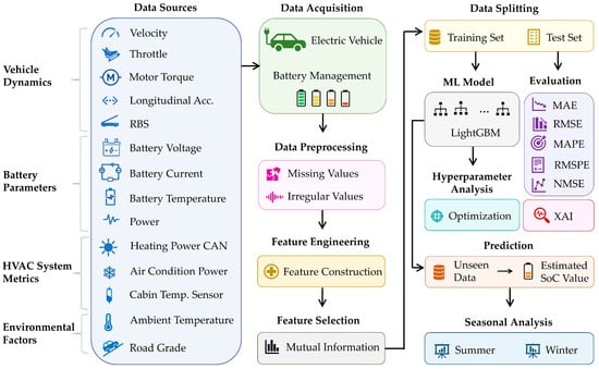
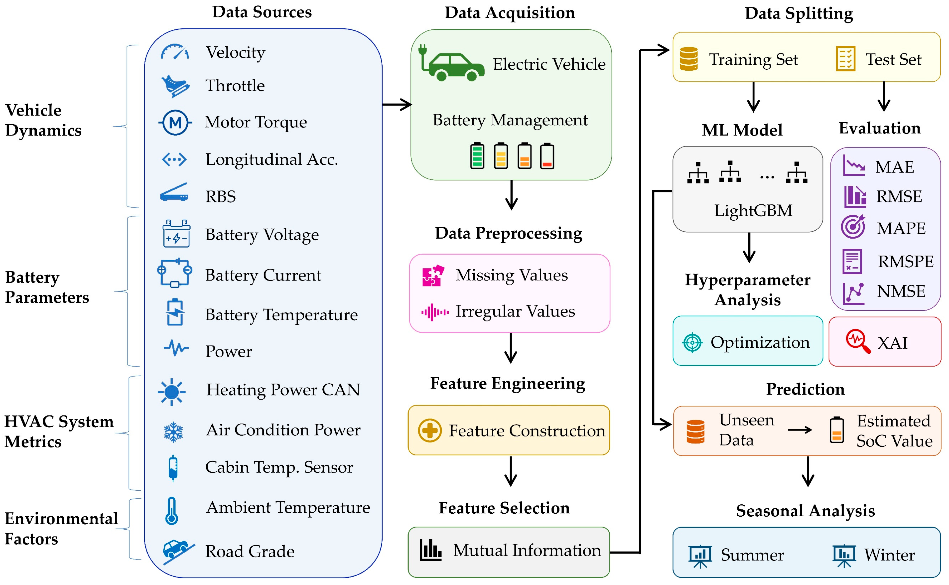
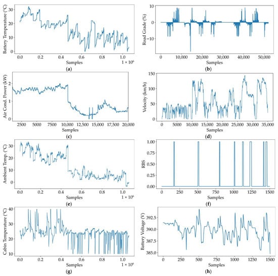
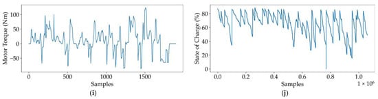
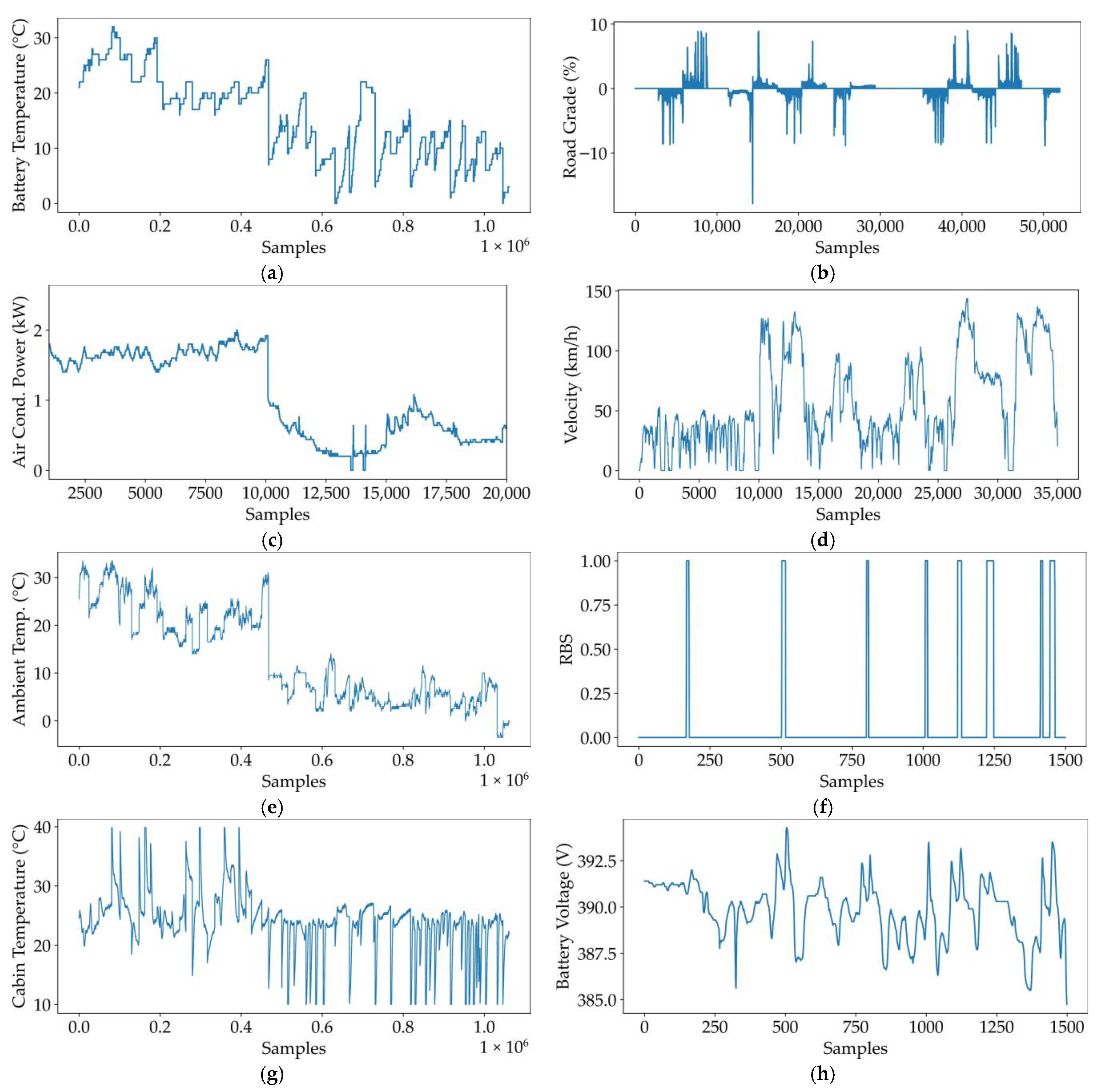
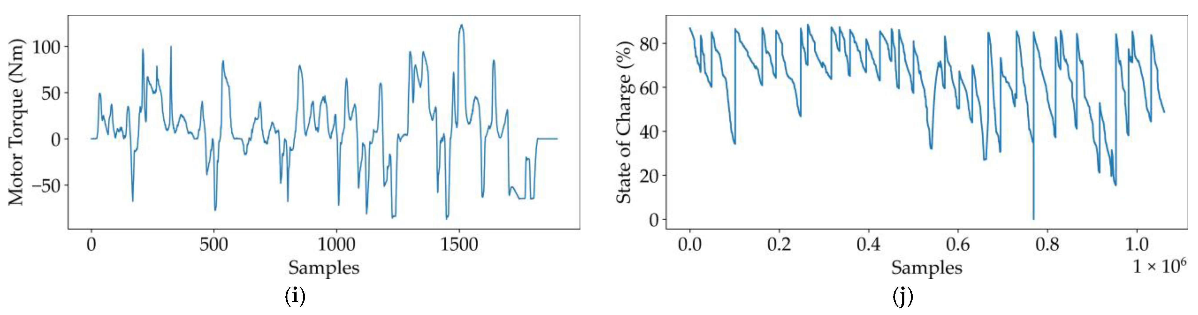
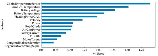
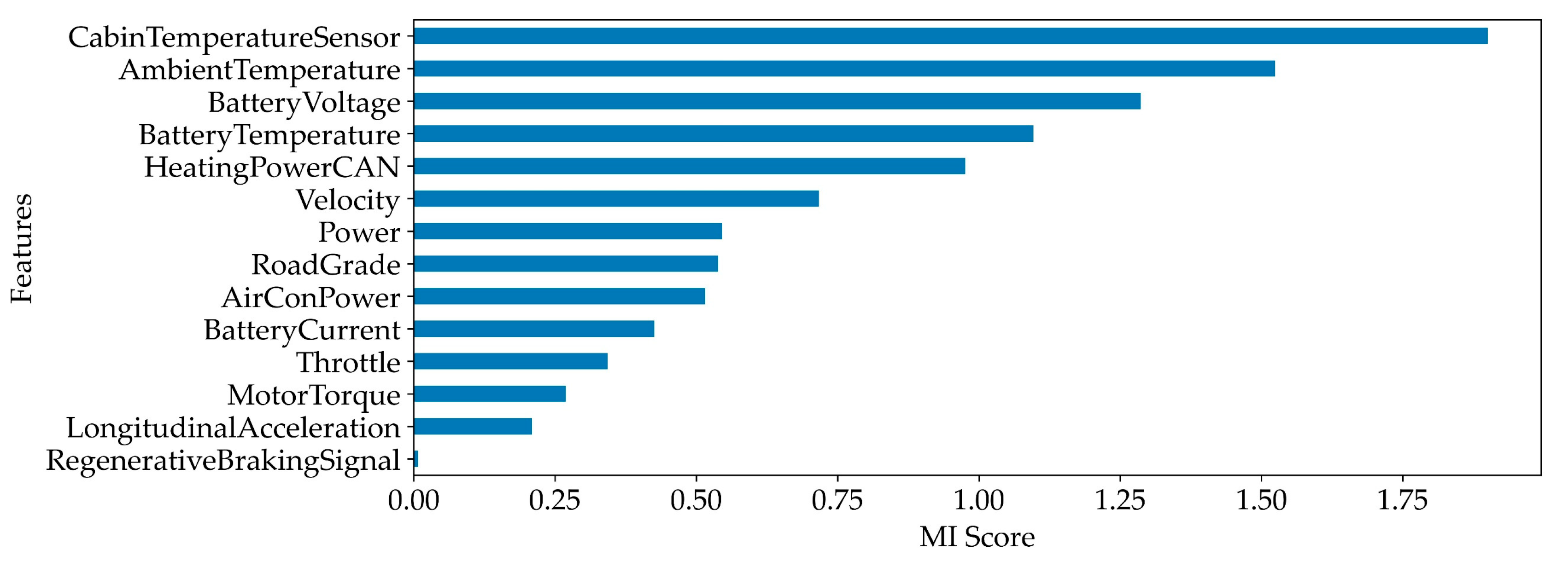
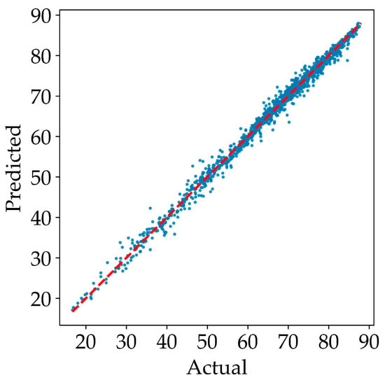
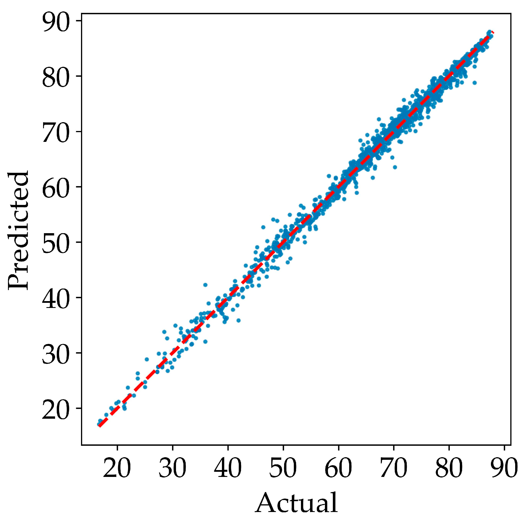
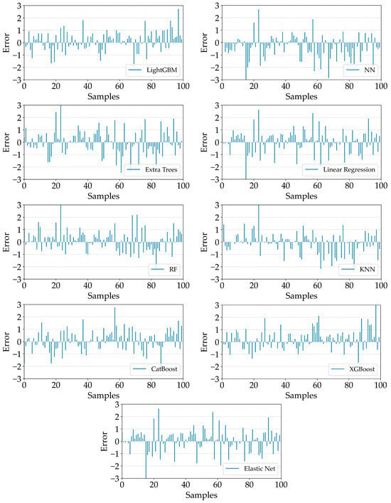
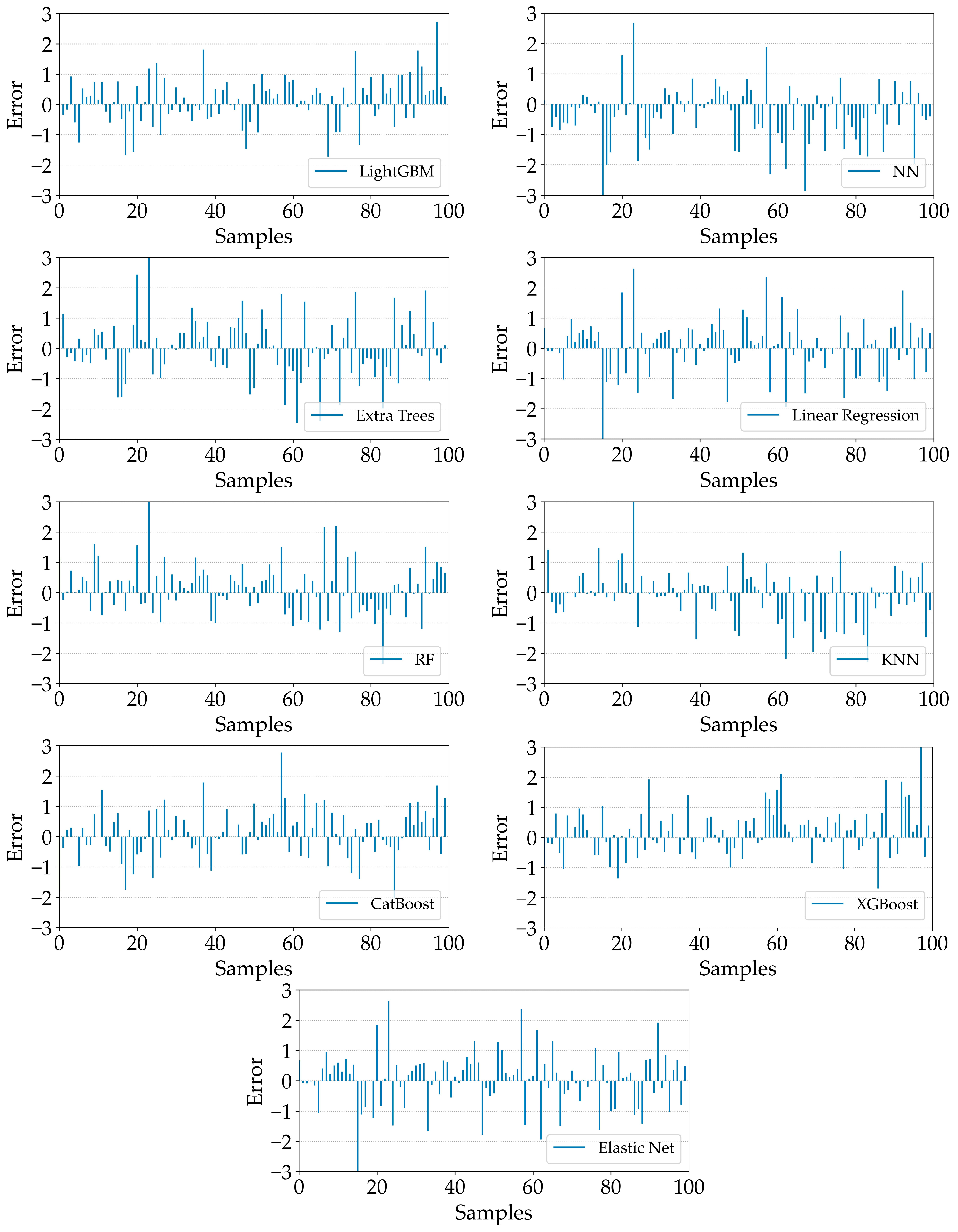
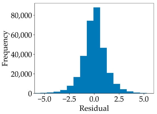
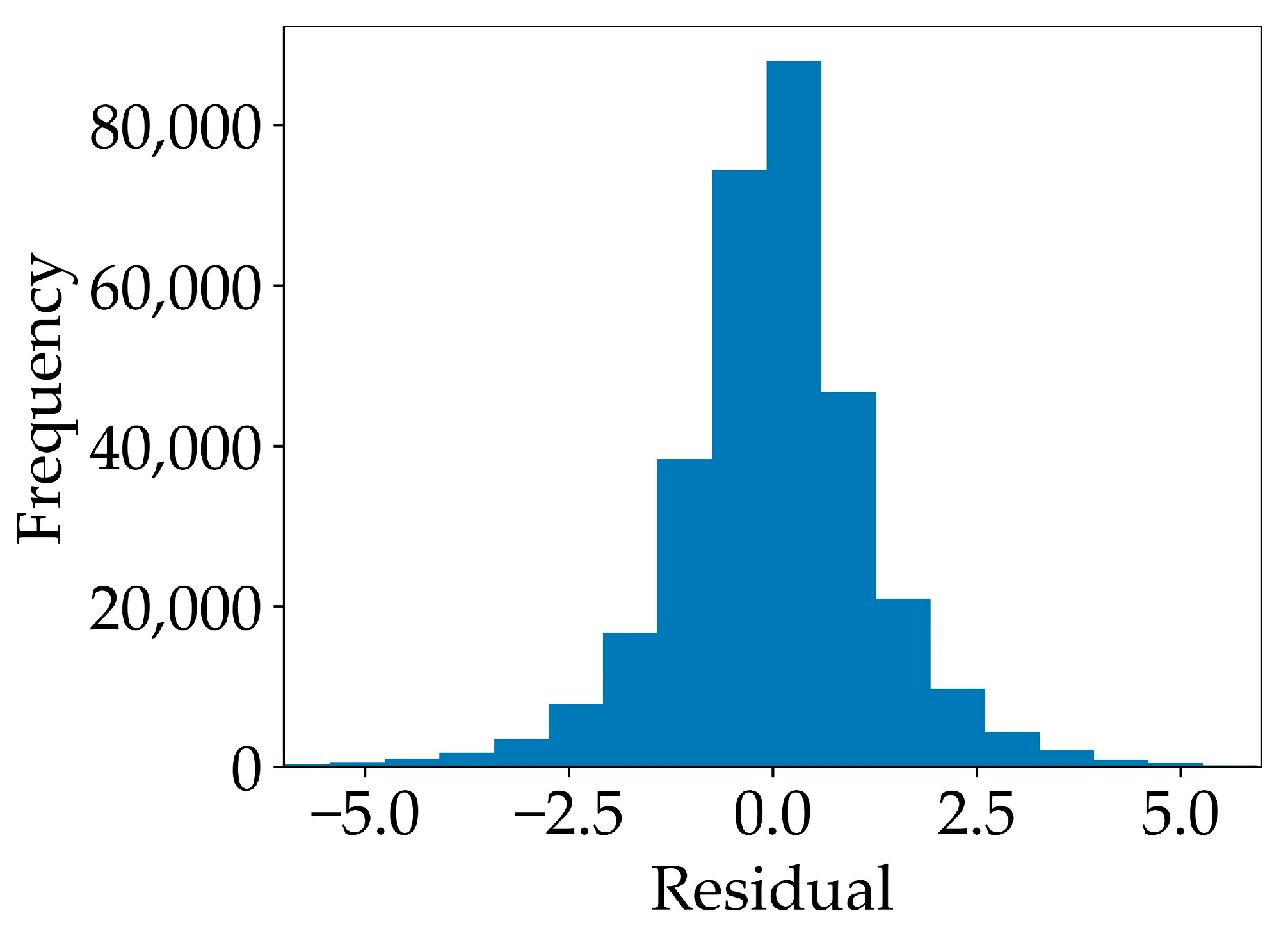
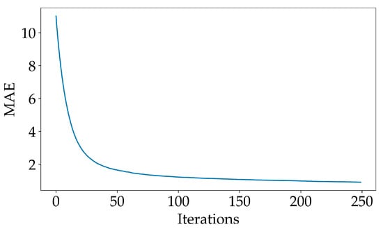
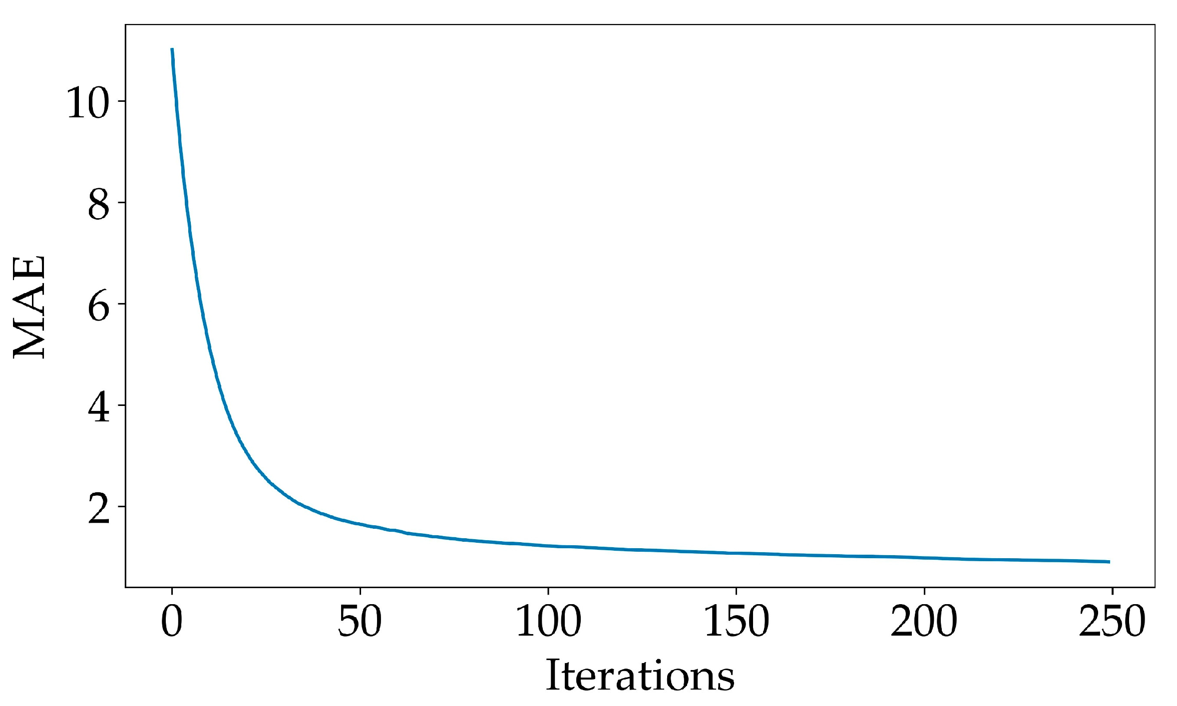
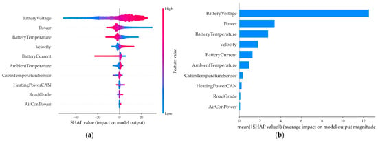
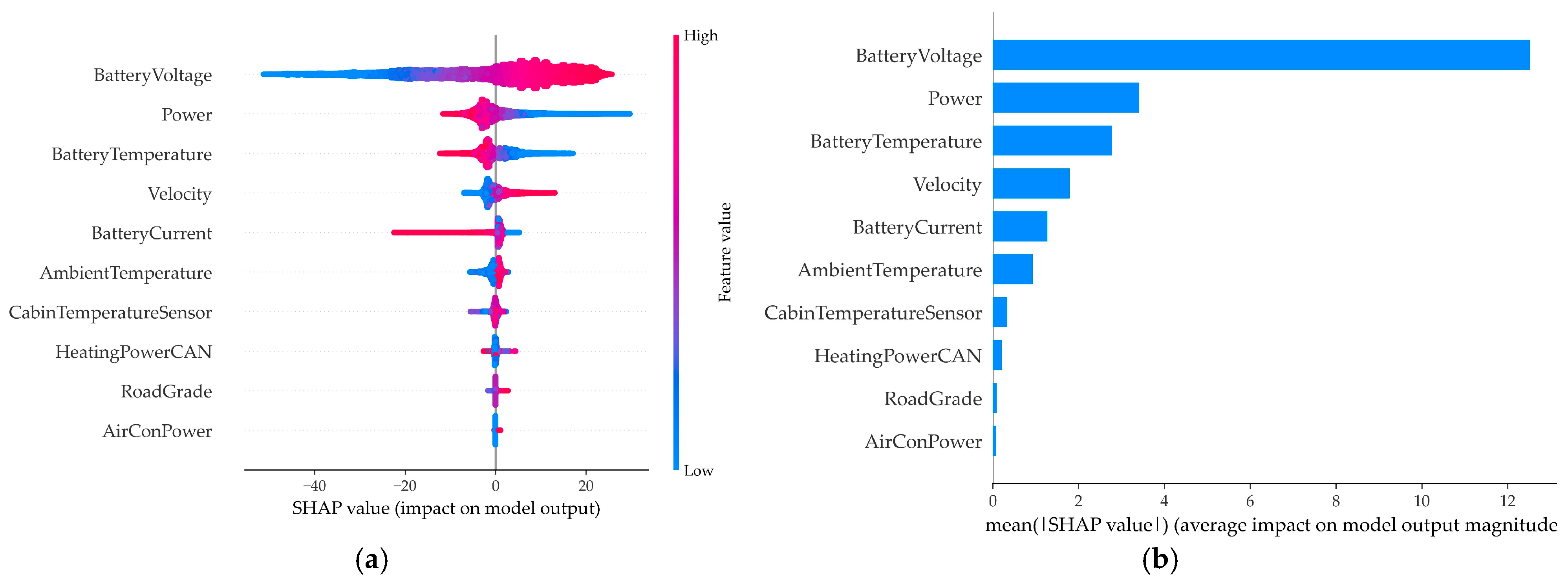
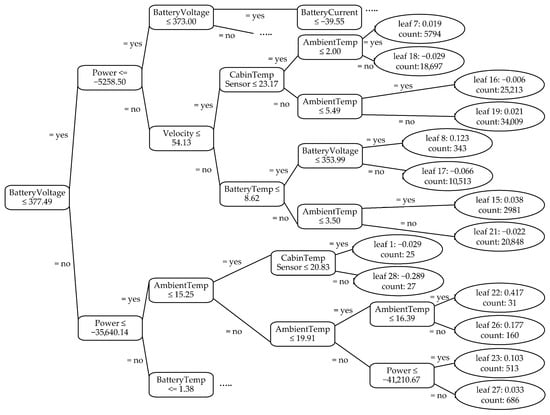
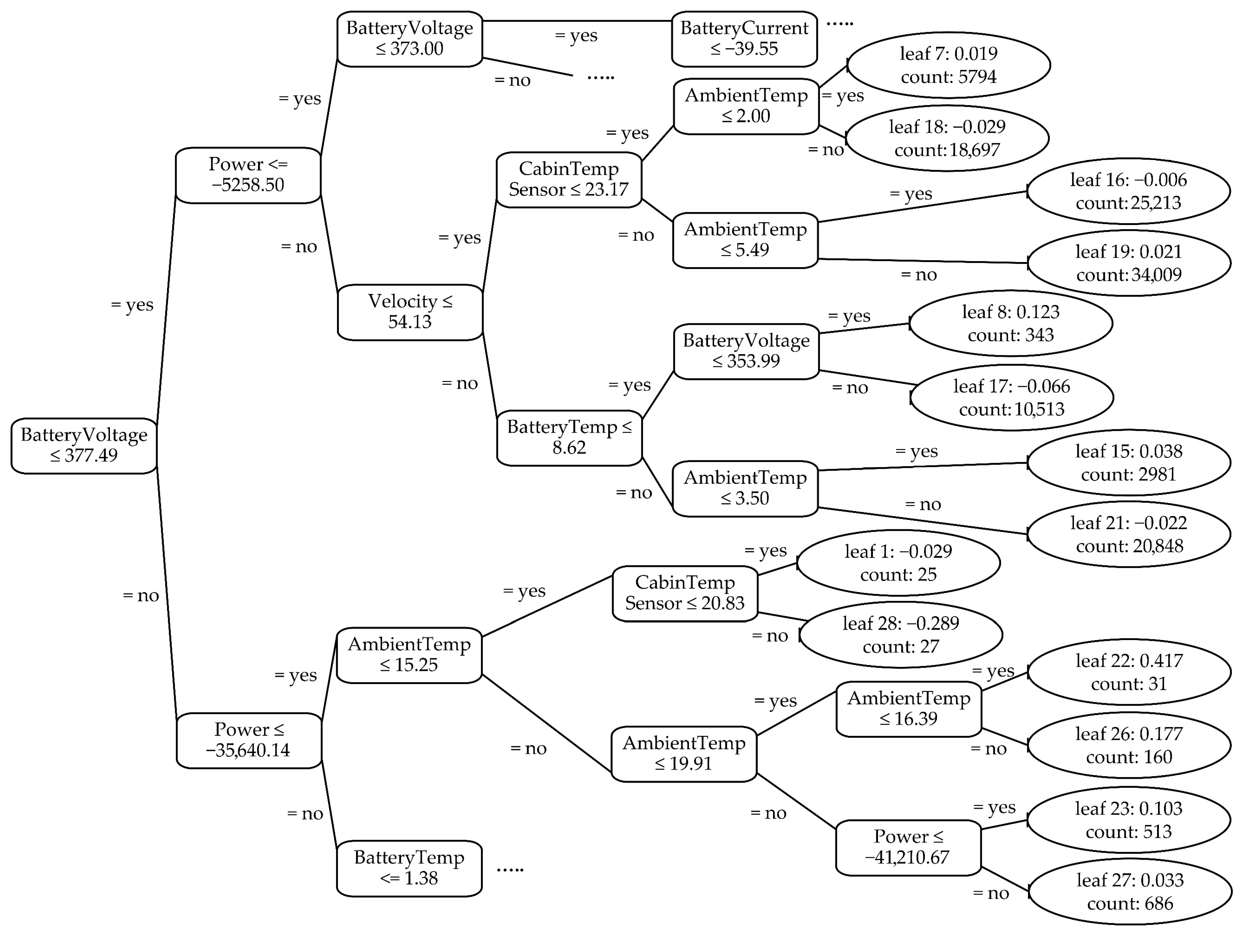
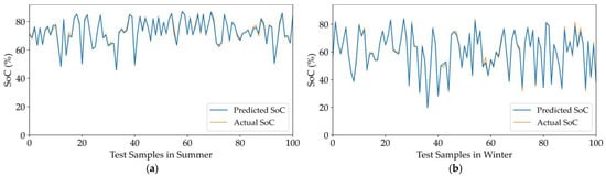
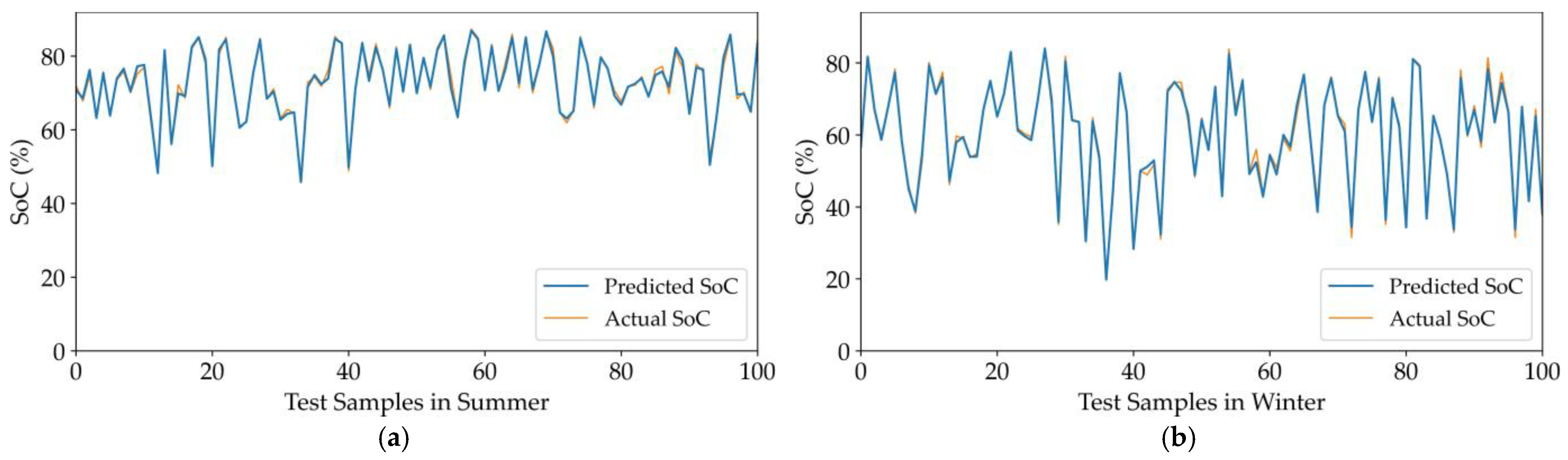

Disclaimer/Publisher’s Note: The statements, opinions and data contained in all publications are solely those of the individual author(s) and contributor(s) and not of MDPI and/or the editor(s). MDPI and/or the editor(s) disclaim responsibility for any injury to people or property resulting from any ideas, methods, instructions or products referred to in the content. |
© 2026 by the authors. Licensee MDPI, Basel, Switzerland. This article is an open access article distributed under the terms and conditions of the Creative Commons Attribution (CC BY) license.