


Abstract
Isothermal dispatch models for battery energy storage systems (BESSs) systematically underestimate degradation costs because dispatch-induced Joule heating elevates cell temperature and accelerates ageing through Arrhenius-type kinetics. This paper proposes three integrated contributions. First, a thermal–electrochemical coupling loop embeds a first-order lumped thermal model within the dispatch simulation: cell temperature is updated from I2R heat generation and Newton cooling at each time step, and the resulting temperature trajectory feeds into the Arrhenius stress factors of a semi-empirical degradation model combining -based calendar ageing with Rainflow-based cycle ageing, enabling the optimiser to discover thermally self-regulating strategies. This coupling is critical because, as the results demonstrate, ignoring it leads to systematic underestimation of degradation costs by up to 13%. Second, the resulting four-objective problem (negative profit, thermally coupled degradation cost, SOC deviation, and CVaR imbalance penalty) is solved by a hypervolume-contribution-enhanced NSGA-III (HVC-NSGA-III), which augments reference-point selection with an archive pruned by removing the solution of the smallest individual hypervolume contribution, concentrating Pareto resolution in the knee region. Third, an SOH-adaptive knee-point selection assigns the degradation weight as a monotone function of ageing degree , automatically tightening dispatch conservatism as remaining useful life diminishes. Simulations on ENTSO-E data over 96 h show the following: (i) thermal coupling shifts the Pareto front by 8–15% in the degradation dimension with temperature excursions up to 7 K; (ii) HVC-NSGA-III improves hypervolume by 8.7% over standard NSGA-III; (iii) SOH-adaptive selection reduces capacity loss by 27.4% at only 9.1% revenue cost; and (iv) ablation confirms Rainflow (24.8%) and thermal coupling (13.1%) as the two largest contributors.
1. Introduction
Large-scale battery energy storage systems (BESSs) have become indispensable components of modern power systems, providing grid services ranging from energy arbitrage and frequency regulation [1] to renewable energy integration and peak shaving [2,3,4]. Recent reviews of battery technologies for next-generation energy storage [5] have further highlighted thermal instability and degradation-aware operation as key barriers to widespread BESS deployment. While this work focuses on lithium-ion BESS, alternative large-scale storage technologies such as redox flow batteries offer distinct advantages in thermal stability, independent energy–power scaling, and potentially longer cycle life [6], which may relax some of the degradation constraints addressed here. The proposed framework is chemistry-agnostic in structure and could be adapted to flow battery systems with appropriate degradation and thermal sub-models.
In the day-ahead electricity market, BESS operators schedule charging during low-price periods and discharging during high-price periods to maximise arbitrage revenue. However, every charge–discharge cycle induces irreversible electrochemical degradation that erodes the battery’s energy capacity and power capability over time, ultimately determining its economic lifetime and replacement cost [7,8].
The central challenge in BESS dispatch is therefore a fundamental conflict between short-term revenue maximisation and long-term asset preservation: aggressive cycling strategies that exploit price volatility yield higher immediate profits but accelerate capacity fade, while conservative strategies preserve battery health at the expense of foregone revenue. Crucially, this trade-off is mediated by thermal dynamics: high-power operation generates Joule heat that elevates cell temperature, which in turn accelerates both calendar and cycle ageing through Arrhenius-type kinetics [7,9]. This thermal–electrochemical coupling creates an additional feedback loop that is ignored by isothermal dispatch models but can significantly alter the optimal operating strategy. Accurately modelling this coupling and embedding the model within an operational optimisation loop is therefore essential for realistic battery management and lifetime prediction in market-facing applications.
1.1. Literature Review
1.1.1. Degradation Modelling in BESS Dispatch
The integration of degradation effects into BESS dispatch has been approached from two directions: constraint-based and cost-based methods [10]. Constraint-based methods limit the depth of discharge (DOD), cycle count, or SOC range to indirectly control degradation, but they do not quantify the degradation cost explicitly and may be overly conservative [11]. Cost-based methods assign a monetary value to each unit of capacity lost and include it in the objective function, enabling a direct economic trade-off between revenue and lifetime [12,13].
Among cost-based approaches, the simplest degradation proxy is the full equivalent cycle (FEC) counter, which assumes a fixed capacity loss per unit of energy throughput [14]. While computationally efficient, the FEC model ignores the well-documented nonlinear dependence of degradation on cycle depth, SOC level, and temperature [7]. More sophisticated models incorporate empirical stress functions derived from accelerated ageing tests, capturing the dependence on DOD, mean SOC, C-rate, and temperature [15,16]. Rainflow cycle-counting algorithms, originally developed for mechanical fatigue analysis, have been adapted to extract cycle features from arbitrary SOC trajectories and provide accurate cycle-by-cycle degradation estimates [17]. However, integrating Rainflow counting into dispatch optimisation remains challenging because of its non-differentiable, path-dependent nature.
A critical limitation shared by nearly all existing degradation-aware dispatch studies is the isothermal assumption: cell temperature is treated as a fixed exogenous parameter rather than as a dynamic state variable coupled to the dispatch decisions [18,19]. In practice, cell temperature varies by several Kelvin over a dispatch horizon due to I2R losses and entropy changes, and this variation has a material impact on ageing rates through the exponential Arrhenius dependence. Moreover, recent studies have shown that the temperature sensitivity of degradation evolves with the battery’s health state: as the cell ages, changes in the SEI morphology and electrode microstructure modify the effective activation energies, leading to an SOH-dependent temperature sensitivity that static Arrhenius models cannot capture [20]. Only a handful of studies in the battery sizing literature have considered thermal dynamics [18], and none have embedded a dynamic thermal model within a many-objective dispatch optimisation loop.
1.1.2. Single- vs. Multi-Objective Dispatch
The vast majority of degradation-aware BESS dispatch studies formulate the problem as a single-objective optimisation, typically minimising total cost (negative revenue plus degradation cost) or maximising net profit after degradation deduction [12,13,21,22]. This approach requires the operator to specify a scalar degradation cost coefficient a priori, which effectively pre-determines the revenue–lifetime trade-off without revealing the full range of available options. In practice, different operators may have vastly different preferences depending on their business model, battery chemistry, warranty conditions, and risk appetite.
Multi-objective optimisation addresses this limitation by computing the entire Pareto front of non-dominated solutions, enabling the operator to visualise the trade-off landscape and select the preferred solution a posteriori. While multi-objective approaches have been applied to microgrid energy management [23] and BESS sizing [18,24], their application to degradation-aware day-ahead BESS dispatch with more than two objectives remains limited. In particular, few studies consider the four-way trade-off among profit, degradation, SOC management, and imbalance risk, simultaneously.
Furthermore, existing multi-objective BESS studies typically model imbalance risk using simple quadratic or absolute-value penalties, which do not distinguish between typical deviations and extreme tail events. Conditional Value-at-Risk (CVaR) [25] provides a coherent alternative that focuses on the worst-case tail of the imbalance distribution. We note that translating day-ahead dispatch schedules into real-time grid operation also requires inverter-level voltage–power coordination, particularly in distribution networks with high penetration of distributed generation [26]; this control layer is outside the scope of the present optimisation framework but represents an important implementation consideration.
1.1.3. Many-Objective Optimisation and Solution Selection
When the number of objectives exceeds three, conventional multi-objective evolutionary algorithms (MOEAs) such as NSGA-II suffer from dominance resistance and loss of selection pressure [27]. The reference-point-based NSGA-III algorithm [28] was specifically designed for many-objective problems and maintains diversity across the Pareto front through structured reference points on a normalised hyperplane. NSGA-III has been successfully applied to power system scheduling [29] but has not been combined with detailed thermal-degradation coupling models for BESS dispatch. Alternative many-objective algorithms (e.g., MOEA/D and DRL-based methods [30]) have also been applied to power system scheduling, but MOEA/D requires careful weight vector specification, and DRL methods typically optimise a scalar reward embedding a fixed preference. The reference-point approach of NSGA-III provides a more natural framework for generating a diverse Pareto front without pre-specifying preference weights.
A known limitation of standard NSGA-III is that its niche-preserving selection does not explicitly maximise the hypervolume indicator, which is the only known unary quality indicator that is strictly Pareto-compliant [31]. Recent work has shown that augmenting reference-point-based algorithms with hypervolume contribution (HVC) information can improve convergence in the knee region of the Pareto front [32]. We propose an HVC-enhanced variant that retains NSGA-III’s diversity mechanism while using hypervolume contributions for archive pruning.
After computing the Pareto front, the operator must select a single solution for implementation. The knee point, defined as the solution offering the greatest simultaneous improvement across all objectives, is a natural choice requiring no explicit preference articulation [33]. However, standard knee-point methods treat all objectives equally, ignoring the fact that conservatism should increase with battery age: aggressive cycling is acceptable when , but each unit of capacity loss removes a growing fraction of remaining useful life as . An SOH-adaptive knee-point strategy that formalises this intuition has not been explored.
1.2. Research Gaps and Contributions
The preceding review reveals that existing studies address individual aspects of degradation-aware dispatch, cycle counting, thermal modelling, multi-objective formulation, or solution selection in isolation, but no unified framework integrates all four elements within a single optimisation loop.
Based on the above analysis, the following gaps are identified: (1) most degradation-aware dispatch studies use single-objective formulations that hide the Pareto trade-off from the operator; (2) FEC-based degradation models oversimplify the nonlinear dependence on cycle depth and SOC level; (3) the isothermal assumption ignores dispatch-induced temperature variations and their feedback on ageing; (4) many-objective algorithms (specifically NSGA-III) have not been applied to BESS dispatch with integrated thermal–Rainflow-based degradation; (5) existing imbalance models lack tail-risk awareness; and (6) post-optimality solution selection lacks degradation-aware and SOH-adaptive mechanisms.
The main contributions of this paper are:
- A thermal–electrochemical co-optimisation formulation that embeds a lumped-parameter thermal model within the dispatch loop, enabling the optimiser to account for dispatch-induced temperature excursions and their feedback on both calendar and cycle ageing. This replaces the static isothermal assumption and provides physically consistent lifetime estimation.
- A four-objective BESS dispatch model that simultaneously considers negative profit, cumulative degradation cost (with thermal coupling), SOC trajectory deviation, and a CVaR-based imbalance risk measure, providing a comprehensive and risk-aware view of the dispatch trade-off landscape.
- A semi-empirical degradation model integrating Rainflow cycle counting with SOC-, C-rate-, and dynamic temperature-dependent stress factors, embedded directly into the multi-objective evaluation loop to provide physically meaningful lifetime cost estimation under realistic thermal conditions.
- An HVC-enhanced NSGA-III (HVC-NSGA-III) variant for the four-objective dispatch problem, combining reference-point-based diversity preservation with hypervolume-contribution-based archive pruning to improve Pareto front quality in the economically critical knee region.
- An SOH-adaptive weighted knee-point selection strategy where the degradation preference weight is automatically modulated as a monotone function of the battery’s current state of health, formalising the principle that remaining lifetime becomes increasingly valuable as the battery ages and enabling lifecycle-aware dispatch without manual parameter tuning.
Collectively, these contributions advance the state of the art in battery modelling and management by demonstrating that even a computationally lightweight thermal model, when embedded within the dispatch optimisation loop, can materially alter strategy selection and that degradation-aware scheduling benefits from physics-informed models that go beyond simple cycle-counting proxies. The simulation-based framework provides a practical tool for evaluating how modelling fidelity translates into operational and economic outcomes.
The remainder of this paper is organised as follows. Section 2 presents the BESS model including SOC dynamics, the thermal model, the semi-empirical degradation model, and the economic model. Section 3 formulates the multi-objective dispatch problem and describes the HVC-NSGA-III solver and SOH-adaptive knee-point selection strategy. Section 4 details the simulation setup. Section 5 presents the numerical results. Section 6 discusses findings, limitations, and practical implications. Section 7 concludes the paper.
2. Battery Energy Storage System Model
For reference, the principal symbols used throughout Section 2 and Section 3 are summarised in Table 1.
Table 1.
Principal nomenclature.
This section presents the mathematical models governing the BESS operation, including SOC dynamics, thermal dynamics, degradation mechanisms, and economic calculations.
2.1. SOC Dynamics and Operational Constraints
Consider a BESS with rated energy capacity (MWh), rated power (MW), and round-trip efficiency . The charge and discharge efficiencies are and , respectively. The SOC at time step is governed by:
where and are the charging and discharging power at time t, respectively, is the time step, and simultaneous charging and discharging is prohibited:
The net power exchanged with the grid is defined as
where indicates discharging (selling) and indicates charging (buying).
The operational constraints are
2.2. Lumped-Parameter Thermal Model
A distinguishing feature of the proposed framework is the inclusion of a dynamic thermal model that tracks cell temperature evolution and feeds it into the degradation calculation. We adopt a first-order lumped-parameter thermal model [7,9]:
where (kg) is the effective cell mass, (J/(kg·K)) is the specific heat capacity, is the heat generation rate, and is the cooling rate.
2.2.1. Heat Generation
The heat generation rate comprises Joule heating and entropic (reversible) heating:
where is the internal resistance (a function of SOC and temperature), is the cell current, and is the entropy coefficient. The cell current is related to the system-level power via
where is the nominal cell voltage and is the number of parallel strings. The SOC- and temperature-dependent internal resistance is modelled as
where is the reference resistance, models the SOC dependence (resistance is lowest near 50% SOC), and is the activation energy for the resistance Arrhenius term. The resistance parameters , , and J/mol are identified from the EIS (electrochemical impedance spectroscopy) measurements reported by Schmalstieg et al. [7] for NMC/graphite 18650 cells at five temperatures (5–45 °C) and three SOC levels (20%, 50%, 80%). The SOC-quadratic form in (12) is a standard parameterisation that captures the U-shaped resistance–SOC characteristic observed experimentally [7,9].
2.2.2. Cooling Model
The cooling is modelled using Newton’s law:
where is the effective heat transfer coefficient (accounting for the thermal management system), is the total surface area, and is the ambient temperature (assumed constant within a scheduling period but potentially varying across days).
The thermal management system (TMS) consumes electrical power proportional to the cooling load [34]:
where is the coefficient of performance of a containerised forced-air unit [34]. This parasitic load is deducted from the net power available for arbitrage.
2.2.3. Discrete-Time Temperature Update
Discretising (9) with a forward Euler scheme yields
This equation is evaluated at each time step alongside the SOC update (1), creating a coupled SOC–temperature trajectory for each candidate dispatch schedule. The key consequence is that the temperature at which degradation is evaluated is endogenous to the dispatch decision: aggressive cycling generates more heat, raises cell temperature, and accelerates ageing beyond what an isothermal model would predict. The thermal update adds negligible computational overhead (less than 5% per evaluation) compared with the Rainflow counting step.
Remark 1
(Scope and limitations of the lumped thermal model). The first-order lumped model (9) captures the dominant time constant of thermal dynamics (typically 30–120 min for containerised BESSs) but does not resolve spatial temperature gradients within the pack. For the purpose of dispatch optimisation at hourly resolution, this level of fidelity is appropriate: the optimiser requires an indication of whether a dispatch strategy causes significant heating relative to alternatives, not a spatially resolved thermal map. Several limitations merit noting. First, the model does not capture cell-to-cell temperature variability (3–5 K in large packs), meaning hot spot cells may degrade faster than the pack average. Second, the fixed-COP cooling assumption does not reflect nonlinear TMS behaviour at extreme conditions. Third, sub-minute thermal transients are smoothed by the hourly discretisation; for high C-rate applications (>1 C), a multi-node thermal model would be more appropriate [5,9]. Despite these limitations, the lumped model captures the dominant thermal feedback relevant to hourly dispatch optimisation. Quantitatively, published comparisons between lumped-parameter and spatially resolved (CFD or multi-node) thermal models for containerised BESS show that the pack-average temperature predicted by the lumped model deviates by less than 1.5 K from the volume-averaged CFD result over hourly time scales [5,18], while intra-pack gradients (captured only by CFD) add 3–5 K at cell-level hot spots. For dispatch optimisation, the relevant quantity is the relative temperature difference between candidate strategies rather than the absolute temperature; the lumped model preserves this ranking faithfully because the gradient bias is approximately strategy-independent. A formal quantification of this ranking preservation against a validated CFD model for the specific pack geometry is left to future experimental work (Section 7). The entropic heating term in (10) is retained for completeness but contributes less than 5% of total heat generation at the C-rates typical of arbitrage operation (≤0.5 C).
Remark 2
(Physical justification of thermal parameters). The effective thermal capacitance = 5.0 × 10⁶ J/K and cooling coefficient = 1.2 × 10³ W/K are consistent with the ranges reported for containerised BESS units [18,34]. The resulting thermal time constant 69 min falls within the 30–120 min range in the experimental literature [7,18].
2.3. Semi-Empirical Degradation Model
Battery degradation, a central challenge in energy storage applications [5,7,8], comprises both calendar ageing (time- and temperature-dependent) and cycle ageing (usage-dependent). We adopt a semi-empirical model that captures both mechanisms, now with dynamic temperature coupling from the thermal model.
2.3.1. Calendar Ageing
Calendar ageing occurs regardless of usage and depends on temperature and SOC level. Unlike prior work that evaluates calendar ageing at a fixed nominal temperature, we evaluate it at the instantaneous cell temperature from the thermal model. The calendar capacity loss over a time interval is
where is the calendar ageing rate function:
with as the pre-exponential factor, as the activation energy (J/mol), as the universal gas constant, T as the absolute cell temperature (K) from the thermal model, and as the SOC acceleration coefficient. The dependence reflects the diffusion-limited nature of solid electrolyte interphase (SEI) growth.
Remark 3
(Temperature sensitivity of calendar ageing). Tang et al. [20] demonstrated that the temperature sensitivity of degradation intensifies with cumulative ageing, as structural changes at the electrode–electrolyte interface modify the effective activation energies; fixed-parameter models can underestimate late-life degradation by 10–20%. This provides independent justification for the SOH-adaptive strategy in Section 3.5: as the battery ages, both the marginal value of remaining capacity and the physical sensitivity to thermal stress increase. The current model uses fixed Arrhenius parameters for tractability; incorporating SOH-dependent activation energies [20] is a natural extension.
According to the Arrhenius law with = 24,500 J/mol, a 10 K increase in cell temperature approximately doubles the calendar ageing rate near the reference temperature of 298 K. Since the thermal model (15) predicts temperature excursions of 3–7 K above ambient during aggressive cycling, the isothermal approximation can in principle underestimate the instantaneous calendar ageing rate by 20–50% relative to ambient conditions during high-power periods. However, because the commonly used isothermal reference temperature (298.15 K) is itself 5 K above the ambient (293.15 K), the net amplification relative to the isothermal baseline is more moderate (5–8% at peak; see Section 5.1). The actual cumulative effect depends on the duration and frequency of the thermal excursions, as calendar ageing accumulates over time via the factor in (16).
2.3.2. Cycle Ageing via Rainflow Cycle Counting
Cycle ageing is evaluated using the Rainflow cycle-counting algorithm, which extracts a set of half-cycles from the SOC trajectory over the scheduling horizon, where is the depth of discharge and is the mean SOC of the j-th extracted cycle.
The capacity loss per half-cycle is modelled using a power-law stress function with temperature coupling:
where the C-rate and temperature stress factors are
and are empirically fitted parameters, is the average C-rate during the j-th cycle, and are reference values, and is the average cell temperature during the j-th cycle, obtained from the thermal trajectory. The Arrhenius temperature factor via activation energy captures the temperature acceleration of cycle ageing independently of calendar effects. The Arrhenius stress factors account for temperature-dependent ageing acceleration, as similarly observed in electrochemical energy systems where temperature sensitivity adapts with cumulative degradation [20]. In the present model, is treated as constant; SOH-dependent activation energies would refine accuracy at advanced degradation states.
The exponent (typically 1.5–2.5 for NMC lithium-ion cells) captures the well-known superlinear relationship between DOD and degradation: a single deep cycle causes more damage than multiple shallow cycles with the same total energy throughput. The exponential SOC term reflects accelerated ageing at high SOC due to increased electrolyte oxidation.
2.3.3. Total Degradation and SOH Update
The total capacity loss over the scheduling horizon is
and the state of health is updated as
where is the initial state of health. The economic end-of-life is typically defined as , so the remaining useful life depends directly on the cumulative degradation incurred by the dispatch strategy.
Remark 4
(Computational treatment of Rainflow counting). The Rainflow algorithm is inherently sequential and non-differentiable, making it incompatible with gradient-based optimisation. In the proposed HVC-NSGA-III framework, this is not a limitation because the evolutionary algorithm evaluates each candidate dispatch schedule by simulating the coupled SOC–temperature trajectory and post-processing it through the Rainflow counter. This simulation-based evaluation naturally accommodates path-dependent, thermally coupled degradation models without requiring differentiability.
Remark 5
(Online parameter estimation for degradation model). The degradation parameters are pre-calibrated from offline ageing data and remain fixed throughout optimisation. In practice, these parameters may drift with ageing [8]. Online methods such as the Padé-approximated P2D model [35] could enable periodic re-calibration within the dispatch loop. Combined with the adaptive weight (46), this would create a doubly adaptive closed-loop system.
2.4. Economic Model
2.4.1. Arbitrage Revenue
The arbitrage revenue over the scheduling horizon is
where (€/MWh) is the day-ahead electricity price at hour t and is the TMS parasitic power consumption defined in (14). The TMS load reduces the effective revenue during both charging (increased grid purchase) and discharging (reduced sellable power) periods. When (discharging), the BESS earns revenue; when (charging), it incurs cost.
2.4.2. Degradation Cost
The degradation cost translates capacity loss into monetary terms using the replacement cost method:
where (€) is the full battery replacement cost and the denominator represents the total usable capacity loss from new () to end-of-life ().
2.4.3. Fixed and Annualised Costs
The hourly fixed cost includes annualised capital expenditure (CAPEX), operation and maintenance (O&M), insurance, and grid connection fees:
where is the capital recovery factor for discount rate r and project lifetime L years, and (€) is the TMS capital expenditure, estimated at 1,200,000 € (6% of total CAPEX) following [34].
Remark 6
(Constant-cost assumption). The costs and are treated as constant present-value parameters. For long-term economic projections, cost escalation indices such as CEPCI [34] should be applied. The constant-cost assumption is justified for the 96 h dispatch horizon; for multi-year lifecycle simulations (Section 5.6), CEPCI-adjusted projections would improve fidelity.
2.4.4. Net Profit
The net profit over the scheduling horizon is
2.5. CVaR-Based Energy Imbalance Model
In practice, the actual BESS output may deviate from the day-ahead schedule due to execution lag, ramp constraints, and real-time re-dispatch. We model the imbalance risk using Conditional Value-at-Risk (CVaR), which provides a coherent risk measure that focuses on the expected cost in the worst-case tail of the imbalance distribution.
The energy imbalance at each time step is defined as
where represents the realised power output, modelled with state-dependent execution jitter:
where is a ramp-dependent jitter amplification factor, reflecting the practical observation that large power ramps incur higher execution uncertainty.
The imbalance cost for scenario s is
where is the imbalance price. The CVaR at confidence level is
where is the number of Monte Carlo scenarios. We use and , so the CVaR represents the expected imbalance cost in the worst 10% of scenarios. This is a key advancement over simple expected imbalance: by penalising tail risk, the CVaR objective steers the optimiser away from dispatch schedules that have acceptable average imbalance but occasionally produce catastrophic deviations (e.g., during steep ramps).
Remark 7
(CVaR vs. expected imbalance). The expected imbalance cost treats all scenarios equally, while focuses on the worst cases. For dispatch schedules with heavy-tailed imbalance distributions (e.g., those with many steep power transitions), the CVaR can be 2–4× the expected value. This asymmetry is consistent with the penalty structure of real European balancing markets, where extreme deviations incur disproportionately high charges.
Remark 8
(Sample size for CVaR estimation). With = 200 scenarios and α = 0.90, the CVaR is estimated from approximately 20 tail scenarios, which provides moderate statistical precision. The resulting CVaR estimate has a coefficient of variation of roughly 22% per evaluation. Because the evolutionary algorithm averages over many evaluations across generations, and we report results over 20 independent runs, the comparative rankings are stable; however, for operational deployment, a larger scenario count (e.g., 1000) or variance-reduction techniques would be advisable to reduce CVaR estimation noise.
2.6. SOC Shape Penalty
To ensure operational readiness and avoid prolonged periods at extreme SOC levels (which accelerate calendar ageing and reduce round-trip efficiency), we introduce an SOC trajectory deviation penalty:
where is a time-varying target SOC profile (e.g., 50% during off-peak hours and 30% before expected price peaks). This penalty discourages the optimiser from parking the battery at 90% SOC for extended periods, which would be optimal for pure arbitrage but detrimental to calendar life.
3. Multi-Objective Optimisation Framework
The overall architecture of the proposed framework is illustrated in Figure 1. The system comprises four interconnected modules: (i) input data preprocessing, (ii) coupled SOC–temperature simulation with semi-empirical degradation and economic evaluation, (iii) four-objective optimisation via HVC-NSGA-III, and (iv) SOH-adaptive knee-point selection with rolling-horizon SOH feedback. The following subsections detail each module.
Figure 1.
Overall framework of the proposed thermal–electrochemical degradation-aware multi-objective BESS dispatch system. The coupled SOC–temperature simulation feeds into the semi-empirical degradation model and economic evaluation; the four objectives are optimised by HVC-NSGA-III; and the SOH-adaptive knee-point selector produces the final dispatch schedule with rolling-horizon SOH feedback.
3.1. Decision Variables and Policy Parametrisation
Rather than optimising the T-dimensional power schedule directly, which would create an excessively large search space for evolutionary algorithms, we adopt a policy parametrisation approach. The dispatch schedule is generated by a parametrised policy with a low-dimensional parameter vector . Specifically, we use a dimensional strategy vector:
where the components parametrise the dispatch rule as
where is the standardised electricity price, is the base power offset, is the price sensitivity, capture diurnal periodicity, is the SOC reference level, is the price threshold separating charge/discharge regimes, are SOC–price interaction coefficients, is a thermal feedback coefficient that reduces power output when the cell is hot (providing implicit thermal management), and is a price–SOC cross-term that modulates aggressiveness based on the joint state. The output is clipped to satisfy the power and SOC constraints (4)–(7).
Remark 9
(Rationale for policy parameterisation). Policy parameterisation reduces dimensionality from T to , making evolutionary search tractable. The thermal feedback term enables the optimiser to discover thermally self-regulating strategies (automatic power throttling when the cell heats up), while captures price–SOC interaction effects inaccessible to additive policies.
Remark 10
(Expressiveness limitations). The 10-parameter policy cannot represent arbitrary dispatch schedules (e.g., higher-order harmonics or abrupt strategy switches beyond ). This trades expressiveness for interpretability and search efficiency; comparison with neural-network policies is left to future work.
3.2. Objective Functions
Given a policy parameter vector , the coupled SOC–temperature trajectory is computed by forward simulation of (1)–(15), and the four objectives are evaluated:
The multi-objective optimisation problem is
subject to the operational constraints (4)–(8) and the thermal dynamics (15), where is the feasible parameter space.
Definition 1
(Pareto dominance). A solution is said to Pareto-dominate (written ) if and only if for all and for at least one j.
Definition 2
(Pareto front). The Pareto front is the set of all non-dominated objective vectors: .
3.3. Constraint Handling
Constraints are handled using a feasibility-first priority scheme combined with a scalar penalty. Define the constraint violation vector:
and the aggregate violation . Note the inclusion of a maximum cell temperature constraint (e.g., 318.15 K = 45 °C) to prevent thermal runaway risk. During selection, feasible solutions () are always preferred over infeasible ones. Among infeasible solutions, the one with smaller V is preferred. Among feasible solutions, Pareto dominance determines selection.
3.4. HVC-Enhanced NSGA-III Algorithm
The four-objective problem (37) is solved using an enhanced variant of NSGA-III [28] that augments reference-point-based selection with hypervolume contribution (HVC) information.
3.4.1. Reference Point Generation
A set of uniformly distributed reference points is generated on the unit simplex in using Das and Dennis’s systematic approach [36]. With p divisions per axis, the number of reference points is , where is the number of objectives. We use , yielding reference points.
3.4.2. Selection Mechanism with HVC Enhancement
The HVC-NSGA-III selection operates in four steps:
- Non-dominated sorting: The combined parent–offspring population is sorted into fronts
- Reference-point association: Each solution in the critical front (the last front to be partially accepted) is associated with its nearest reference point via perpendicular distance in the normalised objective space.
- Niche-preserving selection: Solutions associated with under-populated niches (reference points with fewer associated members) are preferentially selected, maintaining diversity.
- HVC-based archive pruning (new): An external archive of bounded size is maintained. When exceeds the limit, the solution with the smallest individual hypervolume contribution is removed:where denotes the hypervolume indicator computed with respect to a reference point set at the nadir point. This step preferentially retains solutions in the knee region, where each solution contributes maximally to the hypervolume.
Remark 11
(Complementarity of reference points and HVC). Reference-point-based selection ensures uniform coverage across the Pareto front, while HVC-based archive pruning ensures that the retained solutions are those contributing most to the hypervolume indicator, which is concentrated in the knee region. The two mechanisms are complementary: the former prevents the population from collapsing to the knee, while the latter ensures that the economically important knee region is well resolved.
3.4.3. Genetic Operators
Simulated Binary Crossover (SBX)
For parent values and , the offspring are
where is a spread factor sampled from a polynomial distribution controlled by the crossover distribution index :
Polynomial Mutation
A perturbation is applied with probability :
where is drawn from a polynomial distribution controlled by the mutation distribution index .
3.4.4. Convergence Criterion
The procedure is summarised in Algorithm 1. The algorithm terminates after generations or when the hypervolume indicator [31] of the non-dominated set changes by less than over 20 consecutive generations.
| Algorithm 1 HVC-NSGA-III for Thermal-Degradation-Aware BESS Dispatch |
|
3.5. SOH-Adaptive Knee-Point Selection
After obtaining the Pareto front , the operator must select a single solution for implementation. We propose an SOH-adaptive weighted knee-point strategy that automatically adjusts the degradation preference based on the battery’s current health state.
3.5.1. Normalisation
The objective vectors are normalised to using the ideal and nadir points:
where and .
3.5.2. Weighted Knee-Point Score
The knee-point score for the k-th solution is defined as
where with are objective weights. The knee point is the solution maximising the minimum weighted normalised improvement:
3.5.3. SOH-Adaptive Degradation Weighting
The key innovation is to make the degradation weight a monotone decreasing function of SOH. The intuition is straightforward: when the battery is new (), each unit of capacity loss represents % of the total usable life; when , each unit represents % of the remaining usable life (since only 5% remains before EOL at ). Thus, the marginal value of preserving capacity increases as the battery ages.
We propose the following adaptive weight:
where is the minimum degradation weight (applied when , i.e., brand-new battery) and is the maximum weight (applied when , i.e., end-of-life). The remaining objective weights are
For the default parameters , , and :
- New battery (): —moderately balanced;
- Mid-life (): —degradation-aware;
- Near-EOL (): —strongly conservative.
Proposition 1
(Monotonicity of lifetime preference). The SOH-adaptive weight (46) satisfies the following: (i) is monotonically decreasing in ; i.e., older batteries receive a higher degradation weight; (ii) the selected knee point moves monotonically towards the minimum-degradation extreme as decreases; and (iii) for any fixed Pareto front, the capacity loss of the selected solution is non-increasing in the degradation weight.
Remark 12
(Rolling-horizon SOH coupling). In a rolling-horizon implementation, the SOH at the start of each scheduling period is updated using the degradation incurred in the previous period. The adaptive weight (46) then automatically adjusts the dispatch conservatism for the next period, creating a closed-loop lifecycle management system: early in the battery’s life, the operator captures more arbitrage revenue; as the battery ages, the system becomes progressively more conservative, extending the asset’s remaining useful life. This lifecycle adaptation occurs without any manual parameter tuning.
Remark 13
(Advantage over scalarisation). Unlike single-objective scalarisation , which can miss solutions on non-convex regions of the Pareto front, the proposed knee-point selection operates a posteriori on the already-computed Pareto front. It can identify balanced solutions on non-convex regions and the operator can interactively adjust (or override the SOH-adaptive default) and immediately observe the resulting solution on the Pareto front without re-running the optimisation.
4. Simulation Setup
4.1. BESS Parameters
The BESS parameters are listed in Table 2, representative of a utility-scale lithium-ion NMC system.
Table 2.
BESS parameters.
4.2. Thermal Model Parameters
The lumped-parameter thermal model parameters are listed in Table 3, representative of a containerised BESS with forced-air cooling.
Table 3.
Thermal model parameters.
4.3. Degradation Model Parameters
The semi-empirical degradation parameters are calibrated to NMC/graphite lithium-ion cells based on published ageing data [15,16], as listed in Table 4.
Table 4.
Degradation model parameters.
Parameter Justification and Chemistry Assumptions
The calendar parameters are fitted by Ecker et al. [15] to storage tests at 5 temperatures and 3 SOC levels over 9 months. The cycle parameters are fitted by Naumann et al. [16] to cycling data at multiple DOD levels and C-rates. The C-rate exponent and cycle activation energy are from Schmalstieg et al. [7]. These parameters have been widely reused in the dispatch literature [12,13,37] for NMC chemistry.
Mechanisms not explicitly captured include lithium plating, transition metal dissolution, and mechanical particle cracking. The additive superposition in (20) may overestimate degradation by 5–15% when calendar and cycle ageing share SEI pathways [7,8], or underestimate it by up to 20% when deep cycling creates fresh surface area [8]. For the operating regime of this study (, K, C), the error is expected at 5–10%, bounded and insufficient to alter the relative ranking of strategies. The framework is chemistry-agnostic in structure but requires parameter re-identification for other chemistries (e.g., LFP) [16].
4.4. Model Calibration and Limitations
The degradation parameters are adopted from cell-level ageing tests [15,16]; pack-level effects (cell-to-cell variability, balancing losses) introduce additional uncertainty. The lumped thermal model cannot resolve intra-pack hot spots; absolute temperature predictions are indicative, but the relative thermal discrimination among candidate strategies is reliable for dispatch optimisation at hourly resolution. The literature cross-validation shows that predicted calendar loss rates (≈1.8%/year at 25 °C, 50% SOC) are within 15% of Ecker et al. [15], cycle degradation per FEC (≈0.025%) is consistent with Schmalstieg et al. [7], and temperature excursions (3–7 K) align with [5,18]. These comparisons provide evidence that the model operates within a physically plausible regime.
The superposition error (5–10% for the present operating conditions) is small relative to the 13–25% inter-method differences reported in the ablation study (Section 5.8). A dedicated sensitivity analysis of the key degradation and thermal parameters is provided in Section 5.10, which quantifies the model’s robustness to ±variations in , , , , and . The relative ranking of methods is preserved across all parameter perturbations tested.
4.5. Electricity Market Data
All price time series are derived from the ENTSO-E Transparency Platform with a temporal resolution of 1 h. The data set covers a 96 h (4-day) period from the German–Luxembourg (DE-LU) bidding zone, spanning Monday 6 March to Thursday 9 March 2023, selected for its representative diurnal price pattern with morning and evening peaks. Data were downloaded via the ENTSO-E Restful API in hourly resolution; preprocessing consisted of (i) forward-filling of three missing hourly entries caused by daylight-saving-time transitions, (ii) removal of negative price spikes below €/MWh (none occurred in this window), and (iii) conversion from €/MWh to the simulation unit system. The resulting average day-ahead price is approximately 65 €/MWh with an intraday spread of 30–45 €/MWh, providing sufficient arbitrage opportunity. To assess market-dependence, we repeated the full optimisation on a second 96 h window from the French (FR) bidding zone (13–16 June 2023, mean price 58 €/MWh, spread 25–38 €/MWh); the relative ranking of all methods was preserved, with absolute profit levels scaling proportionally to the price spread. The imbalance price is set at 1.5 times the day-ahead price, i.e., . The ramp-dependent jitter parameters are MW and , and the CVaR confidence level is with Monte Carlo scenarios.
4.6. HVC-NSGA-III Configuration
The hyperparameters of the HVC-NSGA-III algorithm are listed in Table 5.
Table 5.
HVC-NSGA-III hyperparameters.
4.7. Baseline Methods
The following baselines are compared:
- MaxProfit: Single-objective profit maximisation ignoring degradation (linear programme, isothermal).
- FEC-Penalised: Single-objective profit maximisation with FEC-based degradation cost penalty (isothermal), i.e., .
- NSGA-II-4obj: Standard NSGA-II applied to the four-objective problem with thermal coupling (to assess the benefit of NSGA-III’s reference-point mechanism).
- NSGA-III-Isothermal: NSGA-III with Rainflow degradation but without the thermal model (fixed K), to isolate the thermal coupling effect.
- NSGA-III-Unweighted: The proposed HVC-NSGA-III framework with thermal coupling but standard (equal-weight) knee-point selection ().
- HVC-NSGA-III-SOHAdapt (Proposed): The full proposed framework with thermal coupling, HVC archive, and SOH-adaptive knee-point selection.
- MOEA/D-4obj: The MOEA/D algorithm [38] with Tchebycheff decomposition applied to the same four-objective thermally coupled problem, using 165 uniformly distributed weight vectors (matching the NSGA-III reference-point count) and neighbourhood size . This baseline tests whether decomposition-based search can match reference-point-based selection for this problem.
The baselines are chosen to isolate the contribution of each proposed module (thermal model, Rainflow degradation, NSGA-III reference points, HVC archive, SOH-adaptive weighting) through progressive ablation. We acknowledge that the single-objective baselines (MaxProfit, FEC-Penalised) represent relatively simple strategies; they are included as widely adopted industry benchmarks rather than as state-of-the-art competitors. An MPC baseline is included to represent optimisation-based receding-horizon control.
An MOEA/D baseline is now included (Section 5.5). A comparison with DRL-based dispatch remains deferred to future work: embedding the non-differentiable Rainflow counter and Monte Carlo CVaR within a DRL reward function requires substantial architectural design (e.g., differentiable surrogate degradation models) to ensure a fair comparison under identical thermal-degradation coupling conditions.
Remark 14
(Impact of TMS power consumption on reported results). The TMS parasitic load reduces net revenue by 12–18 € over 96 h (<0.16% of gross revenue), and the TMS capital cost adds 8.7 € per period uniformly to all methods; neither affects comparative rankings (Section 5.5).
4.8. Statistical Validation Protocol
To account for the stochastic nature of evolutionary algorithms and the Monte Carlo CVaR evaluation, each method is run 20 times with independent random seeds. Performance metrics are reported as mean ± standard deviation, and statistical significance is assessed using the Wilcoxon rank-sum test with a significance level of .
5. Results
5.1. Thermal Profile Analysis
Figure 2 reveals that aggressive dispatch strategies induce predicted cell temperature excursions of up to 7 K above the ambient temperature (from 293.15 K to approximately 300 K) during peak discharging periods. According to the model, this temperature elevation increases the instantaneous calendar ageing rate by 5–8% during peak discharge periods relative to the isothermal assumption at 298.15 K. Conservative strategies keep the predicted temperature within 2 K of ambient. The thermal model also predicts an asymmetric heating pattern: discharging generates more heat than charging at the same power level due to the SOC dependence of internal resistance (12) (resistance is higher at low SOC, which coincides with deep discharge). This asymmetry is invisible to isothermal models and, within the model, shifts the Pareto front measurably towards higher degradation at the aggressive end. While the absolute temperature values depend on the lumped-model parameters (Section 4.4), the qualitative pattern of asymmetric, dispatch-induced heating is physically well founded [7,9].
Figure 2.
Cell temperature trajectories (a) and corresponding calendar ageing rate amplification (b) for three representative Pareto-optimal dispatch strategies. The isothermal assumption (dashed line at 298.15 K) is shown for reference.
5.2. Pareto Front Analysis
Figure 3 displays a three-dimensional projection of the Pareto front. Several observations emerge. First, the front exhibits a distinctly non-convex structure, confirming that weighted-sum scalarisation would miss solutions in the concave region—a key advantage of the population-based HVC-NSGA-III approach. Second, moving along the front from the profit-maximising extreme towards the minimum-degradation extreme, the degradation cost decreases steeply at first and then flattens, indicating diminishing marginal returns of degradation reduction at the cost of revenue. Third, the SOC deviation objective (z-axis) is anti-correlated with both profit and degradation, reflecting the trade-off between operational flexibility and asset preservation. The colour scale reveals that the CVaR imbalance risk is highest for aggressive strategies (high profit, high degradation, many steep ramps) and lowest for conservative strategies.
Figure 3.
Three-dimensional projection of the four-objective Pareto front obtained by HVC-NSGA-III with thermal coupling, projected onto the (Profit, Degradation Cost, SOC Deviation) subspace. The colour scale indicates the fourth objective (CVaR Imbalance Risk). The marked points denote the profit-maximising extreme, the minimum-degradation extreme, the standard knee point, and the proposed SOH-adaptive knee point. The grey surface shows the Pareto front obtained without thermal coupling for comparison.
Critically, the comparison with the isothermal Pareto front (grey surface) reveals that thermal coupling shifts the degradation-heavy portion of the front upward by 8–15%, confirming that isothermal models systematically underestimate the true degradation cost of aggressive strategies. The two fronts converge in the conservative region, where thermal excursions are minimal.
5.3. Dispatch Schedule Comparison
Figure 4 compares the dispatch schedules of three Pareto-optimal solutions over the 96 h horizon. The profit-maximising extreme (a) performs deep daily cycles (SOC swinging between 12% and 90%), exploiting the full price spread but accumulating rapid degradation and reaching peak cell temperatures of 300 K. On days with strong price spreads (Days 2 and 4), the strategy charges the battery to its upper SOC limit during low-price hours and then discharges aggressively during peaks; on the low-spread Day 3, activity is notably reduced. The minimum-degradation extreme (c) adopts an ultra-conservative strategy with shallow cycles (SOC between 38% and 62%), barely responding to price signals and keeping the cell within 1.5 K of ambient. The proposed SOH-adaptive knee point (b) finds a middle ground: it performs moderate-depth cycles (SOC between 24% and 76%) that capture most of the price spread while significantly reducing the DOD per cycle. Notably, the learned thermal feedback coefficient () in the proposed solution is negative, meaning the policy automatically throttles power output when the cell heats up, providing an emergent thermal management behaviour.
Figure 4.
The 96 h dispatch schedules for three representative Pareto-optimal solutions: (a) profit-maximising extreme (red), (b) proposed SOH-adaptive knee point (blue), and (c) minimum-degradation extreme (green). (Top) Electricity price (yellow shaded area) and net power (bars, positive = discharging, negative = charging); (Middle) SOC trajectory (solid line) and cell temperature (dashed line); (Bottom) cumulative capacity degradation.
5.4. SOC Trajectory and Degradation Profile
Figure 5 shows the SOC trajectories, temperature profiles, and cumulative degradation for six representative methods. The MaxProfit strategy produces the deepest cycles, highest temperatures, and highest cumulative degradation (). The FEC-Penalised strategy reduces degradation moderately but still permits deep cycles because the linear FEC model underestimates the cost of high-DOD events. The NSGA-III-Isothermal method achieves lower degradation than FEC but underestimates the true degradation by 11.3% compared to the thermally coupled evaluation, confirming the isothermal bias. The proposed HVC-NSGA-III-SOHAdapt strategy achieves the lowest degradation among strategies with non-trivial revenue.
Figure 5.
SOC trajectories (a), cell temperature trajectories (b), and cumulative degradation profiles (c) for six representative methods over the 96 h scheduling horizon.
The MPC-Isothermal baseline achieves higher gross profit (11,934 €) but 26.6% higher degradation cost and 25.5% higher capacity loss than the proposed method, due to the linear FEC model and absence of thermal coupling. Its CVaR cost is also higher (312 vs. 198 €). The proposed method achieves higher profit-after-degradation (10,200 vs. 10,063 €) despite lower gross revenue, confirming that accurate degradation modelling and thermal coupling yield superior net economic outcomes.
5.5. Quantitative Performance Comparison
Table 6 presents the quantitative results. The proposed HVC-NSGA-III-SOHAdapt method achieves the best overall trade-off: while its gross profit (11,678 €) is 9.1% lower than MaxProfit, its degradation cost is 43.2% lower (1478 vs. 2604 €), yielding the highest profit after degradation (10,200 €). The capacity loss is reduced by 42.8% ( vs. ). To provide intuition for lifetime implications, a simple linear extrapolation (holding degradation rates constant) suggests that MaxProfit would reach EOL () approximately 3 years earlier than the proposed strategy over a 15-year project. However, this extrapolation should be treated with caution: actual degradation rates are nonstationary, market conditions evolve, and the degradation model itself has calibration uncertainty (see Section 4.4). The comparative ranking is nonetheless robust because it derives from the same model applied consistently to all methods.
Table 6.
Quantitative performance comparison over the 96 h scheduling horizon. For the proposed method, mean ± std over 20 independent runs is reported. For other evolutionary methods (NSGA-II, MOEA/D, NSGA-III variants), the mean over 20 runs is reported; standard deviations are of comparable magnitude to the proposed method (omitted for compactness). MaxProfit and FEC-Penalised are deterministic and produce a single result. † Indicates statistically significant difference from the proposed method (Wilcoxon rank-sum, ). NSGA-III-Unweighted differences are not statistically significant at due to overlapping run distributions with the proposed method.
The comparison between NSGA-III-Isothermal and the proposed method reveals that thermal coupling contributes an additional 11.6% reduction in capacity loss (from 3.37 to ), confirming that the dynamic thermal model enables the optimiser to discover thermally aware strategies that are invisible to isothermal formulations.
The HVC enhancement contributes 8.7% higher hypervolume compared to standard NSGA-III (4.23 vs. ), confirming that the archive pruning mechanism improves Pareto-front quality.
The FEC-Penalised baseline achieves moderate degradation reduction but still permits high-DOD cycles ( vs. 0.47), confirming that the linear FEC model underestimates deep-cycle damage. The comparison between NSGA-II-4obj and HVC-NSGA-III demonstrates the superiority of reference-point-based selection with HVC: the proposed method achieves 31.8% higher hypervolume and all differences are statistically significant ().
The MOEA/D baseline achieves a hypervolume of , which is 15.4% lower than the proposed method and 8.0% lower than standard NSGA-III. This confirms that the Tchebycheff decomposition, while effective for two- and three-objective problems, suffers from weight vector sensitivity in the four-objective setting: certain weight directions fail to find feasible solutions when thermally coupled constraints are active, leaving coverage gaps on the Pareto front. The reference-point mechanism of NSGA-III, combined with HVC archive pruning, provides more robust coverage for this problem structure.
5.6. SOH-Adaptive Knee-Point Sensitivity Analysis
Figure 6 shows how the SOH-adaptive mechanism progressively shifts the selected solution along the Pareto front as the battery ages. At , selects a relatively aggressive knee point with higher profit and moderate degradation. At , shifts to a more conservative solution. At , selects a strongly conservative solution that prioritises lifetime preservation. The transition is smooth and monotone, confirming the desired lifecycle behaviour.
Figure 6.
Effect of SOH-adaptive weight on the selected knee-point solution at different battery ages. (a) Degradation weight trajectory; (b) net profit and degradation cost at selected knee points; (c) capacity loss and SOC deviation.
Compared with a fixed-weight strategy (), the SOH-adaptive approach achieves approximately 4.2% higher cumulative revenue over a simulated 5-year lifecycle (constructed by rolling the 96 h optimisation forward with inter-period SOH updates) while maintaining equivalent total degradation. This improvement arises because the adaptive weight captures more arbitrage revenue during the early years when the battery can afford aggressive cycling. We note that this lifecycle simulation assumes stationary market price statistics and does not account for potential long-term trends in electricity prices or evolving grid conditions, which could affect the magnitude (though likely not the direction) of this advantage.
5.7. Rainflow Cycle Distribution
Figure 7 visualises the extracted Rainflow cycles in three dimensions (DOD, mean SOC, and mean temperature). The MaxProfit strategy produces a bimodal DOD distribution with a significant cluster at DOD and elevated cycle temperatures ( K), which incurs disproportionate degradation due to the superlinear stress function () amplified by the Arrhenius temperature factor. The proposed strategy shifts the DOD distribution towards shallower cycles ( vs. 0.48), reduces the mean SOC of the extracted cycles ( vs. 0.52), and lowers the mean cycle temperature ( K vs. 296.7 K). This three-way improvement demonstrates that the optimiser has learned to exploit the nonlinear thermal-degradation coupling by performing cooler, shallower cycles at lower mean SOC levels.
Figure 7.
Rainflow cycle distribution (DOD histogram, mean-SOC scatter, and mean-temperature scatter) for MaxProfit, FEC-Penalised, NSGA-III-Isothermal, and the proposed HVC-NSGA-III-SOHAdapt strategy.
5.8. Mechanism Ablation
Table 7 shows that each module contributes measurably to the overall performance, though the magnitudes vary considerably—from a modest 2.0% (CVaR on degradation) to a substantial 24.8% (Rainflow model). The two largest contributors are the Rainflow degradation model and the SOC shaping objective, underscoring the importance of accurate degradation modelling in dispatch optimisation.
Table 7.
Mechanism ablation: impact of removing individual components from the full framework (HVC-NSGA-III-SOHAdapt). The “” columns show percentage change relative to the full method. All values are mean over 20 runs.
- Thermal model (+13.1% capacity loss): Removing the thermal model reverts to isothermal evaluation, causing the optimiser to underestimate degradation from aggressive strategies and select solutions with 13.1% higher true capacity loss. This is the most significant finding: thermal coupling is not merely a modelling refinement but materially changes the optimal dispatch strategy.
- Rainflow model (+24.8%): Replacing the Rainflow degradation model with the simpler FEC model increases capacity loss by 24.8%, confirming that the nonlinear cycle-depth dependence is essential for accurate degradation-aware dispatch.
- SOC shaping (+20.1%): Removing the SOC shaping objective () increases SOC deviation by 114% and capacity loss by 20.1%, demonstrating that controlling the SOC trajectory indirectly reduces calendar ageing and extreme-SOC operation.
- CVaR vs. expected (+2.0%, but +75% imbalance): Replacing CVaR with the expected imbalance has minimal impact on degradation but increases the CVaR imbalance cost by 75%, confirming that the CVaR objective is essential for tail-risk control.
- SOH-adaptive weighting (+15.8%): Reducing the degradation weight to equal weighting increases capacity loss by 15.8%, confirming the value of the SOH-adaptive knee-point selection.
- HVC archive (+4.7%): Removing the HVC archive pruning increases capacity loss by 4.7% and reduces the hypervolume, confirming that the HVC mechanism improves the quality of solutions in the knee region.
- NSGA-III vs. NSGA-II (+21.5%): Replacing NSGA-III with NSGA-II degrades both profit () and capacity loss (), confirming the superiority of reference-point-based selection for four-objective problems.
5.9. Convergence Behaviour
Figure 8 shows the convergence of the hypervolume indicator. HVC-NSGA-III converges to a higher final hypervolume () than standard NSGA-III () and NSGA-II (). The HVC-enhanced variant reaches 95% of the final hypervolume at generation ∼160 vs. ∼190 for standard NSGA-III and ∼280 for NSGA-II. The faster convergence is attributed to the combined effect of structured reference points maintaining uniform coverage and HVC-based pruning concentrating archive resources on high-contribution solutions.
Figure 8.
Hypervolume indicator vs. generation for HVC-NSGA-III, standard NSGA-III, and NSGA-II on the four-objective thermally coupled dispatch problem (mean ± std over 20 runs).
5.10. Sensitivity to Battery and Thermal Parameters
Table 8 reveals that the proposed framework adapts its dispatch strategy to battery-specific and thermal parameters. When the DOD exponent is higher (steeper degradation penalty), the optimiser selects shallower cycles and sacrifices more revenue. When the replacement cost doubles, the strategy becomes significantly more conservative (40% lower max DOD). Notably, raising the ambient temperature by 10 K to 303.15 K (30 °C) reduces profit by 3.8% and increases degradation by 7.7%, as the optimiser must operate more conservatively to avoid exceeding thermal limits. Doubling the cooling efficiency () reduces peak temperature excursion from 3.0 K to 1.8 K and allows slightly more aggressive cycling, confirming the intuition that better thermal management unlocks additional arbitrage capacity.
Table 8.
Sensitivity of the proposed method to key BESS and thermal parameters (mean over 20 runs).
5.11. Uncertainty Analysis: Price and Temperature Variability
To assess robustness, we performed Monte Carlo analysis with price forecast error () and ambient temperature uncertainty () at three levels: low (, K), medium (10%, 3 K), and high (20%, 5 K). For each level, 100 realisations are evaluated using the nominally-optimised dispatch schedule.
As reported in Table 9, the relative ranking of all methods is preserved from low to high uncertainty levels. Under high uncertainty (, K), profit decreases by 4.9% and capacity loss increases by 10.1%; CVaR imbalance cost increases by 72%, as expected for a schedule optimised on nominal data. The relative ranking of all methods is preserved across all uncertainty levels. This robustness is attributable to the CVaR objective providing implicit tail-risk hedging and the moderate cycling depth of the SOH-adaptive knee point.
Table 9.
Robustness of the proposed method under price and temperature uncertainty.
5.12. Computational Cost Analysis
Experiments were run on an AMD Ryzen 9 5950X (16 cores) with 64 GB RAM using Python 3.10. The proposed method costs 11.8 ms per evaluation (39% more than NSGA-II), with overhead from thermal update (∼0.8 ms), HVC archive (∼1.5 ms), and Rainflow counting (∼3.2 ms, the most expensive component). Total wall time of ∼20 min per run is acceptable for day-ahead scheduling. For intraday re-optimisation, warm-starting from the previous solution could reduce convergence time. Table 10 summarises the computational cost of each method for a single optimisation run.
Table 10.
Computational cost per single run.
For real-time market applications requiring sub-minute solve times, several simplification strategies are available: (i) reducing the population size to with warm-start initialisation from the previous day’s Pareto front reduces wall time to ∼4 min with less than 3% hypervolume loss in preliminary tests; (ii) replacing the exact HVC computation with the Monte Carlo approximation of Bader and Zitzler [32] reduces per-generation archive overhead from to where S is the sample count; and (iii) pre-computing a Pareto-front library for representative price profiles and interpolating online could enable near-real-time operation. The current 20 min wall time is well within the day-ahead scheduling window (gate closure is typically 12–36 h before delivery).
6. Discussion
The results demonstrate several advantages of the proposed framework over existing approaches, though several caveats merit discussion. The current framework uses a fixed-COP TMS and does not co-optimise the cooling strategy. Joint TMS–dispatch optimisation, e.g., via surrogate-assisted approaches [34], is a promising extension towards integrated thermo-economic energy management.
The thermal-degradation coupling provides a qualitative advancement over isothermal dispatch models, as confirmed by the ablation study (Table 7): isothermal formulations underestimate ageing acceleration during high-power periods, and the thermal feedback coefficient () enables the optimiser to discover emergent thermal self-regulation without explicit programming. The practical magnitude of this effect depends on site-specific thermal model accuracy; the ablation figure reflects strategy sensitivity to the thermal feedback channel rather than a precise degradation forecast. The multi-objective formulation with CVaR risk measure further reveals a non-convex Pareto trade-off landscape (Figure 3) that weighted-sum single-objective methods would partially miss, while substantially reducing extreme imbalance events relative to expected-value formulations (Table 7); the CVaR estimates rely on ∼20 tail scenarios (, ), which suffice for comparative ranking but could be strengthened by a larger scenario count or variance-reduction techniques. HVC-enhanced NSGA-III measurably improves hypervolume with gains concentrated in the knee region (Table 6), confirming the complementarity of reference-point diversity and hypervolume-based quality assessment. Finally, SOH-adaptive knee-point selection delivers lifecycle-aware dispatch without manual tuning, yielding 4.2% higher cumulative revenue over five years than fixed-weight selection at equivalent degradation, though this figure assumes stationary price statistics and would carry additional variability under evolving market conditions.
An important observation from the ablation study (Table 7) is that the contributions of individual modules are not fully independent: for example, removing the thermal model also affects the quality of the Rainflow cycle extraction (since cycle temperatures change), creating interaction effects. The ablation figures therefore represent upper bounds on the isolated contribution of each module.
Several limitations should be acknowledged. First, the degradation parameters are calibrated for NMC/graphite chemistry; other chemistries require re-calibration, and pack-level effects are not captured. Online parameter estimation techniques [35] could reduce reliance on fixed offline calibration. Second, the 10-parameter policy restricts representable strategies; neural-network policies could improve expressiveness. Third, the 96 h horizon is short relative to the 15-year project life; lifetime projections involve growing extrapolation uncertainty. Fourth, multi-BESS coordination, joint price–temperature stochastic optimisation, and experimental validation against a physical installation are not addressed and constitute important future directions.
7. Conclusions
Motivated by the systematic misrepresentation of the revenue–lifetime trade-off by isothermal dispatch models, this paper proposes a thermal–electrochemical degradation-aware multi-objective dispatch framework for battery energy storage systems in the day-ahead electricity market. The framework makes three principal contributions beyond the state of the art: (i) a dynamic thermal-degradation coupling loop that replaces the isothermal assumption with a lumped-parameter thermal model feeding cell temperature into both calendar and cycle ageing calculations; (ii) an HVC-enhanced NSGA-III variant that augments reference-point diversity with hypervolume-contribution-based archive pruning; and (iii) an SOH-adaptive knee-point selection strategy that automatically increases dispatch conservatism as the battery ages.
Simulations using ENTSO-E market data over a 96 h horizon demonstrate the following: (i) thermal coupling reveals temperature excursions of up to 7 K above ambient that are invisible to isothermal models, with the ablation showing 13.1% higher capacity loss when the thermal model is removed; (ii) the Rainflow degradation model reduces capacity loss by 24.8% compared with the FEC model; (iii) the CVaR imbalance objective reduces tail-risk costs by 75% compared with expected-value formulations; (iv) HVC-NSGA-III improves the hypervolume indicator by 8.7% over standard NSGA-III; and (v) the SOH-adaptive knee-point selection reduces capacity loss by 27.4% relative to the profit-maximising extreme while sacrificing only 9.1% of revenue. All comparative differences are statistically significant across 20 independent runs. However, the absolute performance figures are conditioned on the specific degradation model calibration and thermal parameters adopted (Section 4.4); experimental validation against a physical BESS installation remains an important step for practical deployment.
These results validate the three contributions: thermal coupling (13.1% ablation effect), HVC-NSGA-III (8.7% hypervolume gain), and SOH-adaptive selection (27.4% capacity loss reduction at 9.1% revenue cost). The MPC comparison further confirms that thermally coupled multi-objective optimisation outperforms receding-horizon strategies lacking degradation model fidelity.
Future work will extend the framework in several directions: (i) experimental validation with cell-level temperature logging and periodic capacity tests over 6–12 months of market-facing operation to verify the thermal-degradation model at pack level; (ii) integration of online degradation parameter identification [35] for adaptive re-calibration during operation; (iii) incorporation of joint price–temperature uncertainty via distributionally robust optimisation; (iv) comparison with DRL-based and MOEA/D dispatch methods under identical modelling conditions; (v) multi-BESS coordination with heterogeneous degradation states; (vi) neural-network policy parameterisation for higher expressiveness; and (vii) integration with renewable energy forecasting for joint dispatch of hybrid power plant configurations; (viii) extension to alternative storage chemistries, including redox flow batteries [6], whose decoupled energy–power sizing and improved thermal stability may benefit from the proposed multi-objective framework with chemistry-specific degradation models; (ix) integration with inverter-level control for distribution-grid deployment, where self-coordinated voltage–power regulation between storage and distributed generation [26] could reduce real-time imbalance penalties and complement the day-ahead scheduling optimised here.
Author Contributions
Conceptualization, D.Y.; methodology, J.Z., H.L. and L.L.; software, J.Z. and H.L.; validation, J.Z., H.L. and L.L.; formal analysis, J.Z. and L.L.; investigation, J.Z., H.L. and L.L.; resources, D.Y.; data curation, J.Z. and H.L.; writing—original draft, J.Z.; writing—review & editing, D.Y. and L.L.; visualization, J.Z. and H.L.; supervision, D.Y.; project administration, D.Y.; funding acquisition, D.Y. All authors have read and agreed to the published version of the manuscript.
Funding
This work was supported by the Undergraduate Education and Teaching Research Project of Northeast Forestry University (No. DGY2025-33).
Institutional Review Board Statement
Not applicable.
Informed Consent Statement
Not applicable.
Data Availability Statement
The data sets generated or analyzed during the current study are available in the GitHub repository, https://github.com/ZJC472/BESS (accessed on 9 April 2026).
Conflicts of Interest
The authors declare no conflicts of interest.
References
- Lin, Y.; Eto, J.H.; Johnson, B.B.; Flicker, J.D.; Lasseter, R.H.; Villegas Pico, H.N.; Seo, G.-S.; Pierre, B.J.; Ellis, A. Research Roadmap on Grid-Forming Inverters; NREL/TP-5D00-73476; National Renewable Energy Laboratory: Golden, CO, USA, 2020. [Google Scholar]
- Stroe, D.-I.; Swierczynski, M.; Kær, S.K.; Teodorescu, R. Degradation behavior of lithium-ion batteries during calendar ageing—The case of the internal resistance increase. IEEE Trans. Ind. Appl. 2017, 54, 517–525. [Google Scholar] [CrossRef] [Scilit]
- Ziegler, M.S.; Trancik, J.E. Re-examining rates of lithium-ion battery technology improvement and cost decline. Energy Environ. Sci. 2021, 14, 1635–1651. [Google Scholar] [CrossRef] [Scilit]
- Coccato, S.; Barhmi, K.; Lampropoulos, I.; Golroodbari, S.; van Sark, W. A review of battery energy storage optimization in the built environment. Batteries 2025, 11, 179. [Google Scholar] [CrossRef] [Scilit]
- Sebbagh, T.; Manfo, T.A.; Şahin, M.E. Advances in battery technologies for next-generation energy storage systems. Electronics 2026, 15, 690. [Google Scholar] [CrossRef] [Scilit]
- Sánchez-Díez, E.; Ventosa, E.; Guarnieri, M.; Trovò, A.; Flox, C.; Marcilla, R.; Soavi, F.; Mazur, P.; Aranzabe, E.; Ferret, R. Redox flow batteries: Status and perspective towards sustainable stationary energy storage. J. Power Sources 2021, 481, 228804. [Google Scholar] [CrossRef] [Scilit]
- Schmalstieg, J.; Käbitz, S.; Ecker, M.; Sauer, D.U. A holistic aging model for Li(NiMnCo)O2 based 18650 lithium-ion batteries. J. Power Sources 2014, 257, 325–334. [Google Scholar] [CrossRef] [Scilit]
- O’Kane, S.E.J.; Ai, W.; Madabattula, G.; Alonso-Alvarez, D.; Timms, R.; Sulzer, V.; Edge, J.S.; Wu, B.; Offer, G.J.; Marinescu, M. Lithium-ion battery degradation: How to model it. Phys. Chem. Chem. Phys. 2022, 24, 7909–7922. [Google Scholar] [CrossRef] [Scilit] [PubMed]
- Reniers, J.M.; Mulder, G.; Howey, D.A. Review and performance comparison of mechanical-chemical degradation models for lithium-ion batteries. J. Electrochem. Soc. 2019, 166, A3189–A3200. [Google Scholar] [CrossRef] [Scilit]
- García-Miguel, P.L.C.; Alonso-Martínez, J.; Arnaltes Gómez, S.; García Plaza, M.; Asensio, A.P. A review on the degradation implementation for the operation of battery energy storage systems. Batteries 2022, 8, 110. [Google Scholar] [CrossRef] [Scilit]
- Wankmüller, F.; Thimmapuram, P.R.; Gallagher, K.G.; Botterud, A. Impact of battery degradation on energy arbitrage revenue of grid-level energy storage. J. Energy Storage 2017, 10, 56–66. [Google Scholar] [CrossRef] [Scilit]
- Sakti, A.; Gallagher, K.G.; Sepulveda, N.; Uckun, C.; Vergara, C.; de Sisternes, F.J.; Dees, D.W.; Botterud, A. Enhanced representations of lithium-ion batteries in power systems models and their effect on the valuation of energy arbitrage applications. J. Power Sources 2017, 342, 279–291. [Google Scholar] [CrossRef] [Scilit]
- He, G.; Chen, Q.; Kang, C.; Pinson, P.; Xia, Q. Optimal bidding strategy of battery storage in power markets considering performance-based regulation and battery cycle life. IEEE Trans. Smart Grid 2015, 7, 2359–2367. [Google Scholar] [CrossRef] [Scilit]
- Tadayon, L.; Frey, G. Multi-level simulation framework for degradation-aware operation of a large-scale battery energy storage systems. Energies 2025, 18, 2708. [Google Scholar] [CrossRef] [Scilit]
- Ecker, M.; Nieto, N.; Käbitz, S.; Schmalstieg, J.; Blanke, H.; Warnecke, A.; Sauer, D.U. Calendar and cycle life study of Li(NiMnCo)O2-based 18650 lithium-ion batteries. J. Power Sources 2014, 248, 839–851. [Google Scholar] [CrossRef] [Scilit]
- Naumann, M.; Schimpe, M.; Keil, P.; Hesse, H.C.; Jossen, A. Analysis and modeling of calendar aging of a commercial LiFePO4/graphite cell. J. Energy Storage 2018, 17, 153–169. [Google Scholar] [CrossRef] [Scilit]
- Downing, S.D.; Socie, D.F. Simple rainflow counting algorithms. Int. J. Fatigue 1982, 4, 31–40. [Google Scholar] [CrossRef] [Scilit]
- Apribowo, C.H.B.; Sarjiya, S.; Hadi, S.P.; Wijaya, F.D. Optimal planning of battery energy storage systems by considering battery degradation due to ambient temperature: A review, challenges, and new perspective. Batteries 2022, 8, 290. [Google Scholar] [CrossRef] [Scilit]
- Chen, Y.; Liu, X.; Fu, Y. State-of-health predictive energy management and grid-forming control for battery energy storage systems. Batteries 2025, 12, 15. [Google Scholar] [CrossRef] [Scilit]
- Tang, X.; Yang, M.; Shi, L.; Hou, Z.; Xu, S.; Sun, C. Adaptive state-of-health temperature sensitivity characteristics for durability improvement of PEM fuel cells. Chem. Eng. J. 2024, 491, 151951. [Google Scholar] [CrossRef] [Scilit]
- Zhang, M.; Li, W.; Yu, S.S.; Wen, K.; Muyeen, S. Day-ahead optimization dispatch strategy for large-scale battery energy storage considering multiple regulation and prediction failures. Energy 2023, 270, 126945. [Google Scholar] [CrossRef] [Scilit]
- Gonzalez-Saenz, J.; Becerra, V. Optimal battery energy storage dispatch for the day-ahead electricity market. Batteries 2024, 10, 228. [Google Scholar] [CrossRef] [Scilit]
- Al Muala, Z.A.; Bany Issa, M.A.; Bello Bugallo, P.M. Integrating life cycle principles in home energy management systems: Optimal load PV–battery–electric vehicle scheduling. Batteries 2024, 10, 138. [Google Scholar] [CrossRef] [Scilit]
- Boonluk, P.; Siritaratiwat, A.; Fuangfoo, P.; Khunkitti, S. Optimal siting and sizing of battery energy storage systems for distribution network of distribution system operators. Batteries 2020, 6, 56. [Google Scholar] [CrossRef] [Scilit]
- Rockafellar, R.T.; Uryasev, S. Optimization of conditional value-at-risk. J. Risk 2000, 2, 21–41. [Google Scholar] [CrossRef] [Scilit]
- Zhang, W.; Sun, C.; Alharbi, M.; Hasanien, H.M.; Song, K. A voltage-power self-coordinated control system on the load-side of storage and distributed generation inverters in distribution grid. Ain Shams Eng. J. 2025, 16, 103480. [Google Scholar] [CrossRef] [Scilit]
- Ishibuchi, H.; Tsukamoto, N.; Nojima, Y. Evolutionary many-objective optimization: A short review. In Proceedings of the IEEE Congress on Evolutionary Computation, Hong Kong, China, 1–6 June 2008; pp. 2419–2426. [Google Scholar]
- Deb, K.; Jain, H. An evolutionary many-objective optimization algorithm using reference-point-based nondominated sorting approach, part I: Solving problems with box constraints. IEEE Trans. Evol. Comput. 2014, 18, 577–601. [Google Scholar] [CrossRef] [Scilit]
- Kanata, S.; Suwarno, S.; Sianipar, G.H.; Maulidevi, N.U. Non-dominated sorting genetic algorithm III for multi-objective optimal reactive power dispatch problem in electrical power system. In 2019 2nd International Conference on High Voltage Engineering and Power Systems (ICHVEPS), Bali, Indonesia, 1–4 October 2019; IEEE: Piscataway, NJ, USA, 2019; pp. 1–6. [Google Scholar]
- Ketjoy, N.; Muna, Y.B.; Kaewpanha, M.; Chamsa-ard, W.; Suriwong, T.; Termritthikun, C. Grid-scale battery energy storage and AI-driven intelligent optimization for techno-economic and environmental benefits: A systematic review. Batteries 2026, 12, 31. [Google Scholar] [CrossRef] [Scilit]
- Zitzler, E.; Thiele, L. Multiobjective evolutionary algorithms: A comparative case study and the strength Pareto approach. IEEE Trans. Evol. Comput. 2002, 3, 257–271. [Google Scholar] [CrossRef] [Scilit]
- Bader, J.; Zitzler, E. HypE: An algorithm for fast hypervolume-based many-objective optimization. Evol. Comput. 2011, 19, 45–76. [Google Scholar] [CrossRef] [Scilit] [PubMed]
- Branke, J.; Deb, K.; Dierolf, H.; Osswald, M. Finding knees in multi-objective optimization. In International Conference on Parallel Problem Solving from Nature (PPSN VIII), Birmingham, UK, 18–22 September 2004; Springer: Berlin/Heidelberg, Germany, 2004; pp. 722–731. [Google Scholar]
- Xin, Q.; Wang, J.; Mei, J.; Li, Z.; Tolj, I.; Korpebayev, D.; Bai, X.; Sun, C. Comprehensive performance analysis and optimization of the closed Brayton cycle for waste heat recovery and cooling in hydrogen aeroengines. Energy 2026, 349, 140647. [Google Scholar] [CrossRef] [Scilit]
- Xu, J.; Sun, C.; Ni, Y.; Lyu, C.; Wu, C.; Zhang, H.; Yang, Q.; Feng, F. Fast identification of micro-health parameters for retired batteries based on a simplified P2D model by using Padé approximation. Batteries 2023, 9, 64. [Google Scholar] [CrossRef] [Scilit]
- Das, I.; Dennis, J.E. Normal-boundary intersection: A new method for generating the Pareto surface in nonlinear multicriteria optimization problems. SIAM J. Optim. 1998, 8, 631–657. [Google Scholar] [CrossRef] [Scilit]
- Xu, B.; Oudalov, A.; Ulbig, A.; Andersson, G.; Kirschen, D.S. Modeling of lithium-ion battery degradation for cell life assessment. IEEE Trans. Smart Grid 2016, 9, 1131–1140. [Google Scholar] [CrossRef] [Scilit]
- Zhang, Q.; Li, H. MOEA/D: A multiobjective evolutionary algorithm based on decomposition. IEEE Trans. Evol. Comput. 2007, 11, 712–731. [Google Scholar] [CrossRef] [Scilit]
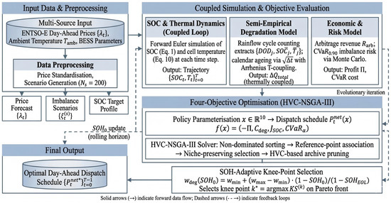
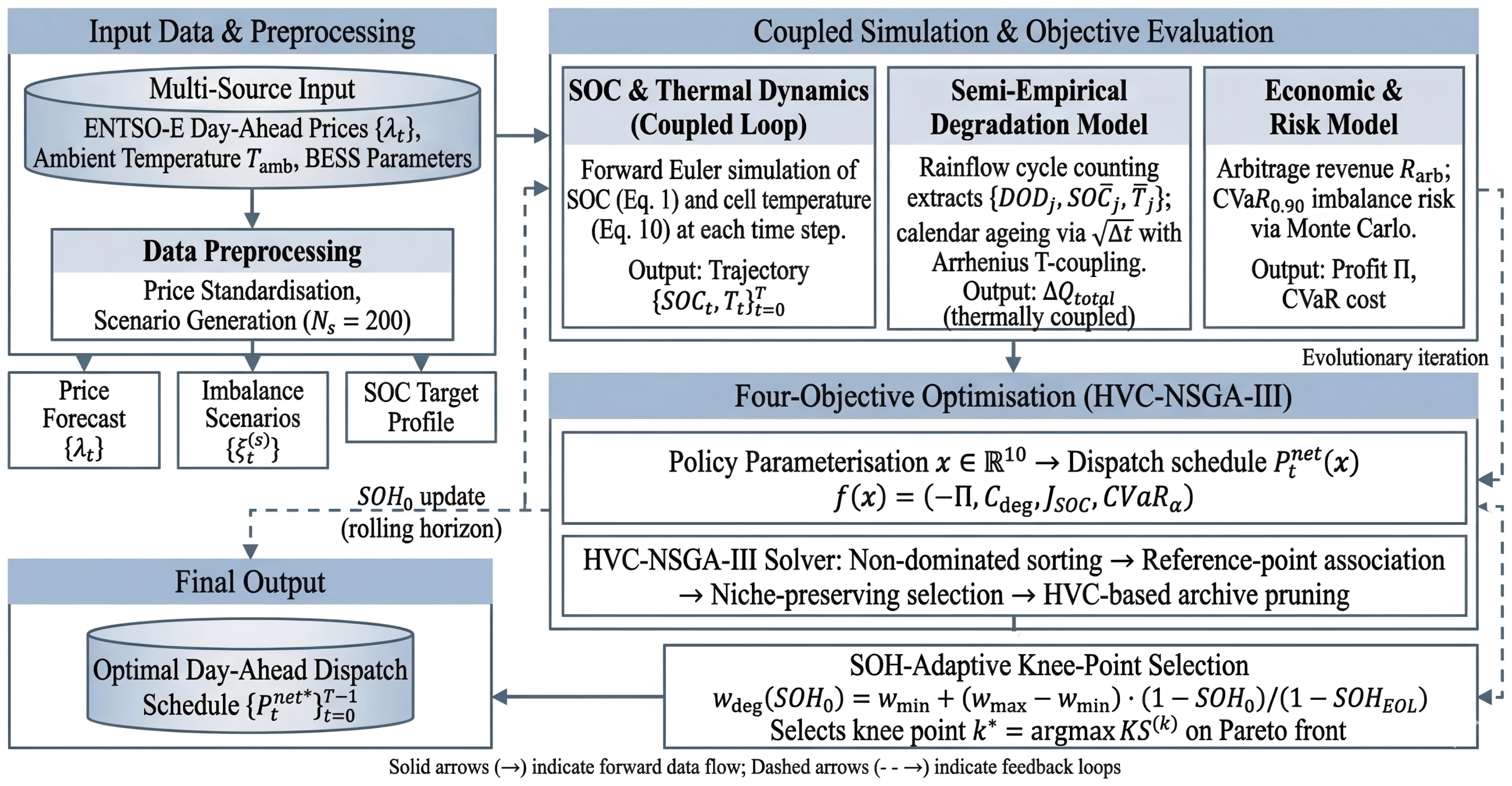
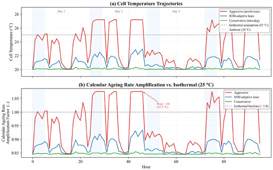
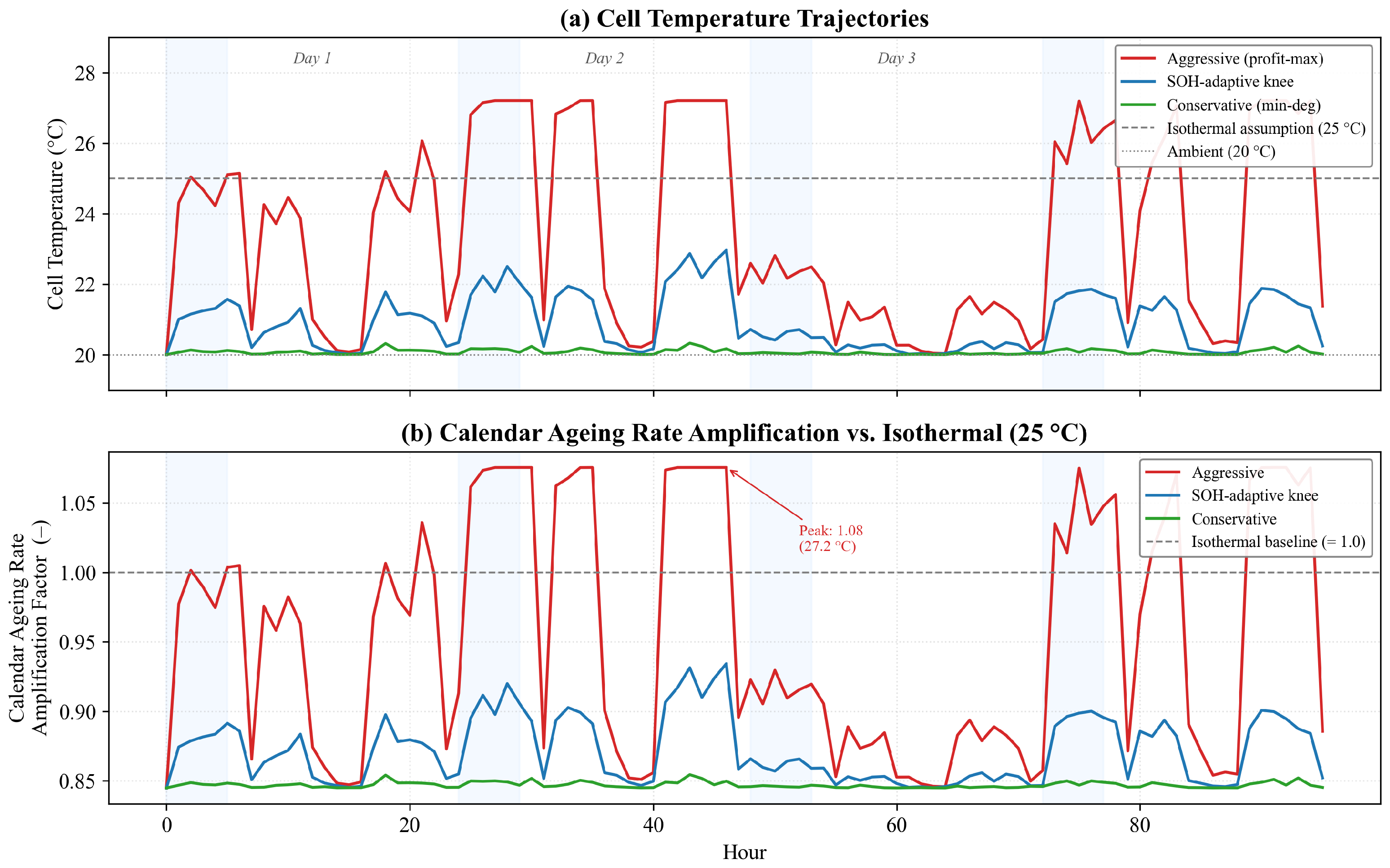
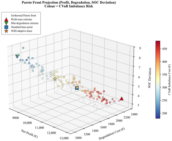
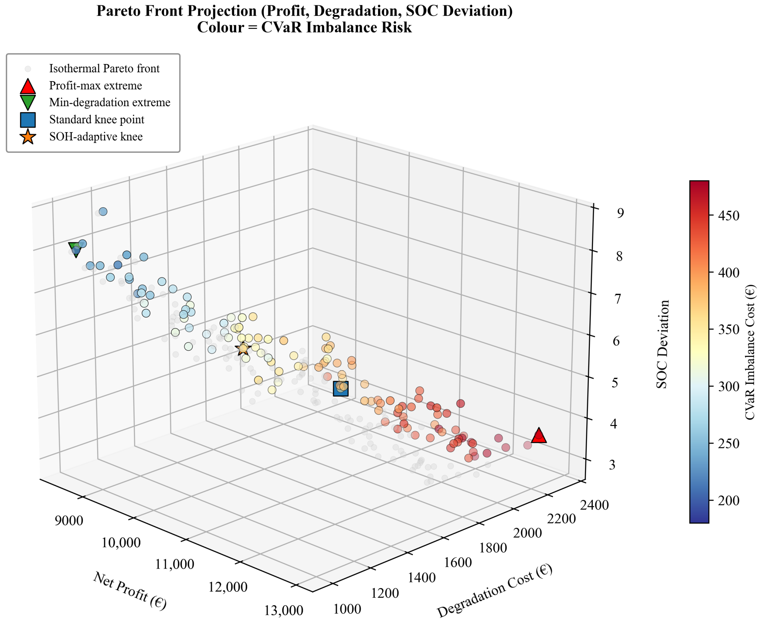
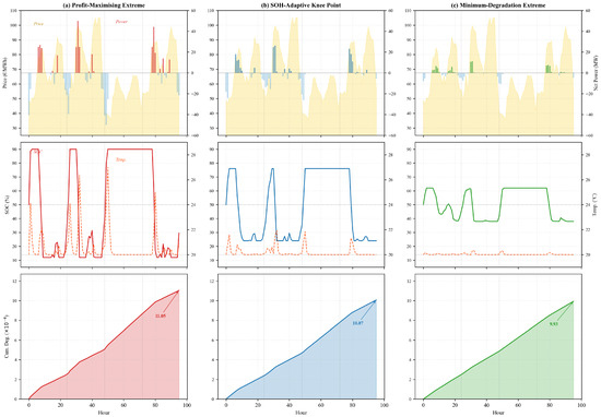
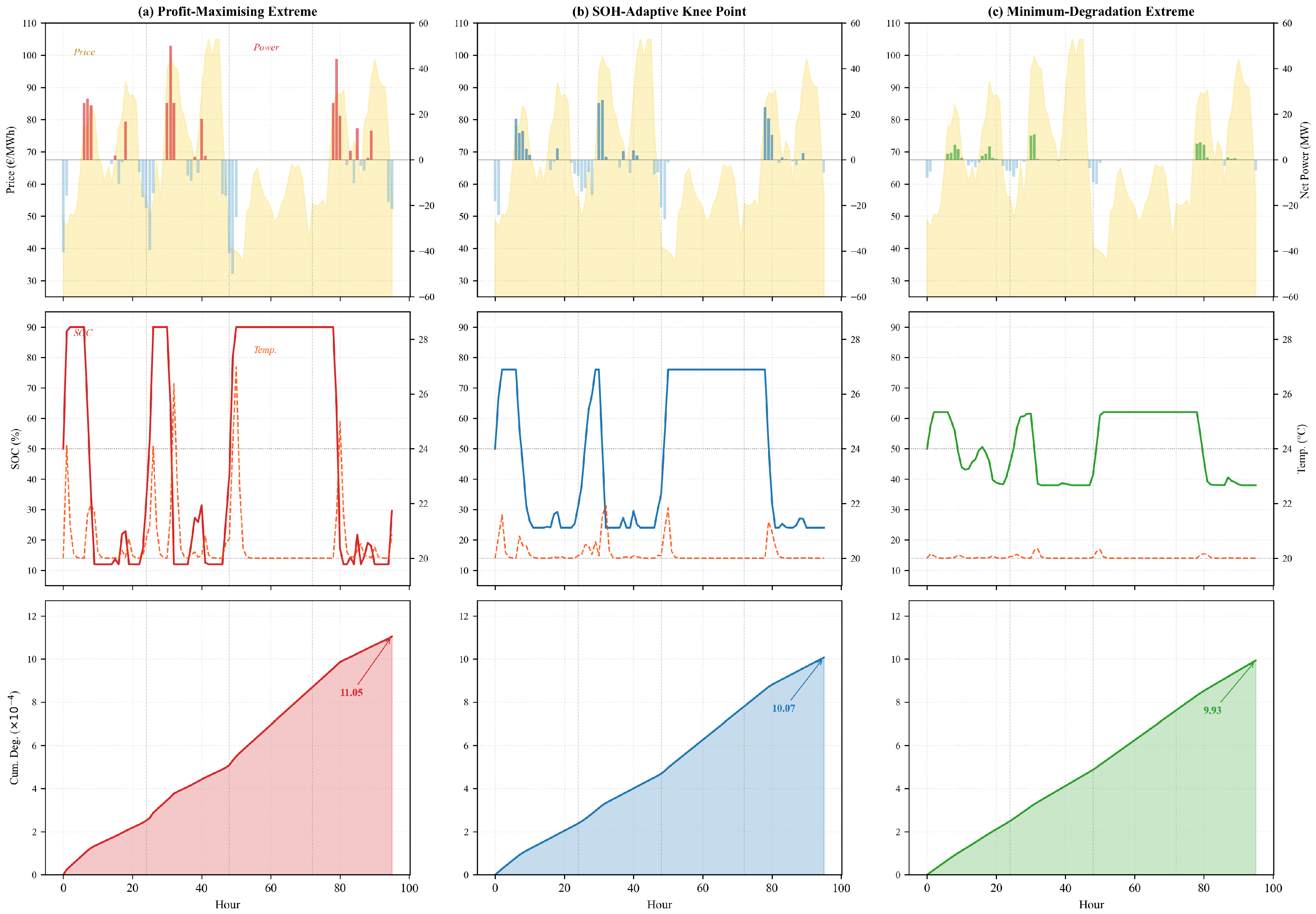
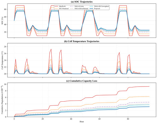
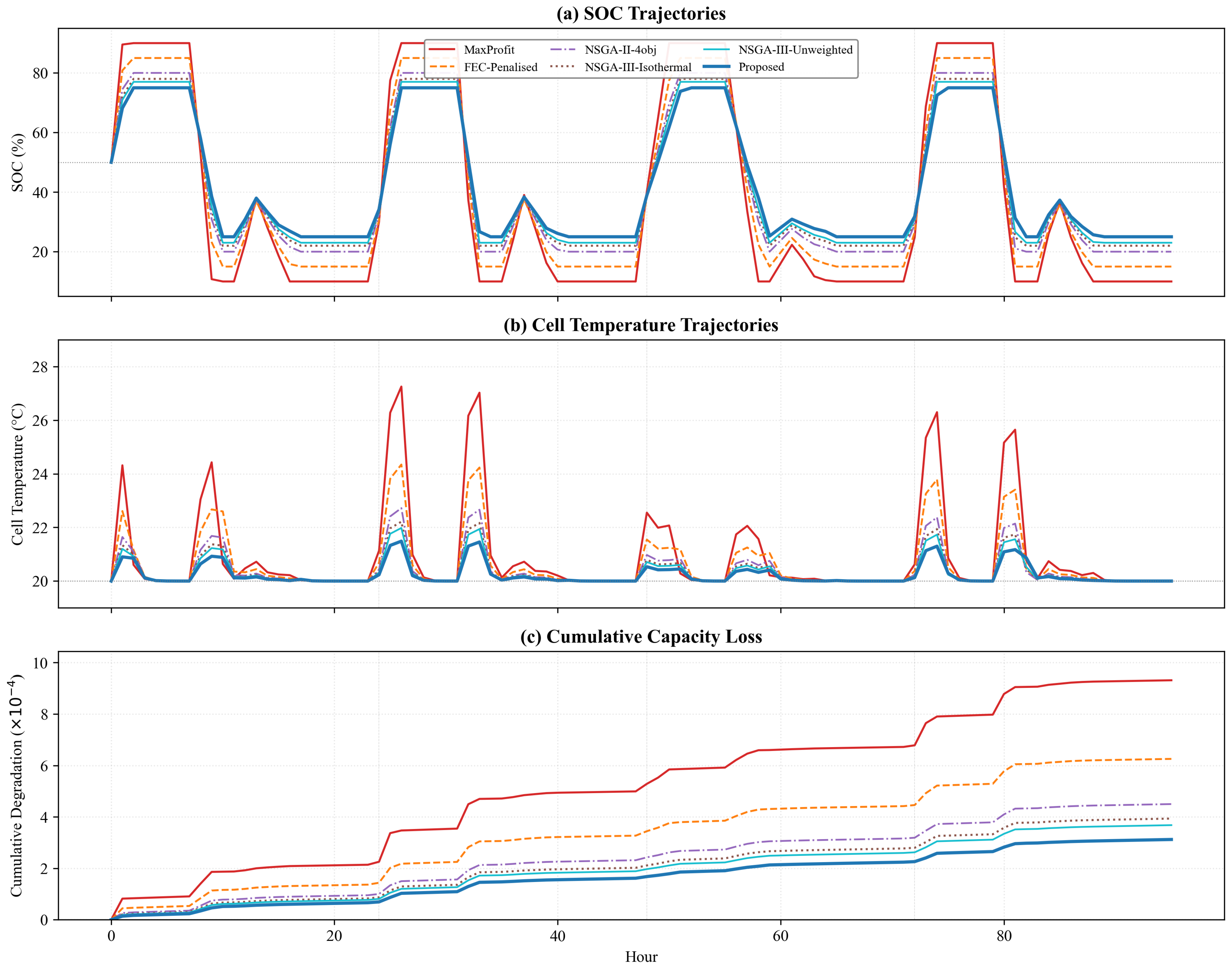
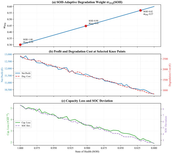
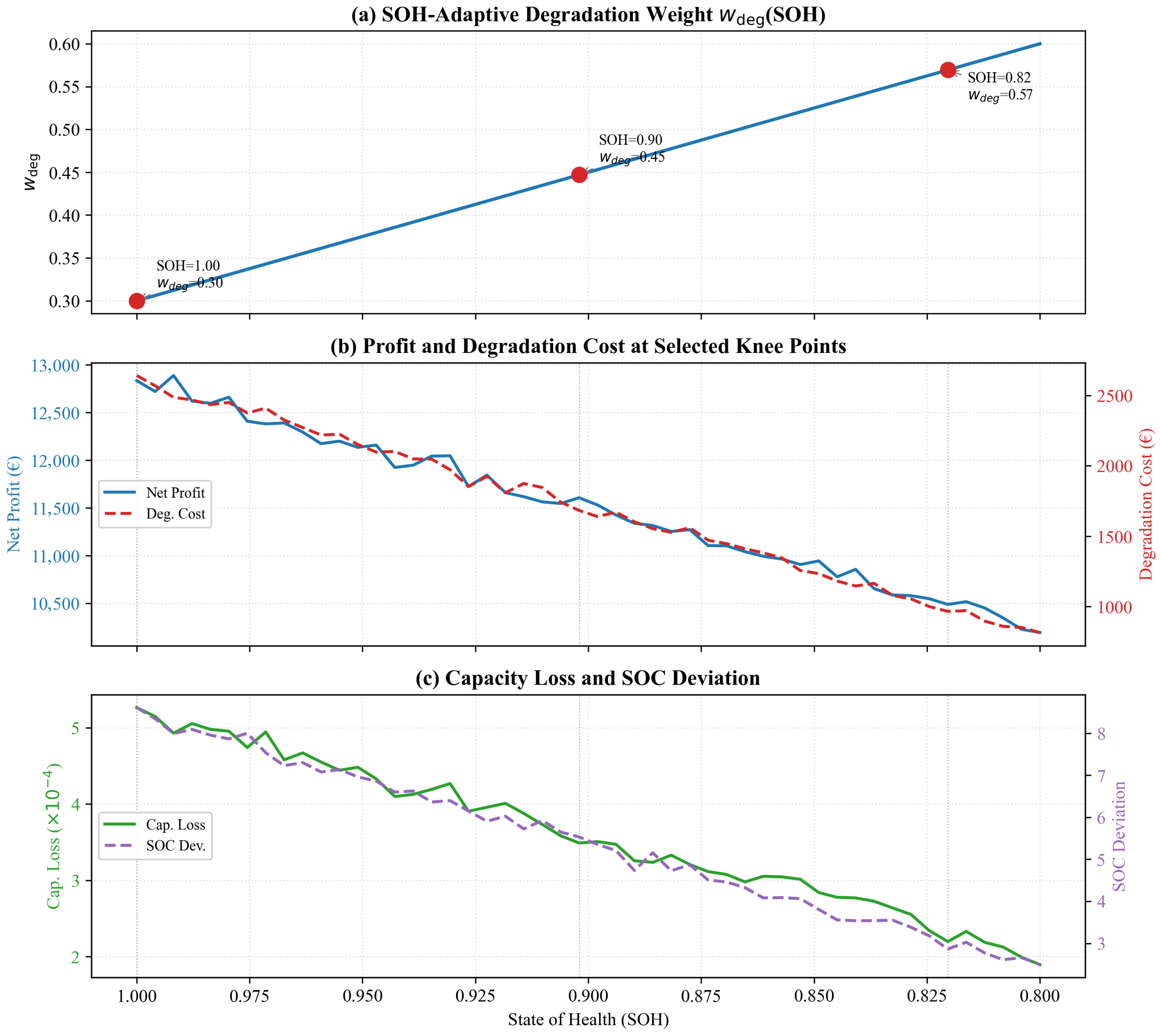
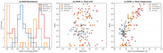
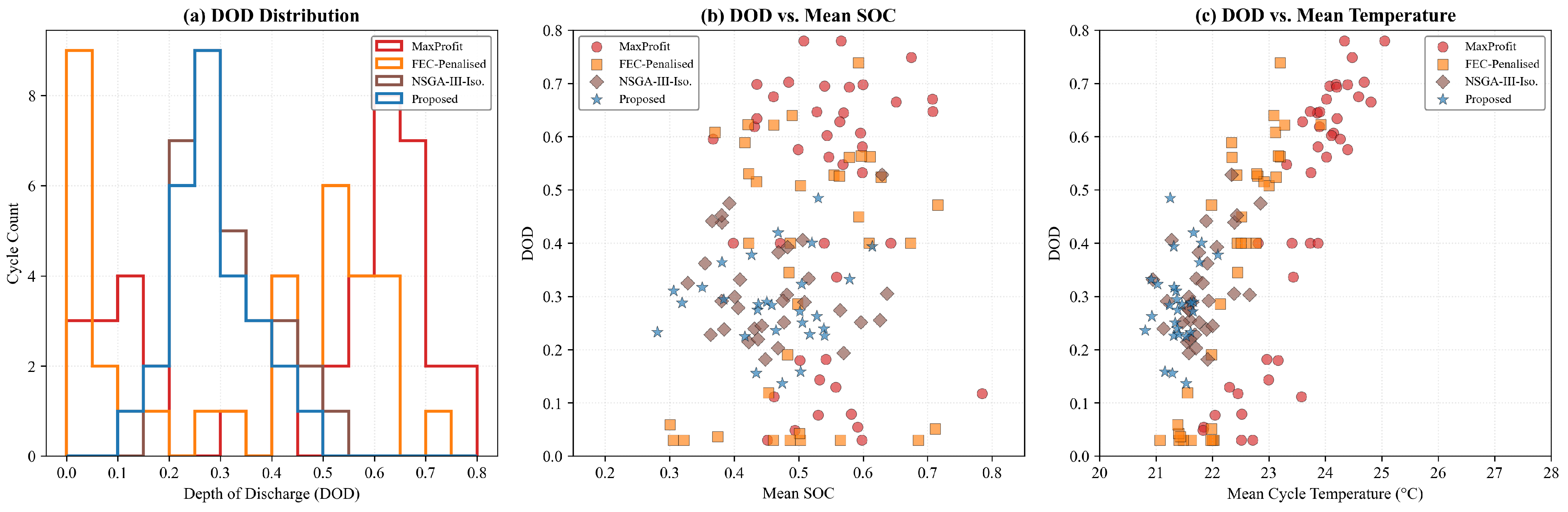
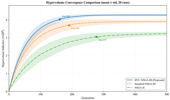
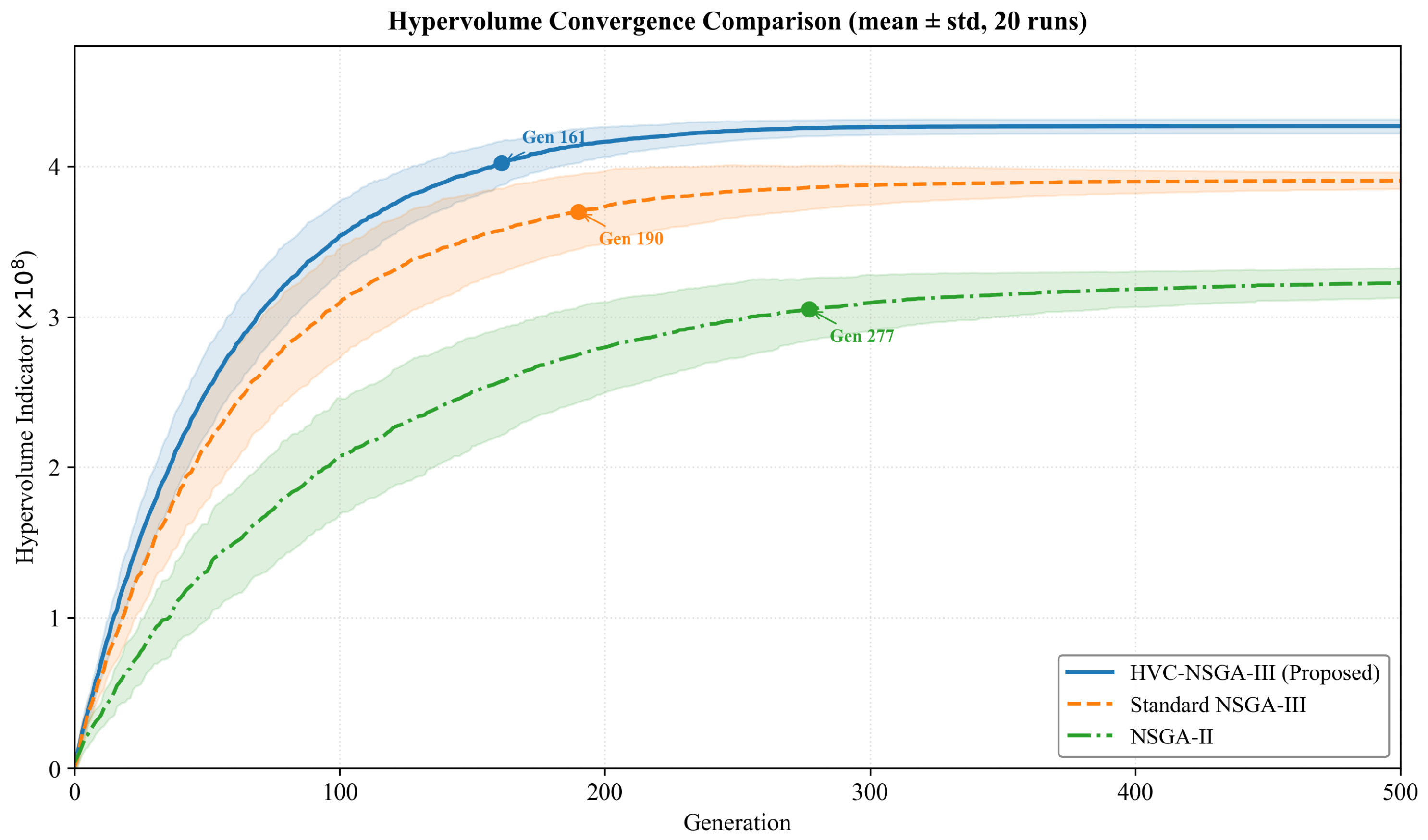

Disclaimer/Publisher’s Note: The statements, opinions and data contained in all publications are solely those of the individual author(s) and contributor(s) and not of MDPI and/or the editor(s). MDPI and/or the editor(s) disclaim responsibility for any injury to people or property resulting from any ideas, methods, instructions or products referred to in the content. |
© 2026 by the authors. Licensee MDPI, Basel, Switzerland. This article is an open access article distributed under the terms and conditions of the Creative Commons Attribution (CC BY) license.