


Abstract
Battery ageing is inevitable during operation, leading not only to performance degradation but to potential safety concerns. Consequently, accurate prediction of the state of health (SOH) of lithium-ion batteries is crucial for ensuring their safety and reliability. This study proposed a novel hybrid neural network architecture that integrates a transformer module, an empirical degradation (ED) model, and a gated recurrent unit (GRU). The transformer module enhances the global representation of the feature sequence, while the ED model comprehensively considers the impact of temperature on the rate of battery capacity degradation, compensating the un-interpretability of the transformer architecture in predicting SOH. In addition, pseudo-incremental capacity curves have been obtained using charging fragments from multi-stage constant current fast charging, which solves the issue of extracting mechanism features under fast charging conditions. Experimental results demonstrate that, across a wide temperature range, the model maintains a low average RMSE between 0.43% and 0.59% for prediction horizons of 4 to 128 cycles. Specifically, the average RMSE is 0.87% at −5 °C and 0.37% between 25 °C and 55 °C. Compared to standalone data-driven models, the proposed hybrid architecture reduces prediction error by approximately 50% at 25 °C, exhibiting superior predictive performance and robustness.
1. Introduction
Energy-saving and environmentally friendly lithium-ion batteries are widely adopted as the power source for electric vehicles and energy storage systems due to their numerous advantages, such as high energy and power density, long cycle life, and low self-discharge rate. However, during prolonged use, beyond the normal chemical reaction of lithium ions intercalating and de-intercalating at the positive and negative electrodes, irreversible damage often occurs. This includes the thickening of the solid electrolyte interphase (SEI) film and/or lithium plating and the degradation of electrode materials [1], ultimately leading to varying degrees of aging in lithium-ion power batteries [2]. The direct consequences of lithium-ion battery aging include capacity degradation, power reduction [3], and the risk of thermal runaway, which directly affects the range, performance, and safety of electric vehicles. Therefore, research on the capacity degradation prediction of lithium-ion batteries enables the assessment of their operational condition, thereby providing assurance to reduce equipment maintenance costs and enhance system operational reliability.
Monitoring the state of health (SOH) of lithium-ion batteries is critical for the safe and reliable operation of energy storage systems. The SOH of batteries depends on the battery aging mode and is influenced by multiple factors, both of which pose challenges for accurate SOH estimation. Model-based approaches utilize either equivalent circuit models (ECMs) [4,5,6] or electrochemical models (EMs) [7,8] to predict battery behavior. While these methods offer theoretical insights, the complexity of internal battery reactions, the diversity of data noise, and a deep understanding of electrochemical mechanisms undoubtedly increase the difficulty of battery SOH estimation [9].
Data-driven SOH estimation models can study the relationship between external measurement parameters and internal state without delving into complex battery principles [10]. The SOH of the battery is typically estimated from parameters extracted from measurable signals, such as battery voltage, current, and temperature, when using battery capacity to characterize battery health. Severson [11] extracted physical features from a battery’s operating current, voltage, and temperature data using discharge voltage curves from the first 100 cycles. They then established the relationship between these features and battery lifespan using regularized regression to predict cycle life. However, this method requires the battery to be fully discharged (discharged to the cut-off voltage), which is difficult to achieve in practice. Richardson [12] proposed a method for estimating battery capacity using Gaussian Process Regression (GPR). This method employs a partial charge voltage segment lasting 1450 s (at a current rate of 1 C, starting from 3.7 V), achieving an estimated root mean square error of less than 3%. He [13] estimated battery capacity degradation using peak intensity reduction, position shift, and the area of the incremental capacity (IC) curve or differential voltage (DV) duration. Tagade [14] proposed a deep GPR architecture that bypasses the input feature extraction stage, directly employing partial charge–discharge time series data for capacity estimation. Three-dimensional data, including voltage, temperature, and time, is randomly selected from charge or discharge curves.
In recent years, research has gradually expanded from “capacity/SOH point estimation” to the prediction of capacity degradation trajectories, which involves forecasting the complete path of capacity evolution over cycles based on historical operating data, so as to better support maintenance decision-making and life management. Early-stage trajectory prediction is one of the earliest research threads in this direction, with its core objective being the reliable extrapolation of subsequent degradation evolution using only a limited amount of early-cycle data [15]. Building upon this, the deep learning approach further proposes a one-shot trajectory prediction framework, which can directly output the future capacity degradation trajectory without the need for iterative rolling predictions and estimate key life events such as the knee point and the end-of-life (EOL) point [16]. Subsequently, to address complex varying operating conditions and differences in life stages, some studies have proposed generalizable trajectory prediction methods applicable to different life stages. These methods utilize charging data from any given stage to construct key points and reconstruct the degradation trajectory through interpolation/extrapolation, thereby enhancing applicability under complex aging conditions [17]. Furthermore, targeting real-world vehicle scenarios, other studies have employed stochastic degradation processes to model capacity evolution, achieving trajectory prediction while emphasizing engineering applicability [18].
Despite advancements in the predicted capacity degradation trajectories made by the aforementioned methods, a single data-driven model still struggles to consistently learn the degradation characteristics under different aging mechanisms when subjected to wide temperature ranges and diverse operating conditions. Particularly during accelerated degradation phases triggered by mechanism changes, such as lithium plating under low-temperature conditions, there remains room for improvement in the model’s interpretability, reproducibility, and consistency in multi-horizon trajectory prediction. In existing research, deep learning-based estimations of SOH/capacity fade widely employ CNN, RNN, Transformer, or their hybrid architectures [19] to learn the degradation mapping from signals such as voltage, current, temperature, or IC. However, under wide temperature ranges and diverse operating conditions, these methods still face issues such as insufficient generalization capability, as well as weak interpretability and reproducibility. Compared with existing methods such as life-stage interpolation/extrapolation, stochastic degradation processes, and one-shot/early-stage pure data-driven trajectory prediction, the main novelty and advantages of this paper lie in the following: It proposes a model architecture that couples an empirical degradation (ED) prior with a deep learning model, enabling capacity degradation trajectory prediction across multi-horizon spans of 4–128 cycles. Furthermore, it constructs reconstructed V-Q sequence features from multi-stage constant current fast-charging data, achieving effective extraction of mechanism information under fast charging conditions.
The remainder of this paper is organized to systematically present the research workflow. Section 2 begins by describing the multi-stress aging test campaign conducted under various temperatures and operational profiles to generate the necessary degradation data. Building upon this experimental foundation, Section 3 elaborates on the feature extraction process, particularly from the IC curves, and details the novel architecture of the proposed empirical degradation-guided Transformer–GRU (TGRU) model. Concluding the study, Section 4 offers a mechanistic analysis of the observed battery degradation and presents a thorough evaluation of the model’s predictive accuracy and generalization capability across different conditions.
2. Batteries Datasets
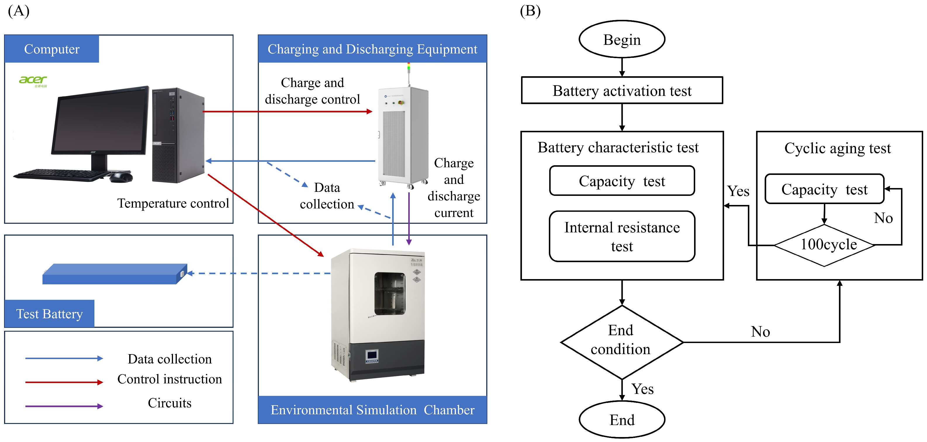
To establish a wide-temperature-range and multiple-working-condition battery-capacity-degradation dataset, a commercial 198 Ah prismatic power battery (LFP/Graphite) was adopted as the research subject. The cell-level lithium-ion power battery test platform used in this study is shown in Figure 1A. This test platform primarily consists of four components: a charge/discharge testing device that controls the charge/discharge current with ±0.02% F.S. voltage accuracy and ±0.03% F.S. current accuracy, produced by XingYun Electronics Co., Fuzhou, Fujian, China; a temperature test chamber that regulates the battery’s ambient temperature, produced by Bell Equipment Co., Huizhou, Guangdong, China, with 0.1 °C temperature accuracy; a computer for data storage and programming; and the battery samples. The measurement range and acquisition accuracy of all test equipment met the experimental requirements.
Figure 1.
(A) Schematic diagram of the test platform for a lithium-ion battery at the cell level. (B) Flowchart of lithium-ion battery test.
The testing process for lithium-ion power batteries, as shown in Figure 1B, primarily consisted of three major stages: the battery wake-up test, the cycle aging test, and the battery characteristic test. The battery life aging test was conducted at room temperature. The experimental process was as follows: the batteries were charged with a multi-stage constant current charging system provided by the manufacturer until their voltage reached the upper cut-off value of 3.8 V, followed by a constant voltage stage till the current was below 0.05 C; then, the batteries were discharged with a constant current of 200 A to a voltage of 2.0 V.
The battery cycle aging test conditions are shown in Table 1, primarily comprising cell cycle tests under different charging rates. Taking the temperature rise and the possibility of lithium plating at −5 °C and of the generation of gas at 55 °C into account, the charging rate at −5 °C and 55 °C was appropriately reduced.
Table 1.
Battery aging experimental conditions.
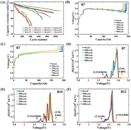
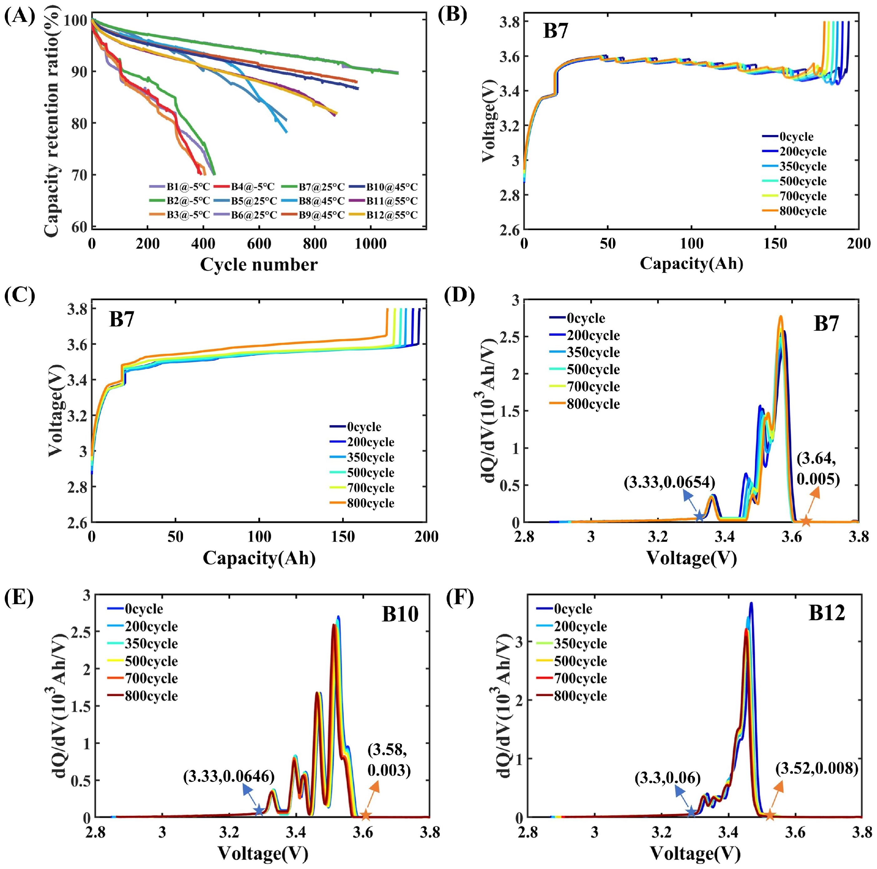
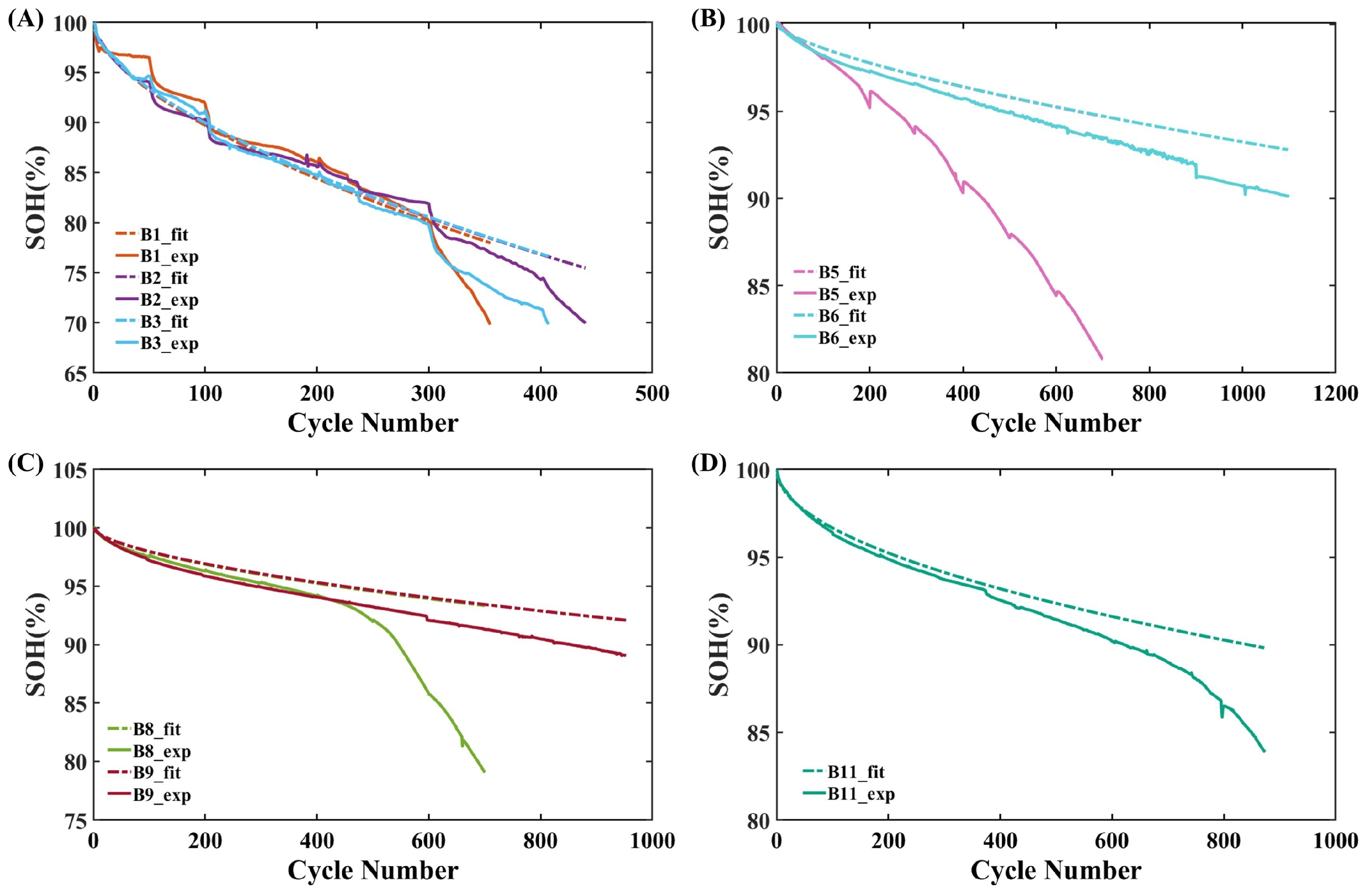
CC denotes constant current charging, DC denotes constant current discharging, MCC denotes multi-stage constant current charging, and 1.6 C (MCC) denotes a multi-stage constant current charging mode equivalent to 1.6 C. The detailed current and voltage for MCC is shown in Figure A1. Battery characteristic testing primarily aims to obtain the characteristic parameters of cells under different aging states. This testing includes capacity calibration tests, direct current internal resistance (DCR) tests, and low-current tests. Capacity calibration tests mainly determine the usable capacity of batteries at various aging stages to identify capacity degradation trends. These tests must be repeated three times, with the average of the three measurements representing the usable capacity of the tested battery in its current state, thereby minimizing measurement errors. DCR testing primarily determines the impedance characteristics of batteries at various aging states. All the test schedules for cycle tests and capacity tests are shown in Table A1. The capacity degradation curves of all battery samples are shown in Figure 2A.
Figure 2.
Details of the dataset: (A) capacity retention ratio (every cycle) of all battery samples; (B) cycling voltage curves of B7; (C) reconstructed cycling voltage curves of B7; (D) pseudo-IC curves of B7; (E) pseudo-IC curves of B10; (F) pseudo-IC curves of B12.
3. Methodology
3.1. Feature Extraction
3.1.1. Charging Fragment Selection
The charging curve reflects the degradation characteristics of the battery’s dynamic performance. The IC curve derived from the charging curve typically also reveals the mechanism of internal material loss within the battery, providing consistent input for extracting features of battery aging [20]. However, in practical applications, charging protocols are rarely simple constant-current charging, and charging to full capacity is uncommon, making it difficult to obtain complete charging curves. To better align with real-world scenarios, a method based on IC analysis was adopted. This approach examines the characteristics reflected in complete charging data to select charging segments that encompass aging features related to material loss, lithium inventory loss, and kinetic loss in batteries.
In the experimental data presented here, the charging protocols at 25 °C, 45 °C, and 55 °C all employed a multi-stage constant-current charging scheme provided by the battery manufacturer. With up to 11 current switching points, the resulting charging voltage curves deviated from the typical monotonic ascending pattern (as shown in Figure 2B), posing significant challenges for obtaining the battery’s IC curve. To address this issue, this paper adopted the voltage interval partitioning method based on time-equal allocation proposed in the literature [21]. This method first divides the charging voltage segments into voltage bins at fixed intervals. It then calculates the duration the battery spends in each voltage bin. The durations in each voltage bin are subsequently summed to generate a monotonic pseudo “voltage-time” curve. Finally, the corresponding charge quantities for each voltage bin are accumulated to reconstruct the battery’s voltage-capacity (V-Q) curve. Typically, the voltage interval for voltage compartmentalization is set to 1 mV. The reconstructed battery V-Q curve exhibited a monotonically increasing trend (as shown in Figure 2C). It can be observed that the V-Q curve changed from non-monotonic to monotonic after reconstruction. By applying the differentiation process as shown in Equation (1), the pseudo-IC curves presented in Figure 2D–F for different batteries were be obtained. Although the reconstructed V-Q curve was monotonically increasing, it still exhibited several jumps, which resulted from random jumps in the corresponding current between 1 C and 2.3 C after reconstruction.
The pseudo-IC curve of the battery was obtained based on the reconstruction of the V-Q curve described above. As shown in Figure 2D, the number and position distributions of IC peaks on the curve exhibited significant variation due to the influence of charging ambient temperature and charging mode. Simultaneously, as the battery aged, the overall trend across all battery IC curves showed a shift of the main peak position to the right, accompanied by a decrease in peak height and peak area. This indicates that the battery suffered from both thermodynamic and kinetic losses. Specifically, as temperature increased, the ohmic impedance and polarization impedance inside the battery decreased, resulting in a slight shift of the characteristic peaks of the IC curve toward lower voltages, along with an increase in peak intensity. From the perspective of degradation mechanisms, losses occur in both the active materials and the lithium inventory. Specifically, lithium metal plating during low-temperature charging accelerates the irreversible loss of cyclable lithium inventory. Kinetically, this manifests as increased internal resistance, heightened charging polarization with battery aging, and a gradual reduction in charge capacity [22]. To construct a battery capacity degradation prediction model adaptable to wide temperature ranges and multiple charging protocols, the charging segment data with voltages between 3.33 V and 3.64 V were selected, covering all IC peaks under all operating conditions, and significant features characterizing battery aging and operational variations were extracted.
3.1.2. Health Features Extraction
In this study, the health features were extracted from the reconstructed V-Q curve within the specific voltage window . Following the time-equal allocation method described in Section 3.1.1, the charge capacity was no longer a raw time-series but a discretized sequence indexed by voltage bins. To represent the battery’s degradation, the health feature set was constructed by extracting ten statistical characteristics comprising total capacity, mean, median, standard deviation, variance, minimum, maximum, range, skewness, and kurtosis, along with significant IC peak features derived from the pseudo-IC curve, which was obtained by differentiating the reconstructed V-Q curve.
For each voltage bin , the incremental charge capacity was calculated by summing the charge delivered whenever the measured voltage falls within that bin:
where is the current at time , and is the constant sampling interval, which was set to 1 s in this study. denotes the indicator function. The accumulated capacity sequence for the selected voltage range was then reconstructed by prefix-summing the incremental capacities:
where m represents the total number of 1 mV bins within the aforementioned window.
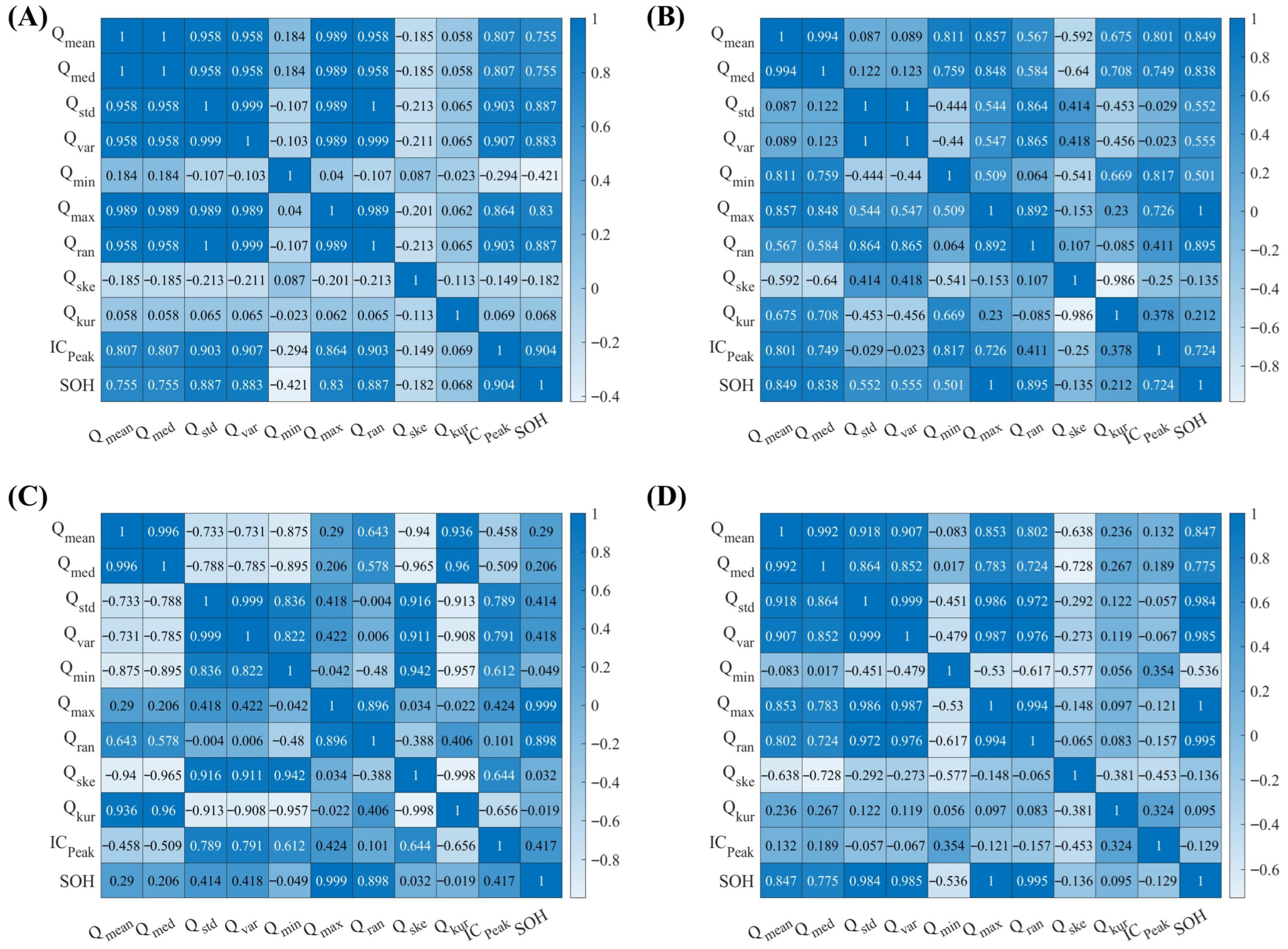
Pearson correlation coefficients between the selected features and battery SOH were calculated separately, with the results of B1 shown in Figure 3. SOH was defined as the ratio of the discharging capacity of a certain cycle to its initial discharging capacity. As shown in Figure 3, at −5 °C, the feature sequences with the highest correlation to SOH were , , , , , , listed in descending order of correlation. During the charging and discharging process of the battery, Li+ repeatedly detaches between the positive and negative electrodes, which is accompanied by side-reactions, resulting in irreversible loss of the chemical substances in the battery. As cycles increase, the side reactions gradually intensify. In the micro view, the SEI will grow, and the electrodes will dissolve. In the macro view, the internal resistance will increase, and the capacity will decrease [23].
Figure 3.
Correlation analysis between each feature and battery capacity of (A) B1, (B) B6, (C) B9, (D) B11.
Figure 3 shows the correlation analysis between each feature and the battery capacity of other batteries. At 25 °C, , , , , exhibited high correlation with battery SOH. At 45 °C, only and showed high correlation with battery SOH; , had moderate relevance. At 55 °C, up to seven features exhibited high correlation with battery SOH: , , , , , . Although IC peak features were extracted for physical analysis, they were excluded from the final input set due to their sensitivity to noise. Therefore, to ensure feature non-redundancy, , , , and were selected as the primary features for input into the battery capacity degradation prediction model.
In addition, since battery aging trajectories vary with operating conditions such as temperature and charge rate, the mean charging current and mean temperature were incorporated to characterize condition-dependent differences. Moreover, the cycle number was included as a degradation-progress indicator to encode usage history and cumulative aging. Notably, both and were also required in the empirical model to account for the cycle-dependent trend and temperature dependence of capacity degradation. Ultimately, these features collectively constituted the input for the battery capacity deterioration prediction model. The features encompass operating-condition and aging-progress metrics, , and , alongside statistical features derived from the reconstructed V-Q sequence, including , , , , and .
3.2. Empirical-Degradation-Guided Transformer–GRU Framework
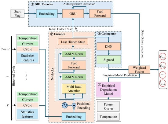
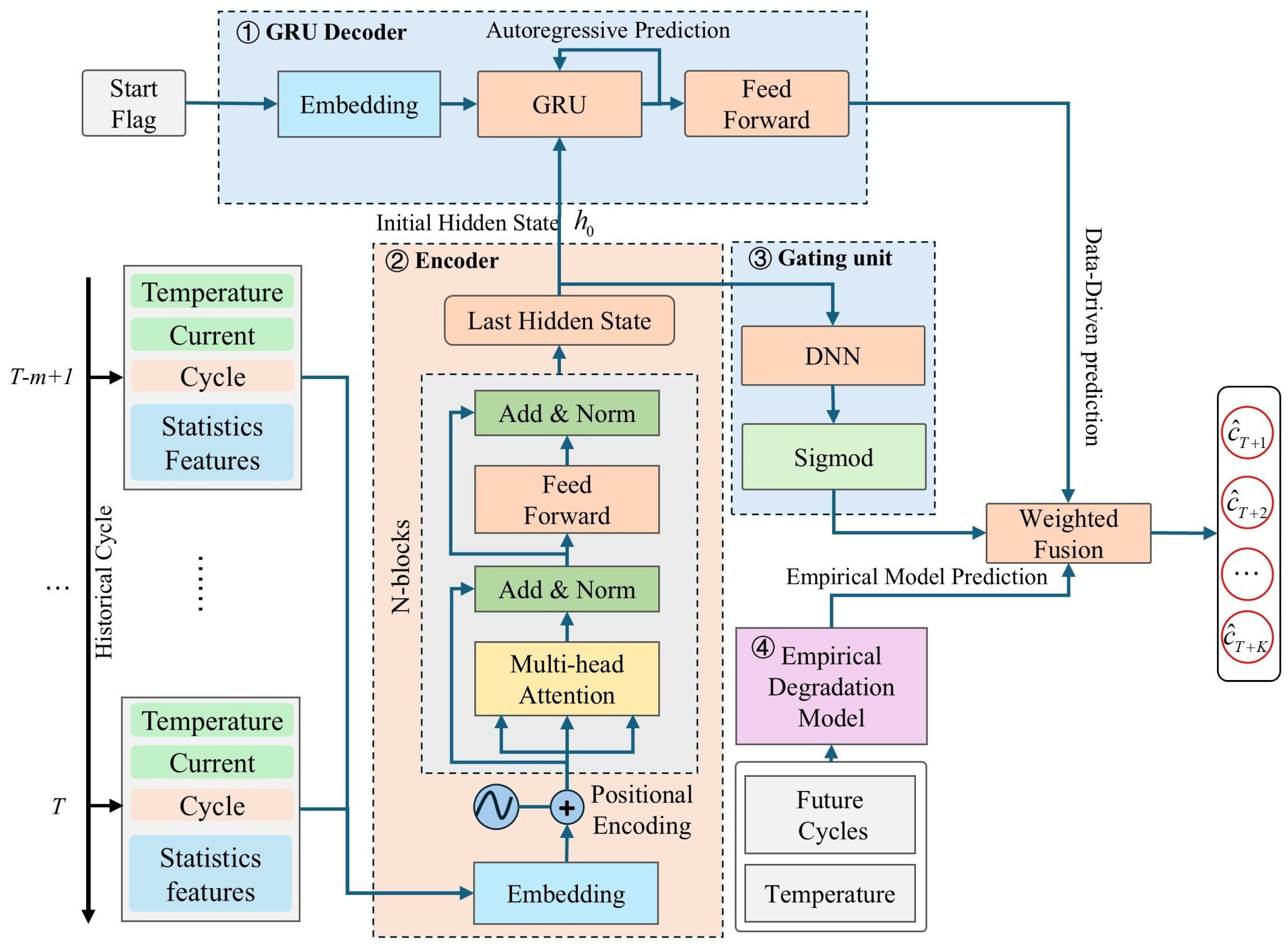
This paper proposes an Empirical Degradation-Guided Transformer–GRU (ED-TGRU) model for predicting the degradation trajectory of battery SOH. The model integrates empirical degradation trend priors with deep sequence modeling, comprising four core components: a Transformer encoder based on self-attention, a GRU decoder, an empirical degradation prior module, and an adaptive fusion gating unit. At the structural design level, the ED-TGRU model first feeds the Transformer encoder with temperature information, cycle count, and statistical features of V-Q curves from historical cycles to capture global degradation trends and long-range dependencies. Subsequently, the GRU’s hidden state is initialized using the encoder’s output features at the final time step, and an SOH degradation sequence is generated via autoregressive prediction. To enhance prediction stability, the ED-TGRU model incorporates an empirical degradation model as a trend prior and dynamically fuses GRU predictions with the empirical model’s output via an adaptive gating mechanism. The overall structural diagram of this model is shown in Figure 4.
Figure 4.
A schematic diagram of the overall structure of the ED-TGRU model.
3.2.1. Transformer Encoder
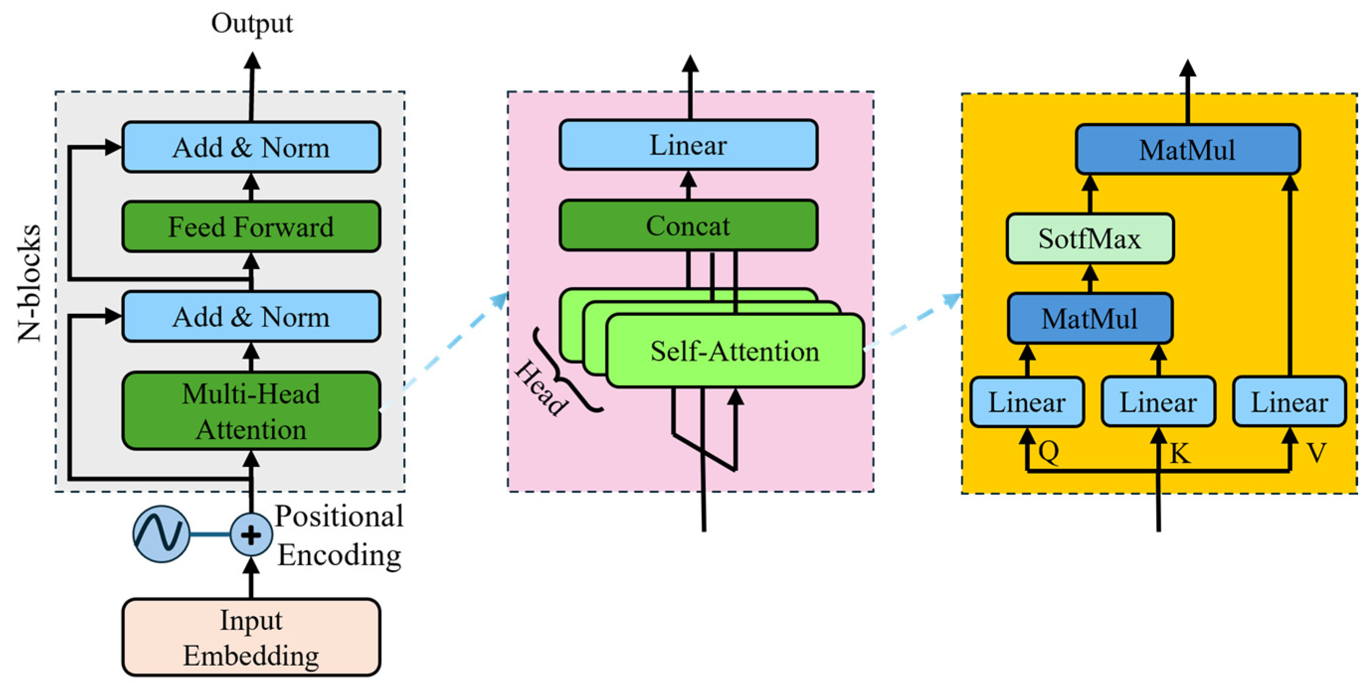
The standard Transformer uses a sequence-to-sequence framework comprising an encoder and a decoder. The encoder analyzes the input sequence and produces high-dimensional representations, which are subsequently transmitted to the decoder to generate the output sequence [24]. The Transformer, originally designed for natural language processing, has demonstrated exceptional efficacy in other fields owing to its robust sequence modeling capabilities, including tasks involving residual useful life prediction [25]. For battery state-of-health prediction tasks, we utilized the Transformer encoder’s self-attention mechanism to capture global dependencies in the input data, thereby abstracting semantically rich aging aspects. The Transformer encoder module is utilized to extract degenerate features from the input sequence. It has M identical sublayers, each comprising two components: a multi-head self-attention module and a feedforward module, as seen in Figure 5.
Figure 5.
Transformer encoder.
To model the feature sequences from the input encoder and extract information-dense representations, the aging feature vector obtained from each charge segment is first embedded via an embedding matrix into a -dimensional vector representation. Relative position encoding is subsequently applied to this vector. After position encoding, the output at position is denoted as:
where denotes the current cycle number of the battery, m denotes the historical cycle number input to the encoder, and the position information code inserted at the - place. The calculation technique is as follows [24]:
where represents the index of the time step, while 2k and 2k + 1 represent the even and odd dimensions of the position encoding, respectively. refers to the model’s embedding dimension.
In the self-attention mechanism, the encoder first linearly transforms the input sequence into query, key, and value vectors. Attention weights are computed by measuring the relationships between query and key vectors, enabling the weighted aggregation of value vectors to capture internal dependencies within the sequence. However, single attention often fails to capture multiple relational patterns simultaneously. Consequently, the Transformer uses a multi-head self-attention mechanism, partitioning the attention computation across several concurrent heads. These heads capture local and global, as well as multi-scale, dependencies across various representation subspaces, thereby augmenting the diversity and resilience of feature representations. The computational procedure for each self-attention head is as follows:
where represents the input to the self-attention module, H signifies the number of parallel attention heads, and ,, are trainable weight matrices, with . The outputs from all attention heads are ultimately concatenated and processed through a linear layer to get the final representation. The mathematical formulation for multi-head self-attention is as follows:
where represents trainable parameters, and denotes the concatenation function.
After completing the self-attention computation, the encoder applies residual connections and layer normalization to the output. It is subsequently processed by a positional feedforward network, yielding a complete encoder layer. Stacking multiple encoder layers produces an encoder output sequence that corresponds in length to the input sequence, with each position’s feature representation incorporating comprehensive dependency information, as illustrated below:
3.2.2. GRU Decoder
GRU is an effective variant of recurrent neural networks that enables the selective regulation of information flow through reset and update gates, thereby alleviating the vanishing gradient issue characteristic of conventional RNNs to some degree [26]. In this paper, a GRU was used as a decoder to generate SOH trajectories via autoregressive inference. This method provides superior computational efficiency, a more streamlined architecture, mitigates overfitting, and improves the model’s generalization performance compared with a Transformer decoder with masked self-attention. The forward calculation process for the GRU is as follows:
where signifies vector concatenation, indicates element-wise multiplication, and denotes the Sigmoid function; represents the decoder input at time step ; denotes the GRU hidden state at time step ; and are the reset gate and update gate, respectively; signifies the candidate hidden state; and are learnable parameters. As the update gate nears 0, the model is inclined to preserve more historical hidden states; conversely, as approaches 1, it increasingly favors the candidate hidden state produced at the current time step. The GRU dynamically balances the interplay between past data and current input, enabling resilient sequence modeling. The concealed characteristics produced by the GRU network, after traversing a fully connected layer, generate the capacity prediction value for the forthcoming time step, as illustrated below:
Based on the forward computation of the GRU unit, the initial hidden state in the GRU-based decoder sets the initial conditions for subsequent hidden state updates, thereby influencing the generation of the output sequence. Consequently, its selection is vital to the accuracy of capacity prediction outcomes. Given that battery SOH degradation exhibits temporally accumulated and predominantly monotonic behavior, and that the terminal time-step feature produced by the encoder aggregates degradation information over the entire historical input sequence, this paper adopts it as a compact summary of historical operating conditions and degradation status. Considering the consistency between future and historical operating states, along with the cumulative effects of internal aging, this paper employs the encoder’s terminal feature to initialize the GRU hidden state and updates it recursively with a constant starting label . This enables the model to learn intrinsic degradation dynamics and predict future capacity changes accordingly. The decoder forecasts the capacity degradation trajectory for the next K steps through the following recursive relationship:
where denotes the predicted value for the capacity at the k- future step, and represents the decoder’s hidden state at the corresponding time step.
3.2.3. Empirical Degradation (ED) Model
Capacity is another key parameter for evaluating battery performance. When describing the capacity decay pattern of lithium-ion batteries, the curve showing the change in discharge capacity per cycle over the number of cycles during battery aging is typically used, as shown in Figure 2A. The battery capacity can often exhibit a two-stage degradation process: an initial linear decline followed by an exponential acceleration toward the end of its lifespan. This degradation pattern suggests that, during the early usage phase, the battery may experience a relatively stable performance decline due to a “break-in” effect. However, in the later stages, material fatigue, accumulated damage, and potential irreversible electrochemical changes lead to a sharp capacity loss. Under different test conditions, the capacity decay curves of batteries exhibit significant differences from the outset. This phenomenon may be attributed to variations in temperature and charging strategies altering the thermodynamic decay rate of the batteries.
Differences in battery capacity decay rates at varying temperatures indicate that temperature can alter the rate of battery chemical reactions. However, it does not change the type of random degradation process or the functional form of the degradation equation. Based on this, overall battery capacity decay under thermal stress still follows a Gaussian process. The relationship between battery SOH and cycle count at different temperatures is expressed as follows:
where represents the initial capacity of the battery, T denotes Kelvin temperature, indicates the number of cycles, is the reaction rate, and is a temperature-dependent expression.
Equation (11) quantitatively describes the effect of temperature on battery capacity decay and thus can be defined as a degradation equation. represents the rate of the chemical reaction, conforming to the three-parameter modified Arrhenius equation. can be expressed as a binomial term, thereby formulating the battery SOH expression as follows:
where a, b, c, d, e, f are pending parameters.
3.2.4. Dynamic Gating Fusion Mechanism
A dynamic gating mechanism is used to adaptively balance the contributions of the empirical degradation model and the Transformer–GRU model, thereby optimizing the application of the physical laws governing battery degradation while maintaining the data-driven model’s capacity to identify intricate patterns. A gating parameter is introduced, with its weight adaptively generated from the global sequence features recovered by the encoder from previous input sequences. This illustrates the general pattern of deterioration and stabilizes the empirical degradation model’s contribution to forecasts. The gating weight is computed as follows:
where and are trainable weight matrices. The ultimate prediction is a weighted combination of the outcomes from the empirical degradation model and the ED-TGRU model:
As approaches 0, the model predominantly uses empirical degradation models to maintain reasonable predictive performance; as approaches 1, the model increasingly relies on data-driven features to capture intricate or non-ideal degradation patterns. This gating mechanism allows the model to deliver dependable degradation trend guidance via empirical degradation models while adaptively modifying weights when the Transformer–GRU model identifies complex patterns, thereby improving predictive stability and robustness across varying operating conditions.
4. Discussion
4.1. Evaluation Indicator
The end of life for data partitioning is defined when the battery state of health (SOH) declines to 70%, serving as the uniform cut-off criterion for the cycle data of all batteries. A total of 12 battery samples was selected for model training and test sets. To evaluate the model’s generalization performance under different temperature conditions, one battery from each temperature range was chosen as a test sample. Specifically, “B4”, “B7”, “B10”, and “B12” were designated as the test set to independently evaluate the prediction accuracy and stability of the model under various operating conditions. This data partitioning strategy ensures the diversity of the training data and the comparability of test results, providing a solid foundation for reliably evaluating the ED-TGRU model in modeling battery degradation processes.
To accurately measure the performance of the battery capacity fade prediction model, three indexes of mean squared error (MSE), mean absolute error (MAE), and root mean squared error (RMSE) were adopted as evaluation metrics for battery capacity estimation. These metrics were used to assess the overall deviation level of the capacity fade prediction model and the estimation deviation under the worst-case scenarios.
where and represent the measured and predicted values of the - SOH observation, respectively, and denotes the total number of samples.
4.2. Parameters Identify and Results of ED Model
To assess the prediction performance of the ED model, the model parameters were first determined by the least squares method utilizing training set data. The ED model is delineated in Equation (13), wherein the cyclic input consists of the mean temperature sequence within the specified voltage range and the associated number of cycles. Using the identified parameters, the model expression can be written as follows:
The quantitative fitting performance of the ED model on the training set is summarized in Table 2, where the RMSE and the coefficient of determination are calculated for each battery. The fit result of ED models are shown in Figure 6 for the training set.
Table 2.
Quantitative fitting evaluation of the ED model for the training set.
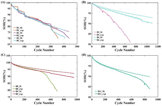
Figure 6.
Fit result of ED model for −5 °C (A), 25 °C (B), 45 °C (The purple dotted line and cyan dotted line almost overlap.) (C), 55 °C (The green dotted line and red dotted line almost overlap.) (D).
The ED model, while physically interpretable, exhibits inherent limitations in capturing complex non-linear aging behaviors even at ambient temperatures. As shown in Table 2, the model displayed significant fitting failures for B5 (25 °C, ) and B8 (45 °C, ). Although the Arrhenius equation is widely used for temperature dependence, it struggles to account for the accelerated capacity decay observed in these cells, which may be triggered by rapid SEI growth or electrode material loss during mid-to-late cycling. Similarly, the ED model couldn’t reflect abnormal degradation mechanisms, such as lithium plating, that occurred at low temperatures for B1, B3 and B4. Consequently, while the ED model maintains high fidelity for cells with linear degradation primarily above 0 °C, its performance diminishes when confronted with the diverse and non-linear aging trajectories of LFP cells. This discrepancy confirms that relying solely on the ED model may introduce systematic errors in SOH prediction under extreme or complex conditions. Therefore, integrating the TGRU network to compensate for these residuals allows the hybrid ED-TGRU model to outperform standalone TGRU or ED models. Even though long-term SOH trajectories for LFP cells are often considered quasi-linear, the ED model alone remains insufficient for capturing the intricate, condition-dependent degradation dynamics required for high-precision forecasting.
4.3. SOH Predicting Results
This study employed a lightweight sequence-to-sequence (Seq2Seq) Transformer model for time series prediction tasks. The model consists of a single encoder layer and a single decoder layer, with a hidden dimension of 32, achieving the efficient modeling of temporal features with a relatively small parameter size. During training, the batch size was set to 64, and the AdamW optimizer was used with an initial learning rate of 0.001. This model structure is concise and exhibits stable training, effectively reducing computational complexity while maintaining prediction accuracy, making it suitable for tasks such as battery state of health estimation and capacity degradation trend prediction.
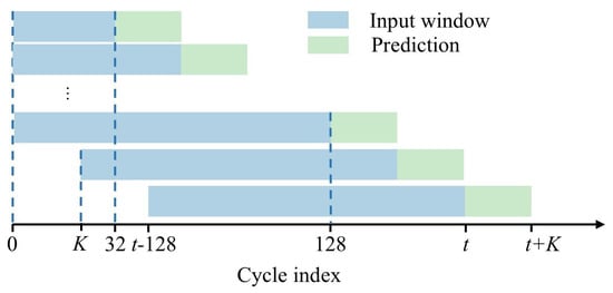
The model input adopts a variable-length sequence design, with a minimum length of 32 and a maximum length of 128, to adequately capture the historical information characteristics of different batteries at various stages. Through its self-attention mechanism, the Transformer can flexibly model global dependencies between different time steps in a sequence. Consequently, when faced with variable-length inputs, it can adaptively focus on key degradation features without requiring a fixed time window. During training and prediction, the input and target sequences were divided as shown in the figure below.
For the prediction task, targeting different stages of the battery degradation process, the model employs three prediction schemes: short-term degradation trend prediction for the next 4 cycles, used to capture local fluctuations and short-term anomalies; medium-term degradation trend prediction for the next 32 cycles, used to characterize the overall decay trajectory; and long-term degradation trend prediction for the next 72 or 128 cycles, also used to characterize the overall decay trajectory. The diagram of the prediction process is shown in Figure 7. This design leverages the Transformer’s advantages in long-range dependency modeling and multi-scale temporal feature extraction, enabling the model to grasp long-term evolutionary patterns while remaining sensitive to short-term degradation dynamics, thereby enhancing the accuracy and robustness of battery SOH prediction.
Figure 7.
Illustration of the input–target sequence partitioning used for training and prediction.
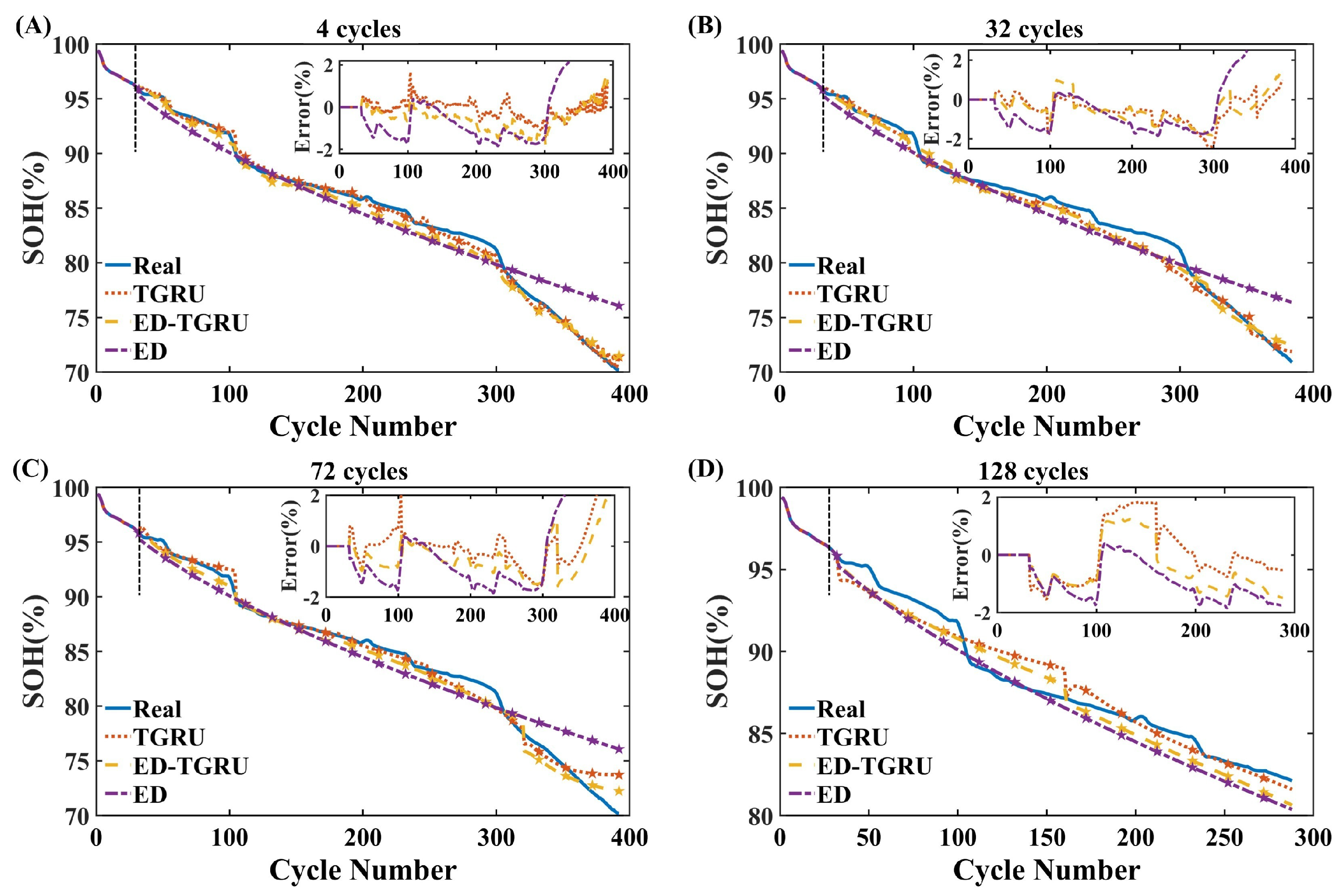
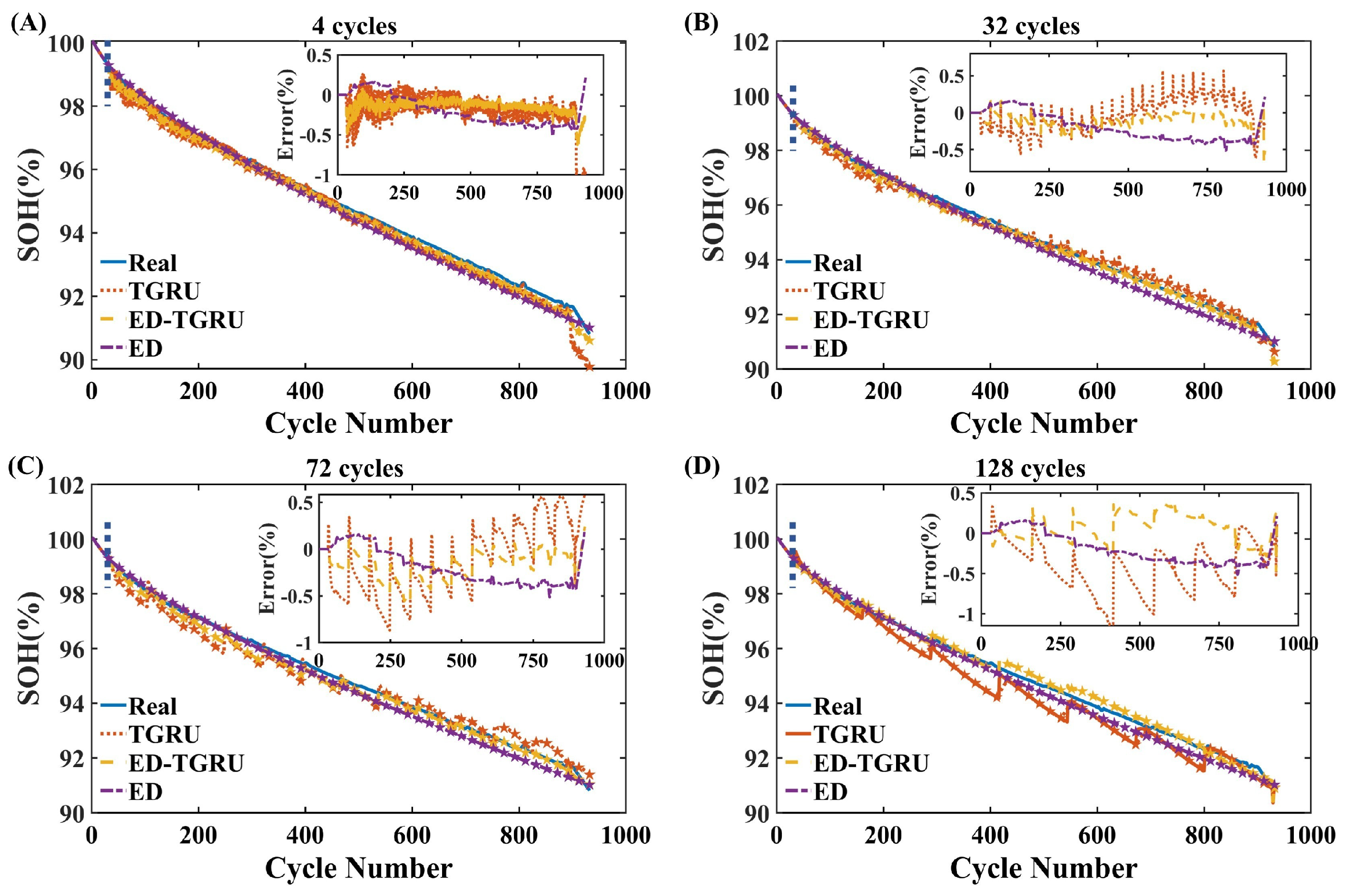
Due to pronounced cell-to-cell variability in manufacturing, initial health condition, and early-stage degradation behavior, we incorporated the first 30% of cycles from each test battery into the training process for joint training, enabling the model to adapt to the battery-specific initial degradation characteristics in the test set. Model performance was evaluated exclusively on the remaining 70% of cycles. To validate the effectiveness of the proposed method, comparisons were made using an empirical degradation model, a Transformer–GRU model, and the proposed empirical degradation-guided Transformer–GRU model. The SOH prediction results and their error distributions for cells B7, B10, and B12 at different time scales are shown in Figure 8, Figure 9, Figure 10 and Figure 11.
Figure 8.
Comparison of prediction performance for the different prediction cycles of B4. (A) for the next 4 cycles, (B) for the next 32 cycles, (C) for the next 72 cycles, (D) for the next 128 cycles.
Figure 9.
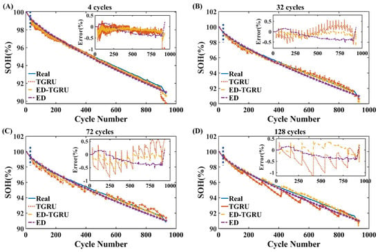
Comparison of prediction performance for the different prediction cycles of B7. (A) for the next 4 cycles, (B) for the next 32 cycles, (C) for the next 72 cycles, (D) for the next 128 cycles.
Figure 10.
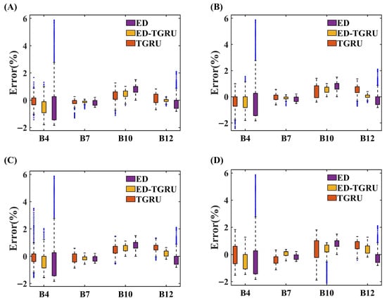
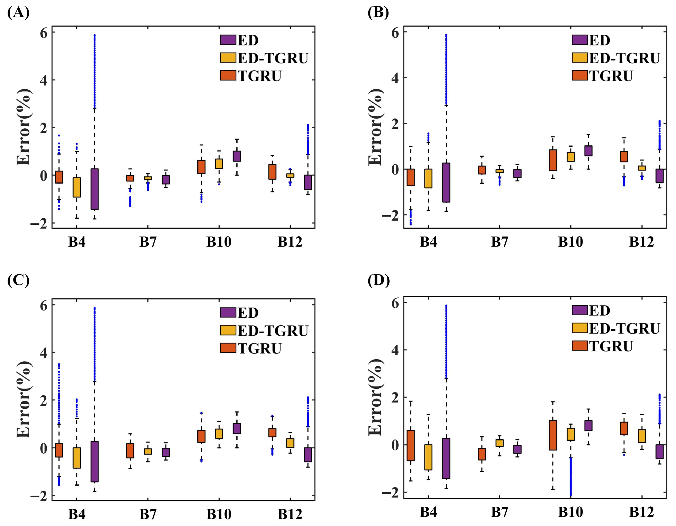
Comparison of box plots of prediction error of different models for the different prediction cycles. (A) for the next 4 cycles, (B) for the next 32 cycles, (C) for the next 72 cycles, (D) for the next 128 cycles.
Figure 11.
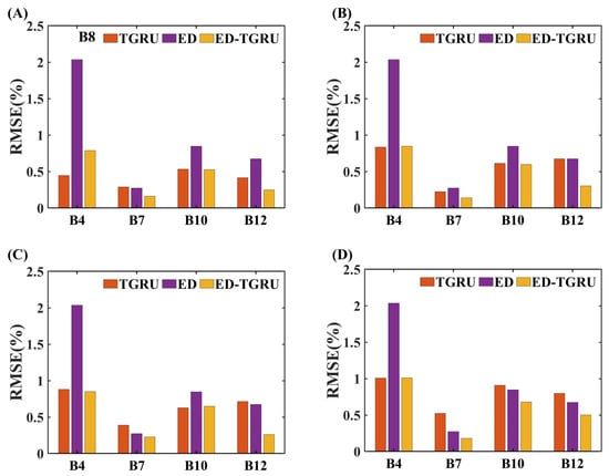
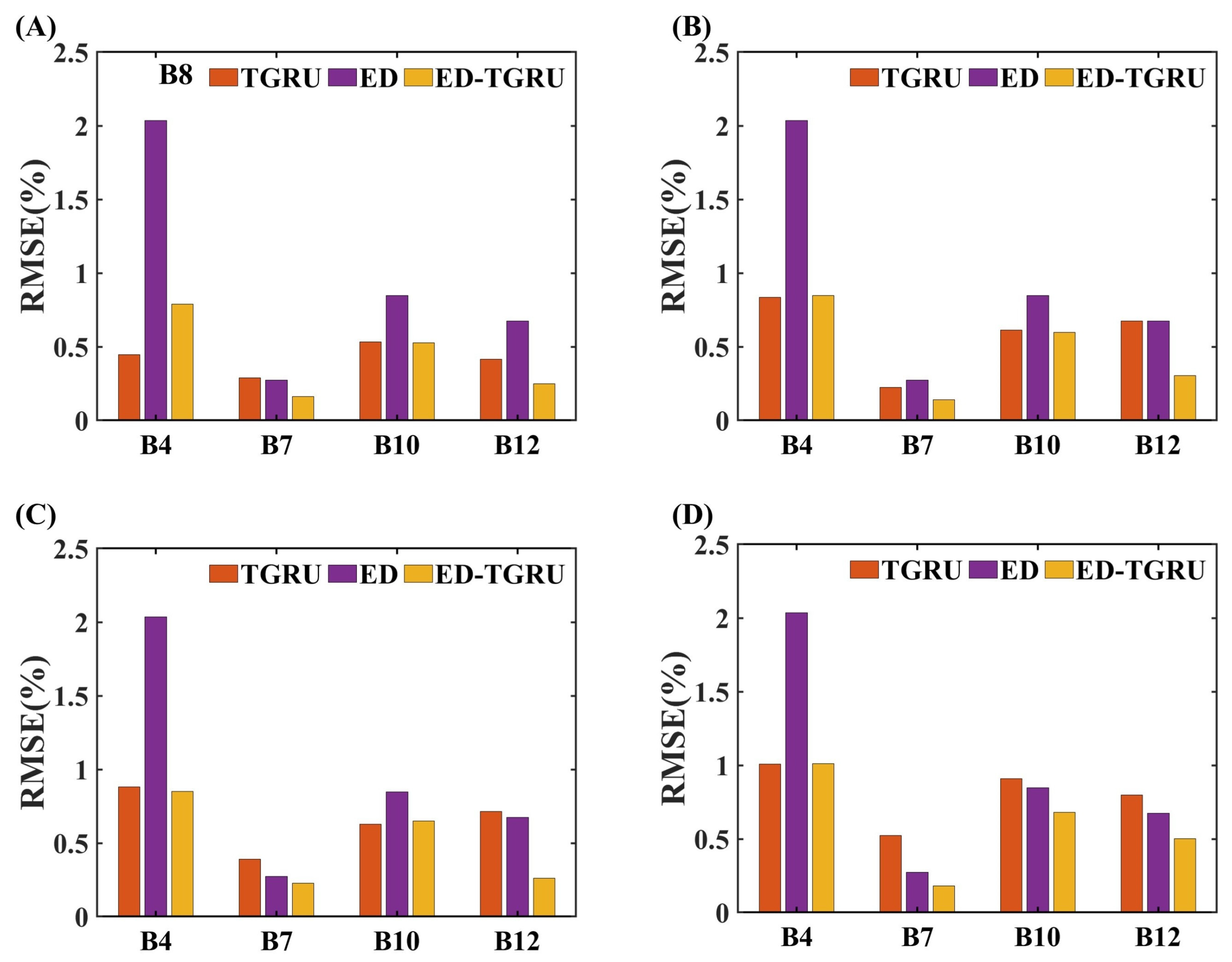
RMSE from model comparison experiments on different batteries for the different prediction cycles. (A) for the next 4 cycles, (B) for the next 32 cycles, (C) for the next 72 cycles, (D) for the next 128 cycles.
Figure 8 demonstrates the prediction performance of various models across different prediction cycles for cell B4. All three models exhibited strong performance in predicting the SOH for the first 300 cycles. However, after 300 cycles, cell B4 experienced a capacity “plunge” phenomenon. Following this plunge, the SOH predictions from the ED model began to deviate from the true values, whereas both the ED-TGRU and TGRU models continued to accurately track the battery capacity degradation trajectory. It is noteworthy that, for cell B4, the TGRU model outperformed the ED-TGRU model in SOH prediction regardless of the time scale. As observed from the prediction error box plots of each model in Figure 10, the TGRU model demonstrated superior performance over the ED-TGRU model in terms of the concentration of prediction errors, the number of outliers, and the deviation of outliers from the true values. Under various experimental conditions, the RMSE of the ED-TGRU model’s predictions ranged from a maximum of 1.01% to a minimum of 0.79%, with an average value of 0.87%. In comparison, the RMSE of the TGRU model’s predictions ranged from a maximum of 1.00% to a minimum of 0.44%, with an average value of 0.79%.
Therefore, in predicting the capacity degradation trajectory under low-temperature conditions, the TGRU model demonstrated the best prediction performance regardless of the forecast horizon, followed by the ED-TGRU model, while the ED model consistently performed the worst. This is because the empirical model developed in this study is only applicable within the normal range of battery capacity degradation. Although the parameters in the ED model account for the influence of test environment temperature, it fails to capture lithium plating—a phenomenon highly prone to occur during battery operation in low-temperature environments. The lithium plating-induced accelerated loss of lithium inventory and negative electrode active material capacity cannot be represented in the ED model. When predicting the SOH of batteries under low-temperature conditions, the ED-TGRU model is negatively influenced by the ED component, which reduces its prediction performance. In contrast, the TGRU model is free from interference by the ED component. Its input capacity sequence features and incremental capacity (IC) curve features contain information about the accelerated capacity degradation caused by lithium plating, enabling the model to align more closely with the true values during training. Therefore, the TGRU model is highly recommended as the preferred choice for predicting the capacity degradation trajectory of batteries operating under low-temperature conditions.
Furthermore, in the comparative experiments on prediction time horizons, it was observed that, as the number of prediction cycles increases, the performance of the TGRU model gradually deteriorated. This is reflected in a decreased concentration of prediction errors, an increased number of outliers, and a greater deviation of outliers from the true values. Specifically, the RMSE was 0.44% when predicting the next 4 cycles, but rose to 1.01% when predicting the next 128 cycles. We hypothesize that this is related to error accumulation and the inherent limitations of the model. The model employs a rolling window approach for data input, and as the prediction time horizon lengthens, the cumulative effect of errors becomes more pronounced. On the other hand, this phenomenon may also be influenced by the model’s inductive bias and the limitations of the training data. Therefore, when predicting the capacity degradation trajectory of batteries operating under low-temperature conditions, it is recommended to prioritize the TGRU model and adopt a short-term prediction approach, forecasting the degradation trajectory for the next 10 or 20 cycles. Particularly in addressing the accelerated capacity decay caused by lithium plating under low temperatures, selecting an appropriate prediction time scale holds significant potential for accurately predicting the “capacity plunge” point and the subsequent degradation trend after this plunge.
Figure 9 illustrates the prediction performance of various models across different cycle numbers for cell B7. As can be seen from Table 3 and Table 4, the RMSE of the ED-TGRU model was consistently less than 50% of that of the TGRU model for battery B7 across all prediction time scales. From the error curves and box plots in Figure 10, both the ED-TGRU and TGRU models showed almost no outliers, but the error concentration of the ED-TGRU model was significantly better than that of the TGRU model. Under various experimental conditions, the RMSE of the ED-TGRU model’s predictions ranged from a maximum of 0.23% to a minimum of 0.14%, with an average of 0.18%. In comparison, the RMSE of the TGRU model’s predictions ranged from a maximum of 0.52% to a minimum of 0.22%, with an average of 0.36%. Therefore, when predicting the capacity degradation trajectory under 25 °C conditions, the ED-TGRU model demonstrated the best prediction performance regardless of the forecast horizon, followed by the TGRU model, while the ED model consistently performed the worst.
Table 3.
RMSE from model comparison experiments on different batteries.
Table 4.
MAE from model comparison experiments on different batteries.
Data analysis from previous sections indicates that the ED model can also demonstrate satisfactory performance in predicting the SOH of batteries operating at room temperature. However, with the gradual increase in the capacity of lithium-ion cells in the energy storage field—taking the 314 Ah LFP cell as an example—a 1% SOH error corresponds to a capacity deviation of 3.14 Ah and an energy deviation of 10.048 Wh. Taking a battery cluster comprising eight battery packs as an example, where each pack contains eight modules and each module consists of 16 cells, the total number of cells in the cluster is 1024, corresponding to an energy error of 10.3 kWh. Even when applying the TGRU model, with its average error of 0.36%, the resulting capacity error per cell is 1.13 Ah, translating to an energy error of 3.7 kWh for the entire cluster. In comparison, the ED-TGRU model yields a cell capacity error of 0.56 Ah, corresponding to an energy error of 1.85 kWh. When evaluating battery SOH prediction requirements from the perspective of capacity or energy accuracy, it becomes evident that higher-precision models are necessary for accurate SOH prediction. Consequently, the superiority of the ED-TGRU model is fully demonstrated when considering the implications for battery capacity or energy estimation errors.
The ED model effectively incorporates the Arrhenius equation in its formulation for predicting the state of health (SOH) of batteries operating under room or elevated temperatures. This allows it to accurately describe the influence of temperature on the rate of battery capacity degradation. In contrast, due to inherent limitations in its parameter learning, the TGRU model may fail to adequately capture the underlying patterns of capacity fade under certain specific conditions. By integrating the ED model, constraints can be applied to the TGRU model when its predictions begin to deviate from the true values, thereby keeping the forecast results oscillating within an acceptable range near the actual measurements, as illustrated in Figure 9C,D. In long-term predictions—specifically when forecasting SOH for 72 and 128 cycles ahead—the TGRU model showed significant deviation in the predicted trajectory. In comparison, the ED-TGRU model, benefiting from the constraints imposed by the ED component, effectively mitigated this issue and delivered superior prediction performance.
Figure 10 depicts the error metric plots for SOH predictions across all test-set batteries at different time scales. It can be observed that the constraining effect of the ED model on the TGRU model also held true for cells B10 and B12. Across all experimental setups, the ED-TGRU model consistently achieved lower RMSE values than the TGRU model, demonstrating that the proposed ED-TGRU model exhibits excellent performance under room or elevated temperature conditions. The RMSE of the ED-TGRU model’s SOH predictions for cells B7, B10, and B12 under three temperature conditions ranged from a maximum of 0.68% to a minimum of 0.14%, with an average of 0.37%. Taking the aforementioned battery cluster as an example, the maximum cell capacity error is 2.13 Ah and the minimum is 0.44 Ah, corresponding to a maximum cluster energy error of 7 kWh and a minimum of 1.44 kWh. Therefore, improving the accuracy of battery SOH prediction can provide crucial support for full life-cycle management and energy management of battery systems.
5. Conclusions
This paper proposes a Transformer–GRU model integrated with empirical degradation trends, primarily accomplishing the following work:
(1) A dataset of lithium-ion battery capacity degradation under wide-temperature-range and multi-operating-condition scenarios was constructed, and capacity-related features highly correlated with battery capacity fade were extracted from the raw data.
(2) An empirical degradation-guided Transformer–GRU model (abbreviated as ED-TGRU) was proposed for predicting the battery state of health degradation trajectory. The model integrates prior knowledge of empirical degradation trends with deep sequence modeling capabilities. It is mainly composed of four components: a self-attention encoder (Transformer Encoder), a recurrent decoder (GRU Decoder), an empirical degradation prior module (Empirical Degradation Prior Module), and an adaptive fusion gate (Adaptive Fusion Gate), designed to support short-term, medium-term, and long-term SOH degradation prediction tasks.
(3) The proposed method can accurately predict the capacity degradation trends of batteries under different degradation mechanisms. The ED-TGRU model demonstrates excellent SOH prediction performance, achieving an average RMSE of 0.87% with a minimum of 0.79% in low-temperature environments, while under room or elevated temperatures, its RMSE ranges from a maximum of 0.68% to a minimum of 0.14%, with an average of 0.37%.
Author Contributions
Conceptualization, X.L., C.L. and Z.C.; Methodology, X.L., J.F. and C.Z.; Software, C.L.; Validation, X.L. and C.L.; Formal analysis, C.L. and S.G.; Investigation, X.L., C.L. and Z.C.; Resources, X.L., C.L. and Z.C.; Data curation, X.L. and Z.C.; Writing—original draft preparation, X.L., C.L. and Z.C.; Writing—review and editing, Z.C., J.F. and C.Z.; Visualization, X.L. and S.G.; Supervision, J.F., S.G. and C.Z.; Project administration, Z.C. and J.F.; Funding acquisition, C.Z. All authors have read and agreed to the published version of the manuscript.
Funding
This research study was funded by the Young Scientists Fund of the National Natural Science Foundation of China (Grant No. 52222708) and the Fundamental Research Funds for the Central Universities (Science and technology leading talent team project) (Grant No. 2022JBQY008).
Data Availability Statement
The data presented in this study are available on request from the corresponding author. The data are not publicly available due to confidentiality of ongoing projects.
Conflicts of Interest
Author Xiandao Lei was employed by the company China Three Gorges Renewables Group Co., Ltd. The remaining authors declare that the research was conducted in the absence of any commercial or financial relationships that could be construed as a potential conflict of interest.
Abbreviations
The following abbreviations are used in this manuscript:
| V-Q | Voltage-capacity |
| SOH | State of health |
| ED | Empirical degradation |
| GRU | Gated recurrent unit |
| TGRU | Transformer–GRU |
| ED-TGRU | Empirical degradation-guided Transformer–GRU |
| SEI | Solid electrolyte interphase |
| ECMs | Equivalent circuit models |
| EMs | Electrochemical models |
| GPR | Gaussian process regression |
| IC | Incremental capacity |
| DV | Differential voltage |
| LFP | Lithium iron phosphate |
| CC | Constant current charging |
| DC | Constant current discharging |
| MCC | Multi-stage constant current charging |
| DCR | Direct current internal resistance |
| NLP | Natural language processing |
| RUL | Remaining useful life |
| MSE | Mean squared error |
| MAE | Mean absolute error |
| RMSE | Root mean squared error |
Appendix A
Figure A1 provides the current and voltage of charging protocol for 1.6 C (MCC) and 1 C (MCC). 1.6 C or 1 C refer to the average rate from 20% SOC to 80% SOC.
Figure A1.
The current and voltage of charging protocol for 1.6 C MCC and 1 C MCC.
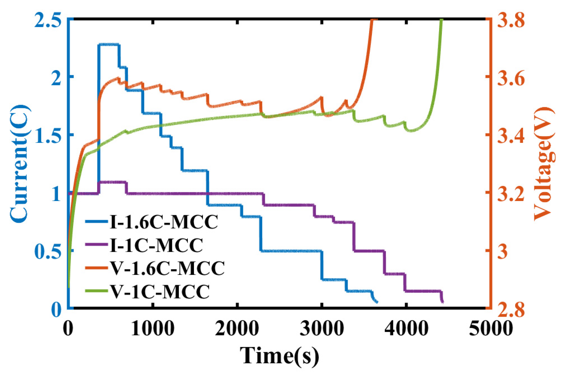
Table A1.
The test schedule of cycle test and capacity test.
References
- Sbarufatti, C.; Corbetta, M.; Giglio, M.; Cadini, F. Adaptive prognosis of lithium-ion batteries based on the combination of particle filter sand radial basis function neural networks. J. Power Sources 2017, 344, 128–140. [Google Scholar] [CrossRef] [Scilit]
- An, S.J.; Li, J.; Daniel, C.; Mohanty, D.; Nagpure, S.; Wood, D.L. The state of understanding of the lithium-ion-battery graphite solid electrolyte interphase (SEI) and its relationship to formation cycling. Carbon 2016, 105, 52–76. [Google Scholar] [CrossRef] [Scilit]
- Yang, L.; Takahashi, M.; Wang, B. A study on capacity fading of lithium-ion battery with manganese spinel positive electrode during cycling. Electrochim. Acta 2006, 51, 3228–3234. [Google Scholar] [CrossRef] [Scilit]
- Merrouche, W.; Lekouaghet, B.; Bouguenna, E.; Himeur, Y. Parameter estimation of ECM model for Li-ion battery using the weighted mean of vectors algorithm. J. Energy Storage 2024, 76, 109891. [Google Scholar] [CrossRef] [Scilit]
- Liu, Z.; Zhao, Z.; Qiu, Y.; Jing, B.; Yang, C. State of charge estimation for Li-ion batteries based on iterative Kalman filter with adaptive maximum correntropy criterion. Power Sources 2023, 580, 233282. [Google Scholar] [CrossRef] [Scilit]
- Amir, S.; Gulzar, M.; Tarar, M.O.; Naqvi, I.H.; Zaffar, N.A.; Pecht, M.G. Dynamic equivalent circuit model to estimate state-of-health of lithium-ion batteries. IEEE Access 2022, 10, 18279–18288. [Google Scholar] [CrossRef] [Scilit]
- Yu, H.; Zhang, L.; Wang, W.; Li, S.; Chen, S.; Yang, S.; Li, J.; Liu, X. State of charge estimation method by using a simplified electrochemical model in deep learning framework for lithium-ion batteries. Energy 2023, 278, 127846. [Google Scholar] [CrossRef] [Scilit]
- Liu, Y.; Wang, L.; Li, D.; Wang, K. State-of-health estimation of lithium-ion batteries based on electrochemical impedance spectroscopy: A review. Prot. Control Mod. Power Syst. 2023, 8, 41. [Google Scholar] [CrossRef] [Scilit]
- Xiong, R.; Li, L.; Tian, J. Towards a smarter battery management system: Acritical review on battery state of health monitoring methods. J. Power Sources 2018, 405, 18–29. [Google Scholar] [CrossRef] [Scilit]
- Zhang, Y.; Xiong, R.; He, H.; Petch, M.G. Lithium-ion battery remaining useful life prediction with box-cox transformation and Monte Carlo simulation. IEEE Trans. Ind. Electron. 2019, 66, 1585–1597. [Google Scholar] [CrossRef] [Scilit]
- Severson, K.A.; Attia, P.M.; Jin, N.; Perkins, N.; Jiang, B.; Yang, Z.; Chen, M.H.; Aykol, M.; Herring, P.K.; Fraggedakis, D.; et al. Data-driven prediction of battery cycle life before capacity degradation. Nat. Energy 2019, 4, 383–391. [Google Scholar] [CrossRef] [Scilit]
- Richardson, R.R.; Birkl, C.R.; Osborne, M.A.; Howey, D.A. Gaussian process regression for in situ capacity estimation of Lithium-ion batteries. IEEE Trans. Ind. Inform. 2019, 15, 127–138. [Google Scholar] [CrossRef] [Scilit]
- He, J.; Bian, X.; Liu, L.; Wei, Z.; Yan, F. Comparative study of curve determination methods for incremental capacity analysis and state of health estimation of lithium-ion battery. J. Energy Storage 2020, 29, 101400. [Google Scholar] [CrossRef] [Scilit]
- Tagade, P.; Hariharan, K.S.; Ramachandran, S.; Khandelwal, A.; Naha, A.; Kolake, S.M.; Han, S.H. Deep Gaussian process regression for lithium-ion battery health prognosis and degradation mode diagnosis. J. Power Sources 2020, 445, 227281. [Google Scholar] [CrossRef] [Scilit]
- Yang, X.; Xie, H.; Zhang, L.; Yang, K.; Liu, Y.; Chen, G.; Ma, B.; Liu, X.; Chen, S. Early-stage degradation trajectory prediction for lithium-ion batteries: A generalized method across diverse operational conditions. J. Power Sources 2024, 612, 234808. [Google Scholar] [CrossRef] [Scilit]
- Li, W.; Sengupta, N.; Dechent, P.; Howey, D.; Annaswamy, A.; Sauer, D.U. One-shot battery degradation trajectory prediction with deep learning. J. Power Sources 2021, 506, 230024. [Google Scholar] [CrossRef] [Scilit]
- Sun, J.; Lou, J.; Kainz, J. A degradation trajectory prediction method applicable to various life stages of lithium-ion batteries under complex variable aging conditions. Appl. Energy 2025, 398, 126425. [Google Scholar] [CrossRef] [Scilit]
- Li, F.; Feng, H.; Min, Y.; Zhang, Y.; Zuo, H.; Bai, F.; Zhang, Y. Prediction of lithium-ion battery degradation trajectory in electric vehicles under real-world scenarios. Energy 2025, 317, 134663. [Google Scholar] [CrossRef] [Scilit]
- Zhou, J.; Rong, J.; Zhang, J.; Liu, C.; Yi, F.; Jiao, Z.; Zhang, C. Deep learning estimation of state of health for lithium-ion batteries using multi-level fusion features of discharge curves. J. Power Sources 2025, 653, 237781. [Google Scholar] [CrossRef] [Scilit]
- Tian, J.; Xiong, R.; Shen, W.; Lu, J.; Yang, X.-G. Deep neural network battery charging curve prediction using 30 points collected in 10 min. Joule 2021, 5, 1521–1534. [Google Scholar] [CrossRef] [Scilit]
- Wang, J. State of Health Estimation and Degradation Prediction of Power Batteries Considering the Operation Characteristics of Electric Vehicles; Beijing Jiaotong University: Beijing, China, 2024. [Google Scholar]
- Guo, Q.; Zhang, C.; Gao, Y. Incremental Capacity Curve Based State of Health Estimation for LNMCO Lithium-ion Batteries. J. Glob. Energy Interconnect. 2018, 1, 180–187. (In Chinese) [Google Scholar]
- Barré, A.; Deguilhem, B.; Grolleau, S.; Gérard, M.; Suard, F.; Riu, D. A review on lithiumion battery ageing mechanisms and estimations for automotive applications. J. Power Sources 2013, 241, 680–769. [Google Scholar] [CrossRef] [Scilit]
- Vaswani, A.; Shazeer, N.; Parmar, N.; Uszkoreit, J.; Jones, L.; Gomez, A.N.; Kaiser, L.; Polosukhin, I. Attention is all you need. Adv. Neural Inf. Process. Syst. 2017, 30. [Google Scholar] [CrossRef] [Scilit]
- Hou, G.; Zhang, F.; Huang, C.; Huang, T. Joint prediction of SOH and RUL for Lithium-ion batteries by an enhanced Transformer model with physical information constraints. Energy 2025, 336, 138435. [Google Scholar] [CrossRef] [Scilit]
- Ding, G.; Wang, W.; Zhu, T. Remaining Useful Life Prediction for Lithium-Ion Batteries Based on CS-VMD and GRU. IEEE Access 2022, 10, 89402–89413. [Google Scholar] [CrossRef] [Scilit]

Disclaimer/Publisher’s Note: The statements, opinions and data contained in all publications are solely those of the individual author(s) and contributor(s) and not of MDPI and/or the editor(s). MDPI and/or the editor(s) disclaim responsibility for any injury to people or property resulting from any ideas, methods, instructions or products referred to in the content. |
© 2026 by the authors. Licensee MDPI, Basel, Switzerland. This article is an open access article distributed under the terms and conditions of the Creative Commons Attribution (CC BY) license.