


Abstract
Camellia japonica is a widely cultivated woody ornamental plant. However, current studies mostly focus on the onset of flowering, neglecting the overall flowering time distribution patterns of the blooming process. In this study, we used uniform 5-year-old potted cuttings of C. japonica ‘Jinjiang Mudan’ to evaluate six candidate distribution models, including normal, log-normal, skew-normal, gamma, Weibull, and exponential, to model flowering time distribution. These candidates were compared to obtain an optimal distribution model using three-fold cross-validation, six evaluation indicators, and three goodness-of-fit tests in the control. The optimal distribution model was used to compare and analyze the different effects of the control, shading, and exogenous hormone treatments. The results showed that the skew-normal distribution model emerged as the most suitable distribution model among the six candidates and captured the flowering time distribution characteristics effectively in all treatments. Shading treatments were found to delay and extend the flowering period, with moderate treatments (50% and 70% shading) demonstrating better performance, extending the flowering period by approximately 40%. In terms of exogenous hormone treatments, BG (a mixture of the 6-BA and GA3) concentrations could prolong and delay the flowering period. Lower concentrations (100 and 250 mg L−1) of 6-BA and GA3 were effective in extending the flowering period, with BA250 exhibiting the most pronounced effect, delaying flowering onset by approximately 12% and extending the flowering period by approximately 17%. Considering that this study is based on single-location and single-season trials, these findings provide a valuable methodological resource for quantifying and predicting flowering time distribution in C. japonica, other ornamentals, and crops.
1. Introduction
Camellia japonica is a globally significant ornamental plant, boasting thousands of cultivars that exhibit diverse floral variations [1]. Unlike many other ornamental horticultural crops, C. japonica blooms primarily in winter, a time when very few flowers are available in commercial markets [2,3]. Furthermore, the compact growth habit of C. japonica makes it particularly suitable for pot culture, reinforcing its popularity as a major potted ornamental [4,5]. How to maximize this economic potential by precisely scheduling flowering to align with peak consumer demand, like during the Spring Festival in China, is an important research direction.
In practice, hormonal treatments (e.g., gibberellins, paclobutrazol) and photoperiodic regulation are widely used to change flowering time to meet market demands [1,3,5]. For commercial producers, the profitability of C. japonica, whether as potted plants or cut flowers, depends largely on predictable flowering schedules that align with market demand. However, current studies primarily focus on the timing of the first flowering, which provides limited guidance for large-scale production [4,6,7]. The ability to predict and control the full temporal distribution of flowering is therefore of considerable commercial importance. Reliable models would enable growers to forecast peak bloom periods and overall yield more accurately, allowing better optimization of greenhouse space, more efficient labor allocation for harvesting and packaging, and reduced post-harvest losses from asynchronous flowering. For producers in particular, synchronized bloom timing ensures uniform flower maturity within bunches, consistent quality for wholesale buyers, and better alignment with shipping and market windows [8]. Moreover, establishing a solid quantitative baseline of flowering dynamics is critical for objectively evaluating the effectiveness of common commercial practices such as shading and exogenous hormone applications.
Unfortunately, a robust quantitative framework for flowering dynamics remains lacking. Flowering phenology is rarely symmetrical; it is typically asymmetrical and has a skewed distribution, characterized by distinct onset, peak, and termination phases [9]. Traditional descriptive statistics and models, which assume a normal distribution, may miss important temporal features like skewness and tail extension [10]. The lack of a robust quantitative framework hinders accurate prediction and regulation of the flowering period.
Motivated by the need to bridge this gap between descriptive observation and mathematically grounded prediction in horticultural practice, the present study employed the potted C. japonica cultivar ‘Jinjiang Mudan’ to develop a quantitative model of flowering phenology. Specifically, our goals were as follows: (1) identify the best distribution model for bloom dynamics; (2) analyze the effects of shading and hormones on flowering time distribution; and (3) understand the key regulatory roles of shading and hormones. By shifting from simple onset dates to a comprehensive distribution-based analysis, this work offers new theoretical insights and practical tools for the precise flowering prediction of C. japonica.
2. Materials and Methods
2.1. Plant Material and Experimental Site
Uniform 5-year-old potted cuttings of C. japonica ‘Jinjiang Mudan’ were tested in this study. Before the experiment, all plants were cultivated together on 1 January 2025, at the Hengxi Research Station of Ningbo Academy of Agricultural Sciences in Ningbo City, Zhejiang Province, China (121°35′ E, 29°40′ N), under natural photoperiod and full sunlight conditions to ensure growth uniformity. The site where the experiment was performed has a subtropical monsoon climate, with a mean annual temperature of 16.7 °C and a mean annual precipitation of 1400–1500 mm [11]. The plants selected had consistent morphological traits. Exogenous hormones, including 6-benzylaminopurine (6-BA) and Gibberellic acid (GA3), were both obtained from Coolaber Science & Technology (Beijing, China).
2.2. Experimental Design
The study was conducted on 20 January 2025 (bud stage) and consisted of two parallel, independent trials. For the shading experiment, four treatments were established using black polyethylene shade nets to provide 30% (S30), 50% (S50), 70% (S70), and 90% (S90) shading rates. To ensure true statistical replication and avoid spatial confounding effects, three independent shade nets were constructed for each shading treatment. These independent shade nets were randomly distributed across the experimental site. Each individual shade net contained 5 potted plants. Notably, shade structures were constructed with sufficient height (1.6 m) with open sides to guarantee ventilation, thereby minimizing temperature differentials between treatments and the control.
Exogenous hormone treatments were conducted under natural light conditions using 6-BA and GA3, at 100, 250, 500, and 1000 mg L−1, or a mixture of the two equal volumes [12]. To avoid phytotoxicity due to extreme pH, we used absolute ethanol (C2H6O, ≥99.7%) as the initial solvent instead of strong acids or bases. For the 6-BA treatments, the required amount of pure powder was first dissolved in 10 mL of absolute ethanol per liter of final volume, then diluted with distilled water [13,14]. Because of the low water solubility of 6-BA, the final preparation formed a suspension (pH 7.6) rather than a clear solution. In contrast, GA3 prepared using the same protocol produced a clear solution (pH 3.4). The combined BG treatments also resulted in suspensions. The hormonal treatments were applied as foliar sprays only. During application, sprayers containing the suspensions were gently and continuously agitated to ensure uniform delivery of the active ingredient. Each plant was sprayed twice using a standard procedure: the entire canopy was first sprayed until runoff, and a second spray was applied as soon as the leaves had dried to promote maximum absorption [1,5]. All treatments were conducted with 3 independent replicates, with 5 plants per replicate.
A separate group of plants, designated as the control treatment (CK), was maintained alongside the hormone-treated plants under identical natural light conditions. They received neither shading nor hormone application (Table 1).
Table 1.
Hormone treatments with different concentrations.
2.3. Data Collection and Reconstruction
2.3.1. Data Collection
The daily flowering counts were recorded starting from the date when the absolute first open flower was observed across all experimental units, which coincided with the simultaneous onset of flowering in the BA100, BA500, and BA1000 treatment groups. This initial blooming event occurred on 25 February 2025, designated as day of year (DOY) 56. The net number of flowers (NNF) was defined as the cumulative number of flowers minus the number of fallen flowers. The NNF per plant was recorded at 2- to 3-day intervals until the last flower withered. The last flower withered on 29 June 2025, that is 180 DOY. Thus, DOY and NNF datasets were obtained.
2.3.2. Data Reconstruction
In order to better describe the flowering time distribution, the total NNF (TNF) of 5 plants per replicate was used as the treatment-level value. The DOY and TNF datasets were reconstructed using the rep function in R, replicating each DOY by its corresponding TNF, as shown in Table 2.
Table 2.
Summary statistics for reconstructed data (mean ± standard deviation).
Three-fold cross-validation was employed to evaluate model generalizability, prevent overfitting, and ensure equitable validation [15,16,17,18,19,20]. In each fold, two replicates of reconstructed data were used as the training data, and the rest were used as the test data.
2.4. Model Evaluation
2.4.1. Candidate Distribution Models
Six commonly distributed models were used as candidates: normal, log-normal, skew-normal, gamma, Weibull, and exponential distribution models. The random variable X follows a distribution. In this study, both the training and test data were treated as a random variable X. Their specific probability density functions (PDFs) are as follows [21,22,23,24]:
where f(x) is the PDF, F(x) is the cumulative distribution function (CDF), and Q(p) is the quantile distribution function (QDF). Equation (1) is normal, Equation (2) is log-normal, Equation (3) is skew-normal, Equation (4) is gamma, Equation (5) is Weibull, and Equation (6) is exponential. Equation (7) is the CDF of f(x), Equation (8) is the QDF of f(x), and p is the probability. QDF is the inverse function of CDF. Equation (9) is the PDF of the standard normal, and Equation (10) is the CDF of the standard normal. Μ and σ are the mean and standard deviation (SD) of x in Equation (1). μ and σ are the mean and SD of lnx in Equation (2). ξ, ω, and α are the location, scale, and shape parameters. In Equation (3), α = 0 recovers normal, α > 0 gives right skew, and α < 0 gives left skew. x is a specific value of the random variable X, and f(x) is the probability density of x.
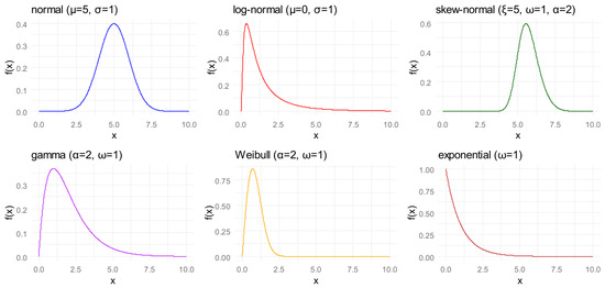
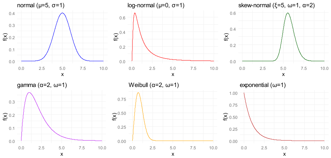
In this study, x denotes a specific DOY of reconstructed data, and f(x) denotes the probability density of TNF at a specific DOY. These equations were constructed with the “fitdistrplus” and “sn” packages in R version 4.5.2 [22,25]. For instance, when μ = 5 and σ = 1 in Equation (1); μ = 0 and σ = 1 in Equation (2); and ξ = 5, ω = 1, and α = 2, the horizontal axis ranges from 0 to 10. These six PDF graphs are shown in Figure 1.
Figure 1.
Six PDFs of distribution model.
The normal distribution model is frequently used for phenological events approximating Gaussian behavior [26]. The log-normal and gamma distribution models allow right skewing to accommodate delayed early flowering, which is common in many horticultural crops [19]. The Weibull distribution model effectively captures the variable rate of flowering progression in fruit trees and perennials, as its universal shape parameter allows it to capture both increasing and decreasing risk functions [15]. The skewed normal distribution model addresses the deficiency of standard normal fitting for a slightly skewed dataset due to its three parameters [23].
2.4.2. Evaluation Criteria
Six model evaluation indicators were selected to identify the best-fitting distribution model, including Akaike Information Criterion (AIC), Bayesian Information Criterion (BIC), log-likelihood (LogLik), mean absolute error (MAE), maximum absolute error (MaxAE), and root mean square error (RMSE). Their formulas are as follows [27,28,29]:
where is the LogLik value and is the optimal parameter vector obtained by maximum likelihood estimation. k is the dimension of , as well as the number of estimated parameters. xi is the i-th specific value of the random variable X, is the probability density of xi evaluated at , and n is the sample size. is the j-th probability value. is the quantile of the sample data at a given , is the predicted QDF value at given , and m is the number of given .
Quantiles were selected to describe the distribution characteristics of the flowering period, with quantiles corresponding to the following developmental stages [30]: the 5th percentile (Q5) denotes initial flowering time, the 25th percentile (Q25) denotes onset of peak bloom time, the 75th percentile (Q75) denotes end of peak bloom time, and the 95th percentile (Q95) denotes terminal flowering time. Therefore, in this study, p1 = 1%, p2 = 5%, p3 = 10%, p4 = 25%, p5 = 50%, p6 = 75%, p7 = 90%, p8 = 95%, p9 = 99%, and m = 9.
When ΔAIC exceeds 10, the lower value indicates a better fit against the alternative [15,20]. LogLik can evaluate the model’s generalization performance; a higher value (i.e., less negative or approaching zero) indicates improved model fit. MAE, MaxAE and RMSE could, respectively, represent the mean deviation, outlier sensitivity and overall accuracy, where smaller values signify better fit [16,20,31]. Kolmogorov–Smirnov (KS), Anderson–Darling (AD), and Cramér–von Mises (CM) were selected to examine the goodness-of-fit. AD was sensitive to tail behavior, which is critical in phenological data [19,25].
The AIC, BIC, MAE, MaxAE, and RMSE were computed using the training data, while LogLik was evaluated using the test data. Goodness-of-fit of KS, AD, and CM was computed using the training data.
2.5. Distribution Characteristics Analysis
CK data were used to select the optimal distribution model by comparing and analyzing the six candidates. The optimal distribution model was used to model flowering progression across all treatments, including shading treatments and exogenous hormone treatments.
Nine statistics were selected to capture the full flowering time distribution curve: mean flowering time (Mean), median flowering time (Median), mode flowering time (Mode), initial flowering time (Q5), onset of peak bloom time (Q25), end of peak bloom time (Q75), terminal flowering time (Q95), peak bloom duration (the length between Q75 and Q25), and full flowering duration (the length between Q95 and Q5) [30,32]. Mean quantifies the central tendency of the flowering time distribution, Median identifies the time by which 50% of the flowering process, and Mode corresponds to the most frequent flowering time or the maximum in the probability density of the flowering time distribution. For each treatment, the Mean and Mode were calculated using the following formulas [24]:
where F(x) is CDF and f(x) is PDF; see Equations (1)–(7) for details.
Additionally, the Median, Q5, Q25, Q75, and Q95 were calculated using Equations (8) and (17), where pj = 50%, 5%, 25%, 75%, and 95%, respectively.
2.6. Statistical Analysis
All statistical computations were carried out in R version 4.5.2 [16,33], including data reconstruction, 3-fold cross-validation, model evaluation, distribution characteristic analysis, and others. Meanwhile, the principal packages utilized comprised fitdistrplus for parameter estimation and integrated diagnostics [25], sn for skew-normal models [22], goftest for the AD and CM tests [34], and reshape2 for data reconstruction [35].
3. Results
3.1. Model Selection
Six candidate distribution models were compared and analyzed using three-fold cross-validation in CK, with mean evaluation metrics across three folds, as shown in Table 3 and Table 4.
Table 3.
Mean performance metrics across three folds in CK.
Table 4.
Mean goodness-of-fit measures across three folds in CK.
The skew-normal distribution model had the lowest mean AIC (3685.67) and BIC (3698.04), with ΔAIC values exceeding 50 units compared to the log-normal distribution model (3736.02) and 68 units relative to the gamma distribution model (3754.57). The normal, Weibull, and exponential distribution models trailed substantially; the latter had the poorest performance (AIC 5025.11). The mean MAE (1.72) of the skew-normal distribution model was half that of log-normal (3.88) and gamma (4.50). The exponential distribution model had the highest mean MAE (89.73). The mean RMSE sorted from small to large is as follows: skew-normal distribution model (2.49), log-normal distribution model (4.70), gamma distribution model (5.43), and exponential distribution model (115.60). Meanwhile, the skew-normal distribution model had the lowest mean MaxAE (6.27) among the other five distribution models. Mean LogLik of test data was the highest for the skew-normal distribution model (−924.80), better than the log-normal distribution model (−937.04), the gamma distribution model (−942.17), and the exponential distribution model (−1255.85).
Mean goodness-of-fit measures across three folds rejected all models at α = 0.05 (Table 4). This may be attributed to the high sensitivity provided by the large number of observations per replicate. However, the skew-normal distribution model was the best performing among these distribution models, with the least mean statistic and the largest p value (mean KS statistic 0.1014, p value 0.0014; AD statistic 3.4374, p value 0.0256; CM statistic 0.6699, p value 0.0259).
In summary, the skew-normal distribution model was the optimal distribution model among the other five candidates and was adopted to model flowering progression across all treatments, including shading treatments and exogenous hormone treatments.
3.2. Flowering Distribution Characteristics in CK
The skew-normal distribution model was used to model flowering time distribution in CK, with mean statistics between the fitted skew-normal and the sample, as shown in Table 5. There was a slight difference in the mean flowering date between the fitted (89.1 DOY) and the sample (88.6 DOY). The absolute difference in Mean, SD, Median, and Mode was 0.5 days, −0.6 days, 1.1 days, and 0.1 days, respectively. The absolute difference in Q5, Q25, Q75, and Q95, respectively, was −0.9 days, 0.9 days, 2.1 days, and −0.6 days, denoting that quantile differences were ≤2.1 days. Moreover, full flowering durations (Q95–Q5) of the fitted and the sample were 47.0 days and 46.7 days, respectively. The peak bloom durations (Q75–Q25) of the fitted and the sample were 19.9 days and 18.7 days, respectively. It shows that the difference between the fitted and the sample is small in the full flowering duration and the peak bloom duration.
Table 5.
Mean statistics between fitted skew-normal and sample across three folds in CK.
Though the mean skewness and kurtosis of the fitted (0.88 and 0.74) were lower than those of the sample (1.08 and 0.93), the distribution shape was adequately captured. In terms of parameter estimation (Table 6), location (ξ), scale (ω), and shape (α) were 70.4 ± 0.1 DOY, 23.8 ± 1.4 DOY, and 5.8 ± 0.8 DOY, respectively. It shows that the position of the distribution core was stable, since the standard deviation of ξ was 0.1 days. There was a modest variation in ω and α, due to the standard deviation of ω and α being both ≤ 1.4 days.
Table 6.
Skew-normal parameter estimates across three folds (mean ± standard deviation).
Collectively, the skew-normal distribution model can well describe the distribution characteristics of the flowering period in CK.
3.3. Treatment Effects on Flowering Distribution Characteristics
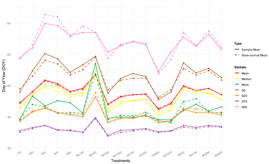
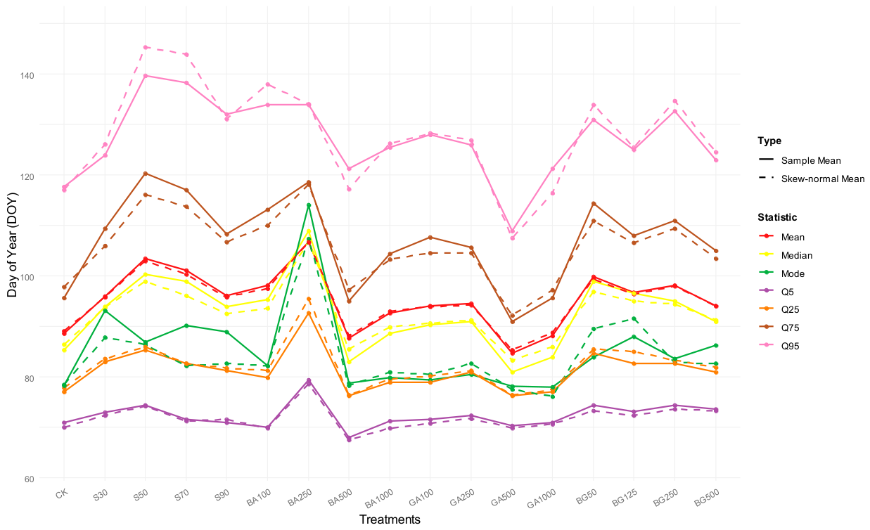
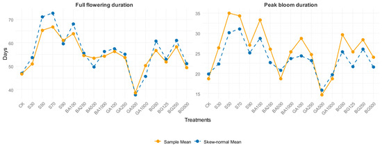
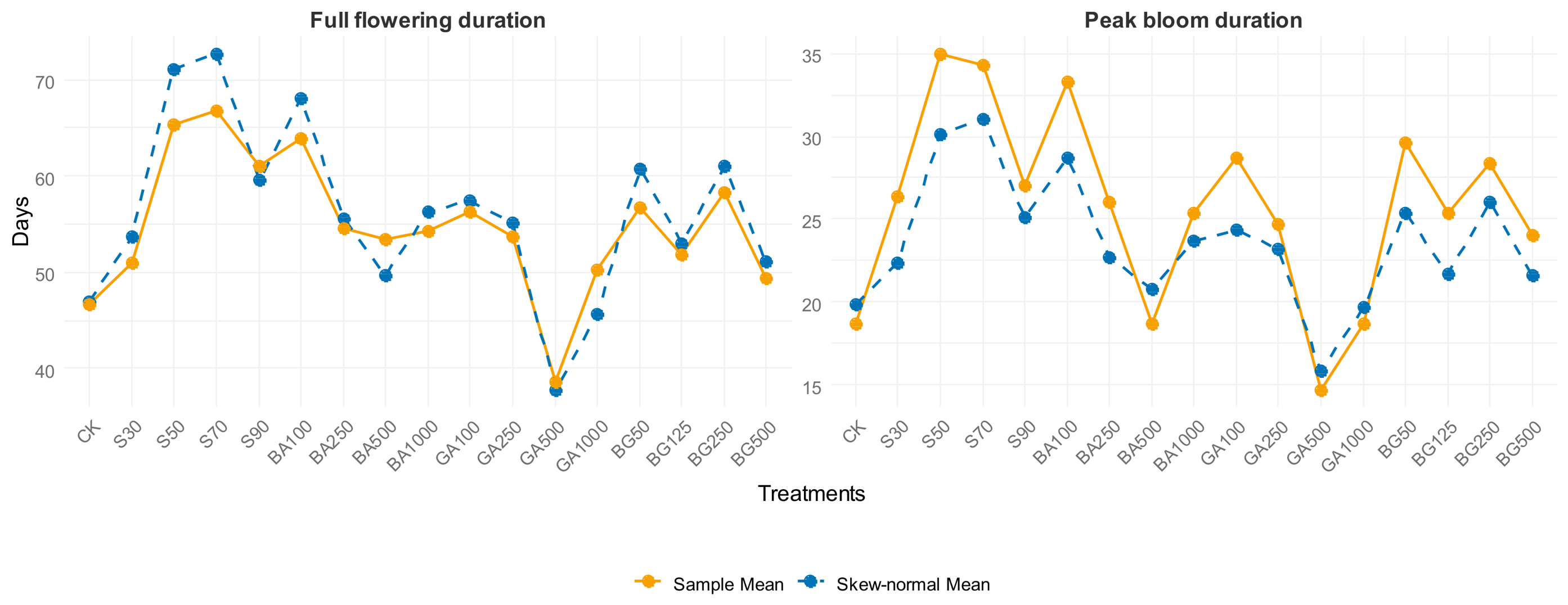
The skew-normal distribution model was employed to model flowering progression across all treatments, including shading treatments and exogenous hormone treatments. For each treatment, nine statistics, i.e., Mean, Mode, Median, Q5, Q25, Q75, Q95, peak bloom duration, and full flowering duration, were calculated using Equations (3), (7), (8) and (17)–(19) within the training data through three-fold cross-validation. Mean statistics across three folds between the fitted skew-normal and the sample, as shown in Figure 2 and Figure 3. Location (ξ), scale (ω), and shape (α) were estimated using three-fold cross-validation, as shown in Table 6.
Figure 2.
Distribution characteristics in different treatments. Solid lines denote mean statistics of sample across three folds, and dashed lines denote mean statistics of skew-normal across three folds.
Figure 3.
Flowering durations in different treatments. (Left panel): solid line denotes mean full flowering duration of sample across three folds, and dashed line denotes mean full flowering duration of skew-normal across three folds. (Right panel): solid line denotes mean peak bloom duration of sample across three folds, and dashed line denotes mean full flowering duration of skew-normal across three folds.
In addition to the standard deviation of ξ in S30, BA250, BG50, and BG125, the standard deviations of ξ, ω, and α were around 3, 5, and 3, denoting that the parameter estimates were generally stable. Means of α in all treatments (except for BA250) were >2, denoting that these flowering time distributions were skew-normal. However, the mean of α in BA250 was −0.3, denoting that its flowering time distribution was close to normality; that is, BA250 could change flowering progression.
The solid and dashed lines of Median, Q5, Q25, Q75, and Q95 were relatively close. The solid and dashed lines of the Mean were nearly coincident. It was shown that the differences between the fitted skew-normal and the sample were minor. It further shows that the skew-normal distribution model reliably captured the flowering progression changes caused by these treatments.
The full flowering duration, peak bloom duration, Q5, Q25, Q75, and Q95 of S30 to S90 were higher than those of CK, and Q5 of S90 was approximately equal to that of CK. It shows that shading treatments generally delayed flowering and extended both full flowering duration and peak bloom duration, regardless of the shading rate. With the increase in shading gradient (S30 to S90), the full flowering duration, peak bloom duration, Q5, Q25, Q75, and Q95 showed a trend of increasing first and then decreasing (Figure 2 and Figure 3). The prolongation and delay effects of S50 and S70 were stronger than those of S30 and S90, extending the flowering period by approximately 40%. This shows that moderate shading treatments were more conducive to delaying and extending the flowering period.
With the increase in BA concentration (BA100 to BA1000), the full flowering duration and peak bloom duration showed a trend of decreasing first and then increasing; GA showed the same trend as that of BA. It shows that lower concentrations of BA (BA100, BA250) or GA (GA100, GA250) were more suitable for extending the flowering period. In particular, BA250 had the highest mean values of Q5, Q25, Q75, Mode, Median, and Mean (Figure 2), denoting that BA250 had the most beneficial effect on prolonging the flowering period, delaying flowering onset by approximately 12%, and extending the flowering period by approximately 17%. The full flowering duration and peak bloom duration of GA500 were both lower than those of CK, denoting that GA500 shortened the flowering period. With the increase in BG concentration (BG50 to BG500), the full flowering duration and peak bloom duration showed a wave trend of decreasing, increasing, and then decreasing. Regardless of the BG concentration, the full flowering duration, peak bloom duration, Q5, Q25, Q75, and Q95 were larger than those of CK. This shows that BG treatments could prolong and delay the flowering period. The extension effects of BG50 and BG250 were greater than those of BG125 and BG500.
In general, the skew-normal distribution model captured the flowering progression effectively. Moderate shading treatments (S50 and S70) were good at delaying and extending the flowering period. Lower concentrations (BA100, BA250, GA100, and GA250) preferably extended the flowering period, especially BA250, which was the most effective. In addition, GA500 shortened the flowering period.
4. Discussion
4.1. Model Selection and Evaluation Criteria
In this study, the skew-normal distribution model was adopted to describe the flowering time distribution characteristics, on account of its lower AIC and BIC values than those of competing candidates (ΔAIC values > 50 units relative to the log-normal distribution model) (Table 3). However, the goodness-of-fit of KS, AD, and CM rejected all candidates at α = 0.05 (Table 4). In large sample phenological datasets, there are often some small differences. Although there is enough actual fitting, it still produces a low p value [15,25].
In this case, it is more likely to rely on AIC or BIC because these criteria reward explanatory power while penalizing complexity, avoiding excessive refusal to capture flexible forms of biological asymmetry without requiring too many parameters [36]. Compared with symmetric options (normal distribution model) or heavy-tailed options (Weibull and gamma distribution model), additional shape parameters of the skew-normal distribution model provide key flexibility for mild positive skewness and variations, which have been noted in the phenological models of other perennial crops [37], as evidenced by consistent ranking across three folds (Tables S1 and S2).
4.2. Modeling Data Partitioning and Sample Size
This study employed a three-fold cross-validation method; that is, two replicates were allocated to the training data, and the remaining replicate served as the testing data. The principal advantage of this method is its capacity to fully utilize all three replicates, thereby achieving more robust model fitting. However, three-fold cross-validation can be relatively complex and less convenient for routine practical applications in model development. Consequently, when constructing flowering time distribution models for applied purposes, a simpler data-partitioning strategy is recommended: the dataset is randomly divided into training and testing subsets, with either 70% allocated to training and 30% to testing or 80% to training and 20% to testing, to avoid overfitting. This hold-out validation approach constitutes a widely adopted practice in statistical modeling and machine learning [38,39,40].
Regarding the issue of sample size in phenological modeling, a fundamental question concerns the minimum number of observations sufficient to comprehensively and reliably predict the flowering time distribution of a given species. Owing to the limited dataset collected in the present study, the flowering time distribution models were constructed exclusively on the basis of the available experimental observations, thereby serving primarily as a methodological reference for future research [41].
For subsequent studies seeking to establish the minimum adequate sample size required for robust prediction of species-level flowering time distributions, the authors recommend first assembling a comprehensive reference dataset of net flower counts and corresponding DOY from 1000 individuals of the target species maintained under controlled conditions. Models should then be developed and evaluated across a systematic gradient of subsample sizes (e.g., n = 10, 20, 30, …, 1000), with performance assessed using standard metrics such as AIC, MAE, and RMSE. The sample size at which these evaluation metrics stabilize may be regarded as the minimum required for comprehensive prediction of the species’ flowering time distribution [42,43].
4.3. Method Applicability and Extrapolation
In commercial horticulture, accurately predicting flowering dynamics is substantially more valuable than merely estimating total floral yield. Although traditional single-point predictions or proportional scaling (e.g., extrapolating the population-level yield from small samples) can approximate total flower numbers, these approaches fail to capture the temporal distribution of bloom. This study demonstrates that distribution modeling (e.g., the skew-normal distribution) enables the extraction of nine key phenological statistics for the entire population based on the model’s core parameters: the Mean, Mode, and Median; the 5th, 25th, 75th, and 95th percentiles (Q5, Q25, Q75, and Q95); and the peak-bloom and full-flowering durations. Consequently, growers can use these statistics to determine flowering onset (Q5), the day of peak bloom (mode), and the duration of the commercially valuable peak period. This shift from basic yield estimation to multidimensional temporal forecasting provides a robust theoretical foundation for precision scheduling, labor allocation, and market timing in the C. japonica industry [44,45].
The current modeling only depends on the net flower numbers and their corresponding day of year, resulting in a robust distribution shape (Table 3, Table 4, Table 5 and Table 6), but may mask the fine phenological period or multi-peak pattern under hormone antagonism. Compared with the simpler symmetric model, the skew-normal distribution model can better adapt to asymmetry, but more complex alternatives, such as finite Gaussian mixture or beta regression variables, can solve the occasional tail mismatch observed in the extended treatment [46]. Integrating covariates (e.g., cumulative degree days of location, daily irradiance of scale) will transform descriptive fitting into a prediction tool, compared with the static parameter method, and make scenario testing under climate change possible [19,20,30].
The direct extrapolation of distribution model fitting is limited, as it is based on a single variety, C. japonica ‘Jinjiang Mudan’, from a single-location and single-season trial. The current research identified the timing pattern of flowering in Camellia as the skew-normal distribution model in the current trial, which suggests that this distribution model might be (but is not yet confirmed as) universal for the flowering of Camellia. On the contrary, the hormone balance of C. oleifera takes precedence over ornamental synchronization [3,6], and C. azalea flowering in summer has different endogenous rhythms [47]. The obvious advance of gibberellin and the prolongation of cytokinin highlight the sensitivity of variety specificity.
With reservations about the reproducibility of the results, the current research presents a valuable methodological resource for experimental modeling of flowering time distribution in ornamental and other crops, as accurate prediction of flowering dynamics is economically important.
4.4. Physiological Responses to Treatments
Compared with tea plants (C. sinensis), shading delayed the onset and duration of flowering (Figure 2 and Figure 3), and moderate shading could better delay and prolong the flowering time [48,49,50]. In the study of C. nitidissima, increasing the concentration of GA improved the effect; paclobutrazol (a gibberellin inhibitor) induced early flowering but less compression [1,5]. Medium-concentration cytokinin elongation and symmetric induction were opposite to cytokinin–gibberellin synergistically relieving the dormancy of tea bud [51], showing antagonistic advantages in the ornamental environment. The mixture of hormones was consistent with the yield-centered C. oleifera study, in which the balance of hormones optimized the fruit setting rate rather than flower strength [6]. Compared to the pummelo fruit, whose phenological model emphasizes hot time [15], Camellia showed stronger shading and hormone effects, and shading was more out of sync than low-temperature stress. These comparisons positioned Camellia plants as sensitive indicators of environmental and hormonal regulation in evergreen ornamental plants.
4.5. Future Expectations
Although manual recording is reliable, the resolution is limited compared with continuous monitoring. Emerging technologies, such as time-lapse cameras with deep learning segmentation [52,53], unmanned aerial vehicle hyperspectral imaging [54,55,56], near-ground and satellite remote sensing [57,58,59], automatic monitoring technology [60,61], and artificial intelligence technology [62,63,64,65,66], can improve the efficiency of data acquisition, and provide an order-of-magnitude denser time series to capture diurnal fluctuations and spatial canopy changes that do not exist in periodic counts [67,68]. These data will improve the estimation of the distribution, especially the tail, and enable the detection of treatment disagreements in real time, far exceeding discrete sampling in terms of accuracy and scalability.
Overall, this study advances the quantitative phenology of potted plants and compares static control with dynamic process response to achieve precise management.
In order to further improve the predictive ability, future work can establish treatment gradients (e.g., hormone concentration, shading intensity, or other environmental factors) to quantify how the position, scale, and shape parameters of the skewed normal distribution change with the gradient level. Then, the quantitative relationship between these parameters and the gradient level can be modeled (e.g., by regression). These models can predict the distribution parameters through targeted gradient processing, realizing accurate construction of the skewed normal distribution and prediction of flowering distribution.
5. Conclusions
This study developed a suitable distribution model for flowering progression and comparatively analyzed the different effects of shading and exogenous hormone treatments in the potted C. japonica cultivar ‘Jinjiang Mudan’. Among six candidates, the skew-normal distribution model was the optimal model according to evaluation criteria, as determined through three-fold cross-validation in the control. The effects of control versus shading treatments and control versus exogenous hormone treatments were compared using the skew-normal distribution model. The results showed that the skew-normal distribution model captured the flowering progression effectively among these treatments. Shading treatments could delay and prolong the flowering period. Moderate shading treatments (S50 and S70) yielded the optimal effect, extending the flowering period by approximately 40%. Among hormonal applications, lower concentrations of 6-BA (suspension) and GA3, including BA100, BA250, GA100, and GA250, extended the flowering period; notably, BA250 was the most effective individual treatment, delaying flowering onset by approximately 12% and extending the flowering period by approximately 17%. All BG (suspension) concentrations could delay and extend the flowering period. Considering that this study is based on single-location and single-season trials, the current research provides a valuable methodological resource for quantifying and predicting flowering time distribution in C. japonica, other ornamentals, and crops.
Supplementary Materials
The following supporting information can be downloaded at: https://www.mdpi.com/article/10.3390/horticulturae12040504/s1, Table S1: Detailed performance metrics across three folds in CK; Table S2: Detailed goodness-of-fit measures across three folds in CK.
Author Contributions
Conceptualization, M.L.; data curation, M.L. and Y.C.; formal analysis, M.L. and D.S.; funding acquisition, J.Z.; investigation, M.L. and B.W.; methodology, M.L. and Y.C. and D.S.; software, M.L. and Y.C. All authors have read and agreed to the published version of the manuscript.
Funding
This work was supported by the Ningbo Municipal Science and Technology Bureau Public Welfare Science and Technology Program Project (2024S122).
Data Availability Statement
The original contributions presented in this study are included in the article/Supplementary Material. Further inquiries can be directed to the corresponding author.
Conflicts of Interest
The authors declare no conflicts of interest.
References
- Wei, X.; Zhang, R.; Yang, D.; Zhao, Z.; Zhang, X.; Wu, S.; Liang, H. Paclobutrazol induces changes in transcriptomic and endogenous hormone profiles in yellow camellia for reproductive phase transition. Plant Growth Regul. 2025, 105, 1029–1041. [Google Scholar] [CrossRef] [Scilit]
- Berruti, A.; Christiaens, A.; De Keyser, E.; Van Labeke, M.C.; Scariot, V. Cold treatment breaks dormancy but jeopardizes flower quality in Camellia japonica L. Front. Plant Sci. 2015, 6, 983. [Google Scholar]
- Du, W.; Ding, J.; Li, J.; Li, H.; Ruan, C. Co-regulatory effects of hormone and mRNA-miRNA module on flower bud formation of Camellia oleifera. Front. Plant Sci. 2023, 14, 1109603. [Google Scholar] [CrossRef] [Scilit]
- Zhou, L.; Guo, T.; Zou, S.; Li, L.; Li, X.; Wang, J.; Ai, L. Integrative Transcriptomic and Metabolomic Analysis Reveals the Molecular Mechanisms Underlying Flowering Time Variation in Camellia Species. Agronomy 2025, 15, 1288. [Google Scholar] [CrossRef] [Scilit]
- Wei, X.; Wu, S.; Liang, X.; Wang, K.; Li, Y.; Li, B.; Liang, H. Paclobutrazol modulates endogenous level of phytohormones in inducing early flowering in Camellia tamdaoensis Hakoda et Ninh, a golden Camellia species. HortScience 2021, 56, 1258–1262. [Google Scholar] [CrossRef] [Scilit]
- Zhu, Y.; Huo, D.; Zhang, M.; Wang, G.; Xiao, F.; Xu, J. Integrated transcriptome and endogenous hormone analyses reveal the factors affecting the yield of Camellia oleifera. BMC Genomics 2024, 25, 887. [Google Scholar] [CrossRef] [Scilit]
- Song, H.; Duan, Z.; Huo, H.; Wang, X.; Wang, Y.; Chen, J.; Lin, M. A global overview of transcriptome dynamics during the late stage of flower bud development in Camellia oleifera. BMC Plant Biol. 2025, 25, 247. [Google Scholar] [CrossRef] [Scilit]
- Proietti, S.; Scariot, V.; De Pascale, S.; Paradiso, R. Flowering mechanisms and environmental stimuli for flower transition: Bases for production scheduling in greenhouse floriculture. Plants 2022, 11, 432. [Google Scholar] [CrossRef] [Scilit] [PubMed]
- Stemkovski, M.; Dickson, R.G.; Griffin, S.R.; Inouye, B.D.; Inouye, D.W.; Pardee, G.L.; Underwood, N.; Irwin, R.E. Skewness in bee and flower phenological distributions. Ecology 2022, 104, e3890. [Google Scholar] [CrossRef] [Scilit] [PubMed]
- Clark, R.M.; Thompson, R. Estimation and comparison of flowering curves. Plant Ecol. Divers. 2011, 4, 189–200. [Google Scholar] [CrossRef] [Scilit]
- Lyu, Y.; Xu, H.; Meadows, M.E.; Wang, Z. Early to mid-Holocene sedimentary environmental evolution in the palaeo-Ningbo Bay, East China and its implications for Neolithic coastal settlement. Front. Mar. Sci. 2022, 9, 1059746. [Google Scholar] [CrossRef] [Scilit]
- Yin, A.H.; Wan, L.X.; Zhang, X.P.; Huang, M.L.; Liu, B.X. Effects of plant exogenous hormones on florescence and flower quality of camellia. J. South. Agric. 2016, 47, 2113–2117. [Google Scholar]
- Gul, H.; Khattak, A.M.; Amin, N. Accelerating the growth of Araucaria heterophylla seedlings through different gibberellic acid concentrations and nitrogen levels. J. Agric. Biol. Sci 2006, 1, 25–29. [Google Scholar]
- Kim, J.-H.; Oh, H.J.; Kim, S.Y.; Suh, G.U. Influence of 6-benzylaminopurine spray time after pinching on growth and flowering of Veronica dahurica Steven. Adv. Hortic. Sci. 2022, 36, 81–86. [Google Scholar] [CrossRef] [Scilit]
- Darbyshire, R.; Webb, L.; Goodwin, I.; Barlow, E.W.R. Evaluation of recent trends in Australian pome fruit spring phenology. Int. J. Biometeorol. 2013, 57, 409–421. [Google Scholar] [CrossRef] [Scilit]
- Yang, C.; Menz, C.; Reis, S.; Machado, N.; Santos, J.A.; Torres-Matallana, J.A. Calibration for an ensemble of grapevine phenology models under different optimization algorithms. Agronomy 2023, 13, 679. [Google Scholar] [CrossRef] [Scilit]
- Kawakita, S.; Takahashi, H.; Moriya, K. Prediction and parameter uncertainty for winter wheat phenology models depend on model and parameterization method differences. Agric. For. Meteorol. 2020, 290, 107998. [Google Scholar] [CrossRef] [Scilit]
- Aouadi, B. Tapping into the Potential of Near-Infrared Spectroscopy and Aquaphotomics for the Qualitative Assessment of Powdered Food Matrices; Magyar Agrár-és Élettudományi Egyetem: Szarvas, Hungary, 2024. [Google Scholar]
- Czernecki, B.; Nowosad, J.; Jabłońska, K. Machine learning modeling of plant phenology based on coupling satellite and gridded meteorological dataset. Int. J. Biometeorol. 2018, 62, 1297–1309. [Google Scholar] [CrossRef] [Scilit]
- Wyver, C.; Potts, S.G.; Pitts, R.; Riley, M.; Janetzko, G.; Senapathi, D. New citizen science initiative enhances flowering onset predictions for fruit trees in Great Britain. Hortic. Res. 2024, 11, uhae122. [Google Scholar] [CrossRef] [Scilit]
- Heckert, N.A.; Filliben, J.J.; Croarkin, C.M.; Hembree, B.; Guthrie, W.F.; Tobias, P.; Prinz, J. Handbook 151: Nist/Sematech E-Handbook of Statistical Methods; National Institute of Standards and Technology: Gaithersburg, MD, USA, 2002. [Google Scholar]
- Azzalini, A. R Package, Version 2.1.1; sn: The Skew-Normal and Related Distributions Such as the Skew-t; Università Degli Studi di Padova: Padova, Italy, 2023. Available online: https://CRAN.R-project.org/package=sn (accessed on 11 February 2026).
- Azzalini, A. The Skew-Normal and Related Families; Cambridge University Press: Cambridge, UK, 2013. [Google Scholar]
- Rice, J.A. Mathematical Statistics and Data Analysis; Thomson/Brooks/Cole Belmont: Belmont, CA, USA, 2007; Volume 371. [Google Scholar]
- Delignette-Muller, M.L.; Dutang, C. fitdistrplus: An R package for fitting distributions. J. Stat. Softw. 2015, 64, 1–34. [Google Scholar] [CrossRef] [Scilit]
- Fu, Y.H.; Piao, S.; Zhao, H.; Jeong, S.J.; Wang, X.; Vitasse, Y.; Janssens, I.A. Unexpected role of winter precipitation in determining heat requirement for spring vegetation green-up at northern middle and high latitudes. Glob. Change Biol. 2014, 20, 3743–3745. [Google Scholar] [CrossRef] [Scilit]
- Akaike, H. A new look at the statistical model identification. IEEE Trans. Autom. Control 1974, 19, 716–723. [Google Scholar] [CrossRef] [Scilit]
- Hyndman, R.J.; Koehler, A.B. Another look at measures of forecast accuracy. Int. J. Forecast. 2006, 22, 679–688. [Google Scholar] [CrossRef] [Scilit]
- Schwarz, G. Estimating the dimension of a model. Ann. Stat. 1978, 6, 461–464. [Google Scholar] [CrossRef] [Scilit]
- Kim, M.H.; Oh, Y.J. Fine-Scale Environmental Heterogeneity Drives Intra- and Inter-Site Variation in Taraxacum officinale Flowering Phenology. Plants 2025, 14, 2211. [Google Scholar] [CrossRef] [Scilit]
- Kalvāne, G.; Gribuste, Z.; Kalvāns, A. Full flowering phenology of apple tree (Malus domestica) in Pūre orchard, Latvia from 1959 to 2019. Adv. Sci. Res. 2021, 18, 93–97. [Google Scholar] [CrossRef] [Scilit]
- Austin, M.W.; Smith, A.B.; Olsen, K.M.; Hoch, P.C.; Krakos, K.N.; Schmocker, S.P.; Miller-Struttmann, N.E. Climate change increases flowering duration, driving phenological reassembly and elevated co-flowering richness. New Phytol. 2024, 243, 2486–2500. [Google Scholar] [CrossRef] [Scilit]
- Kong, D.; McVicar, T.R.; Xiao, M.; Zhang, Y.; Peña-Arancibia, J.L.; Filippa, G.; Gu, X. phenofit: An R package for extracting vegetation phenology from time series remote sensing. Methods Ecol. Evol. 2022, 13, 1508–1527. [Google Scholar] [CrossRef] [Scilit]
- Faraway, J.; Marsaglia, G.; Marsaglia, J.; Baddeley, A. R Package, Version 1.2-3; goftest: Classical Goodness-of-Fit Tests for Univariate Distributions; Università Degli Studi di Padova: Padova, Italy, 2023. Available online: https://CRAN.R-project.org/package=goftest (accessed on 11 February 2026).
- Wickham, H. Reshaping data with the reshape package. J. Stat. Softw. 2007, 21, 1–20. [Google Scholar] [CrossRef] [Scilit]
- Burnham, K.P.; Anderson, D.R. Model Selection and Multimodel Inference: A Practical Information-Theoretic Approach; Springer: Berlin/Heidelberg, Germany, 2002. [Google Scholar]
- Darbyshire, R.; Farrera, I.; Martinez-Lüscher, J.; Leite, G.B.; Mathieu, V.; El Yaacoubi, A.; Legave, J.M. A global evaluation of apple flowering phenology models for climate adaptation. Agric. For. Meteorol. 2017, 240, 67–77. [Google Scholar] [CrossRef] [Scilit]
- Gholamy, A.; Kreinovich, V.; Kosheleva, O. Why 70/30 or 80/20 relation between training and testing sets: A pedagogical explanation. Int. J. Intell. Technol. Appl. Stat. 2018, 11, 105–111. [Google Scholar]
- Joseph, V. Optimal ratio for data splitting. Stat. Anal. Data Min. 2022, 15, 531–538. [Google Scholar] [CrossRef] [Scilit]
- Sehrawat, S.; Najafian, K.; Jin, L. Predicting phenotypes from novel genomic markers using deep learning. Bioinform. Adv. 2023, 3, vbad028. [Google Scholar] [CrossRef] [Scilit]
- Liu, G.; Chuine, I.; Denéchère, R.; Jean, F.; Dufrêne, E.; Vincent, G.; Berveiller, D.; Delpierre, N. Higher sample sizes and observer inter-calibration are needed for reliable scoring of leaf phenology in trees. J. Ecol. 2021, 109, 2461–2474. [Google Scholar] [CrossRef] [Scilit]
- Montesino-San Martin, M.; Wallach, D.; Olesen, J.E.; Challinor, A.; Hoffman, M.; Koehler, A.-K.; Rötter, R.; Porter, J. Data requirements for crop modelling—Applying the learning curve approach to the simulation of winter wheat flowering time under climate change. Eur. J. Agron. 2018, 95, 33–44. [Google Scholar] [CrossRef] [Scilit]
- Park, I.W.; Ramirez-Parada, T.; Record, S.; Davis, C.; Ellison, A.M.; Mazer, S.J. Herbarium data accurately predict the timing and duration of population-level flowering displays. Ecography 2025, 2025, e06961. [Google Scholar] [CrossRef] [Scilit]
- Wilson, S.M.; Anderson, J.H.; Ward, E.J. Estimating phenology and phenological shifts with hierarchical modeling. Ecology 2023, 104, e4061. [Google Scholar] [CrossRef] [Scilit] [PubMed]
- Vela, P.; Salinero, C.; Sainz, M.J. Phenological growth stages of Camellia japonica. Ann. Appl. Biol. 2013, 162, 182–190. [Google Scholar] [CrossRef] [Scilit]
- Ramirez-Parada, T.H.; Park, I.W.; Record, S.; Davis, C.C.; Mazer, S.J. Scaling flowering onset and duration responses among species predicts phenological community reassembly under warming. Ecosphere 2025, 16, e70070. [Google Scholar] [CrossRef] [Scilit]
- Xu, J.; Yang, F.; Nie, R.; Zhao, W.; Geng, F.; Chen, L. Transcriptome and Endogenous Hormones Reveal the Regulatory Mechanism of Flower Development in Camellia azalea. Plants 2025, 14, 2291. [Google Scholar] [CrossRef] [Scilit] [PubMed]
- Sano, T.; Horie, H.; Matsunaga, A.; Hirono, Y. Effect of shading intensity on morphological and color traits and on chemical components of new tea (Camellia sinensis L.) shoots under direct covering cultivation. J. Sci. Food Agric. 2018, 98, 5666–5676. [Google Scholar] [CrossRef] [Scilit]
- Ye, J.H.; Lv, Y.Q.; Liu, S.R.; Jin, J.; Wang, Y.F.; Wei, C.L.; Zhao, S.Q. Effects of light intensity and spectral composition on the transcriptome profiles of leaves in shade grown tea plants (Camellia sinensis L.) and regulatory network of flavonoid biosynthesis. Molecules 2021, 26, 5836. [Google Scholar] [CrossRef] [Scilit]
- Ge, S.; Wang, Y.; Shen, K.; Wang, Q.; Ahammed, G.J.; Han, W.; Shi, Y. Effects of differential shading on summer tea quality and tea garden microenvironment. Plants 2024, 13, 202. [Google Scholar] [CrossRef] [Scilit]
- Thirugnanasambantham, K.; Prabu, G.; Mandal, A.K.A. Synergistic effect of cytokinin and gibberellins stimulates release of dormancy in tea (Camellia sinensis (L.) O. Kuntze) bud. Physiol. Mol. Biol. Plants 2020, 26, 1035–1045. [Google Scholar] [CrossRef] [Scilit]
- Bjerge, K.; Karstoft, H.; Mann, H.M.; Høye, T.T. A deep learning pipeline for time-lapse camera monitoring of insects and their floral environments. Ecol. Inform. 2024, 84, 102861. [Google Scholar] [CrossRef] [Scilit]
- Hilton, M.L.; Goessling, J.M.; Knezevich, L.M.; Downer, J.M. Utility of machine learning for segmenting camera trap time-lapse recordings. Wildl. Soc. Bull. 2022, 46, e1342. [Google Scholar] [CrossRef] [Scilit]
- Matese, A.; Czarnecki, J.M.P.; Samiappan, S.; Moorhead, R. Are unmanned aerial vehicle-based hyperspectral imaging and machine learning advancing crop science? Trends Plant Sci. 2024, 29, 196–209. [Google Scholar] [CrossRef] [Scilit]
- Bai, X.; Wang, J.; Chen, R.; Kang, Y.; Ding, Y.; Lv, Z.; Ding, D.; Feng, H. Research progress of inland river water quality monitoring technology based on unmanned aerial vehicle hyperspectral imaging technology. Environ. Res. 2024, 257, 119254. [Google Scholar] [CrossRef] [Scilit]
- Liu, L.; Dong, Y.; Huang, W.; Du, X.; Ma, H. Monitoring wheat fusarium head blight using unmanned aerial vehicle hyperspectral imagery. Remote Sens. 2020, 12, 3811. [Google Scholar] [CrossRef] [Scilit]
- Gašparović, M.; Pilaš, I.; Radočaj, D.; Dobrinić, D. Monitoring and prediction of land surface phenology using Satellite Earth observations-a brief review. Appl. Sci. 2024, 14, 12020. [Google Scholar] [CrossRef] [Scilit]
- Kim, G.; Lee, Y. AI-Based Plant Phenology Mapping and Analysis Using Satellite Imagery and Meteorological Data. Abstr. ICA 2025, 10, 145. [Google Scholar] [CrossRef] [Scilit]
- Rahimi, E.; Jung, C. A review of remote sensing applications in flower phenology detection. J. Ecol. Environ. 2025, 49, 55–70. [Google Scholar] [CrossRef] [Scilit]
- Zhu, Y.; Chen, M.; Gu, Q.; Zhao, Y.; Zhang, X.; Sun, Q.; Gu, X.; Zheng, K. Machine learning methods for efficient and automated in situ monitoring of peach flowering phenology. Comput. Electron. Agric. 2022, 202, 107370. [Google Scholar] [CrossRef] [Scilit]
- Katal, N.; Rzanny, M.; Mäder, P.; Boho, D.; Wittich, H.C.; Tautenhahn, S.; Bebber, A.; Wäldchen, J. Expanding phenological insights: Automated phenostage annotation with community science plant images. Int. J. Biometeorol. 2025, 69, 2353–2367. [Google Scholar] [CrossRef] [Scilit]
- Correia, D.L.; Bouachir, W.; Gervais, D.; Pureswaran, D.; Kneeshaw, D.D.; De Grandpre, L. Leveraging artificial intelligence for large-scale plant phenology studies from noisy time-lapse images. IEEE Access 2020, 8, 13151–13160. [Google Scholar] [CrossRef] [Scilit]
- Nabwire, S.; Suh, H.-K.; Kim, M.S.; Baek, I.; Cho, B.-K. Application of artificial intelligence in phenomics. Sensors 2021, 21, 4363. [Google Scholar] [CrossRef] [Scilit]
- Ramesh, K.; Rakesh, V.; Rao, E.P. Application of big data analytics and artificial intelligence in agronomic research. Indian J. Agron. 2020, 65, 383–395. [Google Scholar] [CrossRef] [Scilit]
- Nezhad, M.S.; Abdi, A.; Ahmadi, M. Exploring the experiences and perceptions of nursing students in utilizing artificial intelligence: A descriptive phenomenological study. BMC Nurs. 2025, 24, 740. [Google Scholar] [CrossRef] [Scilit] [PubMed]
- Rosyida, H.F.; Syafei, A.; Nuha, M.U. The evolving field of graphic design: Challenges and opportunities in the integration of artificial intelligence. Int. J. Graph. Des. 2025, 3, 19–38. [Google Scholar] [CrossRef] [Scilit]
- Mann, H.M.; Iosifidis, A.; Jepsen, J.U.; Welker, J.M.; Loonen, M.J.; Høye, T.T. Automatic flower detection and phenology monitoring using time-lapse cameras and deep learning. Remote Sens. Ecol. Conserv. 2022, 8, 765–777. [Google Scholar] [CrossRef] [Scilit]
- Dronova, I.; Taddeo, S. Remote sensing of phenology: Towards the comprehensive indicators of plant community dynamics from species to regional scales. J. Ecol. 2022, 110, 1460–1484. [Google Scholar] [CrossRef] [Scilit]

Disclaimer/Publisher’s Note: The statements, opinions and data contained in all publications are solely those of the individual author(s) and contributor(s) and not of MDPI and/or the editor(s). MDPI and/or the editor(s) disclaim responsibility for any injury to people or property resulting from any ideas, methods, instructions or products referred to in the content. |
© 2026 by the authors. Licensee MDPI, Basel, Switzerland. This article is an open access article distributed under the terms and conditions of the Creative Commons Attribution (CC BY) license.