


Abstract
Background: The anaerobic digestion (AD) of the organic fraction of municipal solid waste (OFMSW) is a widely used waste-to-energy technology. However, inhibition effects can drive the process toward acidification or washout, with a consequent loss of treatment efficiency. Feedback control can prevent these undesirable conditions, but the biomass concentration is not measurable online. Methods: This work proposes an observer-based control scheme for the AD of the soluble fraction of OFMSW near an inhibited nominal operating condition. An extended Kalman filter (EKF) estimates the acidogenic biomass from the online measurement of the soluble organic substrate. A proportional–integral (PI) controller regulates the estimated biomass by manipulating the dilution rate. Three tuning methods are compared: approximate M-constrained integral gain optimization (AMIGO), Skogestad internal model control (SIMC), and frequency-domain auto-tuning. The convergence of the scheme is analyzed through Lyapunov and input-to-state stability arguments. The evaluation is simulation-based. Results: In an open loop, the observer converged under initial offsets of up to 35%, with steady-state error norms below 0.31 mg/L. The convergence time ranged from 45.3 to 81.3 d, depending on the initial estimation error. In a closed loop, nine controller designs tracked the reference and rejected feed perturbations over a 1000 d horizon. Under a stoichiometric mismatch of , the true-state tracking error of design S2 increased from 459.5 to 1783.5 mg d/L. The estimated-state error remained at 558.4 mg d/L. Estimated-state tracking can therefore conceal substantial true-state errors. The fastest design achieved the lowest estimated-state IAE, 501.1 mg d/L, but exhibited the lowest gain margin, 5.8 dB. The lowest true-state IAE, 450.2 mg d/L, corresponded to a design with a phase margin of . Conversely, the most conservative designs paired the largest IAE values with the largest gain margins, up to 15.2 dB. Conclusions: The proposed scheme maintains the anaerobic process around its inhibited nominal operating condition under the tested feed disturbances. The scheme uses a standard analytical measurement. The results support its feasibility as a soft sensor-based control strategy for anaerobic reactors near this operating condition. The prevention of acidification or washout under increased inhibition disturbances is beyond the tested scope.
1. Introduction
Energy crises and environmental pollution rank among the most critical challenges that the world faces today. Waste-to-energy technologies have emerged as a sustainable pathway to address both problems simultaneously [1]. Among them, anaerobic digestion (AD) is widely regarded as one of the most efficient biological routes to convert organic waste into green energy [2]. During AD, several microbial groups transform organic matter into biogas, a mixture consisting primarily of methane (50–70%) and carbon dioxide (30–50%) [1]. This process is particularly attractive for treating the organic fraction of municipal solid waste (OFMSW), whose generation is increasing steadily worldwide [3]. Beyond energy recovery, the products of OFMSW digestion can feed further valorization processes [2,4,5].
The AD of OFMSW presents distinctive operational challenges. The composition of municipal waste fluctuates seasonally and geographically [6]. These fluctuations propagate to the feed substrate concentration of the digester. Operating parameters such as the organic loading rate also affect the process performance [7]. Co-digestion and pretreatment strategies have been explored to improve the process stability and yield [8,9,10,11]. Alternative valorization routes for organic waste include composting and hydrogen production [12,13]. Moreover, the accumulation of volatile fatty acids and ammonia inhibits methanogenic activity [14,15]. Under severe inhibition, the process drifts toward acidification or even biomass washout [16]. Once these conditions are reached, the treatment efficiency and biogas production decline. Therefore, operating strategies must keep the digester close to its normal operating condition.
Dynamic modeling has supported the analysis and operation of AD processes for decades. Early models described the process through mass balances with Monod-type and inhibition kinetics [17,18,19]. Kinetic studies addressed the mesophilic and thermophilic digestion of OFMSW [20,21]. The IWA Anaerobic Digestion Model No. 1 (ADM1) later provided a standardized and detailed framework [22]. However, its complexity motivated simplified and application-oriented models [23,24]. Several works have adapted these models to the specific features of OFMSW digestion [25,26,27,28,29,30]. Two-stage, dry, and high-solids configurations have also been modeled [31,32,33,34]. Mathematical analyses have characterized the equilibria and stability of AD models [35,36]. Recent reviews confirm the growing interest in modeling organic solid waste digestion [37,38,39,40]. In a previous work, the authors developed a five-state model for soluble OFMSW under inhibition conditions [41]. This model identified three operating conditions: washout, acidification, and normal operation. An earlier version of this model supported the dynamic analysis of the process toward control design [42]. The present work builds on this model to design an estimation and control scheme.
Control strategies for AD processes have attracted sustained attention. Comprehensive reviews summarize the instrumentation, the manipulated variables, and the control objectives of anaerobic digesters [43,44,45,46]. Robust regulation schemes have stabilized the process under uncertain kinetics [47,48]. Extremum-seeking strategies have optimized methane production online [49]. Model predictive control (MPC) has been validated at full scale with online parameter identification [50]. Data-driven and artificial intelligence techniques have enlarged the control toolbox for AD [51,52,53,54,55]. Nevertheless, PI controllers remain the preferred option in industrial bioreactors. Their structure is simple, their tuning rules are well established, and their computational cost is negligible. However, most of these schemes require online knowledge of internal state variables. In particular, the biomass concentration is difficult and expensive to measure in practice. This limitation motivates the use of state observers as soft sensors.
State estimation in AD has been addressed through several observer families. Asymptotic and tunable observers provide robust estimates without full kinetic knowledge [56]. Interval observers deliver guaranteed bounds under uncertain inputs and parameters [57]. Sliding-mode and super-twisting observers achieve finite-time convergence and unknown input estimation [58,59]. Luenberger-type and positive observers have been designed for mass-balance AD models [60,61]. Fuzzy and neural observers have also been reported, with experimental validation [62,63]. Adaptive observers have estimated simultaneously the biomass concentration and kinetic parameters [64]. Furthermore, observer-based control schemes have integrated estimation and trajectory tracking [65]. Kalman-type filters have been applied to AD monitoring, including unscented and multirate extended variants [66,67]. A recent review confirms the increasing relevance of soft sensors for anaerobic digestion [68].
Despite this variety of observer families, most applications target wastewater treatment processes. Few works address the anaerobic digestion of solid or municipal organic waste. An asymptotic observer was designed for a plug flow reactor digesting solid waste [69]. An unscented Kalman filter was applied to municipal organic waste digestion [66]. However, neither work considers the soluble organic fraction of municipal solid waste under inhibition conditions. To the authors’ knowledge, no observer-based control scheme has been reported for this process. This work addresses this gap as the continuation of a previous modeling and dynamic analysis [41]. The main contributions are summarized as follows. First, an extended Kalman filter estimates the acidogenic biomass from the soluble substrate measurement. Second, a proportional–integral controller regulates the estimated biomass through the dilution rate. Third, three tuning methods are compared over a long-term horizon under feed perturbations. Finally, a convergence analysis establishes the ultimate boundedness of the estimation and regulation errors.
The relationship between the present work and Ref. [41] deserves clarification. Ref. [41] proposed the five-state AD-OFMSW model and analyzed its operating conditions. That study characterized the washout, acidification, and normal operating equilibria and their local stability. It also showed that open-loop operation drifts toward acidification or washout under sustained feed fluctuations. However, the work assumed online measurement of the biomass and did not address feedback control. The present work removes this assumption and solves the resulting control problem. An extended Kalman filter reconstructs the acidogenic biomass from the soluble substrate measurement. A PI controller then regulates the estimated biomass through the dilution rate. Three tuning methods are compared under feed perturbations over a 1000 d horizon. Finally, the convergence of the complete observer–controller scheme is analyzed. The novelty therefore lies in the soft sensor, the observer-based control structure, and its convergence analysis. The process model and the operating conditions are inherited without modification from Ref. [41]. A quantitative comparison with another observer family, such as the asymptotic and tunable observer of Ref. [56], is identified as future work.
The aim of this work is to design, evaluate, and analyze an observer-based PI control scheme that keeps the AD-OFMSW process at its normal operating condition under inhibition, using only the online measurement of the soluble organic substrate. The remainder of this article is organized as follows. Section 2 presents the process model, the operating conditions, and the observer and controller designs. This section also describes the three tuning methods and the resulting closed-loop system. Section 3 evaluates the observer in an open loop and the complete scheme in a closed loop. Section 4 summarizes the main conclusions and outlines future work. Appendix A details the convergence analysis of the observer-based control scheme.
2. Modeling Setup
In a previous work, the anaerobic digestion of the soluble organic fraction of municipal solid waste (AD-OFMSW) was described by five nonlinear ordinary differential equations [41]:
where and are the acidogenic and methanogenic bacteria concentrations, respectively. In addition, , , and denote the soluble organic substrate, volatile fatty acid, and ammonium concentrations, respectively. The dilution rate is D, and the subscript indicates the inlet concentrations. In the substrate balance, the term is the uptake associated with growth at the true yield . The term accounts for the soluble substrate returned from the non-growth-associated fraction. Their difference is the net substrate removal, consistent with the apparent yield . The specific growth rates of the acidogenic and methanogenic bacteria are given by
The relationship between the ammonia () and ammonium () concentrations is described as
The methane production rate is defined as
All concentrations in the model are expressed in mg/L on a soluble COD basis, following Refs. [41,42]. The unit label of in Table 1 follows the original sources; in Equation (4), the coefficient enters in /. This inherited inconsistency is kept unchanged for traceability with Refs. [41,42] and is stated here as a limitation. Then, the AD-OFMSW model (1) is expressed in compact form as
where the state vector is . The parameter set is ∈ = {, , , , , , , , , , , , , ⊂. The operating conditions are , , , . The nominal parameter values and operating conditions are listed in Table 1.
Table 1.
Nominal kinetic parameters and operating conditions of the AD-OFMSW model.
2.1. Operating Conditions
Three equilibrium points with physical meaning were identified in a previous work [41]. Therefore, three main operating conditions are considered for the AD-OFMSW system (5): washout (WSC), acidification (ACC), and a normal operating condition (NOC). In the same work [41], the NOC was characterized by the open set , which contains the equilibrium in its interior. The strict inequalities indicate that both microbial consortia are active, and hence pollutant removal takes place. This equilibrium is locally asymptotically stable for dilution rates in the interval , as shown by the indirect Lyapunov method [41]. Therefore, the control objective is to maintain the system around the NOC despite the inhibition effects. The NOC is an equilibrium under active inhibition. At this point, the methanogenic growth rate of Equation (2) is evaluated with both inhibition terms, and . The process therefore operates with inhibited kinetics, and the control objective is to hold the digester at this inhibited yet productive condition.
Maintaining the NOC is essential for the AD-OFMSW process. Under this desirable condition, the reactor achieves stable pollutant removal and sustained methane production. However, the OFMSW composition fluctuates in practice. As a consequence, the feed substrate concentration varies over time. These fluctuations, together with inhibitions, can drive the system toward the ACC or even the WSC [41]. Once the process reaches these conditions, the treatment efficiency and biogas production decline. Consequently, a control strategy is required to keep the bioreactor around the NOC. This strategy depends on online knowledge of the biomass concentration, which is not measurable in practice. The following subsections address this issue through an observer-based control scheme. Figure 1 shows the block diagram of the proposed scheme.
2.2. Observer Design
The extended Kalman filter (EKF) is designed to estimate the acidogenic biomass . The soluble organic substrate is the measured output of the system. The measured output is defined as
Then, the EKF observer is described as follows [70]:
where is the estimated state vector and is the EKF gain, defined as
where , R is the measurement noise covariance, and is the estimation error covariance matrix. The matrix is computed from the Riccati differential equation:
where Q is the process noise covariance matrix and is the Jacobian of the model, evaluated at the current estimate
Since , the correction term involves the third column of . Then, the observation vector becomes
where the estimated specific growth rates and are
where is computed from through Equation (3). The convergence properties of the EKF as a nonlinear observer have been analyzed in [71,72].
The local observability of the linearized model (14) is examined at the NOC equilibrium. The state matrix A has the eigenvalues , , , and d−1. With the single measurement of the soluble substrate, the observability matrix has rank 4. Hence, the linearized system is not fully observable from alone. The Popov–Belevitch–Hautus test shows that d−1 is the only unobservable mode [73,74,75]. Its eigenvalue is strictly stable, and therefore the pair is detectable. The associated left eigenvector is approximately , so the unobservable direction lies almost entirely in the ammonium channel. This eigenvalue supports the detectability of the pair in a neighborhood of the NOC. The extension of this property along the estimated trajectories is retained as Assumption A3 of Appendix A. The numerical convergence of the EKF in Section 3.1 illustrates the consistency of this assumption within the tested scenarios. However, these simulations do not constitute the verification of uniform detectability along arbitrary trajectories.
2.3. Controller Design
The objective of the AD-OFMSW process is to degrade the soluble organic substrate and volatile fatty acids despite inhibition effects, e.g., ammonium. Simultaneously, and are produced as the main products of the biochemical reactions. The process stability is strongly linked to the acidogenic biomass concentration . The acidogenic biomass produces volatile fatty acids, the direct precursors of methane. Moreover, the three operating conditions of the process differ mainly in their biomass levels [41]. The direct regulation of would control the effluent quality but not the microbial population. Under inhibition, the population can collapse even at low substrate levels. The acidogenic biomass is additionally the source of volatile fatty acids, the direct precursors of methane. Regulating therefore protects both the treatment function and the methanogenic feed supply. The sign of the identified process gain of Section 2.4 has a physical interpretation in this regime. The steady state of the acidogenic stage gives . The factor increases with D, so grows with the dilution rate. This is the classical chemostat behavior with biomass decay. The expression reproduces the NOC biomass at d−1 and gives mg/L at d−1, consistent with the identified gain. The inhibition terms play no role in this sign: is negligible against , and implies that dilution raises . Therefore, a proportional–integral (PI) control law is proposed to maintain around a desired reference. Then, the dilution rate D is selected as the manipulated variable:
where is the tracking error and is the reference set-point. The estimated biomass is used because is not measurable online. The gains and are the proportional and integral constants, respectively.
2.4. PI Tuning Methods
The PI controller (13) requires the proportional and integral gains and . Numerous tuning rules are available in the literature for this purpose [76]. Three methods are considered to compute these gains from a linear representation of the AD-OFMSW model (1). This representation is the linearization around the NOC equilibrium:
where and , both evaluated at the equilibrium pair . The gain has units of mg d L−1, since it maps a deviation of D in d−1 to a deviation of in mg/L. The matrix selects the acidogenic biomass as the output. This output is the regulated variable of the control loop.
The channel from D to is . Figure 2 shows the step response of this channel under the nominal conditions of Table 1. Figure 2A presents the response of the nonlinear model and the fitted first-order model. Figure 2B shows the initial transient, where the time delay is identified. This response motivates the first-order plus time delay approximation
where is the process gain, is the dominant lag, and is the time delay. These three parameters are obtained from the step response of Figure 2.
The parameters are fitted by least squares between the step responses of (14) and (15). The step amplitude does not influence the identified linear model. A step of d−1, well inside the admissible range, produces an excursion of about 3.2 mg/L in and reproduces the same model parameters. The identified values are mg d L−1, d, and d. The delay does not necessarily represent a physical transport phenomenon. It aggregates the fast transient dynamics that the first-order model neglects. In particular, the initial inverse response of Figure 2B originates from a right-half-plane transmission zero of the linearization at d−1, whose time scale (≈2 d) is well below the dominant lag . The phase and gain margins are computed on the full linearization (14), not on the FOPDT approximation. Therefore, the robustness assessment does not rely on the approximate model. The positive sign of indicates that increases with D near the NOC equilibrium.
2.4.1. AMIGO Tuning Method
The first method is approximate M-constrained integral gain optimization (AMIGO) [77]. The AMIGO tuning rules for the model (15) are
The AMIGO rules maximize the integral gain subject to a constraint on the maximum sensitivity. Hence, they are appropriate for processes with load disturbances, such as fluctuations in . The same parameters , , and of model (15) are used in both tuning rules.
2.4.2. SIMC Tuning Method
The second method is the Skogestad internal model control (SIMC) approach [78,79]. For the model (15), the IMC tuning rules with delay compensation are
where is the desired closed-loop time constant. This parameter sets the trade-off between performance and robustness. The standard recommendation [78] serves as the central value of the design set evaluated in Section 3.2.
2.4.3. Auto-Tuning Method
The third method is the auto-tuning algorithm pidtune of the Control System Toolbox in MATLAB R2026b® (MathWorks Inc., Natick, MA, USA). The algorithm computes the gains of the parallel PI form directly from the model (15). The design specifications are the target phase margin and the target gain crossover frequency [77]. Three designs are obtained with a phase margin of and rad/d. With the phase margin fixed, the algorithm adjusts both gains to place the crossover at the target frequency. Hence, is a result of the design, not an independent specification, and no monotonic relation between and is prescribed.
2.4.4. Performance Comparison
The closed-loop performance of the three tuning methods is quantified with the integral of absolute error (IAE):
where is the tracking error of the control law (13), and T is the total simulation time. This index accumulates the tracking error over the entire simulation horizon. Hence, it penalizes both large deviations and long settling times. Lower IAE values indicate better tracking performance under the tested inhibition conditions.
The control effort is quantified with the total variation in the dilution rate:
where is the dilution rate at the k-th sampling instant and N is the number of samples in the simulation record. This index accumulates the magnitude of every control move over the horizon. Lower TV values indicate a smoother control action. A smooth manipulated variable is generally desirable in practice, since it reduces actuator wear and pumping effort [77].
2.5. Closed-Loop System
3. Numerical Implementation
The performance of the proposed observer-based control scheme was evaluated via numerical simulations. All routines were executed in the MATLAB–Simulink® software environment (MathWorks, Inc., Natick, MA, USA). The AD-OFMSW model (1) was considered as the benchmark plant for the closed-loop implementation. The nominal kinetic parameters and operating conditions are those listed in Table 1.
Figure 1 shows the block diagram of the closed-loop scheme. The tracking error is computed from the reference and the estimated acidogenic biomass . The PI controller (13) processes this error and generates the dilution rate D as the manipulated variable. A saturation block then restricts D to its physically admissible range. The bioreactor is fed with the nominal inlet substrate concentration .
The effluent soluble substrate concentration is the measured output of the process. This signal feeds the EKF observer (7), which reconstructs the state vector online. The estimated biomass closes the feedback loop. Therefore, the scheme regulates the acidogenic biomass around the desired set-point using only the online measurement of .
This configuration is relevant for the operation of anaerobic reactors. Online biomass sensors are costly and require frequent maintenance. In contrast, the soluble substrate concentration can be monitored with standard analytical techniques. Online COD or TOC analyzers provide this measurement at discrete sampling instants, with calibration and maintenance requirements. The simulation adopts the continuous-time limit of this instrumentation. This choice is an idealized assumption. The slow dynamics of the AD-OFMSW process motivate this approximation, with dominant time constants of the order of days. However, they do not establish its adequacy for the proposed observer–controller. Moreover, the continuous-time EKF isolates the estimation problem from the discretization effects, which is the standard first step in soft sensor design for this class of processes. Multirate Kalman filter designs can accommodate the discrete sampling structure of real analyzers [67]. Measurement delays can be handled within the same framework by state augmentation. The evaluation of discrete sampling, measurement delays, calibration bias, and missing observations is identified as future work, together with the experimental validation of the scheme. The proposed scheme hence replaces a difficult measurement with a soft sensor whose practical adequacy remains to be validated.
3.1. Open-Loop Evaluation of the EKF Observer
The EKF observer is first evaluated in an open loop. The dilution rate is fixed at d−1, which corresponds to the NOC. Under the parameters of Table 1, the NOC equilibrium is mg/L. The simulation horizon is d. The inlet substrate concentration follows mg/L. This signal is a sinusoid with an amplitude of around the nominal value of 150 mg/L. Its angular frequency is 0.05 rad/d, which corresponds to a period of approximately 125.7 d. Figure 3 shows the perturbation profile.
Figure 3.
Profile of the inlet substrate concentration applied in the open-loop simulations. The signal is a sinusoid with an amplitude of around the nominal value of 150 mg/L.
The plant initial state is fixed in all simulations. The acidogenic biomass, soluble substrate, and ammonium start below the equilibrium. The methanogenic biomass and volatile acids start above it. Six scenarios are considered for the observer initial state, with offsets of , , and in two directions. Table 2 summarizes the six cases.
Table 2.
Observer initial conditions and convergence results in the open-loop scenarios. The offsets are relative to the NOC equilibrium. The sign pattern refers to . Scenarios O1–O3 use , , and with the pattern ; scenarios O4–O6 use the same offsets with the opposite pattern. The initial error is the component-wise offset between the plant and the observer initial states. The convergence time is the instant after which remains below mg/L, a band set at times the largest steady-state error floor (Section 3.1). The last column is the mean of over the final 20 d.
The plant starts with the same sign pattern as in scenarios O1–O3. Hence, the effective initial estimation error is smaller than the observer offset in these cases. The component-wise initial errors range from to of the equilibrium values.
The observer tuning parameters are , , and . The measurement noise is additive white noise on with standard deviation mg/L, consistent with the covariance (mg/L)2 assumed by the filter. The covariance R is scalar because a single output is measured. The entries of Q have units of (mg/L)2/d. An isotropic Q is used as a conservative bound on the process uncertainty. Since the states have different magnitudes, this choice does not reflect their relative scales. However, the correction term of the EKF involves only the third column of , scaled by , as shown in Equation (11). Therefore, the steady-state estimation behavior is governed by the ratio rather than by the absolute entries of Q. During the transient, the fixed initial covariance also influences the gain . Hence, the ratio does not fully characterize early convergence. These values were selected by trial and error, balancing the convergence speed against noise amplification. A larger Q accelerates convergence but amplifies measurement noise. Conversely, a larger R slows down convergence but filters noise more aggressively. The selected ratio achieves convergence under initial offsets of up to 35% with steady-state error norms below 0.31 mg/L. The initial covariance assigns an initial standard deviation of 1 mg/L to each state, which is a neutral initialization with respect to the NOC equilibrium. The matrices Q and are positive definite by construction, and R is a positive scalar, so the positivity constraints of the filter are satisfied by design. The measured output is corrupted with band-limited white noise. The noise is generated by the Band-Limited White Noise block of Simulink. Its noise power is 1.5 (mg/L)2 d, its sample time is 0.5 d, and its seed is 231321. The block produces a zero-order-held Gaussian sequence with variance (mg/L)2. This sampled variance coincides numerically with the filter covariance (mg/L)2. Indeed, R was set equal to the sampled noise variance as a heuristic. The filter covariance R is used primarily as an observer tuning parameter. The dimensionally consistent continuous-time measurement noise intensity would be (mg/L)2 d. Furthermore, the observer behavior is governed by the ratio rather than by the absolute value of R (Section 3.1). The equivalent continuous-time intensity is (mg/L)2 d. The same noise realization is applied in the six scenarios. The plant, the observer, and the Riccati Equation (9) are integrated simultaneously as a single augmented system of 36 ordinary differential equations. This system comprises 5 plant states, 5 observer states, 25 covariance entries, and 1 controller integrator state. The solver is the variable-step ode15s of MATLAB, with a relative tolerance of . The absolute tolerance is set to auto, with automatic scaling by Simulink. The covariance is integrated as a full matrix, without an explicit symmetrization safeguard. Symmetry is preserved structurally, because is symmetric whenever P is symmetric, and . No explicit state positivity safeguard is applied. All trajectories remained in in the tested scenarios. The observer operates on the unnormalized states, in the physical units of Table 1.
Figure 4 shows the true and estimated acidogenic biomass for the six scenarios of Table 2. The estimates converge to the true values despite the initial error and the feed perturbation. The convergence time is the instant after which remains below mg/L, a band set at times the largest steady-state error floor (Section 3.1). The factor is a heuristic margin above the steady-state error floor. The same band applies to the six scenarios, so this choice does not affect their mutual comparison.
Figure 4.
True and estimated acidogenic biomass in open loop for the six scenarios of Table 2. (A) O1; (B) O2; (C) O3; (D) O4; (E) O5; (F) O6. Solid line: ; dashed line: its estimate .
Figure 5 shows the estimation error norm for the six scenarios.
Figure 5.
Estimation error norm in the six open-loop scenarios. (A) Full simulation horizon. (B) Zoom of the band crossing. The dashed line marks the band mg/L. Each curve crosses it for the last time at its convergence time (Table 2).
The convergence time increases with the initial error, from 45.3 d in O1 to 81.3 d in O6. Scenarios with an equal effective initial error show nearly equal times, regardless of the offset direction. This is the case for O2 and O4 and for O3 and O5.
The steady-state error norm remains below 0.31 mg/L in all cases. Because this norm mixes states of different magnitudes, its absolute value is less informative than its comparison across scenarios, which share the same band. These results are consistent with the ultimate boundedness established in Lemma A1. Larger initial offsets produce longer transients, but the ultimate bound is preserved. The observer tracks the acidogenic biomass with a bounded steady-state error. This variable is the feedback signal of the closed-loop controller evaluated in the next subsection.
The operational meaning of the convergence time deserves discussion. The reported range of 45.3–81.3 d reflects the intrinsic time scale of the AD-OFMSW process rather than a limitation of the filter. Anaerobic digestion operates with retention times of several weeks. Therefore, the soluble substrate measurement carries information about the biomass at a rate bounded by the slow process kinetics. The convergence time decreases from 81.3 d at 35% to 45.3 d at a 5% initial error.
During the whole transient, the estimation error remains uniformly bounded. Lemma A1 guarantees this boundedness independently of the convergence time. The soft sensor therefore delivers a usable estimate well before the convergence band is reached. Moreover, the convergence speed can be traded against noise amplification through the tuning matrices Q and R. A faster response is available when the measurement noise allows it.
In a real reactor startup, the observer can be initialized with biomass values obtained from laboratory assays of the inoculum. Such values reduce the initial estimation error below the 5–35% range deliberately tested here. The effective convergence time in a monitored startup is therefore expected to lie at the lower end of the reported range.
3.2. Closed-Loop Implementation
The PI controller (13) is now evaluated in a closed loop. The feedback signal is the estimated biomass delivered by the EKF observer. The control error is , as defined in Section 2.4.4. The dilution rate is saturated to the interval d−1.
This interval lies inside the stability interval d−1, where is the minimum dilution rate that sustains the biomass and d−1 corresponds to the methanogenic biomass washout bound, both reported in [41]. The reference mg/L is close to the NOC equilibrium mg/L at d−1. It corresponds to a steady-state dilution rate within the actuator interval and within the stability interval of [41]. This admissibility is formalized as Assumption A5 of Appendix A. The simulation horizon is extended to 1000 d.
The reference is a piecewise-constant signal centered at 100 mg/L. Step changes of mg/L are applied at , 300, 400, 600, 700, and 900 d.
The inlet concentration follows a complex time-varying profile. This profile combines piecewise-linear and oscillatory components, as shown in Figure 6.
Figure 6.
Profile of the inlet substrate concentration applied in the closed-loop simulations. The signal combines piecewise-linear and oscillatory components.
The observer runs with the tuning of Section 3.1. The plant starts with the same offset pattern as in the open-loop study. The observer starts with a offset that follows the same sign pattern. In terms of the acidogenic biomass, the plant starts at mg/L and the observer at , mg/L, with mg/L being the NOC equilibrium. The resulting initial estimation error is mg/L, i.e., of the equilibrium value and approximately of the true initial biomass.
Nine controller designs are evaluated—three for each tuning method. For the SIMC rule, the free parameter takes the values d. This selection brackets the recommended value d.
For the auto-tuning method, the target crossover is rad/d. The phase margin is fixed at in the three designs.
The AMIGO rule has no free design parameter. Its nominal design is the most conservative of the study, with a phase margin of and a gain margin of 16.0 dB. The nominal gains are therefore scaled as and , with . This coordinated scaling increases the loop’s aggressiveness in a systematic way. Table 3 lists the PI gains, the phase margin, the gain margin, and the crossover frequency for the nine designs.
Table 3.
PI parameters of the nine closed-loop designs.
Figure 7, Figure 8 and Figure 9 show the nine responses grouped by method. In each figure, the designs are ordered from the most aggressive (top) to the smoothest (bottom). The middle design of each family is the candidate that best fits the qualitative criterion stated at the end of this subsection.
Figure 7.
Closed-loop response with the AMIGO-scaled designs. (A–C) Dilution rate for designs A1, A2, and A3, from top to bottom. (D–F) True acidogenic biomass (black solid line), its estimate (blue solid line), and its reference (dashed line) for the same designs. (G–I) Methane production rate in d−1.
Figure 8.
Closed-loop response with the SIMC designs. (A–C) Dilution rate for designs S1, S2, and S3, from top to bottom. (D–F) True acidogenic biomass (black solid line), its estimate (blue solid line), and its reference (dashed line) for the same designs. (G–I) Methane production rate in d−1.
Figure 9.
Closed-loop response with the auto-tuning designs. (A–C) Dilution rate for designs T1, T2, and T3, from top to bottom. (D–F) True acidogenic biomass (black solid line), its estimate (blue solid line), and its reference (dashed line) for the same designs. (G–I) Methane production rate in d−1.
Figure 7 shows the closed-loop response with the three AMIGO-scaled designs. The three designs track the reference changes and reject the feed perturbation. Design A1 exhibits the largest excursions of the dilution rate. Designs A2 and A3 produce smoother control actions with longer transients.
Figure 8 shows the response with the SIMC designs. Design S1 is the most aggressive of the whole study. Its control signal approaches the lower saturation bound during the reference changes. Designs S2 and S3 keep the dilution rate farther from the limits. Figure 9 shows the response with the auto-tuning designs. The tracking speed decreases as the target crossover frequency decreases.
Design T1 approaches the performance of design S2. This similarity is consistent with their comparable robustness margins. Design S2 exhibits a phase margin of and a gain margin of 9.3 dB. Design T1 achieves a phase margin of and a gain margin of 8.2 dB.
Table 4 summarizes the IAE index (18) and the total variation (19) for the nine designs. Both indices are computed over the whole horizon of 1000 d.
Design S1 achieves the lowest estimated-state IAE of the study, with 501.1 mg d/L (Table 4). The ranking of Table 4 is therefore not preserved by the true-state index. Unless stated otherwise, the performance claims of this section refer to the index explicitly cited in each sentence. However, this design has a phase margin of and operates close to the saturation bound. Moreover, design S1 exhibits the lowest gain margin of the study, with 5.8 dB. This value lies slightly below the commonly recommended 6 dB for practical control loops [77]. Therefore, its superior tracking performance comes at the cost of reduced robustness.
The TV index confirms this trade-off within each tuning family. The fastest design, S1, also demanded the largest control effort of the study, 0.472 d−1. Conversely, the smoothest designs reduced the control effort by 46–58% relative to the aggressive ones, at the cost of the largest IAE.
The choice of a preferred design is now stated as a qualitative criterion. It combines the standard robustness targets for PI loops, namely a phase margin of approximately and a gain margin within the recommended range, with an IAE comparable to the best designs of the study. Under this criterion, designs S2 and T1 offer the most balanced behavior. Both achieve a phase margin of approximately (–) and gain margins of 8.2–9.3 dB, with an IAE between 550 and 600 mg d/L. They dominate no single metric, but they satisfy all standard targets simultaneously. The phase margin alone does not define this balance. All three auto-tuning designs share a phase margin of by construction. However, design T3 pairs the largest gain margin, 15.2 dB, with the largest IAE of its family. The criterion therefore requires the three conditions simultaneously.
The AMIGO-scaled designs yield IAE values of the same order as in the SIMC family. Their gain margins remain above 11.5 dB. The largest gain margins of these two families belong to A3 (15.0 dB) and S3 (11.8 dB), respectively. Conversely, designs A3 and T3 exhibit the largest IAE values of the study, 832.2 and 827.8 mg d/L, respectively. These IAE values pair with gain margins of 15.0 and 15.2 dB, the largest of the study. This pairing further illustrates the trade-off between tracking performance and robustness.
Table 5 reports the saturation metrics of the dilution rate. The upper bound absorbs the initial transient of the loop, driven by the initial observer error. Design S1 saturates the most, with 16.8 d in total, distributed over six episodes, and 1.5 d at the lower bound during the reference steps. The intermediate and smooth designs saturate marginally or not at all. The integral term continues to integrate during saturation, since the saturation block acts only on the computed . Throughout these tests, , denotes the integrator state. Its value is the integral contribution to the control signal in Equation (13). It is not the integral of the tracking error itself. The complementary tests applied conditional integration as the anti-windup rule. The integrator state is frozen whenever reaches a bound and the tracking error drives the control signal further into saturation. Integration resumes when the error changes sign. In these tests, the integrator is initialized at the lower bound, d−1, whereas the baseline tests use . Two aspects therefore change relative to the baseline: the anti-windup rule and the initial value of the integrator. The clamping implementation requires the initial condition inside the actuator range. Remark A3 states that the saturation block is inactive near the equilibrium, so the local stability analysis remains valid. Table 6 reports the complementary tests for the five saturating designs. The combined effect of conditional integration and the initialization at the lower bound is associated with reductions in the true-state IAE. These reductions range from 2.0 to 71.3 mg d/L relative to the baseline tests. Therefore, they cannot be attributed to the anti-windup rule alone. The saturation duration decreases in four of the five designs (design T2 shows a small increase, from 2.1 to 3.7 d). The recovery times increase, because the frozen integrator produces a less aggressive control action at the exit of saturation. The adoption of the rule as the default implementation is identified as future work.
Table 5.
Saturation metrics of the dilution rate for the nine closed-loop designs over the 1000 d horizon. : total time at the bounds. %sat: percentage of the horizon. ep: number of saturation episodes. and : time at the upper and lower bounds. exc: signed maximum excursion of the unsaturated PI output beyond the upper bound. Negative values indicate no violation.
Table 6.
Conditional integration tests for the saturating designs over the 1000 d horizon. AW: with anti-windup. : post-saturation recovery time, averaged over the saturation episodes. The maximum is given in parentheses for designs with several episodes (with d−1 and conditional integration).
Table 7 extends the comparison with the true-state IAE and the process-level metrics. The true-state IAE shows that the tracking error perceived by the controller (, Table 4) overestimates the true error for the nine designs. The perceived error integrates the convergence transient of the observer, which starts at mg/L, approximately below the true initial biomass mg/L. The true state starts within of the reference. The idealized benchmark, in which the PI is driven by the true state, uses identical plant initial conditions, controller initialization, references, gains, and evaluation windows. Eight of the nine observer-based designs achieve a lower true-state IAE than this benchmark. This result does not indicate the superiority of the observer-based loop. The observer underestimates by approximately at ( mg/L versus mg/L). The resulting positive tracking error increases the early control effort. This action accelerates the approach of the true biomass to the reference. The effect is confined to the initial transient. The IAE difference, of at most 205.4 mg d/L over 1000 d, is of the order of the transient contribution. The comparison shows that introducing the observer does not necessarily impose a performance penalty. The effluent substrate, effluent volatile fatty acids, and methane production remain nearly identical across the nine designs. Hence, the tuning choice affects the tracking error and control effort, but not the process performance. All the trajectories remain inside the normal operating region, with and below their inlet concentrations along the whole horizon. The lowest true-state IAE corresponds to design T1, with 450.2 mg d/L (Table 7).
Table 7.
Extended performance and process metrics for the nine closed-loop designs over the 1000 d horizon. is computed on the true biomass . is the IAE of the idealized benchmark in which the PI controller is driven by the true state, with the observer and measurement noise deactivated. and are the mean effluent concentrations. and are the mean and cumulative methane production. The mean is the time-weighted average, computed as .
Table 8 reports the transient metrics for the nine designs. The metrics are computed on the estimated state, which is the variable that the controller regulates. They are evaluated per reference step and averaged over the six steps of the profile. The initial transient from the initial condition is excluded from the averages. The settling time is the instant after which the tracking error remains within two percent of the reference. The overshoot is the largest excursion beyond the new reference value in mg/L.
Table 8.
Transient metrics for the nine designs, averaged over the six reference steps of the 1000 d profile. : maximum tracking error. : settling time to 2 percent of the reference. OS: overshoot beyond the new reference value.
The right-hand columns of Figure 7, Figure 8 and Figure 9 (panels G-I) show the methane production rate of Equation (4) for the nine closed-loop designs. Within each family, the three responses nearly overlap along the 1000 d horizon. The production rate remains within the band 5.0–8.0 d−1 in all cases. The differences between designs are confined to the transients after the reference step changes. The most aggressive design of each family exhibits the highest peaks during these transients. Moreover, the three figures reveal the same production pattern across the tuning methods. Therefore, the tuning choice does not compromise methane production. The scheme sustains the methanogenic activity regardless of the controller’s aggressiveness.
For scale context, a simple COD balance places these numbers in perspective. At the NOC, the soluble COD fed is mg COD L−1 d−1, of which mg COD L−1 d−1 is removed. The mean methane production, L−1 d−1, corresponds to about mg L−1 d−1, or mg COD-equivalents L−1 d−1 (1 g g COD). The apparent yield, per mg COD removed, lies above the theoretical methanogenic range of – mL per mg COD destroyed. The reduced model therefore does not enforce a closed COD balance: its methane term is an empirical production rate linked to the methanogenic growth rate, inherited from Refs. [16,41,42]. For the same reason, the net acidogenic yield mg /mg exceeds unity, which is not possible on a COD basis. This feature is inherited from the source models and is stated here as a limitation. Consequently, is used as a comparative process indicator, consistent across the nine tunings and all tested scenarios, rather than as an absolute energetic audit.
The feed concentrations are also deliberately dilute. The soluble fraction of real OFMSW typically exhibits COD levels of tens of g/L, one to two orders of magnitude above the 150–250 mg/L studied here. The model was developed for the soluble fraction at these laboratory and pilot dilutions [41,42], and the inhibition structure of the kinetics is preserved at any concentration scale. However, the Monod and inhibition terms are not homogeneous in concentration. Quantitative transfer to a full-strength OFMSW leachate would require the re-identification of the kinetic and inhibition constants. This extension is identified as future work, together with experimental validation.
In all cases, the closed loop remains stable during the 1000 d horizon. The states remain inside the operating region despite the feed perturbation. In particular, and remain below their inlet concentrations along the whole horizon. In contrast, open-loop operation can drift toward the ACC or the WSC under sustained feed fluctuations [41]. This behavior is consistent with the local input-to-state stability of Proposition A1. The observer-based PI controller therefore maintains stable operation under the tested simulation conditions. Its reliability under realistic sampling, delay, and calibration conditions remains to be established. These results delimit the preventive scope of the scheme. The closed loop maintains the NOC under the tested class of feed disturbances. The open-loop drift of the AD-OFMSW process toward the ACC or the WSC under sustained feed fluctuations was reported in previous work [41]. The present study does not provide a direct open- versus closed-loop comparison under identical conditions. The results of Figure 7, Figure 8 and Figure 9 demonstrate the regulation of the process around the NOC under the tested class of feed disturbances. The prevention of deterioration under increased inhibition disturbances is not demonstrated here and is identified as future work. Recovery from established acidification or washout is structurally impossible within this model. Both conditions are invariant attractors, and the variety is absorbing [41]. Hence, no feed policy can restore the NOC once the methanogenic population has collapsed. In practice, recovery requires external interventions such as pH correction and reinoculation. The controlled restart of the process and the evaluation of explicit inhibition disturbances are identified as future work. A representative open-loop trajectory under the constant nominal feed and d−1 is provided in Supplementary Figure S1.
3.3. Plant–Model Mismatch
The closed-loop study of Section 3.2 assumed a model-matched condition. The plant, observer, and controller shared the nominal parameter set of Table 1. This assumption is now examined through a sensitivity analysis and a mismatch evaluation.
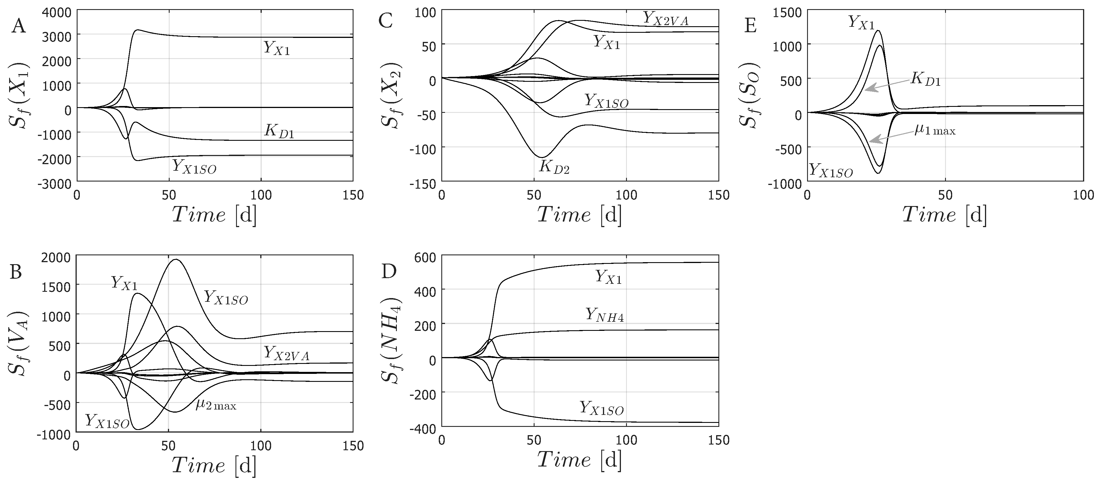
Appendix B presents a parametric sensitivity analysis of the AD-OFMSW model. The analysis identifies six coefficients with a dominant influence on the biomass states. These are the death coefficients and and the yield coefficients , , , and . The coefficient affects the ammonium balance but enters neither growth rate. Hence, the remaining five coefficients are perturbed in the simulated plant, while the EKF observer (7)–(10) and the PI controller (13) retain their nominal values. The reference profile, inlet perturbation, and initial conditions are unchanged. Only the intermediate designs A2, S2, and T2 are evaluated, one per tuning family. This selection keeps the three methods represented in the mismatch study. Design S2 is additionally one of the two balanced designs identified in Section 3.2.
The adopted mismatch scenario applies staircase deviations of and to the five coefficients. Each coefficient follows a piecewise-constant profile synchronized with the steps of the inlet perturbation. This scenario represents moderate systematic uncertainty in the stoichiometric and death coefficients. Figure 10 shows the perturbed parameter profiles. Figure 11 shows the closed-loop responses of the three designs. Table 9 summarizes the tracking and process metrics.
Figure 10.
Perturbed parameter profiles: staircase deviations of in the first two steps and of in the last two, synchronized with the inlet perturbation.
Figure 11.
Closed-loop responses under the plant–model mismatch of Figure 10. (A–C) Dilution rate for designs T1, T2, and T3, from top to bottom. (D–F) True acidogenic biomass (black solid line), its estimate (blue solid line), and its reference (dashed line) for the same designs. (G–I) Methane production rate in d−1.
Table 9.
Plant–model mismatch in the death and yield coefficients (staircase deviations of and ). and are computed on and , respectively. The biomass band residence is the percentage of time for which remains within the band mg/L. The NOC residence is the percentage of time with and . The mean is the time-weighted average, computed as .
The true-state IAE of design S2 increased from 459.5 to 1783.5 mg d/L. In contrast, the estimated-state IAE remained nearly unchanged, at 558.4 mg d/L. This gap confirms that the nominally tuned observer does not detect a stoichiometric mismatch. The controller regulates the estimate accurately, while the true biomass departs from the reference. Even under this bias, the true biomass remained within the biomass band during the whole horizon. The NOC residence was 100% in the three designs (Table 9). Moreover, the effluent substrate, volatile fatty acids, and methane production stayed close to their nominal trajectories.
These results delimit the scope of the proposed scheme. A systematic parameter bias degrades the tracking of the true biomass. The nominal observer does not detect it, because its model matches the controller design. Nevertheless, the process variables remain close to the NOC, with 100% NOC residence in the three tested designs (Table 9). A robust or adaptive observer is required to handle parametric mismatch during operation. This extension is identified as a direction for future work in Section 4.
4. Conclusions
This work proposed an observer-based PI control scheme for the anaerobic digestion of the soluble organic fraction of municipal solid waste under inhibition conditions. The main conclusions are summarized as follows.
- An extended Kalman filter reconstructed the acidogenic biomass from the online measurement of the soluble organic substrate. The estimates converged under initial offsets of up to 35% and a time-varying feed concentration. The observer operates as a soft sensor for a variable that is not measurable in practice. However, its reliability is limited to near-nominal parameters. Under a stoichiometric mismatch of , the estimated state tracked the reference, while the true-state error increased by a factor of four. Robust or adaptive observers are required to detect and compensate for this class of mismatch.
- The observer-based PI controller maintained the process around its inhibited nominal operating condition. Nine designs from three tuning methods tracked the reference and rejected the feed perturbation over a 1000 d horizon. The evaluation was limited to inlet substrate disturbances. The prevention of acidification under increased influent ammonium or reduced methanogenic activity is identified as future work. The comparison of the IAE, stability margins, and total variation revealed a clear trade-off between tracking performance, robustness, and control effort. The fastest design achieved the lowest estimated-state IAE, 501.1 mg d/L, but exhibited the lowest gain margin, 5.8 dB. The lowest true-state IAE, 450.2 mg d/L, corresponded to a design with a phase margin of . Conversely, the most conservative designs paired the largest IAE values with the largest gain margins, up to 15.2 dB. The most balanced designs combined a phase margin near with a gain margin in the recommended range and a competitive IAE. The phase margin alone did not determine this balance: design T3, with , exhibited the largest IAE of its family.
- The convergence analysis established the ultimate boundedness of the estimation error. Moreover, the closed-loop trajectories remained locally ultimately bounded under the estimation error. These properties support the theoretical consistency of the proposed scheme.
- The scheme relies on a standard analytical measurement and on a linear controller. Hence, its implementation is plausible at the laboratory and pilot scale. Transfer to full-scale plants requires the experimental validations identified as future work. In practical terms, the controller adjusts the daily feed flow to between and of the reactor volume. Future work will address the experimental calibration of the model against reactor data, the experimental validation of the scheme, and its extension to robust and adaptive tuning strategies. A quantitative comparison with other observer families, such as the asymptotic observer of Ref. [56], and a comparison with nonlinear control strategies are also planned.
Supplementary Materials
The following supporting information can be downloaded at https://www.mdpi.com/article/10.3390/fermentation12110507/s1. Figure S1: Open-loop trajectory of the AD–OFMSW model under the nominal inlet concentration mg/L, with d−1. (A) Acidogenic biomass and methanogenic biomass . (B) Soluble substrate , volatile fatty acids , and ammonium ; Figure S2: Closed-loop responses of the true-state PI benchmark. Rows: AMIGO-scaled designs (top), SIMC designs (middle), and auto-tuning designs (bottom). (A)–(C) Dilution rate ; (D)–(F) true biomass and reference (dashed); (G)–(I) methane production rate in d−1. Red: most aggressive design of each family; black: intermediate design; blue: smoothest design; Figure S3: Case 1 ( biased downward, biased upward). Perturbed parameter profiles: in the first two steps and in the last two, synchronized with the inlet perturbation; Figure S4: Case 1 ( biased downward, biased upward). Closed-loop responses of the intermediate designs A2 (top), S2 (middle), and T2 (bottom). (A)–(C) Dilution rate ; (D)–(F) true biomass (black) and its estimate (blue); (G)–(I) methane production rate in d−1; Figure S5: Case 2 (reversed signs: biased upward, biased downward). Perturbed parameter profiles: in the first two steps and in the last two, synchronized with the inlet perturbation; Figure S6: Case 2 (reversed signs: biased upward, biased downward). Closed-loop responses of the intermediate designs A2 (top), S2 (middle), and T2 (bottom). (A)–(C) Dilution rate ; (D)–(F) true biomass (black) and its estimate (blue); (G)–(I) methane production rate in d−1; Table S1: IAE index and total variation of the dilution rate for the nine true-state PI designs over the 1000 d horizon. Designs 1–3 correspond to A1–A3 (AMIGO-scaled), S1–S3 (SIMC), and T1–T3 (auto-tuning); Table S2: Tracking and process metrics for the kinetic mismatch cases. and are computed on and . The NOC residence is the percentage of time that remains within the band mg/L.
Author Contributions
Conceptualization, software, validation, formal analysis, resources, data curation, writing—original draft preparation, supervision, and project administration, R.A.F.-E.; investigation, methodology, visualization, and writing—review and editing, A.C.-S., J.M.E.H.-M., J.L.C., H.A.N.-A., R.F.G.-H., V.A.-G., and R.A.F.-E. All authors have read and agreed to the published version of the manuscript.
Funding
This research received no external funding.
Institutional Review Board Statement
Not applicable.
Informed Consent Statement
Not applicable.
Data Availability Statement
The original contributions presented in this study are included in the article and the Supplementary Materials. The simulation files and parameter sets are available from the corresponding author upon request.
Acknowledgments
We acknowledge the Computational Chemistry Laboratory at the Polytechnic University of Tapachula for partial access to computational resources.
Conflicts of Interest
The authors declare no conflicts of interest.
Abbreviations
The following abbreviations are used in this manuscript:
| ACC | Acidification condition |
| AD | Anaerobic digestion |
| ADM1 | IWA Anaerobic Digestion Model No. 1 |
| AMIGO | Approximate M-constrained integral gain optimization |
| EKF | Extended Kalman filter |
| GM | Gain margin |
| IAE | Integral of absolute error |
| MPC | Model predictive control |
| NOC | Normal operating condition |
| OFMSW | Organic fraction of municipal solid waste |
| PI | Proportional–integral |
| PM | Phase margin |
| SIMC | Skogestad internal model control |
| WSC | Washout condition |
Appendix A. Convergence Analysis of the Observer-Based Control Scheme
This appendix presents the convergence analysis of the proposed observer-based control scheme. The boundedness of the EKF estimation error is addressed first. Then, the local stability of the closed-loop system is established. The analysis is local and considers a constant admissible reference. Measurement and process noise do not enter the deterministic convergence proof; they are handled through covariance tuning. Saturation is excluded near the equilibrium, as shown in Remark A3. The gap between these hypotheses and the simulated implementation is discussed in Remark A5.
Appendix A.1. Boundedness of the EKF Estimation Error
The convergence of the EKF is analyzed under the following assumptions. These assumptions are physically realizable for the AD-OFMSW process.
Assumption A1.
The state trajectories of system (1) evolve in a compact set . The compact set Ω follows from mass conservation and contains a neighborhood of the NOC equilibrium within .
Assumption A2.
The vector field is smooth in Ω. Therefore, it is locally Lipschitz, i.e., with .
Assumption A3.
The pair is uniformly detectable along the estimated trajectories. In addition, with and with .
Remark A1.
The detectability requirement of Assumption A3 is verified only locally. At the NOC equilibrium, the pair of the linearized model has one unobservable mode at d−1, which is strictly stable. The uniform detectability of the time-varying pair along the estimated trajectories is assumed, not proven. The simulations of Section 3.1 are consistent with this assumption in the tested scenarios, but they do not verify it.
Remark A2.
Under Assumption A3, the solution of the Riccati Equation (9) is bounded. In particular, , with .
Assumption A4.
The higher-order terms of the Taylor expansion of f are bounded. In particular, for , with and .
The estimation error is defined as . From Equations (1) and (7), the error dynamics are
where collects the higher-order terms of the Taylor expansion of f.
Lemma A1.
Proof.
Consider the following Lyapunov candidate function:
From the bounds of , the function satisfies . The time derivative of (A2) along the trajectories of (A1) is
Then, from Assumptions A3 and A4,
Note that is only positive semidefinite, since a single output is measured. Nevertheless, the term is positive definite and dominates the higher-order term in a neighborhood of the origin. Indeed, from (A5), whenever , with . Since , the level set is contained in this ball and is positively invariant. Hence, guarantees that the error remains bounded for all . Standard ultimate boundedness arguments then yield for some [80]. □
Appendix A.2. Local Stability of the Closed-Loop System
The local stability of the closed-loop system is now analyzed. The analysis combines Lemma A1 with the local stability of the NOC equilibrium reported in [41]. Since is an open set that contains in its interior, sufficiently small neighborhoods of the equilibrium remain within the operating region, which justifies the local analysis. The tracking error can be decomposed as
where is the first entry of the estimation error . Let denote the integrator state of the controller (13), i.e., . Then, the control law reads as . The nominal closed-loop system is obtained for :
Note that the model (1) is affine in the dilution rate D. Hence, the estimation error enters the closed-loop dynamics in an exact form, through the proportional action and through the integrator state:
where .
Assumption A5.
The reference is admissible, i.e., the corresponding steady-state dilution rate satisfies . Moreover, the gains and are selected such that the linearization of (A7) at the equilibrium associated with is Hurwitz.
This property has been verified numerically for the nine designs of Section 3.2. The linearization of (A7) at the equilibrium associated with mg/L yields eigenvalues with strictly negative real parts in all cases. The rightmost eigenvalue is d−1 in every design. It coincides with the stable unobservable ammonium mode of Section 2.2, which the feedback does not move. The dominant controlled poles range from d−1 (T3) to d−1 (T2). The dominant closed-loop poles are reported in Table A1.
Remark A3.
Under Assumption A5, the saturation block is inactive near the equilibrium. Therefore, the local analysis remains valid.
Proposition A1.
Consider the closed-loop system (20) driven by the EKF observer (7)–(10). Under Assumptions A1–A5, let the initial conditions be sufficiently close to the equilibrium associated with , and let the initial estimation error satisfy . Then, the closed-loop trajectories are locally ultimately bounded. Moreover, the regulation error converges to a neighborhood of the origin. The radius of this neighborhood is proportional to the estimation error bound ρ.
Proof.
By Assumption A5 and the indirect Lyapunov method, the nominal system (A7) is locally exponentially stable. A locally exponentially stable system is locally input-to-state-stable with respect to bounded perturbations [73,80]. The perturbation term is bounded, since the entries of G depend affinely on , which remains in , and . By Lemma A1, is ultimately bounded by . Therefore, the trajectories of z are locally ultimately bounded. Finally, the integral action of the nominal loop enforces when . The regulation error thus converges to a neighborhood of the origin with a radius proportional to . □
Table A1.
Closed-loop eigenvalues of the linearization of (A7) at the equilibrium associated with mg/L. Dominant poles; all remaining poles have more negative real parts. The rightmost eigenvalue is d−1 in every design.
Remark A4.
The stability result is local, which is consistent with the local stability of the NOC equilibrium [41]. The EKF does not guarantee the asymptotic convergence of the estimation error. However, the ultimate bound ρ can be reduced during observer tuning by increasing q or decreasing r. In the six open-loop scenarios of Section 3.1, the steady-state floors of range from to mg/L. Hence, within the tested class, the ultimate bound is empirically bounded by mg/L. The convergence band mg/L of Section 3.1 is set at times this largest floor.
Remark A5.
Proposition A1 is a deterministic local result. Its hypotheses exclude measurement and process noise, time-varying references, and active saturation. The simulations of Section 3.2 include all these effects. These simulations are finite-horizon numerical observations. They are consistent with the proven result, but they are not covered by it. In particular, Proposition A1 does not establish ultimate boundedness under stochastic noise or active saturation. The input-to-state interpretation of the proof suggests that small bounded perturbations preserve boundedness close to the equilibrium. A formal treatment of time-varying references, stochastic noise, and active saturation is identified as future work.
Appendix B. Parametric Sensitivity Analysis
To identify the parameters that significantly influence the dynamical behavior of the AD-OFMSW model, a parametric sensitivity analysis is performed. The analysis follows the forward sensitivity framework for chemical systems [80,81]. The sensitivity functions are computed by the simultaneous solution of the AD-OFMSW model and the following equation:
Figure A1 shows the numerical solution of Equation (A9) for the eight kinetic and stoichiometric parameters of the model. At steady state, the sensitivity functions converge to constant values. The non-negligible stationary sensitivities of the biomass states involve the death and yield coefficients , , , , and . The maximum growth rates and exhibit large transient sensitivities but vanish at steady state. This behavior arises from the steady-state identity at the NOC. The coefficient only influences the ammonium balance, and the sensitivities of converge to zero for all parameters. The reported sensitivities are dimensional by construction, following the forward sensitivity framework of Refs. [80,81]. Normalized sensitivities constitute a complementary analysis that is identified as future work. These coefficients are perturbed in the plant–model mismatch evaluation of Section 3.3.
Figure A1.
Solution of the sensitivity equation (Equation (A9)). Sensitivities of (A) , (B) , (C) , (D) , and (E) with respect to the parameter set (only the most sensitive are labeled).
References
- Alcaraz–Gonzalez, V.; Flores–Estrella, R.A.; Haarstrick, A.; Gonzalez–Alvarez, V. Wastewater exploitation from microbiological activity to energy. In Springer Water; Kostianoy, A.G., Shirshov, P.P., Eds.; Springer Nature: Cham, Switzerland, 2024. [Google Scholar]
- Zamri, M.F.M.A.; Hasmady, S.; Akhiar, A.; Ideris, F.; Shamsuddin, A.H.; Mofijur, M.; Fattah, I.M.R.; Mahlia, T.M.I. A comprehensive review on anaerobic digestion of organic fraction of municipal solid waste. Renew. Sustain. Energy Rev. 2021, 137, 110637. [Google Scholar] [CrossRef] [Scilit]
- Barampouti, E.M.; Mai, S.; Malamis, D.; Moustakas, K.; Loizidou, M. Liquid biofuels from the organic fraction of municipal solid waste: A review. Renew. Sustain. Energy Rev. 2019, 110, 298–314. [Google Scholar] [CrossRef] [Scilit]
- Colelli, L.; Verdone, N.; Segneri, V.; Vilardi, G. Dynamic analysis of the oxidative coupling of methane (OCM) process to produce sustainable ethylene from biogas derived from organic fraction of municipal solid waste (OFMSW). Biomass Bioenergy 2025, 203, 108345. [Google Scholar] [CrossRef] [Scilit]
- Pérez–Roman, A.; Lopez-Arenas, T.; Sales-Cruz, M.; Rocha-Rios, J. Simulation of a biorefinery process from the organic fraction of municipal solid waste generated in México City. J. Chem. Technol. Biotechnol. 2025, 100, 2053–2064. [Google Scholar] [CrossRef] [Scilit]
- Panigrahi, S.; Dubey, B.K. A critical review on operating parameters and strategies to improve the biogas yield from anaerobic digestion of organic fraction of municipal solid waste. Renew. Energy 2019, 143, 779–797. [Google Scholar] [CrossRef] [Scilit]
- Francesca, D.; Elisa, R.; Alessandro, D.F.; Emilio, M.; Tonia, T.; Debora, F. Modelling of technical, environmental, and economic evaluations of the effect of the organic loading rate in semi-continuous anaerobic digestion of pre-treated organic fraction municipal solid waste. Environ. Pollut. 2024, 344, 123417. [Google Scholar] [CrossRef] [Scilit] [PubMed]
- Pavi, S.; Kramer, L.E.; Gomes, L.P.; Miranda, L.A.S. Biogas production from co-digestion of organic fraction of municipal solid waste and fruit and vegetable waste. Bioresour. Technol. 2017, 228, 362–367. [Google Scholar] [CrossRef] [Scilit] [PubMed]
- Pavan, P.; Battistoni, P.; Cecchi, F.; Mata–Alvarez, J. Two-phase anaerobic digestion of source sorted OFMSW (organic fraction of municipal solid waste): Performance and kinetic study. Water Sci. Technol. 2000, 41, 111–118. [Google Scholar] [CrossRef] [Scilit]
- Bala, R.; Gupta, G.K.; Dasgupta, B.V.; Mondal, M.K. Pretreatment optimisation and kinetics of batch anaerobic digestion of liquidised OFMSW treated with NaOH: Models verification with experimental data. J. Environ. Manag. 2019, 237, 313–321. [Google Scholar] [CrossRef] [Scilit] [PubMed]
- Pulgarín–Muñoz, C.E.; Saldarriaga–Molina, J.C.; Castro–Valencia, J.C.; Correa–Ochoa, M.A.; Echeverry–Ruiz, J.D. Effect of the co-substrate ratio on the anaerobic co–digestion of sewage sludge and the organic fraction of municipal solid waste at pilot scale. Int. Biodeterior. Biodegrad. 2025, 198, 106008. [Google Scholar] [CrossRef] [Scilit]
- Abbas, R.I.; Flayeh, H.M. Aerobic composting of organic waste, alternative and an efficient solid waste management solution. Asian J. Water Environ. Pollut. 2024, 21, 101–111. [Google Scholar] [CrossRef] [Scilit]
- Haque, N.; Azad, A. Comparative study of hydrogen production from organic fraction of municipal solid waste and its challenges: A review. Energies 2023, 16, 7853. [Google Scholar] [CrossRef] [Scilit]
- El Hadj, T.B.; Astals, S.; Galí, A.; Mace, S.; Mata–Alvarez, J. Ammonia influence in anaerobic digestion of OFMSW. Water Sci. Technol. 2009, 59, 1153–1158. [Google Scholar] [CrossRef] [Scilit] [PubMed]
- Li, L.; Peng, X.Y.; Wang, X.M.; Di Wu, D. Anaerobic digestion of food waste: A review focusing on process stability. Bioresour. Technol. 2018, 248, 20–28. [Google Scholar] [CrossRef] [Scilit] [PubMed]
- Hill, D.T.; Barth, C.L. A dynamic model for simulation of animal waste digestion. J. Water Pollut. Control Fed. 1977, 49, 2129–2143. [Google Scholar]
- Kiely, G.; Tayfur, G.; Dolan, C.; Tanji, K. Physical and mathematical modelling of anaerobic digestion of organic wastes. Water Res. 1997, 31, 534–540. [Google Scholar] [CrossRef] [Scilit]
- Havlik, I.; Voturba, J.; Sobotka, M. Mathematical modeling of the anaerobic digestion process: Application of dynamic mass-energy balance. Folia Microbiol. 1986, 31, 56–68. [Google Scholar] [CrossRef] [Scilit]
- Moletta, R.; Verrier, D.; Albagnac, G. Dynamic modelling of anaerobic digestion. Water Res. 1986, 20, 427–434. [Google Scholar] [CrossRef] [Scilit]
- Cecchi, F.; Mata–Alvarez, J.; Marcomini, A.; Pavan, P. First order and step-diffusional kinetic models in simulating the mesophilic anaerobic digestion of complex substrates. Bioresour. Technol. 1991, 36, 261–269. [Google Scholar] [CrossRef] [Scilit]
- Cecchi, F.; Pavan, P.; Mata–Alvarez, J. Kinetic study of the thermophilic anaerobic digestion of the fresh and precomposted, mechanically selected, organic fraction of municipal solid waste. J. Environ. Sci. Health Part A 1997, 32, 195–213. [Google Scholar]
- Batstone, D.J.; Keller, J.; Angelidaki, I.; Kalyuzhnyi, S.V.; Pavlostathis, S.G.; Rozzi, A.; Sanders, W.T.M.; Siegrist, H.; Vavilin, V.A. The IWA anaerobic digestion model no 1 (ADM1). Water Sci. Technol. 2002, 45, 65–73. [Google Scholar] [CrossRef] [Scilit]
- Batstone, D.J.; Puyol, D.; Flores–Alsina, X.; Rodriguez, J. Mathematical modelling of anaerobic digestion processes: Applications and future needs. Rev. Environ. Sci. Biotechnol. 2015, 14, 595–613. [Google Scholar] [CrossRef] [Scilit]
- Mo, R.R.; Guo, W.J.; Batstone, D.; Makinia, J.; Li, Y.M. Modifications to the anaerobic digestion model no. 1 (ADM1) for enhanced understanding and application of the anaerobic treatment processes—A comprehensive review. Water Res. 2023, 244, 120504. [Google Scholar] [CrossRef] [Scilit] [PubMed]
- Esposito, G.; Frunzo, L.; Panico, A.; d’Antonio, G. Mathematical modelling of disintegration–limited co–digestion of OFMSW and sewage sludge. Water Sci. Technol. 2008, 58, 1513–1519. [Google Scholar] [CrossRef] [Scilit] [PubMed]
- Esposito, G.; Frunzo, L.; Panico, A.; Pirozzi, F. Model calibration and validation for OFMSW and sewage sludge co–digestion reactors. Waste Manag. 2011, 31, 2527–2535. [Google Scholar] [CrossRef] [Scilit] [PubMed]
- Esposito, G.; Frunzo, L.; Panico, A.; Pirozzi, F. Modelling the effect of the OLR and OFMSW particle size on the performances of an anaerobic co–digestion reactor. Process Biochem. 2011, 46, 557–565. [Google Scholar] [CrossRef] [Scilit]
- Pastor–Poquet, V.; Papirio, S.; Steyer, J.P.; Trably, E.; Escudie, R.; Esposito, G. High–solids anaerobic digestion model for homogenized reactors. Water Res. 2018, 142, 501–511. [Google Scholar] [CrossRef] [Scilit] [PubMed]
- Pastor–Poquet, V.; Papirio, S.; Steyer, J.P.; Trably, E.; Escudie, R.; Esposito, G. Modelling non–ideal bio–physical–chemical effects on high–solids anaerobic digestion of the organic fraction of municipal solid waste. J. Environ. Manag. 2019, 238, 408–419. [Google Scholar] [CrossRef] [Scilit] [PubMed]
- Pastor–Poquet, V.; Papirio, S.; Harmand, J.; Steyer, J.P.; Trably, E.; Escudie, R.; Esposito, G. Assessing practical identifiability during calibration and cross-validation of a structured model for high-solids anaerobic digestion. Water Res. 2019, 164, 114932. [Google Scholar] [CrossRef] [Scilit] [PubMed]
- Yu, L.; Zhao, Q.B.; Ma, J.W.; Frear, C.; Chen, S.L. Experimental and modeling study of a two-stage pilot scale high solid anaerobic digester system. Bioresour. Technol. 2012, 124, 8–17. [Google Scholar] [CrossRef] [Scilit] [PubMed]
- Bollon, J.; Le–Hyaric, R.; Benbelkacem, H.; Buffiere, P. Development of a kinetic model for anaerobic dry digestion processes: Focus on acetate degradation and moisture content. Biochem. Eng. J. 2011, 56, 212–218. [Google Scholar] [CrossRef] [Scilit]
- Gao, Q.W.; Li, L.L.; Wang, K.; Zhao, Q.L. Mass transfer enhancement in high-solids anaerobic digestion of organic fraction of municipal solid wastes: A review. Bioengineering 2023, 10, 1084. [Google Scholar] [CrossRef] [Scilit] [PubMed]
- Roeva, O.; Chorukova, E.; Kabaivanova, L. Advanced mathematical modeling of hydrogen and methane production in a two-stage anaerobic co-digestion system. Mathematics 2025, 13, 1601. [Google Scholar] [CrossRef] [Scilit]
- Berga, H.; Alla, A.; El Khattabi, N. Mathematical analysis of an anaerobic co-digestion model with preference function and mortality. Math. Meth. Appl. Sci. 2023, 46, 10103–10122. [Google Scholar] [CrossRef] [Scilit]
- Ahlamine, I.; Alla, A.; El Khattabi, N. Mathematical analysis of an anaerobic digestion model for biogas production from solid waste. Sci. Rep. 2024, 14, 25934. [Google Scholar] [CrossRef] [Scilit] [PubMed]
- Xie, S.H.; Hai, F.I.; Zhan, X.M.; Guo, W.S.; Ngo, H.H.; Price, W.E.; Nghiem, L.D. Anaerobic co–digestion: A critical review of mathematical modelling for performance optimization. Bioresour. Technol. 2016, 222, 498–512. [Google Scholar] [CrossRef] [Scilit] [PubMed]
- Silva, T.P.; dos Santos, A.B.; Esposito, G.; Gehring, T.A.; Leitao, R.C. Bibliometric analysis of anaerobic digestion model no. 1 for dry anaerobic digestion of fruit and vegetable waste, food waste, and organic fraction of municipal solid waste. J. Environ. Chem. Eng. 2024, 12, 114664. [Google Scholar] [CrossRef] [Scilit]
- Yang, Z.; Larsen, O.C.; Muhayodin, F.; Hu, J.W.; Xue, B.; Rotter, V.S. Review of anaerobic digestion models for organic solid waste treatment with a focus on the fates of C, N, and P. Energy Ecol. Environ. 2025, 10, 1–14. [Google Scholar] [CrossRef] [Scilit]
- Kegl, T.; Jiménez, E.T.; Kegl, B.; Kralj, A.K.; Kegl, M. Modeling and optimization of anaerobic digestion technology: Current status and future outlook. Prog. Energy Combust. Sci. 2025, 106, 101199. [Google Scholar] [CrossRef] [Scilit]
- Flores–Estrella, R.A.; Gutiérrez–Hernández, R.F.; Nágera–Aguilar, H.A.; Castañon–Gonzalez, J.H.; Cabellos, J.L.; Ríos–Valdovinos, E.; Cruz–Salomón, A. Anaerobic Digestion of Soluble Organic Fraction of Municipal Solid Waste Under Inhibition Conditions: Analysis and Control. Processes 2026, 14, 855. [Google Scholar] [CrossRef] [Scilit]
- Flores–Estrella, R.A.; Estrada–Baltazar, A.; Femat, R. A mathematical model and dynamic analysis of anaerobic digestion of soluble organic fraction of municipal solid waste towards control design. Rev. Mex. Ing. Quim. 2016, 15, 243–258. [Google Scholar]
- Jimenez, J.; Latrille, E.; Harmand, J.; Robles, A.; Ferrer, J.; Gaida, D.; Wolf, C.; Mairet, F.; Bernard, O.; Alcaraz-Gonzalez, V.; et al. Instrumentation and control of anaerobic digestion processes: A review and some research challenges. Rev. Environ. Sci. Biotechnol. 2015, 14, 615–648. [Google Scholar] [CrossRef] [Scilit]
- Nguyen, D.; Gadhamshetty, V.; Nitayavardhana, S.; Khanal, S.K. Automatic process control in anaerobic digestion technology: A critical review. Bioresour. Technol. 2015, 193, 513–522. [Google Scholar] [CrossRef] [Scilit] [PubMed]
- Gaida, D.; Wolf, C.; Bongards, M. Feed control of anaerobic digestion processes for renewable energy production: A review. Renew. Sustain. Energy Rev. 2017, 68, 869–875. [Google Scholar] [CrossRef] [Scilit]
- Ortega–Muñan, W.E.; Flores–Estrella, R.A.; Torres–Zúñiga, I.; Alcaraz–Gonzalez, V. Stabilization of two-stage anaerobic bioreactors via Port-Hamiltonian passive control. J. Process Control 2026, 166, 103812. [Google Scholar] [CrossRef] [Scilit]
- Méndez–Acosta, H.O.; Palacios–Ruiz, B.; Alcaraz–González, V.; González–Alvarez, V.; García–Sandoval, J.P. A robust control scheme to improve the stability of anaerobic digestion processes. J. Process Control 2010, 20, 375–383. [Google Scholar] [CrossRef] [Scilit]
- Flores–Estrella, R.A.; Colin Robles, J.J.; Torres–Zúñiga, I.; López–Caamal, F.; Alcaraz–Gonzalez, V. Robust Substrate Control for a Microbial Electrolysis Cell System. Processes 2026, 14, 1876. [Google Scholar] [CrossRef] [Scilit]
- Lara–Cisneros, G.; Aguilar–López, R.; Femat, R. On the dynamic optimization of methane production in anaerobic digestion via extremum-seeking control approach. Comput. Chem. Eng. 2015, 75, 49–59. [Google Scholar] [CrossRef] [Scilit]
- Cortés, L.G.; Barbancho, J.; Larios, D.F.; Marin–Batista, J.D.; Mohedano, A.F.; Portilla, C.; de la Rubia, M.A. Full-scale digesters: Model predictive control with online kinetic parameter identification strategy. Energies 2022, 15, 8594. [Google Scholar] [CrossRef] [Scilit]
- Paladino, O. Data driven modelling and control strategies to improve biogas quality and production from high solids anaerobic digestion: A mini review. Sustainability 2022, 14, 16467. [Google Scholar] [CrossRef] [Scilit]
- Khan, M.; Chuenchart, W.; Surendra, K.C.; Khanal, S.K. Applications of artificial intelligence in anaerobic co-digestion: Recent advances and prospects. Bioresour. Technol. 2023, 370, 128501. [Google Scholar] [CrossRef] [Scilit] [PubMed]
- Ling, J.Y.X.; Chan, Y.J.; Chen, J.W.; Chong, D.J.S.; Tan, A.L.L.; Arumugasamy, S.K.; Lau, P.L. Machine learning methods for the modelling and optimisation of biogas production from anaerobic digestion: A review. Environ. Sci. Pollut. Res. 2024, 31, 19085–19104. [Google Scholar] [CrossRef] [Scilit] [PubMed]
- Salma, A.; Laferte, J.M.; Fryda, L.; Djelal, H. Advancing bioenergy: In-situ and in-silico approach to enhance anaerobic digestion. Waste Biomass Valorization 2025, 17, 1231–1250. [Google Scholar] [CrossRef] [Scilit]
- Simeonov, I.; Hubenov, V. Application of artificial intelligence for prediction, monitoring, optimization and control of anaerobic digestion processes—A review. Processes 2025, 13, 3812. [Google Scholar] [CrossRef] [Scilit]
- Alcaraz–González, V.; Salazar–Peña, R.; González–Alvarez, V.; Gouzé, J.L.; Steyer, J.P. A tunable multivariable nonlinear robust observer for biological systems. C. R. Biol. 2005, 328, 317–325. [Google Scholar] [CrossRef] [Scilit] [PubMed]
- Alcaraz–González, V.; Harmand, J.; Rapaport, A.; Steyer, J.P.; González–Alvarez, V.; Pelayo–Ortiz, C. Software sensors for highly uncertain WWTPs: A new approach based on interval observers. Water Res. 2002, 36, 2515–2524. [Google Scholar] [CrossRef] [Scilit] [PubMed]
- Sbarciog, M.; Moreno, J.A.; Vande Wouwer, A. Application of super-twisting observers to the estimation of state and unknown inputs in an anaerobic digestion system. Water Sci. Technol. 2014, 69, 414–421. [Google Scholar] [CrossRef] [Scilit] [PubMed]
- Rueda–Escobedo, J.G.; Sbarciog, M.; Moreno, J.A.; Van Impe, J.; Vande Wouwer, A. Robust state and input estimation with enhanced convergence rate for monitoring anaerobic digestion. J. Process Control 2022, 117, 169–180. [Google Scholar] [CrossRef] [Scilit]
- Didi, I.; Dib, H.; Cherki, B. A Luenberger-type observer for the AM2 model. J. Process Control 2015, 32, 117–126. [Google Scholar] [CrossRef] [Scilit]
- Didi, I.; Rapaport, A.; Dib, H.; Cherki, B. A positive observer for the chemostat model with biogas measurement. J. Process Control 2023, 122, 49–58. [Google Scholar] [CrossRef] [Scilit]
- Carlos–Hernandez, S.; Sanchez, E.N.; Béteau, J.F. Fuzzy observers for anaerobic WWTP: Development and implementation. Control Eng. Pract. 2009, 17, 690–702. [Google Scholar] [CrossRef] [Scilit]
- Belmonte–Izquierdo, R.; Carlos–Hernandez, S.; Sanchez, E.N. A new neural observer for an anaerobic bioreactor. Int. J. Neural Syst. 2010, 20, 75–86. [Google Scholar] [CrossRef] [Scilit] [PubMed]
- Rodríguez, A.; Quiroz, G.; Femat, R.; Méndez–Acosta, H.O.; de León, J. An adaptive observer for operation monitoring of anaerobic digestion wastewater treatment. Chem. Eng. J. 2015, 269, 186–193. [Google Scholar] [CrossRef] [Scilit]
- Draa, K.C.; Zemouche, A.; Alma, M.; Voos, H.; Darouach, M. Nonlinear observer-based control with application to an anaerobic digestion process. Eur. J. Control 2019, 45, 74–84. [Google Scholar] [CrossRef] [Scilit]
- Raeyatdoost, N.; Bongards, M.; Back, T.; Wolf, C. Robust state estimation of the anaerobic digestion process for municipal organic waste using an unscented Kalman filter. J. Process Control. 2023, 121, 50–59. [Google Scholar] [CrossRef] [Scilit]
- Hellmann, S.; Wilms, T.; Streif, S.; Weinrich, S. A tutorial to multirate extended Kalman filter design for monitoring of agricultural anaerobic digestion plants. J. Process Control 2026, 162, 103703. [Google Scholar] [CrossRef] [Scilit]
- Xu, M.C.; Jiang, Y.H.; Xu, J.J.; Fang, D. Soft sensors in anaerobic digestion: Cross-study insights, applications, and future directions. Process Biochem. 2026, 167, 74–82. [Google Scholar] [CrossRef] [Scilit]
- Aguilar–Garnica, E.; García–Sandoval, J.P.; Aceves–Lara, C.A.; Escalante, F.M.E. An asymptotic observer-based monitoring scheme for a class of plug flow reactors. Water Sci. Technol. 2012, 65, 205–213. [Google Scholar] [CrossRef] [Scilit] [PubMed]
- Simon, D. Optimal State Estimation: Kalman, H Infinity, and Nonlinear Approaches; Wiley-Interscience: Hoboken, NJ, USA, 2006. [Google Scholar]
- Reif, K.; Unbehauen, R. The extended Kalman filter as an exponential observer for nonlinear systems. IEEE Trans. Signal Process 1999, 47, 2324–2328. [Google Scholar] [CrossRef] [Scilit]
- Boutayeb, M.; Rafaralahy, H.; Darouach, M. Convergence analysis of the extended Kalman filter used as an observer for nonlinear deterministic discrete-time systems. IEEE Trans. Autom. Control 1997, 42, 581–586. [Google Scholar] [CrossRef] [Scilit]
- Zhou, K.; Doyle, J.C. Essentials of Robust Control; Prentice Hall: Saddle River, NJ, USA, 1997. [Google Scholar]
- Antsaklis, P.J.; Michel, A.N. Linear Systems; Birkhäuser: Boston, MA, USA, 2006. [Google Scholar]
- Chen, C.T. Linear System Theory and Design, 3rd ed.; Oxford University Press: New York, NY, USA, 1999. [Google Scholar]
- O’Dwyer, A. Handbook of PI and PID Controller Tuning Rules; Imperial College Press: Singapore, 2009. [Google Scholar]
- Astrom, K.J.; Hagglund, T. Advanced PID Control; Instrumentation, Systems, and Automation Society: Durham, NC, USA, 2006. [Google Scholar]
- Skogestad, S. Simple analytic rules for model reduction and PID controller tuning. J. Process Control 2003, 13, 291–309, Correction in J. Process Control 2004, 14, 465. [Google Scholar] [CrossRef] [Scilit]
- Lee, J.; Cho, W.; Edgar, T.F. Simple Analytic PID Controller Tuning Rules Revisited. Ind. Eng. Chem. Res. 2014, 53, 5038–5047. [Google Scholar] [CrossRef] [Scilit]
- Khalil, H.K. Nonlinear Systems; Prentice Hall: Upper Saddle River, NJ, USA, 2002. [Google Scholar]
- Varma, A.; Morbidelli, M.; Wu, H. Parametric Sensitivity in Chemical Systems; Cambridge University Press: Cambridge, UK, 1999. [Google Scholar]
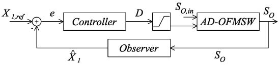
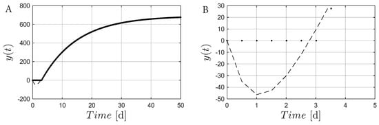
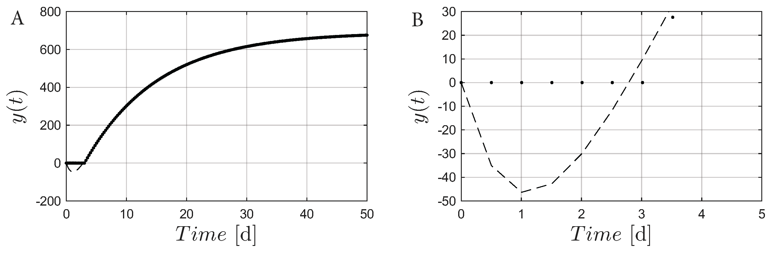
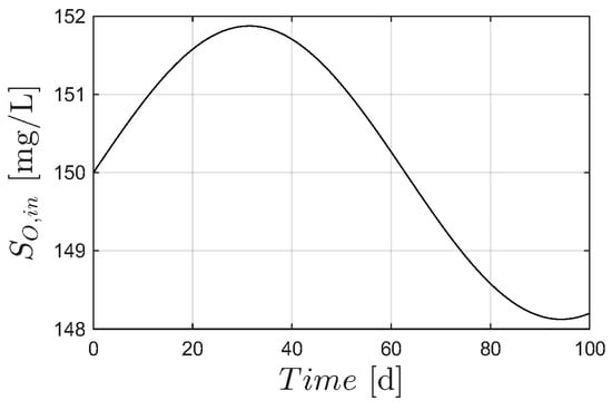
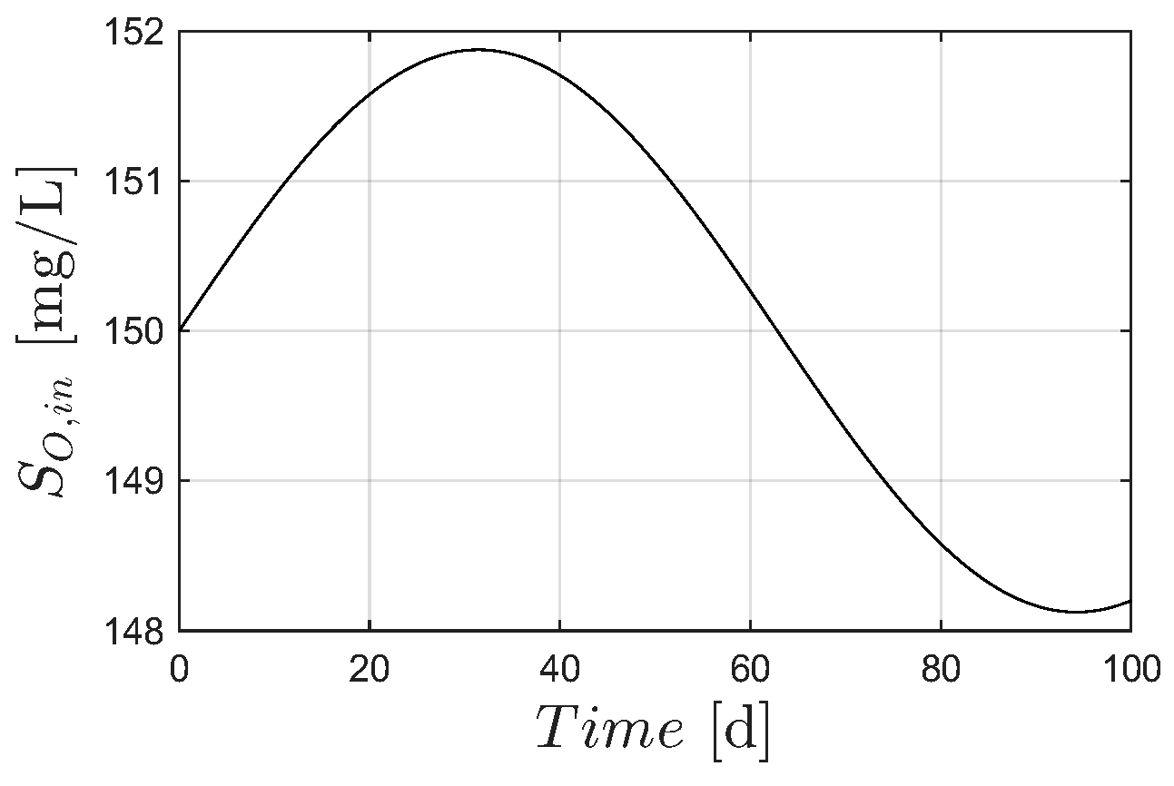
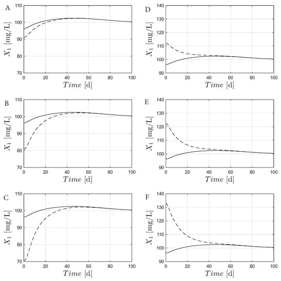
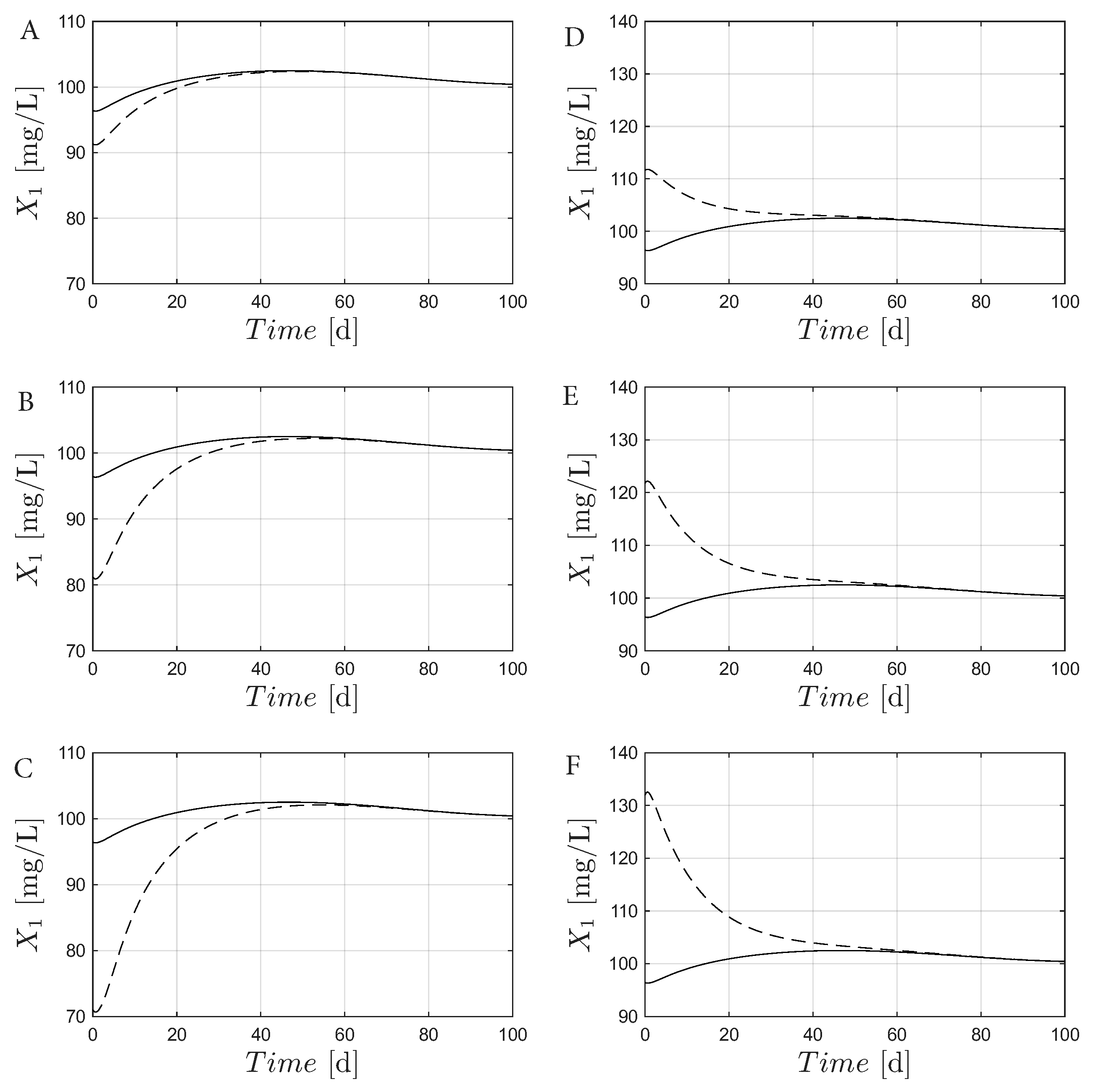
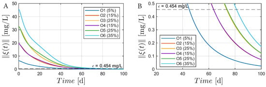
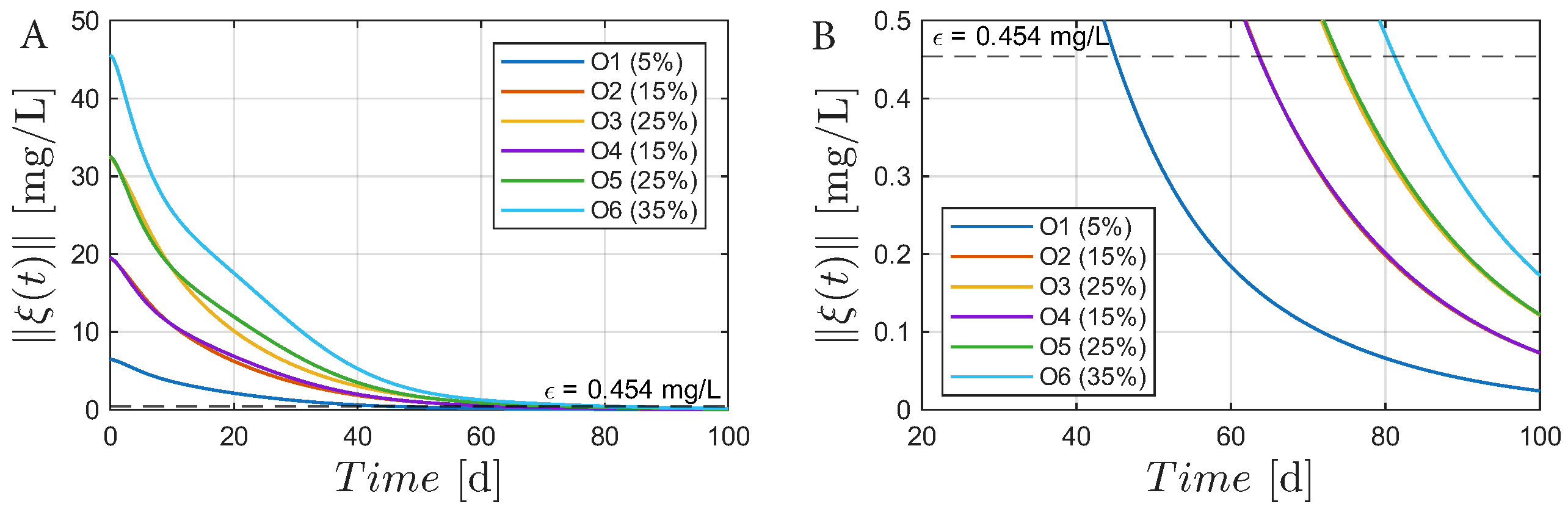
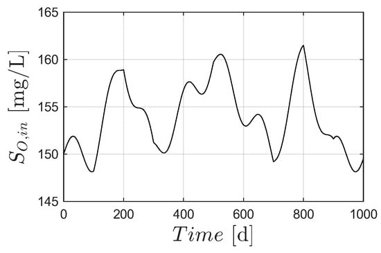
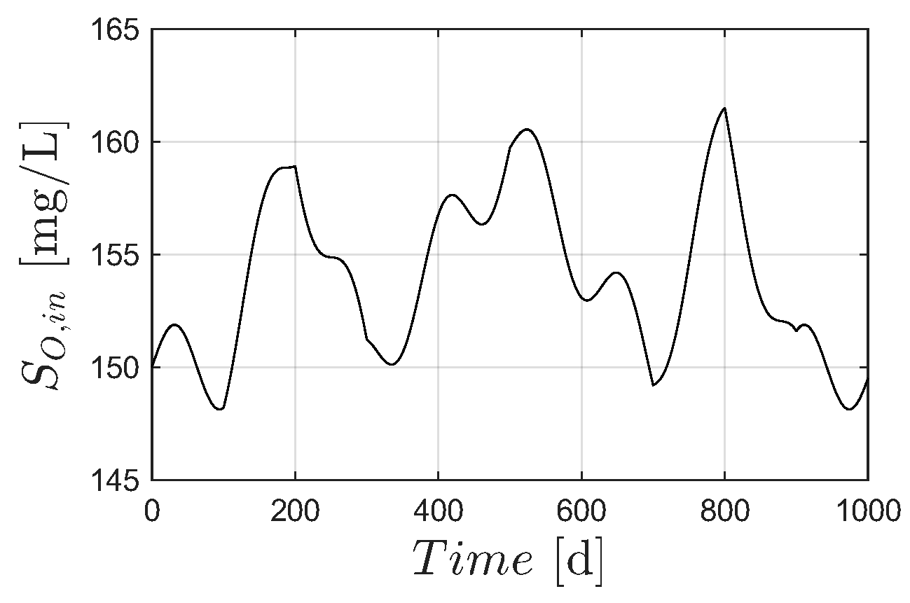
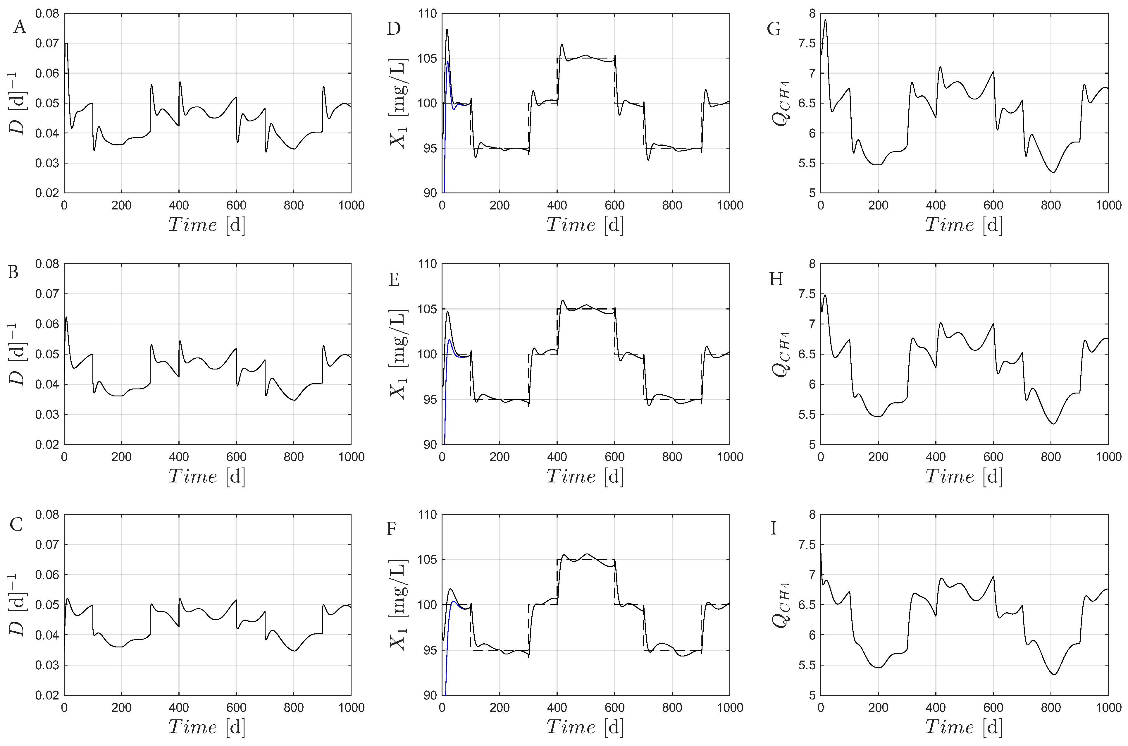
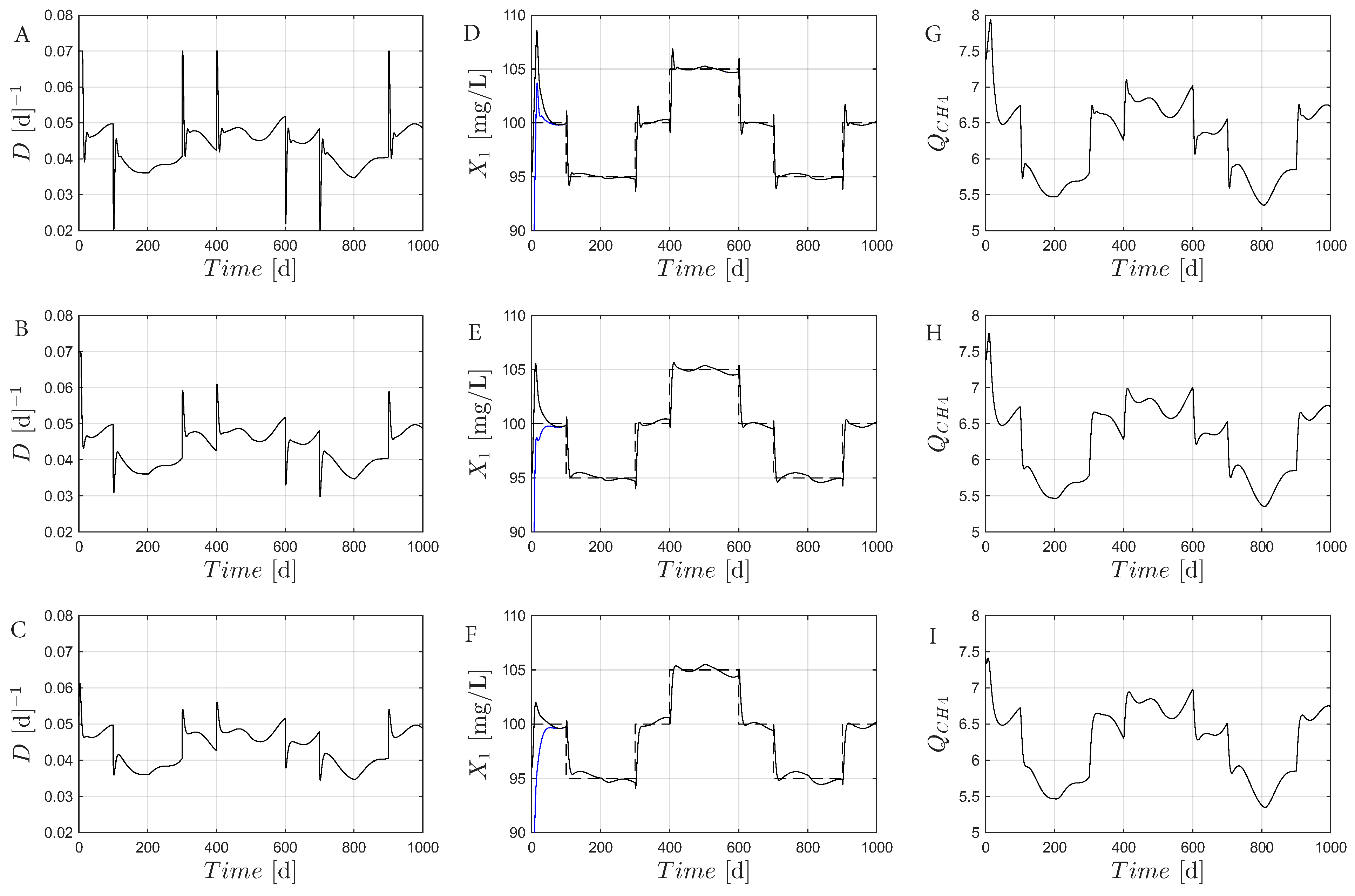
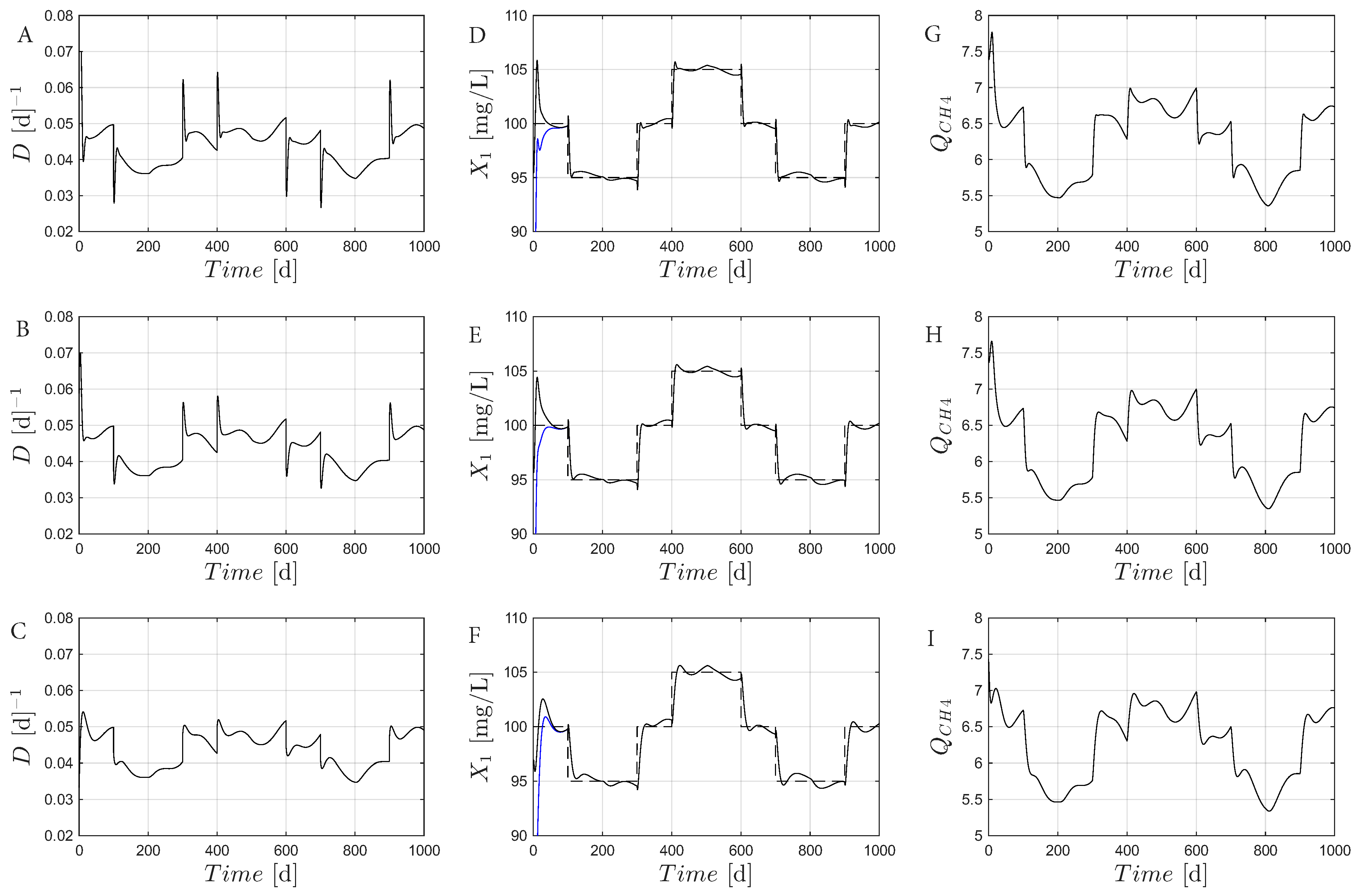
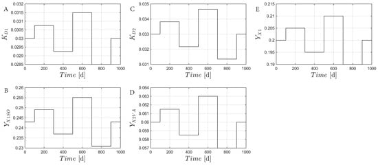
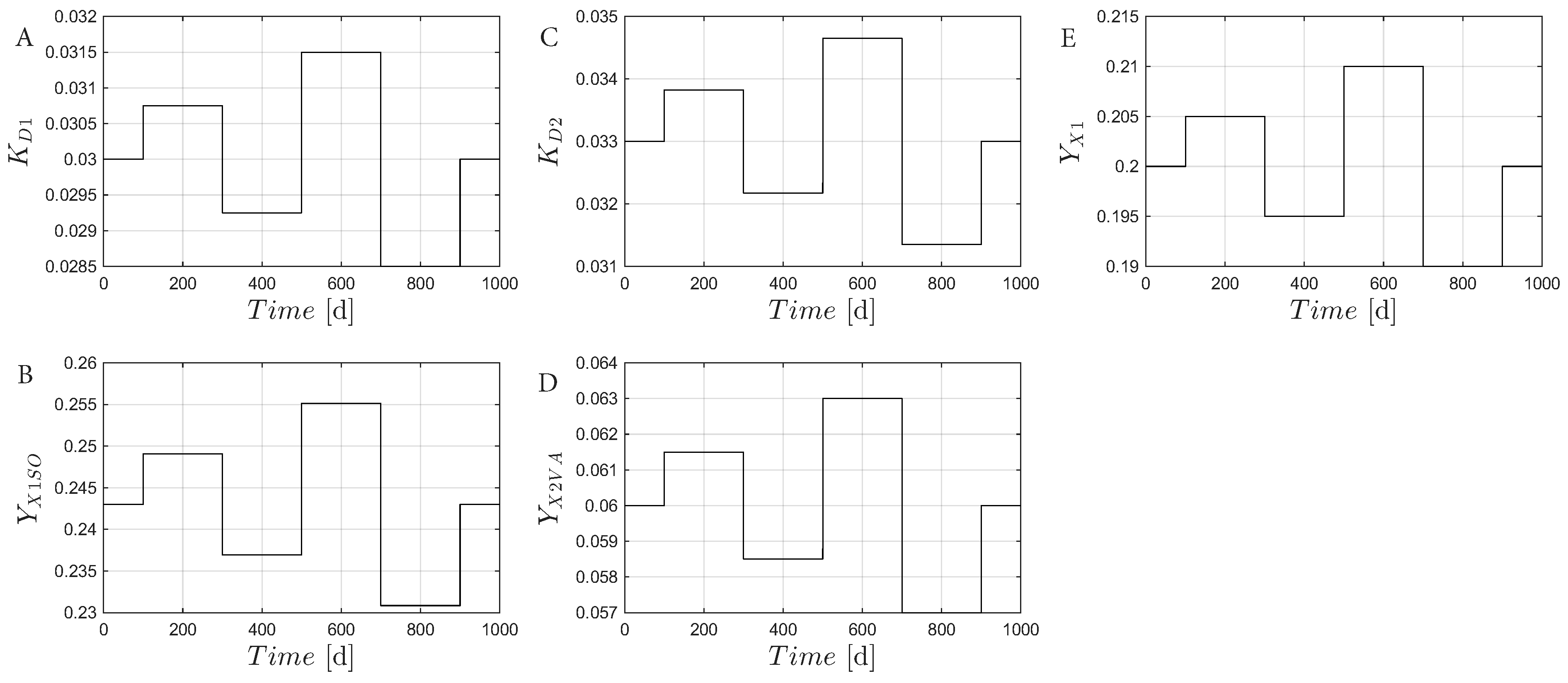
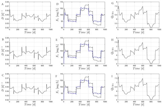
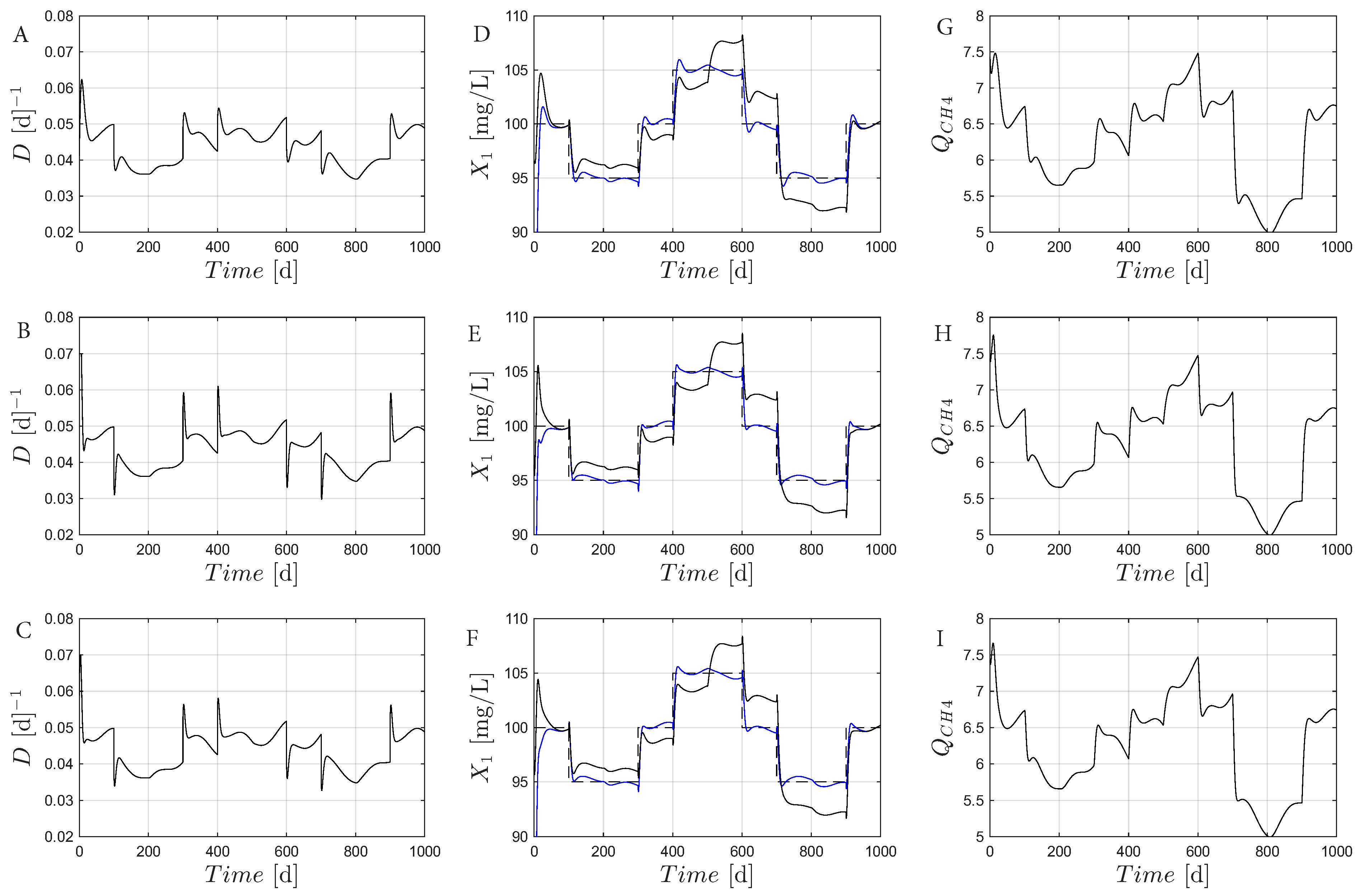

Disclaimer/Publisher’s Note: The statements, opinions and data contained in all publications are solely those of the individual author(s) and contributor(s) and not of MDPI and/or the editor(s). MDPI and/or the editor(s) disclaim responsibility for any injury to people or property resulting from any ideas, methods, instructions or products referred to in the content. |
© 2026 by the authors. Licensee MDPI, Basel, Switzerland. This article is an open access article distributed under the terms and conditions of the Creative Commons Attribution (CC BY) license.