


Abstract
Water-based suppression systems are widely employed in fire safety engineering, yet the accurate CFD modelling of their interaction with fire-driven flows remains a significant challenge. This study evaluates the impact of drag force modelling and grid mesh resolution on interaction boundary height predictions between a hot air jet at experimental velocities of 3.3, 4.2, and 5.3 ms−1 and a full-cone 30° water spray nozzle operating at 0.084 LPM using the Fire Dynamics Simulator (FDS 6.9.1), employing the Very Large Eddy Simulation (VLES) turbulence simulation mode with the Deardorff subgrid-scale and WALE near-wall turbulence models. Gas phase and water spray simulations were independently validated against the experimental measurements of Zhou, with the water spray study establishing that representative Lagrangian particles must be on the order of 105 to avoid spurious zero readings in far-field measurements. Interaction phase modelling was conducted using mesh cell sizes of 4 mm and 2 mm with a localized drag reduction approach, confirmed to operate within the LES regime through an a posteriori turbulence resolution assessment. The results demonstrate that improved drag physics combined with refined grid resolution yields meaningful improvements in the predicted interaction boundary height, highlighting the importance of addressing both aspects concurrently for reliable multi-phase flow predictions in FDS.
1. Introduction
Computational Fluid Dynamics (CFD) has become an increasingly prominent tool in fire engineering, finding application across both research and performance-based design. Modelling fire scenarios with sufficient fidelity to represent real-world conditions is an inherently complex undertaking. However, advances in CFD have enabled progressively more realistic simulations. This complexity is compounded when two-phase flow interactions must be accounted for, as is frequently required when simulating water-based suppression systems operating in the presence of flame and smoke. The interface between water droplets and hot gases is particularly challenging to model, as the momentum exchange between phases gives rise to turbulent interactions of considerable complexity, the accurate and computationally effective numerical representation of which remains an open problem in the field.
Accurate prediction of flame and plume behaviour is of particular practical importance in fire engineering applications. Flame height governs the rate of ambient air entrainment into the plume, directly influencing smoke production and the design of smoke control systems, and serves as a key input in radiation heat transfer modelling, determining the thermal exposure of surrounding structures and occupants. The accurate modelling of water-based suppression systems interacting with such plumes is therefore critical to supporting reliable performance-based fire safety design.
1.1. Turbulence Models
Turbulence in CFD is commonly addressed through three principal approaches: Direct Numerical Simulation (DNS), Reynolds-Averaged Navier–Stokes (RANS) models, and Large Eddy Simulation (LES). DNS resolves the Navier–Stokes and continuity equations down to the smallest relevant length and time scales, yielding results of high accuracy. However, DNS is computationally prohibitive for all but the simplest geometries and low Reynolds numbers, as it demands extremely fine spatial meshes and correspondingly small time steps to preserve numerical stability [1].
RANS models offer a more tractable alternative by splitting the velocity field into mean and fluctuating components, and by representing the aggregate effect of all turbulent eddies through scalar turbulence quantities such as turbulent kinetic energy and specific dissipation rate. While RANS is computationally efficient and remains widely adopted in engineering practice, it is generally less accurate than DNS due to its inability to resolve the full spectrum of turbulent motions [2].
LES occupies an intermediate position between DNS and RANS by directly resolving the larger eddies while approximating the behaviour of smaller, subgrid-scale motions through subgrid-scale models such as those proposed by Smagorinsky [3,4,5] or Deardorff [6,7]. This approach yields results that are more representative of the underlying flow physics compared to RANS, while incurring substantially lower computational costs than DNS. Nevertheless, LES remains considerably more expensive than RANS and its application in practical engineering contexts is therefore subject to resource constraints [8].
The Fire Dynamics Simulator (FDS 6.9.1), developed by the National Institute of Standards and Technology (NIST), is an open-source CFD solver widely employed in fire safety engineering. FDS supports multiple turbulence modelling modes, including DNS, LES, Very Large Eddy Simulation (VLES), and Simple VLES (SVLES) [9]. The default mode is VLES, which enables a continuous transition between DNS-like resolution and RANS-like modelling depending on the local mesh density [1,10]. In the VLES framework, large eddies in the bulk flow are partially resolved, while smaller eddies and near-wall turbulent structures are handled by subgrid-scale models [8]; the proportion of turbulence that is directly resolved is therefore inherently dependent on the mesh resolution employed.
1.2. FDS Drag Modelling
In FDS, water droplets are treated as Lagrangian particles, as the Eulerian numerical grid cannot directly resolve droplet-scale interactions. A finite number of representative particles are introduced into the domain to represent the full spectrum of droplet sizes, with a default value of 5000 particles per second in FDS [9]. For each representative particle, the drag force coefficient is calculated assuming a spherical shape based on the local Reynolds number, as given in Equation (1) [11]:
This formulation holds when droplets behave as isolated particles. However, in dense sprays where droplets are in proximity, aerodynamic interactions between neighbouring droplets influence the drag experienced by each particle. Accurately representing these interactions in FDS presents two fundamental challenges [12]: Lagrangian particles occupy no physical volume in the Eulerian space, and drag-reducing aerodynamic interactions occur at inter-particle separation distances smaller than ten times the particle diameter [13,14], which are typically well below the grid cell size in practical simulations.
To address these limitations, FDS employs a drag reduction methodology based on the local particle volume fraction, α. When the inter-particle spacing falls below ten times the particle diameter, α typically approaches 0.01. Under these conditions, the drag reduction experienced by a trailing particle due to the wake of a leading particle of equal diameter is calculated using the Ramirez correlation [15], given in Equation (2).
where is the isolated particle drag coefficient from Equation (1), and is the hydrodynamic force ratio of the trailing particle relative to an isolated particle, calculated using Equation (3).
In this expression, is the particle Reynolds number, is the inter-particle center-to-center distance, and is the non-dimensional undisturbed wake velocity at the center of the trailing particle, given by Equation (4)
Since cannot be directly computed on the Eulerian grid, the average inter-particle spacing is instead estimated from the local particle volume fraction using Equation (5).
This drag reduction framework assumes a monodisperse spray in which all particles share the same diameter and uniform spacing. In practice, however, spray droplet diameters vary across a distribution and inter-particle spacing is non-uniform. To account for this, FDS activates the drag reduction model at a significantly lower default particle volume fraction threshold of 1 × 10⁻⁵ [16].
1.3. Limitation of Drag Modelling in FDS
The drag reduction model implemented in FDS, based on the Ramirez correlation [15] discussed above, has been identified in the literature as a source of systematic inaccuracy in dense water spray modelling. The correlation assumes a monodisperse spray and relies on volume fraction thresholds that are often below the resolution of practical grid sizes, raising fundamental concerns about its ability to accurately represent drag reduction in dense spray environments across a range of modelling scenarios.
Early numerical investigations by Husted [17], who simulated a hollow cone spray using FDS 4.0.7, provided early evidence of these limitations, observing that the predicted radial spread of water droplets was confined to approximately 60 mm against an experimentally measured spread of over 200 mm. This discrepancy was attributed to insufficient turbulent dispersion and inadequate turbulence representation at the inlet boundary conditions, though the underlying drag modelling limitations are now understood to have also contributed significantly to this behaviour.
Liu et al. [18] subsequently conducted a systematic investigation of several numerical and physical parameters in FDS 6.7.5, finding that none of the variations in mesh cell size, number of representative particles, spray angle, spray pattern, and turbulence models yielded consistent improvements in spray shape when varied independently. The study ultimately confirmed that drag force modelling was the primary source of inaccuracy, with a reduced drag coefficient in the range of 0.1 to 0.2 producing the most accurate results, reinforcing the view that the standard drag formulation in FDS overestimates the drag force experienced by droplets travelling in the wake of preceding droplets.
Thielens et al. [19] furthered this work by developing a novel drag reduction correlation based on local droplet volume fraction, implemented as a direct modification to the FDS source code. While the correlation demonstrated considerable promise, it exhibited a pronounced sensitivity to mesh cell size and required case-by-case adjustment of its empirical parameters, limiting its broader applicability and practical robustness.
These collective findings establish that the default drag reduction framework in FDS inadequately captures the drag reduction experienced by droplets in dense spray environments, and that more reliable and practically accessible approaches are warranted.
1.4. Previous Numerical Modelling Studies of the Experimental Configuration Under Consideration
Several numerical modelling studies have been conducted to predict the interaction boundary height between a hot air jet and a water spray nozzle, each validated against the same experimental dataset. Meredith et al. [20] performed one of the earliest such studies using FireFOAM, a CFD solver built on the OpenFOAM framework, and observed that while the predicted near-field spray envelope was broader than the experimental measurements, significant discrepancies remained in the predicted water volume flux and droplet velocity within the spray core. Furthermore, the interaction boundary height was overestimated for the lowest velocity jet condition and underestimated for the remaining cases.
Ebrahimzadeh et al. [21] subsequently conducted further FireFOAM simulations, doubling the spray angle relative to the experimental value to improve the near-field spray representation. While this modification yielded an improved spray pattern in the near-field region, the simulated water penetration depth remained greater than experimentally observed, resulting in an underestimation of the interaction boundary height across all test cases.
Beji et al. [22] approached the problem using FDS version 6.5.3, investigating two distinct spray configurations. In the first configuration, referred to as the Simple Spray Pattern Model (SSPM), the experimental half spray angle of 15° was used; however, the resulting spray profile did not match the experimental observations, with the actual spray behaviour appearing more consistent with a half angle in the range of 30° to 35°. This discrepancy motivated a second set of simulations, termed the Complex Spray Pattern Model (CSPM), in which four sprays were positioned at a single point, each defined by its own spray angle, mass fraction, and initial velocity, to achieve a more representative description of both the near-field and far-field spray regions. While both configurations yielded improvements over earlier studies, the predicted interaction boundary height remained inconsistent across the velocity cases, with deviations of up to 25% from the experimental values. A close match with the experimental interaction height was achieved only for the lowest velocity condition under the CSPM configuration.
Collectively, these studies highlight the persistent challenges associated with accurately predicting spray–jet interaction boundary heights using existing numerical modelling approaches, regardless of the CFD platform employed, and underscore the need for improved spray modelling methodologies to enhance predictive reliability across a range of flow conditions.
In contrast to previous numerical studies, which sought to improve predictive accuracy primarily through modifications to the physical spray parameters—such as adjusting spray angles or introducing multiple spray configurations—the present study employs a novel approach in which the drag force acting on droplets within a user-defined region in the vicinity of the nozzle is reduced to a specified fraction of its computed value, without recourse to modifications of the experimental spray parameters or the FDS source code. This offers a more physically motivated and practically accessible means of addressing the drag overestimation inherent in the default FDS drag reduction formulation.
Additionally, the present study investigates the sensitivity of VLES in FDS to grid resolution in the context of modelling the interaction between a hot air jet and a water spray nozzle, and evaluates the simulation results against the experimental measurements of Zhou [23].
Rather than employing a combustion-driven plume, the experimental researcher deliberately adopted a hot air jet as a more controlled and physically sound approach, isolating the momentum-driven aspects of the plume–spray interaction from the additional complexities introduced by combustion chemistry. This methodological choice provides a cleaner validation framework, enabling a more rigorous assessment of the numerical model’s predictive capability. The detailed methodology underpinning this investigation is presented in the section that follows.
2. Materials and Methods
2.1. Experimental Setup
The numerical simulations presented in this study are validated against experiments conducted by Xiangyang Zhou [23], which examined the interaction between a water spray nozzle and a hot air jet. The experimental apparatus centered on a circular hot air nozzle with an internal diameter of 72 mm and an outer diameter of 112 mm. The nozzle was constructed from steel, measured 254 mm in length, and was fully insulated to approximate an adiabatic boundary condition.
A water spray nozzle was mounted 560 mm above the hot air nozzle, aligned coaxially with the vertical axis of the hot air jet. The spray nozzle employed in the experiments was a Delavan CT 1.5–30 B, a two-piece full-cone nozzle with a full spray cone angle of 30°. Under its rated conditions, the nozzle delivers a volumetric flow rate of 0.08 LPM at a discharge pressure of 690 kPa. In the experiments under consideration, however, the nozzle was operated at an elevated discharge pressure of 750 kPa, yielding a flow rate of 0.084 LPM. The orifice diameter of the nozzle was 0.33 mm, as specified by the manufacturer. A schematic of the complete experimental setup is presented in Figure 1 [23].
Figure 1.
Schematic of the experimental setup of Zhou [23] (redrawn based on Beji et al. [22]).
The experimental study was structured into three sequential phases. The first phase examined the behaviour of the hot air jet plume in isolation; the second phase characterized the water spray in the absence of the hot air flow; and the third phase investigated the coupled interaction between the hot air jet and the water spray.
In the hot air jet experiments, three inlet velocities were tested: 3.3 ms−1, 4.2 ms−1, and 5.3 ms−1, with the jet temperature held constant at 205 °C across all tests. Velocity measurements were obtained using Particle Image Velocimetry (PIV). To facilitate PIV measurements, the hot air jet was seeded with soybean oil droplets in the size range of 0.25 to 1 μm, generated by an aerosol generator. The Stokes settling velocity of these droplets was negligibly small, remaining below 0.02 mms−1, which ensured that the droplets followed the velocity field of the hot air jet. Illumination was provided by two laser light sheets at a wavelength of 532 nm, generated by a dual-cavity pulsed Nd:YAG laser with optimized pulse separation. The laser sheet was oriented along the vertical axis of the jet, enabling planar velocity measurements at successive heights above the nozzle exit [23].
In the water spray experiments, measurements of droplet vertical velocity, water volume flux, and volume median diameter were acquired at two axial locations. The first measurement location, positioned 30 mm below the spray nozzle, corresponded to the near-field spray region; the second, positioned 300 mm from the nozzle, represented the far-field region. Both measurement locations are indicated in the schematic shown in Figure 1. Droplet velocity was measured using PIV, consistent with the approach adopted in the hot air jet phase. Water volume flux and volume median diameter were measured using a Shadow Imaging System (SIS) technique [23].
During the interaction phase, the combined behaviour of the hot air jet and the water spray was investigated under the same velocity and pressure conditions established in the preceding phases. The interaction boundary—defined as the axial location at which the opposing vertical velocities of the upward hot air jet and the downward water spray achieve a local balance—was identified using PIV. To ensure statistical reliability, velocity vector fields were computed by averaging over 500 PIV image pairs [23].
It is worth noting that the PIV measurements were biased toward the larger droplets in dense spray regions, so the reported velocities may not fully represent the true two-phase velocity field. Additionally, the interaction boundary was determined from the location of zero mean vertical velocity at the centerline, a region Zhou [23] reported to be highly turbulent despite the zero mean value. Therefore, determining a single precise interaction boundary height carried a certain degree of uncertainty.
2.2. Numerical Simulations
The numerical simulations were conducted in three sequential steps, mirroring the three phases of the experimental campaign: the gas phase, the water spray phase, and the interaction phase. The water spray and gas phase simulations were each independently validated against their respective experimental measurements and assessed for sensitivity to mesh cell size. Only upon confirming satisfactory agreement with experimental data and mesh independence in both phases was the interaction phase simulation undertaken. In the interaction phase, the dependence of the predicted interaction boundary height on mesh cell size was systematically examined and the simulation results were compared against the corresponding experimental measurements.
All simulations were performed using the default turbulence modelling configuration in FDS 6.9.1, comprising the Very Large Eddy Simulation (VLES) framework with the Deardorff subgrid-scale model [6,7] and the Wall-Adapting Local Eddy-viscosity (WALE) model [24] for near-wall turbulence closure.
2.2.1. Gas Phase Simulations
To simulate the hot air jet plume in FDS, a rectangular computational domain was constructed with a horizontal cross-section of 0.48 m × 0.48 m and a height of 0.592 m, with a solid obstruction representing a ceiling modelled at the top of the domain. In the physical experiment, the hot air nozzle had a circular cross-section with a diameter of 72 mm. However, the current version of FDS is inherently based on a rectilinear Cartesian grid, and therefore cannot directly represent curved or circular geometries. To address this geometric limitation, the hot air inlet in the numerical model was redefined as a square opening with a side length of 64 mm chosen to preserve the cross-sectional area of the original circular nozzle with a discrepancy of only 0.6%, thereby ensuring conservation of mass flow rate at the inlet. In the baseline simulations, a uniform mesh cell size of 4 mm was adopted, and the nozzle height was adjusted to 252 mm to ensure alignment with the mesh resolution. Hot air was introduced into the computational domain through a vent positioned at the base of the nozzle, prescribed at a fixed inlet temperature of 205 °C, with the inlet velocity varied according to the specific scenario under investigation.
A schematic of the simulation setup, illustrating the applied boundary conditions and mesh partitioning, is presented in Figure 2. The computational domain was subdivided into ten mesh blocks in total: nine blocks of equal size partitioning the region above the nozzle, and a single dedicated mesh block assigned to the nozzle region itself, as shown in Figure 2. The long-dashed lines in Figure 2 denote the open boundary conditions imposed along the domain boundaries, while the short-dashed blue lines indicate the interfaces between the individual mesh blocks.
Figure 2.
Mesh division and boundary conditions in gas phase simulations. ’INERT’ wall boundaries are shown as thick black solid lines, ‘OPEN’ boundaries as black long-dashed lines, and the divisions between adjacent mesh blocks as short-dashed blue lines.
To capture the evolution of the velocity profile along the height of the plume, 26 point velocity measurement devices were positioned along the central axis of the domain, beginning at the nozzle exit and extending vertically to a height of 500 mm, with a uniform spacing of 20 mm between consecutive measurement locations.
Real flows, such as hot air jets, inherently exhibit a degree of turbulence even when the flow appears statistically stationary or spatially uniform, and despite the relatively low viscosity of the fluid. This background turbulence plays a significant role in governing the mixing characteristics and overall behaviour of the flow [9]. Consequently, prescribing only nominal boundary conditions and mean flow quantities was found insufficient to adequately represent the turbulence characteristics of the incoming flow in FDS. To address this limitation, FDS offers an alternative inlet boundary condition methodology known as the Synthetic Eddy Method (SEM) [25].
The SEM operates by introducing artificial eddies at randomized positions in the vicinity of the inlet boundary, which are subsequently convected into the flow domain over a distance corresponding to a user-specified characteristic eddy length scale [9]. Implementation of the SEM in FDS requires the definition of the vent location at which the synthetic eddies are to be generated, followed by the specification of the relevant eddy properties.
The SEM parameters adopted in the present study were informed by the work of Beji et al. [26], who encountered the same inlet turbulence representation challenge when numerically replicating Zhou’s experiment and conducted a systematic tuning exercise to establish appropriate SEM parameters. In the present study, the velocity fluctuation parameter reported by Beji et al. [26] was modestly adjusted to account for the difference in nozzle height between the two configurations, specifically the nozzle height of 252 mm used in the present simulations compared to the 192 mm used in the study by Beji et al. [26].
The convective heat flux introduced by the hot air jet was also quantified for each experimental velocity condition, yielding values of 1.6 kW, 2.1 kW, and 2.6 kW for inlet velocities of 3.3 ms−1, 4.2 ms−1, and 5.3 ms−1, respectively. It was observed, however, that when the experimental inlet velocities were prescribed directly in FDS, the resulting convective heat flux introduced into the computational domain exceeded the corresponding experimentally measured values. To ensure that the convective heat input in the simulations was consistent with that of the experiments, and to prevent any discrepancy in heat transfer from compromising the fidelity of the numerical results, the inlet velocity in each simulation scenario was adjusted downward accordingly.
The Reynolds number for each simulation case was calculated using the adjusted inlet velocities, an air temperature of 205 °C, and the equivalent square nozzle hydraulic diameter of 64 mm. The resulting Reynolds numbers for Cases 1, 2, and 3 confirm that the flow is turbulent across all three cases, with the Reynolds number increasing progressively with jet velocity, indicating a higher degree of turbulence intensity in the higher velocity cases.
The adjusted inlet velocities, corresponding SEM parameters, and Reynolds numbers for each case are summarized in Table 1, and the use of the Synthetic Eddy Method to introduce inlet turbulence is justified across all cases on the basis of the confirmed turbulent flow regime.
Table 1.
Parameters used for SEM modelling of gas phase scenarios.
Prior to concluding the discussion on hot air jet modelling, a mesh sensitivity study was conducted for each velocity scenario, focusing on the predicted vertical velocity profiles, and the results were compared across mesh resolutions. A structured uniform mesh with cubic cells was used in all the simulations. The mesh cell sizes considered in the sensitivity study were 2 mm, 4 mm, and 8 mm.
All simulations were run for a total duration of 10 s. The initial 5 s were regarded as a transient development period, during which the flow was allowed to reach a steady state. The time-averaged results from the subsequent 5 s were then extracted and compared against the corresponding experimental measurements.
2.2.2. Water Phase Simulations
For the water spray simulations, a rectangular computational domain with a horizontal cross-section of 0.4 m × 0.4 m and a height of 0.6 m was defined. An initial mesh cell size of 5 mm was adopted for the baseline simulations. The water spray nozzle was positioned at the center of the domain at a height of 0.592 m, aligned with the vertical axis of the domain.
The computational domain was partitioned into six mesh blocks, as illustrated in Figure 3. The central mesh blocks, which encompass the spray nozzle, were assigned a horizontal extent twice that of the outer mesh blocks. This configuration was adopted to address a known limitation in FDS associated with particle initialization: upon release, spray particles are positioned at a small offset distance from the nozzle, and if this offset region intersects a mesh block boundary, particles are assigned exclusively to one of the two adjacent mesh blocks while the neighbouring block receives none, resulting in an unphysical and spatially non-representative spray distribution.
Figure 3.
Mesh division and boundary conditions in water phase simulations. ’INERT’ wall boundaries are shown as thick black solid lines, ‘OPEN’ boundaries as black long-dashed lines, and the divisions between adjacent mesh blocks as short-dashed blue lines.
Figure 3 presents a schematic of the simulation setup used for water spray modelling, in which the long-dashed black lines denote the open boundary conditions applied along the domain boundaries, while the short-dashed blue lines indicate the interfaces between the mesh blocks.
Having defined the computational domain, the subsequent step in the modelling process is to specify the properties of the water spray nozzle. Modelling a spray nozzle in FDS requires the definition of several parameters; however, not all of these were directly available from the experimental data. The only parameters that could be determined with certainty from the experimental specifications were the volumetric flow rate and the spray cone angle. Consequently, an iterative tuning approach was employed to estimate the remaining unknown parameters. The final set of nozzle parameters adopted in the simulations is presented in Table 2.
Table 2.
Parameters used for modelling of water spray in FDS.
In this study, a Gaussian spray pattern distribution was adopted, according to which the volumetric flux of water released by the nozzle is greatest at the spray centerline and decreases progressively toward the outer spray boundary. This distribution is governed by the following equation:
In Equation (6), determines the degree of droplet concentration within the spray cone; a higher value of produces a greater concentration of water toward the spray peak, while a value of zero corresponds to a uniform distribution across the spray cone. The parameter defines the location of maximum droplet density within the spray; the default value positions the peak at the spray centreline, while deviations from this default skew the peak accordingly. The parameters and represent the inner and outer spray cone angles, respectively.
The size distribution of water droplets was modelled using the default Rosin–Rammler–Lognormal cumulative volume fraction distribution, which combines a lognormal distribution for droplets smaller than the volume-median diameter and a Rosin–Rammler distribution for those exceeding it. The combined distribution function is expressed as follows:
In Equation (7), is the median volumetric diameter, controls the width of the lognormal distribution and controls the width of the Rosin–Rammler distribution; a smaller value of produces a broader distribution of droplets around the volume-median diameter. In the combined Rosin–Rammler–Lognormal distribution, the two parameters are related through the following expression:
This correlation ensures a smooth and continuous transition between the Rosin–Rammler and lognormal distributions at .
In FDS, the atomization distance of a water spray is represented through the ‘OFFSET’ parameter, which defines the radius of a spherical region surrounding the nozzle corresponding to the atomization region of the water spray. By prescribing this offset distance, the complex process of liquid jet breakup into droplets does not need to be explicitly modelled; instead, water droplet boundary conditions and the droplet size distribution are directly prescribed at the offset distance, from which the specified number of representative particles are introduced into the computational domain within the prescribed spray angles. This approach effectively bypasses the need for detailed atomization modelling while retaining a physically representative initialization of the spray.
The atomization distance for a given nozzle is typically determined through dedicated experimental characterization; however, as these data were not available for the nozzle used in the present study, the ‘OFFSET’ value was estimated through an iterative tuning approach, with the final adopted value reported in Table 2.
Previous studies by Liu et al. [18] and Thielens et al. [19] established that FDS does not accurately account for the reduction in drag force experienced by a droplet travelling in the wake of a preceding droplet, resulting in an overestimation of the drag force acting on individual droplets within the spray. To address this limitation, the drag reduction feature available in FDS was utilized, which permits a localized reduction in the drag force within a user-defined region, down to a specified fraction of the original drag force value [9]. Based on a detailed parametric study presented in Section 4.1, the region radius was set to 0.1 m, defining the spatial extent over which the drag reduction is applied, and the constant drag reduction was set to 0.2, representing the fraction to which the drag force is reduced within that region.
After defining the water spray nozzle parameters, the final step in developing the numerical model was to install measurement devices for validation against the experimental results. In this study, validation is focused on the far-field measurements, as the interaction between the hot air jet and the water spray consistently occurred in the far-field region. Accurately reproducing the flow behaviour in this region was therefore the primary modelling objective. Furthermore, since FDS requires a small offset distance for the initial release of spray droplets, and given that this offset falls in close proximity to the near-field measurement zone, obtaining accurate results in that region proved challenging. In light of these considerations, validation was deliberately limited to the far-field measurements.
Far-field measurements of water volume flux, volume median diameter, and droplet vertical velocity were obtained in the simulations using the Phase Doppler Particle Analysis (PDPA) technique [9]. In this approach, a virtual spherical probe of a defined diameter is positioned at a specified location within the computational domain, and the properties of all droplets passing through the sphere are recorded and averaged.
In the experiments, all far-field measurements were acquired at an axial distance of 300 mm below the spray nozzle, at the following radial offsets from the spray centerline: 0 mm, 7.5 mm, 15 mm, 25 mm, 35 mm, 45 mm, and 55 mm. To replicate these measurement locations in the simulations, PDPA devices were positioned with their centers at the corresponding coordinates.
The PDPA technique operates by integrating the properties of droplets passing through a spherical probe volume, and the reliability of the measurement is therefore dependent on a sufficient number of droplets being present within the probe sphere at any given time to ensure statistically representative results. Near the spray centerline, where the spray is dense, a probe radius of 5 mm was assigned to the 0 mm and 7.5 mm radial positions, as the high local droplet concentration ensured that an adequate number of droplets passed through the smaller probe volume. At radial positions of 15 mm and beyond, where the spray becomes progressively more dilute, a larger probe radius of 10 mm was employed to ensure that a sufficient number of droplets were enclosed within the probe volume at any given time to yield statistically meaningful measurements. However, probe radii beyond this value were not considered, as an excessively large probe volume would result in spatial overlap between adjacent measurement devices, compromising the independence and spatial resolution of the measurements.
A mesh cell size sensitivity study was subsequently conducted using cell sizes of 2.5 mm, 5 mm, 10 mm, and 20 mm. For each cell size, the predicted water volume flux, droplet vertical velocity, and volume-median diameter were compared.
In addition to the mesh sensitivity study, a sensitivity analysis with respect to the number of representative particles was conducted. In FDS, the spray droplet population is represented using a finite number of Lagrangian particles, each of which represents a group of physical droplets drawn from the prescribed droplet size distribution [9]. In Lagrangian particle models, the number of representative particles (Np) can exert a greater influence on simulation accuracy than the mesh cell size alone, particularly in water spray simulations where far-field measurement devices only record data when a representative particle passes through their defined probe volume. Based on the sensitivity analysis conducted in this study, it was determined that number of representative particles (Np) should be at least on the order of 105 to yield reliable far-field measurements, a finding consistent with the conclusions reported by Liu et al. [18].
Each simulation was run for a total duration of 5 s. The water spray was activated at 0.5 s and reached its full prescribed flow rate at 1 s. To ensure that the measurements reflected steady-state spray behaviour, the outputs from each measurement device were time-averaged over the final 3 s of the simulation, from t = 2 s to t = 5 s.
2.2.3. Interaction Phase Simulations
To model the interaction between the water spray and the hot air jet, the independently validated FDS models for each phase were merged into a single unified simulation. The computational domain used for the interaction simulations was identical to that employed in the gas phase modelling, with the sole addition of the water spray nozzle, which was installed at the center of the domain, positioned coaxially above the hot air nozzle at a height of 560 mm above the nozzle exit. The water spray nozzle parameters were retained as specified in Table 2.
To capture the interaction boundary height between the water spray and the hot air jet, a series of vertical velocity measurement devices were installed along the central axis of the domain. A total of 51 devices were positioned at uniform intervals of 10 mm, beginning at the nozzle exit and extending to a height of 500 mm.
The interaction boundary height, denoted as z, was determined from the vertical velocity measurements by identifying the axial location at which the direction of the vertical velocity component reverses, signifying the point at which the upward momentum of the hot air jet and the downward momentum of the water spray achieve a local balance. For locations falling between adjacent measurement devices, linear interpolation was applied to determine the boundary height with greater precision.
Two mesh cell sizes were investigated in the interaction simulations: 4 mm and 2 mm. The upper bound of 4 mm was dictated by the findings of the gas phase mesh sensitivity study, as discussed in the following section. The lower bound of 2 mm was constrained by computational cost, as simulations at this resolution were already computationally intensive, and further refinement would have resulted in a disproportionate increase in runtime.
Each simulation was run for a total duration of 15 s. Hot air injection was initiated at t = 0 s, and the water spray was activated at t = 5 s, allowing the hot air jet to reach a statistically steady state prior to the introduction of the spray. The combined flow was then allowed to develop until t = 10 s, after which the results were time-averaged over the final 5 s of the simulation, from t = 10 s to t = 15 s, to obtain representative interaction boundary heights for comparison with the experimental measurements.
2.3. Use of Generative Artificial Intelligence
Claude (Anthropic) Opus 4.6, Opus 4.8 and Sonnet 5, large language model-based generative artificial intelligence tools, were used in the preparation of this manuscript. Their use was limited to the refinement of academic language, improvement of coherence and flow between sections, and assistance in the drafting and iterative revision of the abstract and conclusion. All scientific content, results, interpretations, and conclusions presented in this paper are solely the work of the authors. The use of these tools did not extend to data collection, analysis, or interpretation.
3. Gas Phase Simulation
3.1. Validation Against Experimental Results
A comparison of the gas phase simulation results obtained using a 4 mm mesh cell size against the experimental measurements is presented in Figure 4 for the three hot air jet velocity conditions, respectively. In the gas phase experiments, both the seeding particles and the hot air nozzle surface were illuminated by the laser sheet, and surface reflections from the nozzle introduced significant optical interference, resulting in elevated noise levels in the PIV images in the region immediately above the nozzle. Consequently, the experimental velocity data within the first 20 mm above the nozzle exit were deemed unreliable by the experimental researchers, and this region was excluded from the validation assessment [23].
Figure 4.
Mesh cell size sensitivity study results for vertical velocity in the gas phase simulations: (a) Case 1, (b) Case 2, and (c) Case 3.
The gas phase validation results presented in Figure 4 demonstrate a close agreement between the simulation results and the experimental measurements across all three velocity conditions, with the predicted and measured velocity profiles appearing nearly coincident both in the near-nozzle region—excluding the initial 20 mm, as discussed previously—and in the upper region approaching the ceiling. A slight overestimation of the gas velocity is observed along the jet centerline in all cases, with maximum deviations of 5.53%, 3.44%, and 4.36% for Cases 1, 2, and 3, respectively. These discrepancies are attributable to the inherent challenges associated with modelling real turbulent flows, where turbulence must be artificially introduced through the SEM to replicate experimental conditions, as well as to the geometric approximation of the circular nozzle as a square inlet. Nevertheless, given that the simulation results remained within approximately 5% of the experimental values across all cases, the gas phase simulations are considered well-validated and suitable for use in the interaction phase modelling.
3.2. Mesh Sensitivity Study
The results of the mesh sensitivity study for the gas phase simulations are presented in Figure 4 for hot air jet velocities of 3.3 ms−1, 4.2 ms−1, and 5.3 ms−1, respectively, encompassing mesh cell sizes of 2 mm, 4 mm, and 8 mm. The corresponding experimental measurements are included in each figure for reference and comparison.
The mesh sensitivity study results presented in Figure 4 indicate that simulations conducted with mesh cell sizes of 2 mm and 4 mm both yield good agreement with the experimental measurements. The 2 mm mesh produces results comparable to those of the 4 mm mesh, with maximum deviations of 2.35%, −3.69%, and −4.13% for Cases 1, 2, and 3, respectively. Given that the percentage deviations for both mesh resolutions fall within a similar range, it was concluded that the simulation results exhibit satisfactory convergence at a mesh cell size of 4 mm, and that further refinement beyond this threshold yields minimal improvements.
In contrast, the 8 mm mesh cell size produced results that deviated substantially from the experimental data, exhibiting an entirely different trend. Specifically, the predicted gas velocity continued to increase throughout almost the entire measurement region, only beginning to decrease as the hot air jet approached the ceiling. This behaviour closely resembled the results obtained in preliminary simulations conducted without the incorporation of synthetic eddies. The anomalous behaviour of the 8 mm simulations was attributed to the relationship between the mesh cell size and the characteristic eddy length scale specified in the SEM.
In the present study, the characteristic eddy length scale was set to 6.4 mm, which is smaller than the 8 mm mesh cell size. When the mesh cell size exceeds the characteristic eddy length scale, the synthetic eddies cannot be resolved on the computational grid, effectively rendering the SEM inactive. Consequently, the 8 mm simulation produces results analogous to those obtained in the absence of the SEM, confirming the need to generate the level of turbulence characteristic of real flows by generating synthetic eddies.
These findings establish a critical constraint on the interaction phase mesh cell size: to ensure that the synthetic eddies are adequately resolved, the mesh cell size must remain below the characteristic eddy length scale of 6.4 mm. Accordingly, of the mesh cell sizes considered in this study, only the 4 mm and 2 mm resolutions were deemed suitable for use in the interaction phase simulations.
4. Water Phase Simulation
Before discussing the water-phase simulation results, the dedicated parametric study conducted to determine the appropriate spatial extent and magnitude of drag reduction is first presented.
4.1. Drag Reduction Modelling
The localized drag reduction approach in FDS requires the specification of two parameters: the spatial extent of the region over which drag coefficient is to be reduced, and the drag reduction factor, which defines the fraction to which the drag coefficient is reduced within that region, as expressed in Equation (9) and illustrated schematically in Figure 5.
Figure 5.
Schematic illustrating the working of the drag reduction feature within FDS. The yellow shaded region indicates the drag-reduced region; black long arrows represent the original (unreduced) drag force, and red short arrows represent the reduced drag force.
Neither parameter was directly available from the experimental data and both were therefore estimated through a dedicated parametric study, as described below.
4.1.1. Primary Breakup Length Estimation
The spatial extent of the drag reduction region was defined based on the primary breakup length, which represents the distance from the nozzle tip to the point at which the continuous liquid sheet disintegrates into initial droplets [27]. Within this region, the spray cannot be considered as a collection of independent isolated droplets, and the standard FDS drag formulation—which assumes spherical, isolated droplets—is therefore physically inappropriate. The primary breakup length thus provides a physically motivated estimate of the region over which a reduced drag coefficient should be applied, as it delineates the transition from a continuous liquid sheet to a dispersed droplet flow where conventional drag modelling becomes applicable.
The primary breakup length was estimated using the empirical correlation developed by Nomura et al. [28], derived using the Moving Particle Semi-implicit (MPS) method in conjunction with experimental data, expressed as:
where L is the primary breakup length, D is the nozzle orifice diameter, We is the Weber number, Fr is the Froude number, and C is a fluid-dependent coefficient reported as 3.0 for water jets [28].
The Weber number is defined as
which, for a gas density = 1.225 kg m−3, inlet velocity = 17 m s−1, orifice diameter = 0.33 mm, and surface tension = 72.8 × 10⁻³ N m−1, gives = 1.61.
The Froude number is defined as
which, for the same inlet velocity and orifice diameter, gives = 298.6.
Substituting these values into the correlation, the primary breakup length is obtained from
Evaluating Equation (13) with = 3.0, = 1.61, and = 298.6 yields a value of approximately 95 mm. This estimate was further corroborated by comparison with the experimental stability curve reported by Rezayat et al. [29] and Roth et al. [30] for a cylindrical water jet study, which produced a consistent breakup length estimate at the corresponding Reynolds number of 5600 for the water jet, providing confidence in the adopted value. Accounting for mesh resolution constraints, the primary breakup length was rounded to 100 mm for use in the simulations, ensuring that the drag reduction region adequately encompasses the atomization zone while remaining compatible with the mesh cell sizes employed.
4.1.2. Drag Reduction Factor Selection
Having established the spatial extent of the drag reduction region, six simulations were conducted with drag reduction factor values of 0, 0.2, 0.4, 0.6, 0.8, and 1.0 to identify the value that best reproduces the experimental measurements. The predicted water volume flux, droplet vertical velocity, and volume median diameter for each case are presented alongside the experimental data in Figure 6a, Figure 6b and Figure 6c, respectively.
Figure 6.
Parametric drag reduction study results for the water phase simulations at a height of 300 mm: (a) water volume flux, (b) volume median diameter, and (c) droplet vertical velocity.
The water volume flux results exhibit the most pronounced sensitivity to the drag reduction factor, particularly near the spray centerline. A clear trend is observed whereby increasing the drag reduction factor concentrates more flux near the centerline, as stronger drag limits the lateral travel of droplets.
The volume median diameter results show negligible variation near the spray centerline across all drag reduction factor values, while at greater radial distances a trend emerges whereby higher drag reduction factor values produce larger median diameters, as stronger drag causes smaller droplets to settle earlier, leaving only larger, higher-momentum droplets to reach the outer measurement locations. The persistent deviation of the volume median diameter from the experimental measurements across all drag reduction factor values is attributed to the absence of four-way coupling [31,32] in FDS, as discussed in detail in the later section.
The droplet vertical velocity results show comparatively less variation across drag reduction factor values, with the exception of the zero drag case, in which the absence of drag allows larger droplets to travel farther from the centerline, reducing the concentration of high-momentum droplets near the center and producing a noticeable reduction in the measured velocity in that region.
Comparing the simulation results against the experimental measurements across all three parameters, a drag reduction factor of 0.2 was found to produce the closest overall agreement, with the water volume flux showing nearly overlapping validation, the droplet vertical velocity falling between the zero and 0.2 cases, and the volume median diameter at sufficient radial distances falling between the 0.2 and 0.4 cases. A drag reduction factor of 0.2 was therefore adopted for all subsequent water spray and interaction phase simulations.
It should be noted that the present approach applies a spatially uniform drag reduction throughout the specified region, whereas the actual drag reduction experienced by droplets varies both spatially and temporally depending on the local spray density and droplet spacing. This simplification represents an inherent limitation of the current implementation and is acknowledged as a potential source of residual discrepancy between the simulation and experimental results.
4.2. Validation Against Experimental Results
The water phase simulation results for water volume flux, volume median diameter and droplet vertical velocity obtained using a mesh cell size of 5 mm, are presented in Figure 7 and compared against the corresponding experimental measurements.
Figure 7.
Mesh cell size sensitivity study results for the water phase simulations at a height of 300 mm: (a) water volume flux, (b) volume median diameter, and (c) droplet vertical velocity.
The water volume flux results, presented in Figure 7a, demonstrate a close agreement between the simulation and experimental measurements, with the predicted values exhibiting a nearly overlapping match at all relevant data points. The results correctly reproduce the expected radial distribution, whereby the water volume flux is greatest at the spray centerline and decreases progressively with increasing radial distance from the nozzle.
The volume median diameter results, presented in Figure 7b, reveal a notable discrepancy between the simulation and experimental measurements. The simulation results show that droplets with a diameter smaller than the volume-median-diameter are easily entrained within the core of the spray. Whilst this behaviour is physically sound, the experimental data show larger droplets in the core of the spray, which might be explained by droplet coalescence and the production of larger droplets, a four-way coupling phenomenon [31,32] that is not modelled in FDS. This discrepancy is consistent with the findings reported by Beji et al. [22], who encountered the same systematic underestimation of volume median diameter in analogous simulations.
The droplet vertical velocity results, presented in Figure 7c, show that the simulated values remain in close agreement with the experimental measurements across all radial positions. A slight overestimation is observed near the spray centerline, which transitions smoothly to a modest underestimation at larger radial distances. The overall agreement in droplet vertical velocity is considerably better than that observed for the volume median diameter, providing sufficient validation for the purposes of this study.
4.3. Mesh Sensitivity Study
The mesh sensitivity study results for water volume flux, volume median diameter and droplet vertical velocity obtained using mesh cell sizes of 20 mm, 10 mm, 5 mm, and 2.5 mm, are presented in Figure 7.
The mesh cell size sensitivity analysis confirmed that the water phase simulation results are not substantially sensitive to the mesh cell sizes considered. As water droplets are treated as Lagrangian particles in FDS, significant sensitivity to the Eulerian mesh cell size was not anticipated; this study was nevertheless conducted to verify this expectation, particularly in light of the findings of Thielens et al. [19], whose novel drag reduction formulation produced results that were highly sensitive to mesh cell size.
No systematic trend with respect to mesh cell size was identified across any of the measured parameters; the minor deviations observed are attributed to numerical variability inherent in the equation-solving process depending on mesh cell size. The most notable deviation was recorded in the water volume flux for the 20 mm cell size near the spray centerline, which converged toward the finer mesh results with increasing radial distance. In all cases, the inter-mesh variations remained within the same order of magnitude and exhibited no systematic divergent trend.
4.4. Number of Representative Particles (Np) Sensitivity Study
In Lagrangian particle models, the number of representative particles (Np) can exert a greater influence on simulation accuracy than the mesh cell size alone, particularly in water spray simulations where far-field measurement devices record data only when a representative particle passes through their defined probe volume. Since recorded values are time-averaged, the absence of any representative particle within the probe volume at a given time step is treated as a zero value, which can significantly skew the results if Np is insufficient. A sensitivity study with respect to Np was therefore conducted prior to finalizing the spray modelling parameters.
The sensitivity was assessed by varying Np across five values: 5000, 10,000, 50,000, 100,000, and 1,000,000 particles per second. The predicted water volume flux, droplet vertical velocity, and volume median diameter were evaluated for each case and the results are presented in Figure 8.
Figure 8.
Number of particles sensitivity study results for the water phase simulations at a height of 300 mm: (a) water volume flux, (b) volume median diameter, and (c) droplet vertical velocity.
The water volume flux results, presented in Figure 8a, demonstrate that the predicted values increase progressively with Np, as a higher particle count increases the likelihood of representative particles being present within the probe volume at any given time step, thereby reducing the frequency of spurious zero readings. The results for Np values of 50,000, 100,000, and 1,000,000 show close mutual agreement, indicating that satisfactory convergence is achieved beyond Np = 50,000, with numerical uncertainty in the water volume flux effectively minimized at this threshold.
The volume median diameter results, presented in Figure 8b, exhibit good consistency across the higher Np values, with convergence achieved at Np values on the order of 105. At lower values of Np, specifically 5000 and 10,000, noticeable deviations are observed at larger radial distances from the spray centreline, where the combination of a dilute spray and an insufficient number of representative particles results in an inadequate number of droplets being recorded within the probe volume, compromising the reliability of the measurements.
The droplet vertical velocity results, presented in Figure 8c, exhibit a more complex sensitivity to Np than the other two parameters. Near the spray centreline, the predicted velocity increases with Np, whereas beyond approximately 25 mm from the centreline the trend reverses, with the predicted velocity decreasing as Np increases. This behaviour is attributed to the measurement characteristics of the PDPA technique, in which the recorded velocity is weighted according to droplet diameter. At lower values of Np, each representative particle encompasses a broader range of droplet sizes, introducing a bias toward larger, higher-momentum droplets and leading to overestimation of the velocity, particularly at greater radial distances where the spray is more dilute. Conversely, at higher values of Np, this bias is reduced as each representative particle encompasses a narrower size range, yielding a more balanced representation of the spray dynamics.
Based on the results of the sensitivity study, it is concluded that Np values of 5000 and 10,000 are insufficient for reliable far-field measurements, and that Np should be at least on the order of 105 to ensure accurate and consistent results across all measured parameters, a finding consistent with the conclusions reported by Liu et al. [18]. Accordingly, a value of Np = 100,000 was adopted for all interaction phase simulations in this study.
Although the water phase validation was not fully conclusive across all measured parameters, nevertheless the results provided a sufficient basis for proceeding with the interaction phase modelling. In particular, the predicted water volume flux and droplet vertical velocity showed satisfactory agreement with the experimental data while the underestimation of the volume median diameter was consistent across all mesh resolutions and different number of representative particles.
The underestimated volume median diameter was treated as a systematic limitation of the water phase model. Because the underprediction implies a larger surface-area-to-volume ratio of droplets, it is expected to enhance evaporative heat transfer and thereby lower the predicted interaction boundary height, meaning the associated error acts in a single, known direction rather than randomly. A rigorous propagation of this uncertainty was not feasible owing to the absence of the requisite experimental evaporation data; however, an approximate bound can be placed on its significance. Evaporative losses scale with droplet surface area and residence time, both of which are limited over the short transit distances characterizing the interaction region, where the flow is dominated by the vertical momentum exchange between the spray and the hot air jet. The interaction boundary is therefore expected to be governed predominantly by this momentum balance, which is well constrained through the close agreement achieved in the water volume flux. The diameter bias is consequently retained as a one-directional source of residual uncertainty, acting to lower the predicted boundary height, whose influence cannot be quantified from the available data but is not considered sufficient to alter the reported trends.
5. Interaction Phase Simulation
5.1. Validation Against Experimental Results
The simulation results for the interaction between the hot air jet and the water spray, obtained using mesh cell sizes of 4 mm and 2 mm, are presented in Figure 9. The interaction boundary height, z, determined from the simulation for each case, is indicated on the respective figures.
Figure 9.
Predicted vertical velocity profiles illustrating the interaction boundary height for mesh cell sizes of (a) 4 mm and (b) 2 mm.
Table 3 summarizes the interaction boundary height results obtained from the experimental measurements and from the 4 mm and 2 mm mesh cell size simulations. The percentage difference of each simulation result relative to the corresponding experimental measurement is indicated in parentheses.
Table 3.
Comparison of interaction boundary height between experimental measurements and simulation results for each hot air jet velocity case.
Using a mesh cell size of 4 mm, the interaction boundary heights were 27 mm, 220 mm, and 334 mm for Cases 1, 2, and 3, respectively. The corresponding values obtained with the 2 mm mesh cell size were 68 mm, 263 mm, and 362 mm for Cases 1, 2, and 3, respectively. A comparison of these results against the experimental measurements, summarized in Table 3, clearly demonstrates that the 2 mm mesh cell size yields substantially improved predictions relative to the 4 mm mesh cell size across all three cases.
The most significant improvement is observed in Case 1, where the 4 mm simulation considerably underpredicts the interaction boundary height at 27 mm. Refining the mesh to 2 mm increases the predicted boundary height to 68 mm, representing an increase of approximately 150% and shifting the prediction from a significant underprediction to a modest overprediction. The physical basis for this sensitivity is discussed further in Section 5.2, where the a posteriori turbulence resolution analysis confirms that mesh refinement produces a disproportionately large improvement in turbulence resolution for Case 1 relative to Cases 2 and 3.
A further notable trend is the systematic reduction in the percentage difference between the simulated and experimental interaction boundary heights from Case 1 through to Case 3, corresponding to increasing hot air jet velocities. This trend is attributed to the higher Reynolds numbers associated with higher jet velocities, which are expected to generate more vigorous turbulence upon interaction with the water spray. Under these conditions, the VLES framework is better positioned to directly resolve a greater proportion of the turbulent energy by solving the Navier–Stokes and continuity equations for a larger fraction of the eddy spectrum, with only the smallest eddies relegated to subgrid-scale modelling.
Table 4 presents the interaction boundary height results reported by previous numerical studies alongside those of the present study, with the salient aspects of each previous study discussed in Section 1.4. Of particular relevance, the FDS simulations reported by Beji et al. [22], which were also conducted using a mesh cell size of 4 mm, provide a direct basis for comparison with the present results.
Table 4.
Comparison of interaction boundary height between experimental measurements and previously reported numerical studies for each hot air jet velocity case.
The comparison demonstrates a high degree of consistency between the present 4 mm results and those of the referenced studies. The largest discrepancy is associated with Case 1, where a pronounced spread in predicted interaction boundary heights is observed across all studies, reflecting the inherent difficulty of accurately modelling this low-velocity, turbulence-sensitive case regardless of the software or methodology employed. For Cases 2 and 3, the present 4 mm results are in close agreement with those reported by Beji et al. [22] and Ebrahimzadeh et al. [21] in particular, lending confidence to the validity of the modelling approach adopted in this study.
A defining feature of the present study is that a comparable level of agreement with the experimental results is achieved without resorting to modifications of the physical spray parameters, such as the adjustment of spray angles or the use of multiple co-located nozzles to represent the effective spray distribution, as employed in the CSPM configuration of Beji et al. [22]. Instead, the present approach addresses the drag overestimation through a localized drag reduction applied within the FDS framework, representing a more physically grounded modelling strategy.
The best overall predictions across all cases and all studies are obtained in the present study using the localized drag reduction approach combined with a refined mesh cell size of 2 mm. The localized drag reduction improves the physical representation of the spray, while the finer mesh enhances the resolution of turbulent structures governing the interaction. For this configuration, the percentage deviation from the experimental interaction boundary height remains below 20% across all cases, demonstrating that the combination of improved drag physics and enhanced turbulence resolution is effective in modelling the interaction between two counter-flowing streams, and highlighting the importance of addressing both aspects concurrently in such simulations.
5.2. A Posteriori Turbulence Resolution Assessment
Following the completion of the interaction phase simulations, an a posteriori assessment of the turbulence resolution quality was performed using the measure of turbulence resolution, M(x), as defined in the FDS user guide [9] based on the criterion proposed by Pope [33]. This scalar metric quantifies the fraction of the total turbulent kinetic energy handled by the subgrid-scale model rather than being directly resolved, expressed as:
where ⟨ksgs⟩ is the time-averaged subgrid-scale kinetic energy, estimated using the Deardorff eddy viscosity model as [34]:
In this expression, is the turbulent dynamic viscosity computed by the Deardorff model, is the local fluid density, is a model constant, and is the filter width corresponding to the local mesh cell size.
The time-averaged resolved turbulent kinetic energy ⟨TKE⟩ is computed as:
where , , and are the instantaneous velocity components in the x, y, and z directions, respectively, and the angle bracket notation denotes time-averaged quantities. According to Pope’s criterion [33], indicates that more than 80% of the total turbulent kinetic energy is directly resolved, corresponding to a well-resolved LES regime, a threshold further validated for FDS simulations by McDermott et al. [35] in their study on assessment of FDS results quality. The subgrid-scale kinetic energy is computed directly during the simulation, while requires post-processing of time-averaged velocity data.
Point measurement devices were installed at multiple heights along the central plane of the nozzle for each case, with positions selected based on the expected interaction boundary height: 30 mm, 60 mm, and 90 mm for Case 1; 200 mm, 250 mm, 300 mm, and 350 mm for Case 2; and 300 mm, 350 mm, 400 mm, and 420 mm for Case 3. At each height, devices were placed at both the nozzle centreline and at the radial edge, 32 mm from the central axis. The M(x) values reported for each case correspond to the devices positioned closest to the estimated interaction boundary height, where turbulence is expected to be most intense. Results for all three cases at both mesh resolutions are presented in Table 5.
Table 5.
Summary of measure of turbulence resolution values at the estimated interaction boundary height for each case across both mesh resolutions.
The results reveal two key findings. First, M(x) remains well below 0.2 across all cases, locations, and mesh resolutions, confirming that the simulations operate in the LES regime even at the coarser 4 mm mesh cell size. Second, refining from 4 mm to 2 mm produces a consistent reduction in M(x) across all cases, indicating that a greater proportion of the turbulent kinetic energy is directly resolved at finer mesh resolutions, with correspondingly reduced reliance on subgrid-scale modelling, consistent with the physically expected behaviour of LES-based turbulence resolution frameworks.
The most pronounced reduction is observed in Case 1, where the 2 mm mesh yields M(x) values approaching DNS-like resolution. This behaviour is consistent with the low Reynolds number of Case 1, where mesh refinement simultaneously improves the spatial resolution of the velocity field and reduces the characteristic eddy resolution length scale, both of which have a disproportionately large influence in low Reynolds number, low turbulence intensity scenarios. This directly explains the substantial improvement in predicted interaction boundary height observed between the 4 mm and 2 mm results for Case 1.
For Cases 2 and 3, M(x) similarly decreases with mesh refinement but remains within the same order of magnitude, consistent with the higher Reynolds numbers of these cases and the proportionally smaller gain in resolution achieved by refining from 4 mm to 2 mm.
5.3. Mesh Convergence Verification Using an Intermediate Cell Size
To verify that the sensitivity observed between the 4 mm and 2 mm results was not case-specific, and to provide an intermediate data point for assessing the trend of mesh refinement, additional simulations were conducted using a 3 mm mesh cell size for all three cases. While a 1 mm mesh cell size would have been preferable for a more comprehensive convergence study, these simulations proved computationally prohibitive and could not be completed within the available resources.
To ensure adequate alignment between the mesh cell boundaries and the nozzle geometry, the nozzle dimensions were marginally adjusted from 64 mm × 64 mm to 66 mm × 66 mm, with all other parameters held constant. The predicted interaction boundary heights and corresponding M(x) values for all three mesh resolutions are presented in Table 6 and Table 7, respectively.
Table 6.
Comparison of interaction boundary height between different mesh cell size simulation results for each hot air jet velocity case.
Table 7.
Summary of measure of turbulence resolution values at the estimated interaction boundary height for each case across three mesh resolutions.
The interaction boundary height results follow the expected trend across all cases, with progressive mesh refinement yielding improved agreement with the experimental measurements. The only exception is Case 3, where the 3 mm mesh predicts a boundary height approximately 2 mm lower than the 4 mm result. This minor deviation is attributed to the sensitivity of the flow equation resolution to the specific mesh cell size and is not considered indicative of a genuine reversal of the convergence trend given its comparatively negligible magnitude.
The M(x) results similarly demonstrate a systematic reduction with progressive mesh refinement across all cases, confirming the progressive shift toward a DNS-like regime. The only apparent anomaly is the center M(x) value for Case 2 at 3 mm, which is marginally lower than the corresponding 2 mm value. As M(x) is a post-processed quantity subject to minor statistical variability in time-averaged velocities, deviations of this magnitude that do not represent a change in order of magnitude are not considered physically meaningful.
Case 1 again provides the most illustrative evidence, with the reduction in M(x) between the 3 mm and 2 mm resolutions representing a change in order of magnitude, directly corresponding to the most significant improvement in the predicted interaction boundary height across all cases and mesh resolutions considered. For Cases 2 and 3, M(x) values remain within the same order of magnitude across all three mesh resolutions, consistent with the more modest improvements in interaction boundary height observed for these cases. Collectively, the three-mesh results confirm that the simulation results exhibit progressive convergence with mesh refinement, validating the trends established between the 4 mm and 2 mm results and reinforcing that the localized drag reduction approach combined with sufficient mesh resolution provides a reliable and physically grounded methodology for modelling hot air jet and water spray interactions within the current modelling capabilities of FDS.
6. Conclusions
This study investigated the impact of drag force modelling and grid mesh resolution on the CFD prediction of the interaction between a hot air jet and a water spray nozzle in FDS, employing the VLES turbulence resolution mode with the Deardorff subgrid-scale model and the WALE near-wall turbulence model. A localized drag reduction approach natively available in FDS was employed to improve the physical representation of the spray, addressing the drag overestimation inherent in the default FDS formulation without recourse to modifications of the experimental spray parameters or the FDS source code. Rather than compensating for the deficiency through spray kinematics, as in previous studies that adjusted spray angles or employed multiple co-located nozzles, the present approach targets the underlying physical mechanism directly and was found to yield comparable or improved agreement with the experimental interaction boundary heights relative to these prior methods.
It is important to note that the interaction boundary height is not a fixed, deterministic quantity but the outcome of a highly turbulent, fluctuating flow region, as reflected in both the present simulations and the experimental measurements and associated uncertainties reported by Zhou [23]. Accordingly, close proximity to the experimental value, rather than exact numerical coincidence, should be regarded as the appropriate benchmark of agreement. Where predictions across mesh resolutions already lie close to the experimental value, the small residual differences between them are reasonably attributed to inherent numerical variability rather than genuine improvement or worsening of the predicted interaction boundary.
The results further indicate that improved drag physics and adequate grid resolution are jointly necessary for accurate prediction of the interaction boundary and that VLES-based turbulence modelling carries inherent limitations for multi-phase interactions, particularly in low-velocity regions where reliance on the subgrid-scale model is greatest; this trade-off persisted even at mesh resolutions finer than typical fire engineering practice, pointing to a need for further development of turbulence modelling frameworks for multi-phase flows.
On reflection, several limitations encountered during this study merit acknowledgement. The experimental specification of the water spray nozzle provided only the fundamental operating parameters, namely the volumetric flow rate, discharge pressure, orifice diameter, and spray cone angle, while several parameters critical to accurate spray modelling in FDS—including the droplet size distribution, spray pattern and atomization distance—were unavailable and had to be estimated through an iterative tuning approach, introducing a degree of uncertainty into the spray modelling.
Furthermore, certain inherent constraints of the FDS modelling framework, including restrictions in geometry representation and inter-phase interaction modelling, placed boundaries on the fidelity achievable in the simulations. Addressing these limitations in future work, through more detailed experimental characterization of the spray nozzle and further developments in multi-phase modelling capabilities within FDS, would be expected to refine and strengthen the modelling approach established in this study.
Author Contributions
Conceptualization, T.B.; methodology, T.B.; investigation, T.B. and R.U.Z.; writing—original draft preparation, R.U.Z.; writing—review and editing, T.B. and R.U.Z.; supervision, T.B. All authors have read and agreed to the published version of the manuscript.
Funding
This research received no external funding.
Institutional Review Board Statement
Not applicable.
Informed Consent Statement
Not applicable.
Data Availability Statement
The original data presented in this study are included in the article. Further inquiries can be directed to the corresponding author.
Acknowledgments
The authors would like to thank the high-performance computing team of Ghent University.
Conflicts of Interest
The authors declare no conflicts of interest.
Abbreviations
The following abbreviations are used in this manuscript:
| CFD | Computational Fluid Dynamics |
| DNS | Direct Numerical Simulation |
| RANS | Reynolds-Averaged Navier–Stokes |
| LES | Large Eddy Simulation |
| VLES | Very Large Eddy Simulation |
| SVLES | Simple Very Large Eddy Simulation |
| FDS | Fire Dynamics Simulator |
| NIST | National Institute of Standards and Technology |
| WALE | Wall-Adapting Local Eddy-viscosity |
| PIV | Particle Image Velocimetry |
| SIS | Shadow Imaging System |
| LPM | Liters Per Minute |
| SEM | Synthetic Eddy Method |
| PBDRF | Primary Breakup Drag Reduction Factor |
| PDPA | Phase Doppler Particle Analysis |
| RMS | Root Mean Square |
References
- Kondratyuk, A. A New Very Large Eddy Simulation Model in the Context of Fluid-Structure Interaction. In Proceedings of the VI International Conference on Computational Methods for Coupled Problems in Science and Engineering, Venice, Italy, 18–20 May 2015. [Google Scholar]
- Che Sidik, N.A.; Yusuf, S.N.A.; Asako, Y.; Mohamed, S.B.; Aziz Japa, W.M.A. A Short Review on RANS Turbulence Models. CFDL 2020, 12, 83–96. [Google Scholar] [CrossRef] [Scilit]
- Smagorinsky, J. General Circulation Experiments with the Primitive Equations: I. the Basic Experiment*. Mon. Wea. Rev. 1963, 91, 99–164. [Google Scholar] [CrossRef] [Scilit]
- Germano, M.; Piomelli, U.; Moin, P.; Cabot, W. Erratum: “A dynamic subgrid-scale eddy viscosity model” [Phys. Fluids A 3, 1760 (1991)]. Phys. Fluids A Fluid Dyn. 1991, 3, 3128. [Google Scholar] [CrossRef] [Scilit]
- Moin, P.; Squires, K.; Cabot, W.; Lee, S. A dynamic subgrid-scale model for compressible turbulence and scalar transport. Phys. Fluids A Fluid Dyn. 1991, 3, 2746–2757. [Google Scholar] [CrossRef] [Scilit]
- Deardorff, J.W. Stratocumulus-capped mixed layers derived from a three-dimensional model. Bound.-Layer Meteorol. 1980, 18, 495–527. [Google Scholar] [CrossRef] [Scilit]
- Durbin, P. Turbulent Flows. By S. B. POPE. Cambridge University Press, 2000. 771 pp. ISBN 0 521 59886 9. £29.95 or 49.95 (paperback); ISBN 0 521 59125 2. £80.00 or 130.00 (hardback). J. Fluid Mech. 2001, 427, 410–411. [Google Scholar] [CrossRef] [Scilit]
- Menter, F.; Hüppe, A.; Matyushenko, A.; Kolmogorov, D. An Overview of Hybrid RANS–LES Models Developed for Industrial CFD. Appl. Sci. 2021, 11, 2459. [Google Scholar] [CrossRef] [Scilit]
- McGrattan, K.; McDermott, R.; Weinschenk, C.; Forney, G. Fire Dynamics Simulator Users Guide, 6th ed.; National Institute of Standards and Technology: Gaithersburg, MD, USA, 2013. [CrossRef] [Scilit]
- Tiwari, P.; Xia, Z.; Han, X. Comparison of VLES and LES Turbulence Modeling for Swirling Turbulent Flow. J. Appl. Fluid Mech. 2020, 13, 1107–1116. [Google Scholar] [CrossRef] [Scilit]
- Schlichting, H.; Gersten, K. Fundamentals of Boundary–Layer Theory. In Boundary-Layer Theory; Springer: Berlin/Heidelberg, Germany, 2017; pp. 29–49. [Google Scholar]
- McGrattan, K.; Hostika, S.; Floyd, J.; McDermott, R.; Vanella, M.; Mueller, E. Fire Dynamics Simulator Technical Reference Guide, 6th ed.; National Institute of Standards and Technology: Gaithersburg, MD, USA, 2023.
- Prahl, L.; Jadoon, A.; Revstedt, J. Interaction between two spheres placed in tandem arrangement in steady and pulsating flow. Int. J. Multiph. Flow 2009, 35, 963–969. [Google Scholar] [CrossRef] [Scilit]
- Prahl, L.; Hölzer, A.; Arlov, D.; Revstedt, J.; Sommerfeld, M.; Fuchs, L. On the interaction between two fixed spherical particles. Int. J. Multiph. Flow 2007, 33, 707–725. [Google Scholar] [CrossRef] [Scilit]
- Ramírez-Muñoz, J.; Soria, A.; Salinas-Rodríguez, E. Hydrodynamic force on interactive spherical particles due to the wake effect. Int. J. Multiph. Flow 2007, 33, 802–807. [Google Scholar] [CrossRef] [Scilit]
- Bhattacharyya, P.; Chakrabarti, B.K. The Mean Distance to the n-th Neighbour in a Uniform Distribution of Random Points: An Application of Probability Theory. arXiv 2002, arXiv:math/0212230. [Google Scholar] [CrossRef] [Scilit]
- Husted, B.P. Experimental Measurements of Water Mist Systems and Implications for Modelling i CFD; Department of Fire Safety Engineering, Lund University: Lund, Sweden, 2007. [Google Scholar]
- Liu, Y.; Beji, T.; Thielens, M.; Tang, Z.; Fang, Z.; Merci, B. Numerical analysis of a water mist spray: The importance of various numerical and physical parameters, including the drag force. Fire Saf. J. 2022, 127, 103515. [Google Scholar] [CrossRef] [Scilit]
- Thielens, M.; Liu, Y.; Merci, B.; Beji, T. Comprehensive Analysis of the Impact of a Novel Droplet Volume Fraction-Based Drag Reduction Correlation in a Numerical Study on Water Sprays with Different Levels of Density. Fire Technol. 2022, 58, 3463–3490. [Google Scholar] [CrossRef] [Scilit]
- Meredith, K.; Zhou, X.; Merci, B. Numerical simulation of spray-plume interactions. In Proceedings of the 9th US National Combustion Meeting, Cincinnati, OH, USA, 17–20 May 2015. [Google Scholar]
- Ebrahimzadeh, S.; Maragkos, G.; Beji, T.; Merci, B. Large Eddy Simulations of a Set of Experiments with Water Spray-Hot Air Jet Plume Interactions. Flow Turbul. Combust. 2019, 103, 203–223. [Google Scholar] [CrossRef] [Scilit]
- Beji, T.; Ebrahimzadeh, S.; Maragkos, G.; Merci, B. Numerical modelling of the interaction between water sprays and hot air jets—Part II: Two-phase flow simulations. Fire Saf. J. 2018, 96, 143–152. [Google Scholar] [CrossRef] [Scilit]
- Zhou, X. Characterization of interactions between hot air plumes and water sprays for sprinkler protection. Proc. Combust. Inst. 2015, 35, 2723–2729. [Google Scholar] [CrossRef] [Scilit]
- Franck, N.; Ducros, F. Subgrid-Scale Stress Modelling Based on the Square of the Velocity Gradient Tensor. Flow Turbul. Combust. 1999, 62, 183–200. [Google Scholar] [CrossRef] [Scilit]
- Jarrin, N.; Benhamadouche, S.; Addad, Y.; Laurence, D. Synthetic turbulent inflow conditions for large eddy simulation. Turbul. Heat Mass Transf. 2003, 4, 467–474. [Google Scholar]
- Beji, T.; Maragkos, G.; Ebrahimzadeh, S.; Merci, B. Numerical modelling of the interaction between water sprays and hot air jets—Part I: Gas phase Large Eddy Simulations. Fire Saf. J. 2018, 95, 77–86. [Google Scholar] [CrossRef] [Scilit]
- Bekdemir, C.C.; Somers, L.B.; Goey, D. Numerical Modeling of Diesel Spray Formation and Combustion. In Proceedings of the Combustion Research and Application (COMBURA 2008), Nieuwegein, The Netherlands, 10 October 2008. [Google Scholar]
- Nomura, K.; Koshizuka, S.; Oka, Y.; Obata, H. Numerical Analysis of Jet Breakup Behavior Using Particle Method. Nucl. Eng. Des. 2001, 214, 43–55. [Google Scholar]
- Rezayat, S.; Farshchi, M.; Berrocal, E. High-speed imaging database of water jet disintegration Part II: Temporal analysis of the primary breakup. Int. J. Multiph. Flow 2021, 145, 103807. [Google Scholar] [CrossRef] [Scilit]
- Roth, A.; Frantz, D.; Chaze, W.; Corber, A.; Berrocal, E. High-speed imaging database of water jet disintegration Part I: Quantitative imaging using liquid laser-induced fluorescence. Int. J. Multiph. Flow 2021, 145, 103641. [Google Scholar] [CrossRef] [Scilit]
- Yang, X.; Xi, T.; Qin, Y.; Zhang, H.; Wang, Y. Computational Fluid Dynamics–Discrete Phase Method Simulations in Process Engineering: A Review of Recent Progress. Appl. Sci. 2024, 14, 3856. [Google Scholar] [CrossRef] [Scilit]
- Elghobashi, S. On predicting particle-laden turbulent flows. Appl. Sci. Res. 1994, 52, 309–329. [Google Scholar] [CrossRef] [Scilit]
- Pope, S. Ten Questions Concerning the Large-Eddy Simulation of Turbulent Flows. New J. Phys. 2004, 6, 35. [Google Scholar] [CrossRef] [Scilit]
- McGrattan, K.B.; McDermott, R.; Weinschenk, C.; Overholt, K.; Hostikka, S.; Floyd, J. Fire Dynamics Simulator Technical Reference Guide Volume 1: Mathematical Model; National Institute of Standards and Technology: Gaithersburg, MD, USA, 2013. [CrossRef] [Scilit]
- Mcdermott, R.; Forney, G.; Mcgrattan, K.; Mell, W. Fire Dynamics Simulator Version 6: Complex Geometry, Embedded Meshes, and Quality Assessment. In Proceedings of the V European Conference on Computational Fluid Dynamics (ECCOMAS CFD 2010), Lisbon, Portugal, 14–17 June 2010. [Google Scholar]
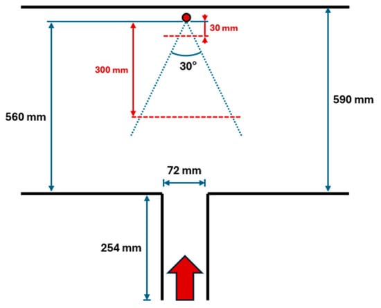
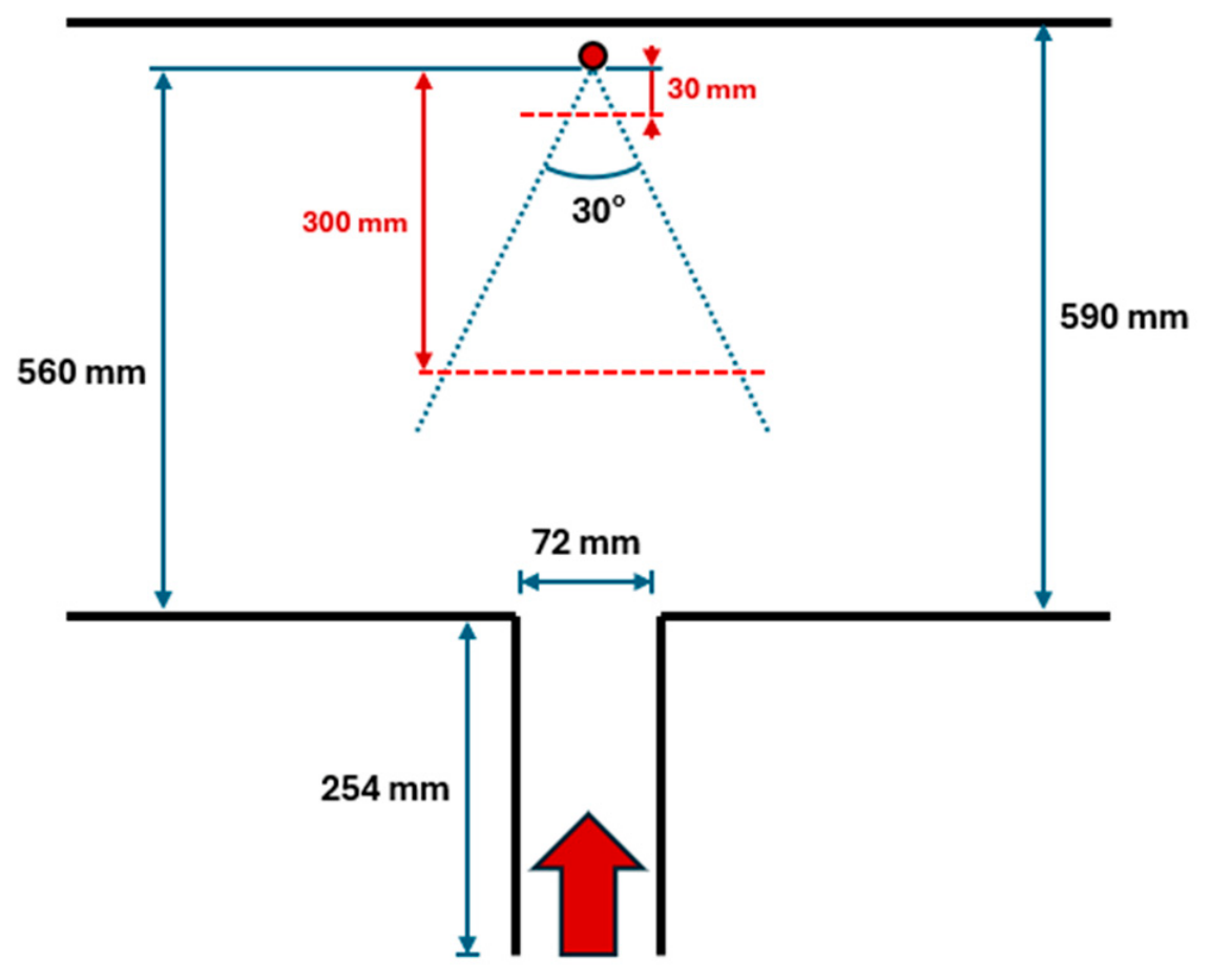
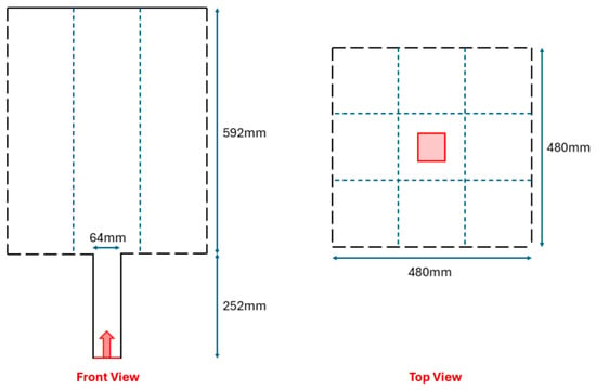
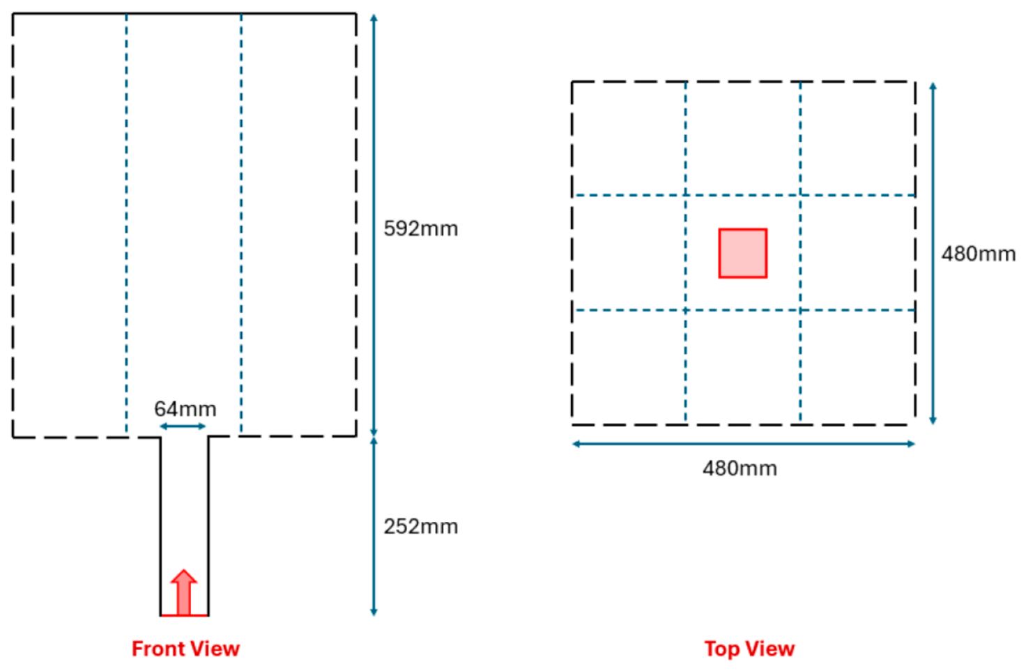
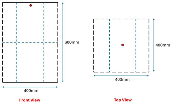
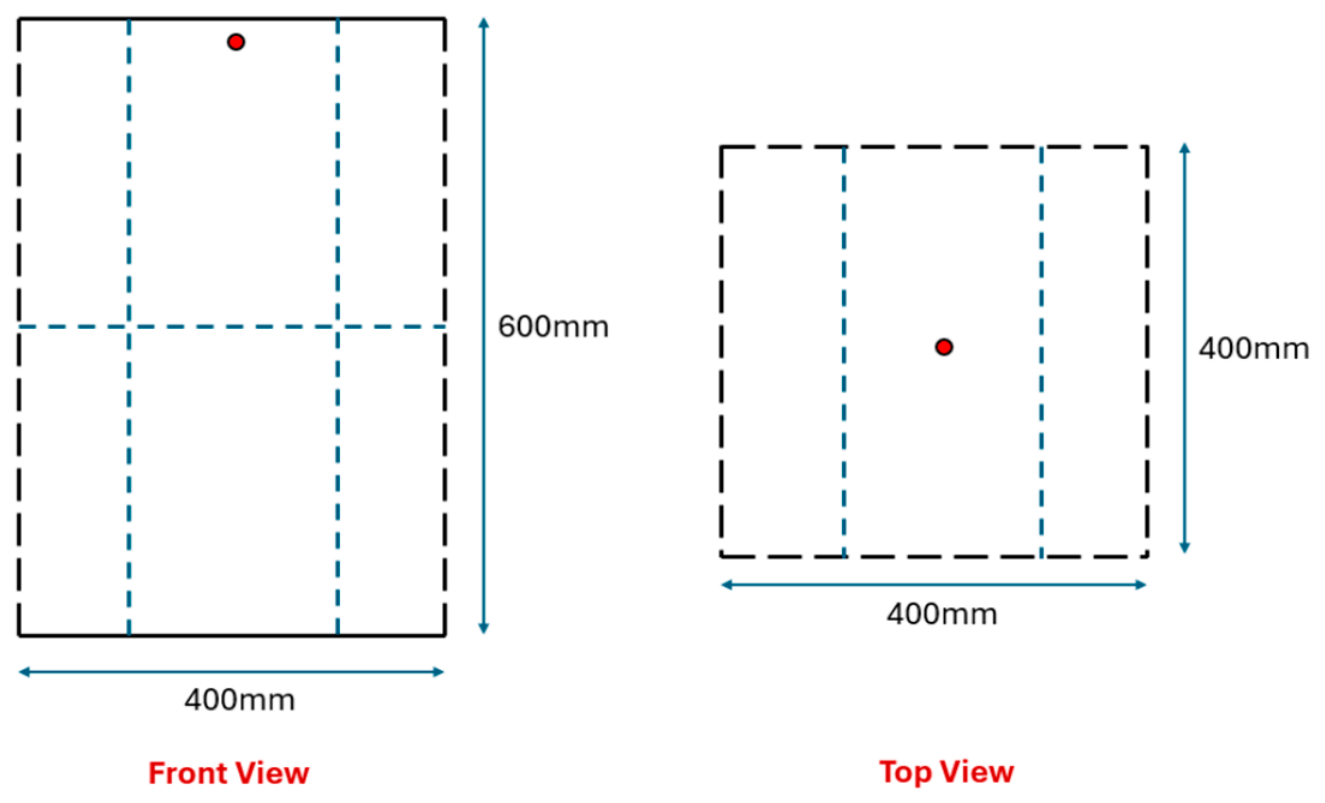
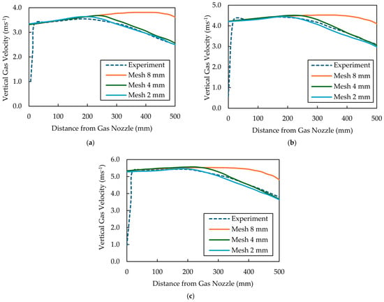
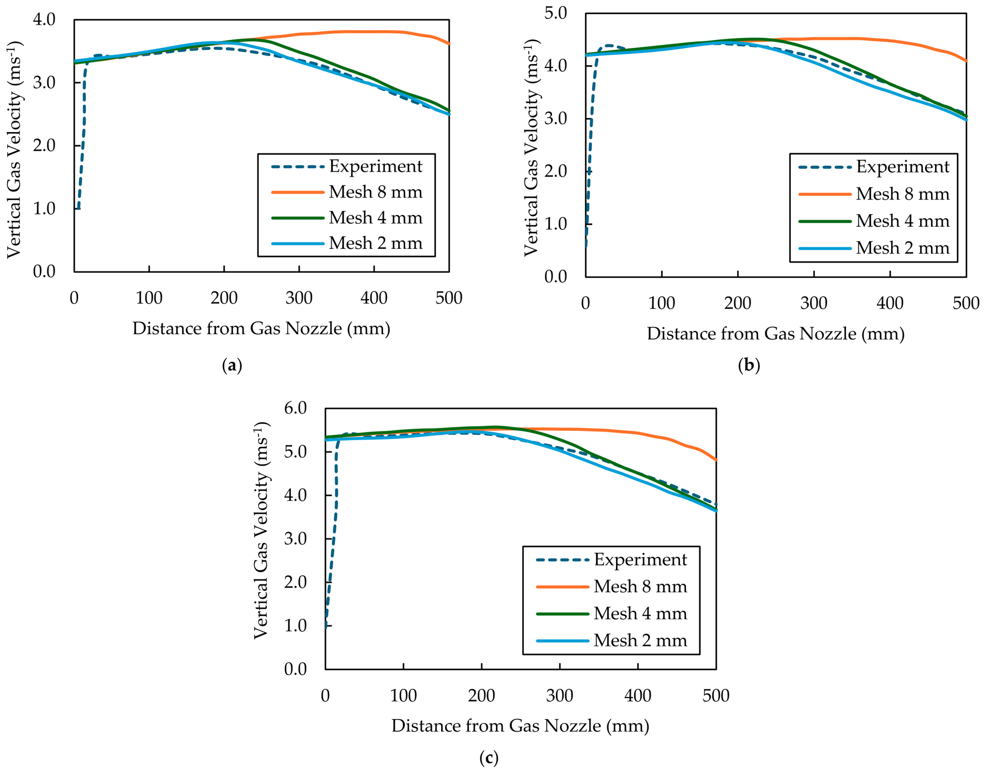
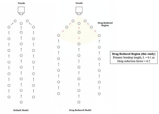
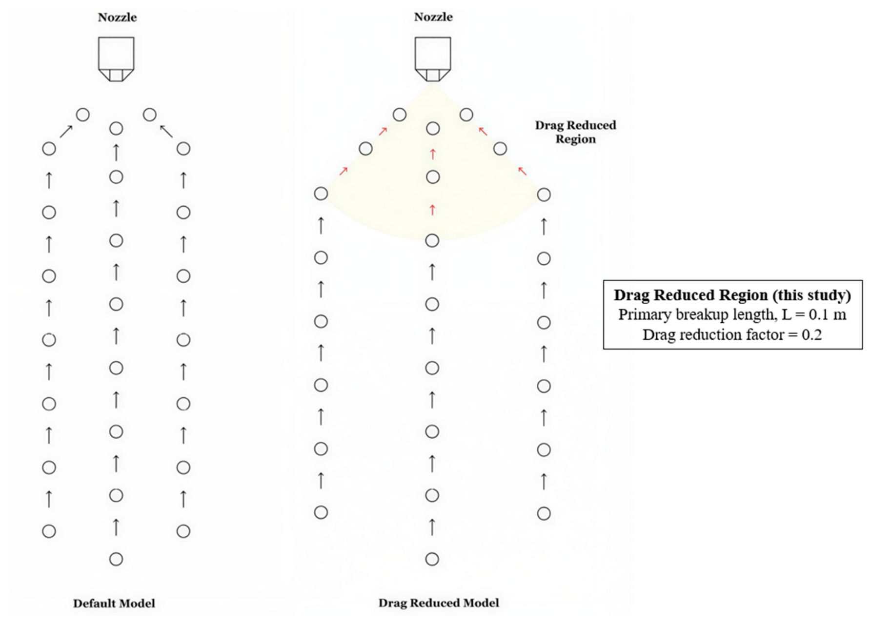
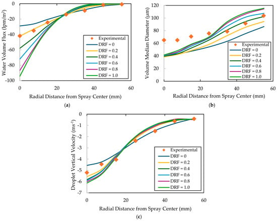
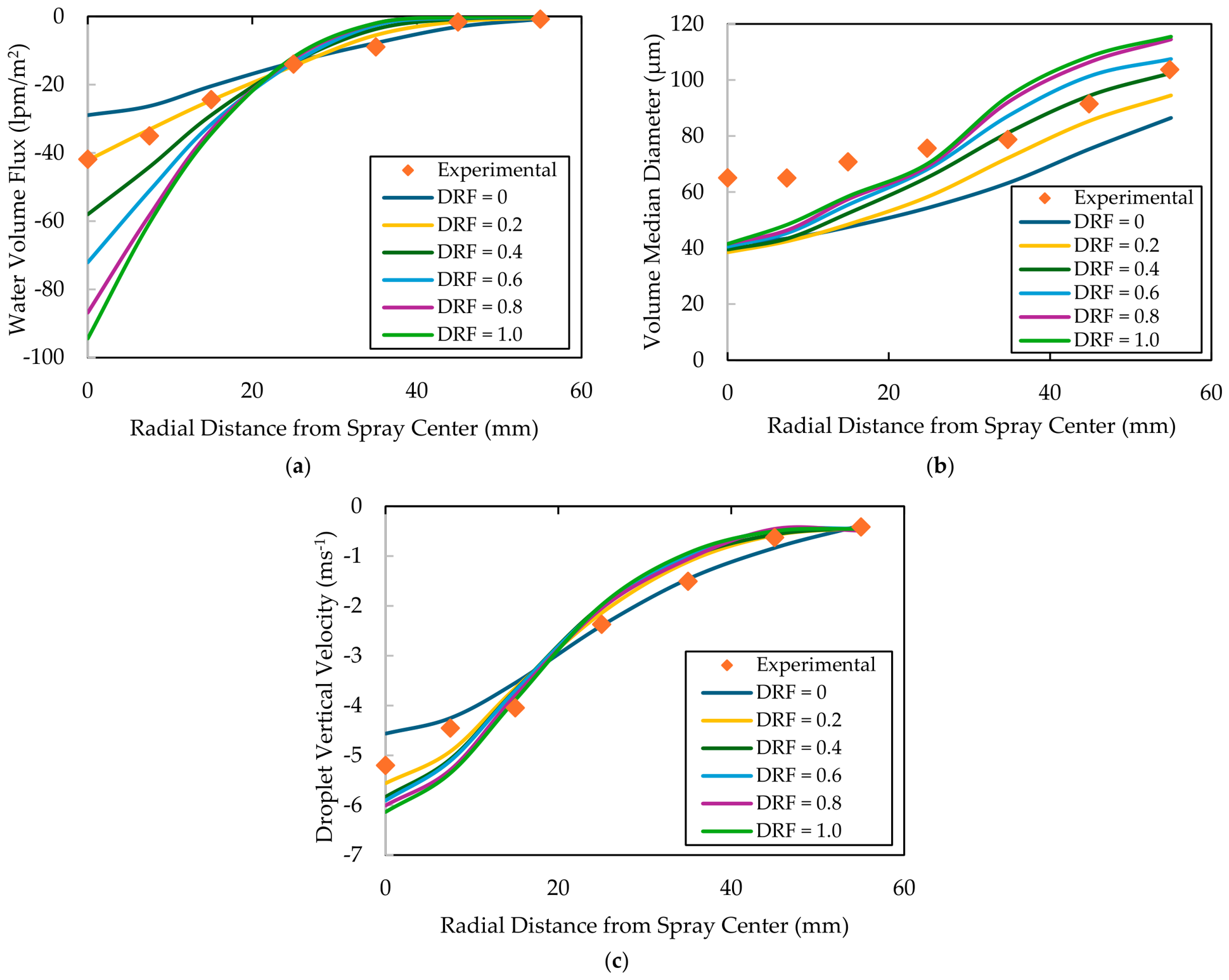
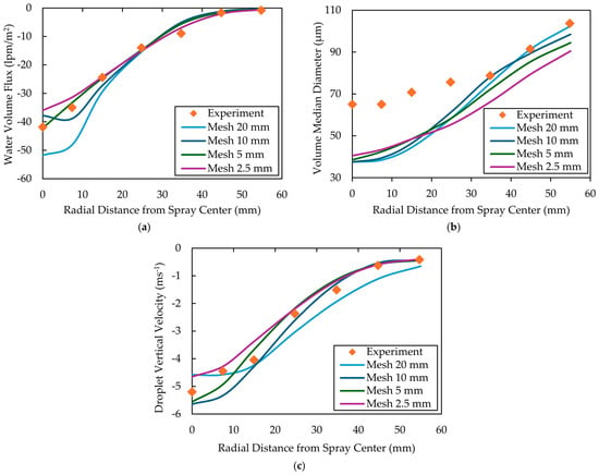
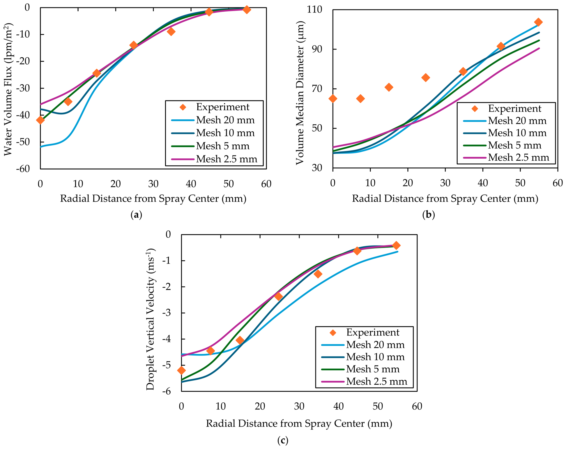
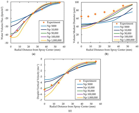
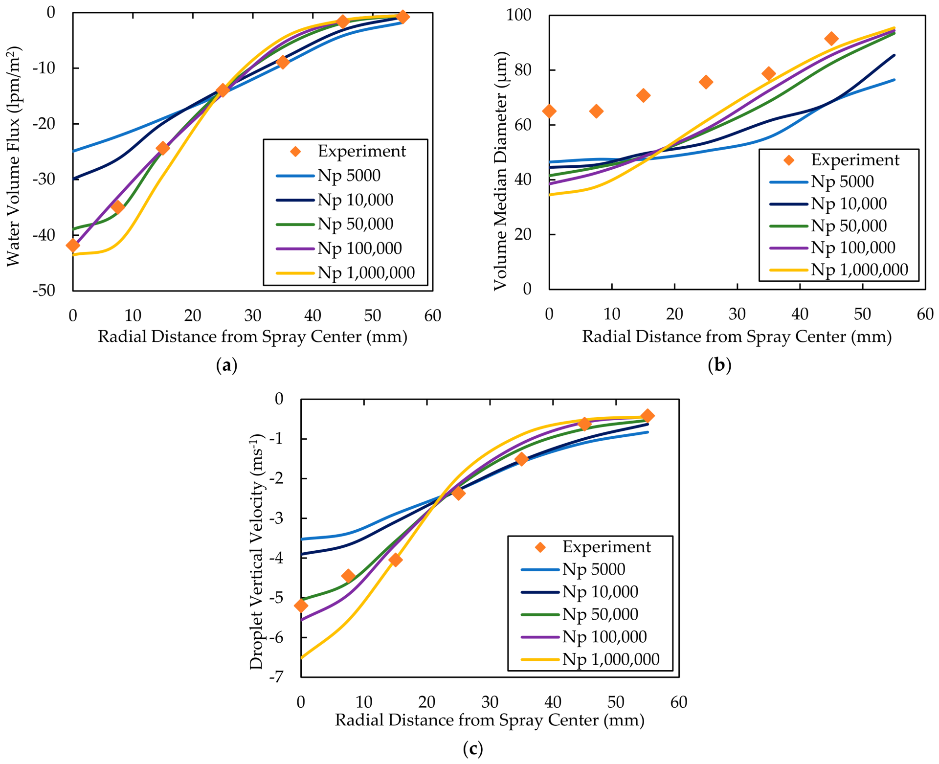
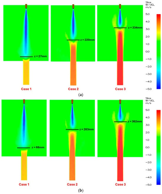

Disclaimer/Publisher’s Note: The statements, opinions and data contained in all publications are solely those of the individual author(s) and contributor(s) and not of MDPI and/or the editor(s). MDPI and/or the editor(s) disclaim responsibility for any injury to people or property resulting from any ideas, methods, instructions or products referred to in the content. |
© 2026 by the authors. Licensee MDPI, Basel, Switzerland. This article is an open access article distributed under the terms and conditions of the Creative Commons Attribution (CC BY) license.