


Abstract
The aerodynamic characterization of propeller-driven UAVs is often constrained by the unfeasibility of testing the complete airframe–propeller assembly in a wind tunnel, since geometric scaling prevents simultaneous similarity of both the airframe and the propeller. To address this limitation, this work presents an integrated experimental–numerical methodology that reconstructs the full-scale free-air aerodynamic behaviour of a tractor-propeller UAV combining wind-tunnel measurements of the scaled airframe (without the propeller) and the full-scale propeller. Computational fluid dynamics (CFD) is not used to predict the full-scale UAV directly; it is used to predict differences between matched configurations, while the absolute aerodynamic level remains anchored to experiments. Dedicated CFD simulations are carried out to isolate three distinct physical contributions: scale effects, wind-tunnel blockage, and propeller installation effects. In the developed methodology, numerical simulations complement the experimental data to obtain corrected full-scale aerodynamic coefficients and propulsive maps together with a longitudinal force-equilibrium model used to determine the longitudinal force-equilibrium operating point. The reconstruction shows that scale and wind-tunnel blockage effects primarily alter the airframe aerodynamic characteristics, with a minor influence on equilibrium incidence, while propeller installation produces a substantial thrust augmentation due to airframe-induced inflow modification. Accounting for these effects leads to an overprediction of the propeller rotational speed by approximately when installation effects are neglected, demonstrating that the installed performance cannot be obtained by a linear superposition of isolated airframe and isolated propeller data.
1. Introduction
Unmanned Aerial Vehicles (UAVs) have experienced rapid development over the last decade, driven by their increasing use in civil, commercial, and military applications [1,2,3]. Among the different available architectures [4,5], fixed-wing UAVs equipped with tractor propellers remain particularly attractive when endurance, payload capability, and aerodynamic efficiency are primary design requirements. As vehicle size and mission complexity increase [6,7], however, accurate aerodynamic characterization becomes increasingly challenging because airframe aerodynamics, propulsion performance, and their mutual interaction must be assessed under operating conditions that are representative of the full-scale vehicle.
Wind-tunnel testing remains one of the most reliable tools for aerodynamic characterization, but the direct extrapolation of model-scale measurements to full-scale free-air conditions is not straightforward. For clarity, the similarity requirements considered in the present work are distinguished from geometric similarity alone. Geometric similarity requires preservation of the nondimensional shape of the vehicle and its components. For the airframe, aerodynamic similarity additionally requires preservation of the nondimensional parameters governing the external flow, primarily the Reynolds number , where is the free-stream velocity, L a characteristic airframe length, the fluid density, and its dynamic viscosity. Indeed, it is well known that geometric scaling inevitably changes the Reynolds number and may therefore modify boundary-layer development, skin-friction contribution, pressure recovery, separation, and ultimately, the aerodynamic coefficients of the vehicle [8]. When compressibility effects are relevant, aerodynamic similarity also requires preservation of the Mach number , where a is the speed of sound. For the propeller, similarity requires preservation of the nondimensional operating and blade-flow conditions governing its aerodynamic performance—primarily the advance ratio (as defined in the following), the blade Reynolds number, and the blade-tip Mach number where relevant. Throughout the present work, these requirements are referred to as airframe aerodynamic similarity and propeller similarity, respectively. These similarity requirements also illustrate why a geometrically scaled complete vehicle cannot, in general, simultaneously reproduce the full-scale aerodynamic conditions of the airframe and propeller [9]. Let denote the geometric scale factor, such that and , with the subscript m indicating model-scale quantities and the subscript f indicating full-scale quantities. For the same working fluid, preservation of the airframe Reynolds number requires
Simultaneous preservation of the propeller advance ratio,
then requires
Consequently, decreasing the model scale requires both a higher tunnel velocity and an increased propeller rotational speed. For example, a 1:2 model would require twice the full-scale velocity and four times the full-scale rotational speed to simultaneously preserve airframe and propeller J. These requirements rapidly become incompatible with wind-tunnel velocity limits, allowable propeller rotational speeds, motor capabilities, and structural constraints. Moreover, simultaneous preservation of the blade Reynolds number and blade-tip Mach number introduces additional constraints that cannot generally be satisfied by matching and J alone. This incompatibility motivates the separate experimental characterization of the scaled airframe and full-scale isolated propeller adopted in the present work [10,11].
In addition, measurements performed in an open-jet test section are affected by facility-specific effects, including jet expansion and deflection, flow non-uniformity, nozzle and collector proximity, and aerodynamic interference generated by the model-support system [12,13,14]. Consequently, the aerodynamic coefficients measured on a scaled model cannot, in general, be directly interpreted as the full-scale free-air response of the aircraft.
The experimentally accessible airframe and propulsion measurements must therefore be connected to the target full-scale installed configuration through a reconstruction procedure that accounts for the physical differences between the tested and target conditions. In the present framework, this reconstruction is performed by retaining the experimental measurements as the absolute reference quantities and adding CFD-derived differential increments associated with each configuration change. Schematically,
where each is obtained from a matched pair of numerical configurations differing only in the physical effect to be corrected, namely, geometric scale, wind-tunnel confinement, or propeller installation. In fact, the term “configuration” refers here to a specific combination of geometric scale, flow domain condition (free air or virtual tunnel), and propeller state (isolated, absent, or installed). This reconstruction cannot be performed through a simple linear superposition of isolated airframe and propeller data. The propeller slipstream modifies the velocity field experienced by the fuselage and wing and alters the local and spanwise aerodynamic loading [15,16]. Conversely, the presence of the fuselage and lifting surfaces modifies the inflow experienced by the propeller and, therefore, changes its thrust, torque, and efficiency with respect to isolated operation [17,18]. Previous studies have shown that these aero-propulsive interactions can significantly affect lift, drag, pitching moment, and propulsive efficiency [19,20,21]. Therefore, even when accurate isolated measurements are available, the aerodynamic response of the complete vehicle remains unknown unless scale, facility, and installation effects are properly accounted for.
High-fidelity approaches, such as Large-Eddy Simulation (LES), can provide a detailed description of the complex flow structures and aerodynamic interactions characterizing bluff-body and complex configurations [22,23,24]. However, their computational cost remains prohibitive for the systematic exploration of the multiple geometries and operating conditions required by the present reconstruction framework. Reynolds-Averaged Navier–Stokes (RANS) approaches, combined with Moving Reference Frame (MRF) or moving-blade formulations, therefore represent a more practical alternative and are widely employed to predict the mean aerodynamic (e.g., drag modification) and propulsive performance of propeller-driven configurations [25,26,27,28,29]. Nevertheless, relying exclusively on absolute CFD predictions would transfer the full modelling uncertainty of the numerical solution to the reconstructed vehicle performance. Data-augmented approaches can further improve the predictive capability of lower-fidelity numerical models [30], but they generally require sufficiently extensive high-fidelity databases for training and validation, which are not always available for complex full-scale configurations. In the present study, the differential CFD database is generated using steady RANS simulations with the SST turbulence model, while propeller rotation is represented through a Moving Reference Frame (MRF) formulation. Transient moving-mesh simulations are employed only to assess the adequacy of the MRF approximation for the mean propulsive quantities relevant to the reconstruction.
In the present work, a different strategy is adopted: CFD is used in a differential rather than absolute sense. In the following, an “absolute” CFD prediction refers to the direct use of the numerical result as the estimate of the aerodynamic or propulsive quantity of interest for the target configuration, i.e., . In contrast, “differential” CFD is used here to estimate only the change in a quantity between two matched configurations A and B:
The corresponding target quantity is then reconstructed from the experimental reference as
The differential formulation does not eliminate numerical or model-form uncertainty, but it avoids relying exclusively on the absolute CFD prediction of the target configuration, which would transfer the full modelling uncertainty of the numerical solution to the reconstructed vehicle performance. In the present framework, this principle is applied sequentially to three main effects:
- (i)
- The Reynolds-number scale effect on the airframe;
- (ii)
- Wind-tunnel interference effects on both the airframe and the isolated propeller;
- (iii)
- The installation effect associated with the mutual aerodynamic interaction between the propeller and the airframe.
The corrected aerodynamic and propulsive models are finally coupled through a longitudinal force-equilibrium formulation to determine the longitudinal force-equilibrium operating point. The novelty of the proposed approach therefore does not reside in the use of CFD as a conventional correction tool for a single wind-tunnel experiment. Instead, as depicted earlier, it lies in the integration of experimentally accessible configurations that cannot simultaneously reproduce the full-scale aero-propulsive similarity of the complete vehicle. In particular, the identified research gap is addressed by decomposing the experimentally inaccessible complete-vehicle characterization into two experimentally accessible reference problems, as described in Section 3. The scaled rotorless-airframe campaign provides the experimental aerodynamic anchor, while the full-scale isolated-propeller campaign provides the corresponding propulsive anchor. They are connected to the target full-scale, free-air, installed configuration through a sequence of CFD-derived differential corrections. This provides a practical route to reconstruct the full-scale aero-propulsive behaviour when direct dynamically similar testing of the complete vehicle is not feasible. In this way, the proposed framework circumvents the conflicting similarity requirements of a geometrically scaled complete-vehicle experiment while retaining experimental measurements as the absolute reference levels of the reconstruction.
2. Problem Definition and Reconstruction Strategy
The aerodynamic reconstruction problem considered in this work concerns a fixed-wing UAV equipped with a single tractor propeller. The vehicle geometry is shown in Figure 1, while the main geometric parameters are summarized in Table 1. The wing planform area S and the mean aerodynamic chord c are adopted as reference quantities for the definition of the aerodynamic coefficients. Unless otherwise stated, all aerodynamic coefficients reported throughout the paper refer to these reference quantities.
Figure 1.
Isometric sketch of the analysed fixed-wing UAV.
Table 1.
Wing geometry and reference aerodynamic parameters.
The wind-tunnel airframe is a geometrically scaled representation of the full-scale UAV, with a linear scale factor
where the subscripts SC and FS denote the scaled and full-scale configurations, respectively. Throughout the manuscript, the labels VT and FA are additionally used to identify virtual-tunnel and free-air conditions.
The aerodynamic forces acting on the airframe are expressed in terms of the conventional lift and drag coefficients, defined as
where L and D denote the aerodynamic lift and drag forces, respectively, is the air density, and is the freestream velocity.
The propulsion system consists of a MEJZLIK tractor propeller. Propeller performance is described in terms of the advance ratio J:
where n is the rotational speed expressed in revolutions per second, and is the propeller diameter. For convenience, hereafter, the propeller rotational speed is also reported in revolutions per minute as .
The corresponding thrust and torque coefficients are defined as
where T and Q denote propeller thrust and torque, respectively. The power coefficient and propulsive efficiency are consequently given by
The aerodynamic and propulsive quantities defined above cannot all be measured directly for the target full-scale installed configuration. The available wind-tunnel experiments instead provide the aerodynamic characteristics of a geometrically scaled rotorless airframe and the performance of the isolated full-scale propeller. The objective is therefore to reconstruct the aerodynamic and propulsive characteristics of the complete full-scale UAV operating in free air by combining these experimentally accessible quantities with differential corrections obtained from CFD.
2.1. Differential-Reconstruction Procedure
Two numerical-domain conditions are used throughout the reconstruction. The virtual-tunnel (VT) configuration reproduces the experimental wind-tunnel environment, including the test-section geometry and associated confinement effects, and therefore constitutes the numerical counterpart of the corresponding wind-tunnel experiment. In contrast, the free-air (FA) configuration places the same aerodynamic or propulsive system in an extended numerical domain designed to approximate unconfined external-flow conditions. The installed (INST) configuration, instead, includes the complete airframe–propeller geometry. Throughout the present work, SC denotes the scaled model and FS denotes the full-scale configuration. The configurations involved in the differential reconstruction are summarized in Table 2. The notation introduced here is used consistently throughout the remainder of the paper.
Table 2.
Summary of the configurations involved in the differential reconstruction framework.
The general reconstruction principle adopted in the present work can be expressed as
where denotes an experimentally measured coefficient, is the corresponding quantity in the target configuration, and represents the i-th correction required to transfer the experimental quantity to the target condition.
For the present problem, the complete correction hierarchy may be written schematically as
where accounts for Reynolds-number scaling as determined from matched SC–FS comparisons, represents wind-tunnel interference and blockage effects obtained through matched VT–FA comparisons, and accounts for the aerodynamic interaction between the propeller and the airframe evaluated via matched FA–INST comparisons. Not all terms in Equation (7) apply to every aerodynamic quantity; rather, the specific correction chain depends on whether the airframe or the propulsion system is considered.
For the rotorless airframe, the reconstruction from the scaled wind-tunnel configuration to full-scale free-air conditions is written as
whereas the isolated-propeller measurements are transferred from wind-tunnel to free-air conditions according to
The final step accounts for the aerodynamic interaction between the propeller and the airframe. The installed-propeller coefficients are reconstructed as
Equations (6)–(10) provide the general structure of the reconstruction framework. Their central feature is that CFD is not used to determine the absolute aerodynamic and propulsive coefficients of the target vehicle. Instead, each correction term is obtained from the difference between two matched numerical configurations:
where configurations A and B are selected so as to isolate the physical contribution of interest. The experimental measurements therefore remain the reference aerodynamic and propulsive levels, while CFD provides only the differential information required to transfer them toward the target configuration.
This differential formulation is particularly useful when the absolute numerical prediction may be affected by modelling uncertainties that are partially common to the two matched CFD configurations. The methodology relies on the numerical prediction of the change produced by a controlled modification of the configuration, rather than on the absolute CFD solution alone.
2.2. Closure of the Differential Reconstruction
An important property of the proposed formulation can be illustrated for the airframe reconstruction. The scale correction is obtained by comparing the full-scale and scaled airframes under free-air conditions:
whereas the wind-tunnel correction is determined by comparing the scaled airframe in free air and in the virtual wind tunnel:
Equation (15) highlights a useful closure property of the differential reconstruction. The discrepancy between the reconstructed full-scale coefficient and the corresponding full-scale CFD solution is directly related to the discrepancy between the wind-tunnel measurement and its numerical counterpart in the virtual wind tunnel. Consequently, agreement between the experiment and the matched virtual-tunnel simulation provides a direct assessment of the consistency of the reconstruction chain.
An analogous relation applies to the isolated-propeller reconstruction. Defining the wind-tunnel correction as
Equation (9) yields
The same closure principle therefore applies independently to the aerodynamic and propulsive branches of the reconstruction framework.
The installation correction represents the final step of the procedure and differs conceptually from the scale and wind-tunnel corrections because it introduces the mutual aerodynamic interaction between the airframe and the propeller. It is determined by comparing the installed and isolated full-scale propeller configurations under otherwise matched operating conditions:
The resulting corrected airframe and installed-propeller models provide the aerodynamic and propulsive quantities required to reconstruct the operating condition of the complete vehicle.
2.3. Target Operating Condition
The final objective of the reconstruction is to determine the cruise operating condition of the complete full-scale UAV. The present analysis is restricted to longitudinal translational force equilibrium. A complete aerodynamic trim, which would additionally require pitching-moment equilibrium and the explicit modelling of the corresponding control surfaces, is outside the scope of the present work.
In particular, the propeller slipstream may modify the aerodynamic loading of the wing and tail surfaces, thereby introducing additional pitching-moment contributions with respect to the rotorless-airframe condition. A complete trimmed-flight reconstruction would therefore require the corresponding installation-induced pitching-moment correction to be included together with the control-surface deflections required to satisfy moment equilibrium. Consequently, the values of and determined in the present analysis should be interpreted as a longitudinal translational force-equilibrium operating point rather than as a fully trimmed cruise condition. Extension of the differential reconstruction framework to pitching-moment and control-surface effects represents a natural development of the present methodology.
The reconstructed airframe and installed-propeller models are therefore subsequently coupled through the longitudinal force-equilibrium equations to determine the equilibrium angle of attack and propeller rotational speed . This final step provides a direct means of assessing how the different correction mechanisms (scale effects, wind-tunnel interference, and propeller installation) propagate from the individual aerodynamic and propulsive coefficients to the predicted operating condition of the complete vehicle.
The experimental campaigns used to provide the reference airframe and propeller data are described in the following section, while the CFD configurations employed to evaluate the differential corrections introduced above are presented in Section 4.
3. Experimental Investigation
Two independent wind-tunnel campaigns were conducted to provide the experimental reference data required by the differential reconstruction framework introduced in Section 2. The first campaign (E1) characterized a geometrically scaled rotorless UAV and provided the baseline aerodynamic coefficients of the airframe. The second campaign (E2) characterized the isolated full-scale propeller over the range of advance ratios and disk-incidence angles relevant to the target operating conditions. Details are summarized in Table 3.
Table 3.
Summary of the experimental campaigns used as reference conditions for the differential reconstruction framework.
The different scales adopted in the two experimental campaigns are intentional. The airframe was tested as a 1:14 geometrically scaled model to obtain an experimentally feasible configuration within the available wind-tunnel facility; the resulting Reynolds-number mismatch with respect to the full-scale vehicle is subsequently accounted for through the differential CFD reconstruction. Conversely, the propulsion system could be tested directly at full scale. This choice avoids introducing additional propeller-scaling effects associated with blade Reynolds number and rotational-speed requirements, and it allows the isolated propeller to be characterized over the advance-ratio range relevant to the target vehicle.
These measurements constitute the absolute reference levels of the reconstruction procedure. The corresponding CFD simulations introduced in Section 4 were therefore designed to reproduce the experimental configurations as closely as possible before extracting the differential corrections required to transfer the measurements toward the target full-scale free-air configuration.
3.1. Wind-Tunnel Facility and Measurement System
Both experimental campaigns were carried out in the open-jet wind tunnel of the Department of Civil and Industrial Engineering at the University of Pisa. The facility has a circular open test section with a diameter of and a length of . The maximum freestream velocity is approximately , while the freestream turbulence intensity in the test section is approximately ([31]).
The open-jet configuration, together with the finite dimensions of the test section and the presence of the model-support system, may introduce aerodynamic interference with respect to the corresponding free-air configuration. These effects include jet expansion and deflection, streamwise pressure gradients, nozzle and collector proximity, and aerodynamic interaction between the model and its support system. Rather than applying conventional analytical corrections, the complete wind-tunnel flow path and the relevant support geometries were explicitly reproduced in the virtual-tunnel CFD configurations described in Section 4.
The operating conditions of the two experimental campaigns were selected according to their different roles in the reconstruction framework, rather than to simultaneously match all full-scale nondimensional parameters. In E1, the 1:14 rotorless-airframe model was tested at , resulting in a Reynolds number lower than that of the target full-scale vehicle; this deliberate mismatch was subsequently accounted for through the CFD-derived scale correction, as detailed below. In E2, the full-scale propeller was tested directly, and the combinations of freestream velocity and rotational speed were selected to span the advance-ratio range relevant to the target operating conditions. The investigated disk-incidence angles similarly cover the oblique-inflow conditions relevant to the UAV operating envelope.
The two experimental campaigns employed dedicated measurement systems because of the substantially different force and torque ranges associated with the scaled airframe and the full-scale propeller. The corresponding instrumentation, calibration procedures, acquisition parameters, and measurement uncertainties are described in the following sections.
3.2. Scaled Rotorless-Airframe Experiment
The first experimental campaign (E1) was performed on a 1:14 geometrically scaled model of the UAV airframe. The propeller was not installed during these measurements, so that the resulting aerodynamic coefficients represent the rotorless-airframe contribution independently of propulsion effects.
The model was tested at a freestream velocity of , over the investigated range of incidence angles. Lift and drag were measured using the wind-tunnel force-balance system and converted into the aerodynamic coefficients defined in Section 2. The Reynolds number based on the mean aerodynamic chord is defined as , where is the mean aerodynamic chord of the tested configuration. Owing to the 1:14 geometric scaling, the Reynolds number of the wind-tunnel model is substantially lower than that corresponding to the target full-scale vehicle. This mismatch constitutes the Reynolds-number scale effect subsequently quantified through the differential CFD procedure.
The model was mounted in the open test section using the support assembly shown in Figure 2. Since the experimental configuration differs from the corresponding free-air condition not only because of Reynolds-number scaling but also because of wind-tunnel and support interference, the reconstruction of the full-scale rotorless-airframe coefficients requires the two differential contributions introduced in Section 2.
Figure 2.
Experimental configuration of the 1:14 scaled rotorless UAV in the University of Pisa wind tunnel. Model support (1), balance (2), rear sting (3), and model (4).
The measured lift and drag coefficients therefore provide the experimental anchor of the airframe branch of the reconstruction, rather than a direct estimate of the full-scale free-air aerodynamic characteristics.
3.3. Full-Scale Isolated-Propeller Experiment
The second experimental campaign (E2) characterized the MEJZLIK (Brno, Czech Republic) propeller independently of the airframe. Unlike the airframe experiment, no geometric scaling of the propulsion system was introduced, and the full-scale propeller was tested directly in the wind tunnel, as depicted in Figure 3.
Figure 3.
Experimental configuration of the MEJZLIK 24 × 12 propeller in the University of Pisa wind tunnel.
The propeller was characterized over a range of rotational speeds and freestream velocities, allowing its performance to be expressed in terms of the advance ratio, as defined in Section 2. Tests were also performed at different disk-incidence angles () in order to characterize the variation in propeller performance under oblique inflow conditions representative of the UAV operating envelope.
Thrust and torque were measured independently and converted into the nondimensional coefficients and . The resulting experimental database therefore provides
Figure 4 shows the measured thrust-coefficient map as a function of advance ratio and disk incidence. The measurements indicate a systematic dependence of propeller thrust on both variables, which must be retained when the propulsive model is subsequently coupled with the airframe aerodynamic model.
Figure 4.
Experimental map of the thrust coefficient as a function of the incidence angle and the advance ratio J.
Since the longitudinal force-equilibrium analysis developed in Section 6 requires the continuous evaluation of propeller thrust as a function of both rotational speed and incidence, the discrete experimental database was represented through a compact response-surface formulation. The correlation was obtained by ordinary least-squares regression over the complete experimental dataset, with equal weighting assigned to all measurement points. The coefficients were determined by minimizing the sum of the squared residuals between the measured and fitted thrust coefficients:
where the fitted coefficients are , , , and .
The resulting fit provides a coefficient of determination and a root-mean-square error , indicating that the adopted formulation provides an adequate representation of the measured thrust coefficient over the investigated operating range.
The purpose of Equation (21) is not to provide a general propeller-performance model outside the experimentally investigated domain but to interpolate the measured thrust data within the range required by the subsequent reconstruction and force-equilibrium analysis. Although both thrust and torque were measured and are considered when assessing wind-tunnel and installation effects, only the thrust response surface is required to determine the longitudinal force-equilibrium operating point.
As for the airframe, the wind-tunnel measurements of the isolated propeller do not directly represent its free-air performance because of wind-tunnel interference. They therefore constitute the experimental anchor of the propulsion branch of the reconstruction,
before the additional installation correction is introduced to account for the mutual aerodynamic interaction between the propeller and the airframe.
3.4. Experimental Errors and Repeatability
Aerodynamic loads for both experimental campaigns were measured using in-house-developed six-component strain-gauge balances specifically selected and calibrated for the corresponding load ranges. For E1, the balance was used to determine the aerodynamic force components required to obtain airframe lift and drag, whereas for E2 a dedicated balance was employed to measure propeller thrust and torque. The balance was calibrated prior to the tests by applying known loads over the relevant measurement ranges. The calibration procedure utilized a comprehensive set of load configurations and a least-squares regression to effectively resolve cross-coupling effects between the components. The resulting calibration residuals were used to quantify the systematic measurement uncertainty. Post-calibration verification demonstrated maximum absolute residuals in the order of approximately for the force components, ensuring a global relative error strictly below . To further ensure measurement fidelity, linear corrections were applied to account for the thermal drift of the strain-gauge bridges, utilizing zero-load readings recorded immediately before and after each wind-tunnel run. Finally, to bound the statistical random error below while preventing excessive thermal accumulation in the sensors, data acquisition was standardized at a sampling frequency of for approximately 16 s ( samples) per measurement point. Experimental uncertainty was evaluated by accounting separately for measurement repeatability and balance calibration. For each operating condition, 10 repeated measurements were acquired. The repeatability contribution was evaluated from the statistical dispersion of the repeated measurements. The calibration contribution was determined from the residual differences between the known loads applied during calibration of the in-house force/torque balances and the corresponding loads reconstructed from the calibration model. Assuming the two contributions to be independent, the combined standard uncertainty was evaluated as . The resulting force and torque uncertainties were propagated to the corresponding nondimensional coefficients , , , and . The errors associated with repeatability were evaluated through the Standard Error of the Mean (SEM):
where denotes the i-th sample of the measured signal and is the sample mean. The SEM was propagated through the tare subtraction assuming independence between the two measurements:
The systematic error was obtained from the balance calibration, where the residuals between applied and reconstructed loads provide an equivalent one-standard-deviation error for each balance-frame component. This error was mapped to the wind-axis lift and drag components using the same transformations applied to the mean forces. The total error for each aerodynamic force was obtained by combining the statistical and calibration terms in quadrature,
with .
The resulting errors were propagated to the nondimensional aerodynamic and propulsive coefficients and subsequently retained in the reconstruction procedure. Their effect on the final equilibrium angle of attack and propeller rotational speed is quantified through the uncertainty-propagation analysis presented in Section 6.
4. Numerical Methodology
The numerical simulations employed in the differential reconstruction framework were performed using a consistent CFD methodology across all configurations introduced in Section 2. This section describes the governing numerical approach, computational domains, mesh-generation strategy, convergence criteria, and propeller modelling adopted throughout the study. The computational configurations and their role within the reconstruction framework are summarized in Table 4.
Table 4.
Summary of the computational configurations employed in the differential reconstruction framework.
The numerical methodology is assessed through three complementary procedures: grid-refinement analysis of the integral quantities entering the reconstruction (Section 4.1.1), comparison of the steady MRF propeller model with transient moving-mesh simulations (Section 4.1.2), and direct comparison with the experimentally available configurations (Section 5.3).
4.1. Simulation Set-Up
All computational configurations were simulated within a Reynolds-Averaged Navier–Stokes (RANS) framework using the SST k– turbulence model. The model was selected because of its established performance in external aerodynamic flows involving adverse pressure gradients and flow separation, which are relevant to the present UAV configuration. For the virtual wind-tunnel simulations, the freestream turbulence intensity was prescribed consistently with the experimentally measured value of approximately 0.9%.
Although the boundary layer is expected to be predominantly turbulent over most of the airframe, the substantial Reynolds-number difference between the scaled and full-scale configurations modifies the boundary-layer development, skin-friction contribution, pressure recovery, and separation behaviour predicted within the adopted RANS framework. The resulting configuration-to-configuration variation is therefore incorporated into the CFD-derived scale correction. These effects are therefore retained in the numerical solution and constitute part of the scale correction quantified in Section 5.1.
A second-order spatial discretization was adopted for all governing equations. Pressure and velocity were coupled through a coupled solution algorithm. Air density was treated as constant, consistent with the low-Mach-number operating conditions considered in the present study.
All steady computations were continued until both the equation residuals and the integral aerodynamic quantities reached stationary values. In particular, convergence of the aerodynamic solution was assessed by monitoring the integrated force and moment coefficients, and the simulations were considered converged when their residual variations were accompanied by variations in the integral aerodynamic loads below 1%.
Grid generation followed a consistent parametric strategy across the different configurations. Polyhedral cells were employed in the outer flow domain, while prismatic layers were generated on all solid surfaces to resolve the near-wall velocity gradients. Local volumetric refinements were introduced around the airframe, propeller blades, and wake regions. The height of the first prism layer and the total boundary-layer thickness were selected to obtain , placing the first computational cell within the logarithmic region consistently with the adopted wall-function treatment. The same nondimensional near-wall strategy was retained for all geometrically corresponding configurations, so that the differential corrections were evaluated between solutions obtained with a consistent turbulence and wall-treatment formulation. This modelling strategy was selected to provide a uniform and computationally affordable representation of the mean integral aerodynamic quantities over the complete multi-configuration CFD campaign. The SST formulation is used to represent the adverse-pressure-gradient and moderate-separation effects encountered within the operating range relevant to the reconstruction. However, the adopted wall-function treatment is not intended to provide a wall-resolved description of skin friction or strongly separated post-stall flow. In addition, laminar-to-turbulent transition is not explicitly modelled in the present simulations. The predicted Reynolds-number scale correction should therefore be interpreted as the change in aerodynamic response obtained within a consistently applied fully turbulent RANS framework. Possible scale effects associated specifically with variations in transition location are not independently resolved and represent a limitation of the present approach.
The computational domains were designed according to the physical configuration to be reproduced. For the virtual wind-tunnel simulations, the computational model explicitly reproduced the relevant wind-tunnel flow path, including the nozzle, open test section, diffuser, downstream region, and model-support assembly. The resulting SC–VT configuration is shown in Figure 5. Inclusion of the support geometry was particularly important because its aerodynamic contribution is inherently contained in the experimental measurements and must therefore also be represented in their numerical counterpart.
Figure 5.
Computational representation of the scaled rotorless airframe in the virtual wind tunnel (SC–VT configuration), including the wind-tunnel flow path and model-support assembly.
At the wind-tunnel inlet, the mass flow rate was prescribed to reproduce a jet velocity of m/s in the test section. The downstream boundary was treated as a pressure outlet. The diffuser and all solid components of the model and support system were treated as no-slip surfaces, whereas the appropriate tunnel boundaries were treated according to the experimental flow-path representation.
The free-air simulations (SC–FA, FS–FA, PROP–FA, and PROP–INST) were performed in domains sufficiently large to minimize aerodynamic interference from the outer boundaries. For the airframe configurations, the computational domain extended approximately upstream of the aircraft nose and downstream, with lateral and vertical extents of approximately , where is the mean aerodynamic chord defined in Section 2. The same nondimensional domain dimensions were retained for the scaled configuration.
For the isolated-propeller simulations, a cubic computational domain with a characteristic dimension of approximately was employed, where is the propeller diameter. Dedicated cylindrical refinement regions were introduced downstream of the propeller to resolve the development of the slipstream and blade-tip vortices. The upstream boundary was prescribed as a velocity inlet, the downstream boundary as a pressure outlet, and the lateral outer boundaries were treated as slip surfaces. No-slip conditions were imposed on all solid surfaces.
The complete installed configuration (PROP–INST) retained the free-air domain philosophy while simultaneously resolving the airframe, propeller, and the propeller-generated slipstream. This configuration represents the numerical target required to isolate the propeller–airframe installation effect discussed in Section 5.4.
4.1.1. Grid-Sensitivity Analysis
A grid-sensitivity analysis was performed using three progressively refined mesh levels for both the airframe and propeller configurations. The full-scale free-air configurations (FS–FA and PROP–FA) were selected for this analysis to avoid additional facility-related effects and to represent the corresponding free-air configurations used in the reconstruction procedure. The airframe grids contained approximately 12.5, 18.0, and 33.0 million cells for the coarse, medium, and fine levels, respectively, while the corresponding propeller grids contained approximately 2.5, 4.0, and 6.0 million cells. Grid sensitivity was assessed by monitoring the integral quantities directly employed in the reconstruction, namely, and for the airframe, and and for the propeller. The fine-grid solution was adopted as the highest-resolution reference, and the percentage differences reported in Table 5 were evaluated relative to this solution.
Table 5.
Grid-sensitivity analysis for the full-scale rotorless airframe (FS–FA) and isolated propeller (PROP–FA). Percentage differences are evaluated with respect to the corresponding fine-grid solution, used as the highest-resolution reference.
The differences decreased with progressive mesh refinement. The medium-to-fine differences were approximately 0.8% for and 1.7% for for the airframe, and 1.2% for and 1.9% for for the propeller. Since a formal Richardson extrapolation or Grid Convergence Index (GCI) analysis was not performed, the fine-grid solution is used as the highest-resolution reference rather than as a formally grid-independent solution. Since the medium-to-fine differences remained below 2% for all four monitored coefficients, the medium mesh was retained for the systematic multi-configuration CFD campaign. The same relative meshing strategy was maintained across the matched configurations used to evaluate each differential correction. The resulting meshes contained approximately 18.0 million cells for the FS–FA configuration and 4.0 million cells for PROP–FA. The virtual-tunnel configurations required approximately 22.0 million cells for SC-VT and 10.0 million cells for PROP–VT, owing to the additional refinement around the wind-tunnel geometry and support system. The complete PROP–INST configuration contained approximately 21.0 million cells.
4.1.2. Propeller Modelling
Propeller rotation was modelled using a steady Moving Reference Frame (MRF) approach throughout the differential reconstruction campaign. In the MRF formulation, the computational mesh remains stationary while the governing equations are expressed in a rotating reference frame within a cylindrical region surrounding the propeller. This approach reproduces the mean effect of blade rotation and propeller-induced flow while avoiding the substantially greater computational cost associated with a fully transient moving mesh with sliding interface simulation. The rotating region was defined as a cylindrical domain surrounding the propeller, with a diameter of approximately and an axial extent of approximately . These dimensions were selected following a preliminary sensitivity assessment to provide sufficient separation between the blade surfaces and the rotating–stationary interface without unnecessarily increasing the computational cost.
The MRF approach cannot resolve blade-passage effects, periodic force fluctuations, or other intrinsically unsteady features of the propeller wake. Since the proposed reconstruction framework is based on mean aerodynamic and propulsive quantities, the adequacy of the MRF approximation was assessed against transient blade-resolved moving-mesh simulations. In addition to the reference installed operating condition at and m/s, two additional conditions were selected to span the range of advance ratio and propeller incidence. As shown in Table 6, we selected one additional configuration with low J and another with a high angle of attack to verify the modelling assumptions across the full range of operating conditions relevant to the reconstruction. The MRF and moving-mesh (MM) simulations were performed using the same computational grid, so that the observed differences could be primarily associated with the rotating-flow modelling approach.
Table 6.
Comparison between steady MRF and time-averaged MM predictions at three representative installed operating conditions. Percentage differences are evaluated with respect to the corresponding time-averaged moving-mesh values.
The moving-mesh thrust coefficients were time-averaged over 5 complete propeller revolutions after the initial transient had decayed. As summarized in Table 6, the differences in the time-averaged thrust coefficient between the MRF and moving-mesh solutions were 0.09%, 1.17%, and 2.99% for the three investigated operating conditions, respectively, with a maximum difference of approximately 3%. The comparison is restricted to the mean propulsive response and does not constitute an assessment of turbulence-model accuracy. Nonetheless, the small differences observed (below 3%) justify the use of the steady-MRF formulation for the present reconstruction, as it provides accurate mean propulsive coefficients at a substantially lower computational cost than the moving-mesh approach.
5. CFD-Informed Differential Reconstruction
The experimental campaigns described in Section 3 provide the absolute aerodynamic and propulsive reference levels of the reconstruction framework. The CFD simulations described in Section 4.1 are now used to determine the differential corrections required to transfer these measurements from the experimentally accessible configurations to the target full-scale free-air vehicle.
Consistent with the formulation introduced in Section 2, the numerical simulations are not used to replace the experimental database with absolute CFD predictions. Instead, pairs of matched computational configurations are compared to isolate the effects of Reynolds-number scaling, wind-tunnel interference, and propeller installation. The resulting increments are subsequently applied to the corresponding experimental measurements.
The reconstruction is organized into two main branches: The first transfers the scaled rotorless-airframe measurements to the full-scale free-air condition through scale and wind-tunnel corrections. The second transfers the isolated-propeller measurements to free-air conditions and subsequently introduces the propeller–airframe installation effect. The two reconstructed models are finally coupled in Section 6 to determine the longitudinal force-equilibrium operating point.
5.1. Airframe Reconstruction
For the rotorless airframe, three CFD configurations listed in Table 4 are used: the full-scale airframe in free air (FS–FA), the scaled airframe in free air (SC–FA), and the scaled airframe in the virtual wind tunnel (SC–VT). At a given incidence , the corresponding aerodynamic coefficients are denoted by , , and , where .
The scale increment quantifies the difference between the full-scale and scaled free-air responses:
Figure 6 presents the scale-induced lift and drag increments, calculated within the interval of linearity of the – curve. The lift increment increases approximately linearly with incidence within the attached-flow regime. At low angles, the increment remains small, indicating limited sensitivity of the scaled configuration to Reynolds-number effects under mild aerodynamic loading. As increases, grows steadily and follows a near-linear trend over the pre-stall interval. The drag increment correlates negatively with over the same interval. The magnitude of the increment increases gradually with , and the fitted trend captures the dominant behaviour in the attached-flow regime.
Figure 6.
Scale-induced aerodynamic increments computed via CFD. (Left): Lift increment as a function of incidence. (Right): Drag increment as a function of . Linear regressions highlight the dominant trends.
The scale increments are approximated using the linear relations
The fitted coefficients are , , , and .
The blockage increment is defined as the difference between the scaled free-air SC–FA and scaled virtual-tunnel SC–VT responses:
This term quantifies the net effect of wind-tunnel blockage, jet non-uniformity, and support interference, consistent with the principal open-jet and support-interference mechanisms described in [12,13]. Figure 7 presents the blockage-induced lift and drag increments. The lift increment decreases approximately linearly with incidence over the attached-flow interval, with the corresponding linear regression yielding . The drag increment exhibits a positive correlation with the corresponding lift modification, albeit with a larger relative scatter, as indicated by . The lower coefficient of determination obtained for the drag correction should be interpreted in relation to the comparatively small absolute magnitude of . Since this quantity is obtained as the difference between the drag coefficients predicted for two closely matched CFD configurations, small variations in the individual solutions can result in appreciable relative scatter of the differential quantity. The linear approximation is therefore retained as a compact representation of the dominant trend over the investigated attached-flow range, but its residual error is explicitly quantified by an RMSE of . This fitting uncertainty is subsequently included in the uncertainty propagation of the reconstructed equilibrium solution detailed in Section 6.
Figure 7.
Blockage-induced aerodynamic increments computed via CFD. (Left): Lift increment as a function of incidence. (Right): Drag increment as a function of . Linear regressions highlight the dominant trends.
The blockage increments are approximated using the linear relations
The fitted coefficients are , , , and .
The experimental coefficients are taken from the scaled rotorless-airframe wind-tunnel campaign (Case E1 in Table 3). Figure 8 provides a schematic view of the correction procedure.
Figure 8.
Airframe correction chain: scale and blockage increments (parallel branches).
Figure 9 assembles the aerodynamic responses obtained from all configurations and provides a unified view of how scale and blockage effects modify the measured wind-tunnel coefficients.
Figure 9.
Comparison of the reconstructed full-scale aerodynamic coefficients: (a) lift coefficient versus angle of attack , and (b) drag polar curve.
The lift curves in Figure 9a show a consistent monotonic increase in with the angle of attack across all configurations. In the low-incidence region (), all configurations exhibit an approximately linear trend, characteristic of attached-flow behaviour in the pre-stall regime. Within this interval, the relative offsets between the curves already indicate the influence of Reynolds-number scaling and tunnel blockage. The WT (E1) measurements lie systematically below the SC–FA predictions, while the SC–VT curve shows a comparable attenuation. The close agreement between SC–VT and WT (E1) confirms that the virtual-tunnel simulation captures the dominant blockage mechanisms present in the experimental environment.
As the angle of attack increases beyond the linear regime, the curves begin to separate more distinctly. Around –, both WT (E1) and SC–VT develop a mild curvature, reflecting the onset of nonlinear aerodynamic effects associated with progressive boundary-layer separation. In contrast, the FS–FA solution maintains higher lift levels and a more gradual departure from linearity. This behaviour is consistent with the reduced relative boundary-layer thickness at full scale, which delays separation and preserves a steeper lift-curve slope over a wider incidence range.
The drag polar in Figure 9b exhibits the expected quadratic-like behaviour at low lift, with drag increasing smoothly as rises. The wind-tunnel dataset shows higher drag throughout the positive-lift branch, reflecting the combined effects of tunnel blockage, jet non-uniformity, and support interference. The virtual-tunnel CFD curve follows the same trend, confirming the influence of confined-flow conditions on viscous and pressure drag.
As increases, the differences between the configurations become more pronounced. The scaled free-air polar exhibits an earlier rise in drag, while the virtual-tunnel curve reaches the steep-drag region at even lower lift coefficients. The full-scale free-air solution retains lower drag over a wider range of , consistent with the Reynolds-number dependence of skin friction and pressure recovery. At higher incidence, the full-scale curve shifts the onset of rapid drag growth toward larger lift coefficients, reflecting the delayed development of separated flow at higher Reynolds numbers.
5.2. Propeller Reconstruction
The blockage correction for the propeller is derived from the isolated free-air and virtual-tunnel CFD configurations listed in Table 4. The free-air reference corresponds to PROP–FA, while the confined-flow solution is obtained from Case 2 PROP–VT. Wind–tunnel measurements from the isolated propeller campaign (E2 in Table 3) provide the experimental coefficients , where , J is the advance ratio, and is the disk incidence.
The propeller blockage increment quantifies the blockage-induced difference between free-air and virtual-tunnel operating conditions:
Tunnel blockage modifies the induced velocity field, disk loading, and pressure distribution, thereby altering thrust and torque for a given operating condition. These effects are well documented for both closed and open test sections [14,32].
Figure 10 shows the blockage-induced increments of thrust and torque obtained from the comparison between the free-air (PROP–FA) and virtual-tunnel (PROP–VT) configurations. The thrust increment varies almost linearly with the advance ratio J, taking small negative values at low J and becoming positive as the propeller approaches the low-thrust operating region. The torque increment is close to zero at the lowest J and increases with advance ratio, with larger values at where the free-air torque approaches zero. These trends reflect the increasing influence of confinement on induced velocity and disk loading as the operating condition moves toward low thrust and low power.
Figure 10.
Linear regression of thrust correction (left) and torque correction (right).
The corrected propeller coefficients used in the force-balance model are obtained by adding the blockage increment to the wind–tunnel measurements:
Figure 11 summarizes the correction chain.
Figure 11.
Propeller blockage correction chain.
The corrected propeller coefficients are shown in Figure 12 for disk incidence angles and . The figure also reports the thrust and torque values provided by the manufacturer for the tested propeller, included as a reference. The corrected curves lie close to the supplier data over the entire advance-ratio range considered, indicating that the blockage increments derived from CFD successfully compensate for confinement effects in the wind-tunnel measurements. This agreement supports the reliability of the correction procedure and the consistency of the underlying aerodynamic models.
Figure 12.
Thrust and torque coefficients of the isolated propeller as functions of advance ratio at and : wind-tunnel measurements, CFD free-air and virtual-tunnel predictions, and blockage-corrected experimental curves. Crosses denote the reference values provided by MEJZLIK.
5.3. Validation of CFD Reference Configurations
To complement the graphical comparison between the experimental measurements and their numerical counterparts, the agreement was quantified using the root-mean-square error (RMSE) and the maximum absolute deviation:
The comparison was performed only between directly matched experimental and numerical configurations, namely, E1 versus SC–VT for the rotorless airframe, and E2 versus PROP–VT for the isolated propeller. The resulting metrics are summarized in Table 7.
Table 7.
Validation metrics for the matched experimental–CFD configurations.
5.4. Propeller-Airframe Installation
The installation effects were quantified using the installed-propeller configuration (Case 5, INST) and the isolated free-air propeller (Case 4, PROP–FA). At a given , the corresponding coefficients are and .
The installation increment, summarized in Figure 13, is defined as
and represents the net effect of airframe–propeller interaction. Figure 14 compares the isolated free-air propeller coefficients (PROP–FA) with those obtained in the installed configuration (INST) at . The differences between the two datasets are substantial for both thrust and torque. The installed propeller systematically produces higher and across the investigated advance-ratio range. This behaviour reflects the altered operating condition induced by the airframe: the fuselage and wing blockage increase the local inflow distortion and effectively shift the propeller toward a higher disk loading, closer to its near-static operating regime. As a result, the installed propeller behaves as if operating at a lower effective advance ratio, generating larger thrust and torque than in free air.
Figure 13.
Propeller installation correction chain.
Figure 14.
Comparison between isolated (PROP–FA) and installed (PROP–INST) propeller thrust and torque coefficients at .
As detailed in Section 3.3, the isolated thrust of the propeller is represented through the polynomial model reported in Equation (21). The corresponding dimensional thrust is
Since the installed thrust cannot be measured directly in the wind tunnel, an analytical model is required to express the installed thrust as a function of the isolated thrust and a set of installation correction factors. Because the isolated thrust depends on both disk incidence and advance ratio J, the installation model must incorporate the sensitivities of with respect to these parameters. The general analytical derivatives of the isolated thrust with respect to and n are
evaluated at a reference operating point .
Combining Equations (21) and (39), the specialized derivatives of the isolated thrust become
where and J are evaluated at the reference operating point.
The installation increment is represented through a first-order dependence on and n, consistent with the limited number of CFD operating points available for the installed configuration. The installed thrust is modelled as
where is the installation offset, while and are installation factors extracted from CFD simulations comparing the isolated propeller with the propeller mounted on the airframe. The corresponding nondimensional installed thrust coefficient is
Figure 15 compares the experimental data WT (E2), the isolated propeller (PROP–FA), the propeller mounted in the wind tunnel PROP–VT, the installed propeller (INST), and the analytical installation model given by Equation (41). The model curve is obtained by applying the installation offset and the first-order sensitivities of the isolated thrust with respect to and n. Unlike the scale and wind-tunnel branches of the reconstruction, the installation correction cannot be directly validated against a corresponding full-scale installed experiment, since such a configuration is not experimentally accessible under the similarity constraints motivating the present methodology. Its reliability is therefore assessed indirectly. The numerical methodology is validated against the experimentally accessible rotorless-airframe and isolated-propeller configurations, while grid sensitivity and MRF/moving-mesh comparisons provide additional assessments of numerical and propeller-modelling sensitivity. Moreover, the installation contribution is evaluated differentially between matched installed and isolated full-scale configurations, thereby avoiding reliance on the absolute CFD prediction of the complete vehicle. Nevertheless, the absence of direct experimental validation of the installed configuration remains a limitation of the present study and represents an important source of residual modelling uncertainty. Accordingly, Section 6 performs a parametric sensitivity analysis aimed at quantifying the impact of possible deviations in the CFD-derived installation correction on the reconstructed longitudinal equilibrium operating point, providing an indirect assessment of the robustness of the installation model.
Figure 15.
Comparison between wind tunnel experiment (WT (E2)), isolated (PROP–FA), installed (PROP–INST), and reconstructed (MODEL–INST) propeller thrust coefficients at . For completeness, the case PROP–VT is also shown.
5.5. Reconstructed Full-Scale UAV Coefficients
The reconstructed full-scale coefficients combine the wind–tunnel measurements with the CFD-derived increments introduced in the previous sections. For the airframe, the scale increment and the blockage increment defined in Section 5.1, and for the propeller the blockage increment and the installation increment defined in Section 5.2 and Section 5.4, respectively, act as deterministic correction operators applied to the experimental database. The reconstruction procedure is summarized in Figure 16. The described increments map the measured scaled-airframe response toward the full-scale free-air configuration, yielding an experiment-informed reconstruction of the UAV aerodynamics. The corrected full-scale aerodynamic coefficients are obtained by applying the CFD-derived increments directly to the wind-tunnel measurements:
where denotes lift and drag.
Figure 16.
Synthesis of the reconstruction pipeline to obtain the reconstructed full-scale UAV coefficients.
In analogy with the airframe reconstruction, the corrected propeller thrust coefficient is obtained by combining the isolated thrust map with the CFD-derived increments:
The final reconstructed coefficients therefore merge the corrected airframe aerodynamics with the corrected propeller contribution, yielding a complete full-scale representation of the UAV suitable for longitudinal equilibrium and performance analysis.
6. Longitudinal Force Equilibrium and Discussion
The longitudinal operating point of the wind-tunnel configuration is determined through a translational force balance. Because the physical wind-tunnel model and the numerical domain do not include the horizontal tail and elevator control systems, pitching-moment equilibrium cannot be enforced. Consequently, the present analysis seeks a steady, translational force-equilibrium condition rather than a complete aerodynamic trim. This preliminary operating point provides the cruise angle of attack and the propeller rotational speed, denoted as , which are required prior to evaluating tail and control surface effects. The formulation of this equilibrium state is based on five main modelling assumptions:
- The pitching-moment balance is not considered due to the clean configuration of the aerodynamic models.
- The propeller is mounted at a neutral shaft incidence relative to the fuselage, meaning that the UAV angle of attack coincides with the propeller disk incidence ().
- At the cruise-relevant operating conditions, the propeller wind-tunnel correction is substantially smaller than the installation-induced modification of thrust and is therefore neglected in the final reduced-order equilibrium model.
- The propeller installation effect on the drag polar is modelled by allowing both the parasite drag coefficient and the induced drag factor to depend linearly on the installed thrust coefficient , through the increments and , respectively. The coefficients and were derived from a differential CFD comparison between the full-scale installed configuration and the corresponding rotorless-airframe configuration at matched operating conditions. The installation-induced drag increments were fitted using the modified parabolic-polar formulation introduced below, yielding and .
- The propeller aerodynamic contribution to the airframe lift is assumed to be negligible. The propeller-induced modification of the airframe lift was found to remain below over the investigated operating range and was therefore neglected in the longitudinal equilibrium model.
- Since the equilibrium angle of attack is expected to remain small, the thrust components are linearized according to and .
The corrected lift coefficient combines the experimental airframe model with the scale and blockage increments defined in Section 5.1. By applying the linear formulations for and , the total corrected lift coefficient is expressed in compact equivalent form as follows:
where collecting the zero-order and linear terms yields the analytical expressions
The corrected drag coefficient incorporates the clean airframe drag polar, the propulsive installation effects, and the blockage and scale corrections. By combining these terms, the total corrected drag coefficient is formulated in a compact equivalent form:
where the equivalent parasite drag coefficient, the equivalent induced drag factor, and the residual linear incidence correction are defined as follows:
The corrected propulsive contribution is determined using the model described in Section 5.4, which scales the isolated thrust coefficient with the installation offset through Equation (41). By neglecting the blockage increment according to assumption (iii), the resulting corrected thrust coefficient is
The dimensional corrected lift and drag forces are then expressed as and , where is the freestream dynamic pressure.
Finally, the steady, level-flight longitudinal force equilibrium is obtained by solving the coupled nonlinear system
where is the installed dimensional thrust. In the present reconstruction, the UAV mass is set to , the cruise speed is assumed to be , and g denotes the gravitational acceleration. Table 8 presents the aerodynamic, propulsive, installation, and correction coefficients entering the longitudinal equilibrium model.
Table 8.
Aerodynamic, propulsive, installation, and correction parameters used in the longitudinal equilibrium calculation.
The longitudinal equilibrium solution depends on the corrected aerodynamic and propulsive coefficients entering the longitudinal equilibrium system of Equations (53) and (54). Since these coefficients originate from wind-tunnel measurements and fitted correction models, their experimental uncertainty must be propagated to the final equilibrium state. In addition to the experimental measurement uncertainty detailed in Section 3.4, the sensitivity of the reconstructed operating point to the fitted CFD-derived correction models was assessed. For each differential correction, the residual scatter of the CFD data around the adopted fitting function described in Section 5 was quantified through the corresponding residual standard deviation. Each correction was therefore evaluated as follows:
where represents the residual standard deviation associated with the corresponding correction model. This procedure propagates the uncertainty associated with representing the discrete CFD-derived increments through the adopted fitting functions to the final equilibrium quantities. It should be emphasized that this contribution represents the uncertainty associated with the fitted differential corrections and does not constitute a complete estimate of CFD model-form uncertainty. A rigorous quantification of the latter would require additional simulations employing alternative turbulence closures and/or higher-fidelity numerical approaches over the complete reconstruction database. The grid-sensitivity analysis and the MRF/moving-mesh comparison presented in Section 4.1.2 provide an assessment of numerical and rotating-flow-model sensitivity, respectively, but the remaining CFD model-form uncertainty should be regarded as a limitation of the present methodology.
To quantify the sensitivity of the longitudinal equilibrium solution to these uncertainties, a Monte Carlo analysis was performed. For each realization, a perturbed set of aerodynamic coefficients was generated by sampling from independent Gaussian distributions centred at the nominal corrected values and with standard deviations equal to the corresponding experimental uncertainties. The propulsive model was evaluated using the linearized thrust sensitivities specialized about the reference point . The nonlinear equilibrium system was then solved using the same numerical root-finding procedure adopted for the nominal longitudinal equilibrium. A total of realizations were computed, yielding statistical distributions of the equilibrium angle of attack and propeller rotational speed. The Monte Carlo procedure is formulated through the probabilistic equilibrium operator
where denotes the perturbed parameter set sampled at each iteration. The numerical solution of provides one realization of , and the ensemble of all realizations defines the mean longitudinal equilibrium state and its associated statistical dispersion.
Four longitudinal-equilibrium scenarios were evaluated to isolate the individual effects of airframe corrections, propeller modelling, and installation effects. Scenarios S1 and S2 were used only to assess the sensitivity of the equilibrium incidence to the aerodynamic corrections, whereas S3 and S4 represent complete force-equilibrium solutions including the propulsive contribution:
- S1—WT: Wind-tunnel airframe coefficients only; no scale or blockage corrections; propeller excluded.
- S2—WT + SB: Wind-tunnel airframe with scale and blockage corrections; propeller excluded.
- S3—AF + P: Corrected airframe with isolated-propeller model; installation effects neglected.
- S4—FULL: Corrected airframe with isolated propeller and full installation model.
The equilibrium incidence and propeller rotational speed obtained in each scenario are reported in Table 9. Scenarios S1 and S2 involve only the airframe and, therefore, yield an equilibrium incidence but no propeller speed. Scenarios S3 and S4 solve the full longitudinal force balance, including the propulsive contribution. It is important to note that the reported uncertainty intervals include the propagation of both the experimental measurement uncertainty and the uncertainty associated with the fitted differential correction models, following the uncertainty-propagation procedure described above, but do not account for CFD model-form uncertainty.
Table 9.
Equilibrium incidence and propeller rotational speed for the four modelling scenarios.
The equilibrium incidence remains effectively unchanged across all four modelling scenarios, lying well within the experimental uncertainty of the aerodynamic coefficients. In contrast, the equilibrium rotational speed shows a marked sensitivity to the propeller modelling assumptions. When only the isolated propeller is considered (S3), the required rotational speed is substantially higher than the nominal operating condition, reflecting the absence of installation-induced thrust augmentation and the ideal inflow representation of the isolated model. Once installation aerodynamics is included (S4), the equilibrium speed decreases significantly, indicating that the slipstream–airframe interaction introduces additional loading on the propeller that cannot be captured through linear superposition of isolated airframe and isolated propeller characteristics. These results demonstrate that installation effects play a dominant role in the propulsive balance and must be included to obtain physically consistent predictions of the equilibrium rotational speed. Neglecting propeller–airframe interaction leads to an equilibrium speed of 59.92 rev/s, compared with 48.75 rev/s when installation effects are included, corresponding to an overprediction of approximately 23%. This difference results from the installation-induced thrust augmentation predicted for the present configuration: the airframe modifies the local inflow experienced by the propeller and increases its effective disk loading relative to isolated operation.
The comparison demonstrates that the aerodynamic operating point can be reconstructed reasonably well from the corrected airframe model, whereas an accurate prediction of the propulsion requirement requires explicit representation of propeller–airframe interaction. Overall, the analysis reveals a clear hierarchy among the correction mechanisms: scale and wind-tunnel effects primarily modify the reconstructed airframe characteristics, while the installation correction dominates the prediction of the required propeller rotational speed. These results confirm the rationale of the differential reconstruction framework: CFD-derived corrections have a modest influence where the isolated experimental data already capture the dominant physics, but they become essential when the target configuration introduces aero-propulsive interactions that are absent from the experimentally accessible configurations.
Parametric Sensitivity to the Installation Model
To quantify the dependence of the reconstructed operating point on the CFD-derived installation model, a parametric sensitivity analysis was performed by scaling the nominal thrust correction according to
with , and . The limiting case , corresponding to neglecting the installation-induced thrust modification, was also considered. For each value of s, the longitudinal force-equilibrium problem was solved again to determine the corresponding and .
The analysis confirms that the predicted propeller rotational speed is more sensitive to the installation correction than the equilibrium angle of attack, as shown in Table 10. This is consistent with the structure of the equilibrium problem, since the installation correction directly modifies the available propeller thrust, whereas the equilibrium angle of attack is primarily governed by the reconstructed airframe lift requirement. The imposed variations represent a parametric sensitivity assessment rather than statistically defined uncertainty bounds for the CFD installation model.
Table 10.
Parametric sensitivity of the reconstructed equilibrium incidence and propeller rotational speed to the magnitude of the installation-induced thrust correction.
7. Conclusions
The present study introduces an integrated experimental–numerical methodology for reconstructing the full-scale aerodynamic and propulsive behaviour of a propeller-driven UAV from experimentally accessible configurations. The main findings can be summarized as follows:
- The proposed differential framework retains wind-tunnel measurements as the absolute reference quantities and uses matched CFD comparisons to account separately for Reynolds-number scale effects, wind-tunnel confinement, and propeller–airframe installation effects. This enables the scaled-airframe and full-scale isolated-propeller experimental datasets to be connected to the target full-scale installed configuration without relying exclusively on absolute CFD predictions.
- For the airframe, Reynolds-number scaling and wind-tunnel confinement produce measurable modifications of the aerodynamic coefficients. The corresponding CFD-derived differential corrections allow the scaled wind-tunnel measurements to be reconstructed toward the full-scale free-air condition while preserving the experimental data as the aerodynamic anchor.
- For the propulsion system, the isolated full-scale propeller measurements provide the experimental propulsive anchor. Wind-tunnel interference is first removed through the virtual-tunnel/free-air comparison, while the subsequent installed/isolated comparison accounts for the mutual aerodynamic interaction between the propeller and airframe.
- The reconstructed longitudinal force-equilibrium analysis shows that the equilibrium incidence is comparatively insensitive to the successive correction levels, whereas the required propeller rotational speed is strongly affected by installation aerodynamics. In particular, neglecting the installation contribution leads to a substantially larger rotational speed than that obtained when the complete installation correction is included.
- The uncertainty and sensitivity analyses indicate that the fully reconstructed operating point can be bounded with narrow statistical confidence, yielding an equilibrium incidence of and a rotational speed of . Furthermore, a parametric variation in the CFD-derived installation model demonstrates a decoupled aerodynamic response: while the equilibrium angle of attack is robustly anchored to the experimental airframe lift and remains virtually unaffected by propulsive modelling assumptions, the required rotational speed is highly sensitive to the installation correction, exhibiting asymmetric variations of up to for a scaling of the installation thrust increment. These results also highlight the importance of accounting for the uncertainty associated with the CFD-derived correction models when the reconstructed quantities are propagated to vehicle-level operating conditions.
The reduced-order correction functions introduced in the present reconstruction are intended to represent the attached-flow and moderately separated operating regime covered by the available experimental and numerical database. They should not be extrapolated to deep post-stall conditions, where massive flow separation and strongly nonlinear aero-propulsive interactions may invalidate the linear or low-order trends adopted for the differential increments. Application of the framework to such off-design conditions would require an extended CFD database and dedicated nonlinear correction models.
Finally, the reconstructed operating point reported here satisfies longitudinal translational force equilibrium only and should not be interpreted as a fully trimmed flight condition.
Future developments will extend the reconstruction to pitching-moment equilibrium and control-surface effects, enabling the determination of a complete trimmed vehicle operating condition. Further work will also address CFD model-form uncertainty through comparisons between alternative turbulence closures and higher-fidelity numerical approaches, as well as the explicit treatment of laminar-to-turbulent transition where relevant.
Author Contributions
Conceptualization, L.G., M.M., M.R. and A.M.; Methodology, L.G., M.M. and M.R.; Software, L.G. and M.M.; Validation, E.M. and T.N.; Formal Analysis, M.R.; Investigation, L.G., M.M., M.R., E.M. and T.N.; Data Curation, L.G. and M.M.; Resources, E.M. and T.N.; Writing—Original Draft Preparation, L.G. and M.M.; Writing—Review and Editing, M.R. and A.M.; Supervision, A.M.; Funding Acquisition, T.N. and A.M. All authors have read and agreed to the published version of the manuscript.
Funding
This research received no external funding.
Institutional Review Board Statement
Not applicable.
Informed Consent Statement
Not applicable.
Data Availability Statement
The data that support the findings of this study are available from the corresponding authors upon reasonable request.
Acknowledgments
This work was supported by the VERTIGO project (Velivoli Ecosostenibili con Rotori e Tecnologie Ibride per una Gestione dell’Energia Ottimizzata), funded by the European Union, Coesione Italia 2021–2027, and the Regione Toscana under the PR FESR Toscana 2021–2027 programme (Action 1.1.4, Call No. 2 for Research and Development Projects for MPMIs and MidCaps). The authors would like to thank Lorenzo Franchi for his technical assistance and contribution to the setup of the propeller tests.
Conflicts of Interest
Authors Edoardo Manetti and Tommaso Nannini were employed by Sky Eye Systems S.r.l. The remaining authors declare that this research was conducted in the absence of any commercial or financial relationships that could be construed as potential conflicts of interest.
References
- Telli, K.; Kraa, O.; Himeur, Y.; Ouamane, A.; Boumehraz, M.; Atalla, S.; Mansoor, W. A Comprehensive Review of Recent Research Trends on Unmanned Aerial Vehicles (UAVs). Systems 2023, 11, 400. [Google Scholar] [CrossRef] [Scilit]
- Shakhatreh, H.; Sawalmeh, A.H.; Al-Fuqaha, A.; Dou, Z.; Almaita, E.; Khalil, I.; Othman, N.S.; Khreishah, A.; Guizani, M. Unmanned Aerial Vehicles (UAVs): A Survey on Civil Applications and Key Research Challenges. IEEE Access 2019, 7, 48572–48634. [Google Scholar] [CrossRef] [Scilit]
- Floreano, D.; Wood, R. Science, technology and the future of small autonomous drones. Nature 2015, 521, 460–466. [Google Scholar] [CrossRef] [Scilit]
- Hashim, A.H. Advances in UAV avionics systems architecture, classification and integration: A comprehensive review and future perspectives. Results Eng. 2025, 25, 103786. [Google Scholar] [CrossRef] [Scilit]
- Darvishpoor, S.; Roshanian, J.; Raissi, A.; Hassanalian, M. Configurations, flight mechanisms, and applications of unmanned aerial systems: A review. Prog. Aerosp. Sci. 2020, 121, 100694. [Google Scholar] [CrossRef] [Scilit]
- Hassanalian, M.; Abdelkefi, A. Classifications, applications, and design challenges of drones: A review. Prog. Aerosp. Sci. 2017, 91, 99–131. [Google Scholar] [CrossRef] [Scilit]
- Saeed, A.S.; Younes, A.B.; Cai, C.; Cai, G. A survey of hybrid Unmanned Aerial Vehicles. Prog. Aerosp. Sci. 2018, 98, 91–105. [Google Scholar] [CrossRef] [Scilit]
- Mueller, T.J.; DeLaurier, J.D. Aerodynamics of small vehicles. Annu. Rev. Fluid Mech. 2003, 35, 89–111. [Google Scholar]
- Czyż, Z.; Karpiński, P.; Skiba, K. Wind tunnel investigation of the propellers for unmanned aerial vehicle. In Proceedings of the 2021 IEEE 8th International Workshop on Metrology for AeroSpace (MetroAeroSpace); IEEE: New York, NY, USA, 2021; pp. 672–676. [Google Scholar]
- Theys, B.; Dimitriadis, G.; Andrianne, T.; Hendrick, P.; De Schutter, J. Wind tunnel testing of a VTOL MAV propeller in tilted operating mode. In Proceedings of the 2014 International Conference on Unmanned Aircraft Systems (ICUAS); IEEE: New York, NY, USA, 2014; pp. 1064–1072. [Google Scholar]
- Staruk, W.; Kelley, S.P.; Bain, J.; Bleu-Laine, M.H.; Escobar, D.; Krishnan, M.; Lister, J.; Sprecher, E.; Thai, A.; Thomas, J.; et al. Overview of wind tunnel testing of the Joby aviation eVTOL isolated propeller system. In Proceedings of the Vertical Flight Society 81st Annual Forum and Technology Display; The Vertical Flight Society: Fairfax, VA, USA, 2025. [Google Scholar]
- Mercker, E.; Wiedemann, J. On the correction of interference effects in open jet wind tunnels. In Proceedings of the International Congress & Exposition; SAE Technical Paper; SAE International: Warrendale, PA, USA, 1996. [Google Scholar]
- Ocokoljić, G.; Rašuo, B.; Kozić, M. Supporting system interference on aerodynamic characteristics of an aircraft model in a low-speed wind tunnel. Aerosp. Sci. Technol. 2017, 64, 133–146. [Google Scholar] [CrossRef] [Scilit]
- Sorensen, J.N.; Shen, W.Z.; Mikkelsen, R. Wall correction model for wind tunnels with open test section. AIAA J. 2006, 44, 1890–1894. [Google Scholar] [CrossRef] [Scilit]
- Gomariz-Sancha, M.; Maina, M.; Peace, A.J. Analysis of propeller-airframe interaction effects through a combined numerical simulation and wind-tunnel testing approach. In Proceedings of the 53rd AIAA Aerospace Sciences Meeting, Kissimmee, FL, USA, 5–9 January 2015. [Google Scholar] [CrossRef] [Scilit]
- Ciliberti, D.; Della Vecchia, P.; Orticalco, V.; Nicolosi, F. Aero-Propulsive Interactions between UAV Wing and Distributed Propellers Due to Their Relative Position. Drones 2023, 7, 49. [Google Scholar] [CrossRef] [Scilit]
- Liang, Y.; Shan, X.; Wang, Z.; Zheng, Q. Propeller Installation Effect and Surrogate Based Optimization of a Tail-Sitter Drone. In Proceedings of the AIAA AVIATION Forum, Chicago, IL, USA, 27 June– 1 July 2022. [Google Scholar] [CrossRef] [Scilit]
- Yin, X.; Nie, B.; Wang, C.; An, H.; Jia, S.; Ma, H.; Deng, H.; He, L. Flight Dynamics Modeling and Verification for a Novel Compound Rotorcraft Considering Rotor/Propeller/Fuselage Aerodynamic Interference. Drones 2025, 9, 329. [Google Scholar] [CrossRef] [Scilit]
- Zanotti, A.; Menini, L.; Savino, A.; Grassi, D.; Riccobene, L. Experimental investigation of wing-propeller aerodynamic interaction in eVTOL configurations. Aerosp. Sci. Technol. 2024, 152, 109348. [Google Scholar] [CrossRef] [Scilit]
- Wang, H.; Li, G.; Li, J.; Zhuang, J. Aerodynamic Investigation for a Propeller-Induced Lift-Enhancing VTOL Configuration. Drones 2025, 9, 20. [Google Scholar] [CrossRef] [Scilit]
- Xiang, B.; Tao, G.; Jin, L.; Zhang, J.; Chen, J. CFD Aerodynamic Analysis of Tandem Tilt-Wing UAVs in Cruise Flight and Tilt Transition Flight. Drones 2025, 9, 522. [Google Scholar] [CrossRef] [Scilit]
- Lunghi, G.; Pasqualetto, E.; Rocchio, B.; Mariotti, A.; Salvetti, M.V. Impact of the lateral mean recirculation characteristics on the near-wake and bulk quantities of the BARC configuration. Wind Struct. 2022, 34, 115–125. [Google Scholar]
- Lunghi, G.; Brusco, S.; Mariotti, A.; Piccardo, G.; Salvetti, M.V. Influence of inflow acceleration on the aerodynamic characteristics of a square cylinder. J. Wind Eng. Ind. Aerodyn. 2024, 252, 105814. [Google Scholar] [CrossRef] [Scilit]
- Morello, M.; Lunghi, G.; Mariotti, A.; Salvetti, M.V. Influence of time-varying freestream velocity on the flow characteristics of elongated rectangular cylinders. Flow Turbul. Combust. 2025, 115, 1585–1611. [Google Scholar] [CrossRef] [Scilit]
- Menter, F.R. Two-equation eddy-viscosity turbulence models for engineering applications. AIAA J. 1994, 32, 1598–1605. [Google Scholar] [CrossRef] [Scilit]
- Silva, P.A.S.F.; Tsoutsanis, P.; Antoniadis, A.F. Simple Multiple Reference Frame for High-Order Solution of Hovering Rotors with and without Ground Effect. Aerosp. Sci. Technol. 2021, 111, 106518. [Google Scholar] [CrossRef] [Scilit]
- Aular, L.; Quintero, P.; Navarro, R.; Tiseira, A.; Prothin, S. Assessing the Fidelity of Steady-State MRF Modeling for UAV Propeller Performance in Non-Axial Inflow. Aerospace 2026, 13, 198. [Google Scholar] [CrossRef] [Scilit]
- Kutty, H.A.; Rajendran, P. 3D CFD Simulation and Experimental Validation of Small APC Slow Flyer Propeller Blade. Aerospace 2017, 4, 10. [Google Scholar] [CrossRef] [Scilit]
- Mariotti, A.; Buresti, G.; Salvetti, M. Control of the turbulent flow in a plane diffuser through optimized contoured cavities. Eur. J. Mech. B/Fluids 2014, 48, 254–265. [Google Scholar] [CrossRef] [Scilit]
- Rosellini, M.; Stabile, G.; Mariotti, A.; Salvetti, M.V. Enhancing RANS turbulence modeling for rectangular cylinders using data assimilation and machine learning. Comput. Fluids 2026, 314, 107121. [Google Scholar] [CrossRef] [Scilit]
- Pasqualetto, E.; Lunghi, G.; Rocchio, B.; Mariotti, A.; Salvetti, M.V. Experimental characterization of the lateral and near-wake flow for the BARC configuration. Wind Struct. 2022, 34, 101–113. [Google Scholar]
- Werle, M. Propeller wall blockage performance corrections. J. Propuls. Power 2011, 27, 496–498. [Google Scholar] [CrossRef] [Scilit]
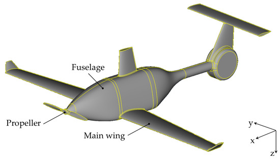
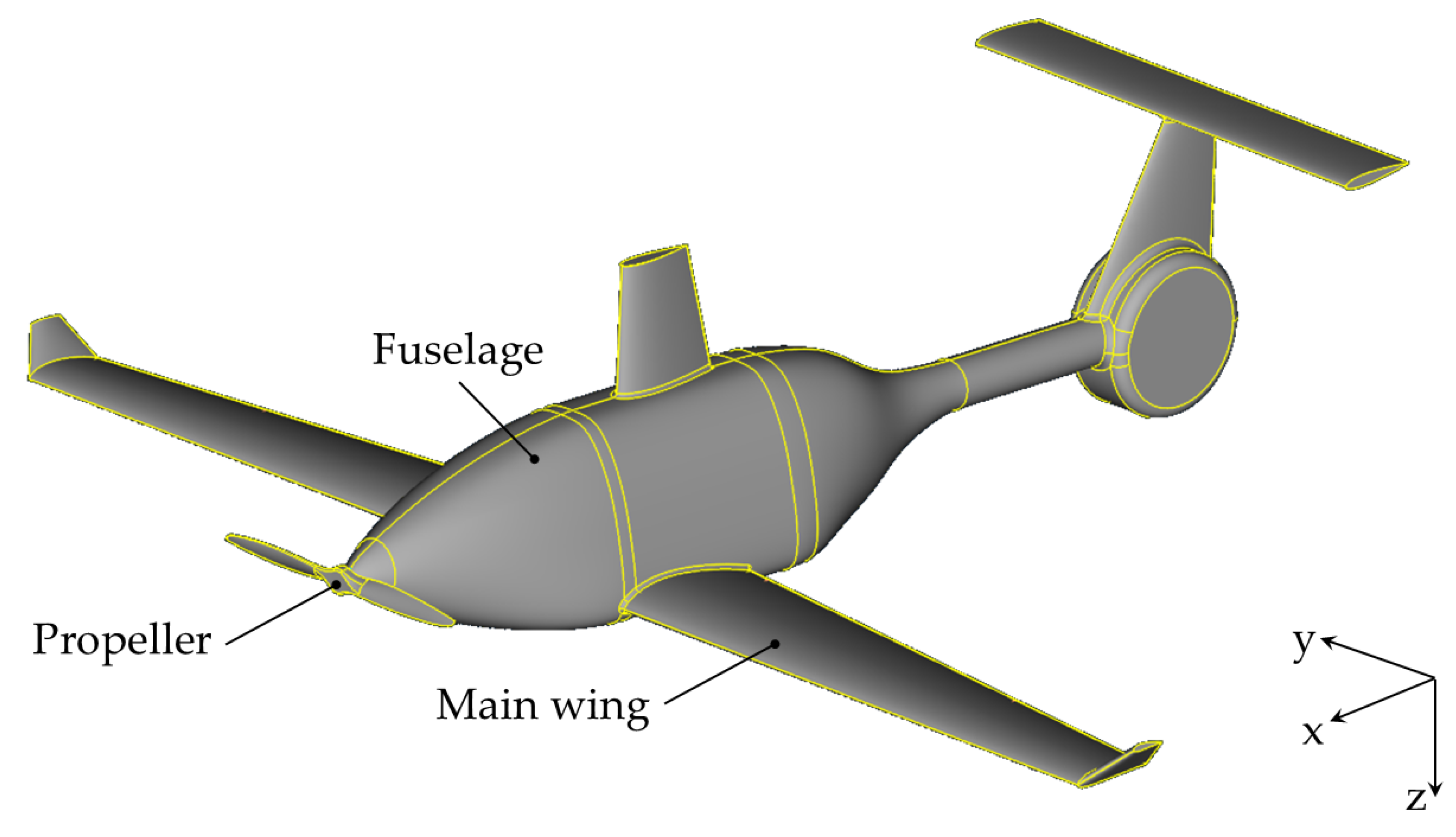
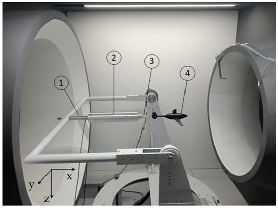
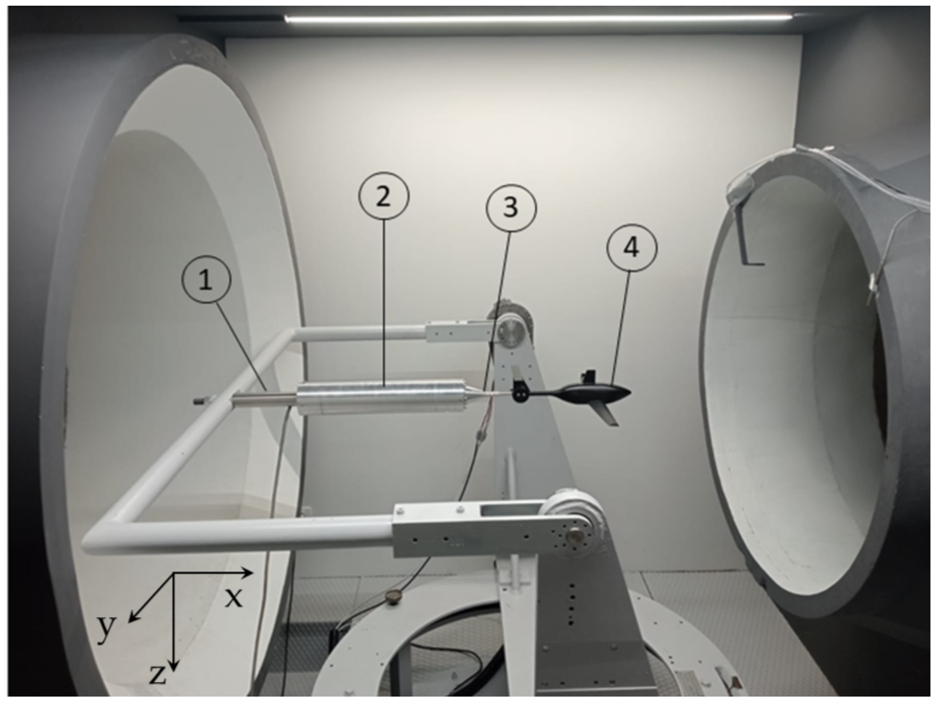
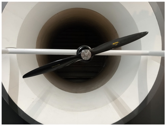
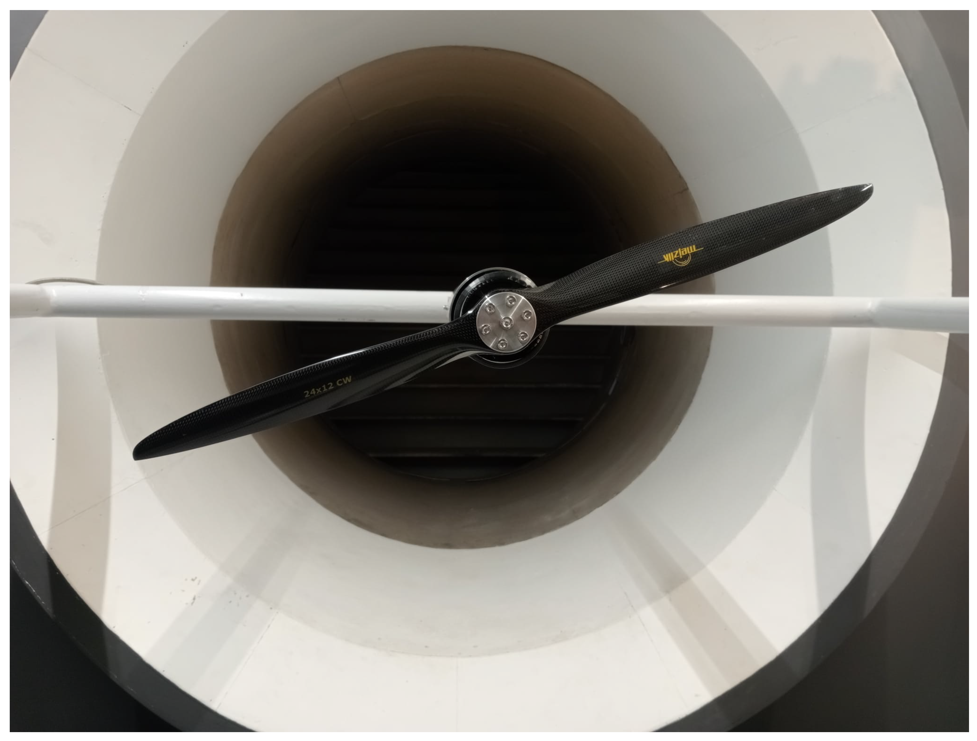
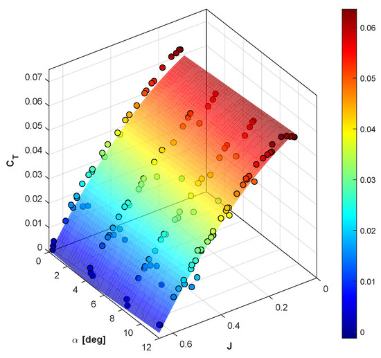
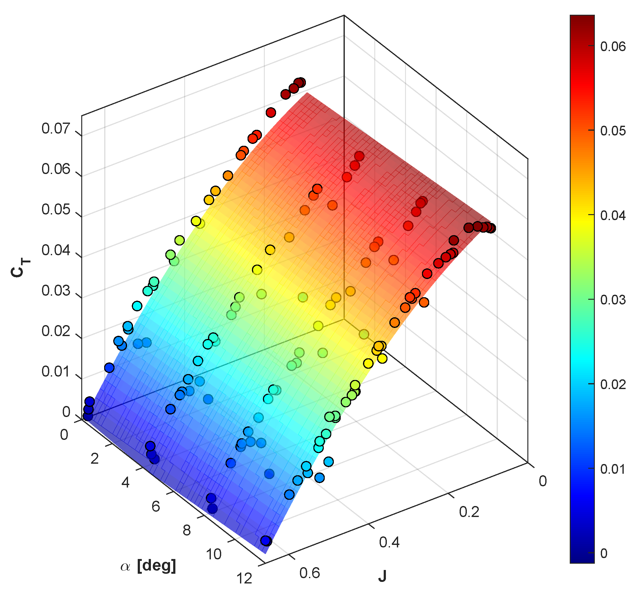
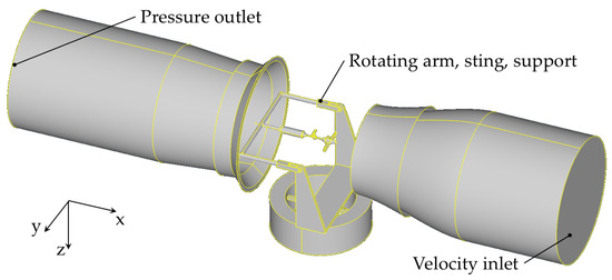
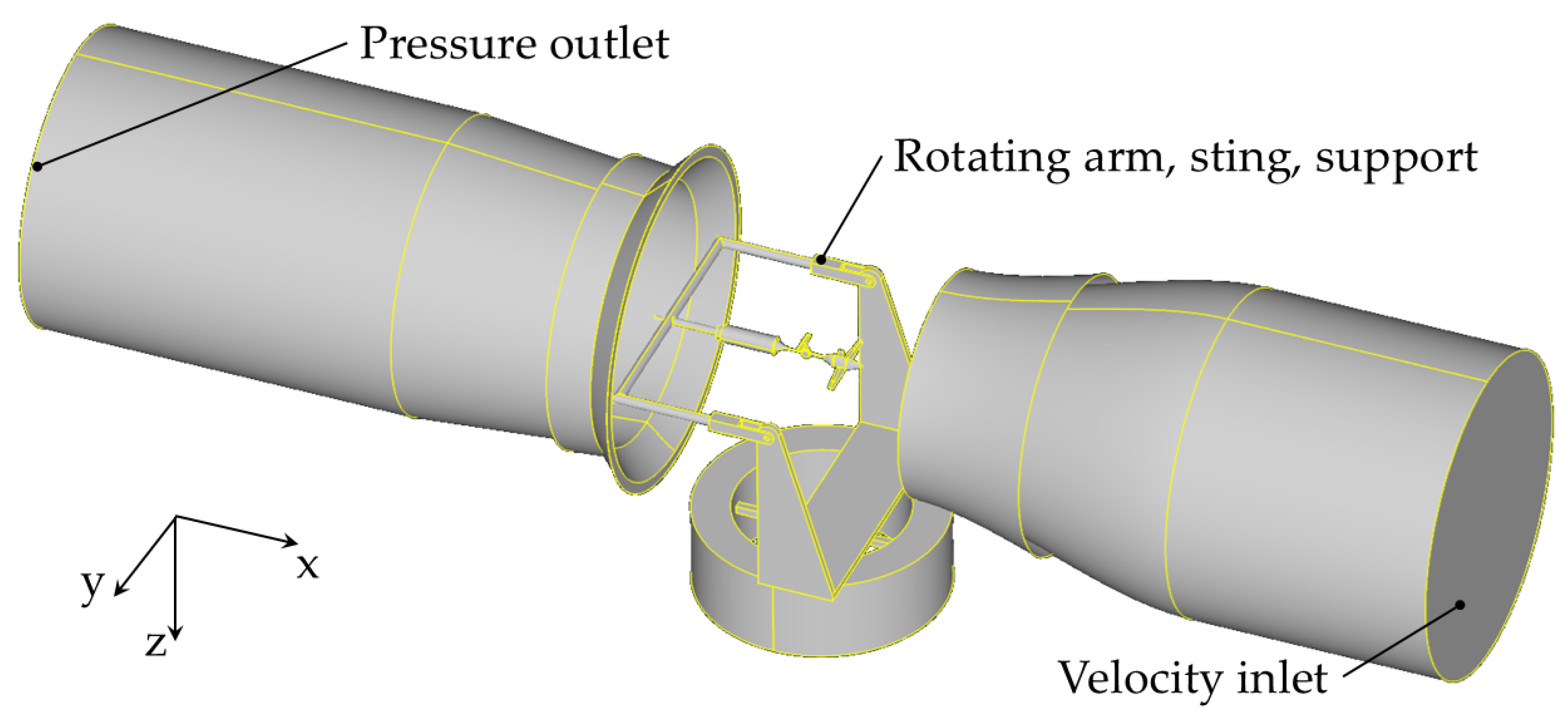
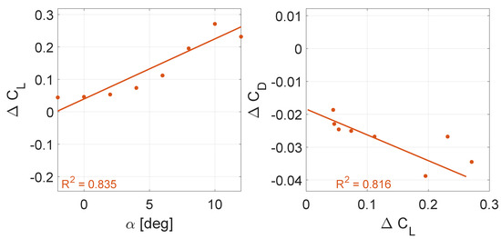
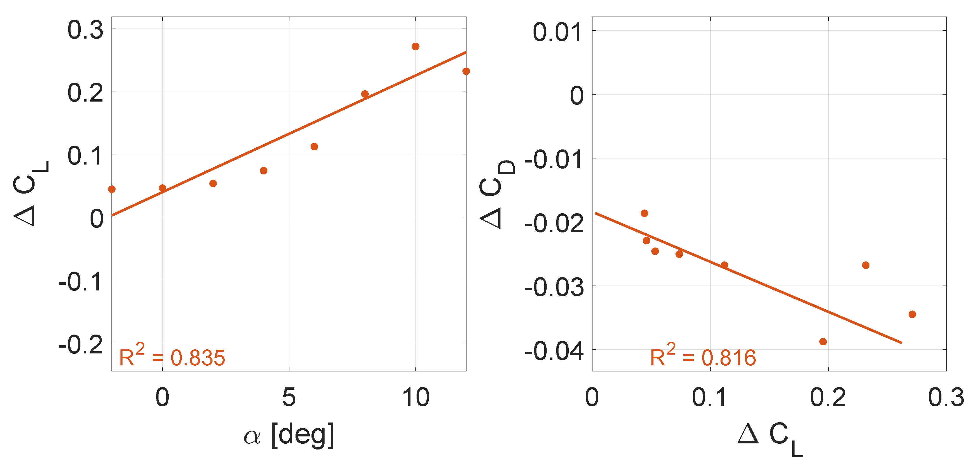
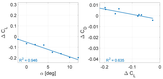
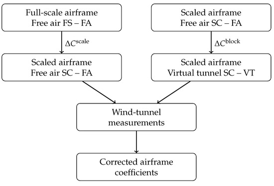
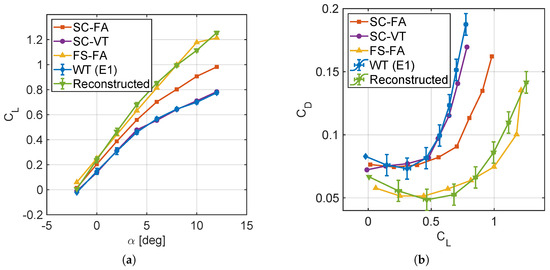
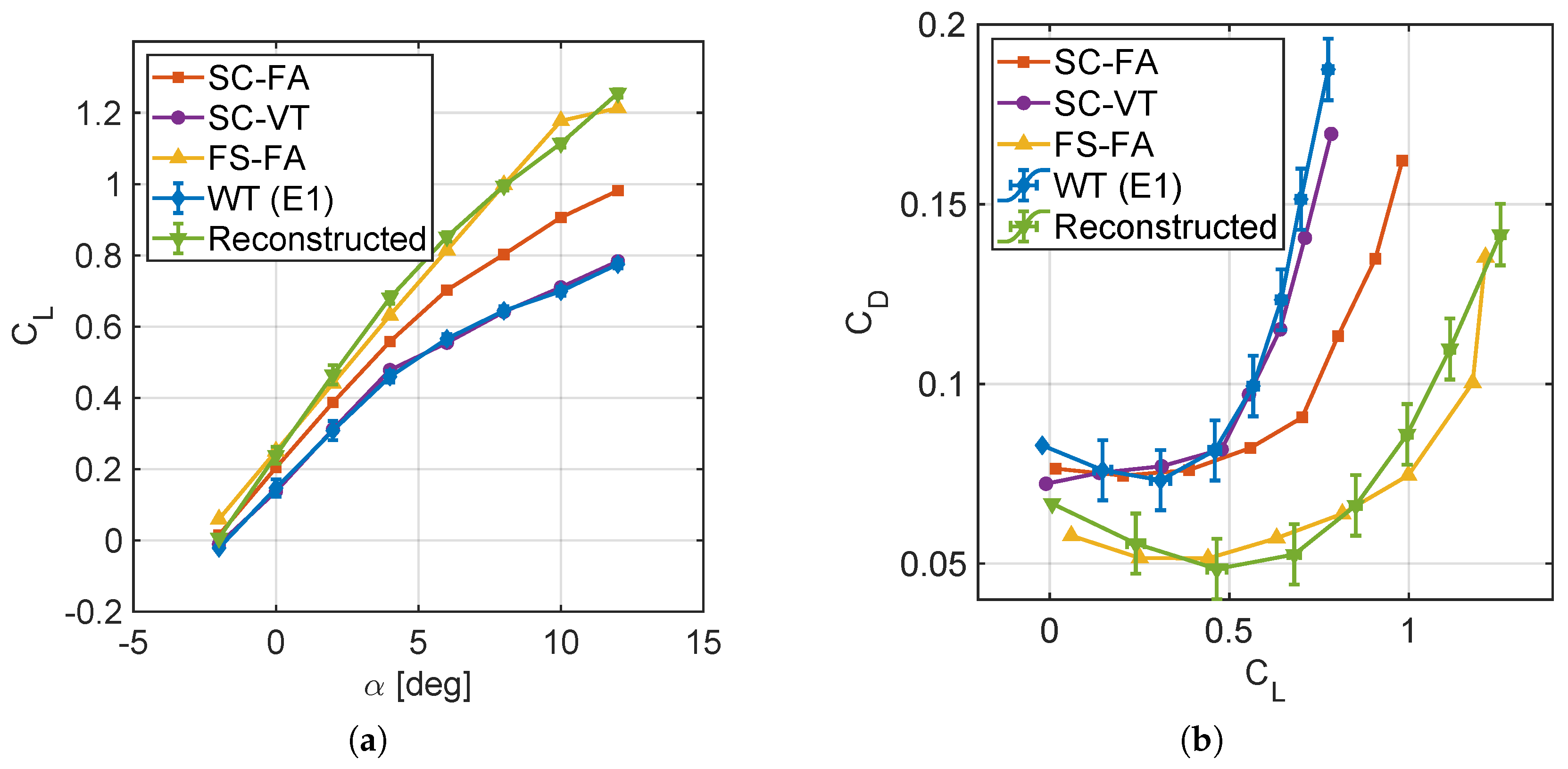
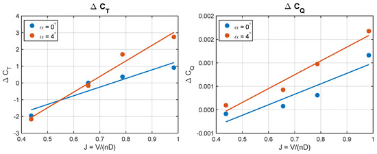
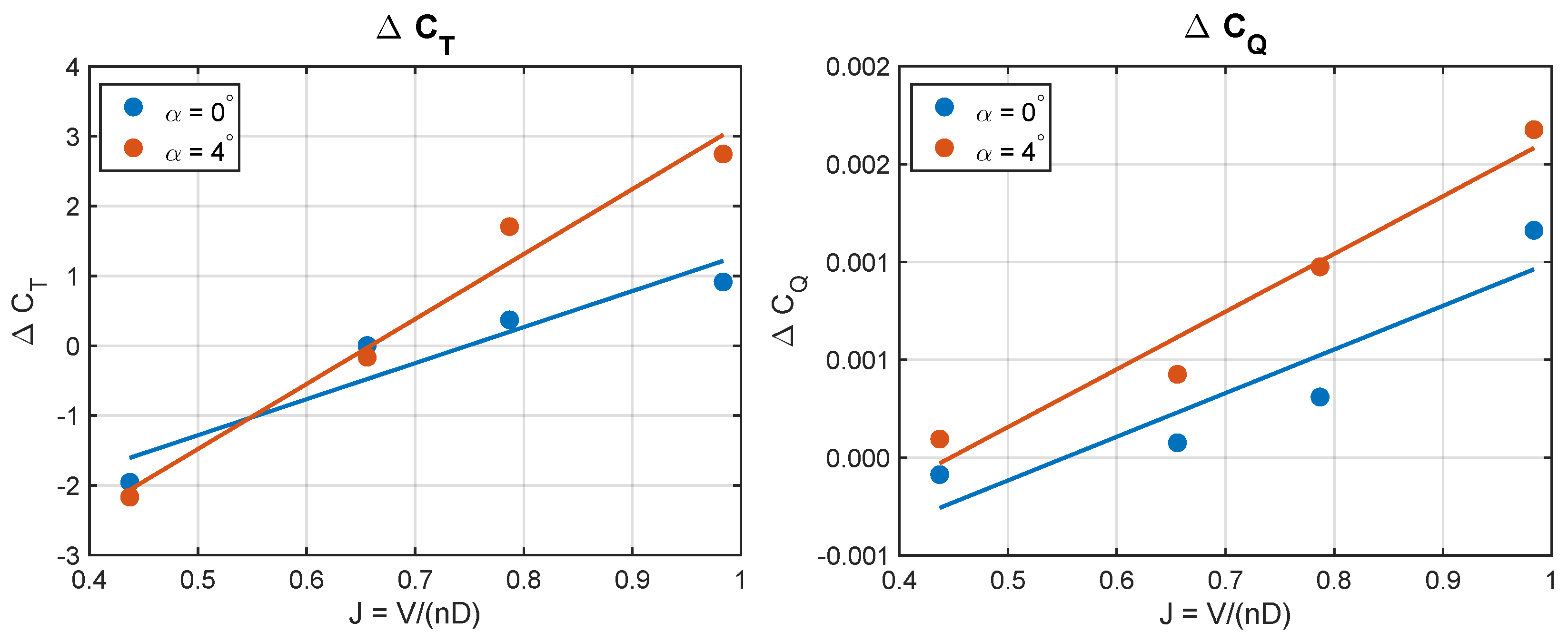
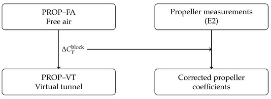
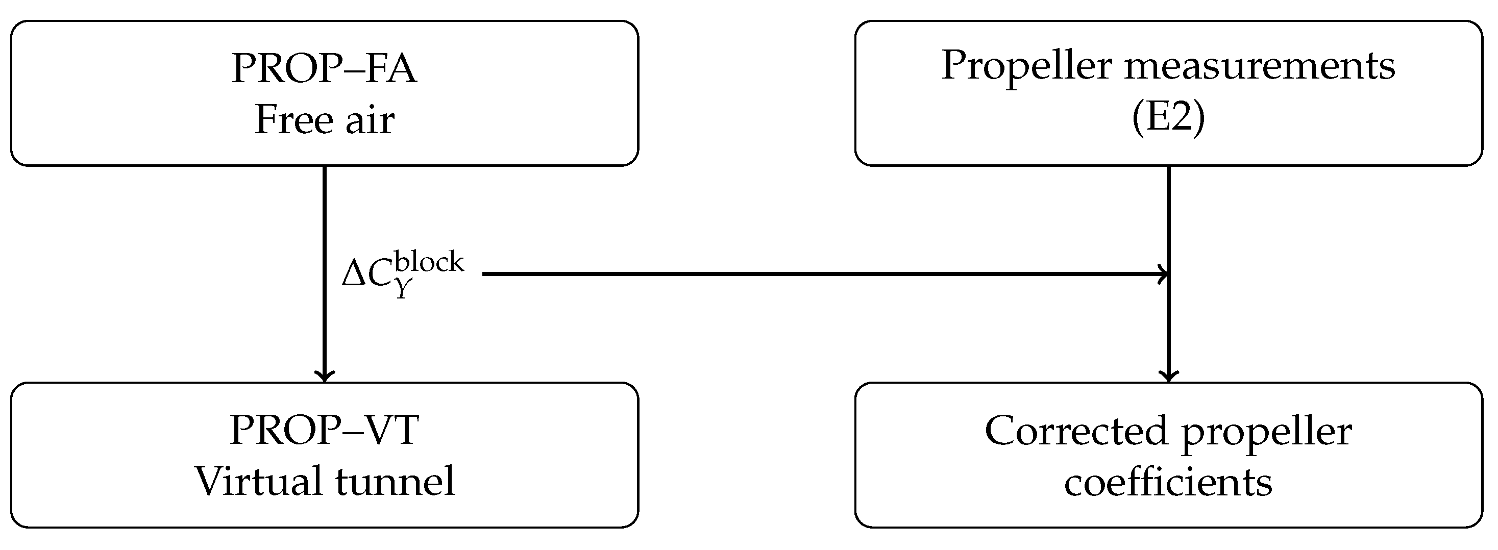
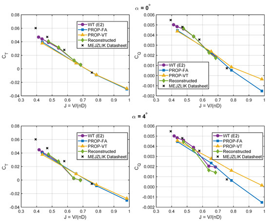
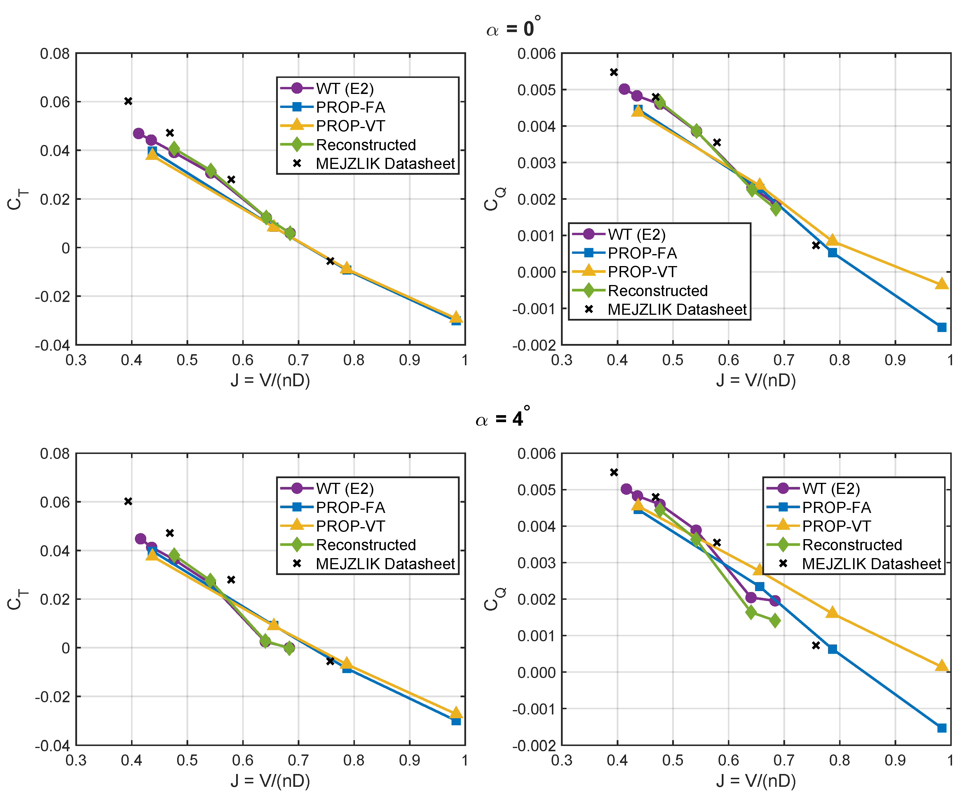
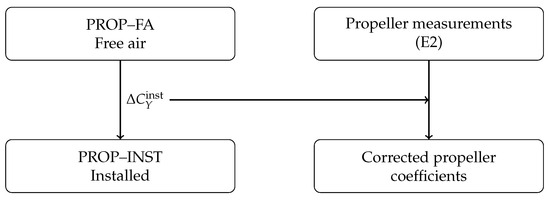
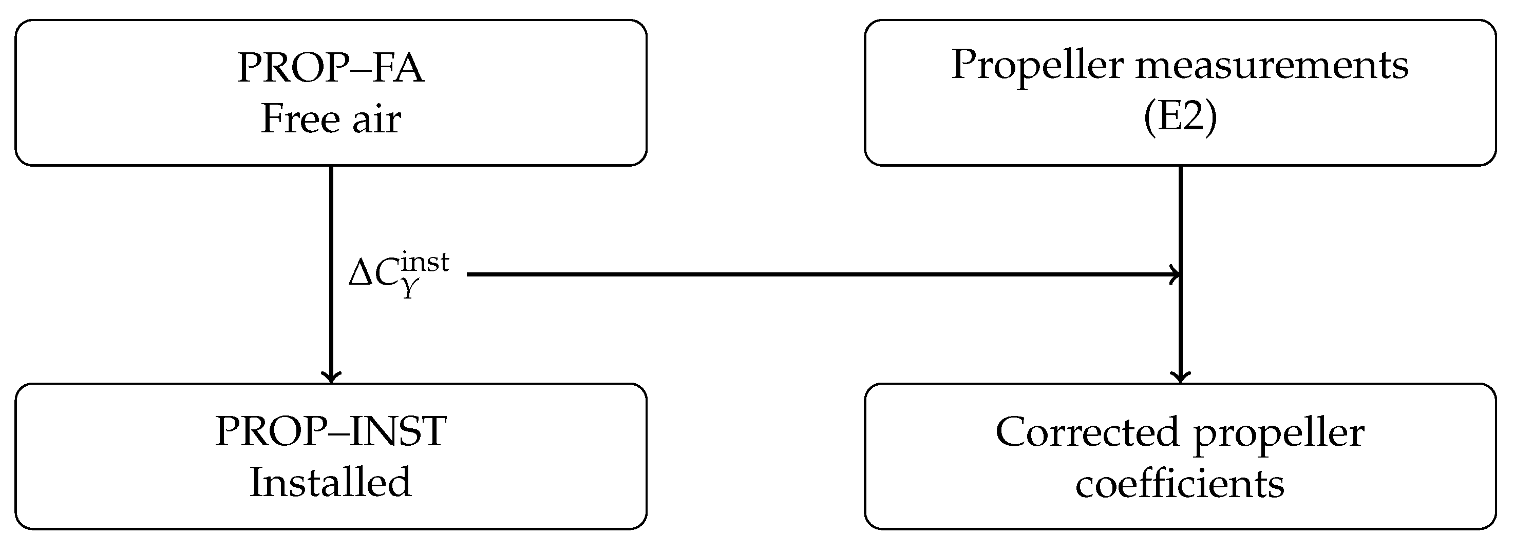
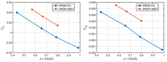
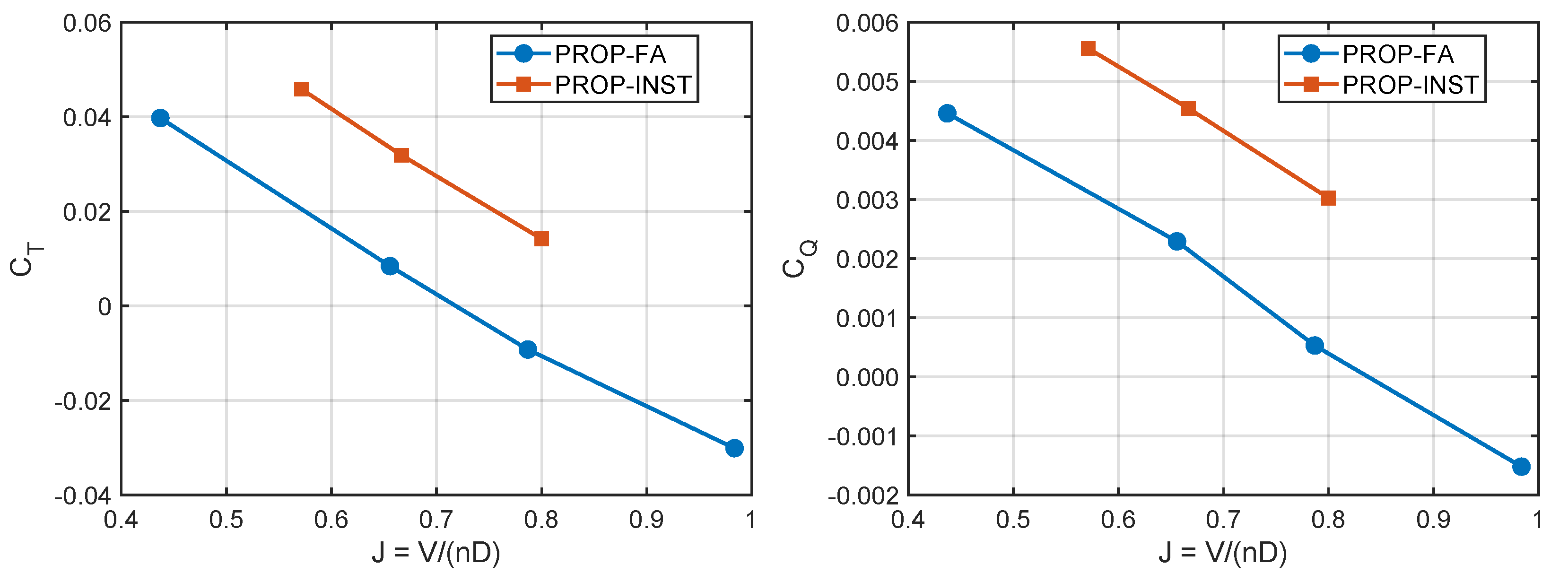
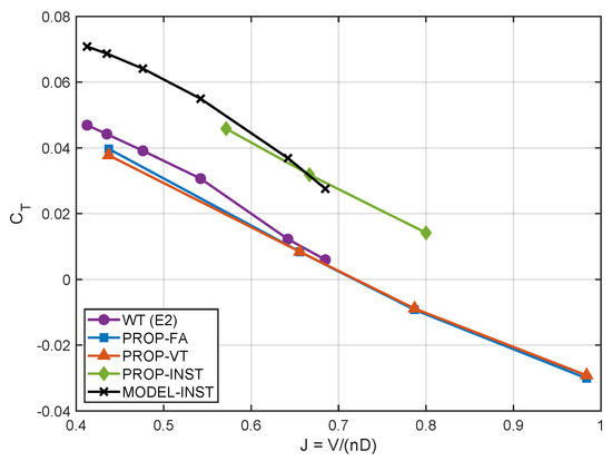
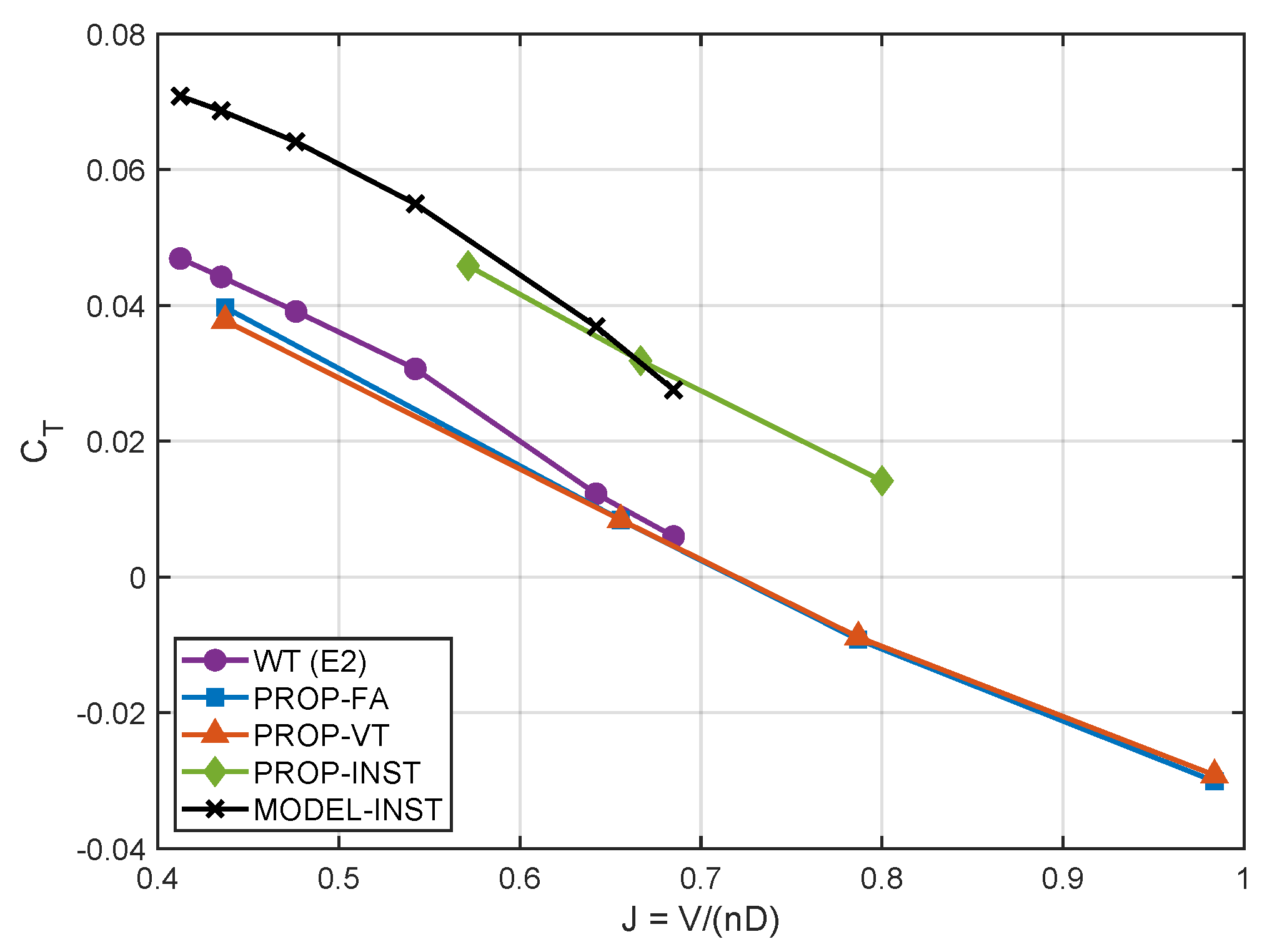
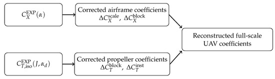
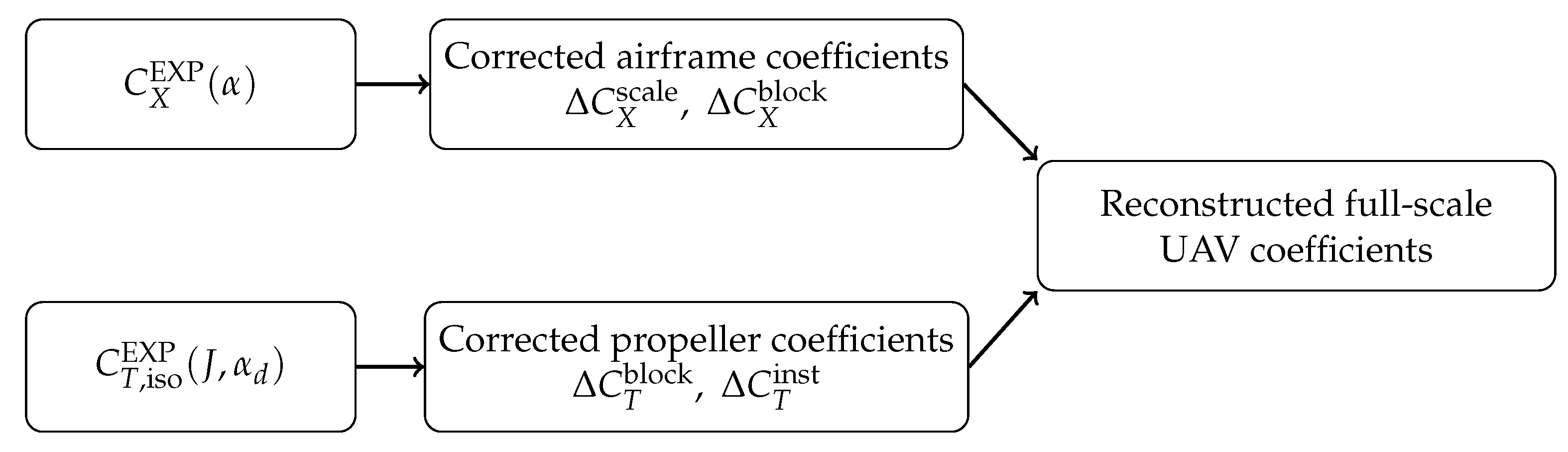

Disclaimer/Publisher’s Note: The statements, opinions and data contained in all publications are solely those of the individual author(s) and contributor(s) and not of MDPI and/or the editor(s). MDPI and/or the editor(s) disclaim responsibility for any injury to people or property resulting from any ideas, methods, instructions or products referred to in the content. |
© 2026 by the authors. Licensee MDPI, Basel, Switzerland. This article is an open access article distributed under the terms and conditions of the Creative Commons Attribution (CC BY) license.